




1. Introduction
A rapidly increasing number of applications involve flows in confined microscale channels, that is, in the field of microfluidics (Stone, Stroock & Adjari Reference Stone, Stroock and Adjari2004). Among other phenomena, attention is paid to hydrodynamic dispersion (Ng Reference Ng2011) and field-flow fractionation (Giddings, Yang & Myers Reference Giddings, Yang and Myers1976, Reference Giddings, Yang and Myers1977).
At these small scales, viscous dissipation becomes preponderant, requiring a high-pressure head for liquids to flow in microchannels. This is also a key issue for transporting suspensions of particles in such confined geometries. This is the domain of microrheology. In this field, non-optical microrheology is developing rapidly in search of technical solutions (Vleminckx & Clasen Reference Vleminckx and Clasen2014). The so-called microcapillary rheometer is related to the problem considered here.
The effective viscosity of a confined flowing suspension is the relevant quantity to consider for this energy budget problem (see, for example, the experiments of Peyla & Verdier (Reference Peyla and Verdier2011)). A suspension effective viscosity depends on the volume fraction magnitude and distribution and also on the ambient flow field when the suspension flows in a confined geometry. Assuming a dilute suspension (i.e. a small particle volume fraction), Navardi & Bhattacharya (Reference Navardi and Bhattacharya2010) derived the effective viscosity of a suspension of spherical particles in a cylindrical no-slip conduit. Then, Feuillebois et al. (Reference Feuillebois, Ekiel-Jeżewska, Wajnryb, Sellier and Bławzdziewicz2015) and Feuillebois et al. (Reference Feuillebois, Ekiel-Jeżewska, Wajnryb, Sellier and Bławzdziewicz2016) derived the effective viscosity of a dilute suspension bounded by parallel no-slip walls for a Couette flow and a Poiseuille flow, respectively. Their results were obtained in terms of singularities on individual particles, i.e. the classical stresslet for Couette flow, to which a quadrupole is added for Poiseuille flow. The particles considered had various shapes. As for the particle distribution between walls, they considered a high-frequency ambient flow field, in the sense that all particles occupy all possible positions and orientations with equal probability.
The energy cost for transporting suspensions in microchannels may be reduced by using slipping walls. This issue motivates the present article. We are concerned here with the Poiseuille flow for a dilute monodisperse suspension of solid, no-slip, spherical particles between two solid, impermeable, slip, parallel plane walls. On each wall the impermeability condition reads  ${\boldsymbol {u}}\boldsymbol {\cdot } {\boldsymbol {n}}=0$, where ${\boldsymbol {u}}$ is the fluid velocity and ${\boldsymbol {n}}$ is the unit vector normal to the wall and pointing into the liquid. The usual Navier (Reference Navier1823) slip boundary condition is applied on each wall where it reads
 \begin{equation} {\boldsymbol{u}}=\lambda \frac{\partial {\boldsymbol{u}}}{\partial n}, \end{equation}
where  $\lambda \geq 0$ is the wall slip length, assumed to be uniform and identical for both walls, and $n$ is the normal coordinate along ${\boldsymbol {n}}$. Using a simple classical interpretation of (1.1) boundary condition on an impermeable wall, it is equivalent to the no-slip boundary condition on a fictitious no-slip wall that would be shifted away from the liquid by a distance $\lambda$. In the light of this simple model one could think of directly applying the results of Feuillebois et al. (Reference Feuillebois, Ekiel-Jeżewska, Wajnryb, Sellier and Bławzdziewicz2016) for spheres and to a wider channel (with width increased by $2\lambda$) in order to predict the suspension effective viscosity in the presence of slip. It will be seen later in the article that this naive concept is not sufficient.
In Feuillebois et al. (Reference Feuillebois, Ekiel-Jeżewska, Wajnryb, Sellier and Bławzdziewicz2015, Reference Feuillebois, Ekiel-Jeżewska, Wajnryb, Sellier and Bławzdziewicz2016) the hydrodynamic interactions with both no-slip walls were taken into account exactly using the proper Green velocity tensor obtained by Liron & Mochon (Reference Liron and Mochon1976) and revisited for numerical implementation by Jones (Reference Jones2004). Unfortunately, no such Green tensor exists, to our knowledge, for slip walls. To circumvent this problem, following Pasol et al. (Reference Pasol, Martin, Ekiel-Jeżewska, Wajnryb, Bawzdziewicz and Feuillebois2011), each slip wall contribution is here taken into account separately. In practice, two different approaches are used: the nearest-wall model (denoted as nw) and the wall-superposition model (denoted as ws). These two models, which will be made more precise later on when necessary, only require the solutions for flows around a sphere near a slip plane wall. These solutions were obtained using bipolar coordinates which have a long history (see e.g. Pasol, Sellier & Feuillebois (Reference Pasol, Sellier, Feuillebois, Feuillebois and Sellier2009) and references therein). Here we will use the results of Loussaief, Pasol & Feuillebois (Reference Loussaief, Pasol and Feuillebois2015) and Ghalia, Feuillebois & Sellier (Reference Ghalia, Feuillebois and Sellier2016) for a sphere suspended in linear and quadratic ambient shear flows, respectively.
This article is organized as follows. Formal expressions of the effective and associated intrinsic viscosities of a dilute suspension of solid spheres in Poiseuille flow between two parallel solid slip impermeable walls are first defined and derived in § 2. The intrinsic viscosity is expressed in terms of one Cartesian component of the stresslet tensor and one component of the quadrupole tensor (see Feuillebois et al. Reference Feuillebois, Ekiel-Jeżewska, Wajnryb, Sellier and Bławzdziewicz2016). These two key quantities are obtained in § 3 from the nw and ws approximations. Both approximations reduce the problem to the hydrodynamic interaction of a single sphere with one plane slip wall. This latter problem is accurately solved using bipolar coordinates. The calculation of the quadrupole term is presented in § 3.3 and benchmarked against a boundary element method in § 3.4. The results for the intrinsic viscosity are presented in § 4 for different values of the gap between walls and of the wall slip length  $\lambda \leq a$, where $a$ denotes the sphere radius (this upper bound on $\lambda$ being satisfied for most encountered applications). A handy interpolation formula is derived therefrom in § 4.4. Finally, a discussion and conclusion are presented in § 5.
2. Formal expression of the effective viscosity of a dilute suspension
This section starts with the expression of the ambient Poiseuille flow between parallel slip walls (§ 2.1). The definition of the effective viscosity of the suspension of no-slip particles for this geometry and flow field is given in § 2.2. The approach to the derivation of a formal expression of the effective viscosity goes along the lines used for the case of a Poiseuille flow between parallel no-slip walls by Feuillebois et al. (Reference Feuillebois, Ekiel-Jeżewska, Wajnryb, Sellier and Bławzdziewicz2016) (that article is denoted below as (I)) and is presented in § 2.3. It is shown that the approach using the Lorentz reciprocal theorem for no-slip walls carries over to the case of slip walls. Only the main intermediate formulae which differ from those of that earlier article are displayed here. The final formula for the effective viscosity is specialized for the case of a dilute monodisperse suspension of spheres in § 2.4.
2.1. The ambient Poiseuille flow
Consider (figure 1) a channel between two parallel walls  $W_1,W_2$ separated by a distance $H$. We use a Cartesian coordinate system $(x,y,z)$ with axes $(x,y)$ along the walls and $z$ perpendicular to the walls, such that the walls $W_1$ and $W_2$ are in the planes $z=0$ and $z=H$, respectively.
Sketch of a single sphere with centre  $O'$ and radius $a$ freely suspended in a Poiseuille flow between two parallel solid slip walls $W_1$ and $W_2.$
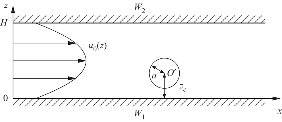
The Poiseuille fluid flow is driven by an imposed constant pressure gradient  ${\rm \Delta} p_0/L$ along the $x$ direction, where $L$ is a length along $x$ that is large compared with $H$ (but small compared with a characteristic channel dimension in the $y$ direction) and ${\rm \Delta} p_0=p_0(L/2)-p_0(-L/2)$ is the negative pressure drop between the far away upstream and downstream sections.
In this article, we consider slip walls with equal slip lengths  $\lambda$ on both walls. The expression for the Poiseuille flow velocity along $x$ is easily found to be (Feuillebois, Bazant & Vinogradova Reference Feuillebois, Bazant and Vinogradova2009; Ng Reference Ng2011)
 \begin{equation} u_0(z)=k_1(z+\lambda)+k_2 z^{2} \end{equation}
and the corresponding pressure may be written as
 \begin{equation} p_0(x)= 2\mu_0 k_2 x \end{equation}
with the constant coefficients
 \begin{equation} k_1=-\frac{H}{2\mu_0} \frac{{\rm \Delta} p_0}{L} ,\quad k_2=-\frac{k_1}{H}, \end{equation}
which are independent of the slip length. The local shear rate at a position  $z$ between the planes
 \begin{equation} \dot{\gamma}(z)=k_1 + 2 k_2 z \end{equation}
is thus also independent of  $\lambda$.
The volume flow rate  $\bar {u}_0 H$ (per unit channel length in the transverse direction $y$) is expressed in terms of the fluid velocity averaged across the channel width:
 \begin{equation} \bar{u}_0 = \frac 1H \int_{z=0}^{H} u_0(z) \, \textrm{d}z. \end{equation}
By inserting (2.1) and (2.3a,b) into (2.5) we obtain the expression
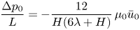 \begin{equation} \frac{{\rm \Delta} p_0}{L} = -\frac{12}{H(6\lambda+H)} \, \mu_0 \bar{u}_0 \end{equation}
for the pressure drop per unit length of the channel.
2.2. Definition of the effective viscosity of the suspension
Consider now that the channel contains a dilute suspension of solid no-slip particles of typical length scale  $a$. The suspension is entrained along $x$ by a constant pressure gradient that is, by comparison with the pure fluid, affected by the presence of particles.
Similarly to (2.9) in (I), the effective viscosity of the suspension is defined from the linear relationship between the volume flow rate  $\bar {u}_0H$ and the average pressure gradient that is necessary to drive the flow field on a distance $L$ such that $L/H\to \infty$ with $H/a$ fixed. Like in (I), there are no effects of the far away container walls in the $y$ direction at distances large compared with $L$. Then, taking an average (denoted by $\left\langle \cdot \right\rangle$) over all possible positions and orientations of the particles
 \begin{equation} \left\langle \lim_{L\to\infty}\frac{{\rm \Delta} P}{L}\right\rangle = -\frac{12}{H(6 \lambda+H)} \, \mu_{\textit{eff}} \,\bar{u}_0 \end{equation}
defines the effective viscosity  $\mu _{\textit{eff}}$, the search for which is the goal of this article.
2.3. Application of Lorentz reciprocal theorem
The flow field perturbed by the presence of particle  $i$ is sought as the sum of the unperturbed flow (indicated by subscript $0$) and a perturbation (indicated by a prime). Accordingly, the perturbed flow velocity, stress tensor and pressure are written as
 \begin{gather} {\boldsymbol{u}} = {\boldsymbol{u}}_0 + {\boldsymbol{u}}',\quad \boldsymbol{\sigma} = \boldsymbol{\sigma}_0 + \boldsymbol{\sigma}',\quad p = p_0 + p' . \end{gather}
It will not be necessary to calculate the perturbed flow field in full detail. Indeed, the method of solution uses the Lorentz reciprocal theorem, as in (I) (3.1a,b):
 \begin{equation} \int_{(S_i\cup S_L\cup S_{\textit{width}}\cup W)} {\boldsymbol{u}}_0\boldsymbol{\cdot} \boldsymbol{\sigma}'\boldsymbol{\cdot} {\boldsymbol{n}} \,\textrm{{d}}S = \int_{(S_i\cup S_L\cup S_{\textit{width}}\cup W)} {\boldsymbol{u}}'\boldsymbol{\cdot} \boldsymbol{\sigma}_0\boldsymbol{\cdot} {\boldsymbol{n}} \,\textrm{{d}}S , \end{equation}
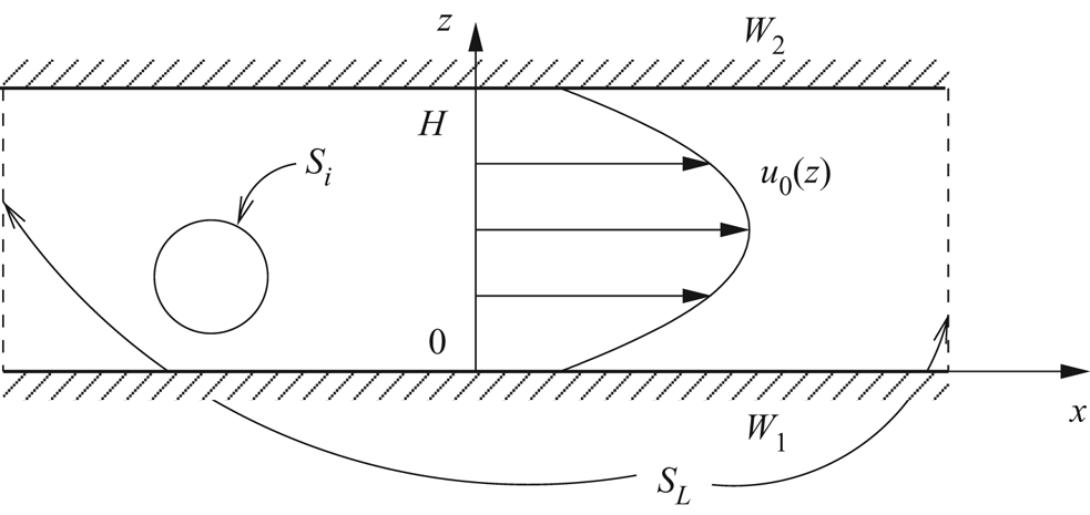
where (see the control volume in figure 2)  $S_i$ is the surface of a given particle labelled $i$,
$i$,  $S_L$ is the set of surfaces tending to infinity upstream and downstream, $S_{width}$ is the set of surfaces tending to infinity in the $y$ direction (not shown in figure 2) and $W=W_1\cup W_2$.
Control volume for the application of the Lorentz reciprocal theorem.
The derivation is as in (I):
(i) Integrals over $S_i$ take into account the no-slip boundary condition on the particle and their calculation is the same as in (I). They involve the force, torque, stresslet and quadrupole components $S_{i,xz}$ and $Q_{i,xzz}$. These quantities $S_{i,xz}$ and $Q_{i,xzz}$ are, respectively, the $(x,z)$ component of the second-order stresslet tensor ${\boldsymbol {S}}_i$ and the $(x,z,z)$ component of the third-order quadrupole tensor ${\boldsymbol {Q}}_i$ on particle $i$. These tensors are defined as
(2.10)\begin{gather} {\boldsymbol{S}}_i = \int_{S_i} \left[\tfrac{1}{2}({\boldsymbol{r}}_i\, {\boldsymbol{f}}+ {\boldsymbol{f}} {\boldsymbol{r}}_i)-\tfrac{1}{3} ({\boldsymbol{r}}_i\boldsymbol{\cdot} {\boldsymbol{f}}) {\boldsymbol{I}} \right]\textrm{d}S, \end{gather}(2.11)Here,\begin{gather} {\boldsymbol{Q}}_i = \int_{S_i} {\boldsymbol{f}} \; {\boldsymbol{r}}_i {\boldsymbol{r}}_i \,\textrm{{d}}S. \end{gather}${\boldsymbol {f}}$ is the stress of the perturbed flow field on particle $i$ and ${\boldsymbol {r}}_i$ is a vector pointing from the centre of particle $i$ to a point on its surface $S_i$.
$S_i$ take into account the no-slip boundary condition on the particle and their calculation is the same as in (I). They involve the force, torque, stresslet and quadrupole components $S_{i,xz}$ and $Q_{i,xzz}$. These quantities $S_{i,xz}$ and $Q_{i,xzz}$ are, respectively, the $(x,z)$ component of the second-order stresslet tensor ${\boldsymbol {S}}_i$ and the $(x,z,z)$ component of the third-order quadrupole tensor ${\boldsymbol {Q}}_i$ on particle $i$. These tensors are defined as
(2.10)\begin{gather} {\boldsymbol{S}}_i = \int_{S_i} \left[\tfrac{1}{2}({\boldsymbol{r}}_i\, {\boldsymbol{f}}+ {\boldsymbol{f}} {\boldsymbol{r}}_i)-\tfrac{1}{3} ({\boldsymbol{r}}_i\boldsymbol{\cdot} {\boldsymbol{f}}) {\boldsymbol{I}} \right]\textrm{d}S, \end{gather}(2.11)Here,\begin{gather} {\boldsymbol{Q}}_i = \int_{S_i} {\boldsymbol{f}} \; {\boldsymbol{r}}_i {\boldsymbol{r}}_i \,\textrm{{d}}S. \end{gather}${\boldsymbol {f}}$ is the stress of the perturbed flow field on particle $i$ and ${\boldsymbol {r}}_i$ is a vector pointing from the centre of particle $i$ to a point on its surface $S_i$.(ii) Integrals on
$S_L$ give the supplementary force difference ${\rm \Delta}\,f'$ (between the upstream and downstream far away sections) that is necessary to drive the particle $i$.(iii) Integrals on
$S_{width}$ (in the $y$ direction) vanish.


The main difference from (I) is in the calculation of the integrals on the slip walls  $W_1$ and $W_2$ in (2.9), which cancel out, as we will see now.
For this purpose, we rewrite the integrands in terms of their components in the  $(x,y,z)$ directions. The unperturbed flow velocity ${\boldsymbol {u}}_0$ on the wall is in the $x$ direction and so is the stress of the unperturbed flow field on the wall:
 \begin{equation} {\boldsymbol{u}}_0 = u_0 \, {\boldsymbol{e}}_x,\quad \boldsymbol{\sigma}_0\boldsymbol{\cdot} {\boldsymbol{n}} = f_0 \, {\boldsymbol{e}}_x, \end{equation}
where  $u_0$ and $f_0$ are, respectively, the velocity (2.1) and stress components in the $x$ direction. The perturbed flow velocity ${\boldsymbol {u}}'$ on the wall has components in the $x$ and $y$ directions since the wall is impermeable; now, the stress of the perturbed flow may have all its components $(\,f'_x,f'_y,f'_z)$:
 \begin{equation} {\boldsymbol{u}}'=u'_x {\boldsymbol{e}}_x+u'_y {\boldsymbol{e}}_y,\quad \boldsymbol{\sigma}'\boldsymbol{\cdot} {\boldsymbol{n}} = f'_x {\boldsymbol{e}}_x+f'_y {\boldsymbol{e}}_y+f'_z {\boldsymbol{e}}_z. \end{equation}
The integral on  $W_1$ on the left-hand side of (2.9) is then written
 \begin{equation} \int_{W_1} u_0\, f'_x \,\textrm{{d}}S \end{equation}
and the integral on  $W_1$ on the right-hand side of (2.9) is written
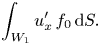 \begin{equation} \int_{W_1} u'_x\, f_0 \,\textrm{{d}}S. \end{equation}
The slip conditions on the wall  $W_1$ are written for the unperturbed and perturbed flow fields in the $x$ direction as
 \begin{equation} u_0 = \frac{\lambda}{\mu} f_0,\quad u'_x=\frac{\lambda}{\mu}\, f'_x, \end{equation}
where  $\lambda$ is the slip length on $W_1$. Substituting these conditions into (2.14) and (2.15) shows that these integrals are equal. Thus they compensate in (2.9). Likewise, it can be shown that the integrals on $W_2$, where the same slip length $\lambda$ applies, compensate in (2.9). Therefore, even though the integrals on the walls do not vanish as in the no-slip case in (I), the same formal approach may be carried out here for the slip walls.
Finally, from (2.9) the supplementary necessary force difference  ${\rm \Delta}\,f'$ between the upstream and downstream far away sections that is necessary to drive the particle $i$ is (as in (3.20a,b) in (I))
 \begin{equation} u_0(z_i)F_{i,x}+ \dot{\gamma}(z_i)C_{i,y}+ \dot{\gamma}(z_i) S_{i,xz} + k_2 Q_{i,xzz} + {\rm \Delta} f' \,\bar{u}_0 =0 . \end{equation}
Here,  $F_{i,x}$ and $C_{i,y}$ are, respectively, the force in direction $x$ and the torque in direction $y$ on particle $i$.
$i$.
As in (I), (2.17) is generalized to a suspension of  $N$ particles ( $i=1\ldots N$) contained in a control volume $V$. We then obtain the supplementary force difference ${\rm \Delta} F' = \sum _{i=1}^{N} f'$ that is necessary to drive the suspension. Dividing ${\rm \Delta} F'$ by the volume $V$ containing the $N$ particles and taking the thermodynamic limit for $L\to \infty$ (with $N\to \infty$ and $n=N/V$ kept finite) yields the following result (like (3.22) in (I)):
 \begin{equation} \lim_{ L\to\infty} \frac{{\rm \Delta} P'}{ L} = -\frac{1}{\bar{u}_0} \lim_{ L\to\infty} \frac{1}{V} \sum_{i=1}^{N} \left[ u_0(z_i)F_{i,x}+ \dot{\gamma}(z_i)C_{i,y}+ \dot{\gamma}(z_i) S_{i,xz} + k_2 Q_{i,xzz} \right]. \end{equation}
From (2.7), the average  $\left\langle {.} \right\rangle$ over all possible positions and orientations of the particles of this quantity provides the effective viscosity $\mu _{\textit{eff}}$. For force-free and torque-free particles, $F_{i,x}=C_{i,y}=0$, the result is
 \begin{equation} \mu_{\textit{eff}} = \mu_0 + \frac{H(H+6\lambda)}{12\bar{u}_0^{2}} \left\langle \lim_{ L\to\infty} \frac{1}{V} \sum_{i=1}^{N} \left[ \dot{\gamma}(z_i) S_{i,xz} + k_2 Q_{i,xzz} \right] \right\rangle . \end{equation}
This formula is quite general, in the sense that it applies to any particle shape in any polydisperse dilute suspension.
2.4. Dilute monodisperse suspension of spheres
The considered suspension is monodisperse. It is also assumed to be dilute in the sense that its volume fraction  $\phi =Nv/V$ is small compared with unity, where $v$ is the volume of one particle. It is standard for this suspension to introduce the intrinsic viscosity defined as $[\mu ]=(\mu_{\textit{eff}}-\mu _0)/(\mu _0 \phi )$.
In a monodisperse suspension all particle contributions are statistically equivalent, so that (2.19) yields the intrinsic viscosity:
 \begin{equation} [\mu] = \frac{H(H+6\lambda)}{12 \bar{u}_0^{2} v \mu_0} \left\langle \dot{\gamma}(z) S_{xz} + k_2 Q_{xzz} \right\rangle . \end{equation}
Here the index  $i$ has been dropped for a test particle that is identical to the other ones. The centre of this particle is denoted $z_c$. Equation (2.20) replaces (4.5) in (I); $H$ there is replaced here by $H(H+6\lambda )$ in the numerator of the prefactor; moreover, the stresslet $S_{xz}$ and quadrupole $Q_{xzz}$ components both depend on the slip length $\lambda$ on the walls. Recalling (2.3a,b) and writing all constants in terms of $k_1$, the final result is
 \begin{equation} [\mu] = \frac{3}{\mu_0 v k_1(1+6\lambda/H)} \left\langle \left( 1 -2 \frac{z_c}{H} \right) S_{xz} -\frac{Q_{xzz}}{H} \right\rangle . \end{equation}
This equation replaces the result (4.6) for no-slip walls in (I).
Consider now spherical particles of radius  $a$ and volume $v=\frac 43 {\rm \pi} a^{3}$. We define the dimensionless channel width, particle centre coordinate and slip length as
 \begin{equation} \tilde{H}=\frac{H}{a} ,\quad \tilde{z}_{c}=\frac{z_c}{a},\quad \tilde{\lambda}=\frac{\lambda}{a} \end{equation}
and the dimensionless stresslet and quadrupole as
 \begin{gather} \tilde{S}_{xz} = \frac{S_{xz}}{\mu_0 a^{3} k_1},\quad \tilde{Q}_{xzz} = \frac{Q_{xzz}}{\mu_0 a^{4} k_1}. \end{gather}
Equation (2.21) can then be recast in dimensionless form as
 \begin{equation} [\mu] = \frac{9}{4{\rm \pi}(1+6 \tilde{\lambda}/ \tilde{H})} \left\langle \left( 1 -2 \frac{ \tilde{z}_{c}}{ \tilde{H}} \right) \tilde{S}_{xz} -\frac{1}{ \tilde{H}} \tilde{Q}_{xzz} \right\rangle . \end{equation}
 As in (I) and in Navardi & Bhattacharya (Reference Navardi and Bhattacharya2010), a uniform distribution of spherical particles is considered in the channel, in the sense that particle centres occupy all possible positions (excluding overlap with walls) with an equal probability. In (I) that was concerned with elongated particles, it was assumed that a ‘high-frequency’ flow field is applied to the suspension, so that the orientation angle of each elongated particle relative to the flow field is practically kept constant during the period of the external flow oscillation. Now for spheres, the orientation problem is irrelevant and for a particle distribution to stay unmodified, it is permissible for particles to move a significant distance along the flow field provided their centre stays at the same position  $z$. In that case, a uniform particle distribution set in a steady Poiseuille flow field stays as such later on. A possible migration of particles across streamlines (across $z$) would be attributed to either lift forces due to fluid inertia, concentration effects or Brownian motion. All these phenomena are out of the scope of the present article, provided: (i) the Reynolds number responsible for migration (Ho & Leal Reference Ho and Leal1974) is low enough and also the distance travelled along the flow field is not large (otherwise a low migration velocity across streamlines could give a significant migration distance); (ii) the volume fraction is low enough for interactions between particles to be negligible; and (iii) the particles are non-Brownian, that is, larger than a few micrometres. The average $\left\langle \cdot \right\rangle$ then only amounts to calculating an integral over all possible positions of the test particle across the channel, excluding the possible overlap of the sphere with walls:
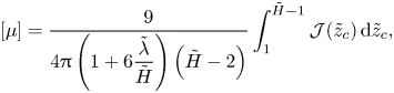 \begin{equation} [\mu] = \frac{9}{\displaystyle 4{\rm \pi}\left(1+6\frac{ \tilde{\lambda}}{ \tilde{H}} \right) \left( \tilde{H}-2\right)} \int_1^{ \tilde{H}-1} {\mathcal{J}}( \tilde{z}_{c})\, \textrm{d} \tilde{z}_{c}, \end{equation}
where the integrand  ${\mathcal {J}}( \tilde{z}_{c})$ contains a stresslet part ${\mathcal {J}}_S( \tilde{z}_{c})$ and a quadrupole part ${\mathcal {J}}_Q( \tilde{z}_{c})$:
 \begin{gather} {\mathcal{J}}( \tilde{z}_{c}) = {\mathcal{J}}_S( \tilde{z}_{c})+ {\mathcal{J}}_Q( \tilde{z}_{c}), \end{gather}
 \begin{gather} {\mathcal{J}}_S( \tilde{z}_{c})= \left( 1 -2 \frac{ \tilde{z}_{c}}{ \tilde{H}} \right) \tilde{S}_{xz} , \quad {\mathcal{J}}_Q( \tilde{z}_{c})= -\frac{1}{ \tilde{H}} \tilde{Q}_{xzz} . \end{gather}
3. Expressions of stresslet and quadrupole
This section is concerned with the contributions of interactions with walls in the calculation of the intrinsic viscosity and then in the calculation of the stresslet component  $S_{xz}$ and quadrupole component $Q_{xzz}$ for a freely moving sphere in the ambient flow field (2.1) with coefficients (2.3a,b).
3.1. Interactions based on individual walls
In general, the hydrodynamic interactions of the sphere with both slipping walls should be taken into account. As stated in the introduction, this is a difficult task. Indeed, for various calculation methods such as the boundary element method (BEM) (see Pozrikidis Reference Pozrikidis1992; Sellier Reference Sellier, Aliabadi and Wen2010) and the method of multipoles (see Bhattacharya, Bławzdziewicz & Wajnryb Reference Bhattacharya, Bławzdziewicz and Wajnryb2005a,Reference Bhattacharya, Bławzdziewicz and Wajnrybb; Ekiel-Jeżewska & Wajnryb Reference Ekiel-Jeżewska, Wajnryb, Feuillebois and Sellier2009) it would first require the derivation of the Green tensor between two parallel slip walls. This very challenging issue is left for future works.
For a large enough gap  $\tilde{H}$ between walls, in the case of no-slip walls, the earlier calculation by (I) has shown that the interactions of particles with the nearest wall give a good approximation to the effective viscosity, by comparison to the accurate multipole method which takes both walls simultaneously into account. For the case of a freely moving particle between no-slip parallel walls, the earlier study by Pasol et al. (Reference Pasol, Martin, Ekiel-Jeżewska, Wajnryb, Bawzdziewicz and Feuillebois2011) showed that the nearest wall approximation and the wall superposition approximation both gave excellent results for the particle velocity for a wide range of parameters. Based on these experiences, we consider here the following.
(i) The zero wall approximation, denoted as 0w, in which the stresslet and quadrupole in (2.26b,c) are calculated ignoring the interactions of the particle with the walls, that is (see (I))
(3.1a,b)and injected into the expression (2.26) for the integrand, to be denoted as\begin{equation} \tilde{S}_{xz, \textit{0w}} = \frac{10{\rm \pi}}{3} \left(1-\frac{2 \tilde{z}_{c}}{ \tilde{H}}\right) , \quad \tilde{Q}_{xzz, \textit{0w}} = -\frac{8{\rm \pi}}{3 \tilde{H}} , \end{equation}${\mathcal {J}}_ \textit {0w}$; the result for the intrinsic viscosity calculated with (2.25) is then denoted as $[\mu ]_ \textit {0w}$.(ii) The nearest wall approximation, denoted as nw, in which the stresslet and quadrupole in (2.26b,c) are calculated by considering interactions with the nearest wall only; the integrand is then denoted as
${\mathcal {J}}_ \textit {nw}$ and the intrinsic viscosity $[\mu ]_ \textit {nw}$ is calculated by integration using (2.25). By symmetry of ${\mathcal {J}}_ \textit {nw}$ with respect to the channel mid-plane, a simpler formula is
(3.2)\begin{equation} [\mu]_ \textit{nw} = \frac{9}{\displaystyle 2{\rm \pi}\left(1+6\dfrac{\tilde{\lambda}}{ \tilde{H}} \right) \left( \tilde{H}-2\right)} \int_1^{ \tilde{H}/2} {\mathcal{J}}_ \textit{nw}( \tilde{z}_{c})\, \textrm{d} \tilde{z}_{c} . \end{equation}(iii) The wall superposition approximation, denoted as ws. In this case, consider first the influence of the wall at
$\tilde{z}_{c}=0$ over the whole gap (note that ${\mathcal {J}}_ \textit {1w}= {\mathcal {J}}_ \textit {nw}$ only for $1\leq \tilde{z}_{c} \leq \tilde{H}/2$). The integrand, denoted as ${\mathcal {J}}_ \textit {1w}( \tilde{z}_{c})$, here takes into account the interactions with the wall at $\tilde{z}_{c}=0$. Integrating ${\mathcal {J}}_ \textit {1w}( \tilde{z}_{c})$ for $\tilde{z}_{c}$ from $1$ to $\tilde{H}-1$ provides the resulting contribution to the intrinsic viscosity:
(3.3)\begin{equation} [\mu]_ \textit{1w} = \frac{9}{\displaystyle 4{\rm \pi}\left(1+6\dfrac{ \tilde{\lambda}}{ \tilde{H}} \right) \left( \tilde{H}-2\right)} \int_1^{ \tilde{H}-1} {\mathcal{J}}_ \textit{1w}( \tilde{z}_{c})\,\textrm{d} \tilde{z}_{c} . \end{equation}The calculation of the contribution of the second wall at
$\tilde{z}_{c}= \tilde{H}-1$ to the intrinsic viscosity is carried out in the same way. Without entering into detail, it is clear that both walls will give equal contributions. These contributions are then added. In this process, the common part for large distance from the wall should not be counted twice, thus we subtract the 0w case. Finally, the formula for the wall superposition approximation is
(3.4)in which\begin{equation} [\mu]_ \textit{ws} = 2\, [\mu]_ \textit{1w} - [\mu]_ \textit{0w} \end{equation}$[\mu ]_ \textit {0w}$ is calculated with (3.1a,b) and (2.25) as explained above. The integrand for this case is
(3.5)\begin{equation} {\mathcal{J}}_ \textit{ws} = 2\, {\mathcal{J}}_ \textit{1w} - {\mathcal{J}}_ \textit{0w} . \end{equation}


In any case (either nw or ws), the quantities required for averaging are the stresslet and quadrupole on a freely suspended sphere in the ambient flow (2.1) in the presence of a single slip wall. The bipolar coordinates method (BCM) will be used in this article to obtain very accurate results for these quantities. This borrows results from previous papers to be quoted below and also provides novel derivations for the quadrupole, for four basic flow fields presented in § 3.2. Then § 3.3 presents the new calculation of the quadrupole for a sphere held fixed in ambient linear and quadratic shear flows.
3.2. Relevant normalized quantities
The vector  ${\boldsymbol {r}}_i$ in the stresslet operator (2.10) and quadrupole operator (2.11) is now for a single particle (dropping the $i$ subscript) denoted as ${\boldsymbol {r}}= {\boldsymbol {x}}- {\boldsymbol {x}}_C$, where ${\boldsymbol {x}}$ is a current point on the sphere and ${\boldsymbol {x}}_C$ is the position of the sphere centre $C$ as measured from a point located on the lower wall $W_1$.
The translational and rotational velocities of a freely moving sphere in the flow field (2.1) are, by linearity of Stokes equations, respectively along  $x$, say $U_x$, and along $y$, say $\varOmega _y$. By linearity of Stokes equations, they are obtained as the superposition of the corresponding freely moving velocities in a laminar shear flow $k_1z$ (see Loussaief et al. Reference Loussaief, Pasol and Feuillebois2015) and in a quadratic shear flow $k_2z$ (see Ghalia et al. Reference Ghalia, Feuillebois and Sellier2016):
 \begin{gather} U_x = U^{s}_x + U^{q}_s,\quad\varOmega_y = \varOmega^{s}_y + \varOmega^{q}_y \end{gather}
 \begin{gather} \frac{U^{s}_x}{k_1(z_c+\lambda)}= u^{s}_x=\frac{\displaystyle\frac{1}{2( \tilde{z}_{c}+ \tilde{\lambda})} f^{r}_{xy}c^{s}_{yx} + f^{s}_{xx} c^{r}_{yy} } { f^{t}_{xx}c^{r}_{yy} - f^{r}_{xy}c^{t}_{yx}} , \end{gather}
 \begin{gather} \frac{ \varOmega^{s}_y}{k_1/2}= \omega^{s}_y=\frac{2( \tilde{z}_{c}+ \tilde{\lambda}) f^{s}_{xx}c^{t}_{yx} + f^{t}_{xx} c^{s}_{yx} } { f^{t}_{xx}c^{r}_{yy} - f^{r}_{xy}c^{t}_{yx}} , \end{gather}
 \begin{gather} \frac{U^{q}_x}{k_2\left(z_c+\dfrac{a^{2}}{3}\right)}= u^{q}_x= {{ \tilde{z}_{c}^{2} c_{yy}^{r}\, f_{xx}^{q}+ \tilde{z}_{c}\, f_{xy}^{r} c_{yx}^{q}}\over{[ \tilde{z}_{c}^{2}+\frac 13] [c_{yy}^{r}\, f_{xx}^{t}-f_{xy}^{r} c_{yx}^{t}]}}, \end{gather}
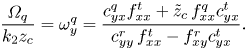 \begin{gather} {{ \varOmega_q}\over{k_2 z_c}}=\omega^{q}_y={{c_{yx}^{q} f_{xx}^{t}+ \tilde{z}_{c}\, f_{xx}^{q} c_{yx}^{t}}\over{c_{yy}^{r}\, f_{xx}^{t}-f_{xy}^{r} c_{yx}^{t}}}. \end{gather}
We here also define dimensionless velocities. The ‘ $f$'s and ‘ $c$'s on the right-hand sides are dimensionless friction coefficients which either have the limit of unity (when subscripts are identical) or vanish (when subscripts are different) when the sphere is infinitely far from the wall. The results (3.6c) and (3.6d) were obtained (in Loussaief et al. Reference Loussaief, Pasol and Feuillebois2015) by writing that the sums of forces and torques for a sphere translating and rotating in a fluid at rest and a sphere held fixed in a linear shear flow $k_1z$ vanish. Likewise, (3.6e) and (3.6d) were obtained (in Ghalia et al. Reference Ghalia, Feuillebois and Sellier2016) from vanishing total force and torque for the quadratic shear flow $k_2z$. Adding the results in (3.6a) and (3.6b) amounts to expressing the condition that the total force and torque in the flow field (2.1) vanish. By total force and torque, we mean those due to translation and rotation in a fluid at rest and particle held fixed in the flow fields $k_1z$ and $k_2z$.
Expressions for the normalized stresslet and quadrupole defined in (2.23) are displayed in table 1, in terms of dimensionless stresslet coefficients  $s^{\bullet }_{xz}$ and quadrupole coefficients $q^{\bullet }_{xzz}$, where the superscript bullet ( $\bullet$) represents $t, r, s$ and $q$ for translation, rotation, ambient linear shear flow and ambient quadratic shear flow, respectively. The coefficients $s^{\bullet }_{xz}$ and $q^{\bullet }_{xzz}$ for $(t, s, q)$ tend to unity for $\tilde{z}_{c}\to \infty$ whereas $s^{r}_{xz}$ and $q^{r}_{xzz}$ vanish (the coefficients $6{\rm \pi}$ and $8{\rm \pi}$ in the definitions of these last quantities are chosen arbitrarily).
Normalized stresslet and quadrupole (defined in (2.23)) for elementary flow fields: a translating sphere, a rotating sphere in a fluid at rest and a sphere held fixed in linear shear and quadratic shear flows.
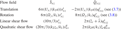
In the last column of table 1, the normalized quadrupoles  $q^{t}_{xzz}$ due to translation and $q^{r}_{xzz}$ due to rotation were obtained by applying the Lorentz reciprocity theorem (see appendix A):
 \begin{gather} q^{t}_{xzz} = 3 \tilde{z}_{c} \left( \tilde{z}_{c} + 2 \tilde{\lambda} \right) f^{t}_{xx} -6 \tilde{z}_{c} \left( \tilde{z}_{c} + \tilde{\lambda} \right) f^{s}_{xx}+3 \tilde{z}_{c}^{2}\, f^{q}_{xx}, \end{gather}
 \begin{gather} q^{r}_{xzz} = \frac 34 \tilde{z}_{c} \left( \tilde{z}_{c} + 2 \tilde{\lambda} \right) f^{r}_{xy}+ \tilde{z}_{c} c^{s}_{yx} - \tilde{z}_{c} c^{q}_{yx}. \end{gather}
All dimensionless coefficients, in these formulae and in table 1, except  $q^{s}_{xzz}$ and $q^{q}_{xzz}$, have been calculated previously using bipolar coordinates for a sphere interacting with a slip plane wall. The results of Loussaief et al. (Reference Loussaief, Pasol and Feuillebois2015) and Ghalia et al. (Reference Ghalia, Feuillebois and Sellier2016) will be used here. For instance, the dimensionless stresslet coefficient for translation, $s^{t}_{xz}$, is obtained from earlier results as follows:
(i) From (2.23a) and the first line, first column in table 1, the stresslet component due to translation is
$S_{xz}^{t}=6{\rm \pi} \mu _0 aU_x s^{t}_{xz}$, which is the original definition of $s^{t}_{xz}$ in Ghalia etal. (Reference Ghalia, Feuillebois and Sellier2016) (see (66) there).(ii) In Ghalia et al. (Reference Ghalia, Feuillebois and Sellier2016), (B 4a–c) gives
$s^{t}_{xz}$ in terms of coefficients $B_n^{t}, C_n^{t}, E_n^{r}$.(iii) These coefficients appear in the expressions of harmonics (describing the flow field) as series in bipolar coordinates (see (3.3) in Loussaief et al. (Reference Loussaief, Pasol and Feuillebois2015));
$B_n^{t}, C_n^{t}$ are for the translation problem and $E_n^{r}$ is for the rotation problem. These coefficients are calculated accurately in bipolar coordinates in Loussaief et al. (Reference Loussaief, Pasol and Feuillebois2015).


The determination of the novel coefficients  $q^{c}_{xzz}$ and $q^{q}_{xzz}$ is the topic of the next subsection.
The expressions of the stresslet and quadrupole for translation and rotation in table 1 are valid for any translation velocity  $U_x$ and rotational velocity $\varOmega _y$, respectively. Consider now a freely moving sphere in the flow field (2.1) (with (2.3a,b)). Its translational and rotational velocities are obtained by adding the contributions of the linear and quadratic shear flows shown in (3.6):
 \begin{gather} U_x=k_1(z_c+\lambda)u^{s}_x+ k_2\left(z_c^{2}+\frac{a}{3}\right)u^{q}_x, \quad \varOmega_y=\frac{k_1}{2} \omega^{s}_y + k_2 z_c \omega^{q}_y. \end{gather}
These expressions are then introduced in table 1. The stresslet and quadrupole for a freely moving sphere in the flow field (2.1) are obtained as superpositions of those for a sphere translating and rotating in a fluid at rest and those for a sphere held fixed in the shear flows  $k_1z$ and $k_2z$:
 \begin{align} \tilde{S}_{xz} &= 6{\rm \pi} \left[ \left( \tilde{z}_{c}+ \tilde{\lambda}\right) u^{s}_x -\frac{1}{ \tilde{H}} \left( \tilde{z}_{c}^{2}+\frac 13 \right) u^{q}_x \right] s^{t}_{xz}, \nonumber\\ &\quad +6{\rm \pi} \left[ \frac{1}{2} \omega^{s}_y -\frac{ \tilde{z}_{c}}{ \tilde{H}} \omega^{q}_y \right] s^{r}_{xz} +\frac{10{\rm \pi}}{3} s^{s}_{xz} -\frac{20{\rm \pi}}{3} \frac{ \tilde{z}_{c}}{ \tilde{H}} s^{q}_{xz}, \end{align}
 \begin{align} \tilde{Q}_{xzz} &= -2{\rm \pi} \left[ \left( \tilde{z}_{c}+ \tilde{\lambda}\right) u^{s}_x -\frac{1}{ \tilde{H}} \left( \tilde{z}_{c}^{2}+\frac 13 \right) u^{q}_x \right] q^{t}_{xzz} \nonumber\\ &\quad +8{\rm \pi} \left[ \frac{1}{2} \omega^{s}_y -\frac{ \tilde{z}_{c}}{ \tilde{H}} \omega^{q}_y \right] q^{r}_{xzz} +2{\rm \pi} \left( \tilde{z}_{c}+ \tilde{\lambda}\right) q^{s}_{xzz} -2{\rm \pi} \frac{ \tilde{z}_{c}^{2}}{ \tilde{H}} q^{q}_{xzz} . \end{align}
3.3. Determination of the normalized quadrupoles $q^{s}_{xzz}$ and $q^{q}_{xzz}$


The reader only interested in the results for the effective viscosity may skip this subsection and go directly to § 3.4.
We derive here the normalized quadrupoles  $q^{s}_{xzz}$ and $q^{q}_{xzz}$ (recall table 1) for a sphere, with radius $a$ and centre $O',$ held fixed near the $z=0$ plane slip wall in an ambient linear or quadratic shear flow $({\boldsymbol {u}}_a,p_a)$ with stress tensor $\boldsymbol {\sigma }_a$. The disturbance flow $({\boldsymbol {u}}',p')$ about the sphere has stress tensor $\boldsymbol {\sigma }'$ and it is recalled that the sphere distance to the wall is $z_c>a$ while the wall slip length is $\tilde{\lambda} a.$ The quadrupole $Q_{xzz}$, exerted by the disturbed flow on the sphere, is $Q_{xzz}=Q^{a}_{xzz}+Q^{d}_{xzz}$ with
 \begin{equation} Q^{a}_{xzz}=\int[{\boldsymbol{e}}_x\boldsymbol{\cdot}{} \boldsymbol{\sigma}_a\boldsymbol{\cdot}{\boldsymbol{n}}](z-z_c)^{2}\,\textrm{d}S,\quad Q^{d}_{xzz}=\int[{\boldsymbol{e}}_x\boldsymbol{\cdot} \boldsymbol{\sigma}'\boldsymbol{\cdot}{\boldsymbol{n}}](z-z_c)^{2}\,\textrm{d}S. \end{equation}
From the definitions (2.23) and table 1, it follows that the dimensionless quadrupoles  $q_{xzz}^{s}$ and $q_{xzz}^{q}$ are defined by
 \begin{gather} Q_{xzz}=2{\rm \pi}\mu_0 k_1 a^{4}( \tilde{z}_{c}+\tilde{\lambda})q^{s}_{xzz}\quad \textrm{for} \ {\boldsymbol{u}}_a={\boldsymbol{u}}_s:=k_1(z+a\tilde{\lambda}){\boldsymbol{e}}_x\ \textrm{and}\ p_a=0, \end{gather}
 \begin{gather} Q_{xzz}=2{\rm \pi}\mu_0 k_2 a^{3} z_c^{2}q^{q}_{xzz}\quad \textrm{for}\ {\boldsymbol{u}}_a={\boldsymbol{u}}_q:=k_2 z^{2}{\boldsymbol{e}}_x\ \textrm{and}\ p_a=2\mu_0 k_2 x. \end{gather}
Let us now derive the integrals in (3.12a,b). Following the original idea suggested by Dean & O'Neill (Reference Dean and O'Neill1963) for a sphere rotating parallel to a no-slip wall, it is convenient to use spherical polar coordinates  $(r,\theta ,\varphi )$ with the sphere centre as the origin and $r=O'M, x=r\sin \theta \cos \varphi , y=r\sin \theta \sin \varphi , z=z_c+r\cos \theta .$ Here $\theta$ and $\varphi$ run in $[0,{\rm \pi} ]$ and $[0,2{\rm \pi} ],$ respectively. In addition, the disturbance velocity ${\boldsymbol {u}}'$ polar components are $(u'_r,u'_{\theta },u'_{\varphi }).$ On the $r=a$ sphere surface $S,$ with unit normal ${\boldsymbol{n}}=\boldsymbol{O}'\boldsymbol{M}/a$, we write for convenience of calculation ${\boldsymbol {e}}_x\boldsymbol {\cdot } \boldsymbol {\sigma }'\boldsymbol {\cdot }{\boldsymbol {n}}=\mu _0(T_1+T_2)$ with
 \begin{gather} aT_1=\cos\theta\cos\varphi\left[\left({\frac{\partial u'_r}{\partial\theta}}\right)-u'_{\theta}\right] +\sin\varphi[u'_{\varphi}]-{\frac{\sin\varphi}{\sin\theta}} \left({\frac{\partial u'_r}{\partial\varphi}}\right), \end{gather}
 \begin{gather} T_2=\left[2\left(\frac{\partial u'_r}{\partial r}\right)- \frac{p'}{\mu_0}\right]\sin\theta\cos\varphi +\cos\theta\cos\varphi\left({\frac{\partial u'_{\theta}}{\partial r}}\right) -\sin\varphi\left({\frac{\partial u'_{\varphi}}{\partial r}}\right). \end{gather}
The contribution of  $T_e$ for $e=1,2$ to the quadrupole $Q^{d}_{xzz}$ is denoted $Q^{d,e}_{xzz}$. On the sphere boundary $(z-z_c)^{2}\,\textrm {d}S=a^{4}[\cos \theta ]^{2}\sin \theta \,\textrm {d}\theta \,\textrm {d}\varphi$ and ${\boldsymbol {u}}'=-{\boldsymbol {u}}_a$. Using (3.15) easily gives
 \begin{equation} Q^{a}_{xzz}=Q^{d,1}_{xzz}=0\quad \textrm{if}\ {\boldsymbol{u}}_a={\boldsymbol{u}}_s, \quad (Q^{a}_{xzz},Q^{d,1}_{xzz})={\frac{8{\rm \pi}\mu_0k_2 a^{5}}{5}}\left({\frac{2}{3}},{\frac{1}{7}}\right) \ \textrm{if}\ {\boldsymbol{u}}_a={\boldsymbol{u}}_q. \end{equation}
The calculation of  $Q^{d,2}_{xzz}$ is tricky. It employs the cylindrical coordinates $(\rho ,z,\varphi )$ with $\rho =\{x^{2}+y^{2}\}^{1/2}$ being the distance to the $(O,{\boldsymbol {e}}_z)$ axis. The cylindrical components, $(v_{\rho },v_z,v_{\varphi })$, of the disturbance velocity ${\boldsymbol {u}}'$ satisfy
 \begin{equation} u'_r=\sin\theta[v_{\rho}]+\cos\theta[v_z],\quad u'_{\theta}=\cos\theta[v_{\rho}]-\sin\theta[v_z],\quad u'_{\varphi}=v_{\varphi}. \end{equation}
The relations (3.18a–c) provide the following expressions for the radial derivatives of  $(u'_r,u'_{\theta },u'_{\varphi }),$ required in (3.16) (note that $\theta$ is kept constant in these derivatives):
 \begin{gather} \displaystyle{\frac{\partial u'_r}{\partial r}}= \sin\theta\left({\frac{\partial v_{\rho}}{\partial r}}\right) +\cos\theta\left({\frac{\partial v_z}{\partial r}}\right), \end{gather}
 \begin{gather} \displaystyle{\frac{\partial u'_{\theta}}{\partial r}} = \cos\theta\left({\frac{\partial v_{\rho}}{\partial r}}\right) -\sin\theta\left({\frac{\partial v_z}{\partial r}}\right),\quad {\frac{\partial u'_{\varphi}}{\partial r}}={\frac{\partial v_{\varphi}}{\partial r}}. \end{gather}
For each considered ambient velocity field, either  ${\boldsymbol {u}}_a^{s}$ (linear shear) or ${\boldsymbol {u}}_a^{q}$ (quadratic shear), the disturbance flow $({\boldsymbol {u}}',p')$ about the sphere is written (see e.g. Ghalia et al. Reference Ghalia, Feuillebois and Sellier2016)
 \begin{gather} v_{\rho}=\frac{1}{2}\left\{\frac{{\rho} Q_1}{c}+U_0+U_2\right\} \cos\phi,\quad v_{\phi}={\frac{1}{2}} (U_2-U_0)\sin\phi, \end{gather}
 \begin{gather} v_z=\frac{1}{2}\left\{\frac{zQ_1}{c}+2W_1\right\}\cos\phi, \quad p'=\mu_0 Q_1\cos\phi,\quad c=(z_c^{2}-a^{2})^{1/2}, \end{gather}
with functions  $W_1, U_0, U_1$ and $U_2$ solely depending upon $(\rho ,z)$ (or equivalently upon $(r,\theta$)). Injecting (3.19a–c)–(3.21a–c) into (3.16) provides, by elementary manipulations not detailed here for conciseness,
 \begin{align} Q^{d,2}_{xzz}&=\mu_0\int_S a^{2} T_2[\cos\theta]^{2}\,\textrm{d}S={\rm \pi}\mu_0 a^{4}\int_0^{{\rm \pi}}\tilde{T}_2 [\cos\theta]^{2}\sin\theta \,\textrm{d}\theta,\end{align}
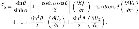 \begin{align} \tilde{T}_2&={\frac{\sin\theta}{\sinh\alpha}} \left[1+{\frac{\cosh\alpha\cos\theta}{2}}\right] \left({\frac{\partial Q_1}{\partial r}}\right)+ \sin\theta\cos\theta\left({\frac{\partial W_1}{\partial r}}\right)\nonumber\\ &\quad +\left[1+{\frac{\sin^{2}\theta}{2}}\right] \left({\frac{\partial U_0}{\partial r}}\right) +{\frac{\sin^{2}\theta}{2}}\left({\frac{\partial U_2}{\partial r}}\right). \end{align}
In finding the disturbance flow, it is more convenient to determine the functions  $W_1, U_0, U_1$ and $U_2$ in terms of the bipolar coordinates $(\xi ,\eta )$ which are related to $(\rho ,z)$ as follows (see e.g. Happel & Brenner Reference Happel and Brenner1973):
 \begin{equation} \rho=\frac{c\sin\eta}{\cosh\xi-\cos\eta},\quad z=\frac{c\sinh\xi}{\cosh\xi-\cos\eta},\quad c=(z_c^{2}-a^{2})^{1/2}. \end{equation}
For each angle  $\varphi$ the liquid domain above the slip wall is obtained taking $0\leq \eta \leq {\rm \pi}$ and $0\leq \xi \leq \alpha$ with $\alpha >0$ given by $\cosh \alpha = \tilde{z}_{c}.$ In the $(\xi ,\eta ,\varphi )$ coordinates the $\xi =0$ and $\xi =\alpha$ surfaces are the slip $z=0$ plane wall and the sphere boundary, respectively. It is then found (see Ghalia et al. Reference Ghalia, Feuillebois and Sellier2016) that
 \begin{gather} W_1(\xi,\eta)=k_lc^{l}(\cosh\xi-t)^{1/2}\sin\eta\sum_{n\geq 1}A_n\sinh( \gamma_n\xi) P'_n(t), \end{gather}
 \begin{gather} Q_1(\xi,\eta)=k_lc^{l}(\cosh\xi-t)^{1/2}\sin\eta\sum_{n\geq 1}[B_n\cosh(\gamma_n\xi) +C_n\sinh(\gamma_n\xi)]P'_n(t), \end{gather}
 \begin{gather} U_0(\xi,\eta)=k_lc^{l}(\cosh\xi-t)^{1/2}\sum_{n\geq 0}^{\infty}[D_n\cosh(\gamma_n\xi) +E_n\sinh(\gamma_n\xi)]P_n(t), \end{gather}
 \begin{gather} U_2(\xi,\eta)=k_lc^{l}(\cosh\xi-t)^{1/2}\sin^{2}\eta\sum_{n\geq 2}[F_n\cosh(\gamma_n\xi) +G_n\sinh(\gamma_n\xi)]P''_n(t), \end{gather}
with  $c=a\sinh \alpha , \gamma _n=n+1/2, t=\cos \eta , P_n$ the usual Legendre polynomial of order $n$ and primes designating differentiations. In (3.25)–(3.28) the superscript $l$ that is either $l=1$ or $l=2$ refers to either the ambient linear shear flow or quadratic shear flow, respectively. The dimensionless coefficients $A_n, B_n, C_n, D_n, E_n, F_n$ and $G_n$ in (3.25)–(3.28) are required to vanish as $n$ becomes infinite. They are obtained by enforcing the condition ${{\nabla }}\boldsymbol {\cdot }{\boldsymbol {u}}'=0$ in the $0\leq \xi \leq \alpha$ liquid domain, the Navier slip and impermeability conditions on the $\xi =z=0$ slip wall and the no-slip condition ${\boldsymbol {u}}'=-{\boldsymbol {u}}_a$ on the $\xi =\alpha$ sphere surface (see details in Loussaief et al. (Reference Loussaief, Pasol and Feuillebois2015) and Ghalia et al. (Reference Ghalia, Feuillebois and Sellier2016)).
Recall that in (3.23) the partial derivatives with respect to  $r$ are to be performed at constant angle $\theta .$ Then (see also Dean & O'Neill Reference Dean and O'Neill1963), on the $\xi =\alpha$ sphere boundary
 \begin{align} \left({\frac{\partial f}{\partial r}}\right) & ={\frac{t-\cosh\alpha}{c}} \left({\frac{\partial f}{\partial \xi}}\right), \quad \textrm{d}\theta={\frac{\sin\theta \,\textrm{d}\eta}{\sin\eta}}, \end{align}
 \begin{align} \sin\theta & ={\frac{\sinh\alpha\sin\eta}{\cosh\alpha-t}},\quad \cos\theta={\frac{t\cosh\alpha-1}{\cosh\alpha-t}}, \end{align}
with  $t=\cos \eta$ and $\partial f/\partial \xi$ to be taken at constant value of $\eta$ for $f(r,\theta )=f(\xi ,\eta )$. Appealing to (3.29a–d) when using (3.22)–(3.23) then finally yields
 \begin{align} Q^{d,2}_{xzz}/\mu_0=\int_S a^{2} T_2[\cos\theta]^{2} \,\textrm{d}S=-{\frac{{\rm \pi} k_l a^{2} c^{l+1}} {4}}\{S_A+S_B+S_C+S_D+S_E+S_F+S_G\}, \end{align}
where  $S_L$ designates a sum involving the coefficients $L$ introduced in (3.25)–(3.28). Each sum $S_L$ is expressed in terms of 10 integrals $I_m(n,\alpha )$ in appendix B. For example,
 \begin{equation} S_A=\sinh\alpha\sum_{n\geq 1}\left\{\sinh\alpha[1-\textrm{e}^{-2\gamma_n\alpha}]I_4(n,\alpha) +2\gamma_n[1+\textrm{e}^{-2\gamma_n\alpha}]I_3(n,\alpha)\right\}A_n \end{equation}
with the definitions
 \begin{equation} I_m(n,\alpha)=\textrm{e}^{\gamma_n\alpha}\int_{-1}^{1}\frac{(1-t^{2})[(\cosh\alpha)t-1]^{3} P'_{n}(t)\,\textrm{d}t}{(\cosh\alpha-t)^{m+3/2}}\quad \textrm{for}\ m=3,4. \end{equation}
Appendix B both defines and explains how to calculate analytically all 10 integrals  $I_m$. Since they are too lengthy to be reproduced in this article, formulae are displayed only for $I_3$ and $I_4$ in appendix B while the analytical results for the other integrals $I_m$ are given in the supplementary material available at https://doi.org/10.1017/jfm.2020.429. Finally, combining (3.17) with (3.30) provides the quadrupole $Q_{xzz}=Q^{a}_{xzz}+Q^{d,1}_{xzz}+Q^{d,2}_{xzz}$ for the ambient linear and quadratic shear flows. Using (3.13) and (3.14) then gives the desired coefficients $q^{s}_{xzz}$ and $q^{q}_{xzz}$.
3.4. Accuracy issues and comparisons against a BEM approach
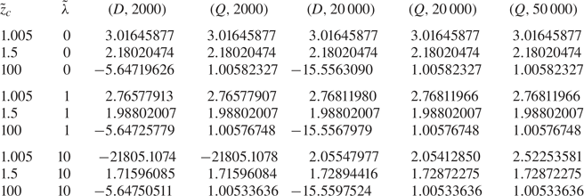
The BCM is known to be very accurate provided its numerical implementation is adequately handled. The encountered series, as in (3.25)–(3.28), are truncated beyond a given integer  $N_t$. Of course, the value of $N_t$ required to ensure a given accuracy level depends on $(z_z/a,{\tilde{\lambda} })$. Moreover, while coding in Fortran double precision $(D)$ was sufficient for some domains of parameters (see Ghalia et al. Reference Ghalia, Feuillebois and Sellier2016), it has been found here necessary to code in Fortran quadruple precision $(Q)$ (as in Loussaief et al. Reference Loussaief, Pasol and Feuillebois2015) to accurately compute the new terms $q^{s}_{xzz}$ or $q^{q}_{xzz}$ when $\tilde{z}_{c}$ becomes large whatever ${\tilde{\lambda} }\geq 0.$ Moreover, the quadruple precision code uses another numerical method, i.e. the Thomas algorithm (as in Loussaief et al. Reference Loussaief, Pasol and Feuillebois2015), instead of the classical LU factorization (as in Ghalia et al. Reference Ghalia, Feuillebois and Sellier2016) to invert the tridiagonal matrix providing the series coefficients. The interest of the Thomas algorithm is that it allows the calculation of more terms in the series at a reduced cost in memory and CPU calculation time. Displaying results using these two different methods also provides here a supplementary check for the validity of the numerical results. The comparison is illustrated for $q^{q}_{xzz}$ in table 2 taking $z_z/a=1.005, 1.5, 100$ and ${\tilde{\lambda} }=0,1,10$. Clearly, for $z_z/a=100$ the calculations in quadruple precision are more accurate and efficient (smaller required value of $N_t$) whatever ${\tilde{\lambda} }.$ For instance, taking $N_t=2000$ in quadruple precision is sufficient to reach an eight-digit accuracy when $z_z/a=100$ even for the large slip case ${\tilde{\lambda} }=10$. When the sphere is very close to a wall with large slip length it is necessary to take $N_t$ large for computations in both double and quadruple precision.
Normalized quadrupole  $q^{q}_{xzz}$ computed with the BCM using either Fortran double precision $(D)$ or quadruple precision with the Thomas algorithm $(Q)$ and truncating the series in (3.25)–(3.28) beyond $N_t$. For example, the column $(D,2000)$ gathers the values of $q^{q}_{xzz}$ computed in Fortran double precision taking $N_t=2000$.
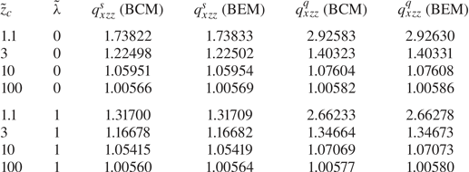
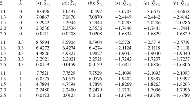
In view of the great amount of calculations (see the previous subsection, appendix B and the supplementary material), it is useful for validation to compare the BCM predictions, for both dimensionless quadrupoles  $q^{s}_{xzz}$ and $q^{q}_{xzz},$ with the ones obtained by the quite different BEM implemented in Ghalya, Sellier & Feuillebois (Reference Ghalya, Sellier and Feuillebois2012) for a solid arbitrary-shaped particle interacting with the $z=0$ slip wall. This method uses the Green tensor fulfilling the boundary conditions on the wall and implements six-node (P2 quadratic approximation) isoparametric curved triangular meshes on the particle surface. More details can also be found in Sellier (Reference Sellier, Aliabadi and Wen2010). Some numerical comparisons for $q^{s}_{xzz}$ and $q^{q}_{xzz}$ are displayed in table 3 for a few settings $(z_z/a,{\tilde{\lambda} })$ and taking $N_t=20\,000$ for the BCM (with quadruple precision) and $1058$ nodal points on the sphere boundary for the BEM. Since the BEM requires much more refined meshes on the sphere surface as $\tilde{z}_{c}-1$ vanishes the results in table 3 are given for $\tilde{z}_{c}\geq 1.1.$ As observed in table 3, a very good agreement (up to a four-digit accuracy) is found between the BEM and the quadruple precision BCM (with the Thomas algorithm). Finally, comparisons between the BCM and BEM techniques are given in table 4 for the key quantities $\tilde{S}_{xz}$ and $\tilde{Q}_{xzz}$ taking $H=5a.$ Again, a good agreement is observed.
Computed normalized quadrupoles  $q^{s}_{xzz}$ and $q^{q}_{xzz}$ using either the BCM with $N_t=20\,000$ or the BEM spreading $1058$ collocation nodal points on the sphere surface.
Computed normalized quantities  $\tilde{S}_{xz}$ and $\tilde{Q}_{xzz}$ using the BEM ( $\star$ symbol) or the BCM taking either $N_t=2000$ (a) or $N_t=20\,000$ (b). Here $H=5a$ and $1058$ collocation nodal points are distributed on the sphere surface for the BEM.
4. Numerical results
This section presents the numerical results obtained for the intrinsic viscosity and its dependence in terms of the slip length when attention is restricted, as discussed in the introduction, to the widely encountered range  $\tilde{\lambda} \leq 1.$ It contains four subsections. First, a comparison with earlier results obtained in (I) for the case of no-slip walls is presented in § 4.1. Then, for a slip wall, values of the integrands (see § 3.1) appearing in the expressions for the intrinsic viscosity are presented in detail in § 4.2. Comprehensive results for the intrinsic viscosity are displayed in § 4.3. Finally, numerical results for the intrinsic viscosity are fitted with a polynomial and the resulting interpolation formula is displayed in § 4.4.
Throughout this section, calculations were performed in quadruple precision Fortran, using, as in Loussaief et al. (Reference Loussaief, Pasol and Feuillebois2015), the Thomas algorithm for the calculation of the terms of series in bipolar coordinates. The number  $N_t$ of terms of the truncated series is adjusted, depending on $( \tilde{z}_{c}, \tilde{\lambda})$, to obtain a 15-digit accuracy.
4.1. Comparison and validation for no-slip walls
The intrinsic viscosity for no-slip walls was calculated in (I) using the accurate multipole method which fully takes into account the interactions with both walls. That method was corrected for lubrication to speed up the convergence rate. Plots in (I) were in terms of the dimensionless ratio  $H/d= \tilde{H}/2$. We use also $H/d$ in this article for comparison with (I) and also for all further plots. This choice is also motivated by possible comparisons with experiments in which the particle diameter is provided rather than the radius. A comparison was made in (I) with a ‘simplified model’ which took into account only the stresslet term and in this case only the nearest wall. That comparison clearly showed that both models match for $H/d\geq 10$ while the behaviour is quite different for $H/d$ down to unity. Indeed, the intrinsic viscosity predicted by the ‘simplified model’ drops down to zero for $H/d\to 1$.
The calculation of the quadrupole term in bipolar coordinates, presented in § 3.3, will be used here. First, the full nearest-wall model nw which takes into account both the stresslet and the quadrupole is employed. The comparison is shown in figure 3. It is observed that the curves for the two-walls exact model (say tw) and the nw model have the same shape for small  $H/d,$ which is not the case when only stresslet is taken into account (compare with figure 2 in (I)). It is also observed that the value of $[\mu ]$ for the nw model is smaller than that for the two-walls model. This is expected, since some friction effects from both walls at the same time are discarded by the nw model, especially in the middle of the gap. For comparison, figure 3 also displays the results for the no-wall (0w) approximation already shown in (I).
Comparison and validation for no-slip walls. Results for two walls (tw) are from (I) and were calculated for two parallel walls with the multipole method. The wall superposition (ws, dash-dotted line, red) and nearest wall (nw, lines with larger dots, blue) results are obtained with the present bipolar coordinates calculations. The no wall (0w, lines with circles) curves are obtained from the analytical equations (3.1a,b). Dashed lines for the various models (see legend) are for stresslet only. The horizontal dotted line at  $[\mu ]=2.5$ recalls the result of Einstein (Reference Einstein1906) for the intrinsic viscosity in unbounded fluid.
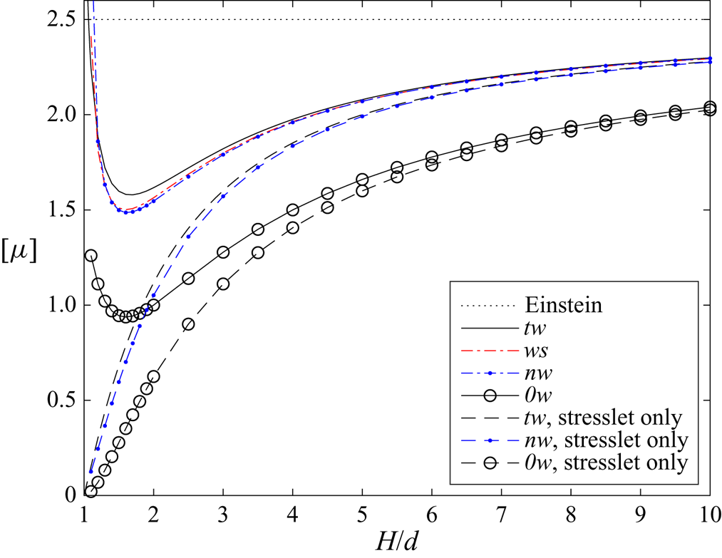
Results for the wall-superposition (ws) model, taking into account both the stresslet and quadrupole in the interaction with each wall separately, are also plotted in figure 3. Curves for the nw and ws models are remarkably close together in the range  $H/d\geq 1.2$.
The ability of the nw and ws models to predict the effective viscosity is quantified by considering their relative ‘error’  $({\rm \Delta} [\mu ])/[\mu ]$ by comparison with the exact tw model. For instance for the nw model, $({\rm \Delta} [\mu ])/[\mu ]= |1-[\mu ]_{nw}/[\mu ]_{tw}|$. These errors are plotted in figure 4. They are small and of comparable magnitude, the ws approximation being a little better that the nw one in the range $1.5 \leq H/d \leq 6$. In the same figure, we plot the horizontal dashed line which indicates the 5 % error level. It is remarkable that for both nw and ws approximations the relative error remains below that level in the wide range $H/d\geq 2$. For $H/d\geq 3$, both relative errors are even less than 2 %.
Comparison and validation for no-slip walls: relative differences between the nw and ws models and the exact two-walls (tw) results of Feuillebois et al. (Reference Feuillebois, Ekiel-Jeżewska, Wajnryb, Sellier and Bławzdziewicz2016), i.e.  $|1-[\mu ]_ \textit {nw}/[\mu ]_ \textit {tw}|$ and $|1-[\mu ]_ \textit {ws}/[\mu ]_ \textit {tw}|$.
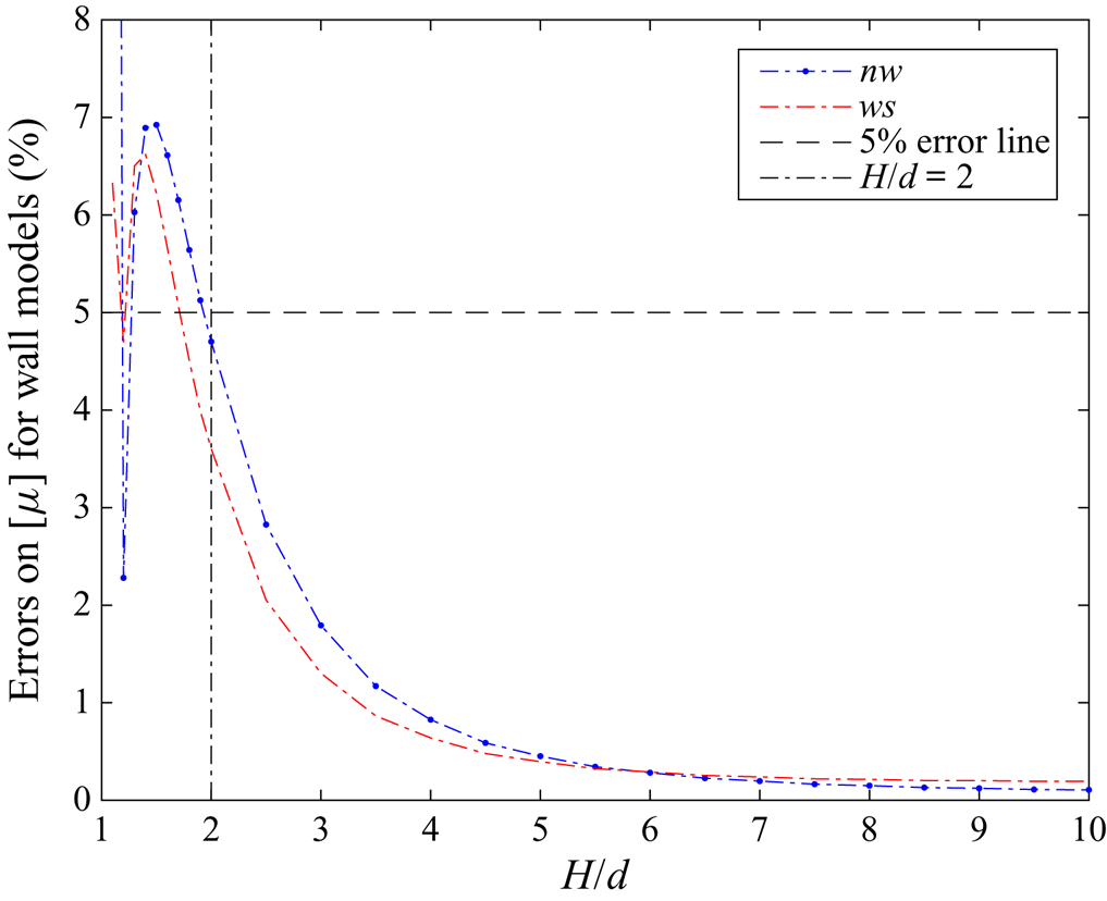
In conclusion, both nw and ws models are validated in the range  $H/d\geq 2$, this lower bound being represented as a vertical dash-dotted line in figure 4.
It is expected that the influences of walls decrease with increasing normalized slip length  $\tilde{\lambda}$. Consequently, for $\tilde{\lambda}>0$ the accuracy of both nw and ws models for slip walls is likely to be even better than 5 % in the whole range of distances $H/d\geq 2$.
The counterpart to restricting the domain to  $H/d\geq 2$ because of accuracy issues is that the interesting increase of $[\mu ]$ for small gaps due to lubrication (see figure 3) will not be reconsidered for slip walls. This is unavoidable in this article, since considering interactions with both walls at the same time would be compulsory for the range of small gaps $H/d< 2$; that is, using only lubrication with individual walls for $H/d$ close to unity would not be sufficient.
To make this idea more precise, consider first no-slip walls. For  $H/d$ close to unity, lubrication interactions with separate walls are of order $\log (H/d-1)$ and the next order term for small gaps (numerically very close to the first one) would include interactions with both walls, as pointed out in Ekiel-Jeżewska et al. (Reference Ekiel-Jeżewska, Wajnryb, Bawzdziewicz and Feuillebois2008). Using the precise multipole method (see Bhattacharya et al. Reference Bhattacharya, Bławzdziewicz and Wajnryb2005a,Reference Bhattacharya, Bławzdziewicz and Wajnrybb), it was shown there that the second-order lubrication terms (constant and of the same order as the leading logarithmic terms) are essentially different from the superposition of the corresponding single-wall terms.
This problem carries over to slip walls. When calculating the force on a sphere near a single slip wall, Davis, Kezirian & Brenner (Reference Davis, Kezirian and Brenner1994) found a weak log-singularity in the lubrication regime at low slip and no singularity for other values of the slip. A similar behaviour is expected for the stresslet and quadrupole. These quantities are actually calculated in this lubrication regime from our accurate bipolar coordinates results. As for the next order lubrication terms, they are expected to be numerically very close to the first-order ones and to involve both slip walls. These terms cannot be calculated at the present time.
4.2. Integrands in the expressions of the effective viscosity for slip walls
This subsection is concerned with the variations of the integrands  ${\mathcal {J}}_ \textit {0w}, {\mathcal {J}}_ \textit {nw}$ and ${\mathcal {J}}_ \textit {ws}$ (defined in § 3.1) in the expressions for the intrinsic viscosity and is motivated by twoissues:
(i) It is expected on physical grounds that the regions close to the slip walls would have a larger contribution than the region in the bulk of the channel and that these contributions would be more sensitive to variations in the slip length
$\tilde{\lambda}$.(ii) It was noticed for the no-slip case in figure 3 that the quadrupole term significantly contributes to the shape of the curve for the effective viscosity in the range
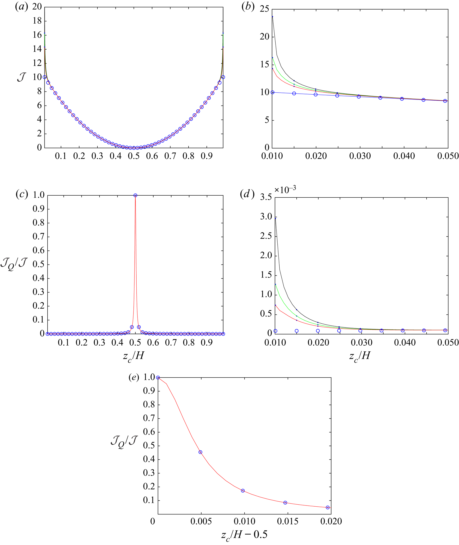
$H/d \leq 5$. This is an incentive for studying the relative contribution of the quadrupole to the integrand for the case of slip walls.


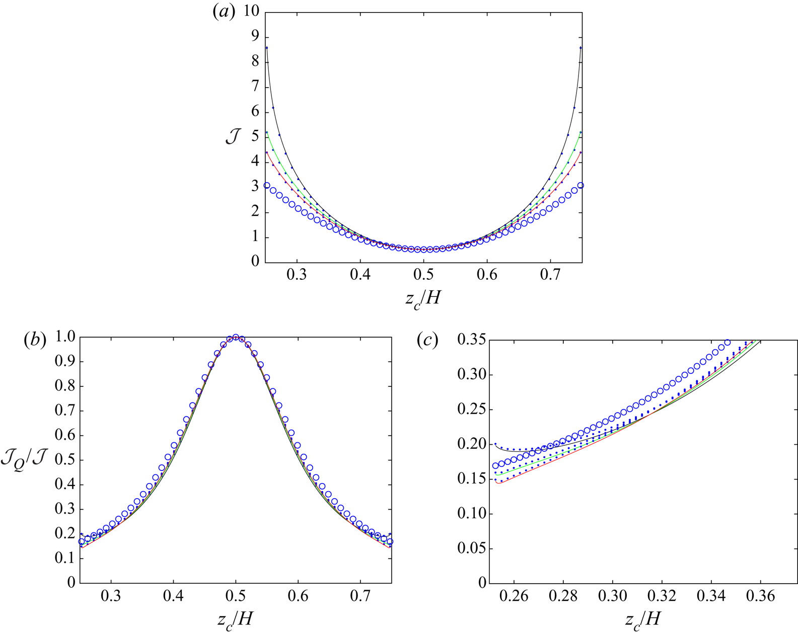
The integrands  ${\mathcal {J}}_ \textit {0w}$, ${\mathcal {J}}_ \textit {nw}$ and ${\mathcal {J}}_ \textit {ws}$ depend on $H/d, \tilde{\lambda}$ and $z_c/H$. We consider first the very confined case $H/d=2$. The integrands are plotted together versus $z_c/H$ in figure 5(a) for $\tilde{\lambda}=0, 0.3, 1$. It is observed that they are positive, symmetric with respect to the channel mid-plane and monotonic over each half-channel. Such a smooth behaviour allows calculation of the integral for the intrinsic viscosity by a standard Gauss–Legendre quadrature with 16 points on a half-channel. The smallest Gauss–Legendre integration point is at $z_c/H=0.2513$, not too close to the contact with wall at $z_c/H=0.2500$, i.e. higher than the lowest point $\tilde{z}_{c}=1.005$ considered in table 2, so that using $N_t\leq 20\,000$ in the bipolar coordinates calculations is sufficient for accuracy.
(a) Integrands  ${\mathcal {J}}_ \textit {0w}$, ${\mathcal {J}}_ \textit {nw}$ and ${\mathcal {J}}_ \textit {ws}$ (represented by circles, dots and solid lines, respectively) for the very confined case $H/d=2$. The sphere is in contact with a wall at $z_c/H=0.25$ and $z_c/H=0.75$. The integrands ${\mathcal {J}}_ \textit {nw}$ and ${\mathcal {J}}_ \textit {ws}$ look practically superimposed. Values of the normalized slip length $\tilde{\lambda}=0, 0.3$ and $1$ correspond to the upper, middle and lower solid lines (black, green and red), respectively. (b) Relative contribution of the quadrupole ${\mathcal {J}}_Q/ {\mathcal {J}}$ for the cases $\textit {0w}$, $\textit {nw}$ and $\textit {ws}$, with the same notation as in (a). (c) Zoom of the preceding plots near the wall, with the same notation as in (a).
Note that this integration procedure was already applied for the no-slip  $\tilde{\lambda}=0$ case in § 4.1.
The zero-wall integrand  ${\mathcal {J}}_ \textit {0w}$ (see figure 5a) is independent of $\tilde{\lambda}$ and always smaller than the other integrands. As expected, the contribution of the wall regions is larger than that of the bulk (say, of the domain $| \tilde{z}_{c}/H -0.5| \leq 0.15$). In the bulk region, each integrand is practically insensitive to $\tilde{\lambda}$. By contrast, ${\mathcal {J}}_ \textit {nw}$ and ${\mathcal {J}}_ \textit {ws}$ significantly decrease with increasing $\tilde{\lambda}$ in the wall regions. Moreover, ${\mathcal {J}}_ \textit {nw}$ and ${\mathcal {J}}_ \textit {ws}$ are very close together in the whole domain for all values of $\tilde{\lambda}$.
The relative contribution of the quadrupole term  ${\mathcal {J}}_Q/ {\mathcal {J}}$ (recall (2.26b,c)) is displayed in figure 5(b), still for $H/d=2$ and $\tilde{\lambda}=0, 0.3, 1$. It is larger than 15% and nearly insensitive to $\tilde{\lambda}$ in the bulk region. It varies slightly with $\tilde{\lambda}$ in the wall regions, as shown by the zoom in figure 5(c).
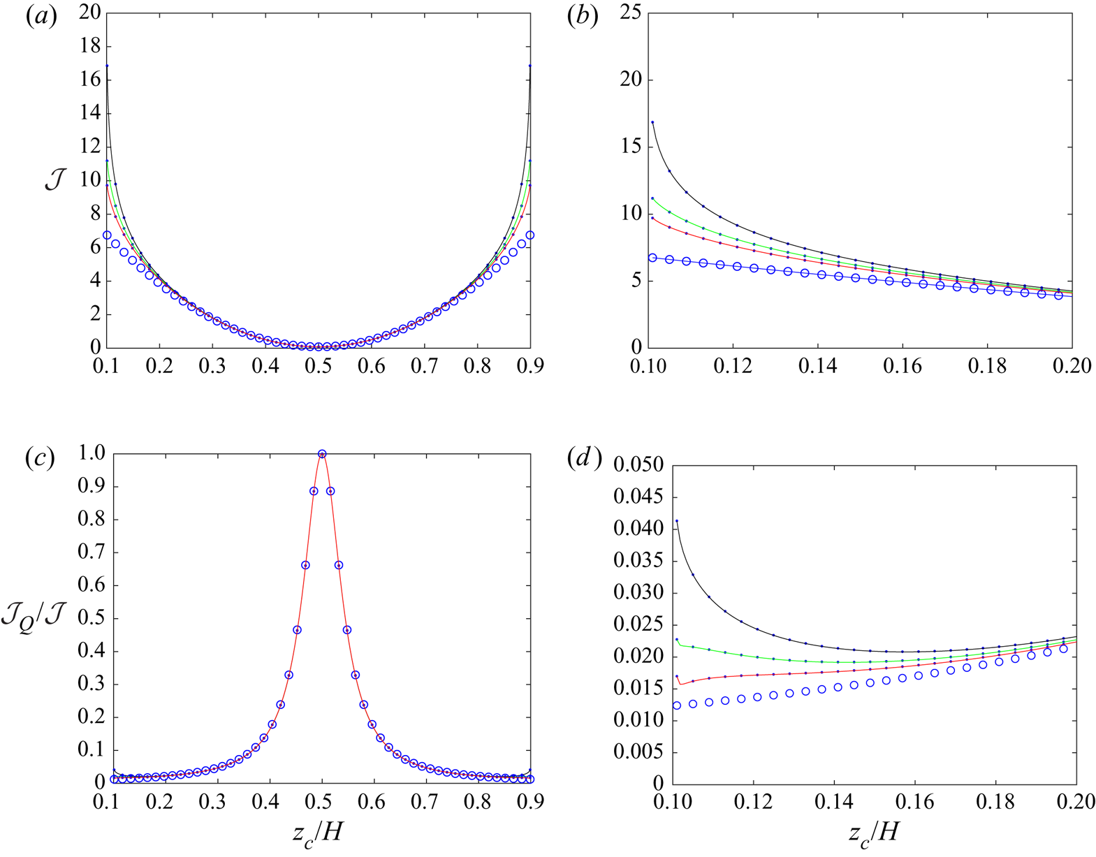
The influence of increasing the normalized channel width  $H/d$ is investigated in figure 6 for $H/d=5$ (moderately confined case) and in figure 7 for $H/d=50$ (widely separated walls), for comparison with figure 5 for $H/d=2$. The bulk region referred to above increases with $H/d$. Near the walls, the sensitivity of ${\mathcal {J}}$ to $\tilde{\lambda}$ is about the same for all values of $H/d$. The quadrupole part ${\mathcal {J}}_Q/ {\mathcal {J}}$ decays significantly as $H/d$ increases, except in the very vicinity of the channel mid-plane. Note that ${\mathcal {J}}_Q/ {\mathcal {J}}=1$ at mid-channel, i.e. $z_c/H= \tilde{z}_{c}/ \tilde{H}=1/2$, because the local shear rate $1-2 \tilde{z}_{c}/ \tilde{H}$ and thus also ${\mathcal {J}}_S$, see (2.26b,c), vanishes there. On the other end, as $H/d$ increases, the sensitivity of ${\mathcal {J}}_Q/ {\mathcal {J}}$ to $\tilde{\lambda}$ is enhanced near walls.
(a) Variation of the integrand  ${\mathcal {J}}_ \textit {0w}, {\mathcal {J}}_ \textit {nw}, {\mathcal {J}}_ \textit {ws}$. (b) Zoom of (a) near the wall at $z_c=0$. Curves are for the moderately confined case $H/d=5$. The sphere is in contact with a wall at $z_c/H=0.1$ and $z_c/H=0.9$. Values of the normalized slip length $\tilde{\lambda}=0$, 0.3 and 1 correspond to the upper, middle and lower solid lines (black, green and red), respectively. (c)Ratios ${\mathcal {J}}_{ \textit {0w},Q}/ {\mathcal {J}}_{ \textit {0w}}, {\mathcal {J}}_{ \textit {nw},Q}/ {\mathcal {J}}_{ \textit {nw}}, {\mathcal {J}}_{ \textit {ws},Q}/ {\mathcal {J}}_{ \textit {ws}}$. (d) Zoom of (c) near the wall at $z_c=0$.
(a) Variation of the integrand  ${\mathcal {J}}_ \textit {0w}, {\mathcal {J}}_ \textit {nw}, {\mathcal {J}}_ \textit {ws}$. (b) Zoom of (a) near the wall at $z_c=0$. Curves are for widely separated walls, $H/d=50$. The sphere is in contact with a wall at $z_c/H=0.01$ and $z_c/H=0.99$. Values of the normalized slip length $\tilde{\lambda}=0$, 0.3 and 1 correspond to the upper, middle and lower solid lines (black, green and red), respectively. (c)Ratios ${\mathcal {J}}_{ \textit {0w},Q}/ {\mathcal {J}}_{ \textit {0w}}, {\mathcal {J}}_{ \textit {nw},Q}/ {\mathcal {J}}_{ \textit {nw}}, {\mathcal {J}}_{ \textit {ws},Q}/ {\mathcal {J}}_{ \textit {ws}}$. (d) Zoom of (c) near the wall at $z_c=0$. (e) Zoom of the peak near the channel mid-plane.
4.3. Results for the effective viscosity for slip walls
We now present results for the effective viscosity of a dilute suspension of spheres bounded by two parallel impermeable slip walls, in the ranges  $H/d \geq 2$ and $0 \leq \tilde{\lambda} \leq 1$.
Recall from (2.25) that the suspension intrinsic viscosity depends both on an integral and on the prefactor
 \begin{equation*} \frac{9}{\displaystyle 4{\rm \pi}\left(1+6\frac{ \tilde{\lambda}}{ \tilde{H}} \right) \left( \tilde{H}-2\right)} . \end{equation*}
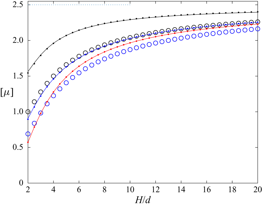
Consequently, the intrinsic viscosity for the zero-wall model varies with  $\tilde{\lambda}$ as $(1+6 \tilde{\lambda}/ \tilde{H})^{-1}$. This variation is illustrated for $\tilde{\lambda}=0.3$ and compared with the nw and the ws approximations in figure 8 (these approximations give very close results). Importantly, the intrinsic viscosity varies significantly from no-slip walls to slip walls in the whole range of $H/d$ represented here, even for this relatively small value $\tilde{\lambda}=0.3$. Moreover, comparing the 0w results to either the nw or the ws results shows that the influence of walls decays for increasing $\tilde{\lambda}$, as expected.
Intrinsic viscosity  $[\mu ]$ versus $H/d$. The nearest wall (nw) and wall superposition (ws) models are represented by dots and solid lines, respectively; they are practically superimposed. The top (black) dots and solid lines are for $\tilde{\lambda}=0$. The middle (blue) dots and solid lines are for $\tilde{\lambda}=0.3$ when taking into account the actual slip walls. The bottom (red) dots and solid lines are for $\tilde{\lambda}=0.3$ using the displaced no-slip walls model. The circle symbols ( $\circ$) represent the zero-wall model (0w): top (black), for $\tilde{\lambda}=0$; bottom (blue), for $\tilde{\lambda}=0.3$. The horizontal dotted line at 2.5 represents Einstein's result.
Since the predictions obtained by the  $\textit {nw}$ and ws models are very close we only report henceforth results given by the ws model.
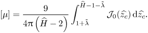
At this stage the above results make it possible to discuss the validity of the ‘displaced-walls’ model (see the introduction) if applied to the intrinsic viscosity  $[\mu ]=[\mu ]( \tilde{\lambda},H/d).$ Let $\widehat {H}$ be the normalized distance between the two fictitious displaced walls, that is, $\widehat {H}= \tilde{H}+2 \tilde{\lambda}$. The model for the intrinsic viscosity is obtained by
(i) first using (2.25) for no-slip walls separated by
$\widehat {H}$; let then $\widehat {z_c}$ denote the normalized position of a sphere centre with respect to the lower fictitious no-slip wall and ${\mathcal {J}}_0( \widehat {z_c})$ denote the value of the integrand (2.26) for the no-slip case;(ii) then restricting the integration range to the possible positions of particles in the gap
$\widehat {H}-2 \tilde{\lambda}$ between actual walls.


The resulting expression is
 \begin{equation} [\mu] = \frac{9}{\displaystyle 4{\rm \pi} \left( \widehat{H}-2\right)} \int_{1+ \tilde{\lambda}}^{ \widehat{H}-1- \tilde{\lambda}} {\mathcal{J}}_0( \widehat{z_c})\, \textrm{d} \widehat{z_c}. \end{equation}
Consider the example case  $\tilde{\lambda}=0.3$. From figure 8 it is observed that the lower dots (for nw) and line (for ws) (both red) representing the results of the ‘displaced-walls’ model are below the dots and line (both blue) results when actual slip walls are taken into account. The ‘displaced-walls’ model is very approximate for small gaps but becomes close to the correct result for large gaps. This feature is quantified in table 5 for a few values of $H/d.$ Thus, the ‘displaced-walls’ model is insufficient for predicting the intrinsic viscosity for small gaps.
Comparison for  $\tilde{\lambda}=0.3$ and $H/d=2,8,14,20$ (first column) of the intrinsic viscosity $[\mu ]$ obtained with the ‘displaced-walls’ model (second column) and for actual slip walls using the ws model (third column).
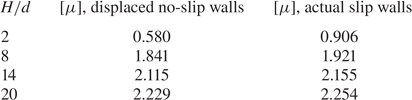
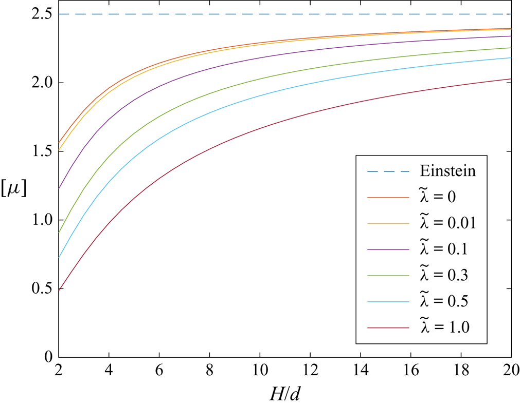
Figure 9, which represents the main result of this article, provides plots of the intrinsic viscosity for a comprehensive set of values of the normalized slip length in the range  $0 \leq \tilde{\lambda} \leq 1$ (even more data are provided in figure 13). For the largest slip length considered here, $\tilde{\lambda}=1$, in the very confined case $H/d=2$ the intrinsic viscosity $[\mu ]$ is divided by 3 compared with the no-slip case and divided by 5 compared with Einstein's result for the unbounded suspension. These ratios decrease only slowly with increasing $H/d$. Even for a very small slip length $\tilde{\lambda}=0.01$, there is a significant decrease of $[\mu ]$ in a large range of $H/d$ compared with the no-slip case. For given $H/d$, the intrinsic viscosity decreases with increasing slip length $\tilde{\lambda}$, as expected.
Variations of the intrinsic viscosity  $[\mu ]$ calculated with the ws model versus $H/d$ for various values of $\tilde{\lambda}$: from top to bottom, $\tilde{\lambda}=0, 0.01, 0.1, 0.3, 0.5, 1.0$.
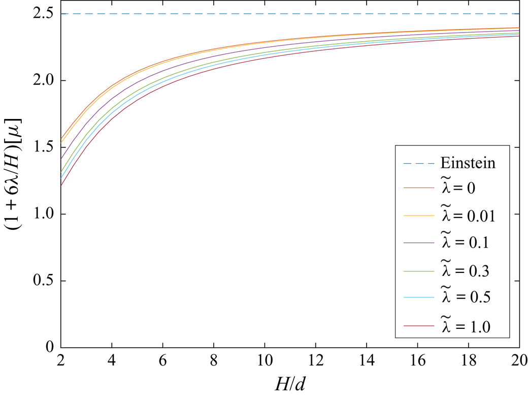
The dependence on  $\lambda$ in (2.25) comes on the one hand from the $1/(1+6\,\lambda /H)$ factor and on the other hand from the dependences on $\lambda$ of the stresslet and quadrupole in the average. Figure 10 shows a plot of $(1+6\,\lambda /H)[\mu ]$ versus $H/d$ for various values of $\lambda$. It is observed that all curves are significantly closer together than in figure 9. This proves that the factor $1/(1+6\,\lambda /H)$ is responsible for the largest part of the dependence on $\lambda$.
Variations of the product  $(1+6\,\lambda /H)[\mu ]$ calculated with the ws model versus $H/d$ for various values of $\tilde{\lambda}$: from top to bottom, $\tilde{\lambda}=0, 0.01, 0.1, 0.3, 0.5, 1.0$.
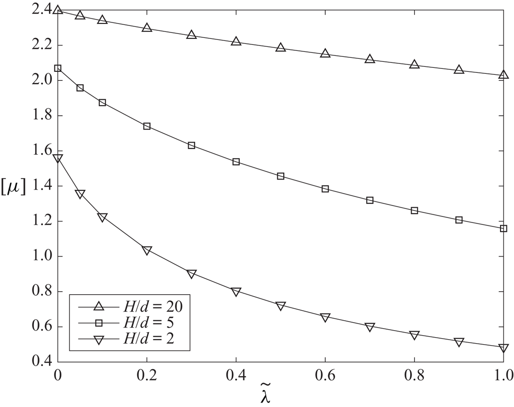
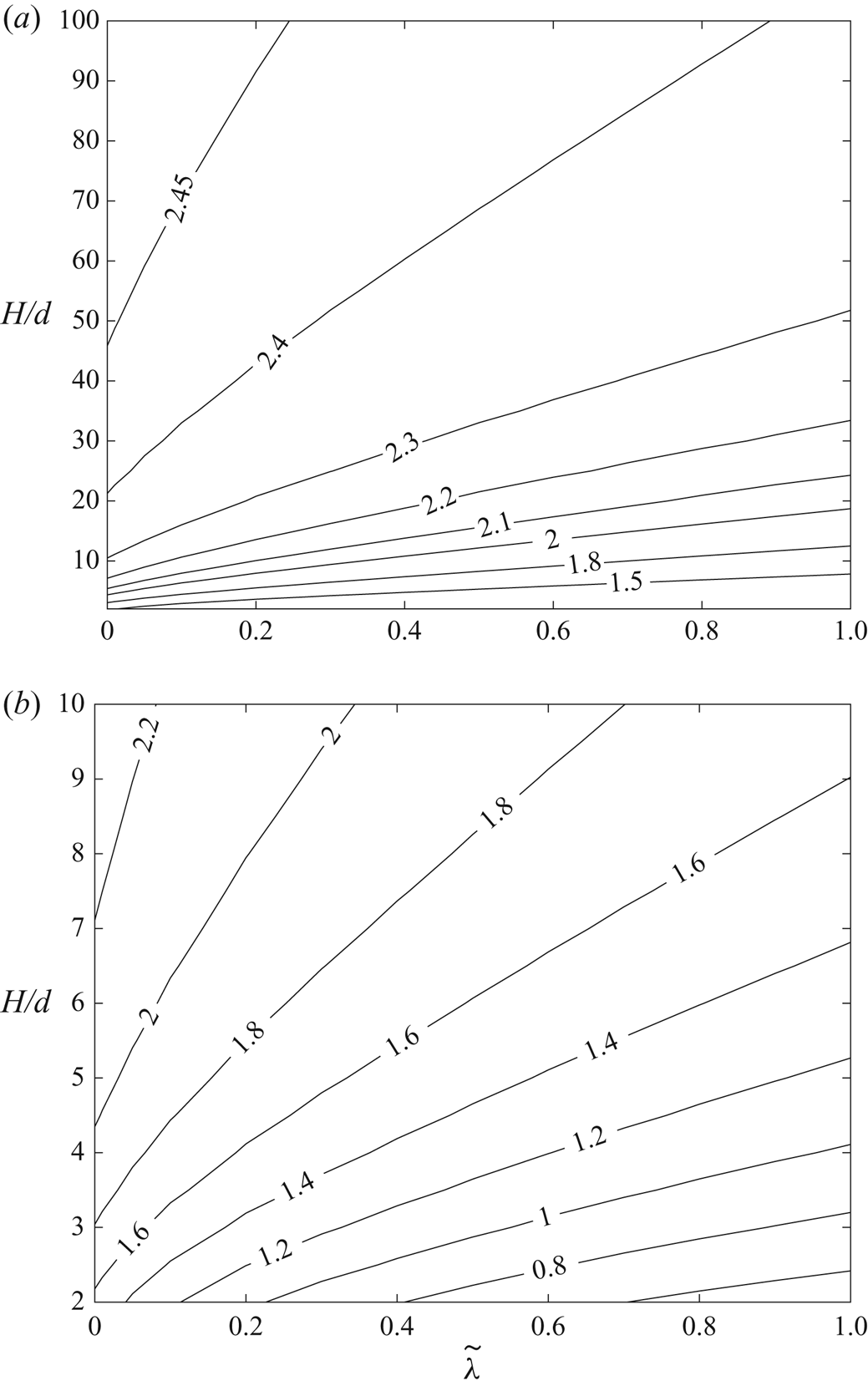
In figure 11, the variations of the intrinsic viscosity are plotted versus the slip length  $\tilde{\lambda}$ for the very confined case ( $H/d=2$), for the moderately confined case ( $H/d=5$) and for separated walls ( $H/d=20$). It is observed that for a given dilute suspension, the same intrinsic viscosity may be obtained with different sets of values ( $\tilde{\lambda},H/d$) (see also the contour plot in figure 14a).
Variations of the intrinsic viscosity  $[\mu ]$ with $\tilde{\lambda}$ for $H/d=2, 5, 20,$ calculated with the ws model (calculated points shown as symbols are here connected by straight lines).
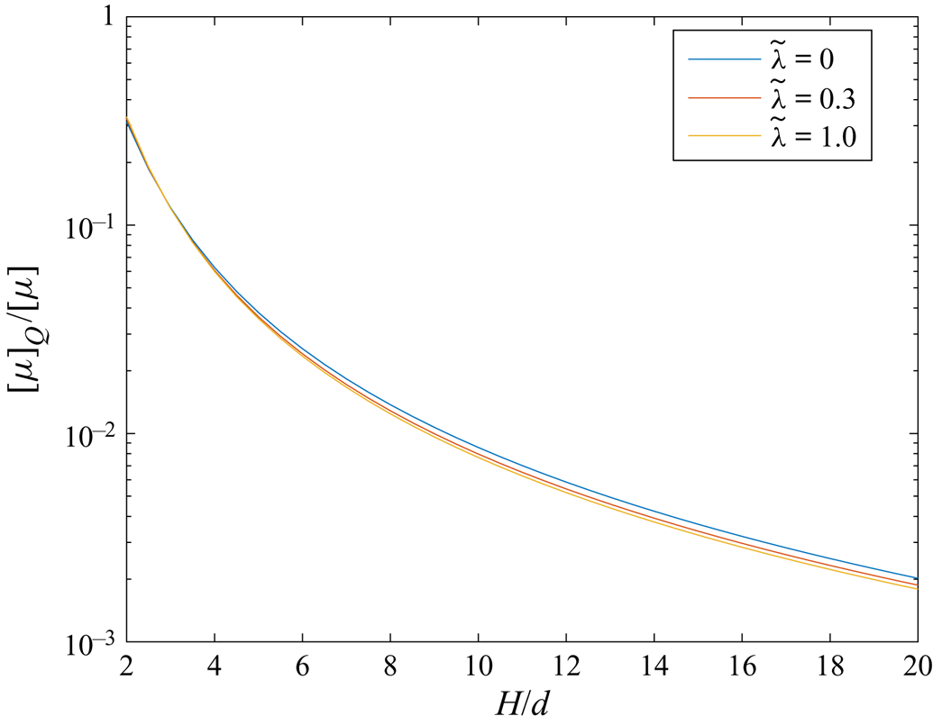
Finally, for comparison with figure 3 we plot for  $\tilde{\lambda}=0,0.3,1$ in figure 12 the contribution of the quadrupole term to the intrinsic viscosity $[\mu ]$ as the ratio $[\mu ]_Q/[\mu ],$ where $[\mu ]_Q$ is obtained by switching off the stresslet contribution in (2.24). This contribution is quite significant for small gaps, say $2\leq H/d \leq 4$. For $\tilde{\lambda}=0$, it becomes less than 5 % for $H/d> 4.4$. It appears that the ratio $[\mu ]_Q/[\mu ]$ is practically insensitive to the slip length $\tilde{\lambda}$, in the range considered here.
Relative contribution of the quadrupole term to the intrinsic viscosity versus  $H/d$ for $\tilde{\lambda}=0,0.3,1.0$ (as calculated with the ws model).
4.4. An interpolation formula for the effective viscosity
The preceding numerical results were obtained from a lengthy quadruple precision Fortran code enforcing the bipolar coordinates calculations. Building this code required substantial efforts. For a practical prediction of the effective viscosity, we therefore propose a handy and accurate formula interpolating our results obtained with the ws model.
Considering that  $[\mu ]$ has the Einstein limit of $5/2$ at $H/d\to \infty$ for any $\tilde{\lambda}$, it is convenient to fit, in the sense of least squares, the numerical results for $[\mu ]-5/2$ with a polynomial in $d/H$ and $\tilde{\lambda}$ as follows:
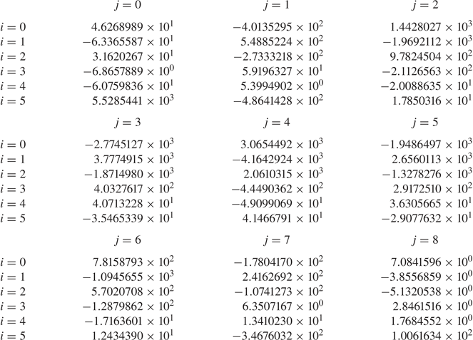
 \begin{equation} [\mu]_{\textit{fit}} = {\frac{5}{2} }-\sum_{i=0}^{5} \sum_{j=0}^{8} c_{i,j} \left( \frac dH \right)^{5-i} \tilde{\lambda}^{8-j} . \end{equation}
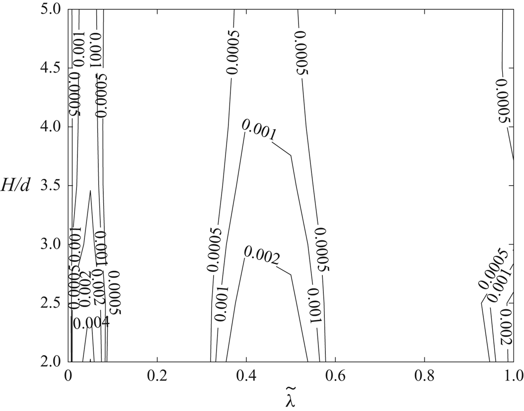
The selected upper bounds  $(5$ for $i$ and $8$ for $j$) were chosen as a compromise between a reasonable number of coefficients $c_{i,j}$ and a sufficient relative accuracy of at most $0.5\,\%$ (see later in figure 15). This value is consistent with expected accuracy of the $\textit {nw}$ and $\textit {ws}$ approximations.
We used (4.2) for fitting the numerical results for  $[\mu ],$ given by the ws model, up to $H/d=100$ and added, from physical considerations, the value $[\mu ]=5/2$ at $d/H=0$ for all values of $\tilde{\lambda}$. Moreover, even though the range of slip lengths $\tilde{\lambda}\leq 1$ was kept for physical reasons (see above), calculated values of $[\mu ]$ in the range $1 < \tilde{\lambda}\leq 2$ were used to improve the fitting precision of the polynomial in the range $0\leq \tilde{\lambda}\leq 1$. The coefficients $c_{i,j}$ of the fitting polynomial are displayed in table 6.
Coefficients  $c_{i,j}$ of the polynomial in formula (4.2) fitting the numerical results obtained with the ws model.
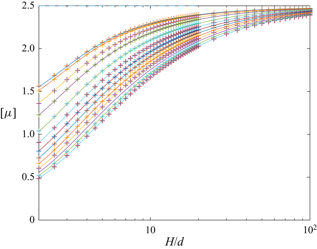
Results for  $[\mu ]$ using the fitting formula (4.2) are displayed as solid lines and compared to the exact results displayed as crosses in figure 13. Values for $[\mu ]$ are also shown as a contour plot in figure 14(a) and a zoom in the range $2\leq H/d \leq 10$ is provided in figure 14(b). Values of the relative error between the fitted and exact results are displayed in figure 15. Only values $H/d\leq 5$ are represented in this latter figure in order to show details of the relative error contour lines (for $H/d$ from $5$ to $100$ the contour lines become nearly parallel to the $\tilde{\lambda}=0$ vertical axis). It is remarked that, as discussed after (4.2), the error is mostly smaller than 0.4 %, except for small $\tilde{\lambda}$ and $H/d$ close to 2 where it is less than 0.5 % (this contour line is very close to $H/d=2$ in figure 15). For $H/d>3.5$, the error is smaller than 0.2 % for all values of $\tilde{\lambda}$.
Variations of the intrinsic viscosity  $[\mu ]$ (as predicted with the ws model) with $H/d$ from 2 to 100, for (from top to bottom): $\tilde{\lambda}=0, 0.01, 0.05$ and $0.1$ to $1$ in steps of $0.1$. Crosses: exact results; solid lines: fitting formula (4.2).
(a) Contour plot of the variations of the intrinsic viscosity  $[\mu ]$ with $\tilde{\lambda}$ and $H/d$ extracted from the exact results displayed in figure 13 (crosses). (b) Zoom plot for $2\leq H/d\leq 10$.
Contour plot of the relative error between the exact results and the fitted formula for  $[\mu ]$.
Finally, note that for the particular case  $\tilde{\lambda}=0$, the fitting formula (4.2) complements the results of (I) in the case of a suspension of spheres.
5. Discussion and conclusion
Two different models have been considered to apply the hydrodynamic interactions with one wall to the two-walls problem: the nearest-wall approximation and the wall-superposition approximation. These two approximations are consistent within 1 % (recall figure 4). For the no-slip case, they are within 5 % of the earlier exact results of Feuillebois et al. (Reference Feuillebois, Ekiel-Jeżewska, Wajnryb, Sellier and Bławzdziewicz2016) for two walls, when the gap is larger than two particle diameters.
The main result of the article is that the effective viscosity of a suspension  $\mu _{\textit{eff}}$, presented here in terms of the intrinsic viscosity $[\mu ]=( \mu _{\textit{eff}}-\mu _0)/(\mu _0 \phi )$, is very sensitive to the slip length on the walls. In the range of parameters considered here, a maximum decrease of the intrinsic viscosity by a factor of 3 is expected when the slip length $\lambda$ is equal to one particle radius and the gap between walls is equal to two particle diameters. Even for a small slip length of 0.01 particle radius, a significant decrease of a few percent of the viscosity is already predicted for the same gap. It has been shown that the quadrupole term has a significant contribution to the intrinsic viscosity $[\mu ],$ compared with the classical stresslet term, for narrow gaps (say $H/d\leq O(3)).$ Moreover, the relative contribution of the quadrupole term is very weakly dependent upon the normalized slip length $\tilde{\lambda}\leq 1$ (see figure 12). An outcome of our lengthy calculations is also a useful fitting formula (4.2) allowing a fast and accurate calculation of the intrinsic viscosity in the domain $2\leq H/d\leq 100$ and $\tilde{\lambda}\leq 1.$ Our results also show that the simple ‘displaced-walls’ model is not sufficient for predicting the effective viscosity.
From an experimental point of view, an appropriate set-up for measuring the effective viscosity of a dilute suspension would be the so-called microcapillary rheometer (see Vleminckx & Clasen (Reference Vleminckx and Clasen2014) and references therein). For comparing our predictions to experiment, the value of the wall slip length  $\lambda$ has to be known beforehand. If $\lambda$ is not known, a simple approach using (2.6) would be to first measure the head loss ${\rm \Delta} p_0$ and the volume flow rate ${\overline u}_0 H$ for the pure liquid (i.e. without particles) and then derive $\lambda .$ Then in a second step the experiment would be repeated for the dilute suspension thereby obtaining from (2.6) the experimental value of the effective viscosity $\mu_{\textit{eff}}.$ This latter value could then be compared to the one predicted using formula (4.2).
The nw and ws approximations have been found here to be quite appropriate for a dilute suspension of spheres; their results are also close together. These approximations might be relevant for non-spherical particles for some settings of the gap between walls and of the slip length. An essential ingredient is the calculation of the interaction between a non-spherical particle and a plane slip wall. An article reporting a study using a boundary formulation is presently in preparation, following the preliminary results of Ghalya et al. (Reference Ghalya, Sellier and Feuillebois2012).
Taking into account both slip walls at the same time is more difficult. This is especially true for narrow gaps. Our results are limited here to gaps  $H$ such that $H/d\geq 2$, because of our approach taking only single walls into account. Considering the proper effect of both walls would first require derivation of the Green tensor between two parallel slip walls. This result is presently not available. As discussed above, considering chains of spheres or other non-spherical particles, as was done by Feuillebois et al. (Reference Feuillebois, Ekiel-Jeżewska, Wajnryb, Sellier and Bławzdziewicz2015, Reference Feuillebois, Ekiel-Jeżewska, Wajnryb, Sellier and Bławzdziewicz2016) for no-slip walls, is also presently a challenge. Indeed, the Green tensor between two parallel slip walls is also needed here.
Finally, the present approach may be extended for a dilute suspension of spheres flowing between two parallel slip plane walls of unequal slip lengths. This topic, which requires substantial additional efforts, is postponed to future work.
Acknowledgments
A.S. and M.L.E.-J. benefited from the ITHACA project PPI/APM/2018/1/00045 financed by the Polish National Agency for Academic Exchange. M.L.E.-J. was supported in part by the National Science Centre under grant UMO-2018/31/B/ST8/03640.
Declaration of interests
The authors report no conflict of interest.
Supplementary material
Supplementary material is available at https://doi.org/10.1017/jfm.2020.429.
Appendix A. Determination of the normalized quadrupoles due to translation and rotation, i.e. $\boldsymbol{q}^{\boldsymbol{t}}_{\boldsymbol{xzz}}$ and $\boldsymbol{q}^{\boldsymbol{r}}_{\boldsymbol{xzz}}$


Consider a Stokes flow, with velocity  ${\boldsymbol {u}}$ and stress tensor $\boldsymbol {\sigma },$ about a sphere translating at a velocity $U_x{\boldsymbol {e}}_x$ and rotating at an angular velocity $\varOmega _y{\boldsymbol {e}}_y.$ Since $(z-z_c)^{2}=z_c(z_c+2\lambda )-2z_c(z+\lambda )+z^{2},$ the quadrupole component $Q_{xzz}$ (see (2.11)) exerted on the sphere surface becomes $Q_{xzz}=z_c(z_c+2\lambda )I_0+2z_c I_1-I_2$ with the integrals
 \begin{align} I_0=\int_S( \boldsymbol{\sigma}\boldsymbol{\cdot}{\boldsymbol{n}})\boldsymbol{\cdot}{\boldsymbol{e}}_x\,\textrm{d}S,\quad I_1=\int_S( \boldsymbol{\sigma}\boldsymbol{\cdot}{\boldsymbol{n}})\boldsymbol{\cdot}[-(z+\lambda){\boldsymbol{e}}_x]\,\textrm{d}S,\quad I_2=\int_S( \boldsymbol{\sigma}\boldsymbol{\cdot}{\boldsymbol{n}})\boldsymbol{\cdot}[-z^{2}{\boldsymbol{e}}_x]\,\textrm{d}S. \end{align}
Both integrals  $I_1$ and $I_2$ are determined using the Lorentz reciprocal identity (see Happel & Brenner Reference Happel and Brenner1973) and introducing the stresses $\boldsymbol {\sigma }_s$ and $\boldsymbol {\sigma }_q$ for the flow disturbances about the sphere when held fixed in the ambient either linear shear velocity $k_s(z+\lambda ){\boldsymbol {e}}_x$ or quadratic shear velocity $k_q z^{2}{\boldsymbol {e}}_x,$ respectively. It follows that
 \begin{equation} I_1=\int_S (\boldsymbol{\sigma}_s\boldsymbol{\cdot}{\boldsymbol{n}})\boldsymbol{\cdot}{\boldsymbol{u}}\,\textrm{d}S/k_s,\quad I_2=\int_S (\boldsymbol{\sigma}_q\boldsymbol{\cdot}{\boldsymbol{n}})\boldsymbol{\cdot}{\boldsymbol{u}}\,\textrm{d}S/k_q \end{equation}
in which on the sphere boundary  $S$ we have the condition ${\boldsymbol {u}}=U_x{\boldsymbol {e}}_x+ \varOmega _y{\boldsymbol {e}}_y\wedge {\boldsymbol {x}}'$, where ${\boldsymbol {x}}'$ is the vector pointing from the sphere centre to a point on its surface $S.$ Hence, (A 2a,b) yields
 \begin{gather} I_0=6{\rm \pi}\mu_0[a \varOmega_y f^{r}_{xy}-U_x\, f^{t}_{xx}],\quad I_1=2{\rm \pi}\mu_0 a[2a^{2} \varOmega_y c^{s}_{yx}-3(z_c+\lambda)U_x\, f^{s}_{xx}], \end{gather}
 \begin{gather} I_1=2{\rm \pi}\mu_0 a[4a^{3} \varOmega_y c^{q}_{yx}-3z_c^{2} U_x\, f^{q}_{xx}]\end{gather}
with the dimensionless friction coefficients  $f$ and $c$ introduced in Ghalia et al. (Reference Ghalia, Feuillebois and Sellier2016). Noting that, from (2.23) and table 1,
 \begin{equation} Q_{xzz}=-2{\rm \pi}\mu_0 U_x a^{3} q^{t}_{xzz}\quad \textrm{for}\ \varOmega_y=0, \quad Q_{xzz}=8{\rm \pi}\mu_0 \varOmega_y a^{4} q^{r}_{xzz}\quad \textrm{for}\ U_x=0 \end{equation}
Appendix B. Some among various integrals for the calculation of the quadrupole in linear and quadratic shear flows
The sums  $S_L$ occurring in (3.30) are expressed in terms of 10 integrals $I_m(n,\alpha )$ for positive integers $n\geq 0$ and $m=1,\ldots ,10.$ Setting $\gamma _n=n+1/2, X=\cosh \alpha -t$ and $g=[\cosh \alpha ]t-1,$ these integrals are defined as follows:
 \begin{equation} I_m(n,\alpha)=\textrm{e}^{\gamma_n\alpha}\int_{-1}^{1}f_m(t)\,\textrm{d}t, \end{equation}
where
 \begin{gather} f_1={\frac{(1-t^{2})g^{2} P'_{n}(t)}{X^{7/2}}},\quad f_2={\frac{(1-t^{2})g^{2} P'_{n}(t)}{X^{9/2}}},\quad f_3={\frac{(1-t^{2})g^{3} P'_{n}(t)}{X^{9/2}}}, \end{gather}
 \begin{gather} f_4={\frac{(1-t^{2})g^{3} P'_{n}(t)}{X^{11/2}}},\quad f_5={\frac{g^{2} P_{n}(t)}{X^{5/2}}},\quad f_6={\frac{g^{2} P_{n}(t)}{X^{7/2}}},\quad f_7={\frac{(1-t^{2})g^{2} P_{n}(t)}{X^{9/2}}}, \end{gather}
 \begin{gather} f_8={\frac{(1-t^{2})g^{2} P_{n}(t)}{X^{11/2}}},\quad f_9={\frac{(1-t^{2})^{2} g^{2} P''_{n}(t)}{X^{9/2}}},\quad f_{10}={\frac{(1-t^{2})^{2} g^{2} P''_{n}(t)}{X^{11/2}}}. \end{gather}
Then, in addition to (3.31) for the sum  $S_A,$ is has been found that
 \begin{align} S_B&=\sum_{n\geq 1}\left\{\sinh\alpha(1+\textrm{e}^{-2\gamma_n\alpha}) [I_2(n,\alpha)+\cosh\alpha I_4(n,\alpha)/2]\right.\nonumber\\ &\qquad +\left.\gamma_n(1-\textrm{e}^{-2\gamma_n\alpha})[2I_1(n,\alpha)+\cosh\alpha I_3(n,\alpha)]\right\}B_n,\end{align}
 \begin{align} S_C&=\sum_{n\geq 1}\left\{\sinh\alpha(1-\textrm{e}^{-2\gamma_n\alpha}) [I_2(n,\alpha)+\cosh\alpha I_4(n,\alpha)/2]\right.\nonumber\\ &\qquad \left.+\gamma_n(1+\textrm{e}^{-2\gamma_n\alpha})[2I_1(n,\alpha)+\cosh\alpha I_3(n,\alpha)]\right\}C_n, \end{align}
 \begin{align} S_D&=\sum_{n\geq 0}\left\{\sinh\alpha(1+\textrm{e}^{-2\gamma_n\alpha}) [I_6(n,\alpha)+(\sinh\alpha)^{2} I_8(n,\alpha)/2]\right.\nonumber\\ &\qquad \left.+\gamma_n(1-\textrm{e}^{-2\gamma_n\alpha}) [2I_5(n,\alpha)+\sinh^{2}\alpha I_7(n,\alpha)]\right\}D_n,\end{align}
 \begin{align} S_E&=\sum_{n\geq 0}\left\{\sinh\alpha(1-\textrm{e}^{-2\gamma_n\alpha}) [I_6(n,\alpha)+(\sinh\alpha)^{2} I_8(n,\alpha)/2]\right.\nonumber\\ &\qquad \left.+\gamma_n(1+\textrm{e}^{-2\gamma_n\alpha}) [2I_5(n,\alpha)+\sinh^{2}\alpha I_7(n,\alpha)]\right\}E_n,\end{align}
 \begin{align} S_F&=[\sinh^{2}\alpha]\sum_{n\geq 2}\left\{\sinh\alpha(1+\textrm{e}^{-2\gamma_n\alpha})I_{10}(n,\alpha)/2 +\gamma_n(1-\textrm{e}^{-2\gamma_n\alpha})I_9(n,\alpha)\right\}F_n, \end{align}
 \begin{align} S_G&=[\sinh^{2}\alpha]\sum_{n\geq 2}\left\{\sinh\alpha(1-\textrm{e}^{-2\gamma_n\alpha})I_{10}(n,\alpha)/2 +\gamma_n(1+\textrm{e}^{-2\gamma_n\alpha})I_9(n,\alpha)\right\}G_n. \end{align}
The integrals  $I_m$ are expressed in terms of 27 auxiliary integrals using the identity $g=[\cosh \alpha ]t-1.$ These new integrals are defined for integer $n\geq 0$ as
 \begin{gather}M_q^{v}(n,\alpha)=\textrm{e}^{\gamma_n\alpha}\int_{-1}^{1}{\frac{t^{q} P_n(t)\,\textrm{d}t}{X^{5/2+v}}} \quad \textrm{for}\ v=0,1\ \textrm{and}\ q=0,1,2; \end{gather}
 \begin{gather}M_l^{v}(n,\alpha)=\textrm{e}^{\gamma_n\alpha}\int_{-1}^{1}{\frac{t^{l} P_n(t)\,\textrm{d}t}{X^{5/2+v}}} \quad \textrm{for}\ v=2,3\ \textrm{and}\ l=0,1,2,3,4;\end{gather}
 \begin{gather}N_q^{1}(n,\alpha)=\textrm{e}^{\gamma_n\alpha}\int_{-1}^{1}{\frac{t^{q}(1-t^{2})P'_n(t)\,\textrm{d}t}{X^{5/2+v}}} \quad \textrm{for}\ q=0,1,2;\end{gather}
 \begin{gather}N_p^{v}(n,\alpha)=\textrm{e}^{\gamma_n\alpha}\int_{-1}^{1}{\frac{t^{p}(1-t^{2})P'_n(t)\,\textrm{d}t}{X^{5/2+v}}} \quad \textrm{for}\ v=2,3\ \textrm{and}\ p=0,1,2,3.\end{gather}
From Dean & O'Neill (Reference Dean and O'Neill1963) it appears that for  $n\geq 0$ and $\alpha >0$
 \begin{align}M^{0}_{0}(n,\alpha)={\frac{2\sqrt{2}(2n+1+2\coth\alpha)}{3(\sinh\alpha)^{2}}},\quad N^{1}_{0}(n,\alpha)={\frac{4\sqrt{2}n(n+1)}{15(\sinh\alpha)^{2}}}[2n+1+2\coth\alpha].\end{align}
Exploiting the identities (B 15a,b) and, for  $n\geq 1,$ the usual relations
 \begin{equation}tP_{n}(t)={\frac{(n+1)P_{n+1}(t)}{2n+1}}+{\frac{nP_{n-1}(t)}{2n+1}},\quad tP^{\prime}_{n}(t)={\frac{(n+1)P'_{n-1}(t)}{2n+1}}+{\frac{nP'_{n+1}(t)}{2n+1}}\end{equation}
make it possible to determine analytically the previous auxiliary integrals. Although elementary, the required manipulations are lengthy and the final results are given in the supplementary material. However, this appendix details the employed procedure for  $N^{2}_{q}$ and $N^{3}_{q}$ and also thereby (recall the definition $g=[\cosh \alpha ]t-1$) provides the integrals $I_3$ and $I_4$ from the relations
 \begin{align} I_{m+1}(n,\alpha)&=(\cosh\alpha)^{3} N^{m}_{3}(n,\alpha)-3(\cosh\alpha)^{2} N^{m}_{2}(n,\alpha)\nonumber\\ &\quad +3(\cosh\alpha)N^{m}_{1}(n,\alpha)-N^{m}_{0}(n,\alpha) \quad \textrm{for}\ m=2,3\ \textrm{and}\ n\geq 1. \end{align}
The integral  $N^{m}_{0}$ in (B 17) is immediately obtained by differentiating the second identity (B 15a,b) with respect to $\alpha$. The results are
 \begin{align} N_0^{2}(n,\alpha)&=\frac{4\sqrt{2}n(n+1)}{105(\sinh\alpha)^{5}} \left\{[(\cosh\alpha)^{2}](4n^{2}+4n+9)\right.\nonumber\\ &\quad \left.+\cosh\alpha\sinh\alpha(12n+6)-4n^{2}-4n+3\right\}, \end{align}
 \begin{align} N_0^{3}(n,\alpha)& =\frac{4\sqrt{2}n(n+1)}{945(\sinh\alpha)^{7}} \left\{(\cosh\alpha)^{3}](48n^{2}+48n+60)-\cosh\alpha(48n^{2}+48n-60)\right.\nonumber\\ &\quad +\sinh\alpha[(\cosh\alpha)^{2}](8n^{3}+12n^{2}+94n+45)\notag \\ & \quad - \left. \sinh\alpha(8n^{3}+12n^{2}-26n-15)\right\}. \end{align}
Using (B 18) and (B 19) and the second identity (B 16a,b) also first gives for  $n=1$
$n=1$
 \begin{align} N_2^{2}(1,\alpha)&=-8\textrm{e}^{3\alpha/2}\left\{\frac{96(\cosh\alpha)^{4}+336 (\cosh\alpha)^{3}+422(\cosh\alpha)^{2}+217\cosh\alpha+35} {105(\cosh\alpha+1)^{7/2}}\right.\nonumber\\ &\quad \left. -\frac{96(\cosh\alpha)^{4}-336(\cosh\alpha)^{3}+422(\cosh\alpha)^{2} -217\cosh\alpha+35}{105(\cosh\alpha-1)^{7/2}}\right\}, \end{align}
 \begin{align} N_3^{2}(1,\alpha)&=-8\textrm{e}^{3\alpha/2}\left\{\frac{320(\cosh\alpha)^{5}+ 1120(\cosh\alpha)^{4}+1388(\cosh\alpha)^{3}}{105(\cosh\alpha+1)^{7/2}}\right.\nonumber\\ &\quad +\frac{658(\cosh\alpha)^{2}+35\cosh\alpha-35}{105(\cosh\alpha+1)^{7/2}} +\frac{658(\cosh\alpha)^{2}-35\cosh\alpha-35}{105(\cosh\alpha-1)^{7/2}}\nonumber\\ &\quad \left. -\frac{320(\cosh\alpha)^{5}- 1120(\cosh\alpha)^{4}+1388(\cosh\alpha)^{3}}{105(\cosh\alpha-1)^{7/2}}\right\}, \end{align}
 \begin{align} N_2^{3}(1,\alpha)&=8\textrm{e}^{3\alpha/2}\left\{\frac{32(\cosh\alpha)^{4}+144(\cosh\alpha)^{3}+250(\cosh\alpha)^{2} +201\cosh\alpha+63}{115(\cosh\alpha+1)^{9/2}}\right.\nonumber\\ &\quad \left. -\frac{32(\cosh\alpha)^{4}-144(\cosh\alpha)^{3}+250(\cosh\alpha)^{2}-201\cosh\alpha+63} {115(\cosh\alpha-1)^{9/2}}\right\}, \end{align}
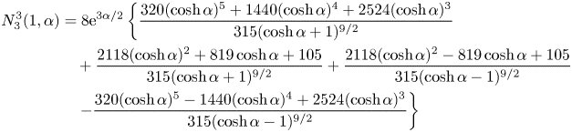 \begin{align} N_3^{3}(1,\alpha)&=8\textrm{e}^{3\alpha/2}\left\{\frac{320(\cosh\alpha)^{5}+ 1440(\cosh\alpha)^{4}+2524(\cosh\alpha)^{3}}{315(\cosh\alpha+1)^{9/2}}\right.\nonumber\\ &\quad +\frac{2118(\cosh\alpha)^{2}+819\cosh\alpha+105} {315(\cosh\alpha+1)^{9/2}}+\frac{2118(\cosh\alpha)^{2}-819\cosh\alpha+105} {315(\cosh\alpha-1)^{9/2}}\nonumber\\ &\left.\quad -\frac{320(\cosh\alpha)^{5}- 1440(\cosh\alpha)^{4}+2524(\cosh\alpha)^{3}}{315(\cosh\alpha-1)^{9/2}}\right\} \end{align}
and also for  $n=2$ the identities
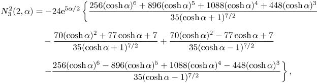 \begin{align} N_3^{2}(2,\alpha)&=-24\textrm{e}^{5\alpha/2} \left\{\frac{256(\cosh\alpha)^{6}+896(\cosh\alpha)^{5}+1088(\cosh\alpha)^{4}+448(\cosh\alpha)^{3}} {35(\cosh\alpha+1)^{7/2}}\right.\nonumber\\ &\quad -\frac{70(\cosh\alpha)^{2}+77\cosh\alpha+7}{35(\cosh\alpha+1)^{7/2}} +\frac{70(\cosh\alpha)^{2}-77\cosh\alpha+7}{35(\cosh\alpha-1)^{7/2}}\nonumber\\ &\left.\quad -\frac{256(\cosh\alpha)^{6}-896(\cosh\alpha)^{5} +1088(\cosh\alpha)^{4}-448(\cosh\alpha)^{3}}{35(\cosh\alpha-1)^{7/2}}\right\}, \end{align}
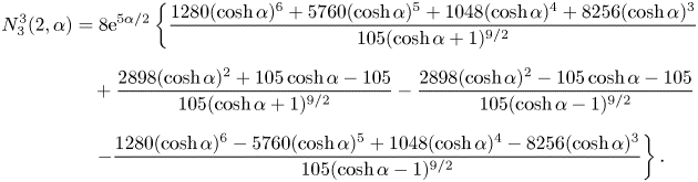 \begin{align} N_3^{3}(2,\alpha)&=8\textrm{e}^{5\alpha/2}\left\{ \frac{1280(\cosh\alpha)^{6}+5760(\cosh\alpha)^{5}+1048(\cosh\alpha)^{4}+8256(\cosh\alpha)^{3}} {105(\cosh\alpha+1)^{9/2}}\right.\nonumber\\ &\quad +\frac{2898(\cosh\alpha)^{2}+105\cosh\alpha-105}{105(\cosh\alpha+1)^{9/2}} -\frac{2898(\cosh\alpha)^{2}-105\cosh\alpha-105}{105(\cosh\alpha-1)^{9/2}}\nonumber\\ &\left.\quad -\frac{1280(\cosh\alpha)^{6}-5760(\cosh\alpha)^{5}+1048(\cosh\alpha)^{4}-8256(\cosh\alpha)^{3}} {105(\cosh\alpha-1)^{9/2}}\right\}. \end{align}
The same procedure finally provides for  $m=2,3$ the following recursion relationships:
 \begin{equation} N_1^{m}(n,\alpha)=\left(\frac{n+1}{2n+1}\right)N^{m}_{0}(n-1,\alpha)\textrm{e}^{\alpha}+ \left(\frac{n}{2n+1}\right)N^{m}_{0}(n+1,\alpha)\textrm{e}^{-\alpha} \quad \textrm{for}\ n\geq 1, \end{equation}
 \begin{equation}N_2^{m}(n,\alpha)=o_{n}N^{m}_{0}(n-2,\alpha)\textrm{e}^{2\alpha}+ p_{n}N^{m}_{0}(n,\alpha)+q_{n}N^{m}_{0}(n+2,\alpha)\textrm{e}^{-2\alpha} \quad \textrm{for}\ n\geq 2, \end{equation}
 \begin{align} N_3^{m}(n,\alpha)&=r_{n}N^{m}_{0}(n-3,\alpha)\textrm{e}^{3\alpha}+ s_{n}N^{m}_{0}(n-1,\alpha)\textrm{e}^{\alpha}\nonumber\\ &\quad +t_{n}N^{m}_{0}(n+1,\alpha)\textrm{e}^{-\alpha}+ u_{n}N^{m}_{0}(n+3,\alpha)\textrm{e}^{-3\alpha}\quad \textrm{for}\ n\geq 3, \end{align}
 \begin{gather}\displaystyle o_{n} =\frac{n(n+1)}{(2n-1)(2n+1)},\quad p_{n} =\frac{1}{2n+1}\left[\frac{n^{2}-1}{2n-1}+ \frac{n(n+2)}{2n+3}\right], \end{gather}
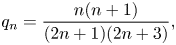 \begin{gather} \displaystyle q_{n} =\frac{n(n+1)}{(2n+1)(2n+3)}, \end{gather}
 \begin{equation}r_{n}=\frac{(n-1)o_{n}}{2n-3},\quad s_{n}=\frac{(n-2)o_{n}}{2n-3}+\frac{(n+1)p_{n}}{2n+1}, \end{equation}
 \begin{equation}t_{n}=\frac{np_{n}}{2n+1}+\frac{(n+3)q_{n}}{2n+5},\quad u_{n}=\frac{(n+2)q_{n}}{2n+5}. \end{equation}


 Open access

