


1 Introduction
Ultra-intense laser systems are employed in a broad range of applications in high-energy-density and relativistic laser–plasma physics. These research fields – enabled by the 2018 Nobel Prize awarded chirped-pulse amplification (CPA) concept[
Reference Strickland and Mourou1] – continuously drive the demand for higher peak intensities to access new regimes of experimental physics, including high-temperature plasma generation, ultra-compact particle acceleration and even strong field quantum electrodynamic phenomena[
Reference Albert, Couprie, Debus, Downer, Faure, Flacco, Gizzi, Grismayer, Huebl, Joshi, Labat, Leemans, Maier, Mangles, Mason, Mathieu, Muggli, Nishiuchi, Osterhoff, Rajeev, Schramm, Schreiber, Thomas, Vay, Vranic and Zeil2]. Recent large-scale ultrafast laser projects target peak powers of the order of 10 PW per pulse to achieve irradiances exceeding 10
 ${}^{23}$
W/cm
${}^{23}$
W/cm
 ${}^2$
at focus (see, e.g., Refs. [Reference Cernaianu, Ghenuche, Rotaru, Tudor, Chalus, Gheorghiu, Popescu, Gugiu, Balascuta, Magureanu, Tataru, Horny, Corobean, Dancus, Alincutei, Asavei, Diaconescu, Dinca, Dreghici, Ghita, Jalba, Leca, Lupu, Nastasa, Negoita, Patrascoiu, Schimbeschi, Stutman, Ticos, Ursescu, Arefiev, Tomassini, Malka, Gales, Tanaka, Ur and Doria3,Reference Radier, Chalus, Charbonneau, Thambirajah, Deschamps, David, Barbe, Etter, Matras, Ricaud, Leroux, Richard, Lureau, Baleanu, Banici, Gradinariu, Caldararu, Capiteanu, Naziru, Diaconescu, Iancu, Dabu, Ursescu, Dancus, Alexandru, Tanaka and Zamfir4]). At such intensities, temporal contrast ratios better than 10
${}^2$
at focus (see, e.g., Refs. [Reference Cernaianu, Ghenuche, Rotaru, Tudor, Chalus, Gheorghiu, Popescu, Gugiu, Balascuta, Magureanu, Tataru, Horny, Corobean, Dancus, Alincutei, Asavei, Diaconescu, Dinca, Dreghici, Ghita, Jalba, Leca, Lupu, Nastasa, Negoita, Patrascoiu, Schimbeschi, Stutman, Ticos, Ursescu, Arefiev, Tomassini, Malka, Gales, Tanaka, Ur and Doria3,Reference Radier, Chalus, Charbonneau, Thambirajah, Deschamps, David, Barbe, Etter, Matras, Ricaud, Leroux, Richard, Lureau, Baleanu, Banici, Gradinariu, Caldararu, Capiteanu, Naziru, Diaconescu, Iancu, Dabu, Ursescu, Dancus, Alexandru, Tanaka and Zamfir4]). At such intensities, temporal contrast ratios better than 10
 ${}^{-12}$
together with absolute knowledge of the exact pulse shape are required on time scales ranging from nanoseconds to tens of picoseconds before the main pulse[
Reference Bagnoud and Wagner5–
Reference Shou, Wu, Pae, Ahn, Kim, Kim, Yoon, Sung, Lee, Gong, Yan, Choi and Nam9] for laser–plasma interactions with solid-state targets. Although various amplification techniques are employed, all systems rely on CPA[
Reference Strickland and Mourou1] to mitigate optical damage and nonlinear effects during amplification and pulse shaping. CPA uses pulse stretchers and compressors to tailor the spectral phase, thereby increasing pulse duration and reducing peak power. These devices typically use diffraction gratings to geometrically disperse the pulse into its spectral components. However, surface imperfections on these optical elements directly affect the spectral phase of the pulse. As peak powers increase, so do the demands on the temporal stretching and beam diameter, making the system more susceptible to spatiotemporal contrast degradation[
Reference Jolly, Gobert and Quéré10,
Reference Bromage, Dorrer and Jungquist11]. While spatiotemporal coupling is often discussed in the context of low-frequency components[
Reference Jolly, Gobert and Quéré10], which primarily affect the shape of the main pulse, contributions at higher temporal frequencies – extending to more than ten times the Fourier-limited pulse duration – are at least equally critical, as they lead to pre-plasma formation in the application[
Reference Bernert, Assenbaum, Bock, Brack, Cowan, Curry, Garten, Gaus, Gauthier, Gebhardt, Göde, Glenzer, Helbig, Kluge, Kraft, Kroll, Obst-Huebl, Püschel, Rehwald, Schlenvoigt, Schoenwaelder, Schramm, Treffert, Vescovi, Ziegler and Zeil12]. Bromage et al. [
Reference Bromage, Dorrer and Jungquist11] theoretically demonstrated that imperfections in stretcher and compressor optics can generate spatiotemporal pedestals with distinct slopes in both the temporal and far-field (k–t) domains. These pedestals have been partially validated experimentally using third-order cross-correlators to probe temporal contrast in the near and far-field[
Reference Lu, Wang, Leng, Guo, Peng, Li, Xu, Xu and Qi13,
Reference Roeder, Zobus, Major and Bagnoud14] or a spatiotemporal cross-correlator on a specific experiment on stretcher–compressor apparatus[
Reference Ma, Yuan, Wang, Wang, Xie, Zhu and Qian15]. However, a full high-resolution single-shot spatiotemporal characterization confirming these slopes experimentally at the output of a TW-class laser system has not been achieved to date. In this work, we demonstrate that spatiotemporal pedestals can be characterized using imaging spectrometry in combination with self-referenced two-dimensional spectral interferometry[
Reference Oksenhendler, Bizouard, Albert, Bock and Schramm16,
Reference Oksenhendler, Bock, Dreyer, Gebhardt, Helbig, Toncian and Schramm17].
${}^{-12}$
together with absolute knowledge of the exact pulse shape are required on time scales ranging from nanoseconds to tens of picoseconds before the main pulse[
Reference Bagnoud and Wagner5–
Reference Shou, Wu, Pae, Ahn, Kim, Kim, Yoon, Sung, Lee, Gong, Yan, Choi and Nam9] for laser–plasma interactions with solid-state targets. Although various amplification techniques are employed, all systems rely on CPA[
Reference Strickland and Mourou1] to mitigate optical damage and nonlinear effects during amplification and pulse shaping. CPA uses pulse stretchers and compressors to tailor the spectral phase, thereby increasing pulse duration and reducing peak power. These devices typically use diffraction gratings to geometrically disperse the pulse into its spectral components. However, surface imperfections on these optical elements directly affect the spectral phase of the pulse. As peak powers increase, so do the demands on the temporal stretching and beam diameter, making the system more susceptible to spatiotemporal contrast degradation[
Reference Jolly, Gobert and Quéré10,
Reference Bromage, Dorrer and Jungquist11]. While spatiotemporal coupling is often discussed in the context of low-frequency components[
Reference Jolly, Gobert and Quéré10], which primarily affect the shape of the main pulse, contributions at higher temporal frequencies – extending to more than ten times the Fourier-limited pulse duration – are at least equally critical, as they lead to pre-plasma formation in the application[
Reference Bernert, Assenbaum, Bock, Brack, Cowan, Curry, Garten, Gaus, Gauthier, Gebhardt, Göde, Glenzer, Helbig, Kluge, Kraft, Kroll, Obst-Huebl, Püschel, Rehwald, Schlenvoigt, Schoenwaelder, Schramm, Treffert, Vescovi, Ziegler and Zeil12]. Bromage et al. [
Reference Bromage, Dorrer and Jungquist11] theoretically demonstrated that imperfections in stretcher and compressor optics can generate spatiotemporal pedestals with distinct slopes in both the temporal and far-field (k–t) domains. These pedestals have been partially validated experimentally using third-order cross-correlators to probe temporal contrast in the near and far-field[
Reference Lu, Wang, Leng, Guo, Peng, Li, Xu, Xu and Qi13,
Reference Roeder, Zobus, Major and Bagnoud14] or a spatiotemporal cross-correlator on a specific experiment on stretcher–compressor apparatus[
Reference Ma, Yuan, Wang, Wang, Xie, Zhu and Qian15]. However, a full high-resolution single-shot spatiotemporal characterization confirming these slopes experimentally at the output of a TW-class laser system has not been achieved to date. In this work, we demonstrate that spatiotemporal pedestals can be characterized using imaging spectrometry in combination with self-referenced two-dimensional spectral interferometry[
Reference Oksenhendler, Bizouard, Albert, Bock and Schramm16,
Reference Oksenhendler, Bock, Dreyer, Gebhardt, Helbig, Toncian and Schramm17].
2 Experimental realization
An enhanced two-dimensional self-referenced spectral interferometry (2D SRSI) setup was implemented at the probe beam port of the CPA1 stage of the Draco laser system[ Reference Oksenhendler, Bock, Dreyer, Gebhardt, Helbig, Toncian and Schramm17– Reference Bock, Herrmann, Püschel, Helbig, Gebhardt, Lötfering, Pausch, Zeil, Ziegler, Irman, Oksenhendler, Kon, Nishuishi, Kiriyama, Kondo, Toncian and Schramm19]. The port provides laser pulses of up to 10 mJ energy, centered around 800 nm, with a pulse duration of 30 fs and a repetition rate of 10 Hz. Here, 2 mJ at the entrance of the 2D SRSI device is used in a beam with 5 mm full-width at half-maximum spatial size.
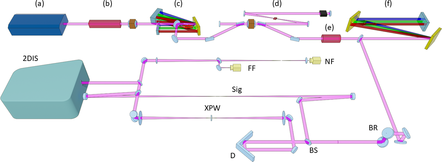
The 2D SRSI interferometer enables spatial–spectral interferometry by combining two pulses at the entrance slit of an imaging spectrometer (Princeton Instruments IsoPlane-320A), equipped with a 12-bit, 16-megapixel complementary metal–oxide–semiconductor (CMOS) camera (ZWO ASI1600MM), as shown in Figure 1. The reference pulse is self-generated from the signal pulse via cross-polarized wave (XPW) generation[ Reference Oksenhendler, Coudreau, Forget, Crozatier, Grabielle, Herzog, Gobert and Kaplan20, Reference Jullien, Canova, Albert, Boschetto, Antonucci, Cha, Rousseau, Chaudet, Chériaux, Etchepare, Kourtev, Minkovski and Saltiel21], which provides a spatially, spectrally and temporally clean reference, while the signal pulse remains undisturbed. Details of the 2D SRSI setup used can be found in Ref. [Reference Oksenhendler, Bock, Dreyer, Gebhardt, Helbig, Toncian and Schramm17], while the study of the SRSI method, its validity domain, algorithm and limitations are described in Ref. [Reference Oksenhendler22].
The oscillator (a) output is first amplified in a booster amplifier (b) and subsequently stretched in a classical Öffner stretcher (c). Further amplification and spectral pulse shaping are performed in a regenerative amplifier (d) and a multipass amplifier (e). The pulses are then compressed in an in-air compressor (f). A periscope (BR) rotates the pulse orientation by 90° to match the horizontal plane of the stretcher and compressor with the vertical slit of the spectrometer. In the 2D SRSI, a beamsplitter (BS) separates the light: the transmitted part is used to generate the reference (XPW) and the corresponding delay (D), while the reflected part is directed along the signal path (Sig) to the entrance slit of the imaging spectrometer (2DIS), where it is re-combined with the reference.

To ensure consistent spatial orientation throughout the system, the pulse stretcher is first aligned to match the spatial dispersion plane of the air-based compressor. Subsequently, both the stretcher and compressor are jointly matched to the vertical slit orientation of the imaging spectrometer. For this purpose, a periscope is positioned behind the compressor to rotate the beam such that the horizontal dispersion plane of the compressor and the stretcher aligns with the vertical spatial detection axis of the spectrometer.
The measured interferogram can be expressed as follows:
 $$\begin{align}\tilde{S}\left(x,\omega \right)=\tilde{S_0}\left(x,\omega \right)+\tilde{f}\left(x,\omega \right){e}^{i\left(\omega \tau +{k}_xx\right)}+{\tilde{f}}^{\ast}\left(x,\omega \right){e}^{-i\left(\omega \tau +{k}_xx\right)},\end{align}$$
where the DC term is given by the following:
 $$\begin{align}\tilde{S_0}\left(x,\omega \right)={\left|{\tilde{E}}_{\mathrm{Ref}}\left(x,\omega \right)\right|}^2+{\left|{\tilde{E}}_{\mathrm{in}}\left(x,\omega \right)\right|}^2,\end{align}$$
that is, the sum of the spectra of the XPW-filtered reference pulse
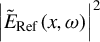 ${\left|{\tilde{E}}_{\mathrm{Ref}}\left(x,\omega \right)\right|}^2$
and the signal input pulse to be measured
${\left|{\tilde{E}}_{\mathrm{Ref}}\left(x,\omega \right)\right|}^2$
and the signal input pulse to be measured
 ${\left|{\tilde{E}}_{\mathrm{in}}\left(x,\omega \right)\right|}^2$
. The AC term is given by the following:
${\left|{\tilde{E}}_{\mathrm{in}}\left(x,\omega \right)\right|}^2$
. The AC term is given by the following:
 $$\begin{align}\tilde{f}\left(x,\omega \right)={\tilde{E}}_{\mathrm{Ref}}^{\ast}\left(x,\omega \right)\kern0.1em {\tilde{E}}_{\mathrm{in}}\left(x,\omega \right),\end{align}$$
that is, the interference of the two pulses. This formulation follows the principles of classical Fourier transform spectral interferometry[
Reference Oksenhendler, Coudreau, Forget, Crozatier, Grabielle, Herzog, Gobert and Kaplan20], with the distinction that the separation of AC and DC terms in the Fourier domain appears along the temporal axis and the spatial frequency axis in the temporal far-field k
 ${}_x$
–t domain. This is illustrated in Figure 2 by the intensity term DC (
${}_x$
–t domain. This is illustrated in Figure 2 by the intensity term DC (
 $\tilde{S_0}\left(x,\omega \right)$
) and AC cross-correlation field term (
$\tilde{S_0}\left(x,\omega \right)$
) and AC cross-correlation field term (
 $\tilde{f}\left(x,\omega \right)$
).
$\tilde{f}\left(x,\omega \right)$
).
Temporal far-field intensity in the logarithmic scale of the interferogram. The spatio-spectral interferogram is shown in the inset.
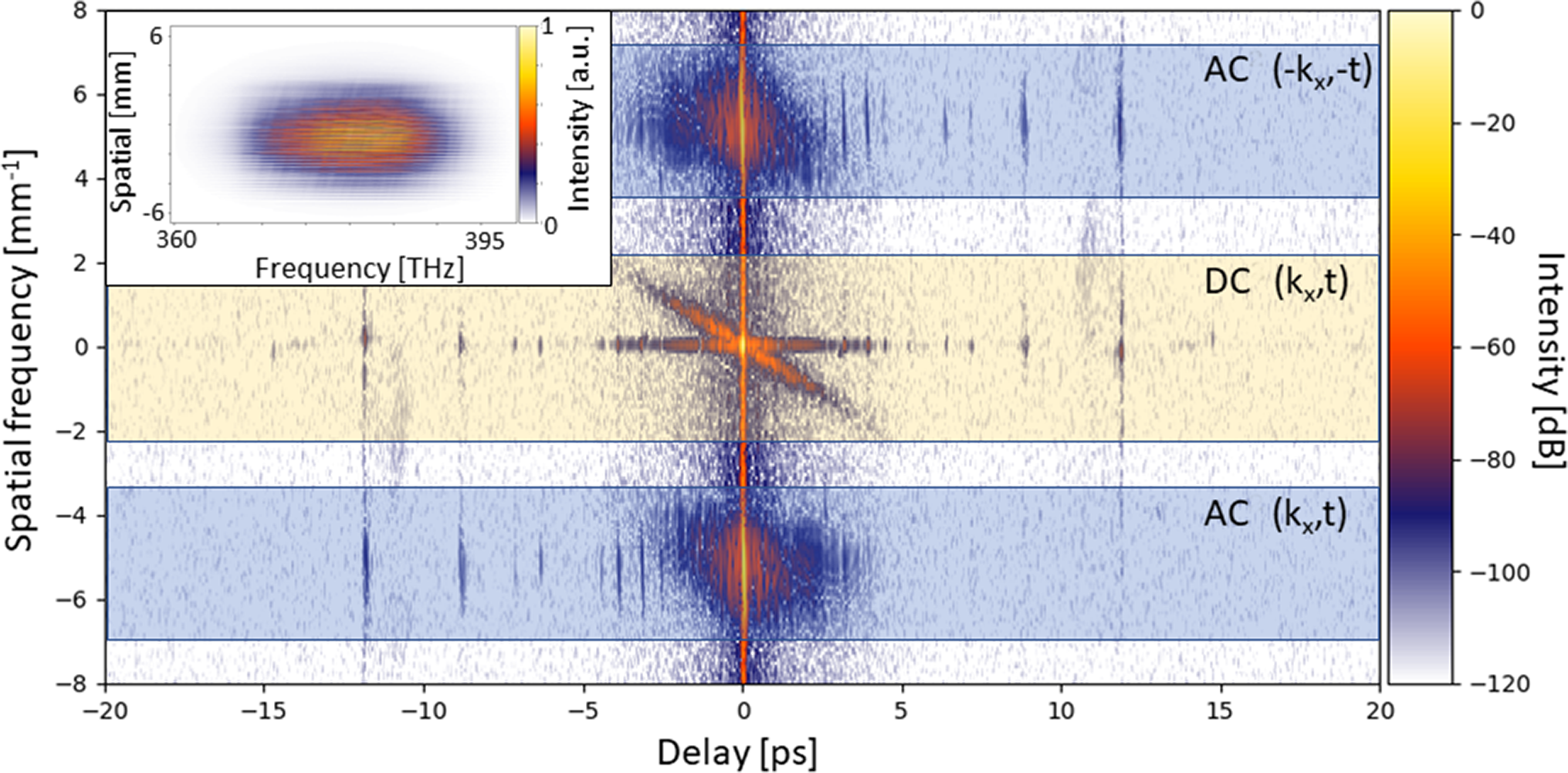
The central term DC is centrosymmetric in the k
 ${}_x$
–t domain. Since this symmetry is centered around the zero-frequency point, it already reveals the contribution of the pedestal along a diagonal line. Indeed, as theoretically predicted[
Reference Bromage, Dorrer and Jungquist11], in the time-domain far-field, the pedestals arising from near-field contributions follow diagonal structures. In contrast, the contribution from the convex mirror of the employed Öffner stretcher, which is located in the far-field, manifests as a pedestal aligned along the temporal axis. The corresponding far-field intensity in the time domain can be expressed in the following form[
Reference Bromage, Dorrer and Jungquist11]:
${}_x$
–t domain. Since this symmetry is centered around the zero-frequency point, it already reveals the contribution of the pedestal along a diagonal line. Indeed, as theoretically predicted[
Reference Bromage, Dorrer and Jungquist11], in the time-domain far-field, the pedestals arising from near-field contributions follow diagonal structures. In contrast, the contribution from the convex mirror of the employed Öffner stretcher, which is located in the far-field, manifests as a pedestal aligned along the temporal axis. The corresponding far-field intensity in the time domain can be expressed in the following form[
Reference Bromage, Dorrer and Jungquist11]:
 $$\begin{align} \left\langle I\left({k}_x,{k}_y,t\right)\right\rangle &={I}_0\left({k}_x,{k}_y,t\right)\nonumber\\&\quad + {\int}_{{\kern-6pt}-\infty}^{\infty}\mathrm{d}{t}^{\prime}\kern0.1em {I}_0\left({k}_x,{k}_y,{t}^{\prime}\right)\kern0.1em {\mathrm{PSD}}_{\mathrm{cvx}}\left(t-{t}^{\prime}\right)\nonumber\\&\quad + \sum \limits_n{\int}_{{\kern-6pt}-\infty}^{\infty }{\int}_{{\kern-6pt}-\infty}^{\infty}\mathrm{d}u\kern0.1em \mathrm{d}v\kern0.1em {I}_0\left(u,v,t+{\gamma}_n{k}_x-{\gamma}_nu\right)\nonumber\\&\quad \times {\mathrm{PSD}}_n\left({k}_x-u,{k}_y-v\right),\end{align}$$
where I
 ${}_0$
denotes the far-field intensity of the pulse in the absence of spatiotemporal contributions, PSD
${}_0$
denotes the far-field intensity of the pulse in the absence of spatiotemporal contributions, PSD
 ${}_{\mathrm{cvx}}$
is the power spectral density of the phase screen equivalent to the surface of the convex mirror, and PSD
${}_{\mathrm{cvx}}$
is the power spectral density of the phase screen equivalent to the surface of the convex mirror, and PSD
 ${}_n$
represents the power spectral densities of the phase screens corresponding to near-field optics, such as the concave mirror, diffraction gratings or folding mirrors. The parameters
${}_n$
represents the power spectral densities of the phase screens corresponding to near-field optics, such as the concave mirror, diffraction gratings or folding mirrors. The parameters
 ${\gamma}_n$
are the spatio-spectral coupling coefficients (in mm/THz), which determine the central position of the beam on a given optical element as a function of the optical frequency
${\gamma}_n$
are the spatio-spectral coupling coefficients (in mm/THz), which determine the central position of the beam on a given optical element as a function of the optical frequency
 $\omega$
by
$\omega$
by
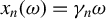 $x_n(\omega) = \gamma_n \omega$
. In our configuration, the main contributions originate from two key optical components: the second and third gratings (pass), and the roof mirror of the air compressor and the convex mirror of the Öffner stretcher. The contribution from the second and third gratings (pass) and the roof mirror is expected to appear along a diagonal in the k
$x_n(\omega) = \gamma_n \omega$
. In our configuration, the main contributions originate from two key optical components: the second and third gratings (pass), and the roof mirror of the air compressor and the convex mirror of the Öffner stretcher. The contribution from the second and third gratings (pass) and the roof mirror is expected to appear along a diagonal in the k
 ${}_x$
–t domain, with a slope of
${}_x$
–t domain, with a slope of
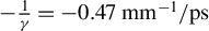 ${-\frac{1}{\gamma }=-0.47\;{\mathrm{mm}}^{-1}/\mathrm{ps}}$
, resulting from the dispersion and setting of the compressor. In contrast, the contribution from the convex mirror, being a far-field optical element, is aligned along the temporal axis. Other contributions are expected with different slopes but at a much lower level due to the surface quality of their original optical component[
Reference Bromage, Dorrer and Jungquist11,
Reference Roeder, Zobus, Major and Bagnoud14,
Reference Ma, Yuan, Wang, Wang, Xie, Zhu and Qian15].
${-\frac{1}{\gamma }=-0.47\;{\mathrm{mm}}^{-1}/\mathrm{ps}}$
, resulting from the dispersion and setting of the compressor. In contrast, the contribution from the convex mirror, being a far-field optical element, is aligned along the temporal axis. Other contributions are expected with different slopes but at a much lower level due to the surface quality of their original optical component[
Reference Bromage, Dorrer and Jungquist11,
Reference Roeder, Zobus, Major and Bagnoud14,
Reference Ma, Yuan, Wang, Wang, Xie, Zhu and Qian15].
3 Results
In the first place the expected characteristics in the k
 ${}_x$
–t space can be seen in the DC cross-correlation term. When using only one beam path (signal or reference) the DC
${}_x$
–t space can be seen in the DC cross-correlation term. When using only one beam path (signal or reference) the DC
 ${}^2$
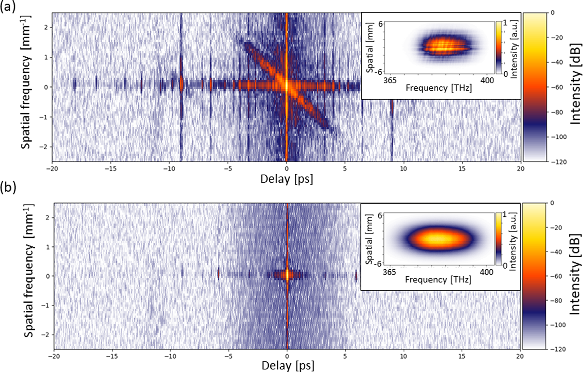
term represents an intensity autocorrelation in the far-field. Figure 3 shows the results for the signal and XPW reference individually. The signal measurement clearly reveals the effects of optical imperfections introduced by the stretcher and compressor. In contrast, in the measurement of the reference the spatial-temporal structures are absent, due to the pulse cleaning of the XPW effect. Nevertheless, due to the autocorrelation nature of the DC, phase information and potential asymmetric temporal shape are lost. The slope of the spatial-temporal tilted contribution is –0.47 mm
${}^2$
term represents an intensity autocorrelation in the far-field. Figure 3 shows the results for the signal and XPW reference individually. The signal measurement clearly reveals the effects of optical imperfections introduced by the stretcher and compressor. In contrast, in the measurement of the reference the spatial-temporal structures are absent, due to the pulse cleaning of the XPW effect. Nevertheless, due to the autocorrelation nature of the DC, phase information and potential asymmetric temporal shape are lost. The slope of the spatial-temporal tilted contribution is –0.47 mm
 ${}^{-1}$
/ps, as expected. To reveal the phase information, as well as the temporal shape of the laser pulse, the signal and reference pulses have to be spatial-spectrally interfered in the 2D SRSI. Thus, not only are the DC terms present in the k
${}^{-1}$
/ps, as expected. To reveal the phase information, as well as the temporal shape of the laser pulse, the signal and reference pulses have to be spatial-spectrally interfered in the 2D SRSI. Thus, not only are the DC terms present in the k
 ${}_x$
–t space, but also the AC term as cross-correlation of the signal and reference. The same contribution as in the DC term appears on the AC term, but it is blurred by a slight defocusing between the two arms of the interferometer (Figure 2). After subtracting this unintended defocusing contribution in the data post-treatment, the two signals AC
${}_x$
–t space, but also the AC term as cross-correlation of the signal and reference. The same contribution as in the DC term appears on the AC term, but it is blurred by a slight defocusing between the two arms of the interferometer (Figure 2). After subtracting this unintended defocusing contribution in the data post-treatment, the two signals AC
 ${}^2$
and DC show the pedestal on the same diagonal slope, as shown in Figure 4. The intensity profiles extracted from the DC term (Figure 4(a)) are symmetrical in time because they correspond to the sum of the autocorrelations of signal and reference, whereas for the AC
${}^2$
and DC show the pedestal on the same diagonal slope, as shown in Figure 4. The intensity profiles extracted from the DC term (Figure 4(a)) are symmetrical in time because they correspond to the sum of the autocorrelations of signal and reference, whereas for the AC
 ${}^2$
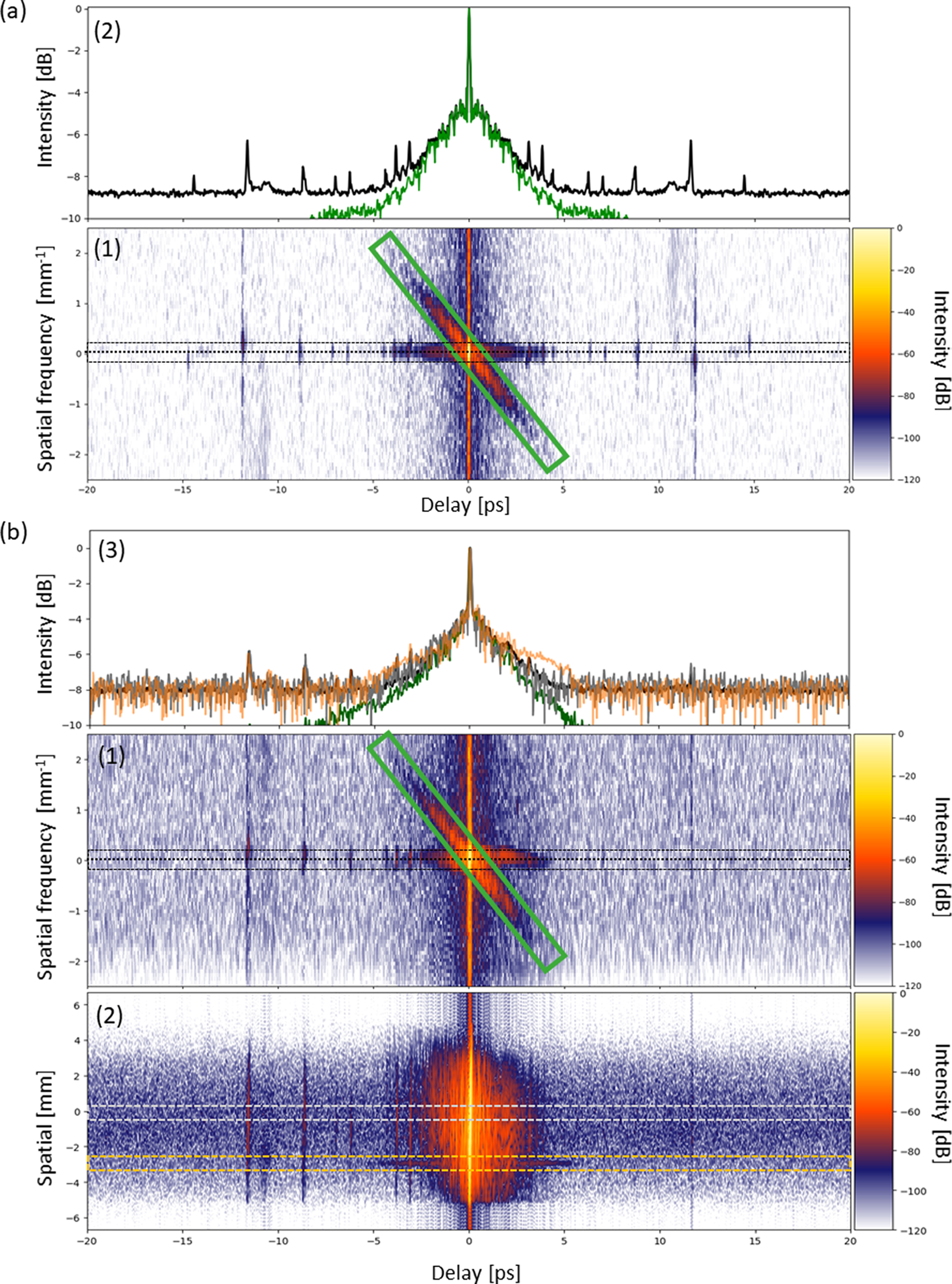
term (Figure 4(b)) the cross-correlation between the signal and references reveals the temporal (asymmetric) shape. The slope is identical for both terms and corresponds to the compressor parameters. In our case, the two contributions in the far-field are almost equivalent, as shown by the black and green curves in Figure 4(b) panel (3).
${}^2$
term (Figure 4(b)) the cross-correlation between the signal and references reveals the temporal (asymmetric) shape. The slope is identical for both terms and corresponds to the compressor parameters. In our case, the two contributions in the far-field are almost equivalent, as shown by the black and green curves in Figure 4(b) panel (3).
Temporal far-field intensity in logarithmic scale of the spectrogram, the spatio-spectral intensity of which is shown in the inset (a) for the signal and (b) for the XPW cleaned reference pulse.

(a) (1) Temporal/far-field intensity in log scale of the interferogram for the DC term and (2) the intensity profiles along the green box and black dotted line. (b) (1) Temporal/far-field intensity in log scale of the interferogram for the AC
 ${}^2$
term, (2) its temporal/near-field intensity and (3) the intensity profiles along the green box and black dotted line for the far-field domain, and grey and orange for the central position and a lateral position showing a defect.
${}^2$
term, (2) its temporal/near-field intensity and (3) the intensity profiles along the green box and black dotted line for the far-field domain, and grey and orange for the central position and a lateral position showing a defect.
The inclined pedestal is generally not detected by third-order cross-correlators measuring in the far-field[ Reference Schanz, Wagner, Roth and Bagnoud23]. This type of device then only measures the pedestal along the temporal dimension, caused by the convex mirror in the stretcher.
Other third-order cross-correlators[
Reference Bock, Oksenhendler, Püschel, Gebhardt, Helbig, Pausch, Ziegler, Bernert, Zeil, Irman, Toncian, Kiriyama, Nishiuchi, Kon and Schramm18,
Reference Luan, Hutchinson, Smith and Zhou24] measure in the near-field instead, where the two contributions are almost indistinguishable because the inclination is small compared with the size of the beam; both contributions are overlapping. The spatiotemporal cross-correlation measurement[
Reference Ma, Yuan, Wang, Wang, Xie, Zhu and Qian15] should be able to measure it, but it suffers from low temporal resolution (0.5 ps) and spatial frequency in the far-field (
 $>$
0.2 mrad) despite the need to scan the spatial dimension. In addition, it has not yet been used to measure the spatiotemporal pedestal at the output of a TW-class laser beam. Here, we can derive a similar measurement as a near-field cross-correlator would provide by Fourier-transforming the spatial frequency axis of the AC
$>$
0.2 mrad) despite the need to scan the spatial dimension. In addition, it has not yet been used to measure the spatiotemporal pedestal at the output of a TW-class laser beam. Here, we can derive a similar measurement as a near-field cross-correlator would provide by Fourier-transforming the spatial frequency axis of the AC
 ${}^2$
term back to the spatial dimension. In our measurement by the 2D SRSI the spatial resolution reveals a local deterioration, as can be seen when comparing the temporal intensity profile at the central part of the near-field along the grey dotted box in Figure 4(b) panel (2) in comparison to the profile along the orange region on the side of the near-field profile in Figure 4(b) panel (3). A typical near-field cross-correlator detects the total average of such a near-field profile.
${}^2$
term back to the spatial dimension. In our measurement by the 2D SRSI the spatial resolution reveals a local deterioration, as can be seen when comparing the temporal intensity profile at the central part of the near-field along the grey dotted box in Figure 4(b) panel (2) in comparison to the profile along the orange region on the side of the near-field profile in Figure 4(b) panel (3). A typical near-field cross-correlator detects the total average of such a near-field profile.
Since, in our case, the dominant contribution comes from the convex mirror, the temporal intensity profiles are almost identical in the near- and far-field. Nevertheless, as the contribution of the compressor is fairly close, improving the surface quality of this mirror should only significantly increase the contrast in the far-field. Indeed, few improvements are expected in the near-field, which is also limited by the contributions of other optics, notably the second, third gratings (pass) and roof mirror of the compressor.
4 Conclusion
In conclusion, the presented measurement results demonstrate the potential of 2D SRSI for capturing high-dynamic-range spatiotemporal features. Even a simpler measurement using only an imaging spectrometer provides access to the spatiotemporal intensity autocorrelation of the pedestal generated by the compressor grating. Both techniques operate in single-shot mode and can be implemented on large-scale ultrafast laser systems, where accurate characterization of such pedestals is essential. Since 2D SRSI measures the full electric field, a single acquisition allows for simultaneous evaluation of near-field and far-field contributions with high resolution and wide coverage in both spatial and temporal domains. This enables the identification of previously undetectable spatiotemporal distortions and facilitates the optimization of laser system performance. It is important to emphasize that the observed asymmetry in the far-field profile indicates that particular care must be taken in aligning the beam on the experimental target – especially in solid-state experiments. For spatiotemporally inclined pedestals, the incidence angle of the light on the target varies in time. As a result, the effective delay depends on the target angle, potentially leading to asymmetries in the pulse contrast. In high-contrast experiments, two opposite angles of incidence may thus produce significantly different temporal contrast profiles.


 Open access