


1. Introduction
The study of pattern formation in fluid dynamics has garnered significant interest over several decades. One such example is the emergence of laminar–turbulent patterns in the route-to-transition, where laminar and turbulent regions coexist in a self-organized, spatially intermittent manner. Pioneering research by Coles (Reference Coles1965) and Van Atta (Reference Van Atta1966) studied pattern formation in Taylor–Couette flow, revealing the formation of alternating turbulent and laminar spirals. This study paved the way for investigating laminar–turbulent pattern formation in other shear-driven systems, including plane Couette flow (PCF).
The experiments of Prigent et al. (Reference Prigent, Grégoire, Chaté, Dauchot and van Saarloos2002, Reference Prigent, Grégoire, Chaté and Dauchot2003) laid the foundation for exploring laminar–turbulent pattern formation in PCF. When PCF transitions from turbulent to laminar flow, it exhibits alternating laminar–turbulent bands with large wavelengths and an oblique orientation to the streamwise direction. Owing to the pattern’s large wavelength, its existence is limited to experiments and direct numerical simulation (DNS) performed in large domains. Barkley & Tuckerman (Reference Barkley and Tuckerman2005) overcame the need for a large-aspect ratio system by using an inclined domain perpendicular to the pattern. This was also the first DNS study to capture laminar–turbulent bands in PCF. In their subsequent study (Barkley & Tuckerman Reference Barkley and Tuckerman2007), they investigated the large-scale components of the flow and highlighted that they run parallel to the laminar–turbulent boundaries. Later, Manneville & Rolland (Reference Manneville and Rolland2011) performed under-resolved simulations to capture oblique bands in a large-aspect-ratio system, successfully preserving their main features; however, this approach led to a downward shift in the transitional Reynolds number range compared with that observed in experiments. All of the aforementioned studies examined the formation of laminar–turbulent bands during the reverse transition, where the flow is first taken to a fully turbulent state and then the Reynolds number is reduced to reach transition. In contrast, Duguet, Schlatter & Henningson (Reference Duguet, Schlatter and Henningson2010) investigated pattern formation in PCF as it transitions from laminar to turbulent flow when subjected to finite-amplitude perturbations. However, this methodology is highly dependent on the specific characteristics of the perturbations. A subsequent study by Duguet & Schlatter (Reference Duguet and Schlatter2013) highlighted the role of large-scale flow in the evolution of a turbulent spot into an oblique turbulent band.
Most studies on the transition to turbulence in PCF have dealt with smooth surfaces. It is natural to question how surface roughness influences pattern formation. Ishida et al. (Reference Ishida, Brethouwer, Duguet and Tsukahara2017) studied the robustness of the laminar–turbulent pattern under the influence of wall roughness using a parametric roughness model developed by Busse & Sandham (Reference Busse and Sandham2012). They explored the impact of roughness by varying its shape, employing rectangular and Gaussian shape functions, and examined a range of roughness heights from $0.05h$
to
$0.05h$
to $0.5h$
(where
$0.5h$
(where $h$
is the half-channel height). Their computations revealed that the laminar–turbulent pattern remains robust for roughness heights up to
$h$
is the half-channel height). Their computations revealed that the laminar–turbulent pattern remains robust for roughness heights up to $0.3h$
. For heights exceeding
$0.3h$
. For heights exceeding $0.3h$
, however, the pattern loses its oblique structure, giving rise to a new pattern that they termed transverse turbulent bands. A subsequent study by Tsukahara et al. (Reference Tsukahara, Tomioka, Ishida, Duguet and Brethouwer2018) explored the unique characteristics of transverse turbulent bands. They found that the transverse turbulent bands can be sustained even when the average turbulent fraction drops to 10
$0.3h$
, however, the pattern loses its oblique structure, giving rise to a new pattern that they termed transverse turbulent bands. A subsequent study by Tsukahara et al. (Reference Tsukahara, Tomioka, Ishida, Duguet and Brethouwer2018) explored the unique characteristics of transverse turbulent bands. They found that the transverse turbulent bands can be sustained even when the average turbulent fraction drops to 10 $\%$
. Another notable observation was the absence of a significant large-scale spanwise component associated with the transverse bands. This observation also highlights the crucial role of large-scale spanwise flow in forming oblique bands. All of the roughness studies we have discussed so far have employed parametric models to investigate roughness effects. These models are limited in their ability to capture small-scale turbulent phenomena, such as vortex shedding behind individual roughness elements (Busse & Sandham Reference Busse and Sandham2012). Therefore, our recent study (Gokul & Narasimhamurthy Reference Gokul and Narasimhamurthy2024) utilized real roughness elements to investigate the impact of roughness on pattern formation. Two-dimensional square ribs with a height of
$\%$
. Another notable observation was the absence of a significant large-scale spanwise component associated with the transverse bands. This observation also highlights the crucial role of large-scale spanwise flow in forming oblique bands. All of the roughness studies we have discussed so far have employed parametric models to investigate roughness effects. These models are limited in their ability to capture small-scale turbulent phenomena, such as vortex shedding behind individual roughness elements (Busse & Sandham Reference Busse and Sandham2012). Therefore, our recent study (Gokul & Narasimhamurthy Reference Gokul and Narasimhamurthy2024) utilized real roughness elements to investigate the impact of roughness on pattern formation. Two-dimensional square ribs with a height of $k=0.2h$
were used, with two pitch separations examined:
$k=0.2h$
were used, with two pitch separations examined: $\lambda = 2k$
and
$\lambda = 2k$
and $\lambda =10k$
, which belong to the d-type and k-type roughness classes, respectively. (The terms d-type and k-type indicate the relevant length scales: the pipe diameter (
$\lambda =10k$
, which belong to the d-type and k-type roughness classes, respectively. (The terms d-type and k-type indicate the relevant length scales: the pipe diameter ( $d$
) or boundary layer thickness (
$d$
) or boundary layer thickness ( $\delta$
) for d-type roughness, and the roughness height (
$\delta$
) for d-type roughness, and the roughness height ( $k$
) for k-type roughness (Perry, Schofield & Joubert Reference Perry, Schofield and Joubert1969). We observed that the shift in the transitional range induced by the roughness elements depends on their ability to provide an additional mechanism for streamwise vorticity regeneration. Consequently, we found that the k-type roughness, due to its ability to shed vortices above the rib crests, can regenerate streamwise vorticity and thereby sustain a laminar–turbulent pattern at significantly lower Reynolds numbers than the d-type roughness and the smooth PCF.
$k$
) for k-type roughness (Perry, Schofield & Joubert Reference Perry, Schofield and Joubert1969). We observed that the shift in the transitional range induced by the roughness elements depends on their ability to provide an additional mechanism for streamwise vorticity regeneration. Consequently, we found that the k-type roughness, due to its ability to shed vortices above the rib crests, can regenerate streamwise vorticity and thereby sustain a laminar–turbulent pattern at significantly lower Reynolds numbers than the d-type roughness and the smooth PCF.
The current study aims to explore the laminar–turbulent pattern formation in PCF with three-dimensional (3-D) roughness, which is characterized by alternating rough and smooth zones. To the best of our knowledge, this is the first such attempt to disseminate transition physics from real 3-D roughness in PCF. We report both instantaneous and mean flow characteristics of 3-D roughness in the transitional regime, with frequent comparisons with those of two-dimensional (2-D) roughness to highlight the fundamental differences. Particular attention is given to spatiotemporal dynamics, evolution of coherent structures and dynamics of large-scale motion in this DNS study.
2. Methodology
The flow configuration is shown in figure 1(a). The coordinate axes $x$
,
$x$
, $y$
and
$y$
and $z$
represent the streamwise, spanwise and wall-normal directions, respectively. Fluid flow occurs between two infinitely long parallel plates separated by a distance of
$z$
represent the streamwise, spanwise and wall-normal directions, respectively. Fluid flow occurs between two infinitely long parallel plates separated by a distance of $2h$
. The lower plate is stationary, and the upper plate moves with a constant velocity
$2h$
. The lower plate is stationary, and the upper plate moves with a constant velocity $U_{w}$
in the
$U_{w}$
in the $x$
-direction, which drives the flow. The Reynolds number (
$x$
-direction, which drives the flow. The Reynolds number ( $\textit{Re} = {U_{w}h}/{2\nu }$
) is based on the half-channel height (
$\textit{Re} = {U_{w}h}/{2\nu }$
) is based on the half-channel height ( $h$
) and half the velocity of top plate (
$h$
) and half the velocity of top plate ( ${U_{w}}/{2}$
). The roughness elements are introduced only on the stationary wall, whereas the moving wall is smooth, resulting in an asymmetric system. Compared with Couette flow set-ups with two rough walls, such asymmetric systems are easy to configure in experiments (Ishida et al. Reference Ishida, Brethouwer, Duguet and Tsukahara2017). The roughness elements used in our study are ribs of height
${U_{w}}/{2}$
). The roughness elements are introduced only on the stationary wall, whereas the moving wall is smooth, resulting in an asymmetric system. Compared with Couette flow set-ups with two rough walls, such asymmetric systems are easy to configure in experiments (Ishida et al. Reference Ishida, Brethouwer, Duguet and Tsukahara2017). The roughness elements used in our study are ribs of height $k=0.2h$
with a square cross-section (
$k=0.2h$
with a square cross-section ( $k=w$
, where
$k=w$
, where $w$
is the width of the ribs). In viscous units, i.e.
$w$
is the width of the ribs). In viscous units, i.e. $k^{+}=ku_{\tau }/\nu$
, the current roughness height varies between 4.69–6.40 in the Re range 325–400, which clearly falls within a buffer layer of a turbulent boundary layer. According to Jiménez (Reference Jiménez2004), if
$k^{+}=ku_{\tau }/\nu$
, the current roughness height varies between 4.69–6.40 in the Re range 325–400, which clearly falls within a buffer layer of a turbulent boundary layer. According to Jiménez (Reference Jiménez2004), if $k^{+}$
lies within a linear sublayer, then it should be considered hydrodynamically smooth. Thereby, reducing the
$k^{+}$
lies within a linear sublayer, then it should be considered hydrodynamically smooth. Thereby, reducing the $k$
value is not an option, and increasing it further makes it bluff body, not roughness. The streamwise pitch separation is
$k$
value is not an option, and increasing it further makes it bluff body, not roughness. The streamwise pitch separation is $\lambda = 10k$
, resulting in wide cavities between the ribs and, therefore, falls into the category of k-type roughness (Jiménez Reference Jiménez2004). The streamwise pitch separation is sufficiently larger than the
$\lambda = 10k$
, resulting in wide cavities between the ribs and, therefore, falls into the category of k-type roughness (Jiménez Reference Jiménez2004). The streamwise pitch separation is sufficiently larger than the $\lambda =4{-}5k$
range, where the d-type to k-type transition occurs, thus avoiding any d-type characteristics. We have considered two roughness configurations: one with 2-D k-type roughness (figure 1
b), where the ribs extend throughout the width of the domain, and the other with 3-D k-type roughness (figure 1
c), where the roughness length and spanwise pitch separation are the same, i.e.
$\lambda =4{-}5k$
range, where the d-type to k-type transition occurs, thus avoiding any d-type characteristics. We have considered two roughness configurations: one with 2-D k-type roughness (figure 1
b), where the ribs extend throughout the width of the domain, and the other with 3-D k-type roughness (figure 1
c), where the roughness length and spanwise pitch separation are the same, i.e. $\delta =85k$
. The transition to turbulence in the 2-D k-type roughness was discussed in our previous study (Gokul & Narasimhamurthy Reference Gokul and Narasimhamurthy2024). The main focus of this study is on the characteristics of 3-D k-type roughness in the transitional regime and how it differs from that of its 2-D counterpart.
$\delta =85k$
. The transition to turbulence in the 2-D k-type roughness was discussed in our previous study (Gokul & Narasimhamurthy Reference Gokul and Narasimhamurthy2024). The main focus of this study is on the characteristics of 3-D k-type roughness in the transitional regime and how it differs from that of its 2-D counterpart.
(a) Schematic of rough Couette flow, (b) 2-D k-type roughness and (c) 3-D k-type roughness, both mounted on the stationary wall. In figure 1(a), I and II denote the positions of the midcavity and midrib, respectively.

The equations that govern the isothermal incompressible flow of a Newtonian fluid are given by
 \begin{equation} \dfrac {\partial u_{i}}{\partial t}+\dfrac {\partial u_{i}u_{j}}{\partial x_{j}}=\dfrac {1}{Re}\dfrac {\partial ^{2} u_{i}}{\partial x_{j}^{2}}-\dfrac {\partial p}{\partial x_{i}}, \end{equation}
 \begin{equation} \dfrac {\partial u_{i}}{\partial x_{i}}=0. \end{equation}
An in-house parallel finite volume solver, MGLET (Manhart Reference Manhart2004), is used to solve these governing equations. The solver employs a staggered Cartesian grid, where the pressure and velocity are computed at the cell centres and faces, respectively. The spatial discretization of the convection and diffusion terms is performed using a central difference scheme. The second-order Adam–Bashforth method, which employs a linear interpolation technique, is utilized for time advancement. The pressure Poisson equation is solved using a multigrid algorithm. The simulations were carried out in a computational box of size $L_{x} \times L_{y} \times L_{z}=136h \times 68h \times 2h$
, capable of accommodating one wavelength of laminar–turbulent bands. The grid size for the 2-D and 3-D k-type roughness configurations is set to
$L_{x} \times L_{y} \times L_{z}=136h \times 68h \times 2h$
, capable of accommodating one wavelength of laminar–turbulent bands. The grid size for the 2-D and 3-D k-type roughness configurations is set to $N_{x} \times N_{y} \times N_{z}=4080 \times 288 \times 108$
. The grid spacing is uniform in the
$N_{x} \times N_{y} \times N_{z}=4080 \times 288 \times 108$
. The grid spacing is uniform in the $x$
and
$x$
and $y$
directions, while in the
$y$
directions, while in the $z$
-direction, it is non-uniform, with a minimum near the walls and a maximum at the channel centre. The meshing is executed such that the faces of the ribs align with the cell faces, with six cells across each rib in the
$z$
-direction, it is non-uniform, with a minimum near the walls and a maximum at the channel centre. The meshing is executed such that the faces of the ribs align with the cell faces, with six cells across each rib in the $x$
-direction, 72 cells along each rib in the
$x$
-direction, 72 cells along each rib in the $y$
-direction, and 20 cells within each rib in the
$y$
-direction, and 20 cells within each rib in the $z$
-direction; ensuring the accurate capture of the flow near each rib. The transition to turbulence in the smooth PCF is also simulated to facilitate comparison with the rough cases. The simulations for the smooth PCF are conducted using the same computational domain as the rough PCF, but the grid size is reduced because of the absence of ribs. Table 1 provides a detailed description of all simulations carried out in this study, including the Reynolds number range, domain size, grid size and grid resolution in the
$z$
-direction; ensuring the accurate capture of the flow near each rib. The transition to turbulence in the smooth PCF is also simulated to facilitate comparison with the rough cases. The simulations for the smooth PCF are conducted using the same computational domain as the rough PCF, but the grid size is reduced because of the absence of ribs. Table 1 provides a detailed description of all simulations carried out in this study, including the Reynolds number range, domain size, grid size and grid resolution in the $x$
-,
$x$
-, $y$
- and
$y$
- and $z$
-directions. Grötzbach (Reference Grötzbach1983) provided a criterion for selecting the appropriate grid resolutions for a DNS, given by
$z$
-directions. Grötzbach (Reference Grötzbach1983) provided a criterion for selecting the appropriate grid resolutions for a DNS, given by $ { ( \Delta x \Delta y \Delta z )^{(1/3)}}/{\pi \eta }\leqslant 1$
. The grids utilized in this study meet the Grötzbach criterion, ensuring that they are fine enough to capture the Kolmogorov length scale
$ { ( \Delta x \Delta y \Delta z )^{(1/3)}}/{\pi \eta }\leqslant 1$
. The grids utilized in this study meet the Grötzbach criterion, ensuring that they are fine enough to capture the Kolmogorov length scale $\eta$
(figure 2). The Kolmogorov length scale,
$\eta$
(figure 2). The Kolmogorov length scale, $\eta$
, characterizes the smallest scales of turbulence and is expressed as
$\eta$
, characterizes the smallest scales of turbulence and is expressed as $\eta = ( {\nu ^{3}}/{\epsilon } )^{(1/4)}$
, where
$\eta = ( {\nu ^{3}}/{\epsilon } )^{(1/4)}$
, where $\nu$
represents the kinematic viscosity of the fluid, and
$\nu$
represents the kinematic viscosity of the fluid, and $\epsilon$
denotes the dissipation rate of turbulent kinetic energy. The time step size is set to
$\epsilon$
denotes the dissipation rate of turbulent kinetic energy. The time step size is set to $\Delta t =0.01$
, ensuring that it is smaller than the Kolmogorov time scale and satisfies the Courant–Friedrichs–Lewy stability condition. The periodic boundary condition is imposed in the
$\Delta t =0.01$
, ensuring that it is smaller than the Kolmogorov time scale and satisfies the Courant–Friedrichs–Lewy stability condition. The periodic boundary condition is imposed in the $x$
- and
$x$
- and $y$
-directions, while the no-slip boundary condition is implemented on the walls and the rib surfaces. The accuracy of the computations was validated by comparison with existing studies on turbulent Couette flows (Gokul & Narasimhamurthy Reference Gokul and Narasimhamurthy2024). For more numerical details, please refer to this article.
$y$
-directions, while the no-slip boundary condition is implemented on the walls and the rib surfaces. The accuracy of the computations was validated by comparison with existing studies on turbulent Couette flows (Gokul & Narasimhamurthy Reference Gokul and Narasimhamurthy2024). For more numerical details, please refer to this article.
Description of the simulations conducted in this study. The grid resolutions are determined according to the friction Reynolds number ( $\textit{Re}_{\tau }=u_{\tau }h/\nu$
, where
$\textit{Re}_{\tau }=u_{\tau }h/\nu$
, where $u_{\tau }$
is the friction velocity) of the respective case.
$u_{\tau }$
is the friction velocity) of the respective case.

Contour plot of $\varDelta /\pi \eta$
in an
$\varDelta /\pi \eta$
in an $x{-}z$
plane for (a) 3-D k-type roughness (
$x{-}z$
plane for (a) 3-D k-type roughness ( $y/h = 17$
) and (b) 2-D k-type roughness (
$y/h = 17$
) and (b) 2-D k-type roughness ( $y/h = 34$
).
$y/h = 34$
). $\textit{Re}=400$
in both cases.
$\textit{Re}=400$
in both cases.

3. Results and discussion
The reverse transition is achieved using a computational procedure known as the adiabatic protocol (Philip & Manneville Reference Philip and Manneville2011; Ishida et al. Reference Ishida, Brethouwer, Duguet and Tsukahara2017; Tsukahara et al. Reference Tsukahara, Tomioka, Ishida, Duguet and Brethouwer2018; Gokul & Narasimhamurthy Reference Gokul and Narasimhamurthy2022). This procedure begins with a turbulent flow state, from which $\textit{Re}$
is gradually reduced in steps, transitioning the system from a turbulent state to a laminar–turbulent state, and finally to a laminar state. For 3-D k-type roughness, we initiate the adiabatic protocol from
$\textit{Re}$
is gradually reduced in steps, transitioning the system from a turbulent state to a laminar–turbulent state, and finally to a laminar state. For 3-D k-type roughness, we initiate the adiabatic protocol from $\textit{Re}=400$
, where the flow is turbulent with no significant laminar regions. The
$\textit{Re}=400$
, where the flow is turbulent with no significant laminar regions. The $\textit{Re}$
is then reduced in steps of
$\textit{Re}$
is then reduced in steps of $25$
. After every decrement, the simulation is run until statistical stationarity is confirmed.
$25$
. After every decrement, the simulation is run until statistical stationarity is confirmed.
Figure 3 shows the outcome of the adiabatic protocol for the 3-D k-type roughness. The contours of streamwise velocity at the midgap ( $z/h=1$
) are used to visualize the flow structures. The turbulent flow at
$z/h=1$
) are used to visualize the flow structures. The turbulent flow at $\textit{Re}=400$
features high- and low-velocity streaks elongated in the
$\textit{Re}=400$
features high- and low-velocity streaks elongated in the $x$
-direction and alternating in the
$x$
-direction and alternating in the $y$
-direction. It should be noted that, unlike the 2-D k-type roughness, the elongated streaks in the 3-D k-type roughness are irregularly distributed along the
$y$
-direction. It should be noted that, unlike the 2-D k-type roughness, the elongated streaks in the 3-D k-type roughness are irregularly distributed along the $y$
direction. The streaks in the smooth zones appear broader and more elongated than those in the rough zones. Reducing
$y$
direction. The streaks in the smooth zones appear broader and more elongated than those in the rough zones. Reducing $\textit{Re}$
to
$\textit{Re}$
to $375$
results in the formation of laminar patches within a turbulent environment. Although laminar spots exist in many areas of the domain, they are yet to self-organize into bands. Gomé et al. (Reference Gomé, Tuckerman and Barkley2023b
) observed that the laminar spots are initially isolated with short lifespans, which later become several and long-lasting, eventually covering a large area and forming laminar–turbulent bands when the
$375$
results in the formation of laminar patches within a turbulent environment. Although laminar spots exist in many areas of the domain, they are yet to self-organize into bands. Gomé et al. (Reference Gomé, Tuckerman and Barkley2023b
) observed that the laminar spots are initially isolated with short lifespans, which later become several and long-lasting, eventually covering a large area and forming laminar–turbulent bands when the $\textit{Re}$
is reduced. A further decrement to
$\textit{Re}$
is reduced. A further decrement to $\textit{Re}=350$
yields laminar and turbulent regions coexisting as oblique bands. These bands are also sustained in the flow field at
$\textit{Re}=350$
yields laminar and turbulent regions coexisting as oblique bands. These bands are also sustained in the flow field at $\textit{Re}=325$
. Further reduction in
$\textit{Re}=325$
. Further reduction in $\textit{Re}$
leads to relaminarization of the flow at
$\textit{Re}$
leads to relaminarization of the flow at $\textit{Re} = 300$
. Owing to the periodic boundary conditions in the
$\textit{Re} = 300$
. Owing to the periodic boundary conditions in the $x$
- and
$x$
- and $y$
-directions, the laminar–turbulent bands have wavelengths equal to the corresponding domain dimensions (Gokul & Narasimhamurthy Reference Gokul and Narasimhamurthy2022). As a result, the bands align along the diagonal direction, with the pattern angle approximately equal to
$y$
-directions, the laminar–turbulent bands have wavelengths equal to the corresponding domain dimensions (Gokul & Narasimhamurthy Reference Gokul and Narasimhamurthy2022). As a result, the bands align along the diagonal direction, with the pattern angle approximately equal to $27 ^{\circ }$
. The wavelengths reported in this study do not exactly match those from the experiments by Prigent et al. (Reference Prigent, Grégoire, Chaté and Dauchot2003) but are of the same order of magnitude. Previous DNS studies by Manneville & Rolland (Reference Manneville and Rolland2011) and Ishida et al. (Reference Ishida, Brethouwer, Duguet and Tsukahara2017), etc., have also reported that periodic boundary conditions influence the pattern wavelength. Although the discrepancy in wavelength is a common limitation of DNS studies, it does not undermine the results from this study, as it successfully captures all other features of the pattern. The 3-D k-type roughness sustains laminar–turbulent bands in the transitional Reynolds number range
$27 ^{\circ }$
. The wavelengths reported in this study do not exactly match those from the experiments by Prigent et al. (Reference Prigent, Grégoire, Chaté and Dauchot2003) but are of the same order of magnitude. Previous DNS studies by Manneville & Rolland (Reference Manneville and Rolland2011) and Ishida et al. (Reference Ishida, Brethouwer, Duguet and Tsukahara2017), etc., have also reported that periodic boundary conditions influence the pattern wavelength. Although the discrepancy in wavelength is a common limitation of DNS studies, it does not undermine the results from this study, as it successfully captures all other features of the pattern. The 3-D k-type roughness sustains laminar–turbulent bands in the transitional Reynolds number range $\textit{Re} \in [325, 350]$
(the transitional range is determined by visualizing the flow in the
$\textit{Re} \in [325, 350]$
(the transitional range is determined by visualizing the flow in the $x{-}y$
and the
$x{-}y$
and the $y{-}t$
planes by ensuring the sustained presence of the oblique bands over long simulation times). The smooth PCF sustains these patterns over a broader range,
$y{-}t$
planes by ensuring the sustained presence of the oblique bands over long simulation times). The smooth PCF sustains these patterns over a broader range, $\textit{Re} \in [325, 400]$
(Ishida et al. Reference Ishida, Brethouwer, Duguet and Tsukahara2017). Compared with smooth PCF, the transition from the turbulent state to the laminar–turbulent pattern stage occurs at a lower Reynolds number for the 3-D k-type roughness. This reduction in the transition Reynolds number can be linked to the vortex-shedding ability of k-type roughness, which can aid streamwise vorticity regeneration and help turbulence persist at lower Reynolds numbers (Gokul & Narasimhamurthy Reference Gokul and Narasimhamurthy2024). On the other hand, the 2-D k-type roughness sustains these patterns within a similar narrow range as the 3-D configuration, but at lower Reynolds numbers,
$\textit{Re} \in [325, 400]$
(Ishida et al. Reference Ishida, Brethouwer, Duguet and Tsukahara2017). Compared with smooth PCF, the transition from the turbulent state to the laminar–turbulent pattern stage occurs at a lower Reynolds number for the 3-D k-type roughness. This reduction in the transition Reynolds number can be linked to the vortex-shedding ability of k-type roughness, which can aid streamwise vorticity regeneration and help turbulence persist at lower Reynolds numbers (Gokul & Narasimhamurthy Reference Gokul and Narasimhamurthy2024). On the other hand, the 2-D k-type roughness sustains these patterns within a similar narrow range as the 3-D configuration, but at lower Reynolds numbers, $\textit{Re} \in [300, 325]$
(Gokul & Narasimhamurthy Reference Gokul and Narasimhamurthy2024). The presence of smooth zones within the 3-D roughness configuration reduces its overall effectiveness, making it less capable of sustaining oblique bands at lower Reynolds numbers compared with 2-D k-type roughness. Thus, the transitional range for the 3-D k-type roughness falls between that of the smooth PCF and the 2-D k-type roughness, with some overlap.
$\textit{Re} \in [300, 325]$
(Gokul & Narasimhamurthy Reference Gokul and Narasimhamurthy2024). The presence of smooth zones within the 3-D roughness configuration reduces its overall effectiveness, making it less capable of sustaining oblique bands at lower Reynolds numbers compared with 2-D k-type roughness. Thus, the transitional range for the 3-D k-type roughness falls between that of the smooth PCF and the 2-D k-type roughness, with some overlap.
Instantaneous streamwise velocity in the midgap ( $z=h$
) plane for the 3-D k-type roughness at (a) Re = 400, (b) Re = 375, (c) Re = 350 and (d) Re = 325. The regions corresponding to the rough zones are highlighted using rectangular boxes.
$z=h$
) plane for the 3-D k-type roughness at (a) Re = 400, (b) Re = 375, (c) Re = 350 and (d) Re = 325. The regions corresponding to the rough zones are highlighted using rectangular boxes.

Figure 4 shows the spatiotemporal diagram at a Reynolds number just below the upper threshold, $\textit{Re}_t$
(the Reynolds number above which flow is featureless), for the 3-D k-type roughness alongside that of the 2-D k-type roughness for comparison. These diagrams are obtained by recording streamwise velocities along a spanwise line defined at
$\textit{Re}_t$
(the Reynolds number above which flow is featureless), for the 3-D k-type roughness alongside that of the 2-D k-type roughness for comparison. These diagrams are obtained by recording streamwise velocities along a spanwise line defined at $x/h = 68$
and
$x/h = 68$
and $z/h = 1$
(located at the centre of the domain) over a total duration of
$z/h = 1$
(located at the centre of the domain) over a total duration of $5500h/U_{w}$
. Interestingly, the alternate laminar and turbulent regions appear obliquely, similar to those in the
$5500h/U_{w}$
. Interestingly, the alternate laminar and turbulent regions appear obliquely, similar to those in the $x{-}y$
plane. The obliqueness of the laminar–turbulent coexistence in the
$x{-}y$
plane. The obliqueness of the laminar–turbulent coexistence in the $y{-}t$
plane is due to the propagation of the pattern in the streamwise direction. The flow is initially fully turbulent for a brief period, after which the laminar spots emerge within the turbulent surroundings. These spots appear predominantly in the smooth zones, as the rough zones are more effective in sustaining turbulence. The laminar spots later combine and form the alternate laminar–turbulent bands. In both rough cases, competing patterns emerge with opposite angles. However, competition ceases, and a pattern oriented along one of the domain diagonals emerges (both orientations are equally likely) in the case of 2-D k-type roughness. Similar competition in smooth PCF has been reported by Prigent et al. (Reference Prigent, Grégoire, Chaté and Dauchot2003), which eventually gives way to a regular pattern in the flow field. In contrast, for the 3-D k-type roughness, the competition between opposite angles persists indefinitely. In addition to the spatiotemporal diagrams, the temporal variation of velocity signals provides valuable insights. We present velocity signals from a point in the rough zone and another in the smooth zone, both located on the same spanwise line specified by
$y{-}t$
plane is due to the propagation of the pattern in the streamwise direction. The flow is initially fully turbulent for a brief period, after which the laminar spots emerge within the turbulent surroundings. These spots appear predominantly in the smooth zones, as the rough zones are more effective in sustaining turbulence. The laminar spots later combine and form the alternate laminar–turbulent bands. In both rough cases, competing patterns emerge with opposite angles. However, competition ceases, and a pattern oriented along one of the domain diagonals emerges (both orientations are equally likely) in the case of 2-D k-type roughness. Similar competition in smooth PCF has been reported by Prigent et al. (Reference Prigent, Grégoire, Chaté and Dauchot2003), which eventually gives way to a regular pattern in the flow field. In contrast, for the 3-D k-type roughness, the competition between opposite angles persists indefinitely. In addition to the spatiotemporal diagrams, the temporal variation of velocity signals provides valuable insights. We present velocity signals from a point in the rough zone and another in the smooth zone, both located on the same spanwise line specified by $x/h=68$
and
$x/h=68$
and $z/h=1$
, where we previously recorded streamwise velocity data for the spatiotemporal diagrams. Figure 5 shows the streamwise velocity at
$z/h=1$
, where we previously recorded streamwise velocity data for the spatiotemporal diagrams. Figure 5 shows the streamwise velocity at $y/h = 17$
in the rough zone and
$y/h = 17$
in the rough zone and $y/h = 34$
in the smooth zone for the 3-D k-type roughness (the projections of these locations on the rough wall are shown in figure 1
c). For comparison, the corresponding signal at
$y/h = 34$
in the smooth zone for the 3-D k-type roughness (the projections of these locations on the rough wall are shown in figure 1
c). For comparison, the corresponding signal at $y/h=34$
is also shown for the 2-D k-type roughness. In the signals, the flat segments represent laminar regions, while the oscillatory segments indicate turbulent regions. The flat segments are initially very few, as the flow is predominantly turbulent. They appear mainly in the velocity signal at
$y/h=34$
is also shown for the 2-D k-type roughness. In the signals, the flat segments represent laminar regions, while the oscillatory segments indicate turbulent regions. The flat segments are initially very few, as the flow is predominantly turbulent. They appear mainly in the velocity signal at $y/h = 34$
(smooth zone), reinforcing the earlier observation that the laminar spots predominantly emerge in the smooth zones. However, after pattern formation, the signal at
$y/h = 34$
(smooth zone), reinforcing the earlier observation that the laminar spots predominantly emerge in the smooth zones. However, after pattern formation, the signal at $y/h = 34$
(smooth zone) becomes unexpectedly dominated by oscillatory segments. In contrast, the signal at
$y/h = 34$
(smooth zone) becomes unexpectedly dominated by oscillatory segments. In contrast, the signal at $y/h = 17$
(rough zone) exhibits alternating flat and oscillatory segments, corresponding to laminar and turbulent bands, respectively, a behaviour also observed in the 2-D k-type roughness. The unexpected dominance of oscillatory segments in the velocity signal from the smooth zone could indicate that it is more strongly influenced by the competition between patterns of opposite orientations compared with the rough zone.
$y/h = 17$
(rough zone) exhibits alternating flat and oscillatory segments, corresponding to laminar and turbulent bands, respectively, a behaviour also observed in the 2-D k-type roughness. The unexpected dominance of oscillatory segments in the velocity signal from the smooth zone could indicate that it is more strongly influenced by the competition between patterns of opposite orientations compared with the rough zone.
Instantaneous streamwise velocity in a spatiotemporal plane for (a) 3-D k-type roughness and (b) 2-D k-type roughness at a Reynolds number slightly below their respective upper threshold ( $\textit{Re}_{t}$
). The regions corresponding to the rough zones are highlighted using rectangular boxes.
$\textit{Re}_{t}$
). The regions corresponding to the rough zones are highlighted using rectangular boxes.

Time traces of streamwise velocity at ( $x = 68h$
,
$x = 68h$
, $z = h$
) for (a) 3-D k-type roughness, with data taken at
$z = h$
) for (a) 3-D k-type roughness, with data taken at $y/h=17$
(rough zone) and
$y/h=17$
(rough zone) and $y/h=34$
(smooth zone), and (b) 2-D k-type roughness at
$y/h=34$
(smooth zone), and (b) 2-D k-type roughness at $y/h=34$
, at a Reynolds number slightly below their respective upper threshold (
$y/h=34$
, at a Reynolds number slightly below their respective upper threshold ( $\textit{Re}_{t}$
). To prevent overlap, the data points for the 3-D k-type roughness at
$\textit{Re}_{t}$
). To prevent overlap, the data points for the 3-D k-type roughness at $y/h=34$
are vertically shifted by one unit.
$y/h=34$
are vertically shifted by one unit.

Does the competition between patterns of opposite orientations in the 3-D k-type roughness diminishes upon lowering the Reynolds number? The spatiotemporal diagram at a Reynolds number just above the lower threshold, $\textit{Re}_{g}$
(the Reynolds number below which the flow is laminar), indicates that the competition persists (see figure 6
a). Although the competition occasionally pauses for brief intervals in between, it invariably resumes after some time. In contrast, for 2-D k-type roughness, the stable pattern that initially forms remains intact and does not revert to a state of competition (see figure 6
b). The velocity signal for the 3-D k-type roughness at
$\textit{Re}_{g}$
(the Reynolds number below which the flow is laminar), indicates that the competition persists (see figure 6
a). Although the competition occasionally pauses for brief intervals in between, it invariably resumes after some time. In contrast, for 2-D k-type roughness, the stable pattern that initially forms remains intact and does not revert to a state of competition (see figure 6
b). The velocity signal for the 3-D k-type roughness at $y/h = 34$
(smooth zone, figure 7
a) is still dominated by the oscillatory segments; however, the number of flat portions is noticeably higher than those observed in figure 5(a) for a Reynolds number just below
$y/h = 34$
(smooth zone, figure 7
a) is still dominated by the oscillatory segments; however, the number of flat portions is noticeably higher than those observed in figure 5(a) for a Reynolds number just below $\textit{Re}_{t}$
. At
$\textit{Re}_{t}$
. At $y/h = 17$
(rough zone, figure 7
a), the signal still shows alternating flat and oscillatory segments, indicating laminar and turbulent bands, respectively. The velocity signal for the 2-D k-type roughness (see figure 7
b) shows a similar behaviour but with more consistent flat segments due to a stable pattern.
$y/h = 17$
(rough zone, figure 7
a), the signal still shows alternating flat and oscillatory segments, indicating laminar and turbulent bands, respectively. The velocity signal for the 2-D k-type roughness (see figure 7
b) shows a similar behaviour but with more consistent flat segments due to a stable pattern.
Instantaneous streamwise velocity in a spatiotemporal plane for (a) 3-D k-type roughness and (b) 2-D k-type roughness at a Reynolds number slightly above their respective lower threshold ( $\textit{Re}_{g}$
).
$\textit{Re}_{g}$
).

Time traces of streamwise velocity at ( $x = 68h$
,
$x = 68h$
, $z = h$
) for (a) 3-D k-type roughness, with data taken at
$z = h$
) for (a) 3-D k-type roughness, with data taken at $y/h=17$
(rough zone) and
$y/h=17$
(rough zone) and $y/h=34$
(smooth zone), and (b) 2-D k-type roughness at
$y/h=34$
(smooth zone), and (b) 2-D k-type roughness at $y/h=34$
, at a Reynolds number slightly above their respective lower threshold (
$y/h=34$
, at a Reynolds number slightly above their respective lower threshold ( $\textit{Re}_{g}$
). To prevent overlap, the data points for the 3-D k-type roughness at
$\textit{Re}_{g}$
). To prevent overlap, the data points for the 3-D k-type roughness at $y/h=34$
are vertically shifted by one unit.
$y/h=34$
are vertically shifted by one unit.

Below the lower threshold $\textit{Re}_{g}$
, the turbulent regions disintegrate as laminar patches appear in the turbulent bands (see figure 8). These laminar patches first appear in the smooth zones of the 3-D k-type roughness (see figure 8
a). As a result, the velocity signal at
$\textit{Re}_{g}$
, the turbulent regions disintegrate as laminar patches appear in the turbulent bands (see figure 8). These laminar patches first appear in the smooth zones of the 3-D k-type roughness (see figure 8
a). As a result, the velocity signal at $y/h=34$
(smooth zone, figure 9
a), previously dominated by the oscillatory segments at Reynolds numbers just below
$y/h=34$
(smooth zone, figure 9
a), previously dominated by the oscillatory segments at Reynolds numbers just below $\textit{Re}_{t}$
and above
$\textit{Re}_{t}$
and above $\textit{Re}_{g}$
(see figures 5
a and 7
a for the velocity signals just below
$\textit{Re}_{g}$
(see figures 5
a and 7
a for the velocity signals just below $\textit{Re}_{t}$
and above
$\textit{Re}_{t}$
and above $\textit{Re}_{g}$
), now exhibits significant flat segments alongside the oscillatory segments. Similarly, the signal at
$\textit{Re}_{g}$
), now exhibits significant flat segments alongside the oscillatory segments. Similarly, the signal at $y/h=17$
(rough zone, figure 9
a) shows more flat segments than those at higher transitional Reynolds numbers (see figures 5
a and 7
a for velocity signals at higher transitional Reynolds numbers), which indicates the impending laminarization. Notably, the competition between patterns of opposite angles persists in the 3-D k-type roughness, even during the disintegration of laminar–turbulent bands, whereas no such competition is observed in the 2-D configuration. Eventually, all signals become entirely flat, indicating relaminarization.
$y/h=17$
(rough zone, figure 9
a) shows more flat segments than those at higher transitional Reynolds numbers (see figures 5
a and 7
a for velocity signals at higher transitional Reynolds numbers), which indicates the impending laminarization. Notably, the competition between patterns of opposite angles persists in the 3-D k-type roughness, even during the disintegration of laminar–turbulent bands, whereas no such competition is observed in the 2-D configuration. Eventually, all signals become entirely flat, indicating relaminarization.
Instantaneous streamwise velocity in a spatiotemporal plane for (a) 3-D k-type roughness and (b) 2-D k-type roughness at a Reynolds number below their respective lower threshold ( $\textit{Re}_{g}$
).
$\textit{Re}_{g}$
).

Time traces of streamwise velocity at ( $x = 68h$
,
$x = 68h$
, $z = h$
) for (a) 3-D k-type roughness, with data taken at
$z = h$
) for (a) 3-D k-type roughness, with data taken at $y/h=17$
(rough zone) and
$y/h=17$
(rough zone) and $y/h=34$
(smooth zone), and (b) 2-D k-type roughness at
$y/h=34$
(smooth zone), and (b) 2-D k-type roughness at $y/h=34$
, at a Reynolds number below their respective lower threshold (
$y/h=34$
, at a Reynolds number below their respective lower threshold ( $\textit{Re}_{g})$
. To prevent overlap, the data points for the 3-D k-type roughness at
$\textit{Re}_{g})$
. To prevent overlap, the data points for the 3-D k-type roughness at $y/h=34$
are vertically shifted by one unit.
$y/h=34$
are vertically shifted by one unit.

Figure 10 shows the frequency spectra of the streamwise velocity for the rough cases, obtained through fast Fourier transform – an algorithm that transforms a signal from the time domain to the frequency domain, thereby revealing the various frequency components and their associated energy. The velocity signals from the locations $y/h=17$
in the rough zone and
$y/h=17$
in the rough zone and $y/h=34$
in the smooth zone for the 3-D k-type roughness, along with the signal from
$y/h=34$
in the smooth zone for the 3-D k-type roughness, along with the signal from $y/h=34$
for the 2-D k-type roughness are included in the analysis. We focus on the signals at the Reynolds number just above
$y/h=34$
for the 2-D k-type roughness are included in the analysis. We focus on the signals at the Reynolds number just above $\textit{Re}_{g}$
, where the laminar–turbulent patterns remain sustained throughout the simulation. The portion of the signal between
$\textit{Re}_{g}$
, where the laminar–turbulent patterns remain sustained throughout the simulation. The portion of the signal between $1500h/U_{w}$
and
$1500h/U_{w}$
and $5500h/U{w}$
is used for the analysis, with the initial part excluded to avoid transients. The frequency spectra of the signal at
$5500h/U{w}$
is used for the analysis, with the initial part excluded to avoid transients. The frequency spectra of the signal at $y/h=17$
(rough zone) reveal a dominant frequency of 0.0032 (see figure 10
a) – a value also observed in the 2-D k-type roughness (see figure 10
c), which corresponds to its pattern frequency. No other peaks in these spectra exhibit energies comparable to those of this dominant frequency. In contrast, the most energetic frequency corresponding to the signal at
$y/h=17$
(rough zone) reveal a dominant frequency of 0.0032 (see figure 10
a) – a value also observed in the 2-D k-type roughness (see figure 10
c), which corresponds to its pattern frequency. No other peaks in these spectra exhibit energies comparable to those of this dominant frequency. In contrast, the most energetic frequency corresponding to the signal at $y/h=34$
(smooth zone) is 0.0036 (see figure 10
b), along with at least one additional peak whose energy is comparable to that of the dominant frequency. The difference in peak frequencies between the rough and smooth zones can likely give rise to distinct pattern speeds in each region. Moreover, the multiple energetic peaks in the smooth zone, combined with the lack of flat segments in the signal (discussed in conjunction with figure 7
a), can be an indication of a set of complex events in this region that likely correspond to the ongoing competition between patterns of opposite angles.
$y/h=34$
(smooth zone) is 0.0036 (see figure 10
b), along with at least one additional peak whose energy is comparable to that of the dominant frequency. The difference in peak frequencies between the rough and smooth zones can likely give rise to distinct pattern speeds in each region. Moreover, the multiple energetic peaks in the smooth zone, combined with the lack of flat segments in the signal (discussed in conjunction with figure 7
a), can be an indication of a set of complex events in this region that likely correspond to the ongoing competition between patterns of opposite angles.
The frequency spectra for (a–b) 3-D k-type roughness (at $y/h=17$
in the rough zone and
$y/h=17$
in the rough zone and $y/h=34$
in the smooth zone) and (c) 2-D k-type roughness (at
$y/h=34$
in the smooth zone) and (c) 2-D k-type roughness (at $y/h=34$
) at a Reynolds number slightly above their respective lower threshold (
$y/h=34$
) at a Reynolds number slightly above their respective lower threshold ( $\textit{Re}_{g}$
).
$\textit{Re}_{g}$
).

In the transitional regime, the small scales of streaks and the large scales corresponding to the long-wavelength patterns have a significant scale separation (Tsukahara et al. Reference Tsukahara, Tomioka, Ishida, Duguet and Brethouwer2018; Gomé et al. Reference Gomé, Tuckerman and Barkley2023a
). This separation justifies the use of a low-pass filter to isolate the large-scale flow associated with the pattern stage (Duguet & Schlatter Reference Duguet and Schlatter2013). Figure 11 shows the wall-normal averaged large-scale flow vectors, superimposed on the streamwise velocity fluctuations at different time instances for $\textit{Re}=325$
, which lies just above the lower threshold
$\textit{Re}=325$
, which lies just above the lower threshold $\textit{Re}_{g}$
for the 3-D k-type roughness. The angle
$\textit{Re}_{g}$
for the 3-D k-type roughness. The angle $\beta$
denotes the orientation of the large-scale flow vectors relative to the streamwise direction. The angle
$\beta$
denotes the orientation of the large-scale flow vectors relative to the streamwise direction. The angle $\theta$
, which corresponds to the peak of the probability density function of
$\theta$
, which corresponds to the peak of the probability density function of $\beta$
, is shown in figure 12. This angle indicates the dominant direction of the large-scale flow vectors. At
$\beta$
, is shown in figure 12. This angle indicates the dominant direction of the large-scale flow vectors. At $t=3000h/U_{w}$
(see figure 11
a), the oblique bands are oriented along one of the domain diagonals, with no apparent competing fronts of opposite orientation. At this instant, the large-scale flow vectors near the laminar–turbulent interfaces are not perfectly parallel to the diagonal direction. Therefore, the angle with the peak probability (
$t=3000h/U_{w}$
(see figure 11
a), the oblique bands are oriented along one of the domain diagonals, with no apparent competing fronts of opposite orientation. At this instant, the large-scale flow vectors near the laminar–turbulent interfaces are not perfectly parallel to the diagonal direction. Therefore, the angle with the peak probability ( $\theta =12.63 ^{\circ }$
) does not match the pattern angle (
$\theta =12.63 ^{\circ }$
) does not match the pattern angle ( $27 ^{\circ }$
). By
$27 ^{\circ }$
). By $t=4000h/U_{w}$
(figure 11
b), the oblique bands align with the opposite domain diagonal, exhibiting no competing fronts. The large-scale flow vectors near the interfaces are again not perfectly aligned with the diagonal direction, reflected in the deviation of the angle corresponding to the peak probability (
$t=4000h/U_{w}$
(figure 11
b), the oblique bands align with the opposite domain diagonal, exhibiting no competing fronts. The large-scale flow vectors near the interfaces are again not perfectly aligned with the diagonal direction, reflected in the deviation of the angle corresponding to the peak probability ( $\theta =15.22 ^{\circ }$
) away from the pattern angle. At
$\theta =15.22 ^{\circ }$
) away from the pattern angle. At $t=5000h/U_{w}$
and
$t=5000h/U_{w}$
and $t=6000h/U_{w}$
(figures 11
c and 11
d, respectively), the patterns of opposite angles coexist, and their competition results in a pronounced deviation of the angles corresponding to the peak probability (
$t=6000h/U_{w}$
(figures 11
c and 11
d, respectively), the patterns of opposite angles coexist, and their competition results in a pronounced deviation of the angles corresponding to the peak probability ( $\theta =2.77 ^{\circ }$
and
$\theta =2.77 ^{\circ }$
and $\theta =6.39 ^{\circ }$
, respectively) from the pattern angle. A comparison of the large-scale flow vectors and the corresponding probability density functions between the 3-D k-type roughness and its 2-D counterpart is shown in Appendix A (see figures 18 and 19). In the case of 2-D k-type roughness, the large-scale flow vectors near the interfaces are parallel to the diagonal direction (see figure 18
b), and the angle corresponding to the peak probability matches well with the pattern angle (see figure 19). However, in the 3-D k-type roughness, the large-scale flow vectors are misaligned with the diagonal direction (see figure 18
a). Interestingly, even in the absence of competing fronts, large-scale flow vectors are not perfectly parallel to the diagonal direction. Consequently, the peak of the probability density function shifts away from the pattern angle.
$\theta =6.39 ^{\circ }$
, respectively) from the pattern angle. A comparison of the large-scale flow vectors and the corresponding probability density functions between the 3-D k-type roughness and its 2-D counterpart is shown in Appendix A (see figures 18 and 19). In the case of 2-D k-type roughness, the large-scale flow vectors near the interfaces are parallel to the diagonal direction (see figure 18
b), and the angle corresponding to the peak probability matches well with the pattern angle (see figure 19). However, in the 3-D k-type roughness, the large-scale flow vectors are misaligned with the diagonal direction (see figure 18
a). Interestingly, even in the absence of competing fronts, large-scale flow vectors are not perfectly parallel to the diagonal direction. Consequently, the peak of the probability density function shifts away from the pattern angle.
Wall-normal averaged large-scale flow associated with the laminar–turbulent bands in the 3-D k-type roughness for $\textit{Re}=325$
at
$\textit{Re}=325$
at $t$
= (a)
$t$
= (a) $3000 h/U_{w}$
, (b)
$3000 h/U_{w}$
, (b) $4000 h/U_{w}$
, (c)
$4000 h/U_{w}$
, (c) $5000 h/U_{w}$
and (d)
$5000 h/U_{w}$
and (d) $6000 h/U_{w}$
. The streamwise velocity fluctuations in the midgap plane (
$6000 h/U_{w}$
. The streamwise velocity fluctuations in the midgap plane ( $z=h$
) are utilized to depict the laminar–turbulent bands. The regions corresponding to the rough zones are highlighted using rectangular boxes.
$z=h$
) are utilized to depict the laminar–turbulent bands. The regions corresponding to the rough zones are highlighted using rectangular boxes.

The peak ( $\theta$
) of the probability density function of the large-scale flow angles at time instances
$\theta$
) of the probability density function of the large-scale flow angles at time instances $3000 h/U_{w}$
,
$3000 h/U_{w}$
, $4000 h/U_{w}$
,
$4000 h/U_{w}$
, $5000 h/U_{w}$
and
$5000 h/U_{w}$
and $6000 h/U_{w}$
.
$6000 h/U_{w}$
.

We now look closer at the evolution of bands between $t=3000h/U_{w}$
and
$t=3000h/U_{w}$
and $t=4000h/U_{w}$
, during which the pattern reorients itself from one domain diagonal to the opposite. Figure 13 shows the contours of instantaneous streamwise velocity at
$t=4000h/U_{w}$
, during which the pattern reorients itself from one domain diagonal to the opposite. Figure 13 shows the contours of instantaneous streamwise velocity at $z/h=0.1$
at different time instances between
$z/h=0.1$
at different time instances between $t=3000h/U_{w}$
and
$t=3000h/U_{w}$
and $t=4000h/U_{w}$
for
$t=4000h/U_{w}$
for $\textit{Re}=325$
. The choice of the
$\textit{Re}=325$
. The choice of the $z/h=0.1$
plane for visualization is to clearly distinguish the flow structures over the rough and smooth zones of the 3-D k-type roughness. At
$z/h=0.1$
plane for visualization is to clearly distinguish the flow structures over the rough and smooth zones of the 3-D k-type roughness. At $3000h/U{w}$
, the pattern is aligned along one of the domain diagonals. However, competing fronts with the opposite orientation periodically originate from the smooth zone (at
$3000h/U{w}$
, the pattern is aligned along one of the domain diagonals. However, competing fronts with the opposite orientation periodically originate from the smooth zone (at $t=3250h/U_{w}$
and
$t=3250h/U_{w}$
and $t=3550h/U_{w}$
). The smooth zone appears to be more prone to the formation of competing fronts, which can potentially destabilize the established pattern. This tendency may explain the oscillatory nature of the velocity signal and the presence of multiple high-energy peaks in the corresponding spectra, as discussed earlier. Once initiated, competing fronts in the smooth zone may trigger the formation of similarly oriented fronts within the rough zones (see
$t=3550h/U_{w}$
). The smooth zone appears to be more prone to the formation of competing fronts, which can potentially destabilize the established pattern. This tendency may explain the oscillatory nature of the velocity signal and the presence of multiple high-energy peaks in the corresponding spectra, as discussed earlier. Once initiated, competing fronts in the smooth zone may trigger the formation of similarly oriented fronts within the rough zones (see $t=3700h/U_{w}$
and
$t=3700h/U_{w}$
and $t=3850h/U_{w}$
). The turbulent regions in the rough zones gradually adjust, forming a part of the newly evolving pattern that spans the rough and smooth zones. By
$t=3850h/U_{w}$
). The turbulent regions in the rough zones gradually adjust, forming a part of the newly evolving pattern that spans the rough and smooth zones. By $t=4000h/U_{w}$
, the new pattern with the opposite orientation fully emerges, replacing the initial pattern.
$t=4000h/U_{w}$
, the new pattern with the opposite orientation fully emerges, replacing the initial pattern.
Instantaneous streamwise velocity in an $x{-}y$
plane at
$x{-}y$
plane at $z/h=0.1$
for 3-D k-type roughness at
$z/h=0.1$
for 3-D k-type roughness at $\textit{Re}=325$
, highlighting the evolution of laminar–turbulent bands as they shift orientation from one diagonal to the opposite between the time instances
$\textit{Re}=325$
, highlighting the evolution of laminar–turbulent bands as they shift orientation from one diagonal to the opposite between the time instances $3000 h/U_{w}$
and
$3000 h/U_{w}$
and $4000 h/U_{w}$
.
$4000 h/U_{w}$
.

Figure 14 shows the visualization of vortical structures through the isosurfaces of $-\lambda _{2}$
. The quantity
$-\lambda _{2}$
. The quantity $\lambda _{2}$
is the second largest eigenvalue of the tensor
$\lambda _{2}$
is the second largest eigenvalue of the tensor $S^{2}+\varOmega ^{2}$
, where
$S^{2}+\varOmega ^{2}$
, where $S$
and
$S$
and $\varOmega$
are the symmetric and antisymmetric components of the velocity gradient tensor, respectively (Jeong & Hussain Reference Jeong and Hussain1995). Isosurfaces of
$\varOmega$
are the symmetric and antisymmetric components of the velocity gradient tensor, respectively (Jeong & Hussain Reference Jeong and Hussain1995). Isosurfaces of $-\lambda _{2}$
can capture coherent vortical structures within the turbulent regions, providing a clear distinction between turbulent and laminar bands in 3-D space. The vortical structures visualized here correspond to the dominant flow features, such as streamwise elongated streaks. The streamwise-oriented structures over the smooth zones are more elongated than those in the rough zones (see figure 14
a). These structures are less elongated in the rough zones due to the obstruction caused by the rib roughness. Additionally, rough zones exhibit spanwise-oriented structures near the roughness elements due to the roll-up of shear layers emanating from the ribs (Javanappa & Narasimhamurthy Reference Javanappa and Narasimhamurthy2021). These differences between the rough and smooth zones result in a non-uniform streamwise bandwidth (see figure 14
a) in the 3-D k-type roughness, with the width varying along the spanwise direction. Earlier, we observed that the large-scale flow vectors were misaligned with the diagonal direction even without apparent competing fronts (see figures 11
a and 11
b). The non-uniform bandwidth in 3-D k-type roughness could also contribute to this misalignment, as varying bandwidth can lead to laminar–turbulent interfaces that are not precisely parallel to the diagonal. As the large-scale flow vectors tend to align locally with the misaligned interfaces, their general orientation deviates from the diagonal direction in which the pattern aligns. In contrast, the turbulent bands in 2-D k-type roughness are more uniform in width (see figure 14
b). Furthermore, the 2-D k-type roughness exhibits a higher density of vortical structures, reflecting stronger turbulent activity. The increased turbulence likely accounts for the ability of 2-D k-type roughness to sustain laminar–turbulent bands at lower Reynolds numbers than 3-D k-type roughness.
$-\lambda _{2}$
can capture coherent vortical structures within the turbulent regions, providing a clear distinction between turbulent and laminar bands in 3-D space. The vortical structures visualized here correspond to the dominant flow features, such as streamwise elongated streaks. The streamwise-oriented structures over the smooth zones are more elongated than those in the rough zones (see figure 14
a). These structures are less elongated in the rough zones due to the obstruction caused by the rib roughness. Additionally, rough zones exhibit spanwise-oriented structures near the roughness elements due to the roll-up of shear layers emanating from the ribs (Javanappa & Narasimhamurthy Reference Javanappa and Narasimhamurthy2021). These differences between the rough and smooth zones result in a non-uniform streamwise bandwidth (see figure 14
a) in the 3-D k-type roughness, with the width varying along the spanwise direction. Earlier, we observed that the large-scale flow vectors were misaligned with the diagonal direction even without apparent competing fronts (see figures 11
a and 11
b). The non-uniform bandwidth in 3-D k-type roughness could also contribute to this misalignment, as varying bandwidth can lead to laminar–turbulent interfaces that are not precisely parallel to the diagonal. As the large-scale flow vectors tend to align locally with the misaligned interfaces, their general orientation deviates from the diagonal direction in which the pattern aligns. In contrast, the turbulent bands in 2-D k-type roughness are more uniform in width (see figure 14
b). Furthermore, the 2-D k-type roughness exhibits a higher density of vortical structures, reflecting stronger turbulent activity. The increased turbulence likely accounts for the ability of 2-D k-type roughness to sustain laminar–turbulent bands at lower Reynolds numbers than 3-D k-type roughness.
Isocontours of instantaneous $\lambda _{2}$
normalized by
$\lambda _{2}$
normalized by $( {U_{w}^{2}}/{\nu })^{2}$
for (a) 3-D k-type roughness (
$( {U_{w}^{2}}/{\nu })^{2}$
for (a) 3-D k-type roughness ( $\textit{Re}=325$
) and (b) 2-D k-type roughness (
$\textit{Re}=325$
) and (b) 2-D k-type roughness ( $\textit{Re}=300$
). The surfaces are coloured with wall-normal distance. The isosurfaces correspond to
$\textit{Re}=300$
). The surfaces are coloured with wall-normal distance. The isosurfaces correspond to $\lambda _{2} = -1\times 10^{-8}$
. Subpanels (a i) and (b i) display magnified views of a small region, as highlighted by the arrows.
$\lambda _{2} = -1\times 10^{-8}$
. Subpanels (a i) and (b i) display magnified views of a small region, as highlighted by the arrows.

We now analyse the mean flow characteristics of the 3-D k-type roughness. The mean quantities are calculated by averaging 5000 samples collected at intervals of $0.2h/U_{w}$
between
$0.2h/U_{w}$
between $t=5000h/U_{w}$
and
$t=5000h/U_{w}$
and $t=6000h/U_{w}$
. It is important to note that the mean quantities include contributions from both turbulent and laminar bands when interpreting their profiles. In the rough zone, the values are further averaged over streamwise pitches and presented at two locations: the midcavity (I) and midrib (II), both at
$t=6000h/U_{w}$
. It is important to note that the mean quantities include contributions from both turbulent and laminar bands when interpreting their profiles. In the rough zone, the values are further averaged over streamwise pitches and presented at two locations: the midcavity (I) and midrib (II), both at $y/h = 17$
. In the smooth zone, streamwise averaging is performed in addition to time averaging, and the profile is shown at
$y/h = 17$
. In the smooth zone, streamwise averaging is performed in addition to time averaging, and the profile is shown at $y/h = 34$
. Figure 15(a) shows the wall-normal variation of the mean streamwise velocity
$y/h = 34$
. Figure 15(a) shows the wall-normal variation of the mean streamwise velocity $\bar {u}$
. The variation of
$\bar {u}$
. The variation of $\bar {u}$
at
$\bar {u}$
at $y/h = 34$
(smooth zone) has a S-shape similar to that in smooth PCF. The corresponding variations at the midcavity (I) and midrib (II) locations in the rough zone (both at
$y/h = 34$
(smooth zone) has a S-shape similar to that in smooth PCF. The corresponding variations at the midcavity (I) and midrib (II) locations in the rough zone (both at $y/h=17$
) differ from the profile in the smooth zone, showing comparatively lower values due to the resistance imposed by the roughness elements in the rough zone. This deviation is maximum near the rib-roughened stationary wall and reduces towards the smooth-moving wall. The profiles at the midcavity (I) and midrib (II) locations take different paths near the stationary wall, where the influence of the ribs is the strongest, and coincide beyond
$y/h=17$
) differ from the profile in the smooth zone, showing comparatively lower values due to the resistance imposed by the roughness elements in the rough zone. This deviation is maximum near the rib-roughened stationary wall and reduces towards the smooth-moving wall. The profiles at the midcavity (I) and midrib (II) locations take different paths near the stationary wall, where the influence of the ribs is the strongest, and coincide beyond $z/h=0.5$
. The profile of the mean velocity gradient (
$z/h=0.5$
. The profile of the mean velocity gradient ( $\partial \bar{u}/\partial z$
) at
$\partial \bar{u}/\partial z$
) at $y/h=34$
(smooth zone, figure 15
b) is nearly symmetric about the midgap plane (
$y/h=34$
(smooth zone, figure 15
b) is nearly symmetric about the midgap plane ( $z/h=1$
), with maximum values at the walls and a minimum at the channel centre. The corresponding profiles at the midcavity (I) and midrib (II) locations in the rough zone (both at
$z/h=1$
), with maximum values at the walls and a minimum at the channel centre. The corresponding profiles at the midcavity (I) and midrib (II) locations in the rough zone (both at $y/h=17$
) deviate from those in the smooth zone, particularly near the rib-roughened stationary wall. In the rough zone, the values corresponding to the points below the plane of rib crests (
$y/h=17$
) deviate from those in the smooth zone, particularly near the rib-roughened stationary wall. In the rough zone, the values corresponding to the points below the plane of rib crests ( $z/h\lt 0.2$
) are significantly lower than those in the smooth zone. However, beyond
$z/h\lt 0.2$
) are significantly lower than those in the smooth zone. However, beyond $z/h=0.2$
, the values consistently exceed those in the smooth zone. At the midcavity location (I), the gradient begins with a minimum at the stationary wall, increases to a maximum near
$z/h=0.2$
, the values consistently exceed those in the smooth zone. At the midcavity location (I), the gradient begins with a minimum at the stationary wall, increases to a maximum near $z/h = 0.2$
, decreases to a minimum near the midgap plane (
$z/h = 0.2$
, decreases to a minimum near the midgap plane ( $z/h = 1$
), and then rises again as it approaches the moving wall. At the midrib location (II), the gradient is zero below the plane of the rib crests (
$z/h = 1$
), and then rises again as it approaches the moving wall. At the midrib location (II), the gradient is zero below the plane of the rib crests ( $z/h\lt 0.2$
), rises to a maximum near
$z/h\lt 0.2$
), rises to a maximum near $z/h=0.2$
and gradually converges with the curve at the midcavity location (I) beyond
$z/h=0.2$
and gradually converges with the curve at the midcavity location (I) beyond $z/h=0.5$
.
$z/h=0.5$
.
Profiles of (a) mean streamwise velocity ( $\bar {u}$
) and (b) its gradient (
$\bar {u}$
) and (b) its gradient ( $\partial \bar{u}/\partial z$
) along the wall-normal direction for 3-D k-type roughness at
$\partial \bar{u}/\partial z$
) along the wall-normal direction for 3-D k-type roughness at $\textit{Re}=325$
. The profiles are plotted at
$\textit{Re}=325$
. The profiles are plotted at $y/h=17$
(rough zone) and
$y/h=17$
(rough zone) and $y/h=34$
(smooth zone). In the rough zone, the values are shown for the midcavity (I) and midrib (II) locations. The inset shows a roughness pitch with locations I and II highlighted.
$y/h=34$
(smooth zone). In the rough zone, the values are shown for the midcavity (I) and midrib (II) locations. The inset shows a roughness pitch with locations I and II highlighted.

Table 2 shows a comparison of viscous drag ( $\overline {V_{d}}$
), pressure drag (
$\overline {V_{d}}$
), pressure drag ( $\overline {P_{d}}$
), friction velocity (
$\overline {P_{d}}$
), friction velocity ( $u_{\tau }$
) and friction Reynolds number (
$u_{\tau }$
) and friction Reynolds number ( $\textit{Re}_{\tau }$
) of the 3-D k-type roughness with those of the 2-D k-type roughness and smooth PCF. For the rough zones of the stationary wall, the values are derived using the methodology established by Mahmoodi-Jezeh & Wang (Reference Mahmoodi-Jezeh and Wang2020), using the expressions:
$\textit{Re}_{\tau }$
) of the 3-D k-type roughness with those of the 2-D k-type roughness and smooth PCF. For the rough zones of the stationary wall, the values are derived using the methodology established by Mahmoodi-Jezeh & Wang (Reference Mahmoodi-Jezeh and Wang2020), using the expressions: $\overline {V_{d}} = (\nu/\lambda) \int _{0}^{\lambda } ( {\partial \bar {u}}/{\partial z} )_{w} {\rm d}x$
,
$\overline {V_{d}} = (\nu/\lambda) \int _{0}^{\lambda } ( {\partial \bar {u}}/{\partial z} )_{w} {\rm d}x$
, $\overline {P_{d}} = (1/\rho \lambda) \int _{0}^{k} ( \overline {P}_{\!{up}} - \overline {P}_{{down}} ){\rm d} z$
and
$\overline {P_{d}} = (1/\rho \lambda) \int _{0}^{k} ( \overline {P}_{\!{up}} - \overline {P}_{{down}} ){\rm d} z$
and $u_{\tau } = \sqrt {\overline {V_{d}} + \overline {P_{d}}}$
. Here,
$u_{\tau } = \sqrt {\overline {V_{d}} + \overline {P_{d}}}$
. Here, $\overline {P}_{\!{up}}$
and
$\overline {P}_{\!{up}}$
and $\overline {P}_{{down}}$
denote the mean pressures on the upstream and downstream faces of a rib, respectively. The 3-D k-type roughness, with its alternating rough and smooth zones on the stationary wall, results in mixed drag behaviour. The smooth zones contribute solely to the viscous drag, whereas the rough zones generate both viscous and pressure drag, with the pressure drag being the dominant (components of drag from the rough and smooth zones are shown in table 3 in Appendix A). As a result, the viscous drag for the 3-D k-type roughness is less than that of the smooth PCF but greater than that of the 2-D k-type roughness. In contrast, the pressure drag for the 3-D k-type roughness is less than that of the 2-D k-type roughness. In the present study, the friction velocity for the rough stationary wall (
$\overline {P}_{{down}}$
denote the mean pressures on the upstream and downstream faces of a rib, respectively. The 3-D k-type roughness, with its alternating rough and smooth zones on the stationary wall, results in mixed drag behaviour. The smooth zones contribute solely to the viscous drag, whereas the rough zones generate both viscous and pressure drag, with the pressure drag being the dominant (components of drag from the rough and smooth zones are shown in table 3 in Appendix A). As a result, the viscous drag for the 3-D k-type roughness is less than that of the smooth PCF but greater than that of the 2-D k-type roughness. In contrast, the pressure drag for the 3-D k-type roughness is less than that of the 2-D k-type roughness. In the present study, the friction velocity for the rough stationary wall ( $u_{\tau S}$
) and the smooth moving wall (
$u_{\tau S}$
) and the smooth moving wall ( $u_{\tau M}$
), which should be equal in principle, are marginally different for the rough PCF cases due to slight discrepancies introduced by interpolations near the roughness elements. Therefore, we introduce a global friction velocity defined as
$u_{\tau M}$
), which should be equal in principle, are marginally different for the rough PCF cases due to slight discrepancies introduced by interpolations near the roughness elements. Therefore, we introduce a global friction velocity defined as $u_{\tau }=\sqrt { {u_{\tau S}^{2}+u_{\tau M}^{2}}/{2}}$
, to provide a single reference value for comparison. The friction velocity and corresponding friction Reynolds number for the 3-D k-type roughness are greater than those of the smooth PCF but lower than those of the 2-D k-type roughness. While 3-D k-type roughness generates higher friction than smooth PCF, its alternating rough and smooth zones produce less turbulence than the 2-D k-type roughness, limiting its ability to sustain stable laminar–turbulent bands as effectively as 2-D k-type roughness.
$u_{\tau }=\sqrt { {u_{\tau S}^{2}+u_{\tau M}^{2}}/{2}}$
, to provide a single reference value for comparison. The friction velocity and corresponding friction Reynolds number for the 3-D k-type roughness are greater than those of the smooth PCF but lower than those of the 2-D k-type roughness. While 3-D k-type roughness generates higher friction than smooth PCF, its alternating rough and smooth zones produce less turbulence than the 2-D k-type roughness, limiting its ability to sustain stable laminar–turbulent bands as effectively as 2-D k-type roughness.
Viscous drag ( $\overline {V_{d}}$
), pressure drag (
$\overline {V_{d}}$
), pressure drag ( $\overline {P_{d}}$
) and friction velocity (
$\overline {P_{d}}$
) and friction velocity ( $u_{\tau }$
) for the cases studied. Here
$u_{\tau }$
) for the cases studied. Here $S$
and
$S$
and $M$
are subscripts indicating stationary and moving wall, respectively. The expressions for global friction velocity and global friction Reynolds number are given as
$M$
are subscripts indicating stationary and moving wall, respectively. The expressions for global friction velocity and global friction Reynolds number are given as $u_{\tau }=\sqrt { {u_{\tau S}^{2}+u_{\tau M}^{2}}/{2}}$
and
$u_{\tau }=\sqrt { {u_{\tau S}^{2}+u_{\tau M}^{2}}/{2}}$
and $\textit{Re}_{\tau }=u_{\tau }h/\nu$
, respectively.
$\textit{Re}_{\tau }=u_{\tau }h/\nu$
, respectively.

Viscous drag ( $\overline {V_{d}}$
), pressure drag (
$\overline {V_{d}}$
), pressure drag ( $\overline {P_{d}}$
) and friction velocity (
$\overline {P_{d}}$
) and friction velocity ( $u_{\tau }$
) for the 3-D k-type roughness. For the stationary wall, contributions from rough and smooth zones are shown separately. Subscripts
$u_{\tau }$
) for the 3-D k-type roughness. For the stationary wall, contributions from rough and smooth zones are shown separately. Subscripts $S$
and
$S$
and $M$
indicate stationary and moving walls, while superscripts
$M$
indicate stationary and moving walls, while superscripts $RZ$
and
$RZ$
and $SZ$
indicate the rough and smooth zones of the stationary wall, respectively. The friction velocity for stationary wall is estimated as
$SZ$
indicate the rough and smooth zones of the stationary wall, respectively. The friction velocity for stationary wall is estimated as $u_{\tau S} = \sqrt {(1/2)(\overline {V}_{{\rm d}S}^{RZ} + \overline {P}_{{\rm d}S}^{RZ} + \overline {V}_{{\rm d}S}^{SZ})}$
. The expressions for global friction velocity and global friction Reynolds number are given as
$u_{\tau S} = \sqrt {(1/2)(\overline {V}_{{\rm d}S}^{RZ} + \overline {P}_{{\rm d}S}^{RZ} + \overline {V}_{{\rm d}S}^{SZ})}$
. The expressions for global friction velocity and global friction Reynolds number are given as $u_{\tau }=\sqrt { {u_{\tau S}^{2}+u_{\tau M}^{2}}/{2}}$
and
$u_{\tau }=\sqrt { {u_{\tau S}^{2}+u_{\tau M}^{2}}/{2}}$
and $\textit{Re}_{\tau }=u_{\tau }h/\nu$
, respectively.
$\textit{Re}_{\tau }=u_{\tau }h/\nu$
, respectively.

In the transitional regime, the mean spanwise velocity ( $\bar {v}$
) is not zero for the 3-D k-type roughness (see figure 16
a). At
$\bar {v}$
) is not zero for the 3-D k-type roughness (see figure 16
a). At $y/h=34$
(smooth zone),
$y/h=34$
(smooth zone), $\bar {v}$
starts from zero at the stationary wall, increases to a maximum and then decreases, crossing zero at
$\bar {v}$
starts from zero at the stationary wall, increases to a maximum and then decreases, crossing zero at $z/h=1$
. Then it increases in the opposite direction, reaches another peak and decreases to zero on the moving wall. On the other hand, the profiles at the midcavity (I) and midrib (II) locations in the rough zone (both at
$z/h=1$
. Then it increases in the opposite direction, reaches another peak and decreases to zero on the moving wall. On the other hand, the profiles at the midcavity (I) and midrib (II) locations in the rough zone (both at $y/h=17$
) exhibit similar oscillatory behaviour but with multiple peaks and sign changes. The variations at the midcavity (I) and midrib (II) locations, which take distinct paths in the lower-half of the domain, merge into a single curve in the upper-half. The mean wall-normal velocity (
$y/h=17$
) exhibit similar oscillatory behaviour but with multiple peaks and sign changes. The variations at the midcavity (I) and midrib (II) locations, which take distinct paths in the lower-half of the domain, merge into a single curve in the upper-half. The mean wall-normal velocity ( $\bar {w}$
) is nearly zero at
$\bar {w}$
) is nearly zero at $y/h=34$
(smooth zone, figure 16
b). At
$y/h=34$
(smooth zone, figure 16
b). At $y/h=17$
(rough zone),
$y/h=17$
(rough zone), $\bar {w}$
is non-zero, with negative values at the midcavity location (I), driven by the downward flow into the cavities, and positive values at the midrib location (II), resulting from the upward deflection as the fluid moves over the ribs. The curves at the midcavity (I) and midrib (II) locations follow two separate trajectories and converge only near the moving wall. The discussion so far has not addressed the impact of indefinite competition between opposite angles on the mean flow characteristics. To assess the impact of the ongoing competition, which is highly transient in nature, a comparison of mean quantities estimated over two distinct time windows is shown in figure 17 in Appendix A. The profiles of
$\bar {w}$
is non-zero, with negative values at the midcavity location (I), driven by the downward flow into the cavities, and positive values at the midrib location (II), resulting from the upward deflection as the fluid moves over the ribs. The curves at the midcavity (I) and midrib (II) locations follow two separate trajectories and converge only near the moving wall. The discussion so far has not addressed the impact of indefinite competition between opposite angles on the mean flow characteristics. To assess the impact of the ongoing competition, which is highly transient in nature, a comparison of mean quantities estimated over two distinct time windows is shown in figure 17 in Appendix A. The profiles of $\bar {u}$
and
$\bar {u}$
and $\bar {w}$
from these time windows differ only slightly in magnitude. However,
$\bar {w}$
from these time windows differ only slightly in magnitude. However, $\bar {v}$
shows pronounced quantitative and qualitative variations, indicating a strong sensitivity to the indefinite competition between oppositely oriented patterns. Therefore, analysing
$\bar {v}$
shows pronounced quantitative and qualitative variations, indicating a strong sensitivity to the indefinite competition between oppositely oriented patterns. Therefore, analysing $\bar {v}$
and comparing its profiles in rough and smooth zones does not lead to generalized conclusions, as the observed trend only represents a transient rather than a permanent state. In contrast, the drag characteristics are largely unaffected by the ongoing competition. The present study does not address the higher-order statistical quantities in the 3-D k-type roughness due to significant temporal variations caused by continuous competition between bands of opposite angles.
$\bar {v}$
and comparing its profiles in rough and smooth zones does not lead to generalized conclusions, as the observed trend only represents a transient rather than a permanent state. In contrast, the drag characteristics are largely unaffected by the ongoing competition. The present study does not address the higher-order statistical quantities in the 3-D k-type roughness due to significant temporal variations caused by continuous competition between bands of opposite angles.
Profiles of (a) mean spanwise velocity ( $\bar {v}$
) and (b) mean wall-normal velocity (
$\bar {v}$
) and (b) mean wall-normal velocity ( $\bar {w}$
) along the wall-normal direction for 3-D k-type roughness at
$\bar {w}$
) along the wall-normal direction for 3-D k-type roughness at $\textit{Re}=325$
. The profiles are plotted at
$\textit{Re}=325$
. The profiles are plotted at $y/h=17$
(rough zone) and
$y/h=17$
(rough zone) and $y/h=34$
(smooth zone). In the rough zone, the values are shown for the midcavity (I) and midrib (II) locations.
$y/h=34$
(smooth zone). In the rough zone, the values are shown for the midcavity (I) and midrib (II) locations.

Wall-normal variation of (a) mean streamwise velocity ( $\bar {u}$
), (b) mean spanwise velocity (
$\bar {u}$
), (b) mean spanwise velocity ( $\bar {v}$
) and (c) mean wall-normal velocity (
$\bar {v}$
) and (c) mean wall-normal velocity ( $\bar {w}$
) estimated over the time windows
$\bar {w}$
) estimated over the time windows $t = 4000h/U_{w}-5000h/U_{w}$
(in blue) and
$t = 4000h/U_{w}-5000h/U_{w}$
(in blue) and $t = 5000h/U_{w}-6000h/U_{w}$
(in red) at
$t = 5000h/U_{w}-6000h/U_{w}$
(in red) at $\textit{Re}=325$
. Profiles are plotted at:
$\textit{Re}=325$
. Profiles are plotted at: ![]() $y/h = 17$
(rough zone, location I);
$y/h = 17$
(rough zone, location I); ![]() $y/h=17$
(rough zone, location II);
$y/h=17$
(rough zone, location II); ![]() $y/h=34$
(smooth zone).
$y/h=34$
(smooth zone).

4. Conclusions
Direct numerical simulations were performed to investigate the transition to turbulence in PCF with surface roughness. The roughness used in this study takes the form of square ribs of height $k=0.2h$
and streamwise pitch separation
$k=0.2h$
and streamwise pitch separation $\lambda =10k$
, which belongs to the k-type category. These ribs are mounted only on the stationary bottom wall, while the top wall, which moves at a constant velocity
$\lambda =10k$
, which belongs to the k-type category. These ribs are mounted only on the stationary bottom wall, while the top wall, which moves at a constant velocity $U_{w}$
, is smooth. This roughness configuration utilizes 3-D k-type roughness, with ribs that do not span the entire width of the domain, forming alternate rough and smooth zones in the
$U_{w}$
, is smooth. This roughness configuration utilizes 3-D k-type roughness, with ribs that do not span the entire width of the domain, forming alternate rough and smooth zones in the $y$
-direction. The reverse transition is achieved by gradually reducing the Reynolds number from a fully turbulent flow state using an adiabatic protocol. The Couette flow with 3-D k-type roughness undergoes a transition, exhibiting regions of laminar and turbulent flow that coexist as oblique bands. The pattern stage in the 3-D k-type roughness corresponds to a transitional Reynolds number range of
$y$
-direction. The reverse transition is achieved by gradually reducing the Reynolds number from a fully turbulent flow state using an adiabatic protocol. The Couette flow with 3-D k-type roughness undergoes a transition, exhibiting regions of laminar and turbulent flow that coexist as oblique bands. The pattern stage in the 3-D k-type roughness corresponds to a transitional Reynolds number range of $\textit{Re} \in [325, 350]$
, which overlaps with those in the smooth PCF (
$\textit{Re} \in [325, 350]$
, which overlaps with those in the smooth PCF ( $\textit{Re} \in [325, 400]$
) and the 2-D k-type roughness (
$\textit{Re} \in [325, 400]$
) and the 2-D k-type roughness ( $\textit{Re} \in [300, 325]$
). This overlap is due to the combination of rough and smooth zones in the 3-D k-type roughness, leading to transitional dynamics that incorporate characteristics of both smooth PCF and 2-D k-type roughness.
$\textit{Re} \in [300, 325]$
). This overlap is due to the combination of rough and smooth zones in the 3-D k-type roughness, leading to transitional dynamics that incorporate characteristics of both smooth PCF and 2-D k-type roughness.
Although the 3-D k-type roughness also displays laminar–turbulent bands like its 2-D counterpart, the pattern stage in the 3-D configuration exhibits interesting differences. The alternating rough and smooth zones create a non-uniform distribution of turbulent structures across the $y$
-direction, leading to laminar–turbulent bands with varying bandwidth. In 2-D k-type roughness, competition between bands of opposite orientation occurs only during the initial stage of band formation. Surprisingly, in 3-D k-type roughness, this competition is sustained and persists even as the Reynolds number decreases, also remaining active during the disintegration of the pattern below the lower threshold (
$y$
-direction, leading to laminar–turbulent bands with varying bandwidth. In 2-D k-type roughness, competition between bands of opposite orientation occurs only during the initial stage of band formation. Surprisingly, in 3-D k-type roughness, this competition is sustained and persists even as the Reynolds number decreases, also remaining active during the disintegration of the pattern below the lower threshold ( $\textit{Re}_{g}$
). This ongoing competition causes the large-scale flow vectors near the laminar–turbulent interfaces to be not perfectly parallel to the diagonal direction. Consequently, the angle of maximum likelihood diverges from the pattern angle, with the most significant deviation observed when pattern fronts of opposite orientations coexist. The comparison of velocity signals and the corresponding frequency spectra, collected from representative points in both rough and smooth zones, highlights the highly fluctuating behaviour of the smooth zone. This complexity is evident in the oscillatory nature of the velocity signals and multiple high-energy peaks in the frequency spectra. Furthermore, the smooth zones are more susceptible to the formation of fronts with opposite orientations, potentially driving the ongoing competition between patterns of opposite orientations. The indefinite competition between bands of opposite orientations impacts the mean velocity profiles. While
$\textit{Re}_{g}$
). This ongoing competition causes the large-scale flow vectors near the laminar–turbulent interfaces to be not perfectly parallel to the diagonal direction. Consequently, the angle of maximum likelihood diverges from the pattern angle, with the most significant deviation observed when pattern fronts of opposite orientations coexist. The comparison of velocity signals and the corresponding frequency spectra, collected from representative points in both rough and smooth zones, highlights the highly fluctuating behaviour of the smooth zone. This complexity is evident in the oscillatory nature of the velocity signals and multiple high-energy peaks in the frequency spectra. Furthermore, the smooth zones are more susceptible to the formation of fronts with opposite orientations, potentially driving the ongoing competition between patterns of opposite orientations. The indefinite competition between bands of opposite orientations impacts the mean velocity profiles. While $\bar {u}$
and
$\bar {u}$
and $\bar {w}$
profiles show minimal variations when estimated over different time windows,
$\bar {w}$
profiles show minimal variations when estimated over different time windows, $\bar {v}$
profiles exhibit significant dissimilarities. These quantitative and qualitative differences arise from the frequent sign reversals of spanwise velocity as the pattern alternates between opposite orientations. The drag characteristics of the 3-D k-type roughness, largely insensitive to the ongoing competition, indicate a total drag higher than that of smooth PCF but lower than that of 2-D k-type roughness.
$\bar {v}$
profiles exhibit significant dissimilarities. These quantitative and qualitative differences arise from the frequent sign reversals of spanwise velocity as the pattern alternates between opposite orientations. The drag characteristics of the 3-D k-type roughness, largely insensitive to the ongoing competition, indicate a total drag higher than that of smooth PCF but lower than that of 2-D k-type roughness.
Wall-normal averaged large-scale flow associated with the laminar–turbulent bands for (a) 3-D k-type roughness ( $\textit{Re}=325$
) and (b) 2-D k-type roughness (
$\textit{Re}=325$
) and (b) 2-D k-type roughness ( $\textit{Re}=300$
).
$\textit{Re}=300$
).

To the best of our knowledge, the present study is the first attempt at implementing real 3-D roughness in PCF. The 3-D configuration utilized in this study, with two pairs of rough and smooth zones, is a good reference point. This 3-D configuration leads to non-uniform bandwidth and yields continuous competition between bands of opposite orientations. However, these transitional characteristics need not be universal for all 3-D configurations and might vary depending on the wide range of parameters involved (roughness shape, size and arrangement). Therefore, a future research campaign towards this is warranted, and we anticipate further research to pursue this direction.
Acknowledgements
The authors express their gratitude for the support provided by the Ministry of Education, Government of India.
Funding
This work is financially supported by the Science and Engineering Research Board (SERB), Department of Science and Technology, Government of India (Core Research grant no. CRG/2018/004926).
Declaration of interests
The authors report no conflict of interest.
Appendix A.
A.1. Zonewise contributions to drag
Table 3 shows the components of drag from rough and smooth zones. The smooth zones contribute only to viscous drag, while the rough zones produce both viscous and pressure drag. Therefore, the total drag is obtained as the average of the viscous drag from the smooth zones and the combined drag (viscous plus pressure drag) from the rough zones.
The probability density function of the large-scale flow angles for 3-D k-type roughness ( $\textit{Re}=325$
) and 2-D k-type roughness (
$\textit{Re}=325$
) and 2-D k-type roughness ( $\textit{Re}=300$
).
$\textit{Re}=300$
).

A.2. Sensitivity of mean quantities to the indefinite competition of opposite angles
A comparison of mean quantities estimated over two distinct time windows is shown in figure 17.
A.3. Comparison of large-scale flow in the 3-D k-type roughness and its 2-D counterpart
A comparison of the large-scale flow vectors and the corresponding probability density functions between the 3-D k-type roughness and its 2-D counterpart is shown in figures 18 and 19. For comparison with the 2-D k-type roughness, the large-scale flow and probability density function of the 3-D configuration are taken from a single representative instance ( $t = 3000h/U_w$
). The pattern angle is
$t = 3000h/U_w$
). The pattern angle is $27 ^{\circ }$
in both cases.
$27 ^{\circ }$
in both cases.

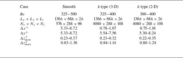


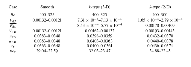


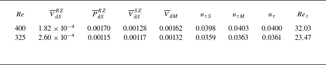


 Open access