


I. INTRODUCTION
The intrinsic mechanisms available to a material to accommodate an imposed loading condition depend on the state of long range ordering of the material from the atomic scale up to the structural length scale. A vast body of the literature has accumulated on how the equation of state relating pressure, volume, temperature, and internal energy can be mapped from experiments involving the use of strong impulsive loading conditions.Reference Walsh and Christian1–Reference Knudson, Hanson, Bailey, Hall, Asay and Anderson7 A rigorous understanding of wave propagation, both elastic and plastic waves, through bulk solids underpins this field. Tremendous strides have also been made in relating the passage of high amplitude shock waves with the evolving state of the material’s microstructure, principally through post mortem observations and development of constitutive laws for plastic deformation.Reference Steinberg, Cochran and Guinan5,Reference Follansbee and Kocks8,Reference Andrade, Meyers, Vecchio and Chokshi9
Of more recent interest are long-range periodic lattice structures with symmetry operations normally associated with crystal lattices at the atomic level while being fabricable at a variety of length scales, from order of nanometers to millimeters. Recent advances in additive manufacturing (AM), for instance, have enabled heretofore unrealizable geometric and topological structures with novel properties and excellent scaling behavior associated with elastic properties, for instance. An explosion of interest in the fabrication of such architected structures has been followed by significant understanding of the static properties associated with them.
There is also considerable interest in the community to exploit such architected structures as wave guides with optimized band gap propertiesReference D’Alessandro, Belloni, Ardito, Corigliano and Braghin10,Reference Wang, Zhang, Zhang and Hu11 or in energy damping applications.Reference Schaedler, Ro, Sorensen, Eckel, Yang, Carter and Jacobsen12 What is lagging behind is our understanding of wave propagation in such structures, particularly in the context of high amplitude stress waves that are encountered under dynamic loading conditions, where the wavelengths are comparable in scale to the lattice structure of interest. The dynamic compression response of such lattice materials is not obvious owing to the geometric complexity. Shock wave interactions throughout the lattice and with free surfaces require new measurement techniques to follow the wave propagation, and thus understand the deformation response.
Dynamic compression of materials viewed through traditional shock physics experiments have often had to rely on integrated macroscopic measurements such as photon doppler velocimetry, PDV,Reference Strand, Goosman, Martinez, Whitworth and Kuhlow13–Reference Dolan15 and velocity interferometer system for any reflector, VISAR.Reference Barker and Hollenbach16 These experiments have been very successful in the shock physics community in routinely determining equation-of-state information for materials despite underlying assumptions required with macroscopic measurements.Reference Meyers17 A large body of work has gone into inferring local phenomena from these measurements by coupling with advanced simulation and materials modeling efforts. Often phase transitions inferred from PDV or VISAR measurements are cross-validated with diffraction measurements of materials in the diamond anvil cell, DAC.Reference Jayaraman18 Furthermore, combining tradition shock physics experimental techniques with other measurement modes such as a high-speed imaging allows for better constraints to be placed on the models if they must capture both the integrated response as well as the local geometric evolution.
The phase diagrams produced by quasi-static and dynamic deformation do not always agree,Reference Yoo, Akella, Campbell, Mao and Hemley19–Reference Ahrens, Johnson and Ahrens21 making the direct observation of material evolution under dynamic conditions preferable.
Combining these techniques allows for direct one-to-one comparison and frees us from some underlying assumptions such as samples being bulk solids. The large number of interactions of a mechanical wave through geometrically structured lattice materials makes an integrated measurement challenging to infer local kinetics or local phenomena.
This has been addressed to a degree in recent publications by Hawreliak et al.,Reference Hawreliak, Lind, Maddox, Barham, Messner, Barton, Jensen and Kumar22 Winter et al.,Reference Winter, Cotton, Harris, Maw, Chapman, Eakins and McShane23 and Branch et al.,Reference Branch, Ionita, Clements, Montgomery, Jensen, Patterson, Schmalzer, Mueller and Dattelbaum24 whereby the dynamic compression response of lattices or other long-range periodic structures was elucidated. Studying the dynamic compression of such heterogenous open structures requires a more spatially resolved targeted diagnostic. New facilities such as the Dynamic Compression Sector (DCS) at the Advanced Photon Source (APS) are allowing researchers interested in the dynamic deformation of materials unprecedented access to observables at a local level through ultra-fast direct X-ray absorption, X-ray phase contrast imaging (PCI), and X-ray diffraction measurements.Reference Gupta, Turneaure, Perkins, Zimmerman, Arganbright, Shen and Chow25 These measurement techniques allow for probing the targeted material state in space and time including but not limited to such phenomena as direct imaging of spall formation, pore collapse, jetting, crack propagation, fracture, and diffractive imaging of local phase content, phase transitions, strain (stress) state, and dislocation content.
Now that a platform exists for probing local deformation response of materials at high strain rates, one is not limited by the assumptions of homogeneity, and we are able to study the deformation response of heterogeneous structures, such as lattice materials produced via AM. With this new mindset of manufacturing and measurement capabilities in high strain rate regimes, we seek to combine the techniques to gain a more detailed understanding of the temporally and spatially resolved deformation behavior of these materials. These regimes represent conditions where such behavior is unknown and not well-understood. In situ investigation of AM lattices under dynamic compression is beginning to gain interest in the community as experimental platformsReference Eakins and Chapman26 and complementary simulationsReference Winter, Cotton, Harris, Maw, Chapman, Eakins and McShane23 are coming on-line to investigate such phenomena.
Recently, Hawreliak et al.Reference Hawreliak, Lind, Maddox, Barham, Messner, Barton, Jensen and Kumar22 showed the existence of an elastic precursor wave in polymer lattice materials as a function of lattice orientation for fixed impact speed, impacting material, and observation times soon after impact. Numerical and experimental studies of the dynamic compressive response in structured and unstructured porous materials, such as 2D lattices and stochastic foams, have shown signs of elastic wave propagation in metals.Reference Winter, Cotton, Harris, Maw, Chapman, Eakins and McShane23,Reference Petel, Ouellet, Frost and Higgins27–Reference Zou, Reid, Tan, Li and Harrigan30 The amplitude and pressure of an elastic precursor is generally much higher in metals compared to polymers. During shock loading, the observation of an elastic precursor will depend on the driving pressure.Reference Meyers31,Reference Taylor and Rice32 The elastic precursor wave is an elastic compressive wave that transmits the applied pressure atom by atom. The observation of such phenomena in metals has been documented for more than half a century, and this phenomenon is one of the classical observations in shock physics. Dynamic compression at even higher pressures will induce overdriving whereby the plastic wavespeed (which depends on driving pressure) overtakes the elastic wavespeed (pressure independent).Reference Dunn and Fosdick33 In the case of both elastic and plastic waves, the elastic wavespeed is faster than the plastic wavespeed; however, it is the change in particle speed that relates to the pressure state of the individual wave. Elastic waves have low particle speeds and associated low pressures as opposed to plastic waves with higher particle speeds and pressures. When the pressure allows for both elastic and plastic waves, it has been observed that an elastic precursor can decay significantly with propagation distance in bulk materials. Furthermore, free surfaces typically lead to reflections that complicate the propagation of an elastic precursor.
Following from this recent work, a few open questions arose regarding the nature of the elastic precursor evolution at longer time and larger propagation distances as well as for different impact conditions. Specifically, will the elastic precursor in a polymer lattice decay rapidly as in dispersive open structures such as granular materials? And, is the elastic precursor speed independent of impact speed, as is typically observed in bulk solids? In this study, we track the evolution of the elastic precursor wave in an AM octet lattice subject to dynamic compression via gas gun driven flyer impact and monitored through time and space via PCI. We perform direct numerical simulations to compare with our experimental observations and elucidate those observations.
II. MATERIALS & METHODS
A. Sample fabrication
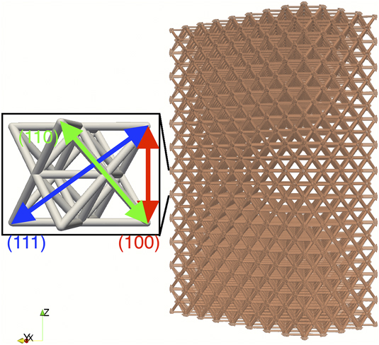
The samples tested were made of solid, fully polymerized, 1,6-hexanediol diacrylate (HDDA) polymer with all having a relative density of 10% and fabricated by projection stereolithography,Reference Hull34–Reference Zheng, Lee, Weisgraber, Shusteff, DeOtte, Duoss, Kuntz, Biener, Ge, Jackson, Kucheyev, Fang and Spadaccini37 an AM technique. The samples were built as 3D arrays from octet truss unit cells in the (100) orientation. Each unit cell volume was on the order of (250 µm)Reference Ahrens3. For practical purposes of the experiment to be performed, these were built in 4 × 8 × 8 and 4 × 8 × 12 unit cell arrays with corresponding physical sizes 1 mm × 2 mm × 2 mm and 1 mm × 2 mm × 3 mm, respectively. The unit cell size and relative density correspond to having ligament lengths of 177 µm and ligament diameters of 21 µm. Different height samples were tested to pair the maximum elastic precursor wave propagation distance with duration of the test. Figure 1 represents an idealized version of the 4 × 8 × 12 octet lattice that was built and tested.
Idealized 4 × 8 × 12 octet lattice shown on the right. Impact direction is along the (100) direction, or alternatively z-direction (shown vertically). A zoomed in depiction of a single octet unit cell is shown to the left. For scale, actual as-built sample is 3 mm tall in z.
B. In situ imaging during dynamic compression
Each of the described samples were imaged using PCI. They were mounted in the IMPULSE single stage gas gunReference Brown, Ramos, Dattelbaum, Jensen, Iverson, Carlson, Fezzaa, Gray, Patterson, Trujillo and Martinez38–Reference Ramos, Jensen, Yeager, Bolme, Iverson, Carlson and Fezzaa43 and static preshot frames taken. A more detailed description and schematic of the gas gun system and detector system can be found elsewhere.Reference Jensen, Luo, Hooks, Fezzaa, Ramos, Yeager, Kwiatkowski, Shimada and Dattelbaum39 The detector setup at DCS allows for 8 PCI images to be taken of the same sample at short time intervals between frames. Timing of an individual frame is synchronized with the X-ray beam, and this sets the minimum time interval between successive frames. For the standard 24 bunch mode used at APS for these experiments, this effectively places the minimum time interval between successive frames at 0.153 µs. Each electron bunch is 33.5 ps in duration, giving an almost instantaneous flash X-ray image of the sample material for each frame. A cerium-doped lutetium oxyorthosilicate, LSO, scintillator is optically coupled through a series of mirrors to 4 distinct Princeton Instruments PI-MAX4 1024-f cameras. Each camera is able to take two frames per experiment. With focusing optics utilizing a 7.5× objective, these detectors each have an effective field of view (FOV) of 1.726 × 1.726 mm containing 1024 × 1024 pixels with a corresponding effective pixel size of 1.686 µm. The effective pixel size sets the smallest feature size, or resolution, of the experiment. During each shot, one PDV probe was utilized to measure the back surface velocity of the AM samples, and another PDV probe was offset to monitor the speed of the incoming flyer. As the open space in the lattice is transparent, in principle, these experiments could be performed with a similar loading platform, optical backlighting, and high speed cameras.
Each of the samples are dynamically compressed by using a gas gun driven flyer and imaged perpendicular to the compression direction at some time after the flyer impacts the sample surface (t = 0). The samples are compressed along the (100) direction and imaged along a  $\left( {0\bar{1}1} \right)$ direction. The flyer is much longer in length in the direction of the shock than the lattice sample. If the flyer were shorter than the sample, one would need to consider release effects from the flyer. In that case, the pressure drive essentially switches off during the test. This would unnecessarily complicate the wave propagation interpretation. Table I details the sample size, impact speed, sample region of interest interrogated by the X-ray beam, starting time for observation of first frame of data for the set of 9 experiments, and the impacting flyer material. As the lattice sample is larger than the FOV, our approach was to perform two experiments for each impact condition. One experiment would probe the early-time response of the lattice sample by imaging the portion of the sample closest to the impact shortly after impact. The second experiment would probe the later response of the lattice sample by imaging the portion of the sample further downstream of the flyer at later times. While these sets of data are gathered from two slightly different impact speeds, the intent is to consider them as a single experiment having an equivalent response. We believe the good reproducibility from shot to shot of the impact conditions and samples fabrication is sufficient to make this assumption valid. The late-time deformation behavior of the sample incorporates the integrated effects of deformation from the early-time.
Sample geometry and shot description for the nine experiments performed. Sample size in number of unit cells is given, along with impact speed (v 0), time from impact to the first frame (t start), the distance along the impact direction the sample was viewed (d offset), impacting flyer material, and the propagation behavior being probed (either early or late time).

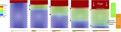
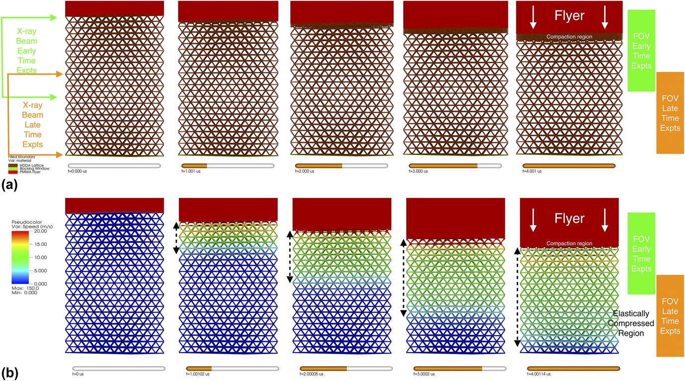
Figure 2 provides a combined schematic to portray the timing of the experiments and the kind of information gathered during early- and late-time experiments. The depiction of the lattice deformation is from the simulations to be discussed in Sec. II.C. Figure 2(a) shows the progression of a poly(methylmethacrylate) (PMMA) flyer as it compacts the HDDA lattice at 1 µs snapshot intervals. For the early experiments, the X-ray beam and PCI FOV is focused on the portion of the sample closest to the impact surface. In these simulations, we observe the formation of a compaction region. Figure 2(b) depicts an elastically compressed region where the local material, or particle, speed (dashed black arrows) is small. The wave front for this region runs ahead of the compaction region. The wave front is the interface between elastically compressed and uncompressed portions of the lattice. The effects of the small particle speeds can be observed experimentally by the relative motion of that portion of the lattice. After 2 µs, the wavefront between the elastically compressed region and uncompressed region passes the edge of the early-time experiment FOV. We are interested in the propagation of the elastic wave, and so to track the wave at later times required a late-time experiment FOV that was further downstream of the impact direction. In the slower impact speed tests like the one depicted here, the flyer and compaction region never enters the experimental FOV for the late-time experiments.
Snapshots every 1 µs from the simulation of a 4 × 8 × 12 HDDA octet lattice impacted at 150 m/s by a PMMA flyer viewed from the  $\left( {0\bar{1}1} \right)$ direction (Simulation #1 in Table II corresponding to Experiments #1 and #2 in Table I). The regions of the sample imaged during the early and late time experiments are depicted in green and orange by FOVs translated along the impact direction. (a) the lattice closest to the flyer begin to form a compaction region. (b) the local material speed on a reduced scale from 0 m/s to 20 m/s to highlight the elastically compressed region running ahead of the compaction region. Material moving at 10 m/s, for example, over the interframe time of 0.153 µs will move 1.53 µm, or roughly one pixel in the experimental images.
For each experiment, 8 preshot images were also taken of the AM octet lattice prior to beginning the experiments. These images serve a dual purpose; the first is providing a comparison against the compressed state during the experiments and the second is providing a way to register the distinct views that each camera has.Reference Lind, Jensen and Kumar44 Also, a set of 8 static images of the direct beam were taken to obtain absorption images that could be used to estimate densification. These are images of the direct X-ray beam with the sample taken out of the X-ray beam path.
As an example, Experiment #5 listed in Table I was performed on a 10% relative density octet lattice in the (100) orientation built from 4 unit cells long by 8 unit cells wide by 8 unit cells tall along the compression direction. This 1 mm × 2 mm × 2 mm sample was impacted by a flat-faced Al-6061 flyer at 288 m/s, as measured by the PDV probe pointed at the flyer surface. The X-ray beam and consequently 4 cameras were focused on a region of interest of the sample with the surface of the sample at the leftmost edge of the frame. By our convention, the flyer enters the FOV from the left edge of the frame. The first frame in the 8-frame sequence is obtained at 0.650 µs after the flyer face impacts the sample surface. Each successive frame is 0.153 µs after the previous one.
Figure 3 shows a few of absorption images obtained from Experiment #5 after applying bright field and registration corrections. The images shown are frames 2, 4, 6, and 8 in the sequence of 8 frames. The dashed, colored lines in Fig. 3(e) represent the location of the flyer face in each of the 8 frames taken during impact. From the images shown in Fig. 3, one sees evidence for the plastic/compaction wave in the compaction/densification of the lattice that lies ahead (to the right) of the flyer. Red marker arrows are added to denote the left and right edge of the compaction region. In the images, the flyer comes in from the left. The left edge of the compaction region represents the interface between the flyer and compaction region. The right edge of the compaction region represents the interface between the compaction region and the mainly intact lattice. We will refer to this as the compaction wavefront or compaction front. The structure of the lattice is still somewhat discernible in the compaction region, albeit as the open space is squeezed out of the lattice as it is crushed. Further to the right of the compaction region, small deflections of the struts and nodes can be observed. These observations are indicative of an elastic precursor wave running ahead of the plastic wave. These deflections serve to slightly (elastically and uniaxially) compress the lattice while it remains intact. The last subfigure, Fig. 3(e), serves to highlight the deflection of the nodes through the sequence of frames. The positions of the nodes are plotted as colored dots with dark blue representing where the nodes are in the static frame, lighter blue corresponding to the earliest experimental frame continuing on to red in the last frame. One sees only dark blue dots in the left edge of the figure as those nodes and that material of the sample become part of the compaction region by the time of the first frame. The compaction wave has already swept through this portion of the sample by the first frame, 0.650 µs after impact. In the middle of the figure, one can see color gradations which are indicative of the small motions of the nodes. Finally, the nodes in the right edge of the figure fall on top of one another indicating no apparent motion experimentally. This tells us that the compression of the lattice by the elastic precursor wave has not reached this part of the sample by the end of the experiment. The visual flow of the dots represents the trajectory of those material points at discrete points in space and time. They represent the effects of an elastic precursor running ahead in the lattice. The interface between the elastically compressed region and uncompressed regions will be referred to as the elastic precursor wavefront.
(a)–(d) 4 of the phase contrast images from the sequence of 8 obtained for Experiment #5 on AM lattice structures using IMPULSE. Timing between frames is synchronized with the electron bunch structure at the APS, 0.153 µs between electron bunches. (e) A depiction of the progression of the flyer (dashed lines) and position of all nodes in the material through the sequence of images. Blue represents the information from the earliest measured static frame. Red represents information from the last measured frame, 1.071 µs after the first frame or 1.721 µs after initial impact. The FOV presented in each figure is 1.726 × 1.726 mm.

The remaining eight experiments as detailed in Table I were carried out in similar fashion. Experiment #1 in Table I represents a low speed impact of a flat-faced PMMA flyer while imaging the lattice closest to the impact surface at times shortly after impact. Experiment #2 represents the same requested impact conditions (impact speed and material) as Experiment #1 with the only difference being that the FOV is farther downstream of the impact and the experimental frames at later times after the initial impact. The X-ray beam is fixed and so to move the FOV involved placing the front edge of the sample at the left edge of the FOV, and then translating the gun a prescribed distance perpendicular to the X-ray beam direction. The movement of the entire system was performed in sequential steps and monitored via both a micrometer and X-ray imaging to precisely move the sample a prescribed distance along the compression direction. This experiment along with the first are assumed to behave the same way such that the second experiment gives us the later time, or equivalently longer propagation distance, behavior of the lattice. Experiments #3 and #4 repeat the same procedure as #1 and #2 at the same impact speed but with a higher density, higher mechanical impedance flyer, Al-6061. Experiments #5 and #6 repeat the same procedure with a higher impact speed than #3 and #4. In the case of Experiment #6, we failed to obtain a PDV signal for the projectile, so we can only estimate the impact speed based on the requested impact speed. Typically, the difference observed between requested and measured impact speed is not more than 5%. Experiments #7 and #8 repeat the same procedure with an even higher impact speed than #5 and #6. Finally, Experiment #9 repeats the same procedure with an even higher impact speed than #7 and #8. The offset distances in the later experiments were an attempt to capture effects of dispersion of the elastic wave. In some of the later experiments, the effects of the elastic precursor wave are not apparent in all of the frames as its arrival was later than originally anticipated.
C. Simulations
Complementary finite element simulations were performed in ALE3D, an arbitrary Lagrangian Eulerian finite element code developed at Lawrence Livermore National Laboratory.Reference Noble, Anderson, Barton, Bramwell, Capps, Chang, Chou, Dawson, Diana, Dunn, Faux, Fisher, Greene, Heinz, Kanarska, Khairallah, Liu, Margraf, Nichols, Nourgaliev, Puso, Reus, Robinson, Shestakov, Solberg, Taller, Tsuji, White and White45 The simulations were performed on a 4 × 8 × 12 polymer octet lattice with a relative density of 10%, see Fig. 1. The material properties used in the simulations for the base lattice material are given in Table SI. Five simulations were performed for the entire time frame observed in the experiments (up to 4.0 µs) at impact speeds of 150, 300, 530, and 700 m/s with impacting materials matching those listed in Table I. The first simulation in Table II corresponds to Experiments #1 and #2 in Table I. A mesh resolution of 2.5 µm was used, resulting in more than 500 × 106 hexahedral elements after incorporating flyer and backing material to the simulations. Figure S1 provides a depiction of the fidelity of the mesh used by showing the mesh for an octet truss single unit cell. This represents ∼9 elements across the ligament diameter or equivalently 100k mesh elements describing a lattice unit cell. The simulations were run using an explicit integration scheme, and to ensure stability, the time step is controlled by a fraction of the Courant condition. In the simulations containing Al-6061 flyers, the time step was approximately 0.25 ns. In the simulation containing a PMMA flyer, the time step was approximately 0.625 ns. The shorter time step in the prior simulations is a direct consequence of the higher sound speed in the Al-6061 effectively controlling the time step. The simulations are run using a mixed element advection schemeReference Noble, Anderson, Barton, Bramwell, Capps, Chang, Chou, Dawson, Diana, Dunn, Faux, Fisher, Greene, Heinz, Kanarska, Khairallah, Liu, Margraf, Nichols, Nourgaliev, Puso, Reus, Robinson, Shestakov, Solberg, Taller, Tsuji, White and White45 as opposed to explicitly modeling contact. Material interfaces are inferred. The model used here does not incorporate viscoelastic and viscoplastic effects. These effects could influence the simulated deformation response but were not investigated in detail.
Geometry and impact conditions for the four simulations performed. Sample size in number of unit cells is given, along with impact speed (v 0), impacting flyer material, and direct correspondence with experiments performed in Table I.

We attempted to match the output of the simulation at the same length and time scales present in the experiment and use the same methodology to compare elastic precursor evolution. In the simulation, position gauges were placed at every node position. The displacement information for each gauge is sampled every 0.153 µs to best mimic the discrete time nature of the experimental measurement. Furthermore, gauges could have been placed throughout the sample rather than in discrete locations (nodes), but again the motivation was to best mimic the experimental measurement.
Figure 2 shows the results from Simulation #1 in Table II of a PMMA flyer impact on a 4 × 8 × 12 HDDA octet lattice at 150 m/s. Over the 4 µs simulation time, a compaction region and elastically compressed region are seen to develop. One sees that the local material speed in the elastically compressed regions is much lower than that in the compaction region, and the compaction wavefront speed is slower than the elastic precursor wavefront speed. The behavior observed in the simulations, compaction of the lattice with an elastic precursor wavefront running well ahead of it, is qualitatively similar to the experimental observation.
III. ESTIMATES OF THE ELASTIC PRECURSOR EFFECTS ON THE LATTICE FROM EXPERIMENTAL AND SIMULATED DATA
In the experiments, one observes evidence for small deflections of nodes and deflections of ligaments ahead of the compaction front. These deflections are an observable signature of an elastic precursor wave running ahead of the compaction wave. The region between the elastic precursor wavefront and the compaction wavefront is an elastically compressed portion of the lattice. The extent and boundaries of this region evolve with time as the elastic precursor wavefront and compaction wavefronts sweep through the lattice sample in time. At early times in the experiment, one has three different states of the lattice at a given instant in time, that being compaction, elastic compression, and undisturbed material. The individual wavespeeds and sample lengths set a minimum time in which the end of the sample will respond to the incoming wave.
We have taken an approach to track the lattice nodes in the sequence of images as a way of studying the propagation of an elastic wave through the lattice material. Our position gauges in the simulations capture this information as well. To quantify the deflections and displacements of lattice nodes due to the elastic precursor wave, one needs first to identify the starting position of each node in the experimental static images. This was performed by generating a template node image and performing pattern matching of the template node image with the static image.Reference Lind, Jensen and Kumar44 This automatically identified regions in the static image which were most similar to the template node image. We then implemented a cross-correlation-based particle tracking methodReference Scarano46 to follow the position of nodes throughout the experimental frames. The result of such node tracking results in a node trajectory as presented earlier in Fig. 3(e). A node can fail to be tracked in later experimental images if the nearby region is no longer qualitatively similar to the region in the previous frame. Quantitatively, this corresponds to when the local cross-correlation falls below a threshold of 0.5. This is the case, for example, when the compaction front sweeps through a set of nodes. It is noted that the local cross-correlation drops precipitously when nodes become compacted making 0.5 an appropriate threshold. After processing the experimental images, one has a list of node trajectories for each node in the lattice that is specified by the physical position (x im, y im), time of observation, t, including at t = 0 (from the static frame), some binary notion of whether the node has a cross-correlation that has fallen below the threshold and likely lost into the compaction front, and a node number, n. x im is defined as the impact direction (horizontal direction in the experimental images), and y im is a direction lateral to the impact direction (vertical direction in the experimental images). As the experimental images are X-ray projections, it is not possible to determine node position along the X-ray beam, z im. The total amount a fully tracked node n has moved by time t from its initial position at t = 0 can then be calculated.
At this point, the node trajectories from the experiment are specified almost exactly in the same manner as the position gauges from the simulation. Displacements parallel to the equivalent X-ray beam direction are ignored from the position gauges. Position gauges initially lying along the equivalent X-ray beam direction are averaged into a single node trajectory. The transition of nodes from being in an elastically compressed region into the compaction region can be noted by an abrupt increase in local material speed giving rise to a sharp change in displacement.
Figure 4 presents the node trajectory data from Experiments #1 and #2 with Simulation #1 as well as Experiments #7 and #8 with Simulation #4. The results from the paired experiments are shown side-by-side. The equivalent simulation data are presented below the experiment results with a schematic of where the equivalent experimental FOV was placed. Node positions are colored by time point where blue corresponds to the earliest time point and red corresponds to the latest time point. The node trajectories in the experiments have a maximum of 9 time points, whereas the simulation has 27 time points. In both cases, an estimate of the elastic precursor wavefront at a given time point is plotted as dashed vertical lines. Blue corresponds to the earliest time point and red to the latest time point. For these plots, the estimated elastic wavefront position is based off of where the nodes have been displaced from their original position by more than 3 µm. This displacement cutoff is chosen because it is close to the resolution limits of the experimental measurement. This represents, in some sense, a small but reliable displacement measurement in the experiment. The two impact conditions highlighted in these figures represent extremes in impact conditions reported spanning slow impact with a lighter, softer material to faster impact with a denser, harder material. One can see that in general a node remains in the elastic precursor (and out of the compaction front) for more time points in the slower, lighter impact condition. The compaction front is moving faster in the faster impact and so nodes are more rapidly added to the compaction front. The width of the elastically compressed region of the lattice is a function of observation time as well as the difference between the compaction front speed and elastic precursor wave speed. The simulations show qualitatively equivalent movement of the elastic precursor wavefront over the same period of time and same sample length. It is difficult from this figure to compare across experiments as the FOVs are different and the starting times are different.
Node trajectories for Experiment #1 in (a), Experiment #2 in (b), Simulation #1 in (c), Experiment #7 in (d), Experiment #8 in (e), Simulation #4 in (f). Dashed lines represent an estimate of the wavefront based off of a 3 µm movement of nodes. Colors denote the time in the experiment or simulation with blue indicating early and red indicating late.

The average wavespeed from frame to frame is then simply the differential movement of the wavefront position divided by the interframe time, 0.153 µs. Note that while the elastic wavefront sweeps out a large distance over the course of the experiment, the individual node movements are minimal. The movement in the wavefront appears somewhat jerky in the experiments and can be due to the discrete nature of the points in space and time and any error in the nodal position estimate. This error should be random and not systematic, and so if we look at the wavefront trends across the experiments, one might expect a clearer pattern for the wavefront evolution to emerge. Given the smallest measure of displacement here is 3 µm (which is rather large compared to interatomic spacings), strictly speaking, this wavefront is the smallest and fastest detectable experimental evidence of the elastic precursor. This is part of the material in the elastically compressed region but does not represent the boundary between elastically compressed lattice and uncompressed lattice, technically the elastic precursor wavefront.
Recalling that the pixel size in these experiments is 1.686 µm, a 3 µm motion between frames is less than 2 pixels. The cutoff used here effectively defines a minimum average interframe velocity for the nodes, often referred to as particle speed. A 3 µm detectable motion in one interframe time period (0.153 µs) corresponds to a minimum average speed of 20 m/s. By definition, the elastic precursor is a low amplitude, low pressure wave with accompanying low particle speeds.
When considering shock wave propagation through a material, one needs to consider the particle speed and wave speeds to apply the fundamental Hugoniot relations. In these experiments, the nodes are analogous to the concept of the particle (or local material volume). A wave, on the other hand, is a coordinated movement of material. While the previous figure provides a good pictorial representation of the node motion (and particle speed), it required an interpretation to infer the coordinated motion by using a cutoff to locate a wavefront. A simple toy problem to consider is a 1-D square wave with speed U and particle speed u p traveling through a material from left (x = 0) to right for time, ∆t = t 1 − t 0, in a fixed lab frame. In this time, the wave will have moved a total distance of U × ∆t. The material originally at x = 0 will have displaced by u p × ∆t. However, the material at x = U × ∆t has yet to move at t 1 and will begin to move at u p immediately after t 1. If one considers the particle displacement versus lab position at a given time (say t 1), a displacement profile will show a straight line from u p × ∆t to 0 across a distance of (U − u p) × ∆t. For small u p compared to U, the slope of the line is u p/U and represents the volume compression of the material, called η, or nearly equivalently the uniaxial strain in the compression direction, or εc. The volume compression is a measure of the amount of compression a specific compressive wave has on the material.
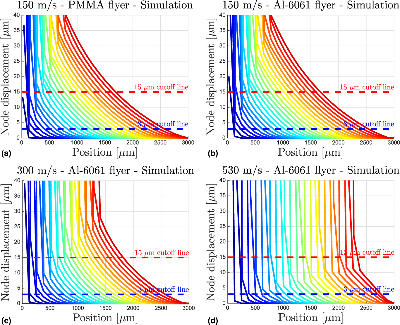
In this spirit, we take the node trajectory data to construct displacement profiles as a way of visualizing the action of an elastic precursor as it sweeps through our lattice. The slope of the displacement profile will inform us on the amount of uniaxial compression the lattice is subjected to in the elastically compressed region. At any discrete timepoint, we have a measure of the node movement, d(t, n); however, these points are also discrete in space. One would like to have a continuous displacement field for a fixed time point. To overcome this, we estimate the displacement at any given point in space for a fixed time by linear interpolation of the displacement values of the nearest nodes. Since we are primarily interested in the lattice compression along the compression direction, one can average this field across the y im-dimension to produce a displacement versus position profile similar to as described in the toy problem in the previous paragraph. Figure 5 presents the displacement profiles for Experiments #1, #2, #7, and #8. For completeness, the displacement profiles for the remaining experiments are provided in the Supplementary Material in Fig. S2. Each color-coded curve represents the displacement of the lattice versus the lab position at a given instant in time. Blue curves represent the earliest times in the experiment progressing to red which is the latest. Recall that the flyer and also compaction front sweep in from the left to the right. An estimate of the initial position of the compaction front from the experimental images at the earliest frame is denoted by a blue X mark on the horizontal axis. The last position of the compaction front from the experimental images at the last frame is denoted by a red X mark. For Fig. 5(c), the compaction front never enters the experimental FOV. The continuous curves represented here are derived from displacements of nodes (discrete points in space). For the reader reference, the lattice is aligned such that the first set of nodes lies nearly at the origin. From the lattice unit cell size and orientation, this places each successive set of nodes at increments of 125 µm. The curves represent the evolution of the elastically compressed region, where the left edge of the curve likely is close to the interface between the compaction region and elastically compressed precursor region. The right edge would represent the elastic precursor wavefront which is the interface between the elastically compressed region and the uncompressed region of the lattice. Dashed lines are also presented to guide the reader to where one might predict the wavefront is for a given displacement cutoff. Finding the intersection of the dashed line with the colored curve is then the estimated wavefront position at that given observation time. Black dots are overlaid on Fig. 5(a) to show the change in position of the wavefront for cutoffs between 3 µm in 1 µm increments up to 15 µm. The displacement profiles in the lower speed experiment have much wider profiles. This is due to the fact that the compaction front is moving much more slowly allowing for a larger width of the elastically compressed region to develop earlier in time.
Displacement profiles depicting the average nodal displacement as a function of lab position along the sample for Experiment #1 in (a), Experiment #2 in (b), Experiment #7 in (c), and Experiment #8 in (d). Blue dashed lines represent an estimate of the wavefront based off of a 3 µm movement of nodes. Curves are color coded by the experimental observation time.
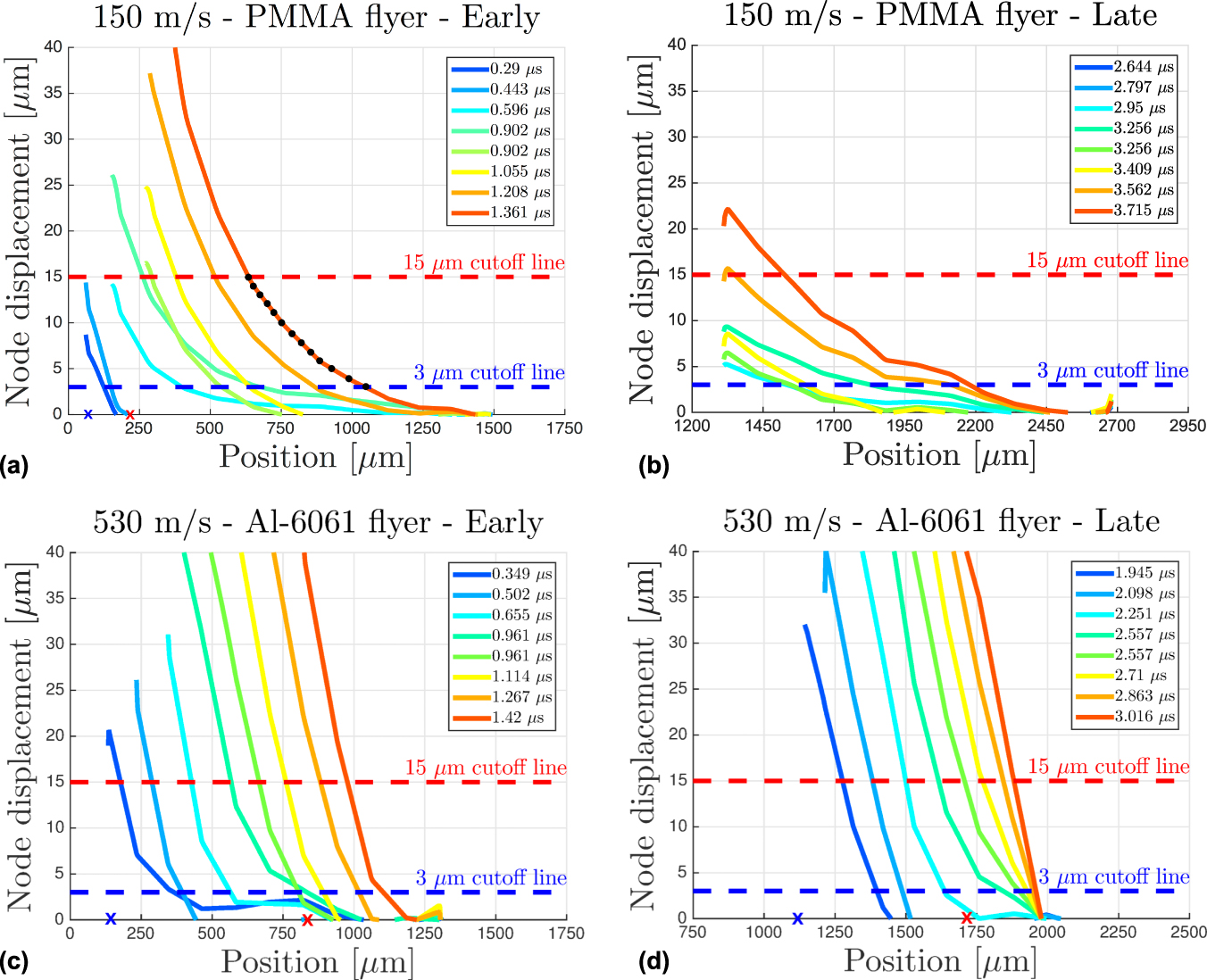
Figure 6 presents the displacements profiles from the four simulations in the same manner and vertical scale as Fig. 5. One notes the gradual nature of the curves going from right to left with an abrupt increase at some point. The gradual increase in the curve at the foot of the curve is indicative of the elastic precursor effects. The rapid rise in the curve is simply the point at which nodes enter the compaction region in the simulations. The compaction region has a typically higher pressure and associated higher particle speed which give rise to rapid displacement increases. Determining the position of the compaction front from the simulation’s displacement profile is much easier to discern from these figures, and they provide an informative comparison against the experimentally derived curves. One could extract the compaction front position versus time from these profiles and find the compaction speed; suffice it to say, the slope of that interface between smoothly varying and rapidly varying portions in these displacement profiles is directly proportional to the compaction speed. The smoothly varying portion of the curves can be associated with the elastically compressed region and the width of these profiles at a similar time point across simulations decreases with increasing impact speed. Interestingly, their heights also correspondingly decrease. One sees that the elastically compressed region of the lattice can be quite large (>1 mm) for low impact speeds at later times; however, this zone is on the order of a unit cell size or two for the higher impact speed (530 m/s). Qualitatively, the profiles are quite similar except for the truncation on their left edge by the compaction front. For all the time points in the 530 m/s simulation, a 15 µm cutoff line defines a wavefront in the compaction region, and therefore not in the elastically compressed region.
Displacement profiles depicting the average nodal displacement as a function of lab position along the sample for Simulation #1 in (a), Simulation #2 in (b), Simulation #3 in (c), and Simulation #4 in (d). Curves are color coded by the simulation times spaced at 0.153 µs intervals. The first blue curve corresponds to 0.153 µs after impact while the last red curve corresponds to 3.978 µs after impact.
Standard analysis of wave propagation through materials will include an x–t diagram to visually depict the location of various wavefronts to show wave reflections and interactions. The horizontal axis, or x-axis, is typically the position along the compression direction. The vertical axis, or t-axis, is the time axis starting at initial impact when t = 0. One thing to note is that lines in x–t diagrams with larger slopes correspond to slow moving wavefronts and conversely smaller slopes correspond to fast moving wavefronts. Figure 7 presents the data from the simulations from Fig. 6 represented as an x–t diagram. Each horizontal set of colored dots corresponds to a single displacement curve which are defined at a specific snapshot in time. The blue dot denotes at that specific snapshot in time where the 3 µm cutoff line intersects the displacement curve. The red dot denotes at that specific snapshot in time where the 15 µm cutoff line intersects the displacement curve. The solid black line with black circles represents the position of the flyer with time. The black circles are presented at discrete time intervals spaced 0.153 µs apart as the simulation data were discretized in time to match the experimental time intervals. At a given vertical position (fixed time) in the x–t diagram, there are red through blue dots horizontally spread out. These represent some part of the elastically compressed region at a singe point in time. The red dots are placed at the position where the 15 µm cutoff line intersects that displacement profile at that time. The blue dots are placed at the position where the 3 µm cutoff line intersects that displacement profile at that time. The color gradation proceeds from a 3 µm cutoff (blue) in 1 µm steps to 15 µm cutoff (red). A single horizontal set of points in these x–t diagram represents an estimate of the wavefront position based on which cutoff is considered. For example, in the toy problem described above, the horizontal spacing of the points would be uniform as the u p was constant in the elastically compressed region. Bunched points are an indication of a strong particle speed change such as at the compaction front. The width of that elastically compressed region is then just the width those points take up. A gray window is added to indicate the fan in x–t space encompassed by those points. Finally, a set of black dots are placed at the position where the 1 Å cutoff line intersects that displacement profile at that time. These points represent what might be considered the elastic precursor wavefront position, but whose displacements are not able to be measured experimentally.
x–t diagram of the elastic precursor front for four simulated impact conditions. Projectile position is plotted in black lines while the elastic precursor front position is plotted with points. Blue thick points represent using a 3 µm cutoff while red thick points represent using a 15 µm cutoff for determining that nodes have moved. These points are directly determined from the displacement profiles, and each represents the intersection of an individual cutoff line with the displacement profile for a given snapshot in time. The shallow black thick points represent using a cutoff that is O (Å).
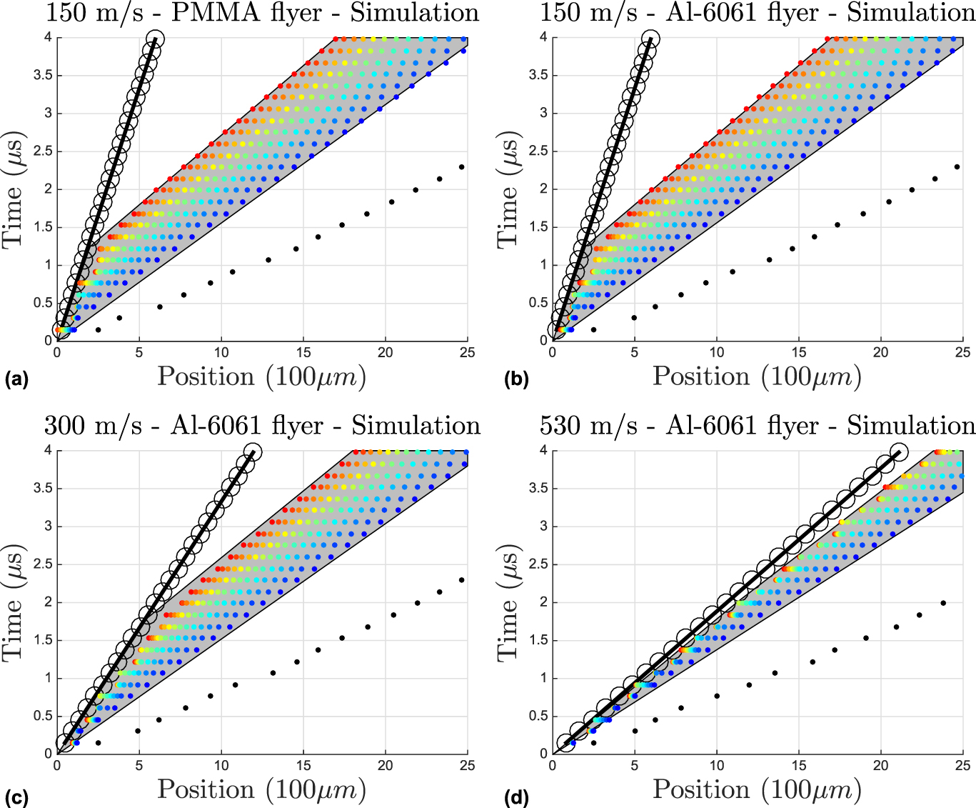
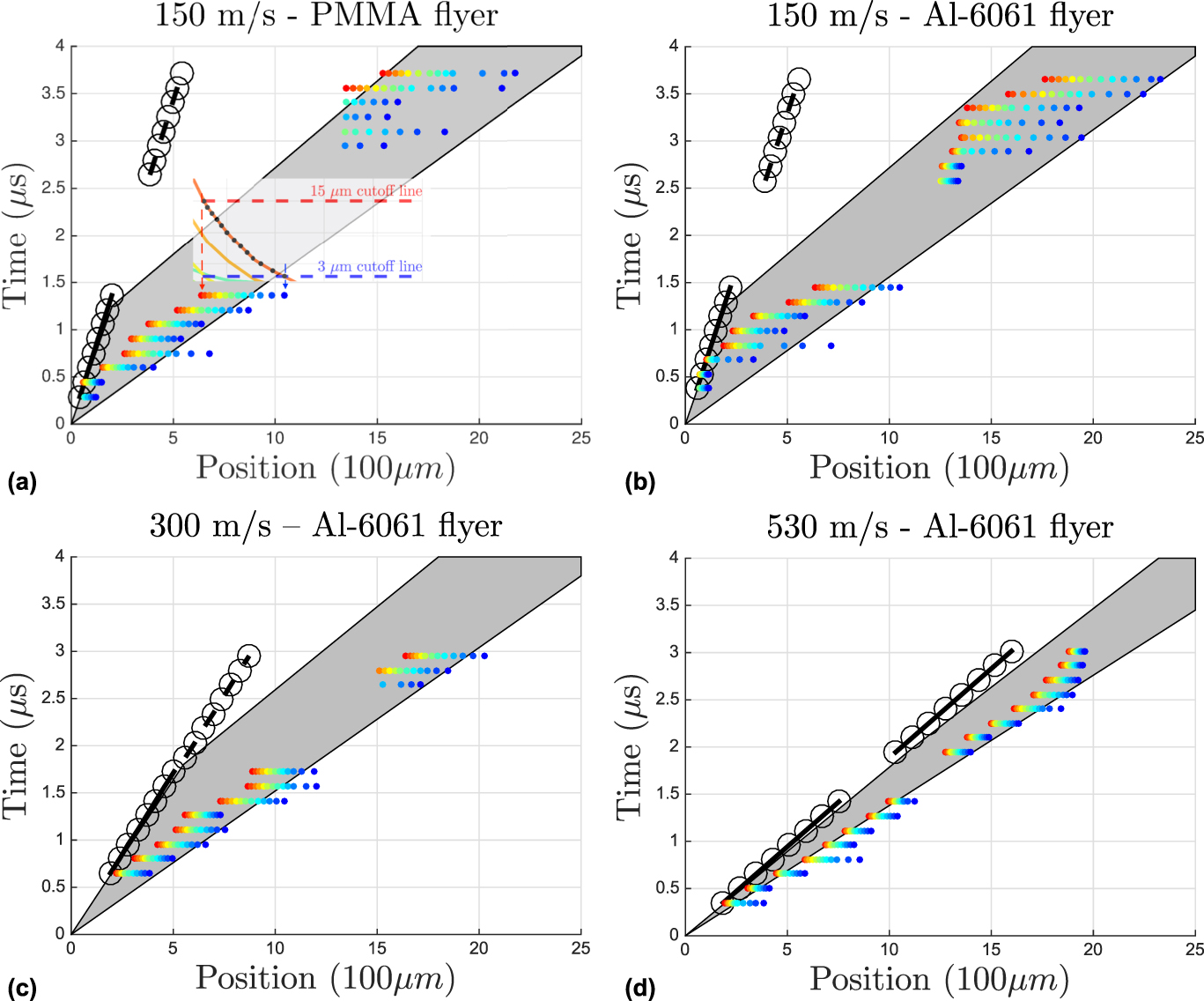
Figure 8 presents the data shown from the Experiments 1–8 in Table I (some partially shown in Fig. 5) represented as an x–t diagram. Experimental data from the paired experiments are now combined onto a single figure. A semitransparent portion of Fig. 5(a) is overlayed onto Fig. 8 to indicate how the intersection of a specific displacement cutoff line at a specific time and corresponding displacement profile result in the plotted points in the x–t diagram. A single displacement curve is defined at an instant in time corresponding to points along a horizontal line. The coloring of the points indicates which displacement cutoff is used. The gray fan included is the same fan taken from the complementary simulations. The projectile position is again plotted as a black solid (or dashed) lines with black circles. The black line is dashed for experiments where the flyer never enters the experimental FOV and so it is inferred from the experiment timing. The left edge of the gray window which lies closer to the compaction regions varies in slope from simulation to simulation, especially for the case of the 530 m/s impact, while the right edge of which is closer to elastic precursor wavefront is much more constant across impact conditions. The experimental data points seem to fall reasonably within the bounds predicted by the simulations. In some of the later time experiments, the effects of the elastic precursor were not observable until later frames in the experiment due to the FOV placement. In the figure, this is reflected by less rows of colored points in experiments performed at later times.
x–t diagram of the elastic precursor front and projectile position from all eight experiments. Projectile position is plotted in black lines while the elastic precursor front position is plotted with points. Blue thick points represent using a 3 µm cutoff while red thick points represent using a 15 µm cutoff for determining that nodes have moved. These points are directly determined from the displacement profiles, and each represents the intersection of an individual cutoff line with the displacement profile for a given snapshot in time. Black dashed lines indicate estimates of the projectile position from initial timing pin trigger as the projectile never entered the experimental FOV. The inset in (a) is a cutaway from Fig. 5(a) indicating the correspondence from displacement profiles to points on the x–t diagram.
Finally, Experiment #9 in Table I showed no experimental evidence for node deflections through multiple frames, and we will discuss this further in Sec. IV. We present Fig. S3 showing the equivalent node trajectory, displacement profiles, and x–t diagrams derived from Simulation #5. The gray fan in the x–t diagram is extremely narrow which is a proxy for width of the elastically compressed region which could be experimentally observed.
IV. RESULTS & DISCUSSION
Measuring elastic precursor wave arrival and speed via traditional shock physics velocimetry diagnostics in polymer lattices is extremely difficult owing to the open space of the lattices and the low particle speed of the wave. If the probe is not aimed directly at an interface between a node in the lattice and the reflecting backing surface, no velocity change will be measured. Furthermore, these particle speeds are small which make them difficult to extract because they produce a low frequency signal and thus require a longer time scale measurement. Typical velocimetry probes have extremely good temporal resolution (sampling rates of >25 GHz) as compared to the experimental image collection (6.5 MHz); however, measuring a small particle speed requires that particle speed to be fairly constant over a longer time window. For the imaging experiment, the effects of the elastic precursor are measured by variations in space at a given time, while for the velocimetry, the effects of the elastic precursor are measured by surface variation in time at a given position. The effects of the elastic precursor by way of movement of the nodes is unmistakable in the experimental images. The PDV (velocimetry) measurements we performed on those same samples were inconclusive. While the temporal resolution of the imaging experiment is very low compared to velocimetry measurements, the entire snapshot of the spatial response provides a rather strong and unique constraint to compare experimental data with simulation predictions.
From the displacement profiles in Fig. 5 and the x–t diagrams in Fig. 8 corresponding to the experiments, one sees that at similar experiment times, the wavefront physical spacing between the 15 µm cutoff wavefront and the 3 µm cutoff wavefront is much shorter for the higher impact speed experiment (#7 and #8 in Table I) as compared to the lower impact speed experiments (#1–#4 in Table I). The 15 µm cutoff wavefront can be interpreted as lying closer to or even in the plastic, or compaction, front, whereas the 3 µm cutoff wavefront can be interpreted as more toward the elastic precursor wavefront. In general, as the compaction wavespeed is increased, it begins to approach the material’s elastic wavespeed until a point at which the material can no longer support an elastic precursor. The compaction wave (pressure dependent wavespeed) overtakes the elastic wave (pressure independent wavespeed); this is typically called the point at which the material is overdriven.
As was noted earlier, the resolution limits of the experiment allow for measuring a minimally detectable wavefront which is not necessarily the elastic precursor wavefront. If the measurement allowed for atomic-scale resolution, the absolute elastic precursor wavefront could be pinpointed. The 3 µm cutoff wavefront has an average speed in the range of the experiments from 620 m/s to 755 m/s (a 135 m/s range), whereas the 15 µm cutoff wavefront has an average speed in the range of the experiments from 400 m/s to 720 m/s (a 320 m/s range). The lowest wavespeed in those ranges corresponds to the slowest impact and the highest speed to the fastest impact. In the above description of increasing compaction wavespeed approaching the elastic wavespeed, the largest cutoff wavefront speed would increase in the manner the compaction wavespeed is increased, while the smallest cutoff wavefront should change very little. From the trends observed, an increasing wavespeed would correspond to a decreasing cutoff value. This is consistent with our observation that the smallest cutoff wavefront is closest to the elastic wavefront and is less dependent on impact/compaction speed. The true elastic precursor wavefront will exhibit displacements on length scales much smaller than 3 µm, and so one expects that the spatial resolution limits will prohibit in some special cases the measurement of the effects of an elastic precursor even when one exists in the material.
Analyzing the cutoff wavefronts in the simulations, the 3 µm cutoff wavefront has an average speed in the range of the simulations from 635 m/s to 670 m/s (a 35 m/s range), whereas the 15 µm cutoff wavefront has an average speed in the range of the experiments from 420 m/s to 560 m/s (a 160 m/s range). Just as in the experiments, the larger cutoff wavespeed has the largest discrepancy across simulations, and the smallest cutoff wavespeed has a smallest discrepancy. Given the simulations have higher precision on displacement measurement, we extended Fig. 7 to include displacements at the Å level (black thick points). We find the curves for each of the simulations fall nearly exactly on top of each other with a measured speed of 1060 ± 45 m/s. As noted in Sec. 1, the interpretation of the elastic precursor is that of a compressive wave that transmits the mechanical stresses atom by atom. This measured speed is most likely the true elastic precursor speed.
From Fig. 7, the x–t profile begins to converge in both the experiments and simulations quickly as the chosen cutoff is decreased. The blue through red colored points represent a single order of magnitude decrease in cutoff while the difference between blue points and black points represent a decrease of 4 orders of magnitude. Experimentally, it is not feasible to measure such a large structure to angstrom resolution; however, comparing our experimental wavefront observation with complementary simulations at experimentally applicable resolutions allows for the estimation of the elastic precursor wavefront beyond the limits of the experimental resolution. There is agreement between the experiments and simulations in wavefront trends across experiments in the convergence of the wavefront speeds as the cutoff limit is decreased. Furthermore, there is general qualitative and quantitative agreement in the shapes, widths, and heights of the displacement profiles.
We observe for Fig. 8 that the experimental data points fall reasonable well within the simulation predictions (gray fan). The width of the profiles seems to match, and the agreement becomes worse as the compaction speed is increased causing a narrowing of the window of observations. For these higher impact experiments, to measure the effects of an elastic precursor on a lattice would require better spatial resolution as the largest displacements predicted in the elastically compressed regions become smaller and smaller until eventually smaller than the measurement resolution. For higher impact experiments, likely the temporal resolution would also need to be increased as the narrower width of the elastic region equally constrains the timescales.
The displacement profiles in Figs. 5 and 6 show a very gradual shape in the low velocity impact conditions. The high velocity profiles, both experimental and simulated, show a sharp rise most likely due to nodes transitioning into the compaction region. For the 150 m/s and 300 m/s simulations, the widths of the curves between the two extreme cutoff values represent a region of the lattice that is most likely fully contained in the elastically compressed region. It does not represent the full extent of the elastically compressed region, however. The difference in the cutoff values divided by the width of the region defined by these two cutoffs yields the average slope in the portion of the elastically compressed region, and a measure of the average volume compression ratio, η. These can be obtained by finding the slope of the displacement curve in the elastically compressed region. Alternatively, the width of this region is also depicted in the x–t diagrams as the horizontal width of the gray fan. For the 150 m/s and 300 m/s simulations and experiments, those widths are comparable. The width corresponds to a value of η ≈ −0.02 ± 0.01. The gray fan is narrower in the higher speed experiments (530 m/s) and simulations. This is an indication that the region between the 3 and 15 µm wavefronts encompasses parts of the elastically compressed region and part of the compaction region. The displacement profiles from the 530 m/s simulations [Fig. 6(d)] show this as well as there are no node displacements over 15 µm which can be considered in the elastically compressed region (part of the smoothly varying profile). The displacement profiles for the lower speed experiments and simulations are not a straight line (have curvature) indicating that the volume compression ratio varies within the elastically compressed region. The degree to which it is linear indicates the uniformity of the volume compression. This is in agreement with the particle speed distribution observed in Fig. 2. As described earlier, a constant particle speed profile will result in a linear displacement profile. A distribution of particle speeds will result in a curved displacement profile. Finally, from the displacement profiles, it can be seen that the window, both in space and cutoffs, to observe evidence for the elastic precursor becomes narrower and narrower as the system is over-driven and the compaction wavespeed approaches the elastic wavespeed. The upper bound for cutoff to be considered in the elastic region decreases with increasing compaction speed, and at the same time, the width of the displacement profile is shorter (for fixed sample lengths). From the displacement profiles, we found that the 15 µm cutoff line defines a wavefront in the compaction regions making an η determination unphysical for the 530 m/s impact based off of those two extreme cutoff values, 3 and 15 µm. Practically, a more appropriate upper bound cutoff might be somewhere between 6 µm and 10 µm rather than 15 µm.
The x–t diagrams in Figs. 7 and 8 allowed for the combination of experimental data from paired experiments with simulation results. Visually by following colored points, one could estimate the speed of different displacive fronts from 3 µm to 15 µm by connecting dots of the same color. In the case of the simulations, this could be extended to the Å level. There appears to be a general convergence of those wavefront speeds as the displacement cutoff is decreased. The displacement profiles provided guidance on when the larger cutoff values might be applicable to consider that part of the material in the elastically compressed region or already part of the compaction region. Analogous is the bunching of points seen in the x–t diagrams which are derived from the displacement profiles. The width of the gray fans is nominally the same for the lower velocity experiments indicating all displacement cutoff values considered are applicable to the elastically compressed region. The convergence of the simulated wavespeeds to the Å level provides us with an estimate of the elastic precursor speed at 1060 ± 45 m/s.
As noted earlier, the total nodal displacement and separation of the elastic and plastic waves represents a measure of the elastic strain, η or εc, in the elastically compressed region. For each displacement profile, we estimate the slope to be near ≈2.0%. This is consistent with previous reporting by Hawreliak et al.Reference Hawreliak, Lind, Maddox, Barham, Messner, Barton, Jensen and Kumar22 This is indirectly a measure of the Hugoniot elastic limit (HEL), analogous to a yield point, of the material. Yield stress is the stress level in which a material plastically deforms and can be determined from uniaxial stress data. The HEL is the point on a shock Hugoniot in which a material changes from a purely elastic state to an elastic–plastic state and can be determined from uniaxial strain data. For solids, HEL can be typically 1.5× to 2× times the yield strength.Reference Forbes47 Interestingly, in shock physics experiments where both compaction (or plastic) and elastic waves can exist simultaneously, this truly represents a physical transition location between elastic and compaction behavior in the material at a single instant. One interpretation is that some portion of the material is above the HEL, another portion is at the HEL, and the rest is in the ambient condition. To better than an order of magnitude estimate, the product of the measured elastic strain and the Young’s modulus agrees with the material yield strength given in Table SI,
 $${\varepsilon _{\rm{c}}}E \approx {\sigma _{\rm{y}}}\quad .$$
Finally, we performed a single experiment with an impact speed of 710 m/s (Experiment #9 in Table I; not shown) and observed no evidence of an elastic precursor by way of a measurable displacement field ahead of the compaction front at any snapshot in time. This represents one such special case where there could likely be an elastic and compaction wave but the resolution limits prohibit the measurement of the elastic wave. Figure S3 indicates that displacements in the 3 µm–15 µm range would likely have the nodes already in the compaction front. There are no color gradations in the node trajectories which, if present, would indicate a gradual movement of nodes in an elastic region moving at a slow particle speed. The displacement profiles turn up very sharply with almost no gradual rise at the foot of the curve. The gray fan of observable displacements in the x–t diagram is extremely thin. All of these indicate that the spatial and temporal resolution of the experiment would not readily permit detection of any observable signature of the elastic precursor. This is despite the fact that the prediction is that small displacements will run ahead of the compaction front. The elastic precursor effects are below the experimental detection limits. The simulation provides a prediction that this particular experiment is not sensitive to.
It is remarkable that the elastic precursor propagates without full dissipation through more than 10 unit cells of the material and over several millimeters. Typically, bulk solids show appreciable elastic precursor decay over several millimeters.Reference Arvidsson, Gupta and Duvall48,Reference Gillis, Hoge and Wasley49 Granular and porous materials show even more appreciable decay owing to the random ordering and open space. If there were to be an observable sign of further slowdown of the elastic precursor wave in these lattice materials, it is interesting that we have not observed it.
V. CONCLUSION
We have performed dynamic compression experiments along the (100) direction on additively manufactured polymer octet truss lattice samples at 10% relative density. The compression of these samples was via gas gun driven flat-faced flyers of either Al-6061 or PMMA at impact speeds of ∼150 m/s, ∼300 m/s, ∼530 m/s, and ∼700 m/s. We studied the short and longer time (up to 4 µs) behavior of the elastic precursor by monitoring these samples using ultra-fast PCI using the IMPULSE system. Through extraction and tracking of the node positions in the experiment, we could estimate displacement effects due to the elastic precursor propagation within experimental spatial resolution limits. We performed complementary direct numerical simulations of the idealized samples under the same conditions they were subjected to. Our main findings are as follows:
(1) Observed experimental evidence for an elastic precursor in the lattice materials under four different impact conditions, and no experimental evidence for it under one impact condition close to the point of over-driving.
(2) Complementary simulations, when compared with experiments at the experimental resolution, allowed for extrapolation from the simulations to determine the elastic precursor speed in the lattice structure.
(3) Lattice elastic wavespeed was found to be nearly independent of impact condition, and the intrinsic material properties of the lattice structure, e.g., bulk sound speed and HEL, still underpin the dynamic deformation response of such structures.
Since these are underdriven systems, the elastic precursor is traditionally interpreted as traveling at the sound speed in a bulk solid. In bulk solids, it is independent of impact speed, and this is the case for periodic octet truss whereby the lattice structure/orientation appears to modulate the elastic precursor wave.
The dual existence of elastic and plastic/compaction states at a given time within a material is a common challenge for materials scientists and engineers in general whether it be through the study of the mechanical response of composites, multiphase materials, polycrystal anisotropy, structural engineering, etc. The renewed interest in lattice structures brought on by advances in AM with the ability to miniaturize them has made tackling this challenge even more pressing. A lattice structure under quasi-static compression can exhibit a complex response having members under tension, compression, bending, and buckling while some members have deformed elastically and others plastically.Reference Deshpande, Fleck and Ashby50,Reference Carlton, Lind, Messner, Volkoff-Shoemaker, Barnard, Barton and Kumar51 The structure itself may be denoted in binary fashion as deforming strictly elastically or strictly plastically. Inertial effects in dynamic loading add another factor to consider. Shock deformation in lattice structures pose an interesting problem where the stress state of the material is evolving in space and time. The ability to capture the lattice response in space and time provides an opportunity to understand the role of length scale dependent and time scale dependent phenomena during dynamic deformation.
The fact that mesoscale structures with interesting geometries like the octet truss studied here exhibit classically understood and observed phenomena such as an elastic precursor wave seen dynamically in bulk solids is exciting to understand new materials with well-established existing constructs. However, considerable interest has been given to additively manufactured lattice materials due to having unique properties quasi-statically when viewed from a classical mechanics perspective. Here, we have seen classically observed phenomena in materials one might not expect to see it in.
Supplementary Material
To view supplementary material for this article, please visit https://doi.org/10.1557/jmr.2018.351.
ACKNOWLEDGMENTS
J.A. Mancini and Dr. C.M. Spadaccini (LLNL) are gratefully acknowledged for providing the AM samples that were tested. A.K. Robinson (LLNL) is thanked for assistance with some of the experiments. C.T. Owens (LANL) is gratefully acknowledged for technical assistance with gun setup and shot execution. Dr. M.C. Messner (ANL), Dr. N.R. Barton (LLNL), and Dr. D.B. Bober (LLNL) are thanked for thought provoking discussions on this topic. A.J. Iverson and C.A. Carlson from National Security Technologies (NSTech) are thanked for their technical support in fielding the X-ray PCI detector system. This work was performed under the auspices of the U.S. Department of Energy by Lawrence Livermore National Laboratory under Contract DE-AC52-07NA27344 and by Los Alamos National Laboratory (LANL) under contract DE-AC52-06NA25396. This publication is based in part upon work performed at the Dynamic Compression Sector at the Advanced Photon Source supported by the Department of Energy, National Nuclear Security Administration, under Award No. DE-NA0002442. This research used resources of the Advanced Photon Source, a U.S. Department of Energy (DOE) Office of Science User Facility operated for the DOE Office of Science by Argonne National Laboratory under Contract No. DE-AC02-06CH11357.


 Open access