2. Governing equations, symmetries and numerics

Consider a fluid of kinematic viscosity $\nu$, thermal diffusivity $\kappa$ and coefficient of volume expansion $\beta$ contained in a square cavity of side lengths $L$. The opposite walls of the cavity are insulated and the other two opposite walls are held at fixed temperatures, $T_{+}$ and $T_{-}$, with $\Delta T=T_{+}-T_{-}>0$. The cavity is oriented such that its walls make a ${45}^{\circ }$ angle with the downward directed gravity $g$. The non-dimensional temperature is $T=-0.5+(T^{*}-T_{-})/\Delta T$, where $T^{*}$ is the dimensional temperature. Length is scaled by $L$ and time by $1/N$, where $N=\sqrt {g\beta \Delta T/L}$. A Cartesian coordinate system $\boldsymbol {x}=(x,z)\in [-0.5,0.5]\times [-0.5,0.5]$ is attached to the cavity with its origin at the centre and the directions $x$ and $z$ aligned with the sides, with associated velocity $\boldsymbol {u}=(u,w)$. A schematic is shown in figure 1.

Figure 1.

Schematic of the forced system, with isotherms and streamlines of the unforced state at $R_N= 10^{5.5}$, and the temperature colourmap for $T\in [-0.5,0.5]$. The streamlines are plotted using 14 linearly spaced isolevels in the range $0\leqslant \psi \leqslant 1.6\times 10^{-4}$, where $\psi$ is the streamfunction, such that $u=-\partial\psi/\partial z$ and $w=\partial\psi/\partial x$.

The cavity is subjected to harmonic vertical oscillations of amplitude $\alpha$ and frequency $\omega$. In the cavity reference frame, all walls are no-slip with boundary condition $\boldsymbol {u}=\boldsymbol {0}$, on the insulated walls $\partial T/\partial x|_{x=\pm 0.5}=0$ and on the conducting walls $T|_{z=\pm 0.5}=\pm 0.5$. Under the Boussinesq approximation, the governing equations are

(2.1)\begin{equation} \left.\begin{gathered}{\partial \boldsymbol{u}}/{\partial t} + \boldsymbol{u}\boldsymbol{\cdot}\boldsymbol{\nabla}\boldsymbol{u} ={-}\boldsymbol{\nabla} p+(1+\alpha\cos\omega t)\, T\,\hat{\boldsymbol{e}} +R_N^{{-}1}\,\nabla^2 \boldsymbol{u}, \quad \boldsymbol{\nabla}\boldsymbol{\cdot}\boldsymbol{u}=0,\\ {\partial T}/{\partial t} + \boldsymbol{u}\boldsymbol{\cdot}\boldsymbol{\nabla} T=({\textit{Pr}}R_N)^{{-}1}\,\nabla^2 T, \end{gathered}\right\} \end{equation}

where $\hat {\boldsymbol {e}}=(1/\sqrt {2},1/\sqrt {2})$, $p$ is the pressure and $R_N = NL^2/\nu$ is the buoyancy number. The Prandtl number ${\textit {Pr}} = \nu /\kappa =0.71$ is fixed and variations in $R_N$, $\omega$ and $\alpha$ are explored.

In the absence of any other external force, this system admits a stable steady flow solution $(\boldsymbol {u}_s,p_s,T_s)$, whose characteristic features are described in Grayer et al. (Reference Grayer, Yalim, Welfert and Lopez2020). When subjected to vertical oscillations of sufficiently small amplitude $\alpha$, the forced response flow is synchronous with the forcing frequency. The system is also centrosymmetric, invariant to a reflection through the origin $\mathcal {C}: (\boldsymbol {u},T)(x,z,t)\mapsto (-\boldsymbol {u},-T)(-x,-z,t)$.

The governing equations are solved numerically with a spectral-collocation code used in related studies (Yalim et al. Reference Yalim, Welfert and Lopez2019b, Reference Yalim, Lopez and Welfert2020; Grayer et al. Reference Grayer, Yalim, Welfert and Lopez2020). Chebyshev polynomials of degree $201\times 201$ were used for all cases except for the largest forcing amplitude case $\alpha =0.3$, which used $601\times 601$ resolution. The number of time steps per forcing period varied with $\omega$, with 1000 time steps per period for $\omega =0.7$, and the time step remained approximately independent of $\omega$.

3. Small amplitude forcing

For sufficiently small forcing amplitude $\alpha$, the response flow is a synchronous centrosymmetric limit cycle ${\rm L}_1$. This response flow is quantified by the square of the ${\rm L}_2$-norm of the temperature deviation from the unforced steady state, $\varTheta =T-T_s$, scaled by the forcing amplitude and averaged over one forcing period,

(3.1)\begin{equation} \mathcal{E} = \frac{\omega}{2{\rm \pi}}\int_{0}^{2{\rm \pi}/\omega}\int_{{-}0.5}^{0.5}\int_{{-}0.5}^{0.5} \, \frac{\varTheta^2}{\alpha^2}\, \textrm{d}\kern0.7pt x\, \textrm{d}z\, \textrm{d}t. \end{equation}

Figure 2(a) shows how $\mathcal {E}$ varies with $\omega$ for $\alpha =0.01$ and various $R_N$. The response curves $\mathcal {E}(\omega )$ for each $R_N$ were determined from individual simulations at discrete values of $\omega =0.01j$ for $j=10$ to 360 in steps of 1, using the unforced steady state at that $R_N$ as the initial condition for each simulation. Additional $\omega$ cases near the main peaks were computed for refinement of the response curves at the two largest $R_N$ values. The time-averaging to obtain $\mathcal {E}$ was done over one forcing period after transients had died off sufficiently, i.e. when the periodically strobed $\mathcal {E}$ converged to machine precision (typically after several thousand forcing periods, depending on $\omega$, and with more periods needed for larger $R_N$).

Figure 2.

(a) Response diagram, $\mathcal {E}$ vs $\omega$, and (b) spatial wavenumber $k$ of $\varTheta$, scaled by $\omega _c^{2.33}$, vs $\omega$, scaled by $\omega _c$, for $\alpha =0.01$ and $R_N$ as indicated. The cutoff frequency is $\omega _c=0.4R_N^{0.145}$ and the model used in (b) is $k\,\omega _c^{-2.33} = 0.15(\omega /\omega _c)^2/[1-0.83(\omega /\omega _c)]$.

For any given $R_N$, $\mathcal {E}$ exhibits broad peaks up to a cutoff frequency $\omega _c$, beyond which $\mathcal {E}$ drops off sharply. As $R_N$ is increased, existing peaks sharpen and new ones appear, while the response levels between peaks are proportional to $R_N^{-1}$. On the other hand, the response levels at peaks corresponding to $\omega \lesssim 1$ appear to plateau and then increase with $R_N$, hinting at possible resonances in this regime, although all responses remain small relative to the forcing amplitude even at the highest $R_N=10^{5.5}$ considered here. The peaks shift towards lower values of $\omega$ for $\omega \lesssim 1$, whereas for $\omega >rsim 1$ they shift to larger $\omega$ up to $\omega _c$, which increases with $R_N$ as $\omega _c\approx 0.4R_N^{0.145}$.

To gain insight into the response $\mathcal {E}$, snapshots of $\varTheta$ of the response flows at the peaks in figure 2 are shown in figure 3 for $R_N=10^{5.5}$ and $\alpha =0.01$. These snapshots illustrate how the perturbations are localized in the central stratified shear layer. All snapshots are at a phase where they are maximal in the interior of the cavity, except for the last two ($\omega =2.55$ and 3.50), for which the response is focused at the horizontal corners. The peak responses are synchronous, approximately standing waves with a small horizontal drift, and consist of cells along the shear layer and their size decreases with increasing $\omega$. Moreover, away from the container walls, these centrosymmetric responses have approximate up-down and left-right reflection symmetries; supplementary movie 1 shows animations over one forcing period.

Figure 3.

Snapshots of $\varTheta$ at $R_N=10^{5.5}$, $\alpha =0.01$ and indicated $\omega$ corresponding to the peaks in figure 2. See supplementary movie 1 available at https://doi.org/10.1017/jfm.2021.373 for animations over one forcing period.

Responses $\varTheta$ associated with peaks at forcing frequencies $\omega \lesssim \omega _c$ are characterized by a single row of similiar cells (excluding corner contributions) with an even wavenumber $k$. Their wavenumber increases with increasing $\omega$, as illustrated by the sequence of snapshots corresponding to $1.39 \leqslant \omega \leqslant 2.45 (\approx \omega _c$ for $R_N=10^{5.5})$ in rows two and three of figure 3. Figure 2(b) shows that the relationship between $k$ and $\omega$ for different $R_N$ collapses onto a single curve under appropriate scalings by a power of $\omega _c$. In the model used in figure 2(b), $k\,\omega _c^{-2.33} = 0.15(\omega /\omega _c)^2/[1-0.83(\omega /\omega _c)]$, $k$ increases quadratically with $\omega$ for small $\omega /\omega _c$, as is to be expected from a basic dispersion analysis, but the increase is somewhat faster than quadratic as $\omega \to \omega _c$. Note that while such a model suggests that the scaling by $\omega _c$ aligns the peaks of the response curves obtained for different $R_N$ in figure 2(a) for $\omega$ close to $\omega _c$, it does not provide a good alignment for peaks in the lower $\omega$ range.

The $\varTheta$ response at $\omega =0.80$ in the first row of figure 3 appears to be anomalous. It seems to share more features with peak responses at larger $\omega$ than with other peak responses in the same row. This can be reconciled by considering the development of the peaks as $R_N$ is increased. Figure 4 illustrates how several of the dominant peak responses evolve as $R_N$ varies from $10^{4}$ to $10^{5.5}$. Rows one and three show how the responses at $\omega =0.46$ and $\omega =1.39$, obtained at $R_N=10^{5.5}$, inherit their spatial characteristics from responses at lower $R_N$ for slightly detuned forcing frequencies, with a compression in the vertical direction due to increased buoyancy. The second row of figure 4 addresses the disparity of the $\omega =0.80$ response at $R_N=10^{5.5}$, showing how the two peak responses at $\omega =0.76$ and $\omega =0.80$ originate from a broader peak response at lower $R_N$ and detuned $\omega$. In particular, the $\varTheta$ response at $R_N=10^{5}$ and $\omega =0.78$ (shown at maximal phase) includes signatures of both the $\omega =0.76$ and $\omega =0.80$ peak responses at $R_N=10^{5.5}$, with a strong horizontal response emanating from the horizontal corners, together with bicorne-shaped cells in the centre of the cavity (see supplementary movie 2 for animations over one forcing period). Such splitting of peaks in response diagrams is expected as viscous effects are reduced and the separation between different modal responses increases.

Figure 4.

Snapshots of $\varTheta$ for two sequences associated with response peaks in figure 2 at increasing $R_N$ (indicated at the bottom of each frame) and peak $\omega$ (top corner of frames). See supplementary movie 2 for animations over one forcing period.

4. Large amplitude forcing

The stability of ${\rm L}_1$ is now considered as the forcing amplitude $\alpha$ is increased for $\omega =3.6>\omega _c$ at $R_N=10^{5}$. The responses are quantified by the Nusselt numbers at the hot ($+$) and cold ($-$) walls:

(4.1)\begin{equation} {\textit{Nu}}_{{\pm}}(t)=\int_{{-}0.5}^{0.5} \left.\partial T/\partial z\right|_{z=\pm0.5} \,\textrm{d}\kern0.7ptx. \end{equation}

A measure of the flow asymmetry, $\mathcal {A}=({\textit {Nu}}_{+}-{\textit {Nu}}_{-})/({\textit {Nu}}_{+}+{\textit {Nu}}_{-})$, is zero for centrosymmetric responses; response flows for $\alpha \leqslant 0.09$ are centrosymmetric.

For the unforced case $\alpha =0$, ${\textit {Nu}}_{+}\approx 9.84$. Figure 5 shows the mean and standard deviation of ${\textit {Nu}}_+$ as $\alpha$ is increased. For $\alpha \lesssim 0.067$, ${\rm L}_1$ is a stable centrosymmetric limit cycle; it has small amplitude (characterized by ) and the time average only slightly increases with $\alpha$. At $\alpha \approx 0.0675$, ${\rm L}_1$ loses stability to another centrosymmetric limit cycle, denoted ${\rm L}_2$, whose frequency is $\omega /2 = 1.80$. This instability is a parametric subharmonic instability: the spatial structure of ${\rm L}_2$ corresponds to that of ${\rm L}_1$ at $\omega = 1.80$. The time series of ${\textit {Nu}}_+$ over several forcing periods for ${\rm L}_1$ at $\alpha =0.066$ and ${\rm L}_2$ at $\alpha =0.068$ are shown in figure 6(a), and supplementary movie 3 animates the temperature deviation $\varTheta$ of these two limit cycles, along with that of ${\rm L}_1$ at $\omega =1.80$ and $\alpha =0.1$, highlighting the correspondence between ${\rm L}_2$ at $\omega =3.60$ and ${\rm L}_1$ at $\omega =1.80$.

Figure 5.

Variations with $\alpha$ of the mean and the standard deviation of the Nusselt number, and , for $R_N=10^{5}$ and $\omega =3.6$.

Figure 6.

(a–d) Time series of ${\textit {Nu}}_+$ for response flows at $R_N=10^{5}$, $\omega =3.6$ and $\alpha$ as indicated. The time series in (b–d) also include two two-period strobes, taken one forcing period apart at forcing phase ${\rm \pi}$. (e) The asymmetry measure $\mathcal {A}$ for the resonant collapse case in (d).

At $\alpha \approx 0.0702$, ${\rm L}_2$ loses stability via a Neimark–Sacker bifurcation (Kuznetsov Reference Kuznetsov2004), spawning a centrosymmetric quasiperiodic response flow denoted QP. The ${\textit {Nu}}_{+}$ time series of QP at $\alpha =0.073$ is also shown in figure 6(a). Fourier transforms over $10^{4}$ forcing periods of this time series, as well as of QP at $\alpha =0.0705$ and $0.0751$, have peaks at frequencies $\omega _1=1.80$, $\omega _2 = 1.31$ and $\omega _3 = 0.49$, with the power spectral densities at $\omega _2$ and $\omega _3$ being two orders of magnitude smaller than that at $\omega _1$. The relation $\omega _1 = \omega _2 + \omega _3$ is suggestive of a triadic resonance. Figure 7 shows a snapshot of QP at $\alpha = 0.073$, together with three Fourier modes ${\rm M}_1$, ${\rm M}_2$ and ${\rm M}_3$, which are obtained by filtering QP at frequencies $\omega _1$, $\omega _2$ and $\omega _3$:

(4.2)\begin{equation} {\rm M}_k (x,z) = \frac{\omega_k}{2{\rm \pi}}\int_{0}^{2{\rm \pi}/\omega_k}\,T(x,z,t)\sin(\omega_kt+\phi)\,\textrm{d}t, \end{equation}

where $\phi \in [0,{\rm \pi} ]$ maximizes $\|{\rm M}_k\|_\infty$, for $k = 1, 2$, or 3. These modes have cellular structures with 1, 2 and 3 cells in the vertical and 6, 9 and 3 cells in the horizontal localized along the shear layer (see supplementary movie 4). The relations $2 + 1 = 3$ and $9-6 = 3$ between the cell numbers of ${\rm M}_1$, ${\rm M}_2$ and ${\rm M}_3$ confirm the spatial resonance and the triadic nature of QP. Here, ${\rm M}_1$ is similar to ${\rm L}_2$ at lower $\alpha$, and ${\rm M}_2$ is similar to ${\rm L}_1$ at forcing frequency $\omega _2$. However, ${\rm M}_3$ is not similar to the ${\rm L}_1$ response at $\omega _3$. This is typical of triadic resonances, where one of the two free modes is from a different set to those directly resonated by the forcing (Lopez & Marques Reference Lopez and Marques2018; Wu, Welfert & Lopez Reference Wu, Welfert and Lopez2020).

Figure 7.

Snapshot of $\varTheta$ for QP at $\alpha =0.073$, $\omega =3.6$ and $R_N=10^{5}$, together with its leading Fourier modes, ${\rm M}_1$, ${\rm M}_2$ and ${\rm M}_3$. See supplementary movie 4 for an animation over 20 forcing periods.

At $\alpha \approx 0.0752$, QP becomes unstable via another Neimark–Sacker bifurcation introducing a very low frequency of order 0.01. The flow response is similar to that of QP, with amplitude slowly increasing until the oscillations in the isotherms about the horizontal shear layer interact with the walls near the two horizontal corners. When this happens, there are fast reflections along the shear layer that destroy the coherence of the QP-like oscillations, resulting in a relatively fast collapse toward a state resembling ${\rm L}_2$ at lower $\alpha$. Following this collapse, the slow build-up of the QP-like oscillations are reinstated, followed by another collapse. All the while, the flow remains centrosymmetric. This slow-fast state is denoted SF. Figure 6(b) shows a time series of SF at $\alpha =0.081$ in black, together with a pair of two-period strobes, in yellow and cyan, one forcing period apart at forcing phase ${\rm \pi}$. The SF is stable up to $\alpha \approx 0.0813$, although there are small $\alpha$ windows where it is less regular with the intervals between collapses not being uniform. A characteristic of SF is that one of the two-period strobes of ${\textit {Nu}}_+$ consistently tracks to the high-end of ${\textit {Nu}}_+$ while the other two-period strobe consistently tracks to the low-end of ${\textit {Nu}}_+$.

For $\alpha >0.081$, the response is also slow-fast, but the two-period strobes of ${\textit {Nu}}_+$ interchange tracking to the low-end and high-end of ${\textit {Nu}}_+$ following each collapse. This is a type of gluing bifurcation, very similar to that reported and discussed in Yalim et al. (Reference Yalim, Welfert and Lopez2019b) for the parametrically forced system at ${0}^\circ$ tilt. This glued slow-fast response is denoted $\textrm {SF}_{G}$. Figure 6(c) shows the time series of ${\textit {Nu}}_+$ together with the pair of two-period strobes for $\textrm {SF}_{G}$ at $\alpha = 0.083$.

As $\alpha$ is further increased beyond $0.083$, the long periods between the fast collapses have irregular durations, and the two-period strobes tracking to the low-end and high-end of ${\textit {Nu}}_{+}$ switch in an apparently random fashion. With increasing $\alpha$, the peak value of ${\textit {Nu}}_+$ before collapses increases. Also, following a collapse the flow is more energetic, with larger ${\textit {Nu}}_+$ for larger $\alpha$. Figure 6(d) shows the time series of ${\textit {Nu}}_+$ at $\alpha = 0.3$. The initial condition at $t = 0$ is the unforced $R_N = 10^{5}$ state which is impulsively forced at $\alpha = 0.3$ and $\omega = 3.6$. The initial transient is like the slow ramp-ups in SF and $\textrm {SF}_{G}$, but following the first collapse after approximately 50 forcing periods the flow does not relax towards ${\rm L}_2$, and instead exhibits more energetic chaotic dynamics, akin to the resonant collapse in a precessionally forced rotating cylinder (McEwan Reference McEwan1970). 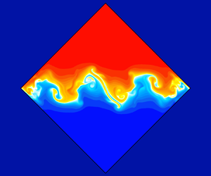Snapshots of the isotherms at various times (denoted by the number of forcing periods, $n_\tau$, following the impulsive start) are shown in figure 8.

Figure 8.

Snapshot of isotherms at the indicated number of forcing periods, $n_\tau$, following an impulsive start to forcing with $\alpha =0.3$ and $\omega =3.6$ at $R_N=10^{5}$. Animations covering a variety of time intervals are shown in supplementary movies 5a to 5e.

Accompanying figure 8 are a number of movies showing temporal evolutions of the isotherms over select intervals. The first of these, supplementary movie 5a, shows the slow ramp-up followed by the initial collapse over $n_\tau \in [30,60]$. Even during the wave-breaking events after $n_\tau \approx 50$, the flow appears to retain centrosymmetry; see the sequence of snapshots from the movie shown in the top two rows of figure 8. However, the asymmetry measure $\mathcal {A}$ grows exponentially until saturating at $n_\tau \approx 170$ (see figure 6e), at which point the asymmetry is visually apparent in the isotherms. The next movie, supplementary movie 5b, covering $n_\tau \in [95,125]$ shows two waves near the horizontal corners being excited while the centre remains relatively static. These break and then a Kelvin–Helmholtz-like roll-up forms at the origin at $n_\tau \approx 115$ (see figure 8). Supplementary movie 5c covers $n_\tau \in [220,240]$. Larger amplitude Faraday wave-like ${\rm L}_2$ oscillations occur at one corner and undergo wave breaking, followed by the formation of sharp undulations that travel horizontally, reminiscent of Holmboe waves. There is also a global sloshing motion, or seiche, with a period of approximately 20 forcing periods, that is most evident in the isotherms away from the central shear region. This period is clearly identifiable in the time series in figure 6(d,e) after 600 forcing periods. In supplementary movie 5d, covering $n_\tau \in [425,455]$, the flow exhibits small-scale cusp-like convective mushrooms travelling towards both horizontal corners. The structures on the hot side of the shear layer travel to the hot corner while those on the cold side travel to the cold corner. Near the end of the animation a roll-up similar to a Kelvin–Helmholtz mushroom appears at the cold corner followed by an ${\rm L}_2$-like excitation of the shear layer. Finally, supplementary movie 5e, covering $n_\tau \in [625,665]$, shows the build-up of Faraday wave-like oscillations that then develop into either left or right travelling waves. As the waves crash into a horizontal corner, there is mixing with the fluid in the interior. The sequence of events in the various movies bears a striking resemblance with the experimental movies of Faraday wave instabilities with miscible fluids in Briard et al. (Reference Briard, Gostiaux and Gréa2020).

5. Summary and conclusions

The responses to vertical parametric modulation of gravity of a fluid in a square container tilted at ${45}^\circ$, with two differentially heated opposite walls and two adiabatic opposite walls, are surprisingly very similar to those from a Faraday wave experiment, in spite of major differences existing in the set-ups. Whereas in the Faraday problem the unforced equilibrium is static, here it is non-trivial, consisting of wall boundary layers and a shear layer centred about the horizontal diagonal separating two near isothermal regions. It is maintained by heat fluxes that are focused near the corners on either side of the shear layer. For sufficiently small forcing amplitudes, there is a forced centrosymmetric synchronous response.

Below a certain viscosity-dependent cutoff forcing frequency, the forced responses have modal cellular structure in the shear layer. Differences in their organization, in particular with respect to parities and symmetries, seem to be connected to the orientation of the forcing. Although gravity is only modulated vertically, the obliqueness of the container walls induces a horizontal component of the forcing whose effects combine with those due to the vertical forcing. The results in Grayer et al. (Reference Grayer, Yalim, Welfert and Lopez2021) indicate that one may expect the non-trivial forced responses at low forcing amplitude to be attributed to this horizontal forcing. Analysis of these different contributions and their interactions will be addressed elsewhere.

Above this cutoff frequency, the forced response is localized at the horizontal corners. Increasing the forcing amplitude at such a frequency leads to parametric subharmonic resonance, much like in the Faraday wave problem. At larger forcing amplitudes, the subharmonic response flow excites a pair of lower frequency modes in a triadic resonance. The identification of such a triadic resonance in a non-uniformly stratified shear flow is novel. Further increases in forcing amplitude lead to low-frequency modulations of the triadic response, resulting in a slow–fast resonant collapse scenario. The slow phase consists of the triadic response growing in amplitude until the response flow in the shear layer interacts with the container walls and, in particular, the horizontal corners. Then, there is a relatively fast collapse and the process repeats. With increasing forcing amplitude, the slow-fast dynamics become more complicated but the flow remains centrosymmetric, with the time-dependent heat fluxes at the hot and cold walls being identical. At much larger forcing amplitude, the response is no longer centrosymmetric, with different heat fluxes at the hot and cold walls. This difference leads to periods of time lasting many forcing periods during which the interior has an excess/deficit of thermal energy, culminating when the Faraday waves with cold/hot fluid encroach on the hot/cold wall as they come crashing near the left/right horizontal corner of the container.

The present configuration provides a relatively simple set-up for generating Faraday waves and studying their instabilities, including triadic resonances and other nonlinear interactions. In particular, it defines a framework for studying the transfer of energy between scales and the effects of shear in non-uniformly stratified flows, which may prove useful in furthering the understanding of these processes in the ocean and the atmosphere.