





1. Introduction
The dynamics of nonlinear waves in plasmas is a classical problem in plasma physics (Akhiezer & Polovin Reference Akhiezer and Polovin1956; Clemmow Reference Clemmow1974; Akhiezer et al. Reference Akhiezer, Akhiezer, Polovin, Sitenko and Stepanov1975). Recently it became important for astrophysical fast radio bursts (FRBs) (Lorimer et al. Reference Lorimer, Bailes, McLaughlin, Narkevic and Crawford2007; Cordes & Chatterjee Reference Cordes and Chatterjee2019; Petroff, Hessels & Lorimer Reference Petroff, Hessels and Lorimer2022). Such FRBs are millisecond-long bursts of radio emission coming from approximately halfway across the Universe. At the peak the (isotropic-equivalent) luminosity (in radio) exceeds billions of solar luminosity (in optical) (Petroff et al. Reference Petroff, Hessels and Lorimer2022).
An important astrophysical hint comes from the observations of correlated radio and X-ray bursts from ultra-magnetised neutron stars (Bochenek et al. Reference Bochenek, Ravi, Belov, Hallinan, Kocz, Kulkarni and McKenna2020; CHIME/FRB Collaboration et al. 2020). This established the FRB–magnetar connection. If the emission originates in the magnetospheres, the laser nonlinearity parameter in these settings can be as high as a staggering
 \begin{equation} a_0 = \frac {e E_w}{m_e c \omega }\sim 10^9, \end{equation}
where $E_w$
is the electric field in the wave and
$E_w$
is the electric field in the wave and $\omega$
is the wave frequency. Parameter regime
$\omega$
is the wave frequency. Parameter regime $a_0 \geqslant 1$
defines relativistic nonlinearity of the wave.
$a_0 \geqslant 1$
defines relativistic nonlinearity of the wave.
In addition, the wave–plasma interaction may occur in the highly magnetised environment, in the regime when the guiding magnetic field strongly affects particle dynamics and laser–plasma interaction. Guide fields can be as strong as, or even exceed, the quantum magnetic field. In addition, plasma parameters are changing as the electromagnetic (EM) pulse propagates away from a neutron star (see e.g. Luan & Goldreich Reference Luan and Goldreich2014; Lyubarsky Reference Lyubarsky2014; Lyutikov, Burzawa & Popov Reference Lyutikov, Burzawa and Popov2016; Beloborodov Reference Beloborodov2021; Lyutikov Reference Lyutikov2021; Golbraikh & Lyubarsky Reference Golbraikh and Lyubarsky2023).
Astrophysical challenges of super-strong waves in plasmas connect to modern laser experiments. The interaction of intense laser beams with plasma is critical for the success of high-energy-density experiments, inertial confinement fusion and, eventually, inertial fusion energy. High-intensity colliding laser pulses also can lead to a new type of laboratory experiments by creating abundant electron–positron pair plasmas (Marklund & Shukla Reference Marklund and Shukla2006; Bell & Kirk Reference Bell and Kirk2008; Ridgers et al. Reference Ridgers, Brady, Duclous, Kirk, Bennett, Arber, Robinson and Bell2012; Zhang et al. Reference Zhang, Bulanov, Seipt, Arefiev and Thomas2020). This process, first discussed more than a decade ago, is becoming a reality.
In addition, for a pair plasma there are a number of principal differences between astrophysical and laboratory set-ups. (i) There are subluminal branches in astrophysical highly magnetised plasmas; waves are relativistically nonlinear. Modern lasers can in principle achieve $a_0 \geqslant 1$
, but usually only in a very limited region of space (extended wave trains typically have
$a_0 \geqslant 1$
, but usually only in a very limited region of space (extended wave trains typically have $a_0 \leqslant 0$
). (ii) Almost universally, in laboratory experiments waves are shone onto a plasma from outside, while in astrophysical settings nonlinear waves can be generated by particles already inside the plasma. These correspond to two different set-ups: boundary condition problem for waves falling from outside, and eigenmode problem for waves inside the plasma.
$a_0 \leqslant 0$
). (ii) Almost universally, in laboratory experiments waves are shone onto a plasma from outside, while in astrophysical settings nonlinear waves can be generated by particles already inside the plasma. These correspond to two different set-ups: boundary condition problem for waves falling from outside, and eigenmode problem for waves inside the plasma.
Finally, there are a number of limitations to numerical particle-in-cell (PIC) approaches. High-intensity EM waves with $a_0 \gg 1$
falling onto a pair plasma accelerate it ponderomotively to relativistic energies, and experiences modulational instability that leads to reflection (Lyutikov & Gurarie Reference Lyutikov and Gurarie2025; Tangtartharakul, Arefiev & Lyutikov Reference Tangtartharakul, Arefiev and Lyutikov2025, these works exploring unmagnetised plasmas). Finally, setting up a subluminal wave already inside a plasma is highly non-trivial in PIC simulations, as all the codes (to the best of our knowledge) ignore the initial current created by the initial particle velocities (initial velocity is not used for current computation until the first update is done). This is especially problematic for subluminal waves, where
$a_0 \gg 1$
falling onto a pair plasma accelerate it ponderomotively to relativistic energies, and experiences modulational instability that leads to reflection (Lyutikov & Gurarie Reference Lyutikov and Gurarie2025; Tangtartharakul, Arefiev & Lyutikov Reference Tangtartharakul, Arefiev and Lyutikov2025, these works exploring unmagnetised plasmas). Finally, setting up a subluminal wave already inside a plasma is highly non-trivial in PIC simulations, as all the codes (to the best of our knowledge) ignore the initial current created by the initial particle velocities (initial velocity is not used for current computation until the first update is done). This is especially problematic for subluminal waves, where $\boldsymbol{\nabla }\times B \sim (4\pi /c) {j}$
. An additional numerical complication of setting nonlinear waves inside a plasma involves the fact that velocity (current), magnetic field and electric field are all evaluated at different times. To set a correct self-consistent nonlinear wave inside a plasma then would involve subtle half-step corrections. These arguments demonstrate the usefulness of a purely theoretical approach.
$\boldsymbol{\nabla }\times B \sim (4\pi /c) {j}$
. An additional numerical complication of setting nonlinear waves inside a plasma involves the fact that velocity (current), magnetic field and electric field are all evaluated at different times. To set a correct self-consistent nonlinear wave inside a plasma then would involve subtle half-step corrections. These arguments demonstrate the usefulness of a purely theoretical approach.
In this paper, we address the basic properties of plasma in this new regime: dispersion relations of relativistically nonlinear waves. We consider a particular case of circularly polarised (CP), fully nonlinear EM waves propagating along a magnetic field. This regime allows, within the two-fluid approximation, a fully nonlinear treatment.
We employ a two-fluid (cold and collisionless) approach. An important advantage of the two-fluid treatment over the magnetohydrodynamics approach (e.g. Heyvaerts, Lehner & Mottez Reference Heyvaerts, Lehner and Mottez2012) is that the current is calculated self-consistently from the dynamic equations for each species.
2. Two-fluid model for relativistically nonlinear CP waves
The governing equations within the two-fluid model for relativistically nonlinear CP waves are exceptionally simple. They include just Maxwell’s equations and transverse force balance:
 \begin{align} \boldsymbol{\nabla }\times \boldsymbol{B} & = {4\pi }\boldsymbol{J}+ \partial _t \boldsymbol{E}, \nonumber \\ \boldsymbol{J} & = e (\boldsymbol{v}_{\kern-1.3pt p} -{\boldsymbol{v}}_{\kern-1pt e}) n ,\nonumber \\ d_t \boldsymbol{p} _{\kern-1pt e,p} & = \mp \left ( \boldsymbol{E} + \frac {\boldsymbol{p} _{e,p}}{\sqrt {1+p_{e,p}^2}} \times \boldsymbol{B} \right )\!, \end{align}
where $ \boldsymbol{p} _{e,p}$
are particle momenta; upper signs are for electrons. Equations are written in the common gyration frame (no axial motion).
$ \boldsymbol{p} _{e,p}$
are particle momenta; upper signs are for electrons. Equations are written in the common gyration frame (no axial motion).
This major simplification comes from the fact that for a fully relativistically nonlinear CP EM wave propagating along a magnetic field (in the $z$
direction), the oscillations are harmonic (this is not true for linearly polarised waves), while density remains constant. This is a major observation underlying the present work.
$z$
direction), the oscillations are harmonic (this is not true for linearly polarised waves), while density remains constant. This is a major observation underlying the present work.
Let us introduce a unit vector corresponding to the wave vector potential:
 \begin{equation} \boldsymbol{e} _w= \left \{\cos ( \omega t- k z),-\sin (\omega t- k z),0\right \}\!. \end{equation}
The motion of particles in the EM field (guide plus waves) consists of forced motion by the wave and free oscillations. Importantly, we are interested in forced oscillations due to the influence of the wave on particle motion. (Though this statement seems obvious, it is an important point in selecting the correct dispersion branches; see § 5.3.) In this case, for CP waves, the momentum of the particles is parallel to the wave magnetic field (aligned or counter-aligned). Thus we can write
 \begin{equation} \boldsymbol{p} _{e,p} = a _{e,p} \boldsymbol{e} _w .\end{equation}
The relations (2.1) then give
 \begin{align} & n^2-1= \left (\frac {a_{\kern-0.7pt p}}{\sqrt {1+ a_p^2}}-\frac {a_e}{\sqrt {1+ a_e^2}}\right ) \frac {\omega _p^2 }{ a_0 \omega ^2} = (\tanh\!\,\chi _p-\tanh\!\,\chi _e)\, \frac {\omega _p^2 }{a_0 \omega ^2},\\[-8pt]\nonumber \end{align}
 \begin{align} & {a_0}= \left ( \frac {f_B}{\sqrt {1+ a_p^2}}-1 \right ) a_{\kern-0.7pt p} =\tanh\!\,\chi _p (f_B-\cosh \chi _p),\\[-8pt]\nonumber \end{align}
 \begin{align} & {a_0}= \left ( \frac {f_B}{\sqrt {1+ a_e^2}}+1 \right ) a_e =\tanh\!\, \chi _e (f_B+\cosh \chi _e),\\[-8pt]\nonumber \end{align}
 \begin{align} & a_{p,e} \equiv \sinh (\chi _{e,p} ), \end{align}
where $n=k/\omega$
, frequency parameter
$n=k/\omega$
, frequency parameter $ f_B = {\omega _B}/{\omega }$
and we introduced rapidity
$ f_B = {\omega _B}/{\omega }$
and we introduced rapidity $\chi _{e,p}$
(so that
$\chi _{e,p}$
(so that $v_{e,p} = \tanh (\chi _{e,p} )$
).
$v_{e,p} = \tanh (\chi _{e,p} )$
).
In (2.7) the plasma frequency
 \begin{equation} \omega _p^2 = \frac {4 \pi e^2 n}{m_e} \end{equation}
is defined with respect to the density of each component (e.g. in pair plasma the relevant terms in the dispersion relations are $ \propto 2 \omega _p^2$
). The cyclotron frequency
$ \propto 2 \omega _p^2$
). The cyclotron frequency
 \begin{equation} \omega _B = \frac {e B}{m_e c} \end{equation}
is positively defined; the signs of charges are explicitly taken into account.
In what follows, whenever dimensionless momentum or energy appear, they should be understood in terms of $p/(m_e c)$
and
$p/(m_e c)$
and $\epsilon /(m_e c^2)$
. The speed of light and elementary charge are set to unity. When we refer to the electron–ion case (e–i), the ions are assumed to be motionless (
$\epsilon /(m_e c^2)$
. The speed of light and elementary charge are set to unity. When we refer to the electron–ion case (e–i), the ions are assumed to be motionless ( $m_i \to \infty$
limit). To keep the notations consistent, electron quantities come with a subscript
$m_i \to \infty$
limit). To keep the notations consistent, electron quantities come with a subscript $e$
, while ion and positron quantities come with a subscript
$e$
, while ion and positron quantities come with a subscript $p$
.
$p$
.
By our choice of polarisation and direction of magnetic field, quantity $a_e$
is always positive, while
$a_e$
is always positive, while $a_{\kern-0.5pt p}$
can have either sign. This is related to the possibility of cyclotron resonance: by the choice of polarisation, it is the positively charged particles (positrons) that can be in resonance. Below we refer to them as ‘resonant particles’ – this term is related to the type of particles, not particular particles that are in resonance.
$a_{\kern-0.5pt p}$
can have either sign. This is related to the possibility of cyclotron resonance: by the choice of polarisation, it is the positively charged particles (positrons) that can be in resonance. Below we refer to them as ‘resonant particles’ – this term is related to the type of particles, not particular particles that are in resonance.
Given our choice of polarisation, $|\chi _p| \gt \chi _e$
. Thus, superluminal waves correspond to
$|\chi _p| \gt \chi _e$
. Thus, superluminal waves correspond to $\chi _p \lt 0$
, while subluminal waves correspond to
$\chi _p \lt 0$
, while subluminal waves correspond to $\chi _p \gt 0$
.
$\chi _p \gt 0$
.
3. Basic linear plasma waves propagating along magnetic field
As we are interested in relativistic modifications, let us briefly review the conventional linear case (e.g. Akhiezer et al. Reference Akhiezer, Akhiezer, Polovin, Sitenko and Stepanov1975), see figure 1, in which case fluctuating quantities and dispersion relation are
 \begin{align} v_{0,e} & = a_0 \frac {\omega }{\omega +\omega _B}, \nonumber \\[3pt] v_{0,p} & = a_0 \frac {\omega }{\omega _B- \omega }, \nonumber \\[3pt] |v_{0,p}| & \gt v_{0,e}, \nonumber \\[3pt] r_p & = \frac {|v_{0,p}| }{\omega } \gt r_e = \frac {|v_{0,e}| }{\omega }, \nonumber \\[3pt] n^2 -1 & = - \left ( \frac {1}{\omega \left (\omega _B-\omega \right )} + \frac {1}{\omega \left (\omega _B+\omega \right )}\right ) \omega _p^2 \overset {\mathrm{pairs}}{\to } \frac {2 \omega _p^2}{\omega _B^2-\omega ^2 } ,\end{align}
where $r_{e,p}$
are corresponding Larmor radii. In (3.1), we explicitly separated contributions from resonant and non-resonant particles. The final expression, after
$r_{e,p}$
are corresponding Larmor radii. In (3.1), we explicitly separated contributions from resonant and non-resonant particles. The final expression, after $\to$
sign, is for a pair plasma. Notice that at
$\to$
sign, is for a pair plasma. Notice that at $\omega \gt \omega _B$
velocities of particles are counter-aligned with respect to each other, so that their currents add, while for
$\omega \gt \omega _B$
velocities of particles are counter-aligned with respect to each other, so that their currents add, while for $\omega \lt \omega _B$
velocities of particles are aligned so that their currents subtract. For definiteness, we label the direction of rotation with respect to non-resonant particles, so that ‘co-rotating resonant particles’ means the velocities of two species are aligned (in the linear case, this occurs for
$\omega \lt \omega _B$
velocities of particles are aligned so that their currents subtract. For definiteness, we label the direction of rotation with respect to non-resonant particles, so that ‘co-rotating resonant particles’ means the velocities of two species are aligned (in the linear case, this occurs for $\omega _B \gt \omega$
; see (3.1)).
$\omega _B \gt \omega$
; see (3.1)).
The subluminal branches, whistler and/or Alfvén, extend to $0\lt \omega \lt \omega _B$
. At small
$0\lt \omega \lt \omega _B$
. At small $\omega \ll \omega _B$
,
$\omega \ll \omega _B$
,
 \begin{eqnarray} & \omega = \dfrac {k^2 \omega _B}{\omega _p^2}, & \quad \text{whistlers}, \nonumber \\ & \dfrac {k^2}{\omega ^2} = 1+ \dfrac {2 \omega _p^2}{\omega _B^2} = 1+ \dfrac {2}{\sigma } , & \quad \text{Alfv}\acute{\text{e}}\text{n}, \end{eqnarray}
where
 \begin{equation} \sigma =\frac {\omega _B^2}{\omega _p^2} \end{equation}
is the magnetisation parameter (Kennel & Coroniti Reference Kennel and Coroniti1984).
Superluminal branches have a cutoff at
 \begin{eqnarray} & \omega _{\mathrm{uh}}= \sqrt {\omega _B^2 + 2 \omega _p^2} = \sqrt {2+\sigma } \omega _p, & \ \text{pairs, upper hybrid frequency}, \nonumber \\[4pt] & \omega =\dfrac {1}{2} \left (\dfrac {\omega _B}{\omega _p}+\sqrt {4+ \dfrac {\omega _B^2}{\omega _p^2}}\right ) = \dfrac {1}{2} ( \sqrt {4+\sigma } + \sqrt {\sigma } ) \omega _p , & \ \text{resonant EM branch}, \nonumber \\[4pt] & \omega = \dfrac {1}{2} \left (\sqrt {4+ \dfrac {\omega _B^2}{\omega _p^2}}- \dfrac {\omega _B}{\omega _p}\right ) = \dfrac {1}{2} ( \sqrt {4+\sigma } - \sqrt {\sigma } ) \omega _p, & \ \text{non-resonant EM branch}. \end{eqnarray}
Dispersion relations for linear waves for particular choice $ \sigma \equiv (\omega _B/\omega _p)^2=1$
.
$ \sigma \equiv (\omega _B/\omega _p)^2=1$
.

Figure 1 Long description
A line graph showing dispersion relations for linear waves with a specific choice of sigma equal to 1. The horizontal axis represents the wave number k divided by the plasma frequency omega p, ranging from 0 to 2. The vertical axis represents the frequency omega divided by the plasma frequency omega p, ranging from 0 to 2. The graph includes multiple lines representing different branches and conditions. The red lines indicate the pairs (EM branch) and pairs (Alfven branch), while the blue dashed lines represent the resonant (EM branch) and resonant (whistler branch). Key annotations include labels for different branches, gaps for pairs and resonant conditions, and specific mathematical expressions related to the wave properties. The graph illustrates how the dispersion relations vary under different conditions, highlighting the effects of wave intensity and magnetic field on the propagation of waves.
Various particles’ trajectories and forces are sketched in figure 2 (equal masses are assumed). There are two forces acting on a particle: electric field of the wave $E_w$
and the Lorentz force from the guide field
$E_w$
and the Lorentz force from the guide field $v_{e,p} B_0$
. For non-resonant particles, both forces add. For resonant particles they subtract: for
$v_{e,p} B_0$
. For non-resonant particles, both forces add. For resonant particles they subtract: for $\omega \gt \omega _B$
the force from the electric field is larger, while for
$\omega \gt \omega _B$
the force from the electric field is larger, while for $\omega \lt \omega _B$
the Lorentz force dominates.
$\omega \lt \omega _B$
the Lorentz force dominates.
Particle trajectories in CP EM waves propagating along the magnetic field. Top left: in external magnetic field without the wave; top right: in EM wave without guide magnetic field. In both cases at each point velocities of oppositely charged particles are counter-aligned (so the currents add). Bottom row shows trajectories in magnetic field. Left: weak magnetic field (velocities counter-aligned, currents add); right: strong magnetic field (velocities aligned, currents subtract).

4. Single-particle motion in nonlinear CP EM wave with guide field
For the CP wave, the dispersion relations and force balance equations separate. This allows fully nonlinear treatment. We first consider single-particle dynamics in the presence of a CP wave and guide magnetic field (propagation along the field). For now, the frequency of the wave $\omega$
is considered as given. In plasma, § 5, the wave frequency in the gyration frame has to be calculated self-consistently.
$\omega$
is considered as given. In plasma, § 5, the wave frequency in the gyration frame has to be calculated self-consistently.
A special type of solution (not a general one starting with arbitrary initial conditions) involves particle velocities instantaneously (counter-)aligned with the wave’s magnetic field. The force balance can be written in a fairly compact form:
 \begin{equation} \gamma _\pm m_e v _\pm \omega = e ( E_w \pm v _\pm B_0), \end{equation}
where $ \pm$
accounts for two directions of the background field/charge/polarisation sign (speed of light is set to unity). But different realisations are fairly complicated depending on the values of the wave electric field, guide
$ \pm$
accounts for two directions of the background field/charge/polarisation sign (speed of light is set to unity). But different realisations are fairly complicated depending on the values of the wave electric field, guide $B_0$
and wave frequency
$B_0$
and wave frequency $\omega$
. They are illustrated in figure 2.
$\omega$
. They are illustrated in figure 2.
Particle momenta in nonlinear CP waves. For $ \omega \geqslant \omega _B$
(
$ \omega \geqslant \omega _B$
( $f_B= \omega _B/\omega \geqslant 1$
, including the case
$f_B= \omega _B/\omega \geqslant 1$
, including the case $\omega =\omega _B$
), resonant particles are counter-rotating (negative
$\omega =\omega _B$
), resonant particles are counter-rotating (negative $\chi _p$
). For
$\chi _p$
). For $ \omega \lt \omega _B$
, resonant particles are co-rotating for mild
$ \omega \lt \omega _B$
, resonant particles are co-rotating for mild $a_0\leqslant (f_B^{2/3}-1)^{3/2}$
and counter-rotating for larger
$a_0\leqslant (f_B^{2/3}-1)^{3/2}$
and counter-rotating for larger $a_0$
. Dashed branches are likely to be unstable.
$a_0$
. Dashed branches are likely to be unstable.

Momenta of non-resonant $a_e$
(dot–dashed lines in figure 3) are positive
$a_e$
(dot–dashed lines in figure 3) are positive $a_e\gt 0$
by our choice of polarisation. Dependence of
$a_e\gt 0$
by our choice of polarisation. Dependence of $a_e$
on parameters is fairly straightforward.
$a_e$
on parameters is fairly straightforward.
The most interesting case is for particles that may be in resonance. (Recall that, in the linear case, $ a_0 = a_{\kern-0.5pt p} (f_B -1)$
, the resonance is reached at
$ a_0 = a_{\kern-0.5pt p} (f_B -1)$
, the resonance is reached at $f_B=1$
. Below the resonance
$f_B=1$
. Below the resonance $a_{\kern-0.5pt p}\lt 0$
(counter-aligned with non-resonant particles), while above the resonance
$a_{\kern-0.5pt p}\lt 0$
(counter-aligned with non-resonant particles), while above the resonance $a_{\kern-0.5pt p}\gt 0$
(aligned).)
$a_{\kern-0.5pt p}\gt 0$
(aligned).)
Nonlinear effects make the most important modifications for particle trajectories near the resonance $f_B \approx 1$
. Formally, the resonance shifts from
$f_B \approx 1$
. Formally, the resonance shifts from $f_B=1$
to
$f_B=1$
to
 \begin{equation} a_{\kern-0.7pt p} = \sqrt {f_B^2-1}. \end{equation}
But, in fact, it is never reached, as we discuss next.
First, consider a special case $f_B=1$
(thick line in figure 3). In this case, momentum is determined from
$f_B=1$
(thick line in figure 3). In this case, momentum is determined from
 \begin{equation} a_0= \tanh (\chi _p )-\sinh (\chi _p).\end{equation}
This is an equation for $\chi _p(a_0)$
. Since
$\chi _p(a_0)$
. Since $a_0 \gt 0$
by definition, negative
$a_0 \gt 0$
by definition, negative $\chi _p$
is needed (resonant particles are still counter-aligned with non-resonant particles, just like for
$\chi _p$
is needed (resonant particles are still counter-aligned with non-resonant particles, just like for $f_B \lt 1$
).
$f_B \lt 1$
).
For small $a_0$
,
$a_0$
,
 \begin{equation} a_{\kern-0.7pt p} = - (2 a_0)^{1/3}. \end{equation}
Thus, for the special case $f_B=1$
particle motion is not a linear response to wave intensity in the small
$f_B=1$
particle motion is not a linear response to wave intensity in the small $a_0\ll 1$
limit. For any
$a_0\ll 1$
limit. For any $f_B \neq 1$
, the response is linear,
$f_B \neq 1$
, the response is linear, $ |a_{\kern-0.5pt p}| \propto a_0$
in the limit
$ |a_{\kern-0.5pt p}| \propto a_0$
in the limit $a_0 \to 0$
.
$a_0 \to 0$
.
The situation slightly above the resonance, $f_B \geqslant 1$
, is more complicated:
$f_B \geqslant 1$
, is more complicated:
-
(i) At mild intensities, $a_0 \leqslant a_0^{(\mathrm{crit})}= (f_B^{2/3} -1)^{3/2}$
, there are three branches for the solution
$a_{\kern-0.5pt p} (a_0)$
. The physical one (least energy of a particle and correct limit for
$a_0 \to 0$
) is co-rotating – positive
$\chi _p$
(thick curve in figure 3, near
$f_B=2$
box). Thus, the synchrotron resonance (4.2) is located on the upper curve, and hence is never reached. (We encounter here a mathematical oddity: a formal solution for forced oscillations
$a_{\kern-0.5pt p}(a_0)$
connects to free oscillations
$\omega = \omega _B/\gamma _p$
at
$a_0 =0$
.) The nonlinear cyclotron resonance (4.2) corresponds to particles gyrating without a wave. Hence, this point does not reflect a response of plasma to an EM perturbation – it is an initial condition on particle velocities.
$a_0 \leqslant a_0^{(\mathrm{crit})}= (f_B^{2/3} -1)^{3/2}$
, there are three branches for the solution
$a_{\kern-0.5pt p} (a_0)$
. The physical one (least energy of a particle and correct limit for
$a_0 \to 0$
) is co-rotating – positive
$\chi _p$
(thick curve in figure 3, near
$f_B=2$
box). Thus, the synchrotron resonance (4.2) is located on the upper curve, and hence is never reached. (We encounter here a mathematical oddity: a formal solution for forced oscillations
$a_{\kern-0.5pt p}(a_0)$
connects to free oscillations
$\omega = \omega _B/\gamma _p$
at
$a_0 =0$
.) The nonlinear cyclotron resonance (4.2) corresponds to particles gyrating without a wave. Hence, this point does not reflect a response of plasma to an EM perturbation – it is an initial condition on particle velocities. -
(ii) At intensities
$a_0 \geqslant a_0^{(\mathrm{crit})}$
there is only one counter-rotating branch (solid curve at bottom right in figure 3). Thus, for fixed
$f_B\gt 1$
(below cyclotron resonance) and increasing
$a_0$
there is a transition (indicated by a vertical arrow) from a co-rotating to a counter-rotating state. Since counter-rotating states correspond to superluminal waves, for a given
$a_0$
there are no subluminal waves beyond some
$k$
.



5. Relativistically nonlinear CP EM waves in magnetised plasma
Next, we finally turn to the properties of nonlinear EM waves in a pair plasma. Above, in § 4, we considered frequency as given. It is, in fact, determined by the properties of the plasma.
An additional complication comes from the arbitrary dependence of wave intensity on frequency: $a_0(\omega )$
is a free parameter. Generally, the dispersion relation has the form
$a_0(\omega )$
is a free parameter. Generally, the dispersion relation has the form
 \begin{equation} \omega = \omega ( k, a_0(\omega )). \end{equation}
Various $a_0(\omega )$
will produce different dispersions
$a_0(\omega )$
will produce different dispersions $\omega (k)$
.
$\omega (k)$
.
Nonlinear cutoff frequencies, as a ratio to linear ones, (3.4). In all cases, cutoff frequencies decrease with large $a_0$
.
$a_0$
.

In what follows, we first consider an exemplary case of constant $a_0(\omega )$
. It highlights the key point: relativistically nonlinear subluminal modes terminate at some
$a_0(\omega )$
. It highlights the key point: relativistically nonlinear subluminal modes terminate at some $\omega ^\ast {-}k^\ast$
point on the
$\omega ^\ast {-}k^\ast$
point on the $\omega {-}k$
plane. Later, in § 5.4, we highlight general relations and discuss the case of constant ratio
$\omega {-}k$
plane. Later, in § 5.4, we highlight general relations and discuss the case of constant ratio $E_w/B_0$
(wave intensity to guide field).
$E_w/B_0$
(wave intensity to guide field).
The cases of single components and pair plasma are somewhat different. For the single-component case, the mathematics is simpler: eliminate particle momenta from the force balance, and use it in the expression for $n^2-1$
. In a pair plasma, the procedure is more complicated: particle momenta
$n^2-1$
. In a pair plasma, the procedure is more complicated: particle momenta $a_{e,p}$
both depend on the resulting wave frequency.
$a_{e,p}$
both depend on the resulting wave frequency.
5.1. Superluminal modes
Superluminal modes have $\chi _p \lt 0$
. All superluminal modes (R, L and Alfvén) have cutoffs at (figure 4)
$\chi _p \lt 0$
. All superluminal modes (R, L and Alfvén) have cutoffs at (figure 4)
 \begin{equation} \omega _{\mathrm{cut}} ^2 = \frac {\tanh\!\,\chi _e-\tanh\!\,\chi _p}{a_0} \omega _p^2. \end{equation}
For the single-component cases, these relations can be resolved analytically. The resonant ( $\chi _p \lt 0$
) case is
$\chi _p \lt 0$
) case is
 \begin{eqnarray} && \omega _{\mathrm{cut}} ^2 = \frac {\tanh |\chi _{p}|)}{a_0} \omega _p^2 = \frac {\omega _p^2}{\cosh (\chi _p)-f_B}=\frac {1}{2} \text{sech}(\chi _p) \left (\sqrt {\omega _B^2+4 \omega _p^2 \cosh (\chi _p)}+\omega _B\right )\!, \nonumber \\ && a_0=f_B \tanh (\chi _p)-\sinh (\chi _p) = \sinh (\chi _p) \left (\frac {2 \omega _B}{\sqrt {\omega _B^2+4 \omega _p^2 \cosh (\chi _p)}+\omega _B}-1\right )\!. \end{eqnarray}
The non-resonant case is
 \begin{align} \omega _{\mathrm{cut}} ^2 & = \frac {\tanh\!\,\chi _{e}}{a_0} \omega _p^2 = \frac {\omega _p^2}{\cosh \left (\chi _ e\right )+f_B}=\frac {1}{2} \text{sech}\left (\chi _e\right ) \left (\sqrt {\omega _B^2+4 \omega _p^2 \cosh \left (\chi _e\right )}-\omega _B\right )\!, \nonumber \\[7pt] a_0 & =f_B \tanh \left (\chi _e\right )+\sinh \left (\chi _e\right ) \nonumber \\[7pt] & =\frac {\omega _B \tanh \left (\chi _e\right ) \left (\sqrt {\omega _B^2+4 \omega _p^2 \cosh \left (\chi _e\right )}+\omega _B\right )}{2 \omega _p^2}+\sinh \left (\chi _e\right ) \end{align}
(compare with (8.1.4.2) in Akhiezer et al. (Reference Akhiezer, Akhiezer, Polovin, Sitenko and Stepanov1975)).
For a pair plasma, the cutoff frequencies cannot be put into a compact expression. A good approximation is achieved if we use
 \begin{eqnarray} && \omega _B \to \omega _B / \big( 1+a_0^{2/3}\big)^{3/2}, \nonumber \\[3pt] && \omega _p \to \omega _p/\big(1+a_0^2\big)^{1/4} \end{eqnarray}
(see figure 5). The relation for $\omega _p$
is exact for the
$\omega _p$
is exact for the $\omega _B=0$
case (Akhiezer & Polovin Reference Akhiezer and Polovin1956).
$\omega _B=0$
case (Akhiezer & Polovin Reference Akhiezer and Polovin1956).


In figure 6, we plot dispersion curves for superluminal modes. Qualitatively, the curves look similar to those of the linear case, with cutoff frequencies shifted down for large $a_0$
.
$a_0$
.
Dispersion curves for superluminal modes for $\sigma =1$
,
$\sigma =1$
, $a_0 =0.1,\ 1,\ 10$
(top to bottom).
$a_0 =0.1,\ 1,\ 10$
(top to bottom).

5.2. Subluminal modes
There are two types of subluminal modes: whistler (single-component, resonant) and Alfvén (pairs) modes; there are no subluminal modes corresponding to single-component non-resonant particles.
A qualitatively new effect appears for subluminal modes – bend of the dispersion relation at finite $\omega ^\ast {-}k^\ast$
(figure 7). At the bend, the group velocity
$\omega ^\ast {-}k^\ast$
(figure 7). At the bend, the group velocity $v_g = \partial \omega / \partial k$
becomes zero. Above the bend (at higher
$v_g = \partial \omega / \partial k$
becomes zero. Above the bend (at higher $k$
), the group velocity is negative.
$k$
), the group velocity is negative.
Dispersion curves for relativistically nonlinear whistler (left panel) and Alfvén (right panel) waves, $\sigma =1$
. Dispersion curves experience a bend at finite
$\sigma =1$
. Dispersion curves experience a bend at finite $k^\ast {-} \omega ^\ast$
; above this point, resonant particles are on the upper branch in figure 3. Dispersion curves terminate at
$k^\ast {-} \omega ^\ast$
; above this point, resonant particles are on the upper branch in figure 3. Dispersion curves terminate at $\omega =0$
,
$\omega =0$
, $k_{\mathrm{max}} = \omega _p/\sqrt {a_0}$
(lower row of points).
$k_{\mathrm{max}} = \omega _p/\sqrt {a_0}$
(lower row of points).

Recall that subluminal modes correspond to $f_B \geqslant 1$
, while the resonant component has
$f_B \geqslant 1$
, while the resonant component has $\chi _p \geqslant 0$
. With increasing
$\chi _p \geqslant 0$
. With increasing $a_0$
it follows the middle branch in figure 3. The middle branch
$a_0$
it follows the middle branch in figure 3. The middle branch $a_{\kern-0.5pt p} (a_0)$
terminates at some finite
$a_{\kern-0.5pt p} (a_0)$
terminates at some finite $a_0$
. The critical point corresponds to
$a_0$
. The critical point corresponds to
 \begin{equation} \omega ^\ast = \frac {\omega _B}{\big(1+ a_0^{2/3}\big){}^{3/2}} \to \frac {\omega _B}{a_0} \end{equation}
(the latter relation is for $a_0 \gg 1$
). It is the same for both whistler and Alfvén modes.
$a_0 \gg 1$
). It is the same for both whistler and Alfvén modes.
For fixed $a_0(\omega )=$
const., dispersion curves bend over in the
$a_0(\omega )=$
const., dispersion curves bend over in the $\omega {-}k$
plane at some finite values of
$\omega {-}k$
plane at some finite values of $\omega ^\ast {-}k^\ast$
, and since above the bend modes are likely to be unstable, the dispersion curve effectively terminates. At frequencies well below the cyclotron frequency,
$\omega ^\ast {-}k^\ast$
, and since above the bend modes are likely to be unstable, the dispersion curve effectively terminates. At frequencies well below the cyclotron frequency, $f_B \gg 1$
, Alfvén waves exist only for
$f_B \gg 1$
, Alfvén waves exist only for $\omega \leqslant \omega _B/ a_0$
, or reverting to the fields,
$\omega \leqslant \omega _B/ a_0$
, or reverting to the fields,
 \begin{align} E_w \leqslant B_0 \end{align}
(see § 5.4).
For single-component plasma (relativistically nonlinear whistler modes), the corresponding wave vector and phase velocities are
 \begin{align} k^2 & = \omega ^2-\frac {\omega \omega _p^2}{\omega \sqrt {1+ a_p^2}-\omega _B}, \nonumber \\[4pt] k^{\ast , 2} & = \frac {\omega _B^2}{\big(1+a_0^{2/3}\big){}^3}+\frac {\omega _p^2}{\sqrt {1+a_0^{2/3}} a_0^{2/3}}, \nonumber \\[4pt] v ^{\ast , 2} & = \frac {a_0^{2/3} \sigma }{a_0^{2/3} \sigma +\big(1+ a_0^{2/3}\big){}^{5/2}} \to \frac {\sigma }{a_0 + \sigma }, \end{align}
where $ v ^\ast$
is the terminal phase velocity of whistler modes (figure 7, left panel).
$ v ^\ast$
is the terminal phase velocity of whistler modes (figure 7, left panel).
For relativistic whistler modes, the maximal phase velocity is reached at
 \begin{align} a_0 & = (2/3)^{3/2} = 0.544, \nonumber \\[6pt] v ^{\ast }_{\textrm {max}} & = \sqrt {\frac {\sigma }{\sigma +{25 \sqrt {({5}/{3})}}/{6}}}, \nonumber \\[6pt] \gamma ^{\ast , 2} & =1+ \frac {6}{25} \sqrt {\frac {3}{5}} \sigma .\end{align}
The dispersion curve ends at $\omega =0$
,
$\omega =0$
, $k_{max}=\omega _p/\sqrt {\alpha _0}$
(lower row of points in figure 7).
$k_{max}=\omega _p/\sqrt {\alpha _0}$
(lower row of points in figure 7).
In a pair plasma $ k^{\ast }$
(terminal wave vector for relativistically nonlinear Alfvén waves) has to be found numerically (figure 7, right panel).
$ k^{\ast }$
(terminal wave vector for relativistically nonlinear Alfvén waves) has to be found numerically (figure 7, right panel).
In figure 8 we plot terminal Alfvén velocities as a function of $a_0$
for different magnetisations. For comparison, in dashed lines we show linear Alfvén speed for
$a_0$
for different magnetisations. For comparison, in dashed lines we show linear Alfvén speed for $\omega \to 0$
,
$\omega \to 0$
, $v_A = \sqrt {{\sigma }/({2+ \sigma })}$
(the factor
$v_A = \sqrt {{\sigma }/({2+ \sigma })}$
(the factor $2$
accounts for two species;
$2$
accounts for two species; $\sigma$
is defined with respect to each separately). Relativistically nonlinear Alfvén waves are slower due to increasing effective mass.
$\sigma$
is defined with respect to each separately). Relativistically nonlinear Alfvén waves are slower due to increasing effective mass.
Terminal phase velocities for Alfvén waves, $\sigma =1$
. Dashed lines are linear limits for
$\sigma =1$
. Dashed lines are linear limits for $k\to 0$
,
$k\to 0$
, $v_A = \sqrt {{\sigma }/({2+ \sigma })}$
.
$v_A = \sqrt {{\sigma }/({2+ \sigma })}$
.

5.3. Negative group velocity branch and the bend in
$\omega (k)$

Negative group velocity branches, at $k\gt k^\ast$
, are likely to be unstable. The stability criterion for linear waves (Landau & Lifshitz Reference Landau and Lifshitz1960, pp. 80 and 84) is violated:
$k\gt k^\ast$
, are likely to be unstable. The stability criterion for linear waves (Landau & Lifshitz Reference Landau and Lifshitz1960, pp. 80 and 84) is violated:
 \begin{align} \partial _\omega (\omega \epsilon (\omega )) = - n^2 - 2 n (\partial _k \omega )^{-1} \lt 0. \end{align}
This indicates that the wave has negative energy and is likely to become unstable by coupling to the positive energy modes. Negative energy of the wave indicates that the wave would take energy from the plasma components.
As figure 3 indicates, at any given $a_0$
, the upper branch has particles with larger momenta than the lower branch. It is an interesting coincidence that dispersion curves, which describe the response of a medium to a perturbation, terminate at free-rotating particles.
$a_0$
, the upper branch has particles with larger momenta than the lower branch. It is an interesting coincidence that dispersion curves, which describe the response of a medium to a perturbation, terminate at free-rotating particles.
As another argument in favour of instability of a branch above $k\gt k^\ast$
, the terminal point
$k\gt k^\ast$
, the terminal point $\omega =0, \, k \neq 0$
corresponds to the conditions for electron cyclotron maser/gyrotron instability (Melrose Reference Melrose1989), with the exception that in a pair plasma both components have distribution in perpendicular momenta
$\omega =0, \, k \neq 0$
corresponds to the conditions for electron cyclotron maser/gyrotron instability (Melrose Reference Melrose1989), with the exception that in a pair plasma both components have distribution in perpendicular momenta $\propto \delta ( a_{e/p} - p_{0, e/p})$
. This clearly indicates population inversion and instability. Finally, negative group velocity is possible in media with inverted populations, and hence unstable (Garrett & McCumber Reference Garrett and McCumber1970).
$\propto \delta ( a_{e/p} - p_{0, e/p})$
. This clearly indicates population inversion and instability. Finally, negative group velocity is possible in media with inverted populations, and hence unstable (Garrett & McCumber Reference Garrett and McCumber1970).
In passing, we note that there are in fact media where the phase and group velocities of EM waves are oppositely directed: they go under the name left-handed media or negative-index metamaterials (Veselago Reference Veselago1968). The difference is that experimental set-ups with $n\lt 0$
are fixed, while here they are dynamic. Another prominent case when phase and group velocities are counter-aligned is the Cherenkov emission (e.g. Bolotovskii & Stolyarov Reference Bolotovskii and Stolyarov1975).
$n\lt 0$
are fixed, while here they are dynamic. Another prominent case when phase and group velocities are counter-aligned is the Cherenkov emission (e.g. Bolotovskii & Stolyarov Reference Bolotovskii and Stolyarov1975).
5.4. Dispersion relations for arbitrary
$\eta _w = E_w/B_0$

Above, we considered a case of constant $a_0(\omega ) \equiv a_0$
, and hence increasing wave electric field
$a_0(\omega ) \equiv a_0$
, and hence increasing wave electric field $E_w(\omega ) \propto \omega$
. We found that Alfvén wave dispersion terminates at
$E_w(\omega ) \propto \omega$
. We found that Alfvén wave dispersion terminates at $E_w \sim B_0$
. Next, we discuss generation properties of the dispersion relation, and repeat calculations for arbitrary
$E_w \sim B_0$
. Next, we discuss generation properties of the dispersion relation, and repeat calculations for arbitrary $\eta _w = E_w/B_0$
.
$\eta _w = E_w/B_0$
.
Same a figure 7, assuming constant ratio of wave intensity to guide field $\eta _w = E_w/B_0$
.
$\eta _w = E_w/B_0$
.

Instead of (2.7), for given $\eta _w$
we find
$\eta _w$
we find
 \begin{align} n^2-1 & = \left (\frac {a_{\kern-0.5pt p}}{\sqrt {1+ a_p^2}}-\frac {a_e}{\sqrt {1+ a_e^2}}\right ) \frac {1}{\eta _w} \frac {\omega _p^2}{\omega \omega _B} = \big(\!\tanh\!\,\chi _p-\tanh\!\,\chi _e\big)\, \frac {1}{\eta _w} \frac {\omega _p^2}{\omega \omega _B} ,\nonumber \\ \eta _w & = \left (\frac {1}{\sqrt {1+a_p^2}}-\frac {\omega }{\omega _B}\right ) a_{\kern-0.5pt p} =\tanh\!\,\chi _p - \frac {\sinh \chi _p}{f_B}, \nonumber \\ \eta _w & = \left (\frac {1}{\sqrt {1+a_e^2}}+\frac {\omega }{\omega _B}\right ) a_e =\tanh\!\,\chi _e + \frac {\sinh \chi _e}{f_B}. \end{align}
For frequency-dependent $\eta _w(\omega )$
, the relation (5.6) for the critical frequency, where dispersion of subluminal modes terminates, can be written as
$\eta _w(\omega )$
, the relation (5.6) for the critical frequency, where dispersion of subluminal modes terminates, can be written as
 \begin{align} \tilde {\omega }^{\ast } & = \frac { \omega ^\ast }{ \omega _B}= \left (1 - \left ( \eta _w \right ) ^{2/3} \right ) ^{3/2}, \nonumber \\ a_p^\ast & = \sqrt {\frac {1}{ \tilde {\omega }^{\ast , 2/3}}-1} = \frac { \eta _w^{1/3}}{\sqrt {1-\eta _w^2}}, \nonumber \\ \eta _w (\omega ) & = \frac { E_w(\omega ) }{B_0}. \end{align}
In figure 9 we plot the dispersion curves for relativistically nonlinear subluminal waves assuming a constant ratio of wave intensity to guide field $\eta _w = E_w/B_0$
. With increasing
$\eta _w = E_w/B_0$
. With increasing $\eta _w$
, propagating waves are confined to smaller corner near
$\eta _w$
, propagating waves are confined to smaller corner near $\omega ,\, k \approx 0$
. For
$\omega ,\, k \approx 0$
. For $\eta _w \geqslant 1$
waves cannot propagate.
$\eta _w \geqslant 1$
waves cannot propagate.
Relation (5.12) highlights the universal relationship: when at a given frequency the intensity of the fluctuating field in a subluminal wave exceeds the guide field, $\eta _w \to 1$
, the wave cannot propagate.
$\eta _w \to 1$
, the wave cannot propagate.
5.5. Finite ion mass
In the case of finite mass of the ion component, $\mu = m_p/m_e \neq 1, \infty$
, general relations are much more complicated, as two new frequencies appear (ion cyclotron and ion plasma), both modified by the nonlinear effects. To achieve relativistic motion of ions in unmagnetised plasma, a wave should be
$\mu = m_p/m_e \neq 1, \infty$
, general relations are much more complicated, as two new frequencies appear (ion cyclotron and ion plasma), both modified by the nonlinear effects. To achieve relativistic motion of ions in unmagnetised plasma, a wave should be $ a_0 \sim \mu = 1836$
(
$ a_0 \sim \mu = 1836$
( $a_0$
is defined with respect to the electron mass).
$a_0$
is defined with respect to the electron mass).
Introduction of a guide field leads to a number of complications. Here the form (5.11) provides a better insight. First, the equation for plasma response involves $\omega _p^2/\omega _B$
and is thus mass-independent. Mass dependence enters through dynamical equations for velocities of the two components.
$\omega _p^2/\omega _B$
and is thus mass-independent. Mass dependence enters through dynamical equations for velocities of the two components.
As we discussed above, the most important point is the fairly subtle near-cyclotron-resonance behaviour. Two cases can then be identified: CP waves that can resonate with electrons (typically called R-modes), and waves that can resonate with ions (L-modes). The R-modes are well described by the infinite mass limit considered above.
For L-modes, relation (5.12) for the critical frequency, where dispersion of subluminal modes terminates, can be written as
 \begin{align} \tilde {\omega }^{\ast } _i & = \frac { \omega ^\ast }{ \omega _{B,i}}= \frac { \omega ^\ast }{ \omega _{B}} \mu = \left (1 - \left ( \eta _w \right ) ^{2/3} \right ) ^{3/2}, \nonumber \\[3pt] a_p^\ast & = \sqrt {\frac {1}{ \tilde {\omega }_i^{\ast , 2/3}}-1} = \frac { \eta _w^{1/3}}{\sqrt {1-\eta _w^2}}, \nonumber \\[3pt] \omega _{B,i} & = \frac {\omega _B}{\mu } \end{align}
(the physical momentum of ions now is $\mu a_{\kern-0.5pt p}$
).
$\mu a_{\kern-0.5pt p}$
).
An admixture of ions can have a disproportionally large effect, as it introduces an additional low-frequency resonance. But calculating the properties of the dispersion relation would require separate ‘tour de force’ calculations.
6. Discussion
In this paper, we considered relativistically nonlinear CP waves propagating along a magnetic field. We were able to solve the system exactly, nonlinearly relativistic. These exact relations provide guidance to more general setups.
Dispersion curves for single-component plasmas (two possible polarisations) and pair plasmas were investigated. For superluminal modes, the modifications from the linear case are qualitative: decreasing cutoff frequencies.
The most interesting effect appears for subluminal modes: dispersion curves effectively terminate at some finite values of $\omega ^\ast {-}k^\ast$
. At which point the group velocity becomes zero. At this point, the fluctuating electric field of the wave becomes equal to the guide magnetic field.
$\omega ^\ast {-}k^\ast$
. At which point the group velocity becomes zero. At this point, the fluctuating electric field of the wave becomes equal to the guide magnetic field.
Though the effect reminds one of charge starvation – it is not. The critical point is independent of plasma density, as illustrated by figure 10.
Dispersion curves for $\sigma =10$
. Compare with figure 7. This illustrates that the critical point is independent of the density.
$\sigma =10$
. Compare with figure 7. This illustrates that the critical point is independent of the density.

Figure 10 Long description
Panel: A line graph showing dispersion curves for a plasma with sigma equal to 10. The horizontal axis represents the wave number k divided by omega p, ranging from 0 to 4. The vertical axis represents the frequency omega divided by omega p, ranging from 0 to 5. The graph includes multiple lines representing different values of a 0, including a 0 approaching 0, a 0 equal to 0.1, a 0 equal to 1, and a 0 equal to 10. Key annotations include omega equal to omega B, omega equal to k, and omega equal to omega p. The lines show different trends and intersections, illustrating the behavior of waves in the plasma under various conditions.
The effect we observe is a variant of zero group velocity. Waves at the zero group velocity frequency are stationary and do not propagate energy over a long distance; instead, the energy remains localised near the source, forming a standing wave.
In astrophysical applications, condition (5.7) (or equivalently $\eta _w =1$
, (5.12)) may be reached for waves propagating in the dipolar field of magnetar magnetospheres. At smaller radii,
$\eta _w =1$
, (5.12)) may be reached for waves propagating in the dipolar field of magnetar magnetospheres. At smaller radii, $B_0 \gg E_w$
, but since
$B_0 \gg E_w$
, but since $B_0 \propto r^{-3}$
while
$B_0 \propto r^{-3}$
while $E_w \propto r^{-1}$
, condition (5.7) then can be reached within the magnetosphere. Instead of propagation, the waves will pile up near the critical point. As a result the wave will ‘open’ the magnetosphere (Sharma, Barkov & Lyutikov Reference Sharma, Barkov and Lyutikov2023). The energy of the wave will be spent on distorting the magnetosphere, which will then recover on a long resistive time scale.
$E_w \propto r^{-1}$
, condition (5.7) then can be reached within the magnetosphere. Instead of propagation, the waves will pile up near the critical point. As a result the wave will ‘open’ the magnetosphere (Sharma, Barkov & Lyutikov Reference Sharma, Barkov and Lyutikov2023). The energy of the wave will be spent on distorting the magnetosphere, which will then recover on a long resistive time scale.
In a pair plasma, in the linear regime, there is a gap in dispersion relations for $\omega _B^2 \leqslant \omega ^2 \leqslant {\omega _B^2 + 2 \omega _p^2}$
. In the relativistic regime, there is still a gap:
$\omega _B^2 \leqslant \omega ^2 \leqslant {\omega _B^2 + 2 \omega _p^2}$
. In the relativistic regime, there is still a gap:
 \begin{equation} \frac {\omega _B^2 }{ \big( 1+a_0^{2/3}\big)^{3} } \leqslant \omega ^2 \leqslant \frac {\omega _B^2 }{ \big( 1+a_0^{2/3}\big)^{3} } + 2 \frac {\omega _p^2 }{ \sqrt { 1+a_0^2}} \end{equation}
(upper limit is approximate). The width of the gap becomes smaller at large $a_0$
:
$a_0$
:
 \begin{equation} \Delta \omega \sim \sqrt {2} \frac {\omega _p}{\sqrt {a_0}}. \end{equation}
We stress that the solutions for nonlinear waves discussed here are applicable only to CP waves propagating along the magnetic field. In addition, we assumed that both species share the same gyration frame: this implicitly neglects possible effects of ponderomotive acceleration. (Electrons and positrons will experience different ponderomotive acceleration in a CP wave.)
Finally, we hypothesise that waves will become modulationally unstable before reaching the terminal point $\omega ^\ast {-} k^\ast$
. This is better studied with direct PIC simulation (see § 1 for discussion of numerical challenges).
$\omega ^\ast {-} k^\ast$
. This is better studied with direct PIC simulation (see § 1 for discussion of numerical challenges).
Acknowledgements
This research was supported in part by grant NSF PHY-2309135 to the Kavli Institute for Theoretical Physics (KITP). I would like to thank participants at the programme ‘Frontiers of Relativistic Plasma Physics’ for numerous discussions. Special acknowledgments are due to T. Blackburn, T. Grismayer, P. Kovtun, Y. Lyubarsky, M. Medvedev, L. Silva, A. Spitkovsky, C. Thompson and M. Vranic. I would also like to thank S. Bulanov and S. Komissarov for comments on the manuscript.
Editor Luís O. Silva thanks the referees for their advice in evaluating this article.
Declaration of interests
The author declares no conflict of interests.


 σ≡(ωB/ωp)2=1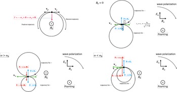

 ω⩾ωB
ω⩾ωB fB=ωB/ω⩾1
 ω=ωB
ω=ωB χp
χp ω<ωB
ω<ωB a0⩽(fB2/3−1)3/2
 a0
a0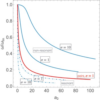
 a0
a0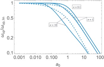
 a0
a0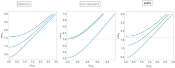
 σ=1
σ=1 a0=0.1, 1, 10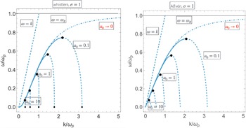
 σ=1
σ=1 k∗−ω∗
k∗−ω∗ ω=0
ω=0 kmax=ωp/a0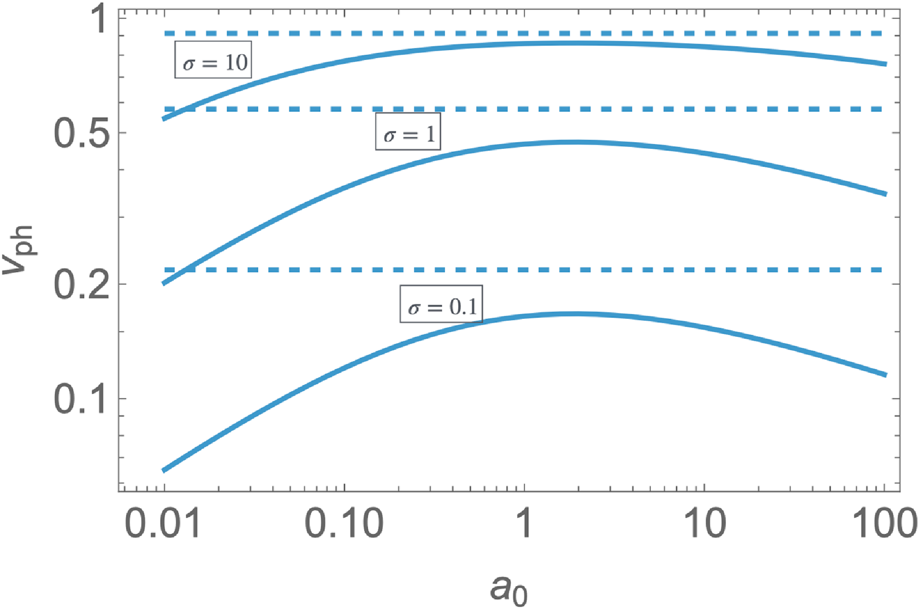
 σ=1
σ=1 k→0
k→0 vA=σ/(2+σ)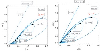
 ηw=Ew/B0
 σ=10
σ=10
 Open access

