


1. Introduction
In layered porous media, the flow of a dense (buoyant) fluid into a buoyant (dense) ambient leads to the formation of gravity currents, where predominantly the flow velocity is aligned with the bottom (top) boundary. Porous media gravity currents are associated with a wide variety of geophysical flows, whether naturally occurring, e.g. seawater contamination of coastal aquifers (Werner et al. Reference Werner, Bakker, Post, Vandenbohede, Lu, Ataie-Ashtiani, Simmons and Barry2013; Costall et al. Reference Costall, Harris, Teo, Schaa, Wagner and Pigois2020), or else related to human activities, e.g. underground hydrogen storage (UHS) (Feldmann et al. Reference Feldmann, Hagemann, Ganzer and Panfilov2016; Tarkowski Reference Tarkowski2019; Muhammed et al. Reference Muhammed, Haq, Al-Shehri, Al-Ahmed, Rahman, Zaman and Iglauer2023) or CO $_2$/acid gas sequestration (Ajayi, Gomes & Bera Reference Ajayi, Gomes and Bera2019; Warnecki et al. Reference Warnecki, Wojnicki, Kusnierczyk and Szuflita2021; Ali et al. Reference Ali, Jha, Pal, Keshavarz, Hoteit and Sarmadivaleh2022). Not surprisingly, a significant volume of research has been driven by the need to understand the dynamics of porous media gravity currents, particularly as they relate to energy industry applications.
In a pioneering study, Huppert & Woods (Reference Huppert and Woods1995) established initial models for porous media gravity current flow. They proposed a similarity solution that was then verified through laboratory experiments. Huppert & Woods (Reference Huppert and Woods1995) showed that a gravity current spreads as  $t^{2/3}$ when fed by a constant-flux source. (Separately, they also derived similarity solutions for a general power-law influx condition.) Many extensions to the Huppert & Woods (Reference Huppert and Woods1995) seminal analysis have been pursued. For example, Hesse et al. (Reference Hesse, Tchelepi, Cantwel and Orr2007), MacMinn et al. (Reference MacMinn, Neufeld, Hesse and Huppert2012), Pegler, Huppert & Neufeld (Reference Pegler, Huppert and Neufeld2014) and Zheng et al. (Reference Zheng, Guo, Christov, Celia and Stone2015) have examined similar examples of buoyancy-driven flow but in porous media that are confined vertically. A question of recent interest, which is more relevant to the research described in this study, is the impact of a heterogeneous porous medium, particularly when some fraction of the injectate is allowed to drain through local or distributed fissures. For example, Anderson, McLaughlin & Miller (Reference Anderson, McLaughlin and Miller2003) investigated the movement of gravity currents in strongly heterogeneous porous media using homogenization methods. They found that by employing appropriate coefficients, one can project the similarity solution appropriate for a (long and thin) gravity current in a uniform medium to gravity current flow in horizontally or vertically layered porous media. Moreover, Pritchard, Woods & Hogg (Reference Pritchard, Woods and Hogg2001) and Farcas & Woods (Reference Farcas and Woods2009) studied distributed drainage over a thin permeable layer. The Pritchard et al. (Reference Pritchard, Woods and Hogg2001) investigation considered miscible flow with drainage along a horizontal layer while Farcas & Woods (Reference Farcas and Woods2009) studied immiscible flow with drainage along an inclined layer. Meanwhile, Neufeld & Huppert (Reference Neufeld and Huppert2009) studied the flow of gravity currents of supercritical $\mathrm {CO_2}$ in thin layers representing the Utsira formation beneath the North Sea. In contrast to the modelling approach of Pritchard et al. (Reference Pritchard, Woods and Hogg2001), who did not consider the possible dynamical influence of the drained fluid on the evolution of the gravity current, Neufeld & Huppert (Reference Neufeld and Huppert2009) hypothesized that when gravity current fluid drains into the interbed layers that separate adjacent permeable layers, such an influence is manifest. More precisely, the weight of the drained fluid adds to the driving force for draining so that, over time, the velocities of drainage and of the gravity current front become respectively large and small. Neufeld & Huppert (Reference Neufeld and Huppert2009) thereby identified three distinct regimes for the drainage of (dense) gravity current fluid, i.e. drainage is driven primarily by (i) the weight of the gravity current, (ii) the combined weight of the gravity current and the fluid already drained into the lower layer, and (iii) the weight of the drained fluid. Regimes (ii) and (iii) are respectively associated with the arrest and retraction of the gravity current front. Similar kinds of flow behaviour have been documented in the related studies of Goda & Sato (Reference Goda and Sato2011), Acton, Huppert & Worster (Reference Acton, Huppert and Worster2001), Sahu & Flynn (Reference Sahu and Flynn2017) and Bharath, Sahu & Flynn (Reference Bharath, Sahu and Flynn2020), who examined, theoretically and experimentally, distributed drainage over a deep lower layer having a relatively small permeability. Most notably, and consistent with Pritchard et al. (Reference Pritchard, Woods and Hogg2001) and Farcas & Woods (Reference Farcas and Woods2009), these related studies found that gravity currents stop elongating when the rate of basal drainage from the gravity current underside matches the source influx.
Most of the above research ignores mass transfer between the gravity current and the ambient fluid saturating the porous medium, e.g. by application of a ‘sharp interface’ assumption in theoretical models. By contrast, and in the context of CO $_2$ sequestration, Neufeld et al. (Reference Neufeld, Hesse, Riaz, Hallworth, Tchelepi and Huppert2010), MacMinn et al. (Reference MacMinn, Neufeld, Hesse and Huppert2012), Pegler et al. (Reference Pegler, Huppert and Neufeld2014) and Khan, Bharath & Flynn (Reference Khan, Bharath and Flynn2022) investigated mixing due to convective dissolution in porous media buoyancy-driven flow. Also, mass transfer processes associated with seawater intrusions into coastal aquifers were considered by Huyakorn et al. (Reference Huyakorn, Andersen, Mercer and White1987) and Paster & Dagan (Reference Paster and Dagan2007). In such examples of miscible porous media flow, the key modes of mass transfer are diffusion and hydrodynamic dispersion. Mixing by dispersion is likewise important when considering the societally important possibility of storing hydrogen (H $_2$) in depleted natural gas reservoirs. Indeed, the combination of H $_2$ leakage through cap-rock and the dispersive mixing of H $_2$ into the ‘cushion gas’ that otherwise occupies the porous medium reduces the volume of H $_2$ that can be recovered economically. Quantifying such details is challenging; e.g. the study by Lubon & Tarkowski (Reference Lubon and Tarkowski2021) estimated the amount of recoverable H $_2$ as anywhere from 50 % to 80 % depending on, among other factors, the number of H $_2$ injection cycles and the degree of heterogeneity within the medium. As regards this latter variable, Feldmann et al. (Reference Feldmann, Hagemann, Ganzer and Panfilov2016) highlighted the possibility of leakage through semi-permeable boundaries by examining H $_2$ migration through a heterogeneous porous medium consisting of sandstone layers separated by tight clay interlayers.
Also in the context of miscibility, Szulczewski & Juanes (Reference Szulczewski and Juanes2013) studied, theoretically, mixing when a fixed amount of dense fluid is released in vertically confined porous media. They reported evidence of various regimes associated with the flow evolution. At early and more especially late times, diffusion is vital, especially when it is coupled with Taylor dispersion. However, at intermediate times, diffusion is insignificant, such that application of the sharp interface assumption is approximately correct. Meanwhile, Sahu & Neufeld (Reference Sahu and Neufeld2020) studied, theoretically and experimentally, the mixing that occurs in a homogeneous porous medium due to velocity-dependant transverse dispersion in gravity currents. In their theoretical model, they exploited mass and buoyancy conservation laws in conjunction with a semi-empirical expression for dispersion, analogue to turbulent entrainment in free shear flows. Sahu & Neufeld (Reference Sahu and Neufeld2020) tuned the associated entrainment coefficient from their theoretical model with measured results from the laboratory. Although transverse dispersion leads, through ‘dispersive entrainment’, to a thickening of the gravity current, the neglect of longitudinal dispersion means that the gravity current length predicted by Sahu & Neufeld (Reference Sahu and Neufeld2020) must match that anticipated by the sharp interface model of Huppert & Woods (Reference Huppert and Woods1995).
The equivalence documented at the end of the previous paragraph runs contrary to the experimental observations of Bharath et al. (Reference Bharath, Sahu and Flynn2020). They studied gravity currents propagating along a permeability jump, and demonstrated that dispersion leads to enhanced gravity current elongation. The difference of length compared to the sharp interface case was attributed to longitudinal dispersion. The Sahu & Neufeld (Reference Sahu and Neufeld2020) model therefore appears most effective in describing gravity current flow through homogeneous media where drainage is not dynamically significant. Recognizing that real geological media are not always so ideal, Sahu & Neufeld (Reference Sahu and Neufeld2023) conducted laboratory experiments to examine dispersive mixing in gravity currents over layered strata. They showed that the mixing that occurs in heterogeneous media is approximately twice that in homogeneous media having otherwise identical properties. To quantify the effects of heterogeneity on mixing, Sahu & Neufeld (Reference Sahu and Neufeld2023) introduced a term called the ‘jump factor’, which characterizes the degree of layering within a porous medium. Sahu & Neufeld (Reference Sahu and Neufeld2023) further demonstrated that the early-time entrainment into the gravity current renders it thick with a rounded nose. Therefore, the long and thin assumption, which is vital in developing a theoretical model, becomes suspect. Sahu & Neufeld (Reference Sahu and Neufeld2023) used their experimental findings to derive semi-empirical equations that estimate the gravity current height and length as functions of time and other parameters. The semi-empirical correlations in question do not, however, distinguish between bulk and dispersed phases within the gravity current. A pioneering theoretical attempt at drawing such a distinction was made by Sahu & Neufeld (Reference Sahu and Neufeld2020), whose approach was later expanded upon by Sheikhi, Sahu & Flynn (Reference Sheikhi, Sahu and Flynn2023). The authors of this latter investigation separated the bulk and dispersed phases to study dispersive mixing in gravity currents elongating over inclined porous media and experiencing local drainage through discrete fissures. Sheikhi et al. (Reference Sheikhi, Sahu and Flynn2023) thereby extended the theoretical model of Sahu & Neufeld (Reference Sahu and Neufeld2020) by introducing two entrainment velocities, i.e.  $w_{e1}$, which is associated with entrainment from the bulk phase to the dispersed phase, and $w_{e2}$, which is associated with entrainment from the surrounding ambient to the dispersed phase. They assumed an identical entrainment coefficient associated with $w_{e1}$ and $w_{e2}$, and determined the numerical value of this entrainment coefficient by fitting theoretical predictions against COMSOL-based numerical simulations meant to mimic similitude laboratory experimental conditions. Their theoretical model, combined with the COMSOL numerical simulations, revealed that five parameters can affect the amount of dispersive mixing in porous media gravity currents experiencing local drainage: (i) $\varGamma$, which represents flow conditions upstream of the local fissure(s); (ii) $K$, which represents the permeability ratio (fissure-to-medium); (iii) $\xi$, which represents the fissure width; (iv) $l$, which represents the fissure depth; and (v) $\theta$, which represents the dip angle.
A primary objective of this study is to extend the work of Sheikhi et al. (Reference Sheikhi, Sahu and Flynn2023) to gravity currents experiencing distributed drainage, as is more representative of many geological flows compared to the case of localized drainage. To do so, we suppose that the gravity current propagates through a porous medium and over a thin interbed layer having a lower – possibly substantially lower – permeability. We develop a theoretical model and a complementary numerical model to study the details of the dispersive mixing relevant to this case. In the former case, our formulation is predicated on two linearizations of the real behaviour. The first pertains to fluid mechanics and supposes a linear entrainment law of the type proposed for high-Reynolds-number shear flows by Ellison & Turner (Reference Ellison and Turner1959) and for low-Reynolds-number porous media flows by Sahu & Neufeld (Reference Sahu and Neufeld2020). The second pertains to thermodynamics and supposes a linear equation of state, i.e. a linear relationship between fluid density and solute concentration. The latter linearization in particular seems well-justified in a UHS context: measured data from Hassanpouryouzband et al. (Reference Hassanpouryouzband, Joonaki, Edlmann, Heinemann and Yang2020) suggest that nonlinear terms in the equation of state describing H $_2$/CH $_4$ mixtures have minor significance. Meanwhile, the validity of the former linearization is discussed in more detail below. A further objective of our study is to characterize the drainage of gravity current fluid into the interbed layer and, from there, into a semi-infinite layer of larger permeability below. (For analytical convenience and consistent with previous studies – e.g. Huppert & Woods (Reference Huppert and Woods1995), Neufeld & Huppert (Reference Neufeld and Huppert2009), Bharath et al. (Reference Bharath, Sahu and Flynn2020) and Sahu & Neufeld (Reference Sahu and Neufeld2023) – we assume a dense rather than a light gravity current. As a result, the gravity current appears ‘upside down’ relative to those expected e.g. in UHS-type flows. Note, however, that the flow orientation does not impact the flow dynamics provided that we apply the Boussinesq approximation, which supposes relatively modest density differences between the injectate and the ambient fluid.)
The rest of the paper is organized as follows. Section 2 derives the theoretical model for the gravity current by incorporating a distributed drainage formulation. Particular attention is paid to two limiting cases, which assume either no mixing or perfect mixing in the lowest of the porous layers. In § 3, we outline the COMSOL-based numerical simulations conducted to validate and contextualize the predictions of the theoretical model. In § 4, we discuss these predictions in more detail, and contrast the predictions with complementary output from the numerical simulations. Finally, key findings of the current work are reviewed, and prospects for future research are identified, in § 5.
2. Theoretical model
2.1. Governing equations
We examine the flow of a gravity current,  $z\geq 0$ in figure 1, that occurs when a dense fluid with density $\rho _s$ is injected into a uniform porous medium with constant permeability $k$. This medium is intersected by a thin interbed layer of permeability $k_b< k$ with inclination angle $\theta$ and depth $\xi$. Thus the interbed layer occupies the vertical expanse $-\xi < z < 0$. In general, and with the application of (buoyant) H $_2$ storage in an anticline structure in mind, we consider an up-dip inclination angle. The $(x,z)$ coordinate system that describes the directions along and perpendicular to the slope is derived by rotating the natural coordinates $(X,Z)$ in a clockwise direction by the dip angle $\theta$. The red dot shown in figure 1 signifies the isolated source, and the origin for both coordinate systems is located at this same point.

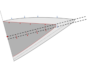
Figure 1. Schematic of a leaky gravity current propagating along, and draining through, the permeability jump associated with an interbed layer of thickness  $\xi$. We assume equal permeability $k$ in the upper and lower layers, and a reduced permeability $k_b$ in the interbed layer. The gravity current and the fluid that drains from the gravity current consist of bulk and dispersed phases. These are, respectively, confined by the red and black curves. Meanwhile, the dashed curve that is drawn through the lower two layers signifies the equivalent depth of draining fluid, assuming that this draining fluid consists solely of bulk fluid, i.e. has a density that matches the source density. The variables $h_1$, $h_2$, $u_1$, $u_2$, $w_{e1}$, $w_{e2}$ and $\bar {c}_2$ depend on $x$ and $\tilde {t}$. Conversely, the variables $x_{N_b}$ and $x_{N_d}$ depend only on $\tilde {t}$. The vertical scale is exaggerated in this schematic.
The continuity equation for the bulk (or unmixed) phase of the gravity current experiencing drainage over its lower boundary reads
 \begin{equation} \frac{\partial h_1}{\partial \tilde{t}} + \frac{\partial }{\partial x}(u_1 h_1) ={-} w_{e1} -w_{d1}. \end{equation}
Here,  $h_1$ is the height of the bulk phase, $u_1$ is the bulk phase velocity, and $w_{e1}$ and $w_{d1}$ are velocities that respectively account for entrainment from the bulk to the dispersed phase and drainage from the bulk phase through the lower layer. Also, $\tilde {t}= t/ \phi$, in which $\phi$ is the porosity. (Note that all velocities in our theoretical model are Darcy velocities.)
Similarly, the continuity equation for the dispersed phase can be stated as
 \begin{equation} \frac{\partial h_2 }{\partial \tilde{t}} + \frac{\partial }{\partial x} [u_2(h_2-h_1)] ={-}\frac{\partial }{\partial x}(u_1 h_1) + w_{e2}-w_{d1}-w_{d2}, \end{equation}
where  $h_2-h_1$ is the thickness of the dispersed phase, $u_2$ (assumed independent of $z$) is the advection speed of the dispersed phase, $w_{e2}$ is the entrainment velocity from the ambient to the dispersed phase, and $w_{d2}$ is the drainage velocity from the dispersed phase through the lower layer. The latter velocity must be interpreted with some care because it is not defined everywhere along the extent $0 \leq x \leq x_{N_d}$ occupied by the dispersed phase (and likewise for $w_{d1}$). We clarify this situation when formally defining the draining velocities $w_{d1}$ and $w_{d2}$ below.
Although the solute concentration in the bulk phase is equal to the source concentration  $c_s$ by assumption, the concentration in the dispersed phase varies between $0$ and $c_s$. Therefore a $z$-averaged solute concentration $\bar {c}_2$ is defined in the dispersed phase. Solute conservation in the dispersed phase can be expressed as
 \begin{equation} \frac{\partial b_2}{\partial \tilde{t}} + \frac{\partial }{\partial x}(u_2 b_2) = w_{e1}c_s\,\mbox{H}(x_{N_b}-x)-w_{d2}\bar{c}_2, \end{equation}
in which  $b_2=\bar {c}_2(h_2-h_1)$ is the buoyancy of the dispersed phase, averaged over depth. Meanwhile $\mbox {H}(x_{N_b}-x)$ is a Heaviside step function, which is zero everywhere except when $x_{N_b} > x$, where $x_{N_b}$ indicates the front position of the bulk phase. In this study, we follow previous work on entraining flows from either the turbulent free shear flow literature (e.g. Ellison & Turner Reference Ellison and Turner1959) or, much more importantly, the porous media flow literature (e.g. Sahu & Neufeld Reference Sahu and Neufeld2020), and so consider a linear entrainment relationship. Accordingly, the entrainment velocities are defined as $w_{e1}=\varepsilon u_1$ and $w_{e2}=\varepsilon u_2$, where $\varepsilon$ is the dispersive entrainment coefficient. Extrapolation of these relationships to more complicated formulations (e.g. $w_{e1}=\varepsilon _1 u_1$ and $w_{e2}=\varepsilon _2 u_2$ with $\varepsilon _1 \neq \varepsilon _2$, or $w_{ei} \propto u_i^\lambda$ or $w_{e1} \propto |u_1-u_2|$) remains a topic to be examined in future studies. Our reluctance to pursue such a line of inquiry here stems not from the physical illogicality of these alternative formulations but rather from our desire to minimize model complexity and the number of variables whose value must be set by comparison with numerical output.
By considering a hydrostatic pressure gradient throughout the gravity current and using Darcy's law, the horizontal velocity in each phase is given by
 $$\begin{gather} u_1(x,\tilde{t})={-}\frac{kg\beta}{\nu} \left[\frac{\partial b_2}{\partial x}\cos\theta +c_s\left(\frac{\partial h_1}{\partial x}\cos\theta+\sin\theta\right)\right], \end{gather}$$
 $$\begin{gather}u_2(x,\tilde{t})={-}\frac{kg\beta}{\nu}\left[\frac{\partial (\bar{c}_2 h_2)}{\partial x}\cos\theta+\bar{c}_2\sin\theta\right] \equiv{-}\frac{kg\beta}{\nu}\left[\frac{\partial }{\partial x} \left(\frac{b_2h_2}{h_2-h_1} \right)\cos\theta+\bar{c}_2\sin\theta\right] \end{gather}$$
(see Sheikhi et al. Reference Sheikhi, Sahu and Flynn2023). Here,  $\beta$ is the solute contraction coefficient, which we borrow from the (assumed linear) equation of state $\rho =\rho _0(1+\beta c)$ in which $\rho _0$ is the density of the uncontaminated ambient fluid. Also, $\nu$ is the kinematic viscosity, which we assume to be the same throughout the bulk and dispersed phases. By inserting (2.4)–(2.5) and the expressions for the entrainment velocities $w_{e,1}$ and $w_{e,2}$ into (2.1)–(2.3), we obtain the following modified governing equations:
 \begin{gather} \frac{\partial h_1}{\partial \tilde{t}} +\frac{k g^{\prime}_s }{\nu}\,\frac{\partial (h_1U)}{\partial x} ={-}\varepsilon\,\frac{k g^{\prime}_s }{\nu}\,U -w_{d1}, \end{gather}
 \begin{gather} \frac{\partial h_2}{\partial \tilde{t}} -\frac{k g^{\prime}_s }{\nu}\,\frac{\partial }{\partial x} \left[(h_2-h_1)\left(\frac{\partial \varPsi }{\partial x}+C\sin\theta \right) -h_1 U\right] \nonumber\\ ={-}\varepsilon\,\frac{k g^{\prime}_s }{\nu}\left(\frac{\partial \varPsi }{\partial x}+C\sin\theta\right) -w_{d1}-w_{d2}, \end{gather}
 \begin{gather} \frac{\partial b_2}{\partial \tilde{t}} -\frac{k g^{\prime}_s }{\nu}\,\frac{\partial }{\partial x} \left[b_2 \left(\frac{\partial \varPsi}{\partial x}+C\sin\theta\right)\right] = \varepsilon\,\frac{k g^{\prime}_s }{\nu}\,Uc_s\,\mbox{H}(x_{N_b}-x) -w_{d2}Cc_s. \end{gather}
In the above equations, we have introduced the following symbols:
 $$\begin{gather} U={-}\left(\frac{1}{c_s}\,\frac{\partial b_2}{\partial x} + \frac{\partial h_1}{\partial x}\right)\cos\theta- \sin\theta, \end{gather}$$
 $$\begin{gather}\varPsi=\frac {b_2 h_2}{c_s(h_2-h_1)}\cos\theta, \end{gather}$$
 $$\begin{gather}C=\frac {\bar{c}_2 }{c_s} \equiv \frac {b_2 }{c_s(h_2-h_1)}. \end{gather}$$
Note that  $U$,
$U$,  $\varPsi$ and $C$ are defined solely for the purpose of simplifying our notation, i.e these variables do not carry any particular physical meaning. Before studying (2.6)–(2.8) in more detail, it is necessary to define the drainage velocities $w_{d1}$ and $w_{d2}$. These velocities are influenced by the degree of mixing occurring in the lower layer of the porous medium. Because predicting the extent of mixing in this lower layer is a complicated task that relies on numerous factors (see e.g. figure 10 in Bharath et al. (Reference Bharath, Sahu and Flynn2020), and the discussion thereof), we will confine ourselves to two limiting scenarios, which we label as perfect mixing and no mixing. Both of the perfect mixing and no mixing cases are idealizations. Consistent with Pritchard et al. (Reference Pritchard, Woods and Hogg2001), the former assumes that dense fluid that drains through the interbed layer immediately dissolves into lower layer ambient fluid. Meanwhile the latter scenario supposes that mixing details can be ignored in this lower layer (even though they figure prominently in our description of the gravity current flow). Thus we assume that the draining flows evolve as depicted in figure 1. The perfect mixing and no mixing idealizations are helpful bookend-limiting cases that we expect to often bound the true behaviour of the evolving flow.
2.1.1. Perfect mixing
As noted above, the perfect mixing regime considers an immediate and total dissolution of drained gravity current fluid when this dense fluid reaches the lower layer. In turn, and because this lower layer is semi-infinite in extent, it maintains a negligible solute concentration. The perfect mixing regime is supposed to be approached when the density difference between the gravity current fluid and the ambient fluid is comparatively large, or when the permeability in the interbed layer is much smaller than elsewhere. As suggested by figure 2, perfect mixing is analogous to a situation where drained fluid is removed from the domain as soon as it exits the interbed layer. Note that such a removal does not invalidate equations (2.6)–(2.11), which are focused on the flow dynamics in the domain  $z > 0$.

Figure 2. Schematic of a leaky gravity current experiencing perfect mixing in (and therefore immediate removal from) the lower layer. The red line indicates the bulk interface, and the black curve indicates the dispersed interface.
From figure 2, the drainage velocities  $w_{d1}$ and $w_{d2}$ can be determined by using the $z$-component of Darcy's law, i.e.
 \begin{equation} \frac{\partial p}{\partial z}={-} \rho g^{\prime}\cos\theta-\frac{\mu}{k}\,w, \end{equation}
where  $\mu$ is the dynamic viscosity, $p$ is the pressure, and $g^{\prime }=g\beta c$ is the reduced gravity. We enforce continuity of pressure and of the vertical flux at $z=0$, and thereby conclude that
 \begin{equation}
w_{d1}(x,\tilde{t})=\left\{\begin{array}{@{}ll} \dfrac{k_b
g^{\prime}_s }{\nu} \left(\dfrac{c_sh_1+b_2}{c_s
\xi}+1\right)\cos\theta, & 0 \leq x <
x_{N_b}, \\ 0, & x_{N_b} \leq x \leq
x_{N_d}. \end{array}\right.
\end{equation}
\begin{equation}
w_{d1}(x,\tilde{t})=\left\{\begin{array}{@{}ll} \dfrac{k_b
g^{\prime}_s }{\nu} \left(\dfrac{c_sh_1+b_2}{c_s
\xi}+1\right)\cos\theta, & 0 \leq x <
x_{N_b}, \\ 0, & x_{N_b} \leq x \leq
x_{N_d}. \end{array}\right.
\end{equation}
This last result considers the draining of bulk phase fluid through the upper and interbed layers. Meanwhile, and by examining the dispersed phase, it can be shown that
 \begin{equation}
w_{d2}(x,\tilde{t})=\left\{\begin{array}{@{}ll} 0, &
0 \leq x < x_{N_b}, \\ \dfrac{k_b g^{\prime}_s
}{\nu}\,C \left(\dfrac{h_2}{\xi}+1\right)\cos
\theta, & x_{N_b} \leq x \leq x_{N_d}.
\end{array}\right.
\end{equation}
\begin{equation}
w_{d2}(x,\tilde{t})=\left\{\begin{array}{@{}ll} 0, &
0 \leq x < x_{N_b}, \\ \dfrac{k_b g^{\prime}_s
}{\nu}\,C \left(\dfrac{h_2}{\xi}+1\right)\cos
\theta, & x_{N_b} \leq x \leq x_{N_d}.
\end{array}\right.
\end{equation}
(The derivation of (2.13) and (2.14) is outlined in Appendix A.) Note that the (degenerate) limit  $\xi \to 0$ is not necessarily associated with the appearance of singularities in (2.13) and (2.14) because $\xi \to 0$ likewise implies $k_b \to 0$.
2.1.2. No mixing
If no mixing occurs in the lower layer, then the solute concentration of the drained fluid is the same as the solute concentration of the gravity current fluid directly above it. In this case, the drainage velocities are obtained by applying (2.12) for both the bulk and dispersed phases and through all three layers of figure 1. That is,
 \begin{equation}
w_{d1}(x,\tilde{t})=\left\{\begin{array}{@{}ll} \dfrac{k_b
g^{\prime}_s }{\nu}\cos \theta \left\{\begin{array}{@{}ll}
\left(\dfrac{c_sh_1+b_2}{c_sl}+1\right), & l < \xi, \\ \dfrac{c_sh_1+b_2+c_s l}{(1-K)c_s\xi+Kc_s
l}, & l \geq \xi, \end{array}\right. & 0
\leq x < x_{N_b}, \\ 0, & x_{N_b} \leq x
\leq x_{N_d}, \end{array}\right.
\end{equation}
\begin{equation}
w_{d1}(x,\tilde{t})=\left\{\begin{array}{@{}ll} \dfrac{k_b
g^{\prime}_s }{\nu}\cos \theta \left\{\begin{array}{@{}ll}
\left(\dfrac{c_sh_1+b_2}{c_sl}+1\right), & l < \xi, \\ \dfrac{c_sh_1+b_2+c_s l}{(1-K)c_s\xi+Kc_s
l}, & l \geq \xi, \end{array}\right. & 0
\leq x < x_{N_b}, \\ 0, & x_{N_b} \leq x
\leq x_{N_d}, \end{array}\right.
\end{equation}
and
 \begin{equation}
w_{d2}(x,\tilde{t})=\left\{\begin{array}{@{}ll} 0, &
0 \leq x < x_{N_b}, \\ \dfrac{k_b g^{\prime}_s
}{\nu}\cos \theta \left\{\begin{array}{@{}ll}
\left(\dfrac{h_2}{l}+1\right), & l < \xi,
\\ \dfrac{h_2+l}{(1-K)\xi+Kl}, & l \geq
\xi, \end{array}\right. & x_{N_b} \leq x \leq
x_{N_d}. \end{array}\right.
\end{equation}
\begin{equation}
w_{d2}(x,\tilde{t})=\left\{\begin{array}{@{}ll} 0, &
0 \leq x < x_{N_b}, \\ \dfrac{k_b g^{\prime}_s
}{\nu}\cos \theta \left\{\begin{array}{@{}ll}
\left(\dfrac{h_2}{l}+1\right), & l < \xi,
\\ \dfrac{h_2+l}{(1-K)\xi+Kl}, & l \geq
\xi, \end{array}\right. & x_{N_b} \leq x \leq
x_{N_d}. \end{array}\right.
\end{equation}
(The derivation of (2.15) and (2.16) is outlined in Appendix B.) No corresponding expressions are provided for  $u_{d1}$ and $u_{d2}$ because in the rotated or $(x,z)$ coordinate system, $u_{d1}$ and $u_{d2}$ do not impact the evolution of $l$.) Here, $K={k_b}/{k}$ is the permeability ratio. When $\xi \to \infty$, (2.15)–(2.16) are consistent with the drainage formulation of Acton et al. (Reference Acton, Huppert and Worster2001) for a gravity current propagating over a deep layer that is permeable but ‘tight’. By contrast, we again avoid consideration of the limit $\xi \to 0$: in the absence of an interbed layer, figure 1 must be redrawn completely because source fluid will now fall vertically in the form of a descending plume. Such a flow, studied at some length by Sahu & Flynn (Reference Sahu and Flynn2015) and Gilmore et al. (Reference Gilmore, Sahu, Benham, Neufeld and Bickle2021), is not the focus of the current work.
Finally, and in defining the depth of the contaminated fluid in the lower layer, we simplify the analysis by defining  $l(x,\tilde {t})$ as an equivalent depth such that all of the drained fluid in the lower layer has the same uniform solute concentration $c_s$. The evolution equation for $l$ therefore reads
 \begin{equation} \frac{\partial l}{\partial \tilde{t}}=\left\{\begin{array}{@{}ll} w_{d1}, & 0 \leq x < x_{N_b}, \\[2pt] Cw_{d2}, & x_{N_b} \leq x \leq x_{N_d}. \end{array}\right.\end{equation}
In solving (2.17), we acknowledge that we do not distinguish rigorously between the bulk and dispersed phases for  $z < 0$. On the other hand, no such sacrifice applies for $z>0$, thus our dynamical description of the bulk and dispersed phases of the gravity current is not jeopardized.
2.2. Boundary conditions
As shown in Sheikhi et al. (Reference Sheikhi, Sahu and Flynn2023), boundary conditions for a gravity current consisting of bulk and dispersed phases are
 $$\begin{gather} -\frac{kg^{\prime}_s}{\nu}\left[\left(\frac{1}{c_s}\,\frac{\partial b_2}{\partial x} + \frac{\partial h_1}{\partial x}\right)h_1\cos\theta +h_1 \sin\theta\right]_{0}=q_s,\quad h_1\vert_{x_{N_b}} =0, \end{gather}$$
 $$\begin{gather}h_2\vert_{0} =h_1\vert_{0},\quad h_2\vert_{x_{N_d}} =0, \end{gather}$$
 $$\begin{gather}b_2\vert_{0} =0,\quad b_2\vert_{x_{N_d}} =0. \end{gather}$$
Whereas the last five of these expressions are self-explanatory, the first (influx) boundary condition merits some additional discussion. In this spirit, (2.18a) signifies that all of the injectate supplied by the source is added to the rear of the gravity current such that the source volume flux matches the gravity current volume flux measured at  $x=0$. Thereafter, and consistent with the numerical treatment of the source to be described in § 3, gravity current fluid may propagate down-dip or else drain into the interbed layer.
2.3. Non-dimensional governing equations
Following Goda & Sato (Reference Goda and Sato2011), we define a characteristic length scale  $\varPi _1$ and a characteristic time scale $\varPi _2$ as
 \begin{equation} \varPi_1=\frac{\nu q_s}{k g^\prime_s}\quad \mbox{and}\quad \varPi_2 = q_s\left(\frac{\nu}{kg^\prime_s}\right)^2, \end{equation}
respectively. Thus we define the following dimensionless (starred) variables:
 \begin{equation} \left.\begin{gathered} x^* = \frac{x}{\varPi_1},\quad \xi^* = \frac{\xi}{\varPi_1},\quad h_1^* = \frac{h_1}{\varPi_1},\quad h_2^* = \frac{h_2}{\varPi_1},\\ l^* = \frac{l}{\varPi_1},\quad t^* = \frac{\tilde{t}}{\varPi_2},\quad w^* = w\frac{\varPi_2}{\varPi_1}. \end{gathered}\right\} \end{equation}
Also,  $c_2^*={c_2}/{c_s}$. Note that for notational simplicity, we drop the superscript $^*$ such that all variables are now to be interpreted as dimensionless. (By necessity, however, we revert to dimensional variables in § 3.1 and in the appendices.) Accordingly, (2.6)–(2.8) may be rewritten as
 $$\begin{gather} \frac{\partial h_1}{\partial t} +\frac{\partial (h_1U)}{\partial x} ={-}\varepsilon U -w_{d1}, \end{gather}$$
 $$\begin{gather}\frac{\partial h_2}{\partial t} -\frac{\partial }{\partial x} \left[(h_2-h_1)\left(\frac{\partial \varPsi}{\partial x}+C\sin\theta \right) -h_1 U\right] ={-} \varepsilon \left(\frac{\partial \varPsi}{\partial x}+C\sin\theta\right) -w_{d1}-w_{d2}, \end{gather}$$
 $$\begin{gather}\frac{\partial b_2}{\partial t} -\frac{\partial }{\partial x} \left[b_2 \left(\frac{\partial \varPsi}{\partial x}+C\sin \theta\right)\right] = \varepsilon U\,{\rm H}(x_{N_b}-x) -w_{d2}C. \end{gather}$$
Here,
 $$\begin{gather} b_2=c_2(h_2-h_1), \end{gather}$$
 $$\begin{gather}U={-}\left(\frac{\partial b_2}{\partial x} +\frac{\partial h_1}{\partial x}\right)\cos\theta- \sin\theta, \end{gather}$$
 $$\begin{gather}\varPsi=\frac{b_2 h_2}{h_2-h_1}\cos\theta, \end{gather}$$
 $$\begin{gather}C= \frac{b_2}{h_2-h_1}. \end{gather}$$
Equations (2.21)–(2.23) comprise three equations in three unknowns, namely  $h_1$, $h_2$ and $b_2$. The dimensionless boundary conditions to be coupled to these equations read
 $$\begin{gather} \left[\left(\frac{\partial b_2}{\partial x} +\frac{\partial h_1}{\partial x}\right)h_1\cos\theta + h_1 \sin\theta\right]_{0}={-}1,\quad h_1\vert_{x_{N_b}} =0, \end{gather}$$
 $$\begin{gather}h_2\vert_{0} =h_1\vert_{0},\quad h_2\vert_{x_{N_d}} =0, \end{gather}$$
 $$\begin{gather}b_2\vert_{0} =0,\quad b_2\vert_{x_{N_d}} =0. \end{gather}$$
When a state of perfect mixing can be assumed for the lower layer, the dimensionless drainage velocities that appear in (2.21)–(2.23) are given by
 \begin{equation} w_{d1}=K\cos \theta\left\{\begin{array}{@{}ll} \left(\dfrac{h_1+b_2}{\xi}+1\right), & 0 \leq x < x_{N_b}, \\ 0, & x_{N_b} \leq x \leq x_{N_d}, \end{array}\right. \end{equation}
and
 \begin{equation} w_{d2}=K\cos \theta\left\{\begin{array}{@{}ll} 0, & 0 \leq x < x_{N_b}, \\ C\left(\dfrac{h_2}{\xi}+1\right), & x_{N_b} \leq x \leq x_{N_d}, \end{array}\right. \end{equation}
where  $K$ is the aforementioned permeability ratio. For the no mixing case, by contrast, we write
 \begin{equation}
w_{d1}=\left\{\begin{array}{@{}ll} K\cos \theta
\left\{\begin{array}{@{}ll}
\left(\dfrac{h_1+b_2}{l}+1\right), & l <
\xi, \\ \dfrac{h_1+b_2+l}{(1-K)\xi+Kl}, &
l \geq \xi, \end{array}\right. & 0 \leq x <
x_{N_b}, \\ 0, & x_{N_b} \leq x \leq
x_{N_d}, \end{array}\right. \end{equation}
\begin{equation}
w_{d1}=\left\{\begin{array}{@{}ll} K\cos \theta
\left\{\begin{array}{@{}ll}
\left(\dfrac{h_1+b_2}{l}+1\right), & l <
\xi, \\ \dfrac{h_1+b_2+l}{(1-K)\xi+Kl}, &
l \geq \xi, \end{array}\right. & 0 \leq x <
x_{N_b}, \\ 0, & x_{N_b} \leq x \leq
x_{N_d}, \end{array}\right. \end{equation}
and
 \begin{equation}
w_{d2}=\left\{\begin{array}{@{}ll} 0, & 0 \leq x <
x_{N_b}, \\ K\cos \theta \left\{\begin{array}{@{}ll}
\left(\dfrac{h_2}{l}+1\right), & l < \xi,\\
\dfrac{h_2+l}{(1-K)\xi+Kl}, & l \geq \xi, \end{array}\right. & x_{N_b} \leq x \leq
x_{N_d}. \end{array}\right.
\end{equation}
\begin{equation}
w_{d2}=\left\{\begin{array}{@{}ll} 0, & 0 \leq x <
x_{N_b}, \\ K\cos \theta \left\{\begin{array}{@{}ll}
\left(\dfrac{h_2}{l}+1\right), & l < \xi,\\
\dfrac{h_2+l}{(1-K)\xi+Kl}, & l \geq \xi, \end{array}\right. & x_{N_b} \leq x \leq
x_{N_d}. \end{array}\right.
\end{equation}
Finally, the non-dimensional analogue of (2.17) becomes
 \begin{equation} \frac{\partial l}{\partial t}=\left\{\begin{array}{@{}ll} w_{d1}, & 0 \leq x < x_{N_b}, \\[2pt] Cw_{d2}, & x_{N_b} \leq x \leq x_{N_d}. \end{array}\right. \end{equation}
 An explicit finite difference algorithm is employed to solve the governing equations. This approach discretizes spatial derivatives using backward finite differences. Note that, so as to prevent unrealistic singularities, we initialize  $l$ with a small value, i.e. $l(x,0) = 10^{-3}$. Figures 3(a,b) show results for both the perfect mixing and no mixing cases. Because $l$ is comparable to $\xi$ at early times, the prediction for $w_{d1}$ returned by (2.29) is similar to that returned by (2.31), and likewise when considering $w_{d2}$, for (2.30) and (2.32). As a result, and up to $t \simeq 100$, the gravity current propagates to a comparable extent in both scenarios. As time evolves, the $l$ predicted by (2.33) for the no mixing case increases steadily. When $l$ is similar in magnitude to $h_2$, the drainage velocity remains small such that the gravity current extends beyond the steady-state value that is realized in the long-time limit. As $l$ continues to increase, however, the gravity current begins to retract, a pattern clearly evident from figure 3(b). This pattern of extension and retraction is quite different from that noted in the perfect mixing case, where the terminal length of the gravity current is approached monotonically. The difference in behaviour in question therefore provides a convenient metric by which to assess the validity of one versus the other representation of lower layer mixing. However, before elaborating on such details and the results anticipated away from the bookend-limiting cases of figures 3(a,b), it is first necessary to summarize the numerical technique used to resolve such flows.

Figure 3. Theoretical predictions showing gravity current profiles assuming (a) perfect mixing, and (b) no mixing in the lower layer. Thick lines represent the bulk interface, and thin lines represent the dispersed interface. Here,  $K=0.0025$, $\xi =0.333$ (equivalent to $K_{{eff}} \equiv K(1+{1}/{\xi }) = 0.01$) and $\theta =0^\circ$. We further assume that $\varepsilon =0.0344$. The justification for this choice will be presented in § 3.4.
3. Numerical simulations
The first purpose of the COMSOL-based numerical simulations is to approximate the value of  $\varepsilon$ in the theoretical models of § 2. Thereafter, we use numerical results to infer the strengths and weaknesses of the perfect mixing and no mixing models.
Consistent with the orientation of the flows depicted in figures 1 and 2, we consider the evolution of a dense gravity current through a less dense ambient. More precisely, and mimicking similitude laboratory experiments, we assume that the gravity current and ambient fluids are respectively comprised of salt and fresh water. Although this choice guides our selection of the equation of state, the results of § 4 are, in any event, non-dimensionalized so as to add a degree of generality to our numerically computed calculations. Notwithstanding this preference for non-dimensional variables, it must be noted that  $g^\prime _s=15$ and $q_s=0.3$ cm $^2$ s $^{-1}$ in our simulations. Typically, simulations are run for 20 minutes after injection onset, representing an investment of approximately 30 hours of wall-clock time on an Intel Core i7-9700 CPU with 3.00 GHz and 16 GB memory. (By comparison, solving numerically the theoretical model of § 2 requires only about 3 % of the computational resources needed for the COMSOL simulations.)
3.1. COMSOL set-up
In order to determine the velocity and concentration fields in our numerical simulations, mass continuity, Darcy's equation and a solute transport equation are solved. With COMSOL, this is achieved by leveraging the following two interfaces.
(i) The Darcy's law (dl) interface prescribes the mass and momentum equations as
(3.1a) $$\begin{gather} \frac{\partial u}{\partial x}+\frac{\partial w}{\partial z}=0, \end{gather}$$(3.1b)$$\begin{gather}\frac{1}{\rho_0}\,\frac{\partial p}{\partial x}+\frac{\nu}{k}\,u=\frac{\rho}{\rho_0}\,g\sin\theta, \end{gather}$$(3.1c)respectively.$$\begin{gather}\frac{1}{\rho_0}\,\frac{\partial p}{\partial z}+\frac{\nu}{k}\,w=\frac{\rho}{\rho_0}\,g\cos\theta, \end{gather}$$
(ii) The transport of diluted species in porous media (tds) interface solves the solute transport equation
(3.2)\begin{align} \phi\,\frac{\partial c}{\partial t}+ u\,\frac{\partial c}{\partial x}+w\, \frac{\partial c}{\partial z}=\phi\left[\frac{\partial}{\partial x} \left({\mathsf{D}}_{xx}\,\frac{\partial c}{\partial x}+{\mathsf{D}}_{xz}\,\frac{\partial c}{\partial z}\right)+ \frac{\partial}{\partial z} \left({\mathsf{D}}_{xz}\,\frac{\partial c}{\partial x}+{\mathsf{D}}_{zz}\, \frac{\partial c}{\partial z}\right)\right]. \end{align}


Here,  $c$ is the solute concentration, and ${\mathsf{D}}_{xx}$, ${\mathsf{D}}_{xz}$ and ${\mathsf{D}}_{zz}$ are components of the dispersion tensor, ${\mathsf{D}}_{ij}$. As explained by Bear (Reference Bear1972), this tensor can be defined based on two independent variables, namely the longitudinal dispersivity $a_L$ and the transverse dispersivity $a_T$, i.e.
 $$\begin{gather} {\mathsf{D}}_{xx}={\mathsf{D}}_{mol}+a_L\,\frac{u^2}{|\boldsymbol{V}|}+a_T\,\frac{w^2}{|\boldsymbol{V}|}, \end{gather}$$
 $$\begin{gather}{\mathsf{D}}_{zz}={\mathsf{D}}_{mol}+a_L\,\frac{w^2}{|\boldsymbol{V}|}+a_T\frac{u^2}{|\boldsymbol{V}|}, \end{gather}$$
 $$\begin{gather}{\mathsf{D}}_{xz}={\mathsf{D}}_{mol}+(a_L-a_T)\,\frac{|uw|}{|\boldsymbol{V}|}, \end{gather}$$
where  ${\mathsf{D}}_{mol}$ is the coefficient of molecular diffusion, and $|\boldsymbol {V}|$ is overall velocity magnitude. Following Sheikhi et al. (Reference Sheikhi, Sahu and Flynn2023), the dispersivity parameters $a_L$ and $a_T$ are predicted based on the empirical correlations of Delgado (Reference Delgado2007) as
 \begin{equation} a_L=\left\{\begin{array}{@{}ll} 0.5d_p, & 300<{Pe}<10^5, \\[2pt] 0.025d_p, & 300<{Pe}<10^5, \end{array}\right.\quad a_T = 0.025d_p, \end{equation}
in which  ${Pe}$ is the Péclet number, and $d_p$ is the bead diameter. In this work, we consider $d_p = 0.5$ mm in line with similitude experiments of the type performed by Sahu & Flynn (Reference Sahu and Flynn2017) and Bharath et al. (Reference Bharath, Sahu and Flynn2020). Note finally that the linear equation of state $\rho =\rho _0 (1+\beta c)$ allows us to relate the density in (3.1b,c) with the solute concentration in (3.2).
3.2. Initial conditions and solver
Initially, it is assumed that the porous medium is filled with fresh water of density  $\rho _0=0.998$ g cm $^{-3}$ such that the solute concentration is zero at $t=0$. The source consists of an opening, oriented in $z$, of height 5 mm across which salt water is injected in $x$ with a uniform velocity profile. We determine the salt water density from $g^\prime _s$ by applying
 \begin{equation} \rho_s=\left(1+\frac{g^\prime_s}{g}\right)\rho_0. \end{equation}
To discretize (3.1) and (3.2), an unstructured triangular mesh (with local refinement in the neighbourhood of the source) is employed – see figure 4. After performing a grid independency study, the governing equations are discretized in space using cubic shape functions for (3.1) and quadratic shape functions for (3.2). A third-order implicit backward differentiation formula is employed for time discretization.

Figure 4. Schematic of the numerical set-up for similitude (a) perfect mixing and (b) laboratory experiments.
3.3. Preliminary validation
As described in more detail in Sheikhi et al. (Reference Sheikhi, Sahu and Flynn2023), our COMSOL model is validated using different points of reference. First, we model the flow of a porous media gravity current along an impermeable boundary and observe strong agreement with the theoretical solution of Huppert & Woods (Reference Huppert and Woods1995). This comparison confirms the effectiveness of the COMSOL model in predicting porous media buoyancy-driven flow (without either drainage or dispersion). Second, we confirm that our COMSOL model predicts accurately the amount of dispersion experienced by a passive scalar by juxtaposing numerical model output with the classical solution of Bear (Reference Bear1972), § 10.6. This comparison confirms the effectiveness of the COMSOL model in predicting dispersion (without buoyancy effects). Finally, we compare numerical predictions against the flow patterns observed in similitude laboratory experiments of a filling box flow consisting of a leaky gravity current fed by a descending plume, i.e. figures 4(a,c) of Sahu & Flynn (Reference Sahu and Flynn2017). This comparison confirms the effectiveness of the COMSOL model in predicting distributed drainage for flows driven by density differences.
3.4. Determination of the entertainment coefficient
Numerical simulations are run under two different mixing scenarios. For one, mixing details in the lower layer are resolved using (3.1) and (3.2), thereby offering the most realistic representation of the flow behaviour expected in, say, a similitude laboratory experiment. For the other, we run numerical experiments that mimic the perfect mixing case of figure 2 and so eliminate dense fluid from the lower layer. This latter category of numerical experiment is run so that, by comparison with the analogue model of § 2, we may estimate the numerical value of the entrainment coefficient  $\varepsilon$. The value so determined is assumed to apply to both of the perfect mixing and no mixing models, the latter of which is challenging to reproduce numerically. The primary difference between these models concerns, of course, mixing details from the lower layer; in turn, mixing experienced in the domain $z < -\xi$ seems very unlikely to directly influence mass transport between the bulk and dispersed phases of the gravity current, and therefore the numerical value of the entrainment coefficient.
To make quantitative predictions with our theoretical models, we first have to estimate the value of the entrainment coefficient  $\varepsilon$. To this end, and with specific reference to the perfect mixing case, the difference between the nose positions of the bulk and dispersed phases in the theoretical versus numerical models is specified by a time-integrated error $\bar {E}$, which is defined as
 \begin{equation} \bar{E} = \int_{t_1}^{t_2}\Bigg[\left(\frac{x_{N_d}-x_{N_b}}{x_{N_d}}\right)_{{theory}}- \left(\frac{x_{N_d}-x_{N_b}}{x_{N_d}}\right)_{{num}}\Bigg]\mathrm{d}t, \end{equation}
in which  $({(x_{N_d}-x_{N_b})}/{x_{N_d}})_{{theory}}$ is assessed from the theoretical model, and $({(x_{N_d}-x_{N_b})}/{x_{N_d}})_{{num}}$ is assessed from the numerical model. When post-processing the numerical data, we follow the approach suggested by Bharath et al. (Reference Bharath, Sahu and Flynn2020) and define $x_{N_b}$ ( $x_{N_d}$) as the down-dip-most location where fluid having density 80 % (5 %) of the source density can be found. Note also that we select $t_1 = 20$ (by which time the gravity current is indeed long and thin) and $t_2 = 200$ (by which time the gravity current has propagated a significant distance downstream). The $\varepsilon$ that minimizes this time-integrated error is considered as the optimum value for the entrainment coefficient in the theoretical model.
For mathematical simplicity, the theoretical models of § 2 assume a linear relationship between  $w_{ei}$ and $u_i$, where $i = 1,2$. However, and consistent with the free shear flow study of van Reeuwijk, Holzner & Caulfield (Reference van Reeuwijk, Holzner and Caulfield2019) and the porous media flow study of Sheikhi et al. (Reference Sheikhi, Sahu and Flynn2023), we allow the entrainment coefficient to vary with the dip angle $\theta$, and also with $K_{eff}$, defined as
 \begin{equation} K_{{eff}}=K\left(1+\frac{1}{\xi}\right). \end{equation}
Here,  $K_{eff}$ is motivated by the functional forms of (2.29) and (2.30), which demonstrate that the draining velocities depend directly on $K$ and $\xi ^{-1}$. In physical terms, $K_{eff}$ characterizes the ease with which dense fluid may drain through the interbed layer. Resistance to draining may arise because $K$ is relatively small or because $\xi$ is relatively large (though not so large that the interbed thickness is large compared to a characteristic gravity current thickness); $K_{eff}$ takes into account both of these considerations. The resistance to draining may arise because of either the value of $K$ or the value of $\xi$; $K_{eff}$ takes into account both of these considerations. Thus larger $K_{eff}$ is associated with more draining and with a slower speed of advance for the gravity current. Corresponding data are summarized in figure 5. These results suggest that $\varepsilon$ increases with both of $\theta$ and $K_{eff}$. In this way, our results, though consistent with the porous media flow investigation of Sheikhi et al. (Reference Sheikhi, Sahu and Flynn2023), demonstrate an intriguing difference with van Reeuwijk et al. (Reference van Reeuwijk, Holzner and Caulfield2019). Although they likewise determined that $\varepsilon$ increases with $\theta$, their investigation pertained to downslope, not upslope, flow. In other words, van Reeuwijk et al. (Reference van Reeuwijk, Holzner and Caulfield2019) determined that the entrainment coefficient increases with the gravity current speed, whereas porous media flows evidently exhibit the opposite behaviour. This difference is likely related to the different entrainment mechanisms that apply for turbulent free shear flows versus porous media flows. In the former case, entrainment is a consequence of large-scale eddies, which entrain external ambient fluid via engulfment. Even for small $\theta$, no such mechanism applies for the porous media flows of interest here, which remain laminar such that gravity current boundaries remain smooth. Graphical evidence for this last claim is presented in the next section.

Figure 5. Error-minimizing value of  $\varepsilon$ versus $\theta$ and $K_{{eff}}=K(1+{1}/{\xi })$.
4. Results and discussion
4.1. Comparison of theoretical and numerical results
Figure 6 compares the numerical output against the theoretical predictions made by the perfect mixing and no mixing models. As anticipated, the numerical solution often lies between the two extremes of perfect (red curves) versus no mixing (black curves). Consistent with figure 3, the black and red curves very nearly overlap at early times, but then diverge as  $t$ increases. By extension, and for both $\theta = 0^\circ$ and $\theta = 5^\circ$, there is good qualitative agreement between the numerical data and the theoretical predictions for $t \lesssim 100$. For $t \gtrsim 100$, the perfect mixing model continues to provide reasonably accurate predictions for the shape and extent of the bulk and dispersed phases. On the other hand, the accuracy of the no mixing model suffers from its over-prediction of gravity current retraction. Additional discussion on this point is provided below.

Figure 6. Numerical prediction of the gravity current profile versus the analogue theoretical predictions corresponding to perfect mixing (red curves) and no mixing (black curves). Thick lines indicate the bulk interface, and thin lines indicate the dispersed interface. The colour contours show the numerical output: (a–d)  $\theta =0^\circ$, and (e–h) $\theta =5^\circ$. Here, $K=0.0025$ and $\xi =0.333$, which is equivalent to $K_{{eff}}=0.01$.
Shown in figures 7(a–b) are the bulk nose positions, and in figures 7(c–d) the dispersed nose positions, for the two theoretical models. Also included in figure 7 are corresponding numerical data, which are indicated by the solid symbols. The no mixing model predicts a gradual retraction in the bulk phase but an abrupt retraction in the dispersed phase. As the inset images in figure 7 make clear, the sudden retraction in the dispersed phase occurs because of a decrease in the thickness of the dispersed phase at its leading edge. The decrease in question causes a sudden vanishing of the thinned front. As the effective permeability  $K_{{eff}}$ increases, the drainage becomes more robust, and the equivalent drained depth $l$ increases more quickly. The retraction, therefore, occurs earlier for larger $K_{{eff}}$. Beyond the onset of retraction, draining is so robust, and vertical velocities in the gravity current so large, that the assumption of a hydrostatic flow can no longer be justified. In figure 7, the (black) line type then changes from solid to dashed. Figure 7 confirms that the degree of gravity current retraction experienced in the numerical model, though non-zero, is small and time-delayed, much more so than is predicted by the no mixing model. So although the no mixing model gives predictions that are in reasonably good agreement with the numerical data up to the point of retraction, model fidelity suffers thereafter. Generally more favourable agreement is observed when considering the perfect mixing model, although the long-time limit is characterized by an over-prediction of the front positions for both the bulk and dispersed phases. Not surprisingly, deviations are seen to increase as draining is made more robust, i.e. as the value of $K_{eff}$ increases.

Figure 7. Time series of the bulk and dispersed nose positions for  $\theta = 0^\circ$ and (a,c) $K_{{eff}}=0.01$ and (b,d) $K_{{eff}}=0.02$. Numerical data are indicated by the square symbols; theoretical predictions are indicated by the red (perfect mixing) and black (no mixing) curves. The dashed black curves indicate the domain where the hydrostatic assumption becomes invalid in the no mixing model. The inset images show the bulk and dispersed interfaces before and after the sharp reduction in the position $x_{N_d}$ of the dispersed nose for the no mixing case.
The results of figure 7, in particular the observation concerning the eventual non-hydrostatic nature of the flow in the no mixing case, motivate us to divide the  $(t,K_{eff})$ parameter space as in figure 8. The red region shows the regime before the onset of gravity current retraction in the no mixing model. In this red regime, we can use either theoretical model to predict, with reasonable accuracy, the forward advance of the bulk and dispersed phases. The green area shows the regime where the no mixing model becomes unduly influenced by its prediction of gravity current retraction. Here, the no mixing model generates results that are consistent with respect to the model assumptions but not, unfortunately, in good agreement with numerically determined behaviour. The severity of the retraction predicted by the no mixing model stems from its inability to account for the instabilities that develop within the lower layer draining fluid. We elaborate on this point in § 4.3. Thereafter, and in the blue region of figure 8, the flow predicted by the no mixing model becomes non-hydrostatic, and the model violates one of the key assumptions stated in § 2. In this blue region, therefore, only the perfect mixing model is physically acceptable. Finally, when $K_{eff}$ exceeds approximately 0.075, corresponding to the white region in figure 8, the drainage velocity becomes so large that the hydrostatic assumption is violated even in the perfect mixing model. In this regime, most of the injectate immediately drains to the lower layer such that relatively little fluid remains above the permeability jump in the form of a distinct gravity current. Separate analyses (not shown) suggest that the regime diagram of figure 8 is insensitive to the choice of inclination angle. Accordingly, the results of figure 8 are presumed applicable for different $\theta$.

Figure 8. Theoretical model regime diagram illustrating the regimes where (i) both of the no mixing and perfect mixing models return accurate predictions (red), (ii) the no mixing model remains hydrostatic but is inaccurate owing to its over-prediction of gravity current retraction (green), (iii) the no mixing model is invalid (blue) and (iv) both models become invalid (white). Formally, data are shown for  $\theta = 0^\circ$; however, we find very similar results at different inclination angles.
4.2. Effects of $K_{{eff}}$ and $\theta$ on dispersion


In this subsection, attention is restricted to the case where both theoretical models yield accurate predictions corresponding to the red region of figure 8. In this red region, we can employ the no mixing and perfect mixing models to quantify the impact on dispersion of two especially important dimensionless parameters, namely  $K_{{eff}}$ and $\theta$. To this end, we consider as dispersion metrics the separation distance between the bulk and the dispersed nose positions, and the fraction of the total buoyancy (per unit width) that is specifically associated with the dispersed phase. As regards the latter parameter, and with respect to the thick and thin curves of figure 3, we first calculate
 \begin{equation} B_{bulk} = \int_0^{x_{N_b}} h_1\,\mathrm{d}x \quad \mbox{and}\quad B_{disp} =\int_0^{x_{N_d}} c_2(h_2-h_1)\,\mathrm{d}x \equiv \int_0^{x_{N_d}} b_2\,\mathrm{d}x. \end{equation}
The dispersed buoyancy fraction  $\tilde {B}_{disp}$ is then found from
 \begin{equation} \tilde{B}_{disp}=\frac{B_{disp}}{B_{bulk}+B_{disp}}. \end{equation}
 The sensitivity of dispersion to  $K_{{eff}}$ is explored in figure 9. Figure 9(a) shows the nose separation $1-x_{N_b}/x_{N_d}$, whereas figure 9(b) shows the dispersed buoyancy fraction $\tilde {B}_{disp}$. In both plots, data are measured at $t=150$. Increasing $K_{{eff}}$ leads to more drainage of bulk fluid from the gravity current, which thereby retards the elongation of the bulk phase. Although increasing $K_{eff}$ likewise increases the drainage of dispersed fluid, the effect is comparatively mild, so the net effect of increasing the effective permeability is to increase both the nose position separation distance and also the dispersed buoyancy fraction. The trends in question are apparent from both of the no mixing (black curves) and perfect mixing (red curves) models, and are also evident from the superposed numerical data (closed symbols). Consistent with figure 7, and for the relatively modest values of $t$ of interest here, we find better agreement between the numerical data and the predictions of the no mixing model versus the perfect mixing model.

Figure 9. (a) Difference of nose separation and (b) buoyancy fraction in the dispersed phase for  $\theta =0^\circ$ but various $K_{{eff}}$ at $t=150$.
A complementary comparison but considering the impact of  $\theta$ rather than $K_{eff}$ is presented in figure 10. When the bottom boundary is inclined up-dip such that $\theta > 0^\circ$, the gravity current characteristic velocity decreases. Hence entrainment to the dispersed phase, whether from the surroundings or from the bulk phase, is reduced. Therefore, both of $1-x_{N_b}/x_{N_d}$ and $\tilde {B}_{disp}$ decrease with $\theta$. Comparing figure 10 against figure 9 shows that dispersion intensity is more sensitive to $K_{{eff}}$ than to $\theta$, e.g. doubling the former parameter yields a bigger change in $1-x_{N_b}/x_{N_d}$ and $\tilde {B}_{disp}$ than is realized by doubling the latter parameter. On the other hand, and as with figure 9, figure 10 confirms that output from the numerical simulations is better aligned with the no mixing model than with its perfect mixing counterpart.

Figure 10. As in figure 9 but considering the influence of  $\theta$ for $K_{{eff}}=0.01$.
4.3. Flow characterization past the point of theoretical model breakdown
Although the theoretical models of § 2 become inaccurate and/or invalid in the green and blue regions of figure 8, we can leverage the numerical results from the COMSOL simulations to investigate the flow behaviour within these parameter spaces. These numerical simulations illustrate that following the elongation of both the bulk and dispersed phases, the bulk phase begins to retract, whereafter the dispersed phase begins to thin – see figures 11(a,b). The thin leading edge of the dispersed phase eventually disappears, and the bulk and dispersed phases reach their respective terminal lengths. Qualitatively similar behaviour is predicted by the no mixing model – see e.g. figure 7 – though in this theoretical case, transitions are more abrupt and the magnitude of the retraction is much larger.

Figure 11. Numerical prediction of the flow in the green and blue regions of figure 8. Inset images show the gravity current profile in more detail. Here,  $K_{{eff}}=0.03$, $\theta =0^\circ$, and non-dimensional times are as indicated.
Examination of the numerical data has a further benefit, namely that it allows us to study the details of the draining flow. To this end, figure 12 shows the convective flow patterns that develop in the lower layer for different  $K_{{eff}}$. Figure 12 confirms that drainage is more severe for $0 \leq x < x_{N_b}$ than it is for $x_{N_b} \leq x \leq x_{N_d}$. Moreover, and consistent with Leahy et al. (Reference Leahy, Ennis-King, Hammond, Huppert and Neufeld2009) and Sahu & Neufeld (Reference Sahu and Neufeld2023), this figure demonstrates the presence of fingers, which result from a Rayleigh–Taylor-type instability. The appearance of fingers is characterized by alternating bands of upward- versus downward-propagating fluid – see e.g. the solid red curve in figure 12(a). Moreover, the bulbous shape of the largest finger from figure 12(b) suggests an eventual separation of this draining fluid from the overlying gravity current. In either case, the situation differs significantly from the much more uniform scenario associated with the no mixing model, whereby the vertical velocities measured in the gravity current, the interbed layer and the lower layer are identical (and over-predicted). Note finally that as $K_{{eff}}$ increases, fingers form earlier. With reference to figure 8, this explains why the time interval over which the theoretical models work well is tighter for larger $K_{{eff}}$.

Figure 12. Numerical prediction of the gravity current and associated draining flow for different  $K_{{eff}}$ at $t=150$, with $\theta =0^\circ$. The inset images show the vertical variation of the vertical velocity, $w$. Curves are drawn for $t=100$ (black lines) and $t=150$ (red lines). The red dashed line in (a) displays the location $x=3$, where vertical velocities are evaluated.
To categorize mixing in the lower layer, we can extend the definition of  $\tilde {B}_{disp}$ to the draining flow. Accordingly, we evaluate integrals similar to those of (4.1a,b) but spanning a vertical domain $z < -\xi$. Thus we suppose that $\tilde {B}_{disp}$ now represents the fraction of the drained fluid that appears in a dispersed rather than in a bulk phase. Numerical values for the redefined $\tilde {B}_{disp}$ are reported in table 1 for various $K_{{eff}}$ and for two inclination angles, i.e. $\theta =0^\circ$ and $\theta =5^\circ$.
Table 1. Lower layer dispersed buoyancy fraction at  $t=150$ for various $K_{{eff}}$ and $\theta = 0^\circ,5^\circ$.

Although there is some scatter in the data, particularly for the case of a horizontal permeability jump, the results of table 1 support the conclusion that most of the drained fluid exists in a dispersed state, especially for small  $K_{eff}$. This observation is helpful in the re-examination of figure 7(a), particularly over the time interval $200 \lesssim t \lesssim 350$. There, we find much better overall agreement between the numerical data and the perfect mixing model (red curve) than the no mixing model (black curve). The no mixing model fails to account for the dispersed (and disconnected) nature of the drained flow and so over-predicts both the influence of dense fluid from the lower layer and the severity of gravity current retraction. This limitation is obviously avoided by the perfect mixing model, which neglects any contribution of the drained flow when calculating the draining velocity. The perfect mixing model thereby provides a more accurate (though still imperfect) prediction for the distances travelled by each of the bulk and dispersed phases.
5. Summary and conclusions
The present analysis considers, theoretically and numerically, the flow of a porous media gravity current along an interbed layer where drainage from the gravity current underside is spatially distributed. The theoretical model of § 2 includes dispersive mixing and separates the gravity current into bulk and dispersed phases. The latter phase entrains fluid from the former and also from the surrounding ambient. For expediency, we adopt a somewhat simpler approach when considering the evolution of the fluid that drains into the lower layer of the porous medium. Thus we restrict attention to the two bookend opposite cases of no mixing versus perfect mixing. The non-dimensional governing equations presented in § 2 make reference to two dimensionless parameters, namely  $K_{eff}$, the effective permeability defined by (3.7), and $\theta$, the inclination angle of the interbed layer. Increasing $K_{{eff}}$ by either increasing the permeability of the interbed layer or else decreasing its thickness intensifies drainage from both the bulk and dispersed phases. Given that drainage is notably more severe in the bulk phase, increasing $K_{eff}$ (i) yields a larger separation between the bulk and dispersed nose positions, and (ii) causes a greater fraction of the gravity current fluid to reside in the dispersed phase. By either metric, we conclude that dispersion is more significant. Increasing $\theta$, so that the gravity current flows up a steeper incline, leads to a smaller velocity of advance and therefore to less dispersion. Our analysis (see e.g. figure 8) suggests that, consistent with Sahu & Neufeld (Reference Sahu and Neufeld2023), the hydrostatic pressure assumption becomes invalid when $K_{eff}$ and $t$ are large. The no mixing and perfect mixing models do not, therefore, provide meaningful predictions always. In particular, the no mixing model eventually predicts a draining velocity that is too large and so exhibits a more limited range of applicability than its perfect mixing counterpart.
To gain additional insights into the veracity of our model predictions, we ran a series of complementary COMSOL numerical simulations as described in § 3. In the first case, numerical data are needed to calibrate the value of the entrainment coefficient  $\varepsilon$ that appears in the governing equations (2.21)–(2.23). Figure 5 demonstrates that the optimum value of $\varepsilon$ is a function of $K_{{eff}}$ and $\theta$. (Note that we consider the same value for $\varepsilon$ for both of the no mixing and perfect mixing models because the entrainment coefficient depends on the details of the dispersive mixing that occurs between the gravity current and the ambient, but not on mixing processes in the lower layer.) In the second case, numerical simulations are performed for the sake of comparison with theoretical model output. Not surprisingly, the numerical simulations require approximately 30 times the number of floating point operations given e.g. the simplifying assumptions applied in the theoretical model. Figures such as 6, 7, 9 and 10 confirm that both theoretical models provide a reasonable description of the gravity current evolution, at least until the point where the no mixing model predicts flow retraction. Thereafter, the front positions anticipated by the no (perfect) mixing model significantly under-predict (moderately over-predict) the numerically derived behaviour. The eventual breakdown of the no mixing model cannot be regarded as surprising: the model assumes that fluid drained to the lower layer contributes to basal draining in perpetuity. This picture is rather different from the numerical simulation results of figure 12, which suggest the appearance of convective fingers that both mix into the lower layer ambient and later detach from gravity current underside. Fingers are the result of a Rayleigh–Taylor-type instability, are characterized by adjacent bands of upward- versus downward-directed flow, and materialize earlier for larger $K_{eff}$. On the other hand, and for smaller $K_{eff}$, we observe that a greater fraction of the draining fluid in the lower layer appears in a dispersed rather than bulk phase – see e.g. table 1. This is, of course, the opposite behaviour to what is observed in the upper layer. In other words, large $K_{eff}$ is associated with robust dispersion above the interbed layer, but comparatively modest dispersion below. Meanwhile, small $K_{eff}$ is associated with more modest dispersion above the interbed layer, but more robust dispersion below. These observations suggest that theoretical models that consider sharp interfaces for the gravity current and also for the draining fluid may apply only under special circumstances, e.g. at relatively early times before finger onset.
Although we have presented a careful comparison of theory and numerical simulation, it remains to confirm independently the accuracy of both categories of models with similitude laboratory experiments. To this end, we envision running a series of experiments in the spirit of Huppert, Neufeld & Strandkvist (Reference Huppert, Neufeld and Strandkvist2013), Bharath et al. (Reference Bharath, Sahu and Flynn2020) and Sahu & Neufeld (Reference Sahu and Neufeld2023). In such a case, the interbed layer may be included by application of a thin porous substrate as in the experiments of Thomas, Marino & Linden (Reference Thomas, Marino and Linden1998). Laboratory experiments must employ a lower layer of large depth so as to avoid the collision of the draining fluid with the bottom boundary of the tank. If such a collision were to occur, then a secondary gravity current would appear, which has the potential to influence the evolution of the gravity current propagating along the interbed layer – see e.g. Bharath & Flynn (Reference Bharath and Flynn2021). Turning from the laboratory to the field, it is important to reiterate that our research is motivated by examples of environmental flows in geological layers. These are more complicated than the physical domain that we consider here, owing, for instance, to the more complicated pattern of layer heterogeneities than is accounted for in figure 1. In the next step, it would be beneficial to include multiple interbed layers, as has been done in the studies of Neufeld & Huppert (Reference Neufeld and Huppert2009), Behnam, Bickle & Neufeld (Reference Behnam, Bickle and Neufeld2021) and Sahu & Neufeld (Reference Sahu and Neufeld2023), for example. By doing so, we can better understand buoyancy-driven flow through non-uniform porous media, e.g. the communication of H $_2$ between different layers in underground hydrogen storage (UHS) projects involving depleted natural gas reservoirs. Our models also consider that the dynamic viscosity $\mu$ is independent of the concentration and is therefore the same in the bulk and dispersed phases. For the UHS example described in the Introduction, the viscosity of the dispersed phase (consisting of a mixture of H $_2$ and CH $_4$) should be more than that of the bulk phase (consisting of H $_2$). Underestimating the dispersed phase viscosity leads to over-predicting its propagation speed. Relative to real geological flows, the models presented here might therefore over-predict the extent of dispersion. Quantifying this effect more precisely is a topic of current interest; to this end, we hope to report on our findings in a future publication.
Funding
This research is supported by NSERC (Discovery Grant programme).
Declaration of interests
The authors report no conflict of interest.
Appendix A. Derivation of the drainage velocity in the perfect mixing model
With reference to figure 2, we assume a hydrostatic pressure distribution through the gravity current such that the pressures measured along  $z=0$ in the bulk and dispersed phases are
 $$\begin{gather} p_{1,I}(x,0,\tilde{t})= \rho_0 g^{\prime}_s \left( h_1 +\frac{b_2}{c_s} \right)\cos \theta +P_0 +\rho_0 g x\sin\theta, \end{gather}$$
 $$\begin{gather}p_{2,I}(x,0,\tilde{t})=\rho_0 g^{\prime}_s C h_2\cos \theta +P_0 +\rho_0 g x\sin\theta, \end{gather}$$
respectively. Here, subscript  $I$ indicates the upper layer of figure 2. Turning to the interbed layer, we integrate Darcy's law in the $z$-direction below the bulk and dispersed phases and find that
 $$\begin{gather} \int_z^0 \frac{\partial p_{1,II}}{\partial z}\,\mathrm{d}z={-}\int_z^0 \rho_0 g^{\prime}_s \cos \theta \,\mathrm{d}z -\int_z^0 \frac{\mu}{k_b}\,w_{d1}\,\mathrm{d}z, \end{gather}$$
 $$\begin{gather}\int_z^0 \frac{\partial p_{2,II}}{\partial z}\,\mathrm{d}z={-}\int_z^0 \rho_0 C g^{\prime}_s \cos \theta \,\mathrm{d}z -\int_z^0 \frac{\mu}{k_b}\,w_{d2}\,\mathrm{d}z, \end{gather}$$
in which subscript  $II$ denotes the interbed layer. Fortuitously, all terms under the right-hand-side integrals of (A3) and (A4) are independent of $z$, and the integrals are therefore straightforward to evaluate. Consistent with Acton et al. (Reference Acton, Huppert and Worster2001) and by considering pressure continuity at $z=0$ such that $p_{1,I}(x,0,\tilde {t})= p_{1,II}(x,0,\tilde {t})$ and $p_{2,I}(x,0,\tilde {t})= p_{2,II}(x,0,\tilde {t})$, the pressure distributions through the interbed layer are given by
 $$\begin{gather} p_{1,II}(x,z,\tilde{t})= \rho_0 g^{\prime}_s \left( h_1 +\frac{b_2}{c_s}-z \right)\cos\theta - \frac{\mu}{k_b}\,w_{d1}z +P_0 +\rho_0 g x\sin\theta, \end{gather}$$
 $$\begin{gather}p_{2,II}(x,z,\tilde{t})=\rho_0 g^{\prime}_s C(h_2-z)\cos \theta -\frac{\mu}{k_b}\,w_{d2}z +P_0 +\rho_0 g x\sin\theta, \end{gather}$$
for the bulk and dispersed phases, respectively. Also following Acton et al. (Reference Acton, Huppert and Worster2001), we set  $p_{1,II}(x,-\xi,\tilde {t})=P_0 +\rho _0 g x\sin \theta$ and $p_{2,II}(x,-\xi,\tilde {t})=P_0 +\rho _0 g x\sin \theta$. Using these results, the drainage velocities for the perfect mixing case can be recovered by substituting $z = -\xi$ in (A5) and (A6), then solving for $w_{d1}$ and $w_{d2}$, respectively. So we find that
 \begin{equation}
w_{d1}(x,\tilde{t})=\left\{\begin{array}{@{}ll} \dfrac{k_b
g^{\prime}_s }{\nu}
\left(\dfrac{c_sh_1+b_2}{c_s\xi}+1\right)\cos
\theta, & 0 \leq x < x_{N_b}, \\
0, & x_{N_b} \leq x \leq x_{N_d},
\end{array}\right.
\end{equation}
\begin{equation}
w_{d1}(x,\tilde{t})=\left\{\begin{array}{@{}ll} \dfrac{k_b
g^{\prime}_s }{\nu}
\left(\dfrac{c_sh_1+b_2}{c_s\xi}+1\right)\cos
\theta, & 0 \leq x < x_{N_b}, \\
0, & x_{N_b} \leq x \leq x_{N_d},
\end{array}\right.
\end{equation}
and
 \begin{equation}
w_{d2}(x,\tilde{t})=\left\{\begin{array}{@{}ll} 0, &
0 \leq x < x_{N_b}, \\ \dfrac{k_b g^{\prime}_s
}{\nu}\,C \left(\dfrac{h_2}{\xi}+1\right)\cos
\theta, & x_{N_b} \leq x \leq x_{N_d}.
\end{array}\right.
\end{equation}
\begin{equation}
w_{d2}(x,\tilde{t})=\left\{\begin{array}{@{}ll} 0, &
0 \leq x < x_{N_b}, \\ \dfrac{k_b g^{\prime}_s
}{\nu}\,C \left(\dfrac{h_2}{\xi}+1\right)\cos
\theta, & x_{N_b} \leq x \leq x_{N_d}.
\end{array}\right.
\end{equation}
Appendix B. Derivation of the drainage velocity in the no mixing model
Using (A5) and (A6), the pressures measured at the base  $z = -\xi$ of the interbed layer of figure 1 are
 $$\begin{gather} p_{1,II}(x,-\xi,\tilde{t})= \rho_0 g^{\prime}_s \left( h_1 +\frac{b_2}{c_s}+\xi \right)\cos \theta + \frac{\mu}{k_b}\,w_{d1}\xi +P_0 +\rho_0 g x\sin \theta, \end{gather}$$
 $$\begin{gather}p_{2,II}(x,-\xi,\tilde{t})=\rho_0 g^{\prime}_sC(h_2+\xi)\cos \theta +\frac{\mu}{k_b}\,w_{d2}\xi +P_0 +\rho_0 g x\sin \theta. \end{gather}$$
If we consider, consistent with Neufeld & Huppert (Reference Neufeld and Huppert2009), the continuity of flux perpendicular to the boundary at  $z=-\xi$, then the drainage velocities $w_{d1}$ and $w_{d2}$ must be constant through the interbed and lower layers. Regarding this lower layer, we integrate Darcy's law in the $z$-direction and find that
 $$\begin{gather} \int_z^{-\xi} \frac{\partial p_{1,III}}{\partial z}\,\mathrm{d}z={-}\int_z^{-\xi} \rho_0 g^{\prime}_s \cos\theta \,\mathrm{d}z -\int_z^{-\xi} \frac{\mu}{k}\,w_{d1}\,\mathrm{d}z, \end{gather}$$
 $$\begin{gather}\int_z^{-\xi} \frac{\partial p_{2,III}}{\partial z}\,\mathrm{d}z={-}\int_z^{-\xi} \rho_0 C g^{\prime}_s \cos\theta \,\mathrm{d}z -\int_z^{-\xi} \frac{\mu}{k}\,w_{d2}\,\mathrm{d}z. \end{gather}$$
Again, all of the terms under the right-hand-side integrals are independent of  $z$. Note that for the sake of mathematical convenience, we suppose that any drained fluid that appears in the lower layer forms a uniform layer of depth $l$. This simplification is in obvious contrast to figure 1, which defines layer depths $l_1$ and $l_2$ for the bulk and dispersed phases, respectively. As a consequence of the simplification, it is appropriate to set $C=1$ in the former right-hand-side terms of (B2) and (B4). By assuming pressure continuity at $z=-\xi$, the pressure distributions under the gravity current bulk phase and dispersed phase can be found. These read
 $$\begin{gather} p_{1,III}(x,z,\tilde{t})= \rho_0 g^{\prime}_s\left( h_1 +\frac{b_2}{c_s}-z \right)\cos \theta + \frac{\mu}{k_b}\,w_{d1}[(1-K)\xi-Kz] +P_0 +\rho_0 g x\sin \theta, \end{gather}$$
 $$\begin{gather}p_{2,III}(x,z,\tilde{t})= \rho_0 g^{\prime}_s (h_2 -z)\cos \theta + \frac{\mu}{k_b}\, w_{d2}[(1-K)\xi-Kz] +P_0 +\rho_0 g x\sin \theta. \end{gather}$$
Consistent with Acton et al. (Reference Acton, Huppert and Worster2001), we set  $p_{1,III}(x,-l,\tilde {t})= p_{2,II}(x,-l,\tilde {t})=P_0 +\rho _0 g x\sin \theta$. Combining this information with (B5) and (B6), the drainage velocities in the no mixing case can be written as
 \begin{equation}
w_{d1}(x,\tilde{t})=\left\{\begin{array}{@{}ll} \dfrac{k_b
g^{\prime}_s }{\nu}\cos \theta \left\{\begin{array}{@{}ll}
\left(\dfrac{c_sh_1+b_2}{c_s l}+1\right), & l <
\xi, \\ \dfrac{c_sh_1+b_2+c_s l}{(1-K)c_s\xi+Kc_s
l}, & l \geq \xi, \end{array}\right. & 0
\leq x < x_{N_b}, \\ 0, & x_{N_b} \leq x
\leq x_{N_d}, \end{array}\right. \end{equation}
\begin{equation}
w_{d1}(x,\tilde{t})=\left\{\begin{array}{@{}ll} \dfrac{k_b
g^{\prime}_s }{\nu}\cos \theta \left\{\begin{array}{@{}ll}
\left(\dfrac{c_sh_1+b_2}{c_s l}+1\right), & l <
\xi, \\ \dfrac{c_sh_1+b_2+c_s l}{(1-K)c_s\xi+Kc_s
l}, & l \geq \xi, \end{array}\right. & 0
\leq x < x_{N_b}, \\ 0, & x_{N_b} \leq x
\leq x_{N_d}, \end{array}\right. \end{equation}
and
 \begin{equation}
w_{d2}(x,\tilde{t})=\left\{\begin{array}{@{}ll} 0, &
0 \leq x < x_{N_b}, \\ \dfrac{k_b g^{\prime}_s
}{\nu}\cos \theta \left\{\begin{array}{@{}ll}
\left(\dfrac{h_2}{l}+1\right), & l < \xi,
\\ \dfrac{h_2+l}{(1-K)\xi+Kl}, & l \geq
\xi, \end{array}\right. & x_{N_b} \leq x \leq
x_{N_d}.
\end{array}\right.\end{equation}
\begin{equation}
w_{d2}(x,\tilde{t})=\left\{\begin{array}{@{}ll} 0, &
0 \leq x < x_{N_b}, \\ \dfrac{k_b g^{\prime}_s
}{\nu}\cos \theta \left\{\begin{array}{@{}ll}
\left(\dfrac{h_2}{l}+1\right), & l < \xi,
\\ \dfrac{h_2+l}{(1-K)\xi+Kl}, & l \geq
\xi, \end{array}\right. & x_{N_b} \leq x \leq
x_{N_d}.
\end{array}\right.\end{equation}
Reassuringly, (B7) and (B8) are consistent with (A7) and (A8) when  $l < \xi$ such that fluid has not yet drained through the depth of the interbed layer.


 Open access