

I. Introduction
Share repurchase programs have become the cornerstone of corporate payout policies, with corporations worldwide returning over $1.2 trillion via stock buybacks in 2019 alone, primarily through open-market repurchase programs (OMR).Footnote 1 An OMR gives the firm the right, but not the obligation, to buy back its shares on the open market.Footnote 2 Evidence suggests that managers use this discretion and their private information to execute buybacks at favorable prices (e.g., Ikenberry et al. (Reference Ikenberry, Lakonishok and Vermaelen2000), Brockman and Chung (Reference Brockman and Chung2001), Cook, Krigman, and Leach (Reference Cook, Krigman and Leach2004), and Dittmar and Field (Reference Dittmar and Field2015)). Traditionally, the literature asserts that such informed buybacks hurt shareholders.Footnote 3 A recent Wall Street Journal article summarizes this view:
managers who know the stock is cheap use open-market repurchases to secretly buy back shares, boosting the value of their long-term equity. Although continuing public shareholders also profit from this indirect insider trading, selling public shareholders lose by a greater amount, reducing investor returns in aggregate.Footnote 4
Such concerns have contributed to a move toward repurchase structures with less managerial discretion, such as accelerated share repurchases (Chemmanur, Cheng, Wu, and Zhang (Reference Chemmanur, Cheng, Zhang and Wu2022)) and 10b5-1 plans (Bonaime, Harford, and Moore (Reference Bonaime, Harford and Moore2020)).
This article challenges the conventional wisdom—that informed buybacks inherently harm shareholders—by showing that this premise rests on the incomplete assumption that only the manager is informed. Prior studies of buybacks and adverse selection focus on settings where the firm is the sole informed party (e.g., Barclay and Smith (Reference Barclay and Smith1988), Oded (Reference Oded2005), Bond and Zhong (Reference Bond and Zhong2016), Kumar, Langberg, Oded, and Sivaramakrishnan (Reference Kumar, Langberg, Oded and Sivaramakrishnan2017), and Bond, Yuan, and Zhong (Reference Bond, Yuan and Zhong2025)). In practice, firms compete against other parties—hedge funds, proprietary traders, and informed institutions—for trading profits.Footnote 5 In this richer setting, the effects of buybacks depend critically on how they are executed. Buybacks that reflect the manager’s private information compete against outside speculators, reducing their trading profits. But buybacks also affect the firm’s per-share value: buying undervalued shares generates gains while buying overvalued shares generates losses, amplifying the sensitivity of per-share value to fundamentals and making speculators’ private information more valuable for trading. Sufficiently informed buybacks benefit shareholders in aggregate because the competitive discipline dominates; uninformed buybacks harm them because they provide no competitive discipline while amplifying the value of speculators’ information. This analysis suggests that the recent shift toward mechanical buyback execution, intended to protect shareholders from informed insider trading, may have unintended negative consequences.
I formalize this argument in a trading model featuring a manager who executes buybacks on behalf of the firm, an outside speculator who trades for personal profit, and shareholders whose unpredictable liquidity needs create noise in the market. At
$ t=0 $
 , the firm can authorize a buyback program. At
$ t=1 $
, the firm can authorize a buyback program. At
$ t=1 $
 , both the manager and the speculator observe private signals about the firm’s fundamentals. The manager decides whether to execute the authorized buyback; the speculator decides whether to buy. Competitive Kyle (Reference Kyle1985)-type market makers observe aggregate order flow and set prices. At
$ t=2 $
, both the manager and the speculator observe private signals about the firm’s fundamentals. The manager decides whether to execute the authorized buyback; the speculator decides whether to buy. Competitive Kyle (Reference Kyle1985)-type market makers observe aggregate order flow and set prices. At
$ t=2 $
 , the firm’s fundamentals become public, and accounts are settled.
In my framework, the informativeness of buybacks refers to the extent to which their execution tracks the manager’s private information. For instance, when the manager buys back shares only when she knows fundamentals are high, buybacks are fully informed. When she buys regardless of what she knows, buybacks are uninformed.
Buybacks introduce two countervailing forces. The first is a competition effect. When the manager executes buybacks in an informed way, her trades make the aggregate order flow more informative about firm fundamentals. The resulting improvement in price discovery compresses the speculator’s trading profits—he can no longer buy undervalued shares as cheaply. The competition effect is a classic feature of models with multiple informed traders, but prior buyback research overlooks it by assuming only the manager is informed.Footnote 6
The second is a dispersion effect. Unlike the speculator’s trades, buybacks affect the firm’s per-share value. In good states, when fundamentals are high, the buyback of undervalued shares generates trading gains that increase the firm’s per-share value. In bad states, when fundamentals are low, the buyback of overvalued shares incurs trading losses that decrease per-share value. These state-dependent gains and losses increase the dispersion of the firm’s per-share value across different realizations of its fundamentals—higher in good states, lower in bad states. The increased sensitivity of the firm’s per-share value to its fundamentals makes the speculator’s private information more valuable for trading.
Less informed buybacks weaken the competition effect—order flow becomes less revealing when buybacks occur, even when fundamentals are low—while strengthening the dispersion effect: they are more likely to occur in bad states, generating trading losses that push per-share value further below fundamentals. I show that buybacks reduce the speculator’s trading profits—and thereby benefit shareholders in aggregate—if and only if they are sufficiently informed. Uninformed buybacks unambiguously harm shareholders: they provide no competitive discipline against the speculator while maximizing the value dispersion that makes speculative trading profitable. This result offers a new perspective on the idea that buybacks stabilize markets, with firms acting as “buyers of last resort” (Hong, Wang, and Yu (Reference Hong, Wang and Yu2008)). While uninformed buybacks can support the firm’s short-term stock price, the trading losses they generate when fundamentals are weak further depress the firm’s per-share value once fundamentals become known.
Whether buybacks are, in fact, informed is an equilibrium outcome. As is common in applied models of corporate decision-making (e.g., Stein (Reference Stein1989), Holmstrom and Tirole (Reference Holmstrom and Tirole1993)), the manager maximizes a weighted combination of the firm’s interim stock price and long-term value—reflecting, for instance, compensation contracts tied to both short- and long-term performance. The manager’s equilibrium strategy depends on her incentives. A manager focused on long-term value executes informed buybacks, while a manager concerned with short-term price performance may buy back overvalued shares to inflate the interim price. Beyond managerial incentives, constraints on informativeness can also arise from legitimate corporate objectives—such as offsetting dilution from equity compensation or distributing excess cash—that push toward consistent execution regardless of fundamentals.
While the aggregate effects of buybacks depend on informativeness, they mask important heterogeneity across shareholders. I distinguish shareholders by their exposure to liquidity shocks. Liquidity-insulated shareholders—insiders, blockholders, and long-horizon institutions—hold until firm fundamentals are revealed. They benefit from informed buybacks because they capture buyback gains without bearing adverse-selection costs, a phenomenon that Fried (Reference Fried2013) refers to as “insider trading via the firm.” In contrast, liquidity-exposed shareholders—those who may need to sell before fundamentals are revealed—face a trade-off. Informed buybacks transfer wealth to liquidity-insulated shareholders, but they also reduce the profits the speculator earns at their expense. Which effect dominates depends on the prevalence of informed speculation. When speculation is rare, they prefer less informed buybacks, recovering the standard argument against informed buybacks in the prior literature (e.g., Barclay and Smith (Reference Barclay and Smith1988)). When speculation is prevalent, liquidity-exposed shareholders benefit from informed buybacks. This result is consistent with findings from Hillert, Maug, and Obernberger (Reference Hillert, Maug and Obernberger2016), who show that more informed buybacks can improve rather than harm liquidity.
The authorization decision, therefore, depends on ownership composition and governance. When insiders control the board, they always authorize buybacks. When liquidity-exposed shareholders have influence, they oppose buybacks when informed speculation is rare, but support authorization when speculation is prevalent and they anticipate sufficiently informed execution.
This analysis helps explain documented patterns. Buyback authorizations are procyclical (e.g., Jagannathan, Stephens, and Weisbach (Reference Jagannathan, Stephens and Weisbach2000), Dittmar and Dittmar (Reference Dittmar and Dittmar2008)) and more common for firms with liquid shares (e.g., Brockman, Howe, and Mortal (Reference Brockman, Howe and Mortal2008)). The model rationalizes both patterns: conditions of strong expected fundamentals and high liquidity increase the anticipated informativeness of buyback execution, making authorization more attractive to liquidity-exposed shareholders.
The framework also illuminates payout policy. The literature highlights several advantages of buybacks over dividends—such as tax efficiency (Grullon and Michaely (Reference Grullon and Michaely2002)), the ability to adjust payout without signaling negative information (Jagannathan et al. (Reference Jagannathan, Stephens and Weisbach2000)), and usefulness in offsetting dilution from equity compensation (Kahle (Reference Kahle2002))—that are maximized by consistent execution regardless of fundamentals. Such uninformed execution generates the dispersion effect that harms liquidity-exposed shareholders. Dividends, by contrast, reduce per-share value equally in good and bad states—the firm has less cash regardless of fundamentals—creating no dispersion effect. This distinction presents a trade-off: firms seeking to maximize the benefits of buybacks must execute consistently, but consistent execution is uninformed execution, which amplifies the profitability of informed speculation at the expense of liquidity-exposed shareholders. The secular shift from dividends to buybacks (e.g., Kahle and Stulz (Reference Kahle and Stulz2021)) may, therefore, have distributional consequences for shareholders with different liquidity exposures, beyond the tax and flexibility considerations typically emphasized in the literature.
A. Related Literature
This article connects to several strands of literature. One strand examines open-market repurchases as a payout policy. Researchers have proposed many explanations for the popularity of these programs, including tax advantages (Grullon and Michaely (Reference Grullon and Michaely2002), Moser (Reference Moser2007)), financial flexibility (Stephens and Weisbach (Reference Stephens and Weisbach1998), Guay and Harford (Reference Guay and Harford2000), Jagannathan et al. (Reference Jagannathan, Stephens and Weisbach2000), and Bonaime, Hankins, and Harford (Reference Bonaime, Hankins and Harford2014)), mitigation of agency conflicts (Oded (Reference Oded2011), Caton, Goh, Lee, and Linn (Reference Caton, Goh, Lee and Linn2016)), and signaling (Oded (Reference Oded2005), Bhattacharya and Jacobsen (Reference Bhattacharya and Jacobsen2016)). See Bonaime and Kahle (Reference Bonaime, Kahle and Denis2024) for a recent comprehensive survey.
Since Barclay and Smith (Reference Barclay and Smith1988), the notion that informed buybacks impose adverse-selection costs has played an important role in this literature. This view arises naturally when the manager is the sole informed party: her buyback trades profit at the expense of less informed shareholders (e.g., Fried (Reference Fried2013), Babenko, Tserlukevich, and Wan (Reference Babenko, Tserlukevich and Wan2020)). Prior work views informed buybacks as a cost that shareholders reluctantly accept to access other benefits of repurchase programs. My framework suggests that shareholders might welcome informed buybacks—not merely tolerate them—because they provide competitive discipline against outside speculators. This article also complements recent theoretical analyses that study buybacks in richer environments, though still featuring only one informed party. Bond and Zhong (Reference Bond and Zhong2016) investigate dynamic tender-offer buybacks under persistent asymmetric information. Bond, Yuan, and Zhong (Reference Bond, Yuan and Zhong2025) develop a unified signaling framework for share issues and buybacks that explains the asymmetry in transaction methods. Campello, Matta, and Saffi (Reference Campello, Matta and Saffi2026) examine how buybacks interact with manipulation incentives and short-selling frictions when prices affect real investment.
Another strand is the literature on the real effects of financial markets (Dow and Gorton (Reference Dow and Gorton1997), see Bond, Edmans, and Goldstein (Reference Bond, Edmans and Goldstein2012) for a survey), which emphasizes how prices affect firm value by guiding investment decisions. Here, buybacks affect per-share value directly through trading gains and losses. Because buybacks alter the profitability of informed trading, they can interact with feedback effects in settings where prices guide real decisions.
Finally, my analysis relates to the literature that investigates trading in Kyle (Reference Kyle1985)-type frameworks with multiple informed parties. Research consistently finds that additional informed traders decrease existing speculators’ profits (e.g., Admati and Pfleiderer (Reference Admati and Pfleiderer1988), Holden and Subrahmanyam (Reference Holden and Subrahmanyam1992), and Back, Cao, and Willard (Reference Back, Cao and Willard2000)).Footnote 7 This competition effect completely characterizes how additional informed parties affect trading dynamics in conventional trading models. My analysis reveals that buybacks generate a dispersion effect absent from standard informed trading—one that can dominate the competition effect when buybacks are uninformed—demonstrating that buybacks by the firm differ from informed trading by outside speculators in important ways.
II. Model
The model spans three dates (
$ t=0,t=1,t=2 $
 ) and features risk-neutral economic agents: the firm’s shareholders, a manager who executes buybacks on behalf of the firm, an outside speculator who trades for personal profit, and market makers who clear the market. The firm has assets in place that generate a payoff of
$ A $
) and features risk-neutral economic agents: the firm’s shareholders, a manager who executes buybacks on behalf of the firm, an outside speculator who trades for personal profit, and market makers who clear the market. The firm has assets in place that generate a payoff of
$ A $
 at
$ t=2 $
at
$ t=2 $
 that can be high (
$ A=1 $
that can be high (
$ A=1 $
 ) or low (
$ A=0 $
) or low (
$ A=0 $
 ) with probabilities
$ \theta $
) with probabilities
$ \theta $
 and
$ 1-\theta $
and
$ 1-\theta $
 , respectively. The parameter
$ \theta \in \left(0,1\right) $
, respectively. The parameter
$ \theta \in \left(0,1\right) $
 —the probability that firm fundamentals are high—captures the firm’s ex ante quality. The firm is financed entirely by equity and has one share outstanding at
$ t=0 $
—the probability that firm fundamentals are high—captures the firm’s ex ante quality. The firm is financed entirely by equity and has one share outstanding at
$ t=0 $
 .
.
At
$ t=0 $
 , the firm’s shareholders can authorize a buyback program.Footnote
8 If authorized, the program gives the manager the discretion to buy back
$ x<1-\theta $
, the firm’s shareholders can authorize a buyback program.Footnote
8 If authorized, the program gives the manager the discretion to buy back
$ x<1-\theta $
 shares on behalf of the firm at
$ t=1 $
shares on behalf of the firm at
$ t=1 $
 . The parameter restriction on
$ x $
. The parameter restriction on
$ x $
 ensures that there is a unique equilibrium trading strategy for the manager.Footnote
9 Let
$ k=\frac{x}{1-x} $
ensures that there is a unique equilibrium trading strategy for the manager.Footnote
9 Let
$ k=\frac{x}{1-x} $
 denote the scale of the buyback program, measuring shares repurchased relative to shares remaining. If shareholders do not authorize a buyback program at
$ t=0 $
denote the scale of the buyback program, measuring shares repurchased relative to shares remaining. If shareholders do not authorize a buyback program at
$ t=0 $
 , the manager cannot buy back shares at
$ t=1 $
, the manager cannot buy back shares at
$ t=1 $
 . In contrast with conventional signaling models of stock buybacks, the authorization at
$ t=0 $
. In contrast with conventional signaling models of stock buybacks, the authorization at
$ t=0 $
 conveys no information about the firm’s fundamentals because it takes place before insiders (e.g., the manager) receive private information, consistent with empirical evidence and institutional practice.Footnote
10
conveys no information about the firm’s fundamentals because it takes place before insiders (e.g., the manager) receive private information, consistent with empirical evidence and institutional practice.Footnote
10
Trading at
$ t=1 $
 takes place in a market characterized by a discrete-trade version of the Kyle (Reference Kyle1985) framework, in which participants trade in increments of
$ x $
takes place in a market characterized by a discrete-trade version of the Kyle (Reference Kyle1985) framework, in which participants trade in increments of
$ x $
 shares. Shareholders who experience liquidity needs at
$ t=1 $
shares. Shareholders who experience liquidity needs at
$ t=1 $
 submit an order of
$ {q}_Z $
submit an order of
$ {q}_Z $
 shares, with
$ {q}_Z $
shares, with
$ {q}_Z $
 taking values
$ -x $
taking values
$ -x $
 and
$ 0 $
and
$ 0 $
 with equal probability. These liquidity-driven trades are independent of firm fundamentals (
$ A $
with equal probability. These liquidity-driven trades are independent of firm fundamentals (
$ A $
 ).
).
Before trading begins at
$ t=1 $
 , the speculator observes the realized value of fundamentals with probability
$ \phi \in \left(0,1\right) $
, the speculator observes the realized value of fundamentals with probability
$ \phi \in \left(0,1\right) $
 , capturing the notion that speculators are imperfectly informed. The speculator’s trading strategy specifies an order
$ {q}_S\in \left\{0,x\right\} $
, capturing the notion that speculators are imperfectly informed. The speculator’s trading strategy specifies an order
$ {q}_S\in \left\{0,x\right\} $
 that depends on his private information about firm fundamentals.Footnote
11 He trades to maximize his expected trading profits.
that depends on his private information about firm fundamentals.Footnote
11 He trades to maximize his expected trading profits.
Prior to trading, the manager perfectly observes the realized value of fundamentals. The manager’s buyback strategy specifies the probability with which she executes the buyback program—defined as submitting a buy order of
$ {q}_B=x $
 —conditional on her private information about firm fundamentals. The manager executes buybacks to maximize
$ \unicode{x1D53C}\left[\omega P+V\right] $
—conditional on her private information about firm fundamentals. The manager executes buybacks to maximize
$ \unicode{x1D53C}\left[\omega P+V\right] $
 , where
$ P $
, where
$ P $
 is the firm’s stock price at
$ t=1 $
is the firm’s stock price at
$ t=1 $
 ,
$ V $
,
$ V $
 is the firm’s per-share value at
$ t=2 $
is the firm’s per-share value at
$ t=2 $
 , and
$ \omega \ge 0 $
, and
$ \omega \ge 0 $
 captures her concern for the interim stock price. For instance, the manager may have a linear compensation contract that increases with the firm’s stock price at
$ t=1 $
captures her concern for the interim stock price. For instance, the manager may have a linear compensation contract that increases with the firm’s stock price at
$ t=1 $
 and
$ t=2 $
and
$ t=2 $
 as in Holmstrom and Tirole (Reference Holmstrom and Tirole1993).Footnote
12 Insider trading restrictions prevent the manager from trading using her personal account at
$ t=1 $
as in Holmstrom and Tirole (Reference Holmstrom and Tirole1993).Footnote
12 Insider trading restrictions prevent the manager from trading using her personal account at
$ t=1 $
 .
.
Deep-pocketed market makers observe the aggregate order flow
$ q={q}_B+{q}_S+{q}_Z $
 . Competition among many market makers implies that they set prices to break even in expectation. For brevity, I refer to market makers collectively as the market.
At
$ t=2 $
 , the fundamentals of the firm become public information. The market makers settle accounts. The firm is liquidated, with proceeds distributed pro rata to holders of its outstanding shares.Footnote
13 Table 1 summarizes the timing of the model.
, the fundamentals of the firm become public information. The market makers settle accounts. The firm is liquidated, with proceeds distributed pro rata to holders of its outstanding shares.Footnote
13 Table 1 summarizes the timing of the model.
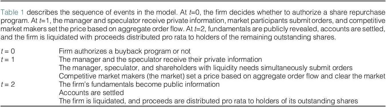
TABLE 1 Long description
Starting at the top, t equals 0 marks the firm’s decision to authorize a buyback program or not. The next section, t equals 1, contains three rows: first, the manager and speculator receive private information; second, the manager, speculator, and shareholders with liquidity needs submit orders simultaneously; third, competitive market makers set a price based on aggregate order flow and clear the market. The final section, t equals 2, also has three rows: first, the firm’s fundamentals become public information; second, accounts are settled; third, the firm is liquidated and proceeds are distributed pro rata to holders of outstanding shares.
The trading equilibrium at
$ t=1 $
 consists of three components: a pricing rule, the speculator’s trading strategy, and the manager’s buyback strategy. In equilibrium, the market sets prices equal to the firm’s expected per-share value at
$ t=2 $
consists of three components: a pricing rule, the speculator’s trading strategy, and the manager’s buyback strategy. In equilibrium, the market sets prices equal to the firm’s expected per-share value at
$ t=2 $
 conditional on aggregate order flow and the anticipated strategies of the other parties. The speculator chooses his trading strategy to maximize expected profits given the pricing rule, the manager’s strategy, and his private information. The manager selects her buyback strategy to maximize a weighted combination of the firm’s stock price at
$ t=1 $
conditional on aggregate order flow and the anticipated strategies of the other parties. The speculator chooses his trading strategy to maximize expected profits given the pricing rule, the manager’s strategy, and his private information. The manager selects her buyback strategy to maximize a weighted combination of the firm’s stock price at
$ t=1 $
 and the per-share value at
$ t=2 $
and the per-share value at
$ t=2 $
 , given the pricing rule, the speculator’s strategy, and her private information.
III. Buybacks and Trading Outcomes
This section analyzes how a stock buyback program affects trading outcomes at
$ t=1 $
 . I begin by characterizing the benchmark trading equilibrium without buybacks (denoted with subscript
$ 0 $
. I begin by characterizing the benchmark trading equilibrium without buybacks (denoted with subscript
$ 0 $
 ):
):
Lemma 1. In the absence of a buyback program, the equilibrium pricing rule is

and the speculator buys
$ x $
 shares if and only if he learns that firm fundamentals are high (
$ A=1 $
shares if and only if he learns that firm fundamentals are high (
$ A=1 $
 ).
).
The results of Lemma 1 follow the standard logic of Kyle-type informed trading frameworks. The presence of noise trading implies that the expected market-clearing price is strictly between
$ 0 $
 and
$ 1 $
and
$ 1 $
 both when
$ A=1 $
both when
$ A=1 $
 and
$ A=0 $
and
$ A=0 $
 . Hence, the speculator strictly prefers to buy upon learning
$ A=1 $
. Hence, the speculator strictly prefers to buy upon learning
$ A=1 $
 and to abstain otherwise. The market makers’ equilibrium pricing rule reflects this trading strategy, increasing with the aggregate order flow.
Lemma 1 implies that the speculator’s expected trading profit (
$ \Pi $
 ) in this benchmark is

As is standard in such informed trading frameworks, the speculator’s expected trading profits increase with his private information (
$ \phi $
 ), the volatility of the firm’s fundamentals (
$ \theta \left(1-\theta \right) $
), the volatility of the firm’s fundamentals (
$ \theta \left(1-\theta \right) $
 ), and the volatility of noise trade (
$ x $
), and the volatility of noise trade (
$ x $
 ). More uncertainty about fundamentals amplifies potential mispricing and, in turn, trading profits. Additional noise trade allows him to take larger positions without revealing his information.
A. Trading Equilibrium with Buybacks
This section analyzes the implications of a buyback program for trading outcomes. The authorization of a buyback program at
$ t=0 $
 makes the firm an active participant in the market for its shares, with the manager effectively becoming another informed trader at
$ t=1 $
makes the firm an active participant in the market for its shares, with the manager effectively becoming another informed trader at
$ t=1 $
 . In this section, I assume that the manager executes buybacks with probability
$ {b}_1=1 $
. In this section, I assume that the manager executes buybacks with probability
$ {b}_1=1 $
 when firm fundamentals are high (
$ A=1 $
when firm fundamentals are high (
$ A=1 $
 ) and with probability
$ {b}_0\in \left[0,1\right] $
) and with probability
$ {b}_0\in \left[0,1\right] $
 when fundamentals are low (
$ A=0 $
when fundamentals are low (
$ A=0 $
 ). Section IV shows that such a buyback strategy is indeed optimal for a manager who maximizes a weighted combination of the firm’s stock price at
$ t=1 $
). Section IV shows that such a buyback strategy is indeed optimal for a manager who maximizes a weighted combination of the firm’s stock price at
$ t=1 $
 and the per-share value at
$ t=2 $
and the per-share value at
$ t=2 $
 .Footnote
14 One interpretation of the buyback strategy is that the manager executes a fraction
$ {b}_0 $
.Footnote
14 One interpretation of the buyback strategy is that the manager executes a fraction
$ {b}_0 $
 of the program in an uninformed manner—buying
$ x $
of the program in an uninformed manner—buying
$ x $
 shares regardless of fundamentals—and the remaining fraction
$ 1-{b}_0 $
shares regardless of fundamentals—and the remaining fraction
$ 1-{b}_0 $
 in an informed manner—buying only when fundamentals are high. Under this interpretation,
$ 1-{b}_0 $
in an informed manner—buying only when fundamentals are high. Under this interpretation,
$ 1-{b}_0 $
 measures the informativeness of buybacks. As
$ {b}_0 $
measures the informativeness of buybacks. As
$ {b}_0 $
 increases, the difference in the execution probabilities in good and bad states narrows, and buybacks become less informative. Buybacks are fully uninformed when
$ {b}_0=1 $
increases, the difference in the execution probabilities in good and bad states narrows, and buybacks become less informative. Buybacks are fully uninformed when
$ {b}_0=1 $
 : the manager buys with the same probability in good and bad states, so buybacks carry no information about fundamentals.
A buyback program changes the trading equilibrium in important ways. The following lemma characterizes the new trading equilibrium with buybacks (denoted with subscript
$ B $
 ):
):
Lemma 2. Given a stock buyback program and the manager’s buyback execution strategy
$ \left({b}_1=1,{b}_0\right) $
 , the equilibrium pricing rule is
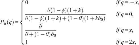
and the speculator buys
$ x $
 shares if and only if he learns that firm fundamentals are high (
$ A=1 $
shares if and only if he learns that firm fundamentals are high (
$ A=1 $
 ).Footnote
15
).Footnote
15
A stock buyback program introduces two economic forces to trading at
$ t=1 $
 . First, it affects the market’s inferences about firm fundamentals by altering the information content of the order flow. This informed execution of buybacks makes the order flow more revealing, improving price discovery and lowering informed trading profits. This competition effect is a robust feature of trading frameworks with multiple informed parties. Second, the program generates buyback profits and losses that make the firm’s per-share value more sensitive to its fundamentals. This dispersion effect is unique to the buyback setting.
1. Competition Effect
A buyback program introduces the firm’s manager as an additional informed trader who may execute buybacks in ways that affect the informativeness of the order flow. To see this clearly, consider how the market updates its beliefs about the firm’s fundamentals (
$ A $
 ) based on the observed order flow (
$ q $
) based on the observed order flow (
$ q $
 ):
$ \hat{\theta}(q)=\mathit{\Pr}\left(A=1|q\right) $
):
$ \hat{\theta}(q)=\mathit{\Pr}\left(A=1|q\right) $
 . In the benchmark without buybacks, the market’s posterior belief is

With buybacks, the market’s posterior belief becomes

One measure of market informativeness is the difference between the market’s expected posterior belief in the two fundamental states:
 . A larger
$ \Delta \hat{\theta} $
. A larger
$ \Delta \hat{\theta} $
 indicates that the order flow better discriminates between high (
$ A=1 $
indicates that the order flow better discriminates between high (
$ A=1 $
 ) and low fundamentals (
$ A=0 $
) and low fundamentals (
$ A=0 $
 ), with
$ \Delta \hat{\theta}=1 $
), with
$ \Delta \hat{\theta}=1 $
 corresponding to the case where the market perfectly infers the firm’s fundamentals from the order flow. Comparing equations (4) and (5) yields the following result:
Lemma 3. Relative to the benchmark, a buyback program improves market informativeness (
$ \Delta {\hat{\theta}}_B>\Delta {\hat{\theta}}_0 $
 ) if buybacks are informed (
$ {b}_0<1 $
) if buybacks are informed (
$ {b}_0<1 $
 ). The improvement increases with buyback informativeness.
When buybacks are uninformed (
$ {b}_0=1 $
 ), they simply shift the distribution of the order flow—increasing it by
$ x $
), they simply shift the distribution of the order flow—increasing it by
$ x $
 —across all fundamental states, as shown in Figure 1. This shift does not affect the information content of the order flow, leaving market informativeness unchanged (
$ \Delta {\hat{\theta}}_B=\Delta {\hat{\theta}}_0 $
—across all fundamental states, as shown in Figure 1. This shift does not affect the information content of the order flow, leaving market informativeness unchanged (
$ \Delta {\hat{\theta}}_B=\Delta {\hat{\theta}}_0 $
 ).
).
The upper portion of Figure 1 shows the distribution of the order flow (
$ q $
 ) across different firm fundamentals (
$ A $
) across different firm fundamentals (
$ A $
 ) in the absence of a buyback program. The lower portion shows how uninformed buybacks (
$ 1-{b}_0=0 $
) in the absence of a buyback program. The lower portion shows how uninformed buybacks (
$ 1-{b}_0=0 $
 ) shift the distribution of the order flow to the right by
$ x $
) shift the distribution of the order flow to the right by
$ x $
 units in all states, leaving the informativeness of the order flow unchanged. Bracketed terms report the probabilities of the corresponding rows.
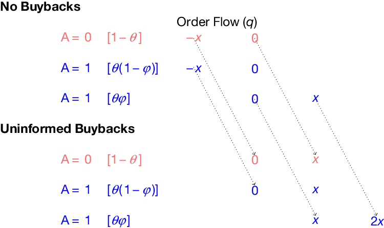
FIGURE 1 Long description
The chart is divided into two horizontal panels. The top panel, labeled No Buybacks, lists three rows for A equals 0 and A equals 1, each with bracketed probabilities in red. For A equals 0, the probability is open bracket 1 minus theta close bracket, and order flow q is negative x or 0. For A equals 1, the first row has probability open bracket theta times open parenthesis 1 minus phi close parenthesis close bracket, and order flow q is negative x or 0. The second A equals 1 row has probability open bracket theta phi close bracket, and order flow q is 0 or x. Dotted lines connect each probability to its corresponding order flow value. The bottom panel, labeled Uninformed Buybacks, repeats the same three rows for A with identical probabilities, but the order flow q values are shifted rightward: for A equals 0, q is 0 or x; for the first A equals 1 row, q is 0 or x; for the second A equals 1 row, q is x or 2 x. Dotted lines again connect each probability to its new order flow values, illustrating a uniform rightward shift in order flow across all states.
In contrast, informed buybacks (
$ 1-{b}_0>0 $
 ) make the order flow more revealing of firm fundamentals. As illustrated in Figure 2, informed buybacks are more likely to shift the order flow distribution rightward when firm fundamentals are high (
$ A=1 $
) make the order flow more revealing of firm fundamentals. As illustrated in Figure 2, informed buybacks are more likely to shift the order flow distribution rightward when firm fundamentals are high (
$ A=1 $
 ) than when they are low (
$ A=0 $
) than when they are low (
$ A=0 $
 ). This state-contingent shift makes high-order flows more indicative of high fundamentals, and low-order flows more indicative of low fundamentals. The more informative the buybacks (i.e., higher
$ 1-{b}_0 $
). This state-contingent shift makes high-order flows more indicative of high fundamentals, and low-order flows more indicative of low fundamentals. The more informative the buybacks (i.e., higher
$ 1-{b}_0 $
 ), the greater the improvement in market informativeness.
The upper portion of Figure 2 shows the distribution of the order flow (
$ q $
 ) across different firm fundamentals (
$ A $
) across different firm fundamentals (
$ A $
 ) in the absence of buybacks. The lower portion illustrates how informed buybacks improve the informativeness of the order flow by shifting the distribution of the order flow to the right more when the firm’s fundamentals are high (
$ A=1 $
) in the absence of buybacks. The lower portion illustrates how informed buybacks improve the informativeness of the order flow by shifting the distribution of the order flow to the right more when the firm’s fundamentals are high (
$ A=1 $
 ) than when they are low (
$ A=0 $
) than when they are low (
$ A=0 $
 ). Bracketed terms report the probabilities of the corresponding rows.
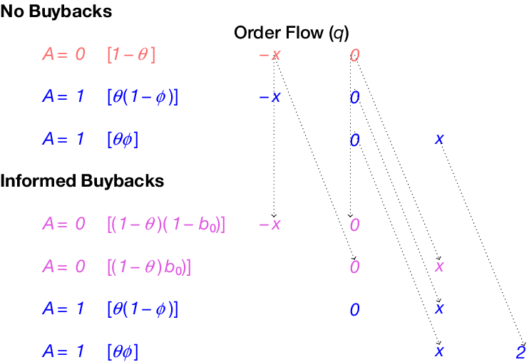
FIGURE 2 Long description
The table is divided into two sections. The upper section, labeled No Buybacks, lists three rows for firm fundamentals: A equals 0 with probability one minus theta, A equals 1 with probability theta times open parenthesis one minus phi close parenthesis, and A equals 1 with probability theta phi. Each row connects by dotted lines to order flow q values: minus x, 0, and x. The lower section, labeled Informed Buybacks, has four rows: A equals 0 with probability open bracket one minus theta close bracket times open bracket one minus b sub 0 close bracket, A equals 0 with probability open bracket one minus theta close bracket b sub 0, A equals 1 with probability theta times open parenthesis one minus phi close parenthesis, and A equals 1 with probability theta phi. These connect to order flow values minus x, 0, x, and 2 x. Dotted lines indicate how probabilities map to order flow outcomes, with more mass shifted to higher order flow values under Informed Buybacks, especially when A equals 1.
Informed buybacks that closely track the firm’s fundamentals erode the speculator’s informational advantage by making the order flow more revealing. In other words, informed buybacks compete against the speculator’s informed trades.
These results parallel the classic literature on competing informed traders (e.g., Admati and Pfleiderer (Reference Admati and Pfleiderer1988), Holden and Subrahmanyam (Reference Holden and Subrahmanyam1992), Foster and Viswanathan (Reference Foster and Viswanathan1993), and Back et al. (Reference Back, Cao and Willard2000)), where additional informed parties enhance price informativeness and compress existing traders’ profits. However, a crucial distinction emerges: in conventional models, informed traders use private accounts and personally bear their trading gains and losses. While their activities alter the firm’s ownership composition, they do not directly affect per-share value.Footnote 16 Consequently, the competition effect completely captures the impact of introducing an additional informed trader.
In my framework, however, the additional informed trader is the manager acting on behalf of the firm. Her buyback trades affect not only the information content of order flow but also the distribution of per-share value through realized trading gains and losses—introducing the novel dispersion effect analyzed next.
2. Dispersion Effect
Buyback activity generates trading gains and losses that accrue to the firm’s remaining shareholders. Consequently, with buybacks, the firm’s per-share value at
$ t=2 $
 becomes
$ V=A+T $
becomes
$ V=A+T $
 , where
$ A $
, where
$ A $
 represents the fundamental payoff from the firm’s assets and
$ T $
represents the fundamental payoff from the firm’s assets and
$ T $
 captures the per-share gains and losses from the firm’s trading activity.
The impact of buybacks on the firm’s per-share value at
$ t=2 $
 depends on whether its shares are under- or overvalued at
$ t=1 $
depends on whether its shares are under- or overvalued at
$ t=1 $
 . When fundamentals are high relative to the market-clearing price at
$ t=1 $
. When fundamentals are high relative to the market-clearing price at
$ t=1 $
 (
$ A>{P}_B $
(
$ A>{P}_B $
 ), the firm buys back undervalued shares, generating trading gains that increase per-share value at
$ t=2 $
), the firm buys back undervalued shares, generating trading gains that increase per-share value at
$ t=2 $
 from
$ A $
from
$ A $
 to
$ {V}_H $
to
$ {V}_H $
 (i.e.,
$ T>0 $
(i.e.,
$ T>0 $
 ):
):

where
$ k=\frac{x}{1-x} $
 is the scale of the buyback program. Conversely, when fundamentals are low relative to the market-clearing price at
$ t=1 $
is the scale of the buyback program. Conversely, when fundamentals are low relative to the market-clearing price at
$ t=1 $
 (
$ A<{P}_B $
(
$ A<{P}_B $
 ), the firm buys back overvalued shares, generating trading losses that decrease per-share value at
$ t=2 $
), the firm buys back overvalued shares, generating trading losses that decrease per-share value at
$ t=2 $
 from
$ A $
from
$ A $
 to
$ {V}_L $
to
$ {V}_L $
 (i.e.,
$ T<0 $
(i.e.,
$ T<0 $
 ):
):

Unlike the trades of speculators, buybacks tend to increase the firm’s per-share value when its fundamentals are high (
$ A=1 $
 ) and decrease the firm’s per-share value when its fundamentals are low (
$ A=0 $
) and decrease the firm’s per-share value when its fundamentals are low (
$ A=0 $
 ). As a result, buybacks amplify the sensitivity of the firm’s per-share value to its fundamentals—the dispersion effect.
Footnote
17
). As a result, buybacks amplify the sensitivity of the firm’s per-share value to its fundamentals—the dispersion effect.
Footnote
17
To quantify this effect, consider the dispersion in the firm’s expected per-share value between good (
$ A=1 $
 ) and bad (
$ A=0 $
) and bad (
$ A=0 $
 ) states:
$ \Delta V=E\left[V|A=1\right]-E\left[V|A=0\right] $
) states:
$ \Delta V=E\left[V|A=1\right]-E\left[V|A=0\right] $
 . In the benchmark without buybacks, this measure simply equals the fundamental spread in asset payoffs:
$ \Delta {V}_0=1 $
. In the benchmark without buybacks, this measure simply equals the fundamental spread in asset payoffs:
$ \Delta {V}_0=1 $
 . With buybacks, the dispersion becomes

where
$ {\overline{T}}_G $
 and
$ {\overline{T}}_L $
and
$ {\overline{T}}_L $
 are the magnitudes of the expected trading gains and losses from executing buybacks when the firm’s fundamentals are high (
$ A=1 $
are the magnitudes of the expected trading gains and losses from executing buybacks when the firm’s fundamentals are high (
$ A=1 $
 ) and low (
$ A=0 $
) and low (
$ A=0 $
 ), respectively.
Lemma 4. Relative to the benchmark, a buyback program strictly increases the dispersion of the firm’s per-share value (
$ \Delta {V}_B>\Delta {V}_0 $
 ). The dispersion in per-share value decreases with the informativeness of buybacks
$ \left(\frac{\mathrm{\partial \Delta }{V}_B}{\partial {b}_0}>0\right) $
). The dispersion in per-share value decreases with the informativeness of buybacks
$ \left(\frac{\mathrm{\partial \Delta }{V}_B}{\partial {b}_0}>0\right) $
 .
.
Buybacks increase the dispersion of the firm’s per-share value: they tend to raise per-share value when fundamentals are high and reduce it when fundamentals are low. Less informed buybacks amplify value dispersion through two channels. First, they incur larger trading losses in bad states (
$ A=0 $
 ), further suppressing value. Second, they make the order flow less informative, which increases the profitability of good-state buybacks, further boosting value in good states (
$ A=1 $
), further suppressing value. Second, they make the order flow less informative, which increases the profitability of good-state buybacks, further boosting value in good states (
$ A=1 $
 ).
).
The competition effect of buybacks improves market informativeness and reduces information asymmetry about the firm’s fundamentals among market participants. The dispersion effect works in the opposite direction—the increased sensitivity of the firm’s per-share value to its fundamentals makes any residual private information more valuable for trading. These changes have important economic consequences, as they determine both the efficiency of market prices and the distribution of trading gains between the speculator and the firm’s shareholders.
B. Speculator’s Profits
This section explores how buybacks shape trading outcomes, focusing on the speculator’s expected trading profits. Because these gains come at the expense of shareholders with liquidity needs, they are essential for evaluating how buybacks affect shareholder welfare.
To begin, consider the following measure of price discovery:
$ \Delta P=\unicode{x1D53C}\left[P|A=1\right]-\unicode{x1D53C}\left[P|A=0\right] $
 . It captures how much market prices differ across fundamental states, with higher values indicating that prices better reflect the firm’s underlying value. In the benchmark without buybacks, price discovery coincides with market informativeness because the firm’s per-share value only depends on the fundamental payoff of its assets (
$ A $
. It captures how much market prices differ across fundamental states, with higher values indicating that prices better reflect the firm’s underlying value. In the benchmark without buybacks, price discovery coincides with market informativeness because the firm’s per-share value only depends on the fundamental payoff of its assets (
$ A $
 ):
$ \Delta {P}_0=\Delta {\hat{\theta}}_0 $
):
$ \Delta {P}_0=\Delta {\hat{\theta}}_0 $
 . With buybacks, price discovery involves learning both about fundamentals and about buyback trading gains, which are jointly determined.
Lemma 5. Price discovery improves with the informativeness of buybacks
$ \left(\frac{\mathrm{\partial \Delta }{P}_B}{\partial {b}_0}<0\right) $
 .
.
At first glance, this result may seem puzzling. The analysis in Section III.A.2 shows that less informed buybacks generate more dispersion in per-share value, suggesting that prices should also diverge more across fundamental states. However, price discovery depends not only on the actual dispersion of per-share value, but also on what the market can infer from the order flow. Section III.A.1 shows that less informed buybacks decrease the information content of the order flow. This effect dominates, and a more informed execution of buybacks improves price discovery.
Recall that
$ {q}_S $
 denotes the speculator’s order. His expected trading profit can be expressed as

where the last equality follows from the market-clearing condition (
$ \unicode{x1D53C}\left[V-P\right]=0 $
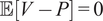 ). The speculator profits to the extent that his trades covary positively with the deviation of per-share value from price—that is, he gains by buying when the firm’s shares are undervalued and abstaining when they are overvalued.
To build intuition, consider the limiting case with
$ \phi \to 1 $
 , where the speculator is almost always informed. Recall that the speculator buys (
$ {q}_S=x $
, where the speculator is almost always informed. Recall that the speculator buys (
$ {q}_S=x $
 ) if and only if he learns that firm fundamentals are high (
$ A=1 $
) if and only if he learns that firm fundamentals are high (
$ A=1 $
 ). In this case, the speculator almost always observes fundamentals, so his order (
$ {q}_S $
). In this case, the speculator almost always observes fundamentals, so his order (
$ {q}_S $
 ) is nearly perfectly correlated with
$ A $
) is nearly perfectly correlated with
$ A $
 , implying that

and

This decomposition in equation (11) reveals the tension between the two effects of buybacks. The competition effect improves price discovery (
$ \Delta {P}_B>\Delta {P}_0 $
 ), compressing the speculator’s informational advantage. The dispersion effect increases the spread in per-share value across fundamental states (
$ \Delta {V}_B>\Delta {V}_0 $
), compressing the speculator’s informational advantage. The dispersion effect increases the spread in per-share value across fundamental states (
$ \Delta {V}_B>\Delta {V}_0 $
 ), making his private information about firm fundamentals more valuable for trading. Buybacks reduce the speculator’s expected trading profit relative to the benchmark if and only if the competition effect dominates the dispersion effect.
In the more general case with
$ \phi \in \left(0,1\right) $
 , the speculator is not always informed. As a result, his trades are not perfectly correlated with firm fundamentals, and the expression for his expected trading profit does not decompose cleanly into value dispersion and price discovery components. Intuitively, what matters is how value and prices vary across the speculator’s trading decisions, not just across fundamental states. Nevertheless, the same economic forces apply: the dispersion effect raises the stakes for informed trading, while the competition effect erodes the speculator’s informational advantage. The following proposition formalizes these results:
Proposition 1. Relative to the benchmark, a buyback program strictly decreases the speculator’s expected trading profit if and only if buybacks are sufficiently informed: there exists a threshold
$ {\overline{b}}_0\in \left(0,1\right) $
 such that
$ {\Pi}_B<{\Pi}_0\iff {b}_0<{\overline{b}}_0 $
such that
$ {\Pi}_B<{\Pi}_0\iff {b}_0<{\overline{b}}_0 $
 .
.
An immediate implication of Proposition 1 is that uninformed buybacks (
$ {b}_0=1 $
 ) unambiguously increase the speculator’s expected trading profits. Uninformed buybacks maximize the dispersion effect while contributing nothing to the competition effect. The speculator benefits from the increased value dispersion without facing any additional competition for trading profits.
The results in this section characterize how buybacks affect the speculator’s expected trading profits, which, in turn, reveal how they affect the aggregate payoffs of the firm’s existing shareholders. For this analysis, the level of informed speculation (
$ \phi $
 ) affects the magnitude of changes but not the qualitative conclusions. However, when analyzing how buybacks affect different types of shareholders, the level of informed speculation becomes qualitatively important as well. Section III.C explores these welfare implications.
C. Heterogeneous Shareholder Welfare
A central concern in the literature is that informed buybacks transfer wealth from outside shareholders to insiders—a phenomenon Fried (Reference Fried2013) calls “insider trading via the firm” (see also Barclay and Smith (Reference Barclay and Smith1988), Fried (Reference Fried2005), Buffa and Nicodano (Reference Buffa and Nicodano2008), and Babenko, Tserlukevich, and Wan (Reference Babenko, Tserlukevich and Wan2020) for similar arguments). The mechanism underlying this wealth transfer is not insider status per se, but rather that insiders typically hold their shares until firm value is realized, whereas outside shareholders may need to sell beforehand to satisfy liquidity needs. Hence, this section examines how a buyback program affects shareholders with different exposures to liquidity shocks.
So far, the analysis has been agnostic about how the firm’s ownership is structured. To connect to the literature on wealth transfers between insiders and outside shareholders, I consider two types of investors who initially own the firm: liquidity-exposed and liquidity-insulated, denoted with superscript
$ E $
 and
$ I $
and
$ I $
 , respectively. Liquidity-exposed shareholders own a fraction
$ x $
, respectively. Liquidity-exposed shareholders own a fraction
$ x $
 of the firm; their liquidity needs at
$ t=1 $
of the firm; their liquidity needs at
$ t=1 $
 are the source of noise trade in the model.Footnote
18 Liquidity-insulated shareholders own the remaining
$ 1-x $
are the source of noise trade in the model.Footnote
18 Liquidity-insulated shareholders own the remaining
$ 1-x $
 shares and hold their position until
$ t=2 $
shares and hold their position until
$ t=2 $
 . These two groups represent the extremes of liquidity exposure. The payoffs of shareholders with intermediate exposures can be obtained as convex combinations of the payoffs of these two groups, providing insight into heterogeneous welfare effects—including for insiders and outside shareholders as conventionally defined.
In the benchmark, the firm’s expected per-share value at
$ t=2 $
 equals
$ \theta $
equals
$ \theta $
 , the expected fundamental payoff of its assets. The expected payoff of liquidity-insulated shareholders is
$ {U}_0^I=\left(1-x\right)\theta $
, the expected fundamental payoff of its assets. The expected payoff of liquidity-insulated shareholders is
$ {U}_0^I=\left(1-x\right)\theta $
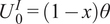 . The expected payoff of liquidity-exposed shareholders is
$ {U}_0^E= x\theta -{\Pi}_0 $
. The expected payoff of liquidity-exposed shareholders is
$ {U}_0^E= x\theta -{\Pi}_0 $
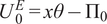 . Because of their liquidity needs at
$ t=1 $
. Because of their liquidity needs at
$ t=1 $
 , the speculator’s trading profits come at their expense.
With buybacks, the firm’s expected per-share value at
$ t=2 $
 becomes
$ \theta +\unicode{x1D53C}\left[T\right] $
becomes
$ \theta +\unicode{x1D53C}\left[T\right] $
 , where
$ \unicode{x1D53C}\left[T\right] $
, where
$ \unicode{x1D53C}\left[T\right] $
 is the expected per-share trading gains of its buyback program. The expected payoff of liquidity-insulated shareholders becomes
$ {U}_B^I=\left(1-x\right)\left(\theta +\unicode{x1D53C}\left[T\right]\right) $
is the expected per-share trading gains of its buyback program. The expected payoff of liquidity-insulated shareholders becomes
$ {U}_B^I=\left(1-x\right)\left(\theta +\unicode{x1D53C}\left[T\right]\right) $
 .
.
Lemma 6. The expected per-share trading gain of the buyback program is positive (
$ \unicode{x1D53C}\left[T\right]\ge 0 $
 ) and increases with the informativeness of buybacks
$ \left(\frac{\partial \unicode{x1D53C}\left[T\right]}{\partial {b}_0}<0\right) $
) and increases with the informativeness of buybacks
$ \left(\frac{\partial \unicode{x1D53C}\left[T\right]}{\partial {b}_0}<0\right) $
 .
.
An informed manager who executes buybacks based on her private information about firm fundamentals earns trading profits in expectation: she is more likely to buy back shares when they are undervalued than when they are overvalued. The more buybacks reflect the manager’s private information, the larger the expected profits from buybacks.
Because the firm’s liquidity-insulated shareholders hold their shares until
$ t=2 $
 , they avoid adverse-selection trading costs at
$ t=1 $
, they avoid adverse-selection trading costs at
$ t=1 $
 . Instead, they benefit from the trading gains generated by informed buybacks. Lemma 6, therefore, implies that liquidity-insulated shareholders are always weakly better off with a buyback program, strictly so if buybacks are informed (
$ {b}_0<1 $
. Instead, they benefit from the trading gains generated by informed buybacks. Lemma 6, therefore, implies that liquidity-insulated shareholders are always weakly better off with a buyback program, strictly so if buybacks are informed (
$ {b}_0<1 $
 ). This result echoes a concern emphasized by Barclay and Smith (Reference Barclay and Smith1988) and others in the literature: informed buybacks benefit those who hold their shares until firm fundamentals are revealed at the expense of those who may need to sell earlier. This traditional perspective implies that liquidity-exposed shareholders prefer less informed buybacks to limit this wealth transfer. Whether this conclusion holds, however, depends on the prevalence of informed speculation (
$ \phi $
). This result echoes a concern emphasized by Barclay and Smith (Reference Barclay and Smith1988) and others in the literature: informed buybacks benefit those who hold their shares until firm fundamentals are revealed at the expense of those who may need to sell earlier. This traditional perspective implies that liquidity-exposed shareholders prefer less informed buybacks to limit this wealth transfer. Whether this conclusion holds, however, depends on the prevalence of informed speculation (
$ \phi $
 ) in the market.
To see why, note that buybacks present a more complex trade-off for liquidity-exposed shareholders because they affect two wealth transfers: one to liquidity-insulated shareholders and another to the speculator. With buybacks, the expected payoff of liquidity-exposed shareholders is

The first term (
$ x\theta $
 ) is the fundamental value of the liquidity-exposed shareholders’ stake. The second term (
$ \left(1-x\right)\unicode{x1D53C}\left[T\right] $
) is the fundamental value of the liquidity-exposed shareholders’ stake. The second term (
$ \left(1-x\right)\unicode{x1D53C}\left[T\right] $
 ) reflects a wealth transfer to liquidity-insulated shareholders, who capture a fraction of the expected buyback gains without incurring trading costs. The final term (
$ {\Pi}_B $
) reflects a wealth transfer to liquidity-insulated shareholders, who capture a fraction of the expected buyback gains without incurring trading costs. The final term (
$ {\Pi}_B $
 ) is the wealth transfer to the speculator, whose informed trades profit at the expense of liquidity-exposed shareholders. One can interpret the last two terms as the reduction in the expected payoff of liquidity-exposed shareholders due to illiquidity.
More informative buybacks have two opposing effects on this payoff. They increase the wealth transfer to liquidity-insulated shareholders, but also decrease the wealth transfer to the speculator. In general, the net effect is ambiguous and can be nonmonotonic.

However, we can characterize the effects when informed speculation (
$ \phi $
 ) is sufficiently rare or sufficiently prevalent. When informed speculation is sufficiently rare, liquidity-exposed shareholders face limited adverse-selection trading costs in the benchmark, so the benefit of reducing the speculator’s profits is small. In this case, the wealth transfer to liquidity-insulated shareholders dominates, and liquidity-exposed shareholders prefer less informative buybacks.
Proposition 2. When informed speculation is sufficiently rare (
$ \phi <\underline{\phi} $
 ), the expected payoff of liquidity-exposed shareholders decreases with the informativeness of buybacks
$ \left(\frac{\partial {U}_B^E}{\partial {b}_0}>0\right) $
), the expected payoff of liquidity-exposed shareholders decreases with the informativeness of buybacks
$ \left(\frac{\partial {U}_B^E}{\partial {b}_0}>0\right) $
 .
.
This result aligns with the conventional view in the literature, which abstracts from informed speculation and concludes that liquidity-exposed shareholders prefer less informed buybacks to limit the wealth transfer to liquidity-insulated shareholders, such as insiders. Proposition 2 shows that this conclusion holds when informed speculation is sufficiently rare—including the limiting case of
$ \phi \to 0 $
 implicitly assumed in many prior studies.
When informed speculation is sufficiently prevalent, the opposite can occur. Liquidity-exposed shareholders face substantial adverse-selection costs in the benchmark, so the benefit from reduced speculator profits can more than offset the wealth transfer to liquidity-insulated shareholders.
Proposition 3. When informed speculation is sufficiently prevalent (
$ \phi >\overline{\phi} $
 ), the expected payoff of liquidity-exposed shareholders increases with the informativeness of buybacks
$ \left(\frac{\partial {U}_B^E}{\partial {b}_0}<0\right) $
), the expected payoff of liquidity-exposed shareholders increases with the informativeness of buybacks
$ \left(\frac{\partial {U}_B^E}{\partial {b}_0}<0\right) $
 .
.
Proposition 3 suggests that the firm can use informed buybacks to protect its liquidity-exposed shareholders from adverse-selection trading costs, consistent with the findings of Wiggins (Reference Wiggins1994), who documents that the adverse-selection component of the bid–ask spread tends to widen before the authorization of a buyback program and narrow afterward. More recently, Hillert, Maug, and Obernberger (Reference Hillert, Maug and Obernberger2016) conclude that “the information content of repurchases is not associated with a deterioration of liquidity […] higher information content seems to be associated with improvements and not with deterioration in liquidity at the time repurchases were executed.”
The preceding analysis might suggest that uninformed buybacks are benign—they minimize wealth transfers to insiders while avoiding the complications of informed execution. They are not:
Corollary 1. Relative to the benchmark without buybacks (Lemma 1), a buyback program strictly lowers the expected payoff of the firm’s liquidity-exposed shareholders when buybacks are uninformed (
$ {b}_0=1 $
 ) and informed speculation is present (
$ \phi >0 $
) and informed speculation is present (
$ \phi >0 $
 ).
).
At first glance, Corollary 1 may seem puzzling. Uninformed buybacks—which are always executed regardless of firm fundamentals—neither make nor lose money in expectation. Why should they harm liquidity-exposed shareholders?
The crux of the result is that the speculator’s informed trading induces a correlation between the liquidity trades of liquidity-exposed shareholders and the profitability of buybacks. The presence of informed speculative trading (
$ \phi >0 $
 ) results in an equilibrium pricing rule that increases with order flow even when buybacks are uninformed. When liquidity-exposed shareholders sell to meet liquidity needs, they simultaneously reduce their stake in the firm and push down the price at which buybacks are executed. Consequently, they are less likely to retain shares in states where buybacks generate gains. Even though uninformed buybacks break even in expectation, liquidity-exposed shareholders receive a disproportionately small share of the gains and bear a disproportionately large share of the losses. This correlation causes liquidity-exposed shareholders to incur net losses from uninformed buybacks. Such a channel is absent in conventional models without buybacks, where informed speculation affects only the price at which liquidity-exposed shareholders sell, not the per-share value of the shares they retain.
The stock buyback literature often emphasizes how informed buybacks can hurt liquidity-exposed shareholders (e.g., Barclay and Smith (Reference Barclay and Smith1988), Brockman and Chung (Reference Brockman and Chung2001), Buffa and Nicodano (Reference Buffa and Nicodano2008), Fried (Reference Fried2013), and Babenko et al. (Reference Babenko, Tserlukevich and Wan2020)). This conventional view suggests that firms could protect them by committing not to use the manager’s private information when executing buybacks. The analysis in this section shows that this view is incomplete. While informed buybacks do transfer wealth to liquidity-insulated shareholders, uninformed buybacks are not a neutral alternative. They subject liquidity-exposed shareholders to additional adverse-selection costs arising from the speculator’s informed trades. In fact, when informed speculation is sufficiently prevalent, informed buybacks can actually benefit liquidity-exposed shareholders by reducing the speculator’s profits (Proposition 3). The desirability of informed versus uninformed buybacks thus depends critically on the level of informed speculation already present in the market.
IV. Manager’s Buyback Strategy
This section examines the optimal buyback strategy of a manager who maximizes
$ \unicode{x1D53C}\left[\omega P+V\right] $
 , where
$ P $
, where
$ P $
 is the firm’s stock price at
$ t=1 $
is the firm’s stock price at
$ t=1 $
 ,
$ V $
,
$ V $
 is the firm’s per-share value at
$ t=2 $
is the firm’s per-share value at
$ t=2 $
 , and
$ \omega \ge 0 $
, and
$ \omega \ge 0 $
 captures her concern for the firm’s interim stock price. When
$ \omega =0 $
captures her concern for the firm’s interim stock price. When
$ \omega =0 $
 , the manager only cares about the firm’s per-share value at
$ t=2 $
, the manager only cares about the firm’s per-share value at
$ t=2 $
 . As
$ \omega $
. As
$ \omega $
 increases, she places greater emphasis on the interim stock price. In the limiting case as
$ \omega \to \infty $
increases, she places greater emphasis on the interim stock price. In the limiting case as
$ \omega \to \infty $
 , her objective is driven entirely by the interim stock price.
Recall that the manager’s buyback strategy specifies the probability with which she executes buybacks when firm fundamentals are high (
$ {b}_1 $
 ) and when they are low (
$ {b}_0 $
) and when they are low (
$ {b}_0 $
 ). When firm fundamentals are high (
$ A=1 $
). When firm fundamentals are high (
$ A=1 $
 ), executing buybacks is a dominant strategy for the manager. Buying back
$ x $
), executing buybacks is a dominant strategy for the manager. Buying back
$ x $
 shares strictly increases the expected market-clearing stock price at
$ t=1 $
shares strictly increases the expected market-clearing stock price at
$ t=1 $
 and generates trading profits that raise the per-share value at
$ t=2 $
and generates trading profits that raise the per-share value at
$ t=2 $
 . Hence, when the manager learns that firm fundamentals are high, she executes buybacks with certainty (
$ {b}_1^{\ast }=1 $
. Hence, when the manager learns that firm fundamentals are high, she executes buybacks with certainty (
$ {b}_1^{\ast }=1 $
 ).
).
However, when firm fundamentals are low (
$ A=0 $
 ), the manager faces a trade-off. Executing buybacks increases the expected market-clearing stock price at
$ t=1 $
), the manager faces a trade-off. Executing buybacks increases the expected market-clearing stock price at
$ t=1 $
 —because the equilibrium pricing rule is increasing in order flow—but generates trading losses that reduce per-share value at
$ t=2 $
—because the equilibrium pricing rule is increasing in order flow—but generates trading losses that reduce per-share value at
$ t=2 $
 . The optimal buyback strategy depends on her concern about the interim stock price (
$ \omega $
. The optimal buyback strategy depends on her concern about the interim stock price (
$ \omega $
 ):
):
Proposition 4. Upon learning that firm fundamentals are high, the manager executes buybacks with certainty (
$ {b}_1^{\ast }=1 $
 ). Upon learning that firm fundamentals are low, she executes buybacks with probability
$ {b}_0^{\ast } $
). Upon learning that firm fundamentals are low, she executes buybacks with probability
$ {b}_0^{\ast } $
 :
:

where
$ 0<\underline{\omega}<\overline{\omega} $
 .Footnote
19
.Footnote
19
When the manager places little weight on the interim stock price (
$ \omega <\underline{\omega} $
 ), she never buys back overvalued shares. For intermediate values (
$ \omega \in \left[\underline{\omega},\overline{\omega}\right] $
), she never buys back overvalued shares. For intermediate values (
$ \omega \in \left[\underline{\omega},\overline{\omega}\right] $
 ), the probability of buyback execution increases continuously with
$ \omega $
), the probability of buyback execution increases continuously with
$ \omega $
 as the manager becomes increasingly inclined to inflate the stock price by buying back overvalued shares. When her concerns about the interim stock price are strong (
$ \omega >\overline{\omega} $
as the manager becomes increasingly inclined to inflate the stock price by buying back overvalued shares. When her concerns about the interim stock price are strong (
$ \omega >\overline{\omega} $
 ), she buys back shares regardless of firm fundamentals. Figure 3 illustrates this relationship. These predictions align with the evidence that managers facing stronger short-term incentives execute more value-destroying buybacks (e.g., Cheng, Harford, and Zhang (Reference Cheng, Harford and Zhang2015), Almeida, Fos, and Kronlund (Reference Almeida, Fos and Kronlund2016), and Edmans, Fang, and Huang (Reference Edmans, Fang and Huang2022)).
Proposition 5. The informativeness of buybacks increases with expected fundamentals (
$ \theta $
 ) and the scale of the buyback program (
$ k $
) and the scale of the buyback program (
$ k $
 ), and decreases with the prevalence of informed speculation (
$ \phi $
), and decreases with the prevalence of informed speculation (
$ \phi $
 ).
).
Figure 3 illustrates the relationship between the manager’s optimal buyback decision and her concern for the interim stock price. For low
$ \omega <\underline{\omega} $
 , the manager never executes the buyback, for intermediate
$ \omega \in \left[\underline{\omega},\overline{\omega}\right] $
, the manager never executes the buyback, for intermediate
$ \omega \in \left[\underline{\omega},\overline{\omega}\right] $
 , she executes with an interior probability, and for high
$ \omega >\overline{\omega} $
, she executes with an interior probability, and for high
$ \omega >\overline{\omega} $
 , she executes the buyback with certainty. Hence, the informativeness of buybacks worsens with
$ \omega $
, she executes the buyback with certainty. Hence, the informativeness of buybacks worsens with
$ \omega $
 .
.
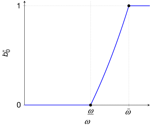
FIGURE 3 Long description
The line graph plots b sub 0 super star on the vertical axis from zero to one and omega on the horizontal axis. The curve starts at zero, remains flat until underlined omega, then increases smoothly between underlined omega and overlined omega, reaching one at overlined omega, and stays flat at one beyond this point. Both underlined omega and overlined omega are marked with black dots and vertical dashed lines. The axes are labeled with b sub 0 super star and omega, with the curve drawn in blue.
Firm characteristics and market conditions affect the manager’s buyback strategy by shaping the costs and benefits of buying back overvalued shares. A higher expected value of firm fundamentals (
$ \theta $
 ) raises the expected stock price, increasing the losses from buying back overvalued shares. Similarly, a larger buyback program (
$ k $
) raises the expected stock price, increasing the losses from buying back overvalued shares. Similarly, a larger buyback program (
$ k $
 ) amplifies the per-share trading losses of buybacks in low-fundamental states. Both effects make the manager less willing to execute buybacks when firm fundamentals are low, increasing the informativeness of buybacks. In contrast, when informed speculation (
$ \phi $
) amplifies the per-share trading losses of buybacks in low-fundamental states. Both effects make the manager less willing to execute buybacks when firm fundamentals are low, increasing the informativeness of buybacks. In contrast, when informed speculation (
$ \phi $
 ) is more prevalent, the pricing rule responds more sharply to order flow, making it easier for the manager to inflate the interim stock price by buying back overvalued shares—thereby reducing the informativeness of buybacks.
When shareholders anticipate the manager’s equilibrium strategy, they can infer the informativeness of buybacks from firm characteristics and market conditions. The next section examines when they would benefit from authorizing a buyback program.
V. Buyback Authorization
This section examines when shareholders would authorize a buyback program at
$ t=0 $
 . Because the authorization precedes the arrival of private information, shareholders form expectations about how the manager will execute buybacks. Proposition 4 establishes that the manager’s equilibrium buyback strategy—and hence the anticipated informativeness of buybacks—depends on her concern about the interim stock price (
$ \omega $
. Because the authorization precedes the arrival of private information, shareholders form expectations about how the manager will execute buybacks. Proposition 4 establishes that the manager’s equilibrium buyback strategy—and hence the anticipated informativeness of buybacks—depends on her concern about the interim stock price (
$ \omega $
 ), firm characteristics (
$ \theta $
), firm characteristics (
$ \theta $
 ), and market conditions (
$ x,\phi $
), and market conditions (
$ x,\phi $
 ). Because shareholders with different liquidity exposures do not benefit equally from buybacks, the authorization decision depends on the firm’s ownership composition and governance structure.
This analysis distinguishes between outside shareholders and insiders, who own fractions
$ s\ge x $
 and
$ 1-s $
and
$ 1-s $
 of the firm, respectively.Footnote
20 Outside shareholders may experience liquidity needs that force them to sell
$ x $
of the firm, respectively.Footnote
20 Outside shareholders may experience liquidity needs that force them to sell
$ x $
 shares at
$ t=1 $
shares at
$ t=1 $
 . In contrast, insiders—such as managers, directors, and blockholders with stable positions—are liquidity-insulated, holding their shares until
$ t=2 $
. In contrast, insiders—such as managers, directors, and blockholders with stable positions—are liquidity-insulated, holding their shares until
$ t=2 $
 with certainty. Using the payoffs derived in Section III.C, the expected payoffs of outside shareholders and insiders are

and

where the scaling reflects that
$ {U}^I $
 is the payoff to the
$ 1-x $
is the payoff to the
$ 1-x $
 liquidity-insulated shares. When
$ s=x $
liquidity-insulated shares. When
$ s=x $
 , outside shareholders are fully exposed to liquidity shocks. When
$ s>x $
, outside shareholders are fully exposed to liquidity shocks. When
$ s>x $
 , they retain some shares until
$ t=2 $
, they retain some shares until
$ t=2 $
 with certainty, and partially benefit from buyback trading gains.
I consider three governance structures that differ in whose interests the board represents in authorizing a buyback program at
$ t=0 $
 . The first is an insider-aligned board that maximizes insider payoffs. The second maximizes the aggregate payoff of existing shareholders at
$ t=2 $
. The first is an insider-aligned board that maximizes insider payoffs. The second maximizes the aggregate payoff of existing shareholders at
$ t=2 $
 . The third weighs shareholder interests in proportion to ownership.
A. Insider-Aligned Board
Because the buyback program generates weakly positive expected trading gains (Lemma 6), insiders benefit from buybacks. Hence, an insider-aligned board always authorizes, implying that restrictions on authorization come from outside shareholder influence.
B. Aggregate Payoff Maximization
Suppose the board maximizes the aggregate payoff of all existing shareholders. Proposition 1 implies a cutoff rule: authorize if and only if buybacks are anticipated to be sufficiently informed (
$ {b}_0^{\ast }<{\overline{b}}_0 $
 ). Proposition 5 then suggests that authorization is more likely when expected firm fundamentals (
$ \theta $
). Proposition 5 then suggests that authorization is more likely when expected firm fundamentals (
$ \theta $
 ) are higher, informed speculation (
$ \phi $
) are higher, informed speculation (
$ \phi $
 ) is less prevalent, and market conditions support larger buyback programs (
$ k $
) is less prevalent, and market conditions support larger buyback programs (
$ k $
 ).
).
The intuition follows from the manager’s execution incentives. Higher expected fundamentals and larger programs make bad-state buybacks more costly, increasing the anticipated informativeness of buybacks. Greater liquidity (lower
$ \phi $
 ) reduces the price impact of order flow, limiting the manager’s ability to inflate the interim stock price with bad-state buybacks. These factors increase the likelihood that the anticipated informativeness of buybacks exceeds the authorization threshold.
These predictions align with documented patterns of buyback activity. The procyclical nature of authorizations, as documented by Jagannathan, Stephens, and Weisbach (Reference Jagannathan, Stephens and Weisbach2000) and Dittmar and Dittmar (Reference Dittmar and Dittmar2008), is consistent with firms authorizing when expected fundamentals are high. Notably, this prediction concerns ex ante expectations at the time of authorization, not ex post realizations—firms authorize when they expect fundamentals to be strong, which differs from the undervaluation hypothesis that firms repurchase when they believe their stock is currently underpriced. The empirical finding that firms with more liquid shares are more likely to authorize buyback programs (Brockman, Howe, and Mortal (Reference Brockman, Howe and Mortal2008)) is consistent with the liquidity prediction.
C. Proportional Representation
Suppose the board authorizes a buyback program if the proportion of the firm’s existing shareholders who benefit exceeds a threshold
$ \tau \in \left(0,1\right) $
 . For instance, the majority rule corresponds to a threshold of
$ \tau =0.5 $
. For instance, the majority rule corresponds to a threshold of
$ \tau =0.5 $
 . The authorization decision then depends on ownership composition (
$ s $
. The authorization decision then depends on ownership composition (
$ s $
 ), the prevalence of informed speculation (
$ \phi $
), the prevalence of informed speculation (
$ \phi $
 ), and the anticipated informativeness of buybacks (
$ {b}_0^{\ast } $
), and the anticipated informativeness of buybacks (
$ {b}_0^{\ast } $
 ).
).
When outside shareholder ownership is low (
$ s<\tau $
 ), insiders determine the outcome. Here, the authorization follows the insider-aligned case, so the board authorizes the buyback program.
When outside shareholder ownership is high (
$ s\ge \tau $
 ), their preferences become pivotal. If informed speculation is rare, outside shareholders lose from any buyback program. Uninformed buybacks amplify adverse-selection costs, increasing the wealth transfer to the speculator. Informed buybacks are even worse—the wealth transfer to insiders dominates the reduction in speculator profits. Authorization fails when informed speculation is sufficiently rare, as both uninformed and informed buybacks harm outside shareholders in this case.Footnote
21
), their preferences become pivotal. If informed speculation is rare, outside shareholders lose from any buyback program. Uninformed buybacks amplify adverse-selection costs, increasing the wealth transfer to the speculator. Informed buybacks are even worse—the wealth transfer to insiders dominates the reduction in speculator profits. Authorization fails when informed speculation is sufficiently rare, as both uninformed and informed buybacks harm outside shareholders in this case.Footnote
21
If informed speculation is prevalent, the situation is more nuanced. Uninformed buybacks remain harmful—and are, in fact, more damaging because the wealth transfer to the speculator is larger. However, sufficiently informed buybacks can benefit outside shareholders: the reduction in speculator profits offsets the wealth transfer to insiders.Footnote
22 Authorization passes if anticipated execution is sufficiently informed. There is a subtle tension: more prevalent informed speculation (higher
$ \phi $
 ) makes reducing the speculator’s trading profits more valuable to outside shareholders—but simultaneously reduces buyback informativeness (Proposition 5), thereby weakening the competition effect that delivers this reduction.
When informed speculation is rare, firms with dispersed ownership face a conflict: insiders prefer authorization, but outside shareholders—who may constitute the majority—are harmed by any buyback program. This conflict can lead to two types of inefficiency. Insiders may push through authorization over outside shareholders’ objections, transferring wealth to themselves without providing offsetting benefits for outside shareholders. Outside shareholders may block authorization, forgoing informed buybacks that would have increased aggregate shareholder payoffs. When informed speculation is prevalent, this tension eases: outside shareholders can benefit from sufficiently informed buybacks, aligning their preferences with insiders. The welfare implications of buyback authorization thus depend not only on governance, but also on market conditions that determine how buybacks are executed.
VI. Model Extensions and Applications
A. Buyback Disclosure
The baseline model assumes that the market only observes the aggregate order flow. In practice, however, regulators have sought to expand the disclosure requirements of buyback activity. For instance, in 2004, the SEC began requiring firms to report monthly buyback activity in their quarterly filings. In 2023, the SEC adopted rules mandating reports of daily buyback activity, though these rules were subsequently vacated by the courts. The policy rationale for enhanced disclosure centers on the adverse-selection problem: insiders may use the manager’s informational advantage to execute buybacks in a way that transfers wealth from outside shareholders to themselves.
This section analyzes how buyback disclosures affect the trading equilibrium. Specifically, I assume that the market observes both the aggregate order flow (
$ q $
 ) and the firm’s buyback order (
$ {q}_B $
) and the firm’s buyback order (
$ {q}_B $
 ) before setting prices—a scenario I refer to as the pretrade buyback disclosure regime (denoted with superscript
$ D $
) before setting prices—a scenario I refer to as the pretrade buyback disclosure regime (denoted with superscript
$ D $
 ). The speculator does not observe the firm’s buyback order prior to submitting his order. As in Section III.A, I assume that the manager’s buyback strategy is (
$ 1,{b}_0 $
). The speculator does not observe the firm’s buyback order prior to submitting his order. As in Section III.A, I assume that the manager’s buyback strategy is (
$ 1,{b}_0 $
 ).Footnote
23
).Footnote
23
Let
$ {\theta}_x $
 and
$ {\theta}_0 $
and
$ {\theta}_0 $
 be the market’s posterior belief about firm fundamentals conditional on observing
$ {q}_B=x $
be the market’s posterior belief about firm fundamentals conditional on observing
$ {q}_B=x $
 and
$ {q}_B=0 $
and
$ {q}_B=0 $
 , respectively. Because the manager always executes buybacks when firm fundamentals are high, the absence of disclosed buybacks (
$ {q}_B=0 $
, respectively. Because the manager always executes buybacks when firm fundamentals are high, the absence of disclosed buybacks (
$ {q}_B=0 $
 ) fully reveals that firm fundamentals are low:
$ {\theta}_0=0 $
) fully reveals that firm fundamentals are low:
$ {\theta}_0=0 $
 . In this case, the market-clearing price equals zero for all order flows.
In contrast, the disclosure of buybacks (
$ {q}_B=x $
 ) indicates that firm fundamentals are more likely to be high:
$ {\theta}_x=\frac{\theta }{\theta +\left(1-\theta \right){b}_0}\ge \theta $
) indicates that firm fundamentals are more likely to be high:
$ {\theta}_x=\frac{\theta }{\theta +\left(1-\theta \right){b}_0}\ge \theta $
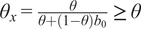 , strictly so when buybacks are informed (
$ {b}_0<1 $
, strictly so when buybacks are informed (
$ {b}_0<1 $
 ). In this case, the trading equilibrium is isomorphic to the one characterized in Lemma 2, with
$ {\theta}_x $
). In this case, the trading equilibrium is isomorphic to the one characterized in Lemma 2, with
$ {\theta}_x $
 replacing
$ \theta $
replacing
$ \theta $
 and buybacks occurring with certainty. Hence, given buybacks (
$ {q}_B=x $
and buybacks occurring with certainty. Hence, given buybacks (
$ {q}_B=x $
 ), the equilibrium pricing rule is

As before, the speculator buys
$ x $
 shares if and only if he learns that firm fundamentals are high (A = 1).
Lemma 7. Pretrade disclosure eliminates expected buyback trading profits (
 ).
).
With pretrade disclosure, the market always observes whether buybacks are occurring. As a result, the manager has no informational advantage vis-à-vis the market, and the buyback program cannot generate positive expected trading profits. Lemma 7 implies that pretrade buyback disclosure eliminates the wealth transfer from outside shareholders to insiders studied in Section III.C. This result is consistent with arguments in the literature that pretrade disclosure prevents insiders from profiting at the expense of outside shareholders (e.g., Fried (Reference Fried2005)).
However, this analysis is incomplete in the presence of informed speculative trading (
$ \phi >0 $
 ). Lemma 4 establishes that buybacks also induce a dispersion effect that increases the value of any remaining informational advantage held by the speculator. As a result, even with pretrade disclosure, the economic consequences of buybacks still depend on their informativeness:
Proposition 6. Under pretrade disclosure, a buyback program decreases the speculator’s expected trading profit relative to the benchmark if and only if buybacks are sufficiently informed.
Buybacks continue to generate two opposing effects in the pretrade buyback disclosure regime. First, buybacks convey information to the market—though under this regime, information transmission occurs directly through disclosure rather than indirectly through order flow. This competition effect erodes the speculator’s informational advantage. Second, buybacks increase the dispersion in per-share value across fundamental states. This dispersion effect makes the speculator’s private information more valuable for trading. Consequently, buybacks decrease the speculator’s expected trading profit if and only if they are sufficiently informed.
Because disclosure eliminates the wealth transfer to insiders, the expected payoff of the firm’s outside shareholders depends solely on the transfer to the speculator:
$ {U}_B^{DO}= x\theta -{\Pi}_B^D $
 . Consequently, they strictly prefer more informed buybacks:
$ \frac{\partial {U}_B^{DO}}{\partial {b}_0}=-\frac{\partial {\Pi}_B^D}{\partial {b}_0}<0 $
. Consequently, they strictly prefer more informed buybacks:
$ \frac{\partial {U}_B^{DO}}{\partial {b}_0}=-\frac{\partial {\Pi}_B^D}{\partial {b}_0}<0 $
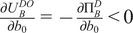 .
.
Thus far, I have taken the manager’s strategy as given. The following demonstrates that the pretrade disclosure regime also affects the manager’s optimal buyback strategy:
Proposition 7. The pretrade buyback disclosure regime makes the manager’s optimal buyback strategy less informed relative to the baseline model.
The crux of Proposition 7 is that pretrade disclosure increases the sensitivity of the interim stock price to buybacks. If the manager does not buy back shares, the market infers that firm fundamentals are low (
$ A=0 $
 ), and the stock price falls. Hence, she faces stronger incentives to execute buybacks when firm fundamentals are low, resulting in a less informed buyback strategy.
These results have nuanced policy implications. Pretrade disclosure eliminates wealth transfers from outside shareholders to insiders, but it does not eliminate the speculator’s trading profits. Outside shareholders, therefore, still prefer more informed buybacks to limit their losses to the speculator. However, disclosure itself reduces the informativeness of buybacks: by punishing nonexecution—the market infers low fundamentals when no buyback is disclosed—the regime strengthens the manager’s incentive to buy back overvalued shares. The net effect of mandatory disclosure on outside shareholder welfare, therefore, depends on whether the benefit of eliminating the wealth transfer to insiders outweighs the cost of reduced buyback informativeness.
B. Other Frictions Affecting Buyback Strategy
The baseline model assumes that the manager executes buybacks to maximize
$ \unicode{x1D53C}\left[\omega P+V\right] $
 , a weighted combination of the firm’s
$ t=1 $
, a weighted combination of the firm’s
$ t=1 $
 stock price (
$ P $
stock price (
$ P $
 ) and its
$ t=2 $
) and its
$ t=2 $
 per-share value (
$ V $
per-share value (
$ V $
 ). Under this objective, the manager always executes buybacks when she learns that fundamentals are high (
$ A=1 $
). Under this objective, the manager always executes buybacks when she learns that fundamentals are high (
$ A=1 $
 ) because doing so strictly increases both the stock price and per-share value. Because the manager is perfectly informed about firm fundamentals and faces no additional constraints, she executes good-state buybacks with certainty.
However, many frictions can prevent the manager from executing buybacks when fundamentals are high. The manager may have imperfect information about fundamentals, limiting her ability to identify good states. Financing constraints may leave the manager without the resources to buy back shares. Regulatory constraints and blackout periods may restrict trading windows. This section extends the analysis of Section III.A to accommodate these possibilities, characterizing equilibrium outcomes for a more general buyback strategy (
$ {b}_1,{b}_0 $
 ), with
$ {b}_1\ge {b}_0 $
), with
$ {b}_1\ge {b}_0 $
 .Footnote
24
.Footnote
24
Here, the manager does not always buy back shares when firm fundamentals are high (
$ {b}_1<1 $
 ). As a result, informativeness has two dimensions: the probability of good-state buybacks (
$ {b}_1 $
). As a result, informativeness has two dimensions: the probability of good-state buybacks (
$ {b}_1 $
 ) and the probability of bad-state buybacks (
$ {b}_0 $
) and the probability of bad-state buybacks (
$ {b}_0 $
 ). For a given
$ {b}_0 $
). For a given
$ {b}_0 $
 , increasing
$ {b}_1 $
, increasing
$ {b}_1 $
 increases informativeness; for a given
$ {b}_1 $
increases informativeness; for a given
$ {b}_1 $
 , decreasing
$ {b}_0 $
, decreasing
$ {b}_0 $
 increases informativeness. The baseline model fixes
$ {b}_1=1 $
increases informativeness. The baseline model fixes
$ {b}_1=1 $
 and captures informativeness by varying
$ {b}_0 $
and captures informativeness by varying
$ {b}_0 $
 :
:
Lemma 8. The manager’s buyback strategy
$ \left({b}_1,{b}_0\right) $
 determines the competitive impact of buybacks through market informativeness:
-
1. More informed buybacks improve market informativeness $ \left(\frac{\mathrm{\partial \Delta }{\hat{\theta}}_B}{\partial {b}_1}>0\hskip0.84em and\frac{\mathrm{\partial \Delta }{\hat{\theta}}_B}{\partial {b}_0}<0\right) $
 .
. -
2. A buyback program improves market informativeness relative to the benchmark ( $ \Delta {\hat{\theta}}_B>\Delta {\hat{\theta}}_0 $
) if and only if buybacks are sufficiently informed:-
• For $ {b}_1>0 $
, there exists a
$ {\underline{b}}_0\in \left(0,{b}_1\right) $
such that
$ \Delta {\hat{\theta}}_B>\Delta {\hat{\theta}}_0\iff {b}_0<{\underline{b}}_0 $
. -
• For $ {b}_0<1 $
, there exists a
$ {\underline{b}}_1\in \left({b}_0,1\right) $
such that
$ \Delta {\hat{\theta}}_B>\Delta {\hat{\theta}}_0\iff {b}_1>{\underline{b}}_1 $
.
-
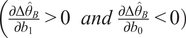






The results in Lemma 8 follow from how the buyback strategy shapes market inferences. When the manager buys more aggressively in good states (higher
$ {b}_1 $
 ), large positive order flows become stronger signals of high firm fundamentals (
$ A=1 $
), large positive order flows become stronger signals of high firm fundamentals (
$ A=1 $
 ). Conversely, when she buys more in bad states (higher
$ {b}_0 $
). Conversely, when she buys more in bad states (higher
$ {b}_0 $
 ), she adds noise that makes large positive order flows less indicative of high firm fundamentals. As in the baseline model, Lemma 8 implies that uninformed buybacks (
$ {b}_1={b}_0=b $
), she adds noise that makes large positive order flows less indicative of high firm fundamentals. As in the baseline model, Lemma 8 implies that uninformed buybacks (
$ {b}_1={b}_0=b $
 ) weakly decrease market informativeness, strictly so if
$ b<1 $
) weakly decrease market informativeness, strictly so if
$ b<1 $
 . Effectively, uninformed buybacks inject additional noise into trading without improving the information contained in order flows.
The dispersion effect is more nuanced in this setting. Recall that the dispersion in the firm’s expected per-share value between good (
$ A=1 $
 ) and bad (
$ A=0 $
) and bad (
$ A=0 $
 ) states is given by
$ \Delta V=E\left[V|A=1\right]-E\left[V|A=0\right] $
) states is given by
$ \Delta V=E\left[V|A=1\right]-E\left[V|A=0\right] $
 . In the benchmark without buybacks, this dispersion simply equals the fundamental spread in asset payoffs:
$ \Delta {V}_0=1 $
. In the benchmark without buybacks, this dispersion simply equals the fundamental spread in asset payoffs:
$ \Delta {V}_0=1 $
 . With buybacks, the dispersion becomes

where
$ {\overline{T}}_G $
 and
$ {\overline{T}}_L $
and
$ {\overline{T}}_L $
 are the magnitudes of the expected trading gains and losses from executing buybacks when the firm’s fundamentals are high (
$ A=1 $
are the magnitudes of the expected trading gains and losses from executing buybacks when the firm’s fundamentals are high (
$ A=1 $
 ) and low (
$ A=0 $
) and low (
$ A=0 $
 ).
).
The buyback strategy (
$ {b}_0,{b}_1 $
 ) affects the dispersion through two channels: a direct trading channel and an indirect spillover channel. The following decomposition reveals an asymmetry—dispersion unambiguously increases with bad-state buybacks but can either increase or decrease with good-state buybacks:

and

More bad-state buybacks (higher
$ {b}_0 $
 ) increase dispersion through both the direct trading and the indirect spillover channels. First, they deepen expected buyback losses, reducing per-share value when fundamentals are weak. Second, they make the order flow less informative, lowering the expected market-clearing price in good states (
$ A=1 $
) increase dispersion through both the direct trading and the indirect spillover channels. First, they deepen expected buyback losses, reducing per-share value when fundamentals are weak. Second, they make the order flow less informative, lowering the expected market-clearing price in good states (
$ A=1 $
 ) and increasing the profitability of good-state buybacks (
$ {\overline{T}}_G $
) and increasing the profitability of good-state buybacks (
$ {\overline{T}}_G $
 ). Consequently, bad-state buybacks unambiguously increase dispersion.
In contrast, more buybacks in good states (higher
$ {b}_1 $
 ) have a more nuanced effect on dispersion. The direct trading channel works as before—good-state buybacks expand expected gains, enhancing per-share value when firm fundamentals are high and increasing dispersion. However, the indirect spillover channel now features a countervailing force—good-state buybacks make the order flow more informative, lowering the expected market-clearing price in bad states and limiting the losses from bad-state buybacks (
$ {\overline{T}}_L $
) have a more nuanced effect on dispersion. The direct trading channel works as before—good-state buybacks expand expected gains, enhancing per-share value when firm fundamentals are high and increasing dispersion. However, the indirect spillover channel now features a countervailing force—good-state buybacks make the order flow more informative, lowering the expected market-clearing price in bad states and limiting the losses from bad-state buybacks (
$ {\overline{T}}_L $
 ). The trading channel dominates when the buyback program size is large (high
$ k $
). The trading channel dominates when the buyback program size is large (high
$ k $
 )—increasing expected trading profits—or when bad-state buybacks are rare (low
$ {b}_0 $
)—increasing expected trading profits—or when bad-state buybacks are rare (low
$ {b}_0 $
 )—making the spillover effect less relevant:
Lemma 9. A buyback program strictly increases the dispersion of the firm’s per-share value across good and bad states (
$ \Delta {V}_B>\Delta {V}_0 $
 ). The magnitude of this effect depends on the execution strategy (
$ {b}_0,{b}_1 $
). The magnitude of this effect depends on the execution strategy (
$ {b}_0,{b}_1 $
 ):
):
-
• Bad-state buybacks ( $ {b}_0 $
) unambiguously increase value dispersion. -
• Good-state buybacks ( $ {b}_1 $
) increase value dispersion when bad-state buybacks are sufficiently infrequent.


These two effects—competition reducing the speculator’s informational advantage and dispersion raising the stakes of informed trading—jointly determine the speculator’s expected trading profit:
Proposition 8. The speculator’s expected trading profit decreases with the informativeness of buybacks:
-
• Bad-state buybacks unambiguously increase the speculator’s expected profit $ \left(\frac{\partial {\Pi}_B}{\partial {b}_0}>0\right) $
. -
• Good-state buybacks decrease the speculator’s expected profit $ \left(\frac{\partial {\Pi}_B}{\partial {b}_1}<0\right) $
when the buyback program is not too large (
$ k<1 $
).


Relative to the benchmark, a buyback program decreases the speculator’s expected trading profit if and only if buybacks are sufficiently informed:
-
• For $ {b}_1>0 $
, there exists a
$ {\underline{b}}_0\in \left(0,{b}_1\right) $
such that
$ {\Pi}_B<{\Pi}_0\iff {b}_0<{\underline{b}}_0 $
. -
• For $ {b}_0 $
not too large, there exists a
$ {\overline{b}}_1\in \left({b}_0,1\right) $
such that
$ {\Pi}_B<{\Pi}_0\iff {b}_1>{\overline{b}}_1 $
.






The effect of bad-state buybacks (
$ {b}_0 $
 ) on speculator profit is unambiguous. More bad-state buybacks reduce market informativeness and increase value dispersion, both of which benefit the speculator. The effect of good-state buybacks (
$ {b}_1 $
) on speculator profit is unambiguous. More bad-state buybacks reduce market informativeness and increase value dispersion, both of which benefit the speculator. The effect of good-state buybacks (
$ {b}_1 $
 ) is more nuanced. They strengthen the competition effect, eroding the speculator’s informational advantage. However, they can also amplify value dispersion due to the trading profits they generate. When the buyback program is not too large (
$ k<1 $
) is more nuanced. They strengthen the competition effect, eroding the speculator’s informational advantage. However, they can also amplify value dispersion due to the trading profits they generate. When the buyback program is not too large (
$ k<1 $
 ), the competition effect dominates.Footnote
25
), the competition effect dominates.Footnote
25
Despite this nuance, the overall message is unchanged: uninformed buybacks benefit the speculator at shareholders’ expense. When
$ {b}_1={b}_0<1 $
 , buybacks amplify value dispersion while injecting noise that worsens market informativeness. The core insight from the baseline model—that uninformed buybacks harm shareholders by increasing the speculator’s profits—extends to this more general setting with two dimensions of buyback informativeness.
VII. Discussion
A. Payout Benefits and Adverse Selection
The analysis in Section IV demonstrates how managerial concerns about the firm’s interim stock price can limit the informativeness of buybacks. However, constraints on buyback informativeness need not stem from agency conflicts or myopic price concerns. Many legitimate economic forces can lead firms to execute buybacks without regard to whether shares are under- or overvalued.
Firms may repurchase shares to offset dilution from employee equity compensation programs (Kahle (Reference Kahle2002), Bens, Nagar, Skinner, and Wong (Reference Bens, Nagar, Skinner and Wong2003)) or to enhance the incentive effects of broad-based equity pay (Babenko (Reference Babenko2009)). Unexpected cash flow windfalls may prompt buybacks as a means of distributing excess cash (Guay and Harford (Reference Guay and Harford2000)). More broadly, buybacks offer well-documented advantages as a payout mechanism: favorable tax treatment relative to dividends, flexibility to adjust payouts without the negative signal associated with dividend cuts, and discipline over free cash flow that might otherwise be wasted on negative-NPV projects. These benefits create pressure to buy back shares consistently—corresponding to uninformed buybacks—which harm liquidity-exposed shareholders by amplifying adverse-selection costs.
This tension highlights a fundamental distinction between dividends and stock buybacks as mechanisms for committing to payouts. A dividend payment reduces per-share value equally in both good and bad states—the firm has less cash regardless of fundamentals. Buybacks, by contrast, generate state-dependent changes in per-share value: repurchasing undervalued shares increases per-share value in good states, while repurchasing overvalued shares decreases it in bad states. Even when buybacks are executed without regard to fundamentals, they increase the dispersion of per-share value across states. This dispersion effect makes informed trading more profitable when the firm commits to buybacks—a feature absent from dividends.
The framework offers guidance for payout policy. When informed speculation is rare, the adverse-selection costs of uninformed buybacks are modest, and firms can capture the tax and flexibility benefits of repurchases with limited harm to outside shareholders. When informed speculation is prevalent, uninformed buybacks impose substantial costs on liquidity-exposed shareholders. In such environments, firms face a choice: execute buybacks more selectively—conditioning on private information about fundamentals—or substitute toward dividends, which return cash to shareholders without amplifying the profitability of informed trading. Notably, recent evidence suggests that firms increasingly treat buybacks as more rigid than conventional narratives imply, with persistent execution even when conditions deteriorate (Almeida, Huang, and Xuan (Reference Almeida, Huang and Xuan2026)), corresponding to uninformed buybacks in the model. Combined with the secular shift from dividends to buybacks, this pattern may have distributional consequences for shareholders with different investment horizons, beyond the tax and flexibility considerations typically emphasized in the literature.
B. Endogenous Information Acquisition
The baseline analysis takes informed speculation (
$ \phi $
 ) as exogenous. Because buybacks affect the speculator’s trading profits, a natural question is how endogenous information acquisition affects the main results.
For uninformed buybacks, endogenous acquisition generally reinforces the baseline conclusions. Uninformed buybacks increase trading profits through the dispersion effect, raising the return to information acquisition. The speculator responds with more information acquisition, further amplifying adverse-selection costs for liquidity-exposed shareholders.
However, this effect can be beneficial in settings where informed trading generates value beyond its direct effect on prices. If the manager is uninformed about fundamentals but can exercise real options—such as additional investment or abandonment—prices convey information that improves these decisions. In such settings, uninformed buybacks can indirectly enhance price informativeness: by raising trading profits, they spur information acquisition, which increases the speculator’s informed trading. This mechanism complements the project commitment channel identified by Dow, Goldstein, and Guembel (Reference Dow, Goldstein and Guembel2017) and may be preferable when the adverse-selection costs of uninformed buybacks are smaller than the losses from inefficient project selection.
For informed buybacks, the effect is more subtle. Sufficiently informed buybacks reduce trading profits through the competition effect, discouraging information acquisition. In the extreme, informed buybacks may eliminate speculative trading entirely, leaving the manager as the sole informed trader. This outcome need not benefit liquidity-exposed shareholders. Although they no longer face adverse selection from the speculator, they now face a manager whose informed buybacks transfer wealth without competitive discipline. Paradoxically, the speculator provides a service to liquidity-exposed shareholders: by competing against the manager’s informed buybacks, the speculator limits her ability to generate trading profits.
C. Investment in Risky Production
Shareholders with different liquidity exposures may disagree about risky projects even when they agree on expected profitability. Projects that increase fundamental uncertainty also increase the profitability of informed trading. Liquidity-exposed shareholders bear these adverse-selection costs, making them more reluctant to invest. This disagreement can prevent the firm from undertaking NPV-positive investments.
Sufficiently informed buybacks can help align shareholder preferences by reducing the adverse-selection costs that liquidity-exposed shareholders face. This implication is consistent with Huang and Thakor (Reference Huang and Thakor2013), who document that buyback announcements reduce shareholder disagreement about investments and increase subsequent investment. Conversely, uninformed buybacks expand disagreement and discourage investment, lending credence to concerns that buybacks may crowd out productive investment—not through capital constraints, but through amplified shareholder disagreement. As with the payout policy trade-off, the effect of buybacks on investment depends critically on the informativeness of execution.
D. Policy Implications
This framework also addresses regulations governing stock buybacks. Many regulatory provisions and market practices limit the manager’s ability to condition execution on private information: Rule 10b5-1 plans commit firms to buyback schedules set before receiving private information; accelerated share repurchases contract with intermediaries to deliver shares at prices determined by subsequent trading; SEC Rule 10b-18’s safe-harbor conditions and voluntary blackout periods restrict timing around sensitive dates. The conventional rationale is that such restrictions protect shareholders from informed insider trading.Footnote 26
The analysis suggests this intuition is incomplete. By mandating or encouraging uninformed execution, these provisions eliminate the competition effect while preserving the dispersion effect—increasing the speculator’s trading profits at shareholders’ expense. When informed speculation is prevalent, restricting the informativeness of buybacks may harm rather than help liquidity-exposed shareholders (Proposition 3).
The asymmetry between good-state and bad-state buybacks (Section VI.B) suggests that ideal regulation would discourage bad-state buybacks while preserving good-state buybacks. In practice, such targeted regulation is difficult to implement—most provisions restrict the manager’s ability to condition on private information without distinguishing whether she would buy undervalued or overvalued shares. This limitation underscores why blanket restrictions on informed execution can be counterproductive: they curtail both good-state and bad-state buybacks.
E. Additional Testable Implications
My framework yields several testable implications, organized into three categories: trading outcomes, buyback execution, and shareholder payoffs.
1. Trading Outcomes
The model predicts that more informed buybacks reduce trading profits for informed speculators through the competition effect, while less informed buybacks increase these profits through the dispersion effect (Proposition 1). Empirically, measures of informed trading profitability—such as the profits of short-term institutional investors or the price impact of trades—should decrease when buybacks track fundamentals more closely. Appendix C.A shows that these forces also affect returns: more informed buybacks are associated with lower return volatility, while less informed buybacks amplify volatility by increasing per-share value dispersion.
2. Buyback Execution
The informativeness of buyback execution depends on managerial incentives (Proposition 4). While existing evidence documents that short-term incentives are associated with lower-quality buybacks (e.g., Edmans et al. (Reference Edmans, Fang and Huang2022)), the model generates additional predictions about cross-sectional variation.
Firms with compensation structures that balance short- and long-term performance should exhibit the strongest sensitivity to the factors that determine buyback informativeness. The procyclical pattern of authorization and the positive relationship between liquidity and informativeness should be most pronounced among firms with balanced incentives. Firms at either extreme—whether heavily short-term or heavily long-term focused—should exhibit weaker sensitivity to these factors. Changes in compensation structure provide another testable prediction. Firms that shift toward more balanced incentives should subsequently exhibit greater sensitivity to the determinants of buyback informativeness identified in Proposition 5.
3. Shareholder Welfare
The model predicts heterogeneous effects across shareholder groups. Liquidity-insulated shareholders benefit from informed buybacks because they hold until fundamentals are revealed, capturing buyback profits without facing adverse selection. Liquidity-exposed shareholders face a more complex trade-off: informed buybacks transfer wealth to liquidity-insulated shareholders, but they also reduce the speculator’s profits. Which effect dominates depends on the prevalence of informed speculation.
These predictions can be tested by examining how different investor types respond to buyback announcements. Insiders and long-horizon institutions (e.g., pension funds, index funds) proxy for liquidity-insulated shareholders; retail investors and short-horizon institutions facing redemption pressures proxy for liquidity-exposed shareholders. Measures of informed speculation—such as the probability of informed trading (PIN), price impact, or the concentration of sophisticated institutional ownership—can capture cross-sectional variation in market conditions. The model predicts that liquidity-exposed shareholders react more favorably to buyback announcements when informed speculation is prevalent (Proposition 3) and less favorably when it is rare (Proposition 2). These distributional effects should also extend to investment: firms with less informed buybacks should have greater shareholder disagreement over risky projects and lower subsequent investment.
VIII. Conclusion
This article analyzes stock buybacks in markets with multiple informed parties. Two countervailing forces shape buyback outcomes. The competition effect arises when informed buybacks intensify competition among informed traders, reducing speculative profits and improving price discovery. The dispersion effect emerges because buybacks amplify the sensitivity of per-share value to fundamentals, making informed trading more profitable. Sufficiently informed buybacks benefit shareholders in aggregate; uninformed buybacks increase the wealth transfer to the speculator.
A central insight is that shareholders with different liquidity exposures do not benefit equally. Liquidity-insulated shareholders always gain from informed buybacks. Liquidity-exposed shareholders face a trade-off that depends on market conditions. When informed speculation is prevalent, informed buybacks benefit them by reducing speculator profits; when speculation is rare, the wealth transfer to insiders dominates. This heterogeneity implies that the desirability of buyback authorization also depends on the ownership composition and governance structure.
The analysis carries implications for payout policy and regulation. Buybacks generate a dispersion effect absent from dividends, suggesting that the shift toward buybacks may have distributional consequences for shareholders with different investment horizons. Regulations that restrict informed execution—intended to protect shareholders from insider trading—may harm liquidity-exposed shareholders when informed speculation is prevalent by eliminating the competitive discipline that informed buybacks provide.
Several avenues for future research emerge: testing how ownership composition and informed speculation moderate the effects of buybacks on different shareholder groups; examining conditions under which firms should prefer dividends over buybacks; and investigating whether policies aimed at reducing informed speculation have unintended consequences for shareholder welfare.
Appendix A. Proofs: Baseline Model
Proof of Lemma 1. Suppose the speculator buys
$ x $
 shares if and only if he learns that the firm’s fundamentals are high. Noise traders submit an order of
$ -x $
shares if and only if he learns that the firm’s fundamentals are high. Noise traders submit an order of
$ -x $
 and
$ 0 $
and
$ 0 $
 with equal probability. The possible order flows in the different states of the world are as follows:

Table A1 Long description
The header row lists columns: State, Speculator q sub S, Probability, and Order Flow (spanning three columns). The first row shows State A equals 0, Speculator 0, Probability 1 minus theta, Order Flow minus x, 0, and blank. The second row shows State A equals 1, Speculator 0, Probability theta open parenthesis 1 minus phi close parenthesis, Order Flow minus x, 0, and blank. The third row shows State A equals 1, Speculator x, Probability theta phi, Order Flow blank, 0, and x.
Applying Bayes’ Rule, the market’s posterior that
$ A=1 $
 given an order flow
$ q $
given an order flow
$ q $
 is
is

Because the firm’s per-share value is simply the fundamental payoff of its asset
$ A $
 , the market-clearing condition implies that
$ {P}_0(q)=\hat{\theta}(q) $
, the market-clearing condition implies that
$ {P}_0(q)=\hat{\theta}(q) $
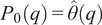 . Taking this pricing rule as given, upon learning that
$ A=1 $
. Taking this pricing rule as given, upon learning that
$ A=1 $
 , the speculator’s expected profit from purchasing
$ x $
, the speculator’s expected profit from purchasing
$ x $
 shares is strictly positive:
$ \frac{x}{2}\left(1-\theta \right)>0 $
shares is strictly positive:
$ \frac{x}{2}\left(1-\theta \right)>0 $
 . His expected trading profit from purchasing
$ x $
. His expected trading profit from purchasing
$ x $
 shares upon learning that
$ A=0 $
shares upon learning that
$ A=0 $
 is strictly negative:
$ -\frac{x}{2}\left(1+\theta \right)<0 $
is strictly negative:
$ -\frac{x}{2}\left(1+\theta \right)<0 $
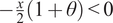 . Similarly, his expected profit from purchasing
$ x $
. Similarly, his expected profit from purchasing
$ x $
 shares upon learning nothing is also strictly negative:
$ \frac{x}{2}\left(\theta -1\right)<0 $
shares upon learning nothing is also strictly negative:
$ \frac{x}{2}\left(\theta -1\right)<0 $
 . Hence, the speculator buys
$ x $
. Hence, the speculator buys
$ x $
 shares if and only if he learns that
$ A=1 $
shares if and only if he learns that
$ A=1 $
 .
.
Proof of Lemma 2. Suppose the manager buys back
$ x $
 shares with probabilities
$ {b}_1 $
shares with probabilities
$ {b}_1 $
 and
$ {b}_0 $
and
$ {b}_0 $
 when
$ A=1 $
when
$ A=1 $
 and
$ A=0 $
and
$ A=0 $
 , respectively, where
$ {b}_1\ge {b}_0 $
, respectively, where
$ {b}_1\ge {b}_0 $
 . Additionally, suppose the speculator buys
$ x $
. Additionally, suppose the speculator buys
$ x $
 shares if and only if he learns that firm fundamentals are high. Noise traders submit an order of
$ -x $
shares if and only if he learns that firm fundamentals are high. Noise traders submit an order of
$ -x $
 and
$ 0 $
and
$ 0 $
 with equal probability. The possible order flows in the different states of the world are as follows:

Table A2 Long description
The table has six rows and eight columns. The columns are State, Firm q sub B, Speculator q sub S, Probability, and four Order Flow columns. The first row under headers is for A equals 0, firm 0, speculator 0, probability open parenthesis 1 minus theta close parenthesis open parenthesis 1 minus b sub 0 close parenthesis, order flow minus x, 0, blank, blank. Second row: A equals 0, firm x, speculator 0, probability open parenthesis 1 minus theta close parenthesis b sub 0, order flow blank, 0, x, blank. Third row: A equals 1, firm 0, speculator 0, probability theta open parenthesis 1 minus phi close parenthesis open parenthesis 1 minus b sub 1 close parenthesis, order flow minus x, 0, blank, blank. Fourth row: A equals 1, firm x, speculator 0, probability theta open parenthesis 1 minus phi close parenthesis b sub 1, order flow blank, 0, x, blank. Fifth row: A equals 1, firm 0, speculator x, probability theta phi open parenthesis 1 minus b sub 1 close parenthesis, order flow blank, 0, x, blank. Sixth row: A equals 1, firm x, speculator x, probability theta phi b sub 1, order flow blank, blank, x, 2 x.
and imply that the market’s posterior belief is

An order flow of
$ q=2x $
 fully reveals that
$ A=1 $
fully reveals that
$ A=1 $
 ; hence,
$ {P}_B(2x)=1 $
; hence,
$ {P}_B(2x)=1 $
 . An order flow of
$ q=-x $
. An order flow of
$ q=-x $
 fully reveals that no buybacks occurred; hence,
$ {P}_B\left(-x\right)={\hat{\theta}}_B\left(-x\right) $
fully reveals that no buybacks occurred; hence,
$ {P}_B\left(-x\right)={\hat{\theta}}_B\left(-x\right) $
 . When the order flow is
$ 0 $
. When the order flow is
$ 0 $
 , the market makers’ pricing rule satisfies

implying that

Similarly, when the order flow is
$ x $
 , the market makers’ pricing rule satisfies

implying that

Therefore, the equilibrium pricing rule is

Substituting in
$ {b}_1=1 $
 yields the pricing rule in the lemma. Given this pricing rule, upon learning that
$ A=1 $
yields the pricing rule in the lemma. Given this pricing rule, upon learning that
$ A=1 $
 , the speculator’s expected profit from purchasing
$ x $
, the speculator’s expected profit from purchasing
$ x $
 shares is positive. His expected trading profit from purchasing
$ x $
shares is positive. His expected trading profit from purchasing
$ x $
 shares upon learning that
$ A=0 $
shares upon learning that
$ A=0 $
 or learning nothing is strictly negative. Hence, the speculator buys
$ x $
or learning nothing is strictly negative. Hence, the speculator buys
$ x $
 shares if and only if he learns that
$ A=1 $
shares if and only if he learns that
$ A=1 $
 . Note that the effects of buyback profits and losses show up in the pricing rule via the scale of the buyback program
$ k $
. Note that the effects of buyback profits and losses show up in the pricing rule via the scale of the buyback program
$ k $
 .
.
Proof of Lemma 3. Recall that

and

Hence,
$ \Delta {\hat{\theta}}_B>\Delta {\hat{\theta}}_0\iff {b}_0<1 $
 . Taking its derivative with respect to
$ {b}_0 $
. Taking its derivative with respect to
$ {b}_0 $
 yields

Proof of Lemma 4. Recall that

where

is the magnitude of expected trading gains and

is the magnitude of expected trading losses. Hence,
$ \Delta {V}_B>\Delta {V}_0 $
 . Note that


and

Hence,
$ \frac{\mathrm{\partial \Delta }{V}_B}{\partial {b}_0}>0 $
 (i.e., less informative buybacks magnify the increase in per-share value dispersion).
Proof of Lemma 5. Recall that

Taking the derivative of
$ \Delta {P}_B $
 with respect to
$ {b}_0 $
with respect to
$ {b}_0 $
 yields

if and only if

Note that the right-hand side of the inequality (
$ RHS $
 ) strictly decreases with
$ {b}_0 $
) strictly decreases with
$ {b}_0 $
 :
:

because
$ \theta \phi \left(1+k\right)<1 $
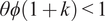 . As a result, it achieves its minimum when
$ {b}_0=1 $
. As a result, it achieves its minimum when
$ {b}_0=1 $
 . Note that

because
$ \phi k\left(1+k\right)<{\left(1+k\right)}^2 $
 and
$ \left(1-\theta \right)\left(1-\phi \right)<\left(1-\theta \phi \right)\left(1-\theta \phi \right) $
and
$ \left(1-\theta \right)\left(1-\phi \right)<\left(1-\theta \phi \right)\left(1-\theta \phi \right) $
 . Hence,
$ \frac{\mathrm{\partial \Delta }{P}_B}{\partial {b}_0}<0 $
. Hence,
$ \frac{\mathrm{\partial \Delta }{P}_B}{\partial {b}_0}<0 $
 .
.
Proof of Proposition 1. The speculator’s expected trading profit can be written as

Taking the derivative of
$ {\Pi}_B $
 with respect to
$ {b}_0 $
with respect to
$ {b}_0 $
 yields

In the benchmark without buybacks, the speculator’s expected trading profit is
$ {\Pi}_0=\phi x\theta \left(1-\theta \right)\frac{1}{2} $
 . Hence,

noting that
$ \frac{\partial {\overline{b}}_0}{\partial k}<0 $
 and
$ \frac{\partial {\overline{b}}_0}{\partial \theta }>0 $
and
$ \frac{\partial {\overline{b}}_0}{\partial \theta }>0 $
 .
.
Proof of Lemma 6. The expected per-share trading gain from the firm’s buyback activities is

strictly so when
$ {b}_0<1 $
 and
$ \phi <1 $
and
$ \phi <1 $
 . Taking its derivative with respect to
$ {b}_0 $
. Taking its derivative with respect to
$ {b}_0 $
 yields

Proof of Proposition 2. Recall that

Taking its derivative with respect to b 0 yields

The first (positive) term inside the brackets is bounded below for all
$ {b}_0\in \left[0,1\right] $
 and
$ \phi >0 $
and
$ \phi >0 $
 :
:

The magnitude of the second (negative) term is bounded above for all
$ {b}_0\in \left[0,1\right] $
 and
$ \phi >0 $
and
$ \phi >0 $
 :
$ \frac{\phi x\theta}{{\left[\theta +\left(1-\theta \right){b}_0\right]}^2}\le \frac{\phi x}{\theta } $
:
$ \frac{\phi x\theta}{{\left[\theta +\left(1-\theta \right){b}_0\right]}^2}\le \frac{\phi x}{\theta } $
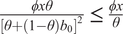 . Moreover,

for all
$ {b}_0\in \left[0,1\right] $
 . Hence,
$ \frac{\partial {U}_B^E}{\partial {b}_0}>0 $
. Hence,
$ \frac{\partial {U}_B^E}{\partial {b}_0}>0 $
 for
$ \phi $
for
$ \phi $
 sufficiently low. For example, one sufficient upper bound on
$ \phi $
sufficiently low. For example, one sufficient upper bound on
$ \phi $
 would be

The last inequality is satisfied if
$ \phi <\frac{H_2}{H_2+\frac{x}{\theta }}:= \underline{\phi} $
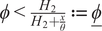 , where
$ \underline{\phi}\in \left(0,1\right) $
, where
$ \underline{\phi}\in \left(0,1\right) $
 .
.
Proof of Proposition 3. Recall that

Taking its derivative with respect to b 0 yields

As
$ \phi \to 1 $
 , the first term inside the brackets vanishes, leaving

for all
$ {b}_0\in \left[0,1\right] $
 . Hence, by continuity, for
$ \phi $
. Hence, by continuity, for
$ \phi $
 sufficiently large,
$ \frac{\partial {U}_B^E}{\partial {b}_0}<0 $
sufficiently large,
$ \frac{\partial {U}_B^E}{\partial {b}_0}<0 $
 , implying that the payoff of liquidity-exposed shareholders increases with buyback informativeness.
Proof of Corollary 1. When
$ {b}_0=1 $
 , Lemma 6 implies
$ \unicode{x1D53C}\left[T\right]=0 $
, Lemma 6 implies
$ \unicode{x1D53C}\left[T\right]=0 $
 . Moreover, Proposition 1 implies that
$ {\Pi}_B>{\Pi}_0 $
. Moreover, Proposition 1 implies that
$ {\Pi}_B>{\Pi}_0 $
 . Hence,
$ {\left.{U}_B^E\right|}_{b_0=1}-{U}_0^E<0 $
. Hence,
$ {\left.{U}_B^E\right|}_{b_0=1}-{U}_0^E<0 $
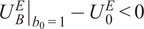 when
$ \phi >0 $
when
$ \phi >0 $
 .
.
Proof of Proposition 4. Suppose the manager executes buybacks—buying back
$ x $
 shares—with probabilities
$ {b}_1 $
shares—with probabilities
$ {b}_1 $
 and
$ {b}_0 $
and
$ {b}_0 $
 upon learning that
$ A=1 $
upon learning that
$ A=1 $
 and
$ A=0 $
and
$ A=0 $
 , respectively. Moreover, the speculator buys
$ x $
, respectively. Moreover, the speculator buys
$ x $
 shares if and only if he learns that
$ A=1 $
shares if and only if he learns that
$ A=1 $
 . The proof of Lemma 2 shows that the market’s pricing rule is given by

Note that for any (
$ {b}_1,{b}_0 $
 ), the equilibrium pricing rule is increasing because of the speculator’s informed trading. The manager executes buybacks to maximize
$ \unicode{x1D53C}\left[\omega {P}_B+V\right] $
), the equilibrium pricing rule is increasing because of the speculator’s informed trading. The manager executes buybacks to maximize
$ \unicode{x1D53C}\left[\omega {P}_B+V\right] $
 . As a result, when the manager learns that
$ A=1 $
. As a result, when the manager learns that
$ A=1 $
 , she strictly prefers to execute buybacks (
$ {q}_B=x $
, she strictly prefers to execute buybacks (
$ {q}_B=x $
 ). Doing so increases the expected market-clearing price at
$ t=1 $
). Doing so increases the expected market-clearing price at
$ t=1 $
 (due to
$ {P}_B(q) $
(due to
$ {P}_B(q) $
 increasing in
$ q $
increasing in
$ q $
 ) and the per-share value at
$ t=2 $
) and the per-share value at
$ t=2 $
 (due to trading profits). Hence,
$ {b}_1^{\ast }=1 $
(due to trading profits). Hence,
$ {b}_1^{\ast }=1 $
 , simplifying the pricing rule:

Suppose
$ {b}_0^{\ast }=0 $
 . When the manager learns that
$ A=0 $
. When the manager learns that
$ A=0 $
 , she strictly prefers not to execute buybacks if and only if

which corresponds to

Similarly, suppose
$ {b}_0^{\ast }=1 $
 . When the manager learns that
$ A=0 $
. When the manager learns that
$ A=0 $
 , she strictly prefers to execute buybacks if and only if

Note that
$ \underline{\omega}=k\left(1+\frac{\theta \left(1-\phi \right)\left(1+k\right)}{\theta \left(1-\phi \right)\left(1+k\right)+\left(1-\theta \right)}\right)<k\left(1+\frac{\left(1-\phi \right)}{\theta \left(1-\phi \right)+\left(1-\theta \right)}\right)=\overline{\omega} $
 if and only if

Hence,
$ 1>\theta \phi \left(1+k\right) $
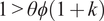 ensures that
$ \underline{\omega}<\overline{\omega} $
ensures that
$ \underline{\omega}<\overline{\omega} $
 , and that the manager’s execution strategy is unique. Otherwise, we have
$ \overline{\omega}\le \underline{\omega} $
, and that the manager’s execution strategy is unique. Otherwise, we have
$ \overline{\omega}\le \underline{\omega} $
 , and there are multiple equilibria (
$ {b}_0^{\ast }=0 $
, and there are multiple equilibria (
$ {b}_0^{\ast }=0 $
 and
$ {b}_0^{\ast }=1 $
and
$ {b}_0^{\ast }=1 $
 ) when
$ \omega \in \left[\overline{\omega},\underline{\omega}\right] $
) when
$ \omega \in \left[\overline{\omega},\underline{\omega}\right] $
 .
.
Finally, suppose
$ {b}_0^{\ast}\in \left(0,1\right) $
 . When the manager learns that
$ A=0 $
. When the manager learns that
$ A=0 $
 , she is indifferent between executing buybacks and not executing buybacks if and only if
$ \left(\omega -k\right){P}_B(x)={kP}_B(0) $
, she is indifferent between executing buybacks and not executing buybacks if and only if
$ \left(\omega -k\right){P}_B(x)={kP}_B(0) $
 , which corresponds to

Note that
$ {b}_0^{\ast }=0 $
 when
$ \omega =\underline{\omega} $
when
$ \omega =\underline{\omega} $
 , and
$ {b}_0^{\ast }=1 $
, and
$ {b}_0^{\ast }=1 $
 when
$ \omega =\overline{\omega} $
when
$ \omega =\overline{\omega} $
 . Moreover,
$ {b}_0^{\ast } $
. Moreover,
$ {b}_0^{\ast } $
 strictly increases with
$ \omega $
strictly increases with
$ \omega $
 on
$ \left[\underline{\omega},\overline{\omega}\right] $
on
$ \left[\underline{\omega},\overline{\omega}\right] $
 :
:

Proof of Proposition 5. Recall from the proof of Proposition 4 that

and

for
$ \omega \in \left[\underline{\omega},\overline{\omega}\right] $
 . Note that
$ \omega \in \left[\underline{\omega},\overline{\omega}\right] $
. Note that
$ \omega \in \left[\underline{\omega},\overline{\omega}\right] $
 implies that
$ \omega >k $
implies that
$ \omega >k $
 and
$ \omega <2k $
and
$ \omega <2k $
 .
.
Taking the derivative of
$ \underline{\omega} $
 with respect to
$ \theta $
with respect to
$ \theta $
 yields

Similarly, taking the derivative of
$ \overline{\omega} $
 with respect to
$ \theta $
with respect to
$ \theta $
 yields

Moreover, the expression for
$ {b}_0^{\ast } $
 can be rearranged as

which decreases in
$ \theta $
 . Hence, for any fixed
$ \omega $
. Hence, for any fixed
$ \omega $
 , higher
$ \theta $
, higher
$ \theta $
 implies lower
$ {b}_0^{\ast } $
implies lower
$ {b}_0^{\ast } $
 (i.e., higher buyback informativeness).
Taking the derivative of
$ \underline{\omega} $
 with respect to
$ k $
with respect to
$ k $
 yields

Taking the derivative of
$ \overline{\omega} $
 with respect to
$ k $
with respect to
$ k $
 yields

Moreover, the expression for
$ {b}_0^{\ast } $
 can be rearranged as

which decreases in
$ k $
 , which enters negatively in the numerator and positively in the denominator. Hence, for any fixed
$ \omega $
, which enters negatively in the numerator and positively in the denominator. Hence, for any fixed
$ \omega $
 , higher
$ k $
, higher
$ k $
 implies lower
$ {b}_0^{\ast } $
implies lower
$ {b}_0^{\ast } $
 (i.e., higher buyback informativeness).
Taking the derivative of
$ \underline{\omega} $
 with respect to
$ \phi $
with respect to
$ \phi $
 yields

Taking the derivative of
$ \overline{\omega} $
 with respect to
$ \phi $
with respect to
$ \phi $
 yields

Moreover, the expression for
$ {b}_0^{\ast } $
 can be rearranged as

which increases in
$ \phi $
 because
$ \phi $
because
$ \phi $
 enters positively in the numerator and negatively in the denominator. Hence, for any fixed
$ \omega $
enters positively in the numerator and negatively in the denominator. Hence, for any fixed
$ \omega $
 , higher
$ \phi $
, higher
$ \phi $
 implies higher
$ {b}_0^{\ast } $
implies higher
$ {b}_0^{\ast } $
 (i.e., lower buyback informativeness).
Appendix B. Proofs: Extensions
Proof of Lemma 7. Recall that

Hence, the expected per-share profit generated by the buyback program is

noting that
$ {\theta}_x=\frac{\theta }{\theta +\left(1-\theta \right){b}_0}\iff {\theta}_x\left(1-\theta \right){b}_0=\theta \left(1-{\theta}_x\right) $
 .
.
Proof of Proposition 6. Given the pricing rule
$ {P}_B^D $
 , the expected trading profit of the speculator is

which strictly increases with
$ {b}_0 $
 :
:

Moreover,
$ {\left.{\Pi}_B^D\right|}_{b=0}<{\Pi}_0 $
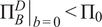 and
$ {\left.{\Pi}_B^D\right|}_{b_0=1}>{\Pi}_0 $
and
$ {\left.{\Pi}_B^D\right|}_{b_0=1}>{\Pi}_0 $
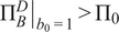 , implying that there exists a threshold
$ {\overline{b}}_0^D $
, implying that there exists a threshold
$ {\overline{b}}_0^D $
 such that
$ {\Pi}_B^D<{\Pi}_0\iff {b}_0<{\overline{b}}_0^D $
such that
$ {\Pi}_B^D<{\Pi}_0\iff {b}_0<{\overline{b}}_0^D $
 .
.
Proof of Proposition 7. This proof closely follows the logic of the proof of Proposition 4. First, executing buybacks when
$ A=1 $
 increases the expected market-clearing price at
$ t=1 $
increases the expected market-clearing price at
$ t=1 $
 , strictly so if
$ {b}_0<1 $
, strictly so if
$ {b}_0<1 $
 . Moreover, these buybacks also generate positive trading profits if
$ {b}_0>0 $
. Moreover, these buybacks also generate positive trading profits if
$ {b}_0>0 $
 . Hence, executing buybacks upon learning that
$ A=1 $
. Hence, executing buybacks upon learning that
$ A=1 $
 is strictly dominant:
$ {b}_1^{\ast }=1 $
is strictly dominant:
$ {b}_1^{\ast }=1 $
 .
.
Second, the manager faces a trade-off upon observing
$ A=0 $
 . If she does not execute, the lack of pre-trade disclosure fully reveals that
$ A=0 $
. If she does not execute, the lack of pre-trade disclosure fully reveals that
$ A=0 $
 , implying that the market-clearing stock price at
$ t=1 $
, implying that the market-clearing stock price at
$ t=1 $
 and the per-share value at
$ t=2 $
and the per-share value at
$ t=2 $
 are zero. If she does execute, the expected market-clearing price is
$ \frac{1}{2}\left({P}_B^D(0)+{P}_B^D(x)\right)>0 $
are zero. If she does execute, the expected market-clearing price is
$ \frac{1}{2}\left({P}_B^D(0)+{P}_B^D(x)\right)>0 $
 . In this case, she prefers not to execute buybacks if and only if

She strictly prefers to execute buybacks if and only if

Recall that in the baseline model, the threshold
$ \underline{\omega} $
 is
is

Hence, for all
$ \omega $
 , the manager is more likely to buy back shares in the low-fundamental state in the pretrade disclosure regime than in the baseline without disclosure.
Proof of Lemma 8. Recall that the market’s posterior beliefs are

and

Taking the derivative of
$ {\hat{\theta}}_B\left(-x\right) $
 ,
$ {\hat{\theta}}_B(0) $
,
$ {\hat{\theta}}_B(0) $
 , and
$ {\hat{\theta}}_B(x) $
, and
$ {\hat{\theta}}_B(x) $
 with respect to
$ {b}_1 $
with respect to
$ {b}_1 $
 yields


and

Hence,

Taking the derivative of
$ {\hat{\theta}}_B\left(-x\right) $
 ,
$ {\hat{\theta}}_B(0) $
,
$ {\hat{\theta}}_B(0) $
 , and
$ {\hat{\theta}}_B(x) $
, and
$ {\hat{\theta}}_B(x) $
 with respect to
$ {b}_0 $
with respect to
$ {b}_0 $
 yields


and

Hence,

Recall that
$ \Delta {\hat{\theta}}_0=\frac{1}{2}\phi \frac{\left(1-\theta \right)}{\theta \left(1-\phi \right)+\left(1-\theta \right)} $
 . Fix
$ {b}_0<1 $
. Fix
$ {b}_0<1 $
 and note that

and

Hence, the monotonicity of
$ \Delta {\hat{\theta}}_B $
 with respect to
$ {b}_1 $
with respect to
$ {b}_1 $
 implies that there exists some
$ {\underline{b}}_1\left({b}_0\right)\in \left({b}_0,1\right) $
implies that there exists some
$ {\underline{b}}_1\left({b}_0\right)\in \left({b}_0,1\right) $
 such that
$ \Delta {\hat{\theta}}_B>\Delta {\hat{\theta}}_0\iff {b}_1>{\underline{b}}_1\left({b}_0\right) $
such that
$ \Delta {\hat{\theta}}_B>\Delta {\hat{\theta}}_0\iff {b}_1>{\underline{b}}_1\left({b}_0\right) $
 . For completeness, note that
$ {b}_1={b}_0=1 $
. For completeness, note that
$ {b}_1={b}_0=1 $
 implies that
$ \Delta {\hat{\theta}}_B=\Delta {\hat{\theta}}_0 $
implies that
$ \Delta {\hat{\theta}}_B=\Delta {\hat{\theta}}_0 $
 , implying that
$ {\underline{b}}_1(1)=1 $
, implying that
$ {\underline{b}}_1(1)=1 $
 .
.
Fix
$ {b}_1>0 $
 . Note that

and
$ {\left.\Delta {\hat{\theta}}_B\right|}_{b_0={b}_1=b}<\Delta {\hat{\theta}}_0 $
 . Hence, the monotonicity of
$ \Delta {\hat{\theta}}_B $
. Hence, the monotonicity of
$ \Delta {\hat{\theta}}_B $
 with respect to
$ {b}_0 $
with respect to
$ {b}_0 $
 implies that there exists some
$ {\underline{b}}_0\left({b}_1\right)\in \left(0,{b}_1\right) $
implies that there exists some
$ {\underline{b}}_0\left({b}_1\right)\in \left(0,{b}_1\right) $
 such that
$ \Delta {\hat{\theta}}_B>\Delta {\hat{\theta}}_0\iff {b}_0<{\underline{b}}_0\left({b}_1\right) $
such that
$ \Delta {\hat{\theta}}_B>\Delta {\hat{\theta}}_0\iff {b}_0<{\underline{b}}_0\left({b}_1\right) $
 .
.
Proof of Lemma 9. Recall that

where

and

Taking the derivative of
$ {\overline{T}}_G $
 and
$ {\overline{T}}_L $
and
$ {\overline{T}}_L $
 with respect to
$ {b}_0 $
with respect to
$ {b}_0 $
 yields

and

Note that
$ {\overline{T}}_L+{b}_0\frac{\partial {\overline{T}}_L}{\partial {b}_0} $
 simplifies to

Hence,

Taking the derivative of
$ {\overline{T}}_G $
 with respect to
$ {b}_1 $
with respect to
$ {b}_1 $
 yields

Note that
$ {\overline{T}}_G+{b}_1\frac{\partial {\overline{T}}_G}{\partial {b}_1} $
 simplifies to

Taking the derivative of
$ {\overline{T}}_L $
 with respect to
$ {b}_1 $
with respect to
$ {b}_1 $
 yields

which is bounded for all
$ {b}_0\in \left[0,1\right] $
 . Hence,
$ {\left.\frac{\mathrm{\partial \Delta }{V}_B}{\partial {b}_1}\right|}_{b_0=0}>0 $
. Hence,
$ {\left.\frac{\mathrm{\partial \Delta }{V}_B}{\partial {b}_1}\right|}_{b_0=0}>0 $
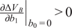 , implying that value dispersion increases with
$ {b}_1 $
, implying that value dispersion increases with
$ {b}_1 $
 when
$ {b}_0 $
when
$ {b}_0 $
 is sufficiently small.
Proof of Proposition 8. Recall from the proof of Lemma 2 that when the manager follows the buyback strategy (
$ {b}_1,{b}_0 $
 ) and the speculator buys if and only if he observes
$ A=1 $
) and the speculator buys if and only if he observes
$ A=1 $
 , the distribution of the order flow is as follows:

Table B1 Long description
The header row lists State, Firm q sub B, Speculator q sub S, Probability, and four Order Flow columns. The first row, with State A equals 0, Firm 0, Speculator 0, Probability open parenthesis 1 minus theta close parenthesis open parenthesis 1 minus b sub 0 close parenthesis, Order Flow minus x, 0, blank, blank. Second row, State A equals 0, Firm x, Speculator 0, Probability open parenthesis 1 minus theta close parenthesis b sub 0, Order Flow blank, 0, x, blank. Third row, State A equals 1, Firm 0, Speculator 0, Probability theta open parenthesis 1 minus phi close parenthesis open parenthesis 1 minus b sub 1 close parenthesis, Order Flow minus x, 0, blank, blank. Fourth row, State A equals 1, Firm x, Speculator 0, Probability theta open parenthesis 1 minus phi close parenthesis b sub 1, Order Flow blank, 0, x, blank. Fifth row, State A equals 1, Firm 0, Speculator x, Probability theta phi open parenthesis 1 minus b sub 1 close parenthesis, Order Flow blank, 0, x, blank. Sixth row, State A equals 1, Firm x, Speculator x, Probability theta phi b sub 1, Order Flow blank, blank, x, 2 x.
and the equilibrium pricing rule is

The speculator’s expected trading profit is

For algebraic convenience, let us split
$ {\Pi}_B $
 into its two addends:
$ {\Pi}_B={\Pi}_{B1}+{\Pi}_{B2} $
into its two addends:
$ {\Pi}_B={\Pi}_{B1}+{\Pi}_{B2} $
 , where

and

Note that

and

implying that
$ \frac{\partial {\Pi}_B}{\partial {b}_0}>0 $
 . Note that

and is bounded above by

Moreover,

which is bounded above by

Hence,

and note that

which is negative whenever

Note that
$ \sqrt{k}<1 $
 because
$ k<1 $
because
$ k<1 $
 and
and

whenever
$ {b}_1\ge {b}_0 $
 . Hence, we have
$ \frac{\partial {\Pi}_B}{\partial {b}_1}<0 $
. Hence, we have
$ \frac{\partial {\Pi}_B}{\partial {b}_1}<0 $
 whenever
$ k<1 $
whenever
$ k<1 $
 and
$ {b}_1\ge {b}_0 $
and
$ {b}_1\ge {b}_0 $
 .
.
When buybacks are uninformed (
$ {b}_1={b}_0=b $
 ), the speculator’s expected trading profit is

In this case,

In addition, note that for a fixed
$ {b}_1>0 $
 ,
,

and for a fixed
$ {b}_0<{\overline{b}}_0 $
 , with
$ {\overline{b}}_0 $
, with
$ {\overline{b}}_0 $
 defined in Proposition 1,
$ {\left.{\Pi}_B\right|}_{b_1=1}<{\Pi}_0 $
defined in Proposition 1,
$ {\left.{\Pi}_B\right|}_{b_1=1}<{\Pi}_0 $
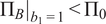 . The monotonicity of
$ {\Pi}_B $
. The monotonicity of
$ {\Pi}_B $
 with respect to
$ {b}_0 $
with respect to
$ {b}_0 $
 and
$ {b}_1 $
and
$ {b}_1 $
 (when
$ k<1 $
(when
$ k<1 $
 ) establishes the claim of the proposition.
Appendix C. Additional Results and Robustness
C.A Other Trading Outcomes
The competition and dispersion effects of a stock buyback program also affect the distribution of the firm’s stock return from
$ t=1 $
 to
$ t=2 $
to
$ t=2 $
 . In the benchmark without buybacks, the firm’s stock return from
$ t=1 $
. In the benchmark without buybacks, the firm’s stock return from
$ t=1 $
 to
$ t=2 $
to
$ t=2 $
 is
$ {r}_0=\frac{A-{P}_0}{P_0} $
is
$ {r}_0=\frac{A-{P}_0}{P_0} $
 , where
$ {P}_0 $
, where
$ {P}_0 $
 is the firm’s market-clearing price at
$ t=1 $
is the firm’s market-clearing price at
$ t=1 $
 described by Lemma 1. With buybacks, the firm’s stock return becomes
$ {r}_B=\frac{V-{P}_B}{P_B} $
described by Lemma 1. With buybacks, the firm’s stock return becomes
$ {r}_B=\frac{V-{P}_B}{P_B} $
 , where
$ {P}_B $
, where
$ {P}_B $
 is the firm’s market-clearing stock price at
$ t=1 $
is the firm’s market-clearing stock price at
$ t=1 $
 described by Lemma 2 and
$ V $
described by Lemma 2 and
$ V $
 is the firm’s per-share value at
$ t=2 $
is the firm’s per-share value at
$ t=2 $
 .
.
C.A.1 Return Volatility
If the execution of the buyback program is informed (
$ {b}_0<1 $
 ), then the competition effect increases the informativeness of the order flow. As a result, the firm’s market-clearing price at
$ t=1 $
), then the competition effect increases the informativeness of the order flow. As a result, the firm’s market-clearing price at
$ t=1 $
 is more likely to reflect its fundamentals. Hence, the competition effect of informed buybacks tends to push the distribution of the firm’s stock return toward its expected value, decreasing the volatility of returns.
The dispersion effect works in the opposite direction through buyback trading gains and losses. When the firm’s fundamentals are high, buybacks generate trading profits that increase the firm’s
$ t=2 $
 per-share value and the realized stock return. When the firm’s fundamentals are low, buybacks generate trading losses that decrease the firm’s
$ t=2 $
per-share value and the realized stock return. When the firm’s fundamentals are low, buybacks generate trading losses that decrease the firm’s
$ t=2 $
 per-share value and the realized stock return. Thus, the dispersion effect of buybacks tends to shift the distribution of the firm’s stock return away from its expected value, increasing the volatility of returns.
The overall impact of a buyback program on the volatility of the firm’s stock return depends on the relative magnitude of these effects. The first effect dominates when the execution of the buyback program is sufficiently informed. Otherwise, the second effect dominates:
Proposition C.1. A stock buyback program decreases the volatility of the firm’s stock return from
$ t=1 $
 to
$ t=2 $
to
$ t=2 $
 if and only if its execution is sufficiently informed:
$ \exists {\overline{b}}_0^r\in \left(0,1\right) $
if and only if its execution is sufficiently informed:
$ \exists {\overline{b}}_0^r\in \left(0,1\right) $
 such that
$ Var\left({r}_B\right)< Var\left({r}_0\right)\iff {b}_0<{\overline{b}}_0^r $
such that
$ Var\left({r}_B\right)< Var\left({r}_0\right)\iff {b}_0<{\overline{b}}_0^r $
 .
.
Proof of Proposition C.1. Because the market is risk-neutral and does not discount for time, the break-even condition implies that the market-clearing price at
$ t=1 $
 is set so that the expected stock return from
$ t=1 $
is set so that the expected stock return from
$ t=1 $
 to
$ t=2 $
to
$ t=2 $
 is
$ 0 $
is
$ 0 $
 . In the benchmark without a stock buyback program, Lemma 1 implies that the volatility of the firm’s stock return is

Recall from Lemma 2 that the equilibrium order flow with buybacks is

Table C1 Long description
The header row lists columns: State, Firm q sub B, Speculator q sub S, Probability, and Order Flow (spanning four columns). The first row has State A equals 0, Firm 0, Speculator 0, Probability open parenthesis 1 minus theta close parenthesis open parenthesis 1 minus b sub 0 close parenthesis, Order Flow negative x, 0, blank, blank. The second row has State A equals 0, Firm x, Speculator 0, Probability open parenthesis 1 minus theta close parenthesis b sub 0, Order Flow blank, 0, x, blank. The third row has State A equals 1, Firm x, Speculator 0, Probability theta open parenthesis 1 minus phi close parenthesis, Order Flow blank, 0, x, blank. The fourth row has State A equals 1, Firm x, Speculator x, Probability theta phi, Order Flow blank, blank, x, 2 x.
Moreover, the order flow is fully revealing when
$ q=-x $
 and
$ q=2x $
and
$ q=2x $
 , implying that the realized return in those states is
$ 0 $
, implying that the realized return in those states is
$ 0 $
 . Hence, the volatility of the firm’s stock return is

Note that
$ \frac{dVar\left({r}_B\right)}{db_0}>0 $
 and
and

and

Hence, the monotonicity of
$ Var\left({r}_B\right) $
 with respect to
$ {b}_0 $
with respect to
$ {b}_0 $
 implies that there exists a
$ {\overline{b}}_0^r\in \left(0,1\right) $
implies that there exists a
$ {\overline{b}}_0^r\in \left(0,1\right) $
 such that
$ Var\left({r}_B\right)< Var\left({r}_0\right)\iff {b}_0<{\overline{b}}_0^r $
such that
$ Var\left({r}_B\right)< Var\left({r}_0\right)\iff {b}_0<{\overline{b}}_0^r $
 .
.
C.A.2 Return Following Buybacks
The informativeness of buybacks also influences the firm’s expected stock return from
$ t=1 $
 to
$ t=2 $
to
$ t=2 $
 following buybacks. When buybacks are more informed, a buyback is more likely to occur when fundamentals are high. Conditional on a buyback occurring, then, higher informativeness implies that fundamentals are more likely to be high—leading to higher prices at
$ t=2 $
following buybacks. When buybacks are more informed, a buyback is more likely to occur when fundamentals are high. Conditional on a buyback occurring, then, higher informativeness implies that fundamentals are more likely to be high—leading to higher prices at
$ t=2 $
 once fundamentals become public. In addition, more informed buybacks are more likely to earn trading profits, which further increase the firm’s per-share value at
$ t=2 $
once fundamentals become public. In addition, more informed buybacks are more likely to earn trading profits, which further increase the firm’s per-share value at
$ t=2 $
 . More informative buybacks also increase the firm’s stock price at
$ t=1 $
. More informative buybacks also increase the firm’s stock price at
$ t=1 $
 . However, because the order flow at
$ t=1 $
. However, because the order flow at
$ t=1 $
 is not fully revealing, the firm’s per-share value at
$ t=2 $
is not fully revealing, the firm’s per-share value at
$ t=2 $
 following buybacks increases relative to its stock price at
$ t=1 $
following buybacks increases relative to its stock price at
$ t=1 $
 .
.
Proposition C.2. If the execution of the stock buyback program is informed (
$ {b}_0<1 $
 ), then the expected return of the firm’s stock from
$ t=1 $
), then the expected return of the firm’s stock from
$ t=1 $
 to
$ t=2 $
to
$ t=2 $
 following buybacks is positive and decreases in
$ {b}_0 $
following buybacks is positive and decreases in
$ {b}_0 $
 .
.
Proposition C.2 predicts a positive association between the informativeness of buybacks and subsequent returns, consistent with the empirical findings of Bonaime and Ryngaert (Reference Bonaime and Ryngaert2013), who document higher stock returns following buybacks when the firm’s insiders and the buyback program trade in the same direction.
Proof of Proposition C.2. Lemma 2 implies that the firm’s conditional expected return following buybacks is

when buybacks are informed (
$ {b}_0<1 $
 ), noting that the realized return when the order flow is fully revealing (i.e.,
$ q=-x $
), noting that the realized return when the order flow is fully revealing (i.e.,
$ q=-x $
 ,
$ q=2x $
,
$ q=2x $
 ) is
$ 0 $
) is
$ 0 $
 . Taking the derivative of
$ E\left[{r}_B|{q}_B=x\right] $
. Taking the derivative of
$ E\left[{r}_B|{q}_B=x\right] $
 with respect to
$ {b}_0 $
with respect to
$ {b}_0 $
 yields

C.B Short Selling
For simplicity, the baseline model assumes that the speculator cannot sell short. This analysis relaxes this assumption, allowing the speculator to submit an order
$ {q}_S\in \left\{-x,0,x\right\} $
 , and demonstrates that the framework’s main conclusion—that uninformed buybacks hurt shareholders—extends to this setting.Footnote
27
, and demonstrates that the framework’s main conclusion—that uninformed buybacks hurt shareholders—extends to this setting.Footnote
27
The following lemma characterizes the benchmark trading equilibrium featuring short selling:
Lemma C.1. In the absence of a buyback program, the equilibrium pricing rule is

and the speculator buys
$ x $
 shares if he learns that firm fundamentals are high (
$ A=1 $
shares if he learns that firm fundamentals are high (
$ A=1 $
 ), short sells
$ x $
), short sells
$ x $
 shares if he learns that firm fundamentals are low (
$ A=0 $
shares if he learns that firm fundamentals are low (
$ A=0 $
 ), and abstains otherwise.
Proof of Lemma C.1. The logic of this proof closely follows that of Lemma 1. Suppose the speculator buys
$ x $
 shares if he learns that firm fundamentals are high (
$ A=1 $
shares if he learns that firm fundamentals are high (
$ A=1 $
 ), short sells
$ x $
), short sells
$ x $
 shares if he learns that firm fundamentals are low (
$ A=0 $
shares if he learns that firm fundamentals are low (
$ A=0 $
 ), and abstains otherwise. In this case, the market expects the following distribution of order flow:

Table C2 Long description
The table has four rows, each representing a state defined by A equals 0 or 1. For A equals 0, the first row lists speculator as minus x, probability as open parenthesis 1 minus theta close parenthesis phi, order flow as minus 2 x, minus x, and two empty cells. The second row for A equals 0 has speculator 0, probability open parenthesis 1 minus theta close parenthesis open parenthesis 1 minus phi close parenthesis, order flow with two empty cells, minus x, 0, and one empty cell. For A equals 1, the third row lists speculator 0, probability theta open parenthesis 1 minus phi close parenthesis, order flow with two empty cells, minus x, 0, and one empty cell. The fourth row for A equals 1 has speculator x, probability theta phi, order flow with three empty cells, 0, and x.
Together, Bayesian updating and the market-clearing condition imply that

Given this pricing rule, the expected market-clearing price if the speculator buys is strictly between
$ \theta $
 and
$ 1 $
and
$ 1 $
 (
$ {P}_{Buy} $
(
$ {P}_{Buy} $
 ) and the expected market-clearing price if the speculator sells is strictly between
$ 0 $
) and the expected market-clearing price if the speculator sells is strictly between
$ 0 $
 and
$ \theta $
and
$ \theta $
 (
$ {P}_{Sell} $
(
$ {P}_{Sell} $
 ). Hence, buying is optimal if he learns that
$ A=1 $
). Hence, buying is optimal if he learns that
$ A=1 $
 (
$ 1>{P}_{Buy} $
(
$ 1>{P}_{Buy} $
 ), short selling is optimal if he learns that
$ A=0 $
), short selling is optimal if he learns that
$ A=0 $
 (
$ {P}_{Sell}>0 $
(
$ {P}_{Sell}>0 $
 ), and abstaining is optimal if he learns nothing (
$ {P}_{Sell}<\theta <{P}_{Buy} $
), and abstaining is optimal if he learns nothing (
$ {P}_{Sell}<\theta <{P}_{Buy} $
 ).
).
The results of Lemma C.1 follow the standard logic of Kyle-type informed trading frameworks. In any equilibrium where the pricing rule increases with the aggregate order flow, the speculator has no incentive to buy shares when he learns nothing. When he learns that
$ A=1 $
 , the expected market-clearing price is strictly less than
$ 1 $
, the expected market-clearing price is strictly less than
$ 1 $
 due to noise trading, making buying optimal. When he learns that
$ A=0 $
due to noise trading, making buying optimal. When he learns that
$ A=0 $
 , the expected market-clearing price is strictly positive due to noise trading, making selling optimal. The market makers’ equilibrium pricing rule reflects this trading strategy: it increases with the observed order flow.
In this benchmark with short selling, the speculator’s expected trading profit is

The following lemma describes the trading equilibrium with buybacks when the speculator can sell short:
Lemma C.2. Given a stock buyback program and the manager’s buyback execution strategy
$ \left({b}_1=1,{b}_0\right) $
 , the equilibrium pricing rule is

where
$ k=\frac{x}{1-x} $
 reflects the scale of the buyback program, and the speculator buys
$ x $
reflects the scale of the buyback program, and the speculator buys
$ x $
 shares when he learns that
$ A=1 $
shares when he learns that
$ A=1 $
 , short sells
$ x $
, short sells
$ x $
 shares when he learns that
$ A=0 $
shares when he learns that
$ A=0 $
 , and abstains otherwise (i.e., when he learns nothing).
Proof of Lemma C.2. The logic of this proof closely follows that of Lemma 1. Suppose the speculator buys
$ x $
 shares if he learns that firm fundamentals are high (
$ A=1 $
shares if he learns that firm fundamentals are high (
$ A=1 $
 ), short sells
$ x $
), short sells
$ x $
 shares if he learns that firm fundamentals are low (
$ A=0 $
shares if he learns that firm fundamentals are low (
$ A=0 $
 ), and abstains otherwise. Moreover, the manager executes buybacks with probability
$ {b}_1=1 $
), and abstains otherwise. Moreover, the manager executes buybacks with probability
$ {b}_1=1 $
 when
$ A=1 $
when
$ A=1 $
 and with probability
$ {b}_0\in \left[0,1\right] $
and with probability
$ {b}_0\in \left[0,1\right] $
 when
$ A=0 $
when
$ A=0 $
 . In this case, the market expects the following distribution of order flow

Table C3 Long description
The table header lists columns in this order: State, Firm q sub B, Speculator q sub S, Probability, and five Order Flow columns. The first row has State A equals 0, Firm 0, Speculator minus x, Probability open parenthesis 1 minus theta close parenthesis phi open parenthesis 1 minus b sub 0 close parenthesis, Order Flow minus 2 x, minus x, and three empty cells. The second row has State A equals 0, Firm x, Speculator minus x, Probability open parenthesis 1 minus theta close parenthesis phi b sub 0, Order Flow empty, minus x, 0, and two empty cells. The third row has State A equals 0, Firm 0, Speculator 0, Probability open parenthesis 1 minus theta close parenthesis open parenthesis 1 minus phi close parenthesis open parenthesis 1 minus b sub 0 close parenthesis, Order Flow empty, minus x, 0, and two empty cells. The fourth row has State A equals 0, Firm x, Speculator 0, Probability open parenthesis 1 minus theta close parenthesis open parenthesis 1 minus phi close parenthesis b sub 0, Order Flow empty, empty, 0, x, and one empty cell. The fifth row has State A equals 1, Firm x, Speculator 0, Probability theta open parenthesis 1 minus phi close parenthesis, Order Flow empty, empty, 0, x, and one empty cell. The sixth row has State A equals 1, Firm x, Speculator x, Probability theta phi, Order Flow empty, empty, empty, x, 2 x.
:
Let
$ k=\frac{x}{1-x} $
 . We have the following expressions for the prices that correspond to fully revealing order flows:
$ {P}_B^S\left(-2x\right)=0 $
. We have the following expressions for the prices that correspond to fully revealing order flows:
$ {P}_B^S\left(-2x\right)=0 $
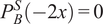 ,
$ {P}_B^S\left(-x\right)=0 $
,
$ {P}_B^S\left(-x\right)=0 $
 , and
$ {P}_B^S(2x)=1 $
, and
$ {P}_B^S(2x)=1 $
 . For
$ q=0 $
. For
$ q=0 $
 and
$ q=x $
and
$ q=x $
 , we have

implying that

and

implying that

Given this pricing rule, the speculator strictly prefers to buy upon learning that
$ A=1 $
 , strictly prefers to short sell upon learning that
$ A=0 $
, strictly prefers to short sell upon learning that
$ A=0 $
 , and strictly prefers to abstain upon learning nothing.
In this case, the speculator’s expected trading profit is

Note that the speculator’s expected trading profit strictly increases with
$ {b}_0 $
 :
:

Moreover, note that

and

Hence, there exists a
$ {\overline{b}}_0^S\in \left(0,1\right) $
 such that
$ {\Pi}_B^S<{\Pi}_0^S\iff {b}_0<{\overline{b}}_0^S $
such that
$ {\Pi}_B^S<{\Pi}_0^S\iff {b}_0<{\overline{b}}_0^S $
 .
.
Funding statement
This research has benefited from financial support from the Swedish House of Finance, the Jan Wallander and Tom Hedelius Foundation, and the Tore Browaldh Foundation.



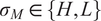







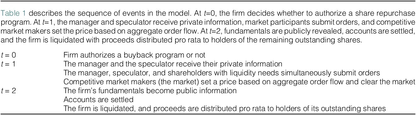
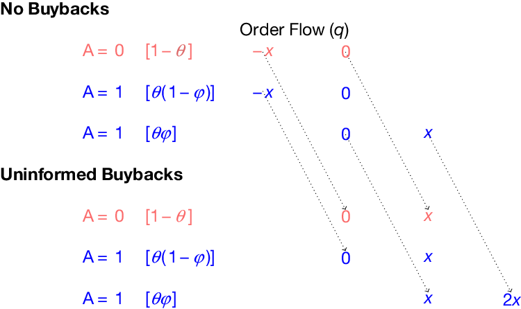


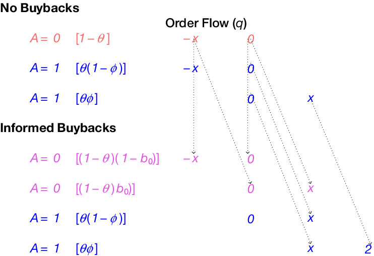


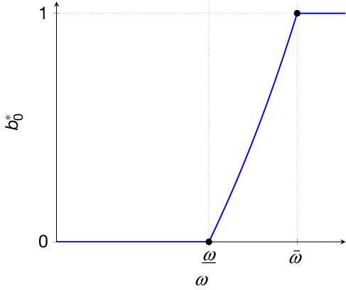









 Open access

