


1. Introduction
Spatial pressure gradients cause turbulent boundary layers (TBLs) to significantly deviate from their canonical behaviours, intensifying the challenges in understanding and predicting turbulent flows to optimise performance and efficiency of engineering systems. Many investigations have probed the effects of the sign (favourable/adverse), strength and history of pressure gradients on TBL response. Summaries of the current state of understanding can be found in Parthasarathy (Reference Parthasarathy2023a ), Harun (Reference Harun2012) and Balin (Reference Balin2020). In many engineering scenarios, however, pressure gradients vary in time as well as in space. For example, manoeuvring aircraft experience time-varying pressure fields due to changes in angle of attack or vehicle acceleration/deceleration. Vehicles operating in gusty weather conditions encounter sudden temporal changes in pressure gradients due to fluctuations in atmospheric turbulence. In rotating machinery, such as turbines and compressors, blades experience dynamically changing spatial pressure gradients. These factors further complicate the physics, and the governing parametric space expands to additionally include the type (periodic pulsating/non-periodic transient), magnitude and time scale of unsteadiness. Despite their practical relevance, unsteady pressure gradient (UPG) TBLs have received limited attention, mainly due to the following challenges: (i) complexity in generating these conditions repeatably in experiments or cheaply in simulations; (ii) cost of collecting and managing large volumes of data necessary for good statistics; (iii) difficulty in separating the effects of unsteadiness and pressure gradients, especially when pressure gradient effects are also not well-understood. The present work attempts to tackle these challenges to provide some insights into the effect of unsteadiness on TBLs under spatial pressure gradients. A brief review of the literature follows.
Early experimental studies on periodic unsteady TBLs, created by oscillating the free stream or using mechanically oscillating surfaces, reported that for a wide range of forcing magnitudes and time scales, the time-averaged turbulent quantities were similar to that of the corresponding steady mean pressure gradient, suggesting that the effect of unsteadiness on the pressure gradient response was only mild. These studies are reviewed in Carr (Reference Carr1981). Reduced frequency, $k$
, defined as the ratio of convective time scale (
$k$
, defined as the ratio of convective time scale ( $t_c$
) to the time scale of imposed unsteadiness (
$t_c$
) to the time scale of imposed unsteadiness ( $t_f$
), varied in [0–85]. Here
$t_f$
), varied in [0–85]. Here $t_c$
is typically computed from the free stream velocity and a reference length scale: chord length for airfoils, boundary layer development length for flat-plate TBLs. Here
$t_c$
is typically computed from the free stream velocity and a reference length scale: chord length for airfoils, boundary layer development length for flat-plate TBLs. Here $t_f$
is the inverse of frequency for periodic forcing, or the total unsteady time for transient forcing. Brereton et al. (Reference Brereton, Reynolds and Jayaraman1990) reasoned that turbulence being a broadband phenomenon, a single excitation frequency cannot strongly affect its average behaviour unless that frequency happened to cause ‘resonance of some kind’. Significant unsteady effects have been observed in phase-averaged turbulent quantities, however, whenever
$t_f$
is the inverse of frequency for periodic forcing, or the total unsteady time for transient forcing. Brereton et al. (Reference Brereton, Reynolds and Jayaraman1990) reasoned that turbulence being a broadband phenomenon, a single excitation frequency cannot strongly affect its average behaviour unless that frequency happened to cause ‘resonance of some kind’. Significant unsteady effects have been observed in phase-averaged turbulent quantities, however, whenever $k \gt$
0.1. Covert & Lorber (Reference Covert and Lorber1984) subjected an airfoil TBL to free stream oscillations with a mean adverse pressure gradient (APG) at
$k \gt$
0.1. Covert & Lorber (Reference Covert and Lorber1984) subjected an airfoil TBL to free stream oscillations with a mean adverse pressure gradient (APG) at $k$
= 0.5, 1, 2 and 6.4. They observed phase lags and leads in the outer and inner regions, respectively, of the ensemble-averaged mean, and the Reynolds stresses seemed to depend more strongly on the mean pressure gradient than on the reduced frequency. When the mean APG was strong enough to cause incipient separation, interestingly, the effect of increasing
$k$
= 0.5, 1, 2 and 6.4. They observed phase lags and leads in the outer and inner regions, respectively, of the ensemble-averaged mean, and the Reynolds stresses seemed to depend more strongly on the mean pressure gradient than on the reduced frequency. When the mean APG was strong enough to cause incipient separation, interestingly, the effect of increasing $k$
on the mean velocity was found to be equivalent to prescribing a less-APG.
$k$
on the mean velocity was found to be equivalent to prescribing a less-APG.
Pronounced unsteady effects in separating TBLs under periodic UPGs have been observed by several other researchers (Ambrogi et al. Reference Ambrogi, Piomelli and Rival2022), as well as the inability of low-fidelity simulations in accurately predicting these effects (Sengupta & Tucker Reference Sengupta and Tucker2020). Park et al. (Reference Park, Ha and You2021) analysed the predictive capability of unsteady Reynolds-averaged Navier–Stokes in a domain with periodic blowing and suction imposed on a flat-plate TBL. By comparing with direct numerical simulation (DNS) results, the unsteady Reynolds-averaged Navier–Stokes simulations with two industry-standard turbulence models were shown to predict erroneously several aspects of TBL separation and reattachment, while their predictions for a corresponding steady pressure gradient were found to be satisfactory. It was also highlighted that the phase-averaged statistics of the unsteady flow showed different features than the time-averaged statistics of the corresponding steady flow. A successful scaling of phase-averaged statistics in space and in time was achieved by Schatzman & Thomas (Reference Schatzman and Thomas2017) in their experimental study of unsteady APG TBLs under conditions relevant to helicopter dynamic stall ( $k$
= 0.12 in their experiments). They identified that the flow physics were dominated by the existence of an embedded shear layer. A collapse was achieved when scaling parameters relevant to the embedded shear layer were employed.
$k$
= 0.12 in their experiments). They identified that the flow physics were dominated by the existence of an embedded shear layer. A collapse was achieved when scaling parameters relevant to the embedded shear layer were employed.
Studies on non-periodic/transient UPG forcing are limited compared with their periodic counterpart, while many advances have been made in the study of transient pipe/channel flows. These are relevant and useful to the transient TBL problem due to the fundamental similarities across wall-bounded flows (Monty et al. Reference Monty, Hutchins, Ng, Marusic and Chong2009). By executing a rapid change in flow rate, a transient acceleration or deceleration of pipe/channel flow has been achieved, and the temporal evolution of turbulence has been tracked. Distinct stages of delays in the flow response, associated with turbulence production, redistribution and radial propagation, have been identified (He & Jackson Reference He and Jackson2000; Seddighi et al. Reference Seddighi, He, Orlandi and Vardy2011; Guerrero et al. Reference Guerrero, Lambert and Chin2021). The delays have been reported to cause the ensemble-averaged statistics to over- and under-shoot the corresponding steady-state statistics. The time scales at which the processes occur have also been distilled. Such characterisations have helped improve unsteady friction modelling in pipes and channels, which is of great practical importance. Similarities between temporally developing internal/external flows and spatially developing internal/external flows have been noted in the literature. Mathur et al. (Reference Mathur, Gorji, He, Seddighi, Vardy, O’Donoghue and Pokrajac2018) reported in their work that rapidly accelerated channel flows showed similar features as relaminarising favourable pressure gradient (FPG) TBLs. By numerically studying a flat-plate TBL rapidly accelerated from Mach number 0.3–0.6 in 10 ms and 25 ms, Saavedra et al. (Reference Saavedra, Poggie and Paniagua2020) observed stages of acceleration (inertia-dominated stage followed by relaxation due to viscous diffusion) that were qualitatively similar to those identified in rapidly accelerated pipes/channels. Saavedra & Paniagua (Reference Saavedra and Paniagua2021) studied the effects of a sudden flow acceleration over a wall-mounted hump (FPG–APG sequence), in the compressible subsonic flow regime. They noted a boost of near-wall momentum due to the sudden acceleration, enough for the TBL to overcome APG-induced flow detachment, suggesting that mean flow transients can be leveraged to modulate separation events. In a computational study by Kharghani & PasandidehFard (Reference Kharghani and PasandidehFard2022), a flat-plate TBL under a FPG–APG sequence was created using a converging–diverging slip-wall and was temporally accelerated. Under the combined stabilising influence of temporal acceleration and the FPG, turbulent stresses were strongly suppressed, especially in the wall-normal direction, and the TBL was found to become laminarescent. In the succeeding APG region, the boundary layer retransitioned and the APG was observed to aid a redistribution of turbulent energy among its components, despite the continued temporal acceleration.
The objective of this paper is to report on the spatiotemporal statistics and the structure of a TBL experiencing an UPG. Since the effects of unsteadiness and pressure gradients are highly coupled, comparisons are made at discrete time instances with equivalent (matched in magnitude) steady pressure gradients. The paper is organised as follows. The experimental facility used to impose the required steady and unsteady TBLs, the test parameters and measurement methods are described in § 2. In § 3, the results are presented in terms of the mean and Reynolds stresses, statistics of vortex organisation, spectral content of the flow and coherent structures derived from proper orthogonal decompositions (PODs). The steady pressure gradient cases have already been analysed and discussed in Parthasarathy & Saxton-Fox (Reference Parthasarathy and Saxton-Fox2023). Relevant summaries from this analysis are also provided in this section before presenting the unsteady effects. The results are discussed and a hypothesis for the observed behaviours is provided in § 5. Section 6 concludes the paper.
2. Experimental methodology
The experiments were carried out in a low-speed, subsonic, open-return boundary layer wind tunnel at the University of Illinois’ Aerodynamics Research Laboratory (Rodriguez Reference Rodriguez2020). The dimensions of the test section are $0.381\,\rm m$ $\times$ $0.381\,\rm m$ $\times$ $3.657\,\rm m$
(
$3.657\,\rm m$
( $15''$ $\times$ $15''$ $\times$ $12'$
). The boundary layer of interest is developed over a
$12'$
). The boundary layer of interest is developed over a $2.54\,\rm cm$
-thick flat plate extending the entire length of the test section. A sandpaper strip of 5 cm width and grit size 40 is affixed at the leading edge to trip the boundary layer to turbulent. A nominally zero pressure gradient (ZPG) TBL develops over a distance of
$2.54\,\rm cm$
-thick flat plate extending the entire length of the test section. A sandpaper strip of 5 cm width and grit size 40 is affixed at the leading edge to trip the boundary layer to turbulent. A nominally zero pressure gradient (ZPG) TBL develops over a distance of $2.35\,\rm m$
before reaching the
$2.35\,\rm m$
before reaching the $0.61\,\rm m$
long test area where the pressure gradients are created and the TBL is studied. A computer rendering of this facility is shown in figure 1(a). The red dashed box denotes the test area and the ceiling components at that location illustrate the UPG installation used to generate the pressure gradients.
$0.61\,\rm m$
long test area where the pressure gradients are created and the TBL is studied. A computer rendering of this facility is shown in figure 1(a). The red dashed box denotes the test area and the ceiling components at that location illustrate the UPG installation used to generate the pressure gradients.
Illustration of the experimental details. (a) The BLWT and the UPG installation. The red box bounds the test area. (b) Close-up view of the test area where the flat plate TBL experiences the pressure gradients. Here $D_c$
is the instantaneous vertical distance travelled by the midpoint of the deforming ceiling. The field of view(FOV) for particle image velocimetry(PIV) is set in the APG region of the test area. Note that coordinate systems [x,y] and [x′,y′] are used to define locations with respect to the PIV FOV and the ceiling panel, respectively. (c) Ceiling deformation speed is defined as the constant speed of the ceiling midpoint. (d) Ensemble-averaged unsteady TBL mean is shown at the start and end of UPG imposition.
$D_c$
is the instantaneous vertical distance travelled by the midpoint of the deforming ceiling. The field of view(FOV) for particle image velocimetry(PIV) is set in the APG region of the test area. Note that coordinate systems [x,y] and [x′,y′] are used to define locations with respect to the PIV FOV and the ceiling panel, respectively. (c) Ceiling deformation speed is defined as the constant speed of the ceiling midpoint. (d) Ensemble-averaged unsteady TBL mean is shown at the start and end of UPG imposition.
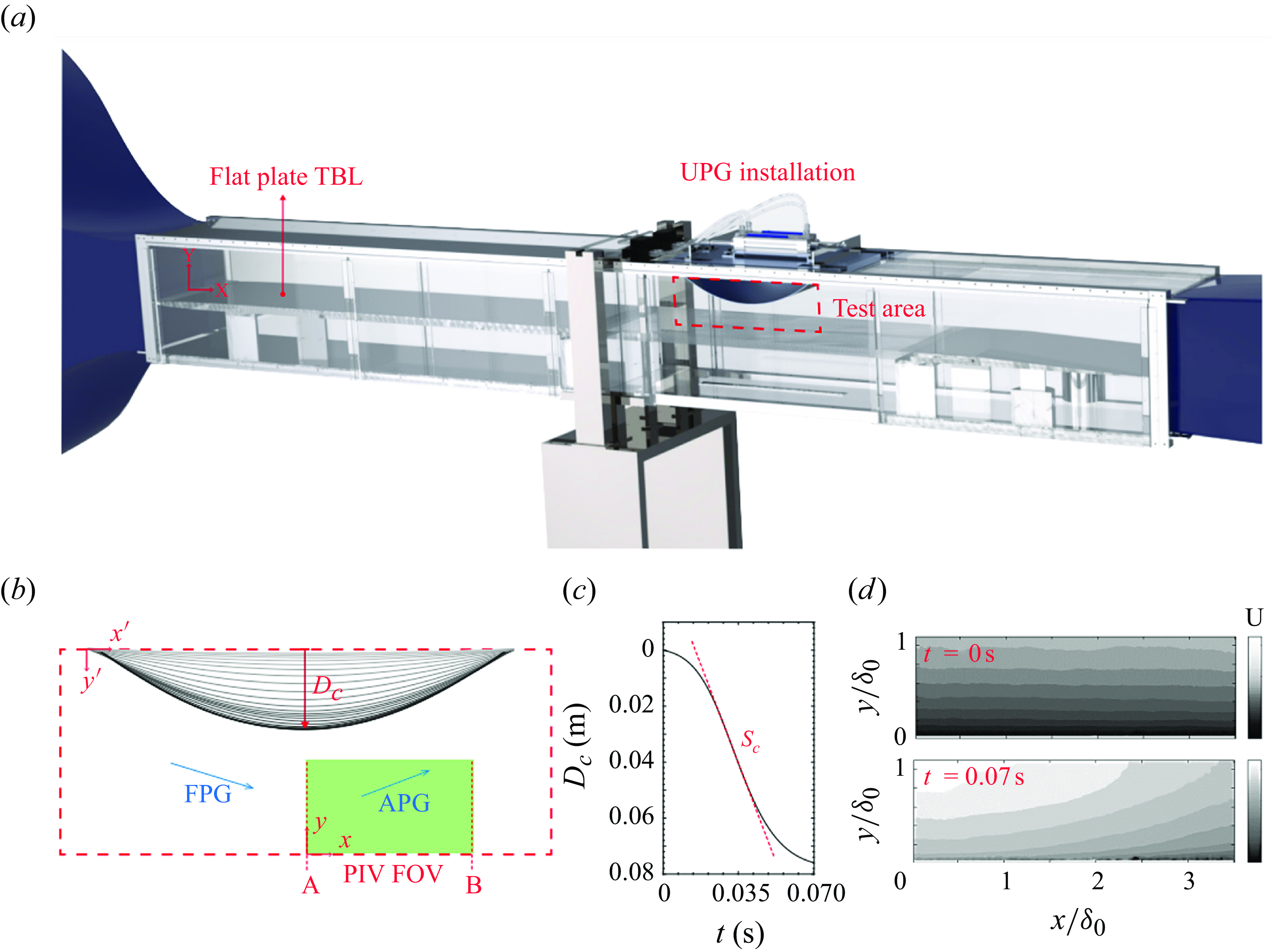
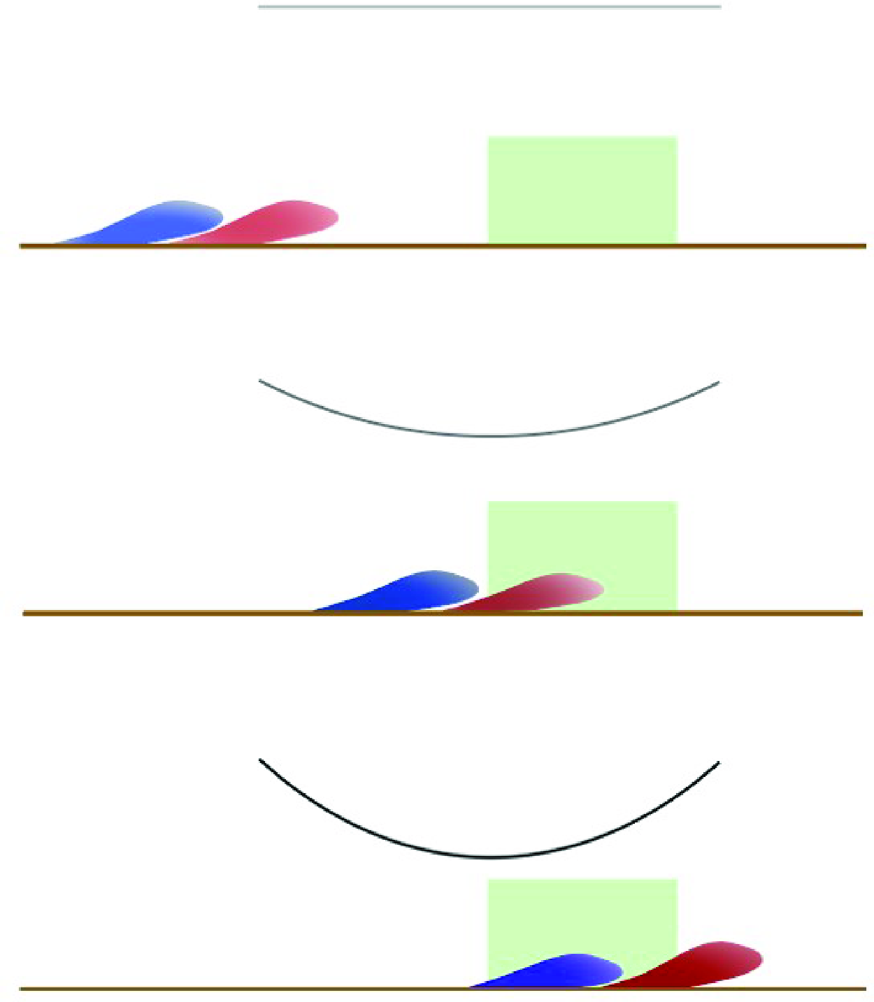
The installation includes the following: (i) a flexible false ceiling panel that sits within the test section and forms the ceiling of the test area, (ii) two linear actuators that sit outside the test section and (iii) mechanical linkages that connect the actuator rods to the streamwise edges of the flexible panel. The two actuators are controlled by two electropneumatic valves that take input via a computer programming interface (LabVIEW). When the actuator rods are made to retract, the flat ceiling panel deforms to an inverted convex bump shape. The ceiling bump imposes a spatial pressure gradient sequence of favourable followed by adverse on the flat-plate TBL, and as the bump’s curvature temporally increases, the spatial pressure gradient sequence imposed strengthens with time. The dynamically changing ceiling geometries are illustrated in figure 1(b). The profiles are extracted from high-speed images of the deforming ceiling, the details of which can be found in Parthasarathy & Saxton-Fox (Reference Parthasarathy and Saxton-Fox2022), along with a detailed description of the facility and its characterisation. Note that an opposite one-way deformation of the panel, from curved to flat such that the spatial pressure gradient weakens in time, would result in a different flow response and is of interest for future work. Here $D_c$
, marked in the figure, quantifies the vertical deformation height of the midpoint of the ceiling panel and governs the spatial strength of the favourable to adverse pressure gradient (FAPG) imposed. Higher
$D_c$
, marked in the figure, quantifies the vertical deformation height of the midpoint of the ceiling panel and governs the spatial strength of the favourable to adverse pressure gradient (FAPG) imposed. Higher $D_c$
corresponds to stronger FAPG strength. The speed of deformation,
$D_c$
corresponds to stronger FAPG strength. The speed of deformation, $S_c$
, is obtained as the slope of the
$S_c$
, is obtained as the slope of the $D_c$
–
$D_c$
– $t$
plot of the midpoint, as shown in figure 1(c). Here
$t$
plot of the midpoint, as shown in figure 1(c). Here $t$
is the instantaneous time. Here
$t$
is the instantaneous time. Here $S_c$
governs the pressure gradient time scale or its dynamic strength. Higher
$S_c$
governs the pressure gradient time scale or its dynamic strength. Higher $S_c$
corresponds to lower unsteady time scales and a more dynamic imposed FAPG. The ceiling deformation can also be held statically (
$S_c$
corresponds to lower unsteady time scales and a more dynamic imposed FAPG. The ceiling deformation can also be held statically ( $S_c$
= 0) at different
$S_c$
= 0) at different $D_c$
, thus creating the same spatial FAPGs without the unsteadiness. By comparing the TBL’s response with the unsteady FAPG application with its responses to a series of steady FAPG applications, which were separately studied in Parthasarathy & Saxton-Fox (Reference Parthasarathy and Saxton-Fox2023), the effects of unsteadiness are isolated from the effects of the spatial pressure gradients, which are both simultaneously present in the unsteady case.
$D_c$
, thus creating the same spatial FAPGs without the unsteadiness. By comparing the TBL’s response with the unsteady FAPG application with its responses to a series of steady FAPG applications, which were separately studied in Parthasarathy & Saxton-Fox (Reference Parthasarathy and Saxton-Fox2023), the effects of unsteadiness are isolated from the effects of the spatial pressure gradients, which are both simultaneously present in the unsteady case.
In the present study, $D_c$
was set to span [1–76
$D_c$
was set to span [1–76 $\rm mm$
]. In the unsteady case, the range was spanned dynamically in 0.07 s by performing a deflect and hold manoeuvre of the ceiling panel, and in the steady cases, the panel was held at 22 discrete deformations within the chosen range. The maximum deflection of
$\rm mm$
]. In the unsteady case, the range was spanned dynamically in 0.07 s by performing a deflect and hold manoeuvre of the ceiling panel, and in the steady cases, the panel was held at 22 discrete deformations within the chosen range. The maximum deflection of $D_c$
= 76
$D_c$
= 76 $\rm mm$
corresponds to a minimum area ratio (
$\rm mm$
corresponds to a minimum area ratio ( $A_m/A_0$
) of 40
$A_m/A_0$
) of 40 $\, \%$
, where
$\, \%$
, where $A$
is the cross-sectional area local to a streamwise location and
$A$
is the cross-sectional area local to a streamwise location and $A_0$
is the cross-sectional area upstream of the test area. Here
$A_0$
is the cross-sectional area upstream of the test area. Here $S_c$
was chosen to be 1.5 ms−1 in the unsteady case. The dynamic strength of this pressure gradient imposition can be quantified in several ways. One dimensionless quantity is the inertial reduced frequency,
$S_c$
was chosen to be 1.5 ms−1 in the unsteady case. The dynamic strength of this pressure gradient imposition can be quantified in several ways. One dimensionless quantity is the inertial reduced frequency, $k_x \equiv t_c/t_f$
, defined as the ratio of convective time scale to imposed unsteady time scale, which equalled 4.38. The convective time scale,
$k_x \equiv t_c/t_f$
, defined as the ratio of convective time scale to imposed unsteady time scale, which equalled 4.38. The convective time scale, $t_c$
, has been computed using the free stream velocity and the boundary layer development length over the flat plate. The unsteady time scale,
$t_c$
, has been computed using the free stream velocity and the boundary layer development length over the flat plate. The unsteady time scale, $t_f$
, is the time over which the UPG is applied (
$t_f$
, is the time over which the UPG is applied ( $=$
0.07 s). Note that although reduced frequencies are more commonly defined in studies on periodic unsteadiness, the current UPG imposition is transient. Another dimensionless quantity to characterise the dynamic nature of the pressure gradient is the turbulent reduced frequency,
$=$
0.07 s). Note that although reduced frequencies are more commonly defined in studies on periodic unsteadiness, the current UPG imposition is transient. Another dimensionless quantity to characterise the dynamic nature of the pressure gradient is the turbulent reduced frequency, $k_\tau \equiv t_\tau / t_f$
, where
$k_\tau \equiv t_\tau / t_f$
, where $t_\tau$
is the large turbulent time scale defined as
$t_\tau$
is the large turbulent time scale defined as $t_\tau \equiv \delta _0/u_{\tau _0}$
(Momen & Bou-Zeid Reference Momen and Bou-Zeid2017) where
$t_\tau \equiv \delta _0/u_{\tau _0}$
(Momen & Bou-Zeid Reference Momen and Bou-Zeid2017) where $k_\tau$
= 1.79 in this study. Finally, the characteristic deformation speed can be directly compared with the incoming free stream speed,
$k_\tau$
= 1.79 in this study. Finally, the characteristic deformation speed can be directly compared with the incoming free stream speed, $S^* \equiv S_c/U_0$
. This ratio was 0.19 for the case considered here.
$S^* \equiv S_c/U_0$
. This ratio was 0.19 for the case considered here.
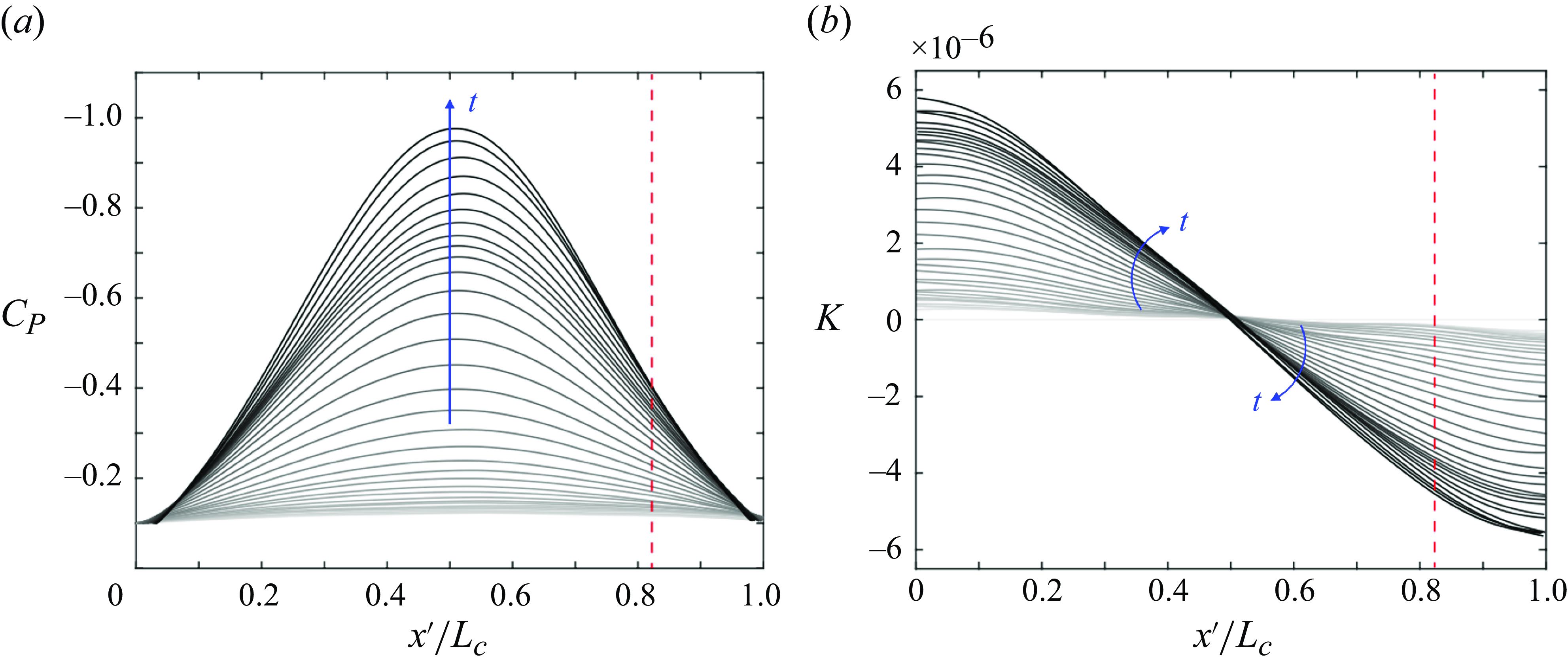
The temporally varying spatial distributions of the non-dimensional pressure coefficient, $C_P$
, created in the test area due to the deforming ceiling are shown in figure 2(a). The profiles were computed analytically with incompressible, inviscid external flow assumption, using the exact geometric states of the ceiling, and were experimentally validated to be accurate within
$C_P$
, created in the test area due to the deforming ceiling are shown in figure 2(a). The profiles were computed analytically with incompressible, inviscid external flow assumption, using the exact geometric states of the ceiling, and were experimentally validated to be accurate within $6\, \%$
using high-frequency pressure measurements (Parthasarathy & Saxton-Fox Reference Parthasarathy and Saxton-Fox2022). The pressure gradient distributions are shown in figure 2(b) in terms of the acceleration parameter,
$6\, \%$
using high-frequency pressure measurements (Parthasarathy & Saxton-Fox Reference Parthasarathy and Saxton-Fox2022). The pressure gradient distributions are shown in figure 2(b) in terms of the acceleration parameter, $K$
(
$K$
( $\equiv {\nu }/{U_l^2}\;{{\rm d}U_l}/{{\rm d}x}$
, where
$\equiv {\nu }/{U_l^2}\;{{\rm d}U_l}/{{\rm d}x}$
, where $U_l$
is the local average velocity outside the boundary layer). In
$U_l$
is the local average velocity outside the boundary layer). In $0\lt x'/L_c\lt 0.5$
, the pressure gradient is favourable, and in
$0\lt x'/L_c\lt 0.5$
, the pressure gradient is favourable, and in $0.5\lt x'/L_c\leqslant 0.82$
, the pressure gradient is adverse. The overall FAPG strength increases with time (denoted by darker profiles), as can be expected. The flow over the ceiling panel was found to have separated in
$0.5\lt x'/L_c\leqslant 0.82$
, the pressure gradient is adverse. The overall FAPG strength increases with time (denoted by darker profiles), as can be expected. The flow over the ceiling panel was found to have separated in $x/L\gt 0.82$
, marked by the red dashed line, rendering the pressure distributions invalid after this point (Parthasarathy & Saxton-Fox Reference Parthasarathy and Saxton-Fox2022). For the 22 steady FAPG impositions that were measured, the pressure gradient distributions matched specific time instances of the unsteady distributions shown in figure 2(b). The matched steady distributions can be found in Parthasarathy & Saxton-Fox (Reference Parthasarathy and Saxton-Fox2023), where the physics of the TBL’s response to the steady FAPGs has been discussed.
$x/L\gt 0.82$
, marked by the red dashed line, rendering the pressure distributions invalid after this point (Parthasarathy & Saxton-Fox Reference Parthasarathy and Saxton-Fox2022). For the 22 steady FAPG impositions that were measured, the pressure gradient distributions matched specific time instances of the unsteady distributions shown in figure 2(b). The matched steady distributions can be found in Parthasarathy & Saxton-Fox (Reference Parthasarathy and Saxton-Fox2023), where the physics of the TBL’s response to the steady FAPGs has been discussed.
(a) Coefficient of pressure distributions caused by different geometric states of the ceiling. Darker greys correspond to more deformed ceiling states (higher $D_c$
) which occur later in time. (b) Corresponding pressure gradient distributions, shown in terms of the acceleration parameter,
$D_c$
) which occur later in time. (b) Corresponding pressure gradient distributions, shown in terms of the acceleration parameter, $K$
. The red dashed line indicates the location of flow separation from the ceiling.
$K$
. The red dashed line indicates the location of flow separation from the ceiling.
The response of the boundary layer to the unsteady ceiling motion in the APG region that is downstream of the FPG region is the focus of the present study. The spatiotemporal response of the TBL to the unsteady FAPG imposition was captured using time-resolved PIV in the streamwise wall-normal plane located at the midspan of the flat plate. The FOV of size $150 \times 93.75\,\rm mm$
(
$150 \times 93.75\,\rm mm$
( $L_x \times L_y$
,
$L_x \times L_y$
, $3.57\delta _0 \times 2.23\delta _0$
) is illustrated in figure 2(b). Mineral-oil-based seeding particles were introduced at the inlet of the tunnel. The FOV was illuminated by a laser sheet of 1 mm depth, formed using a Terra PIV 527-80-M double-pulsed laser. A Phantom VEO 710L camera was used with a Nikon
$3.57\delta _0 \times 2.23\delta _0$
) is illustrated in figure 2(b). Mineral-oil-based seeding particles were introduced at the inlet of the tunnel. The FOV was illuminated by a laser sheet of 1 mm depth, formed using a Terra PIV 527-80-M double-pulsed laser. A Phantom VEO 710L camera was used with a Nikon $50\,\rm mm$
lens at
$50\,\rm mm$
lens at $f$
/1.8 to capture the particle images in a frame-straddling mode. The windows, floor and ceiling around the test area were blackened using matte black spray paint to reduce reflections, leaving just the necessary regions for the laser sheet to enter the test section and for the camera to image the FOV.
$f$
/1.8 to capture the particle images in a frame-straddling mode. The windows, floor and ceiling around the test area were blackened using matte black spray paint to reduce reflections, leaving just the necessary regions for the laser sheet to enter the test section and for the camera to image the FOV.
For the unsteady case, the data were acquired in a phase-locked, time-resolved manner. The data rate was set at 3.755 kHz, and the recording time was 0.091 s. The time between two frames, $\Delta t$
= 90
$\Delta t$
= 90 $\,\unicode{x03BC} \textrm{s}$
, to allow roughly seven pixels displacement of particles between frames. Furthermore, 400 independent ensembles of data were acquired by performing 400 transient deformations of the ceiling, allowing sufficient time between each deformation for the flow to recover. The 400 tests allowed the computation of ensemble-averaged time-varying statistics of the unsteady flow. The phase-matching across ensembles was achieved by carefully synchronising the ceiling motion and the PIV data acquisition. An external trigger (5V TTL) was generated in LabVIEW to signal the start of the ceiling deformation and sent to a LaVision Programmable Timing Unit. The LaVision Programmable Timing Unit managed the synchronisation between the camera and the laser. An ending trigger was sent at t = 1.3
$\,\unicode{x03BC} \textrm{s}$
, to allow roughly seven pixels displacement of particles between frames. Furthermore, 400 independent ensembles of data were acquired by performing 400 transient deformations of the ceiling, allowing sufficient time between each deformation for the flow to recover. The 400 tests allowed the computation of ensemble-averaged time-varying statistics of the unsteady flow. The phase-matching across ensembles was achieved by carefully synchronising the ceiling motion and the PIV data acquisition. An external trigger (5V TTL) was generated in LabVIEW to signal the start of the ceiling deformation and sent to a LaVision Programmable Timing Unit. The LaVision Programmable Timing Unit managed the synchronisation between the camera and the laser. An ending trigger was sent at t = 1.3 $t_f$
, where 5 s were allowed to pass before starting over. More details on the timing and synchronisation can be found in Parthasarathy (Reference Parthasarathy2023b
).
$t_f$
, where 5 s were allowed to pass before starting over. More details on the timing and synchronisation can be found in Parthasarathy (Reference Parthasarathy2023b
).
For each of the 22 steady cases, both time-resolved and non-time-resolved data were recorded: 6170 particle image pairs in a single recording at 3.755 kHz in the former, and 10,000 image pairs at 0.2 kHz in the latter, with $\Delta t = 90$ $\unicode{x03BC} s$
, as before. The particle image pairs from the steady and unsteady tests were processed using a multipass approach with the final interrogation window size of
$\unicode{x03BC} s$
, as before. The particle image pairs from the steady and unsteady tests were processed using a multipass approach with the final interrogation window size of $16 \times 16$
. The resulting vector fields had a spatial resolution of
$16 \times 16$
. The resulting vector fields had a spatial resolution of $\Delta l^+$
= 8.9, and the time-resolved fields also had a temporal resolution of
$\Delta l^+$
= 8.9, and the time-resolved fields also had a temporal resolution of $\Delta t^+$
= 1.8. The kinematic viscosity,
$\Delta t^+$
= 1.8. The kinematic viscosity, $\nu$
, and the friction velocity of the ZPG case,
$\nu$
, and the friction velocity of the ZPG case, $u_{\tau _0}$
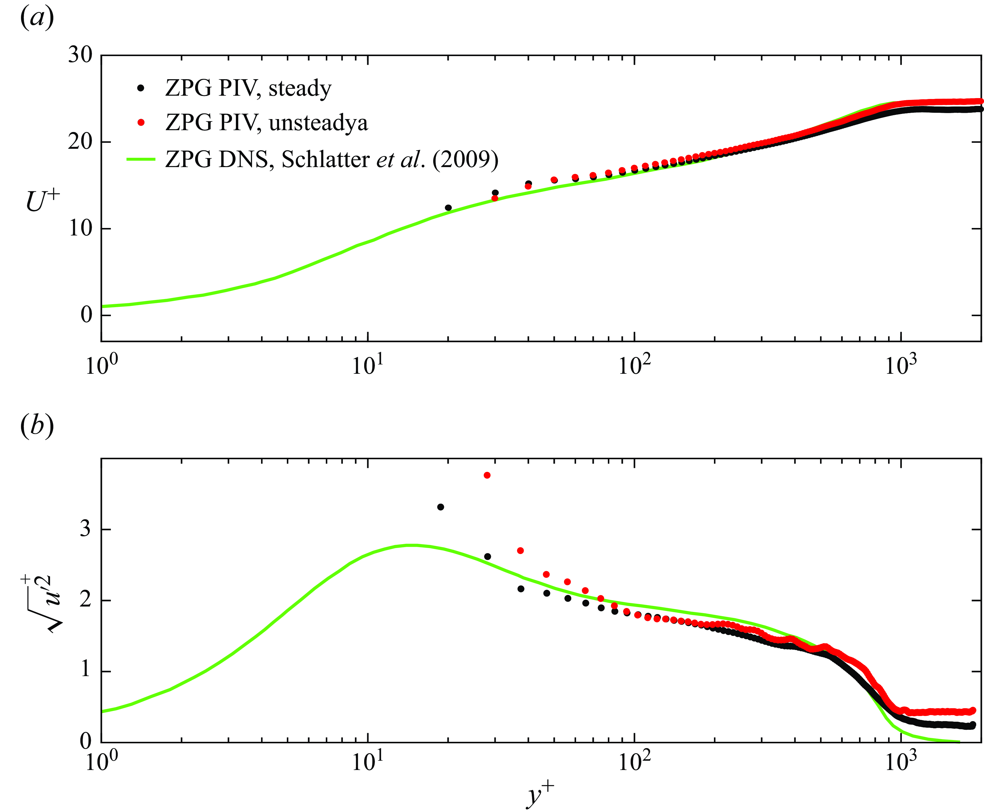
, were used in defining the viscous scales. A comparison of the measured ZPG mean and streamwise root mean square (r.m.s.) velocity with DNS of Schlatter et al. (Reference Schlatter, Örlü, Li, Brethouwer, Fransson, Johansson, Alfredsson and Henningson2009) is shown in figure 3, computed from both the steady and unsteady data. For the steady case, 6170 time-correlated data have been time-averaged with the ceiling held flat, and for the unsteady case, 400 ensembles of data have been ensemble-averaged at
$u_{\tau _0}$
, were used in defining the viscous scales. A comparison of the measured ZPG mean and streamwise root mean square (r.m.s.) velocity with DNS of Schlatter et al. (Reference Schlatter, Örlü, Li, Brethouwer, Fransson, Johansson, Alfredsson and Henningson2009) is shown in figure 3, computed from both the steady and unsteady data. For the steady case, 6170 time-correlated data have been time-averaged with the ceiling held flat, and for the unsteady case, 400 ensembles of data have been ensemble-averaged at $t_f = 0$
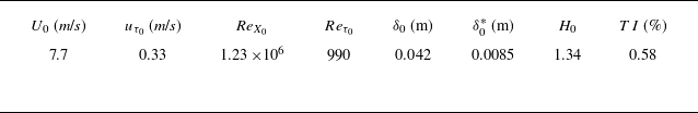
. The wind tunnel conditions relevant to the current tests are summarised in table 1, all measured at the centre of the PIV FOV from the acquired data. Listed in the table are the ZPG conditions, including free stream velocity,
$t_f = 0$
. The wind tunnel conditions relevant to the current tests are summarised in table 1, all measured at the centre of the PIV FOV from the acquired data. Listed in the table are the ZPG conditions, including free stream velocity, $U_0$
,
$U_0$
, $99\, \%$
boundary layer thickness,
$99\, \%$
boundary layer thickness, $\delta _0$
, displacement thickness,
$\delta _0$
, displacement thickness, $\delta _0^*$
, free stream turbulence intensity,
$\delta _0^*$
, free stream turbulence intensity, $TI$
, ZPG case (Clauser Reference Clauser1956).
$TI$
, ZPG case (Clauser Reference Clauser1956).
Comparison of measured mean velocity and streamwise r.m.s. velocity from PIV to benchmark DNS data, all at ZPG conditions. The steady profiles have been computed by time-averaging non-time-resolved data with the ceiling statically held flat. The unsteady profiles have been obtained by ensemble-averaging the time-resolved unsteady data at $t_f$
= 0, just before the ceiling starts deforming.
$t_f$
= 0, just before the ceiling starts deforming.
Freestream conditions measured at the centre of the PIV field of view for the ZPG case.
The response of the TBL within the APG region studied is expected to depend not only on the local APG strength shown in figure 2(b), but also on the strength of the upstream FPG shown. This is due to the pressure gradient history effects, as discussed in Parthasarathy & Saxton-Fox (Reference Parthasarathy and Saxton-Fox2023). Both FPG and APG strengths simultaneously change as the ceiling deflection is increased, statically in the steady cases and dynamically in the unsteady case. To quantify this changing overall FAPG strength for different deflections of the ceiling, a spatially averaged pressure gradient variable is defined as $\overline {K}_B$ $\equiv$ ${1}/{x_B - x'_{0}}$ $\int _{x'_{0}}^{x_B} K(x) \,{\rm d}x$
. Here
$\int _{x'_{0}}^{x_B} K(x) \,{\rm d}x$
. Here $x'_{0}$
corresponds to
$x'_{0}$
corresponds to $x'/L_c$
= 0, the beginning of the FPG region, and
$x'/L_c$
= 0, the beginning of the FPG region, and $x_B$
corresponds to
$x_B$
corresponds to $x/L_x$
= 1, the last station of the PIV FOV (marked as
$x/L_x$
= 1, the last station of the PIV FOV (marked as $B$
in figure 1
b). For the 22 deflections of the ceiling when the FAPG strengths are instantaneously matched between the steady and unsteady cases,
$B$
in figure 1
b). For the 22 deflections of the ceiling when the FAPG strengths are instantaneously matched between the steady and unsteady cases, $\overline {K}_B \times 10^6$
= [0; 0.11; 0.16; 0.18; 0.25; 0.30; 0.40; 0.45; 0.50; 0.55; 0.60; 0.67; 0.73; 0.77; 0.84; 0.90; 0.96; 1.03; 1.12; 1.17; 1.19; 1.20], in the order of increasing
$\overline {K}_B \times 10^6$
= [0; 0.11; 0.16; 0.18; 0.25; 0.30; 0.40; 0.45; 0.50; 0.55; 0.60; 0.67; 0.73; 0.77; 0.84; 0.90; 0.96; 1.03; 1.12; 1.17; 1.19; 1.20], in the order of increasing $D_c$
or FAPG strength. For the sake of compactness,
$D_c$
or FAPG strength. For the sake of compactness, $\overline {K}_B \times 10^6$
is renamed as
$\overline {K}_B \times 10^6$
is renamed as $\bar {K}$
. Here
$\bar {K}$
. Here $\bar {K}$
is similar to the average Clauser pressure gradient parameter
$\bar {K}$
is similar to the average Clauser pressure gradient parameter $\bar {\beta }$
introduced by Vinuesa et al. (Reference Vinuesa, Örlü, Sanmiguel Vila, Ianiro, Discetti and Schlatter2017). While
$\bar {\beta }$
introduced by Vinuesa et al. (Reference Vinuesa, Örlü, Sanmiguel Vila, Ianiro, Discetti and Schlatter2017). While $\bar {\beta }$
was meant to capture the pressure gradient history in that non-equilibrium APG flow, that is not the intention with
$\bar {\beta }$
was meant to capture the pressure gradient history in that non-equilibrium APG flow, that is not the intention with $\bar {K}$
. A single value that correctly signifies the strength and/or history of the pressure gradient is a topic of ongoing work even for single-signed pressure gradients, and sign changes in the pressure gradient complicates it further. Therefore, the intention with
$\bar {K}$
. A single value that correctly signifies the strength and/or history of the pressure gradient is a topic of ongoing work even for single-signed pressure gradients, and sign changes in the pressure gradient complicates it further. Therefore, the intention with $\bar {K}$
is to use a physically relevant parameter to refer to the overall FAPG strength for different deflections of the ceiling, not to universalise behaviour based on
$\bar {K}$
is to use a physically relevant parameter to refer to the overall FAPG strength for different deflections of the ceiling, not to universalise behaviour based on $\bar {K}$
. Note that the same definition of
$\bar {K}$
. Note that the same definition of $\bar {K}$
is used for both the steady and unsteady cases, except for the unsteady case
$\bar {K}$
is used for both the steady and unsteady cases, except for the unsteady case $\bar {K}$
varies as a function of time and
$\bar {K}$
varies as a function of time and $k_x$
conveys the time scale with which
$k_x$
conveys the time scale with which $\bar {K}$
varies in time. Finding a parameter that simultaneously captures the spatial and temporal FAPG change is not straightforward and will be left for future work.
$\bar {K}$
varies in time. Finding a parameter that simultaneously captures the spatial and temporal FAPG change is not straightforward and will be left for future work.
3. Results
The spatiotemporal changes exhibited by the unsteady TBL are presented and discussed by comparing them with changes exhibited by the series of steady TBLs at matched FAPG magnitudes ( $\bar {K}$
). In doing so, an understanding of if and how the dynamic pressure gradient imposition alters the boundary layer’s response to the spatial pressure gradients is sought. The response is studied in terms of the mean, Reynolds stresses, the organisation of vortices in the flow, the turbulent spectrum and energetically dominant modal structures. These results for the series of steady FAPG TBLs have been discussed in detail in Parthasarathy & Saxton-Fox (Reference Parthasarathy and Saxton-Fox2023). In each of the following sections, a brief relevant summary is given, while retaining the focus on the unsteady results. Wherever appropriate, the quantities have been scaled using the edge velocity (
$\bar {K}$
). In doing so, an understanding of if and how the dynamic pressure gradient imposition alters the boundary layer’s response to the spatial pressure gradients is sought. The response is studied in terms of the mean, Reynolds stresses, the organisation of vortices in the flow, the turbulent spectrum and energetically dominant modal structures. These results for the series of steady FAPG TBLs have been discussed in detail in Parthasarathy & Saxton-Fox (Reference Parthasarathy and Saxton-Fox2023). In each of the following sections, a brief relevant summary is given, while retaining the focus on the unsteady results. Wherever appropriate, the quantities have been scaled using the edge velocity ( $U_e$
) and boundary layer thickness (
$U_e$
) and boundary layer thickness ( $\delta$
) local to that space and time, computed using the diagnostic plot technique (Vinuesa et al. Reference Vinuesa, Bobke, Örlü and Schlatter2016).
$\delta$
) local to that space and time, computed using the diagnostic plot technique (Vinuesa et al. Reference Vinuesa, Bobke, Örlü and Schlatter2016).
3.1. Mean and Reynolds stresses
3.1.1. Steady FAPGs
The following observations were noted in Parthasarathy & Saxton-Fox (Reference Parthasarathy and Saxton-Fox2023). The streamwise mean velocity at the exit of the FPG region (i.e. at the beginning of the PIV FOV) exhibited fuller profiles due to the spatial acceleration, and in the succeeding APG (i.e. within the PIV FOV), the flow decelerated from that accelerated state. This was evidenced by a decreasing velocity gradient near the wall. However, the profiles remained significantly more full away from the wall at all stations. This upstream FPG effect on the APG region grew stronger for higher $\bar {K}$
(stronger FAPG), resulting in the mean at the last APG station recorded to become fuller with
$\bar {K}$
(stronger FAPG), resulting in the mean at the last APG station recorded to become fuller with $\bar {K}$
, despite that station locally experiencing a stronger APG at higher
$\bar {K}$
, despite that station locally experiencing a stronger APG at higher $\bar {K}$
. This coupled mean structure was already indicative of the strongly altered turbulence, given the vital role that mean gradients play in setting up turbulence. Accordingly, the streamwise, wall-normal and shear Reynolds stresses showed a bimodal structure coming out of the spatially varying FPG, contrary to a single outer peak structure expected under an APG. The first peak of the bimodal structure showed significant growth as the flow advanced through the APG region, while the second peak showed a decay, particularly for stronger FAPG impositions. These were signatures of an internal boundary layer within the TBL, formed due to the rapid spatial changes in the pressure gradients imposed. The presence and growth of this layer and its effects on other turbulence quantities subsequently studied were found to be significant for FAPG cases where the maximum spatial rate of change of the imposed pressure gradient satisfied
$\bar {K}$
. This coupled mean structure was already indicative of the strongly altered turbulence, given the vital role that mean gradients play in setting up turbulence. Accordingly, the streamwise, wall-normal and shear Reynolds stresses showed a bimodal structure coming out of the spatially varying FPG, contrary to a single outer peak structure expected under an APG. The first peak of the bimodal structure showed significant growth as the flow advanced through the APG region, while the second peak showed a decay, particularly for stronger FAPG impositions. These were signatures of an internal boundary layer within the TBL, formed due to the rapid spatial changes in the pressure gradients imposed. The presence and growth of this layer and its effects on other turbulence quantities subsequently studied were found to be significant for FAPG cases where the maximum spatial rate of change of the imposed pressure gradient satisfied $-({\rm d}K/{\rm d}x)_{max} \delta _0 \geqslant 0.49 \times 10^{-6}$
. For these cases, the internal layer exhibited power law growth within the APG region, with the growth rates linearly increasing from 1.03–2.05 as the overall FAPG strength increased.
$-({\rm d}K/{\rm d}x)_{max} \delta _0 \geqslant 0.49 \times 10^{-6}$
. For these cases, the internal layer exhibited power law growth within the APG region, with the growth rates linearly increasing from 1.03–2.05 as the overall FAPG strength increased.
3.1.2. Unsteady FAPGs
Ensemble-averaged statistics of the unsteady TBL are computed from the time-varying velocity fields that were acquired as the test section ceiling deformed. The outer-scaled mean and Reynolds stresses along the wall-normal direction are presented at six discrete time instances around two $x$
locations, one towards the upstream end of the FOV (marked station
$x$
locations, one towards the upstream end of the FOV (marked station $A$
in figure 1
b) in figure 4, and one towards the downstream end (marked station
$A$
in figure 1
b) in figure 4, and one towards the downstream end (marked station $B$
in figure 1
b) in figure 5. Because the ceiling was deflected from a flat ZPG position to a FAPG deployed position and then held (see figure 1
c for an example deflection trajectory in time), increased time is equivalent to an increase in the magnitude of the local pressure gradient. We therefore use the local value of the spatially averaged pressure gradient,
$B$
in figure 1
b) in figure 5. Because the ceiling was deflected from a flat ZPG position to a FAPG deployed position and then held (see figure 1
c for an example deflection trajectory in time), increased time is equivalent to an increase in the magnitude of the local pressure gradient. We therefore use the local value of the spatially averaged pressure gradient, $\bar {K} = 0$
,
$\bar {K} = 0$
, $0.25$
,
$0.25$
, $0.5$
,
$0.5$
, $0.74$
,
$0.74$
, $0.96$
,
$0.96$
, $1.2$
, as a proxy for time for the unsteady cases. The profiles are shown shifted along the abscissa for clarity. The
$1.2$
, as a proxy for time for the unsteady cases. The profiles are shown shifted along the abscissa for clarity. The $\bar {K}$
is denoted above each profile in the figures in red. The statistics from the corresponding steady pressure gradients, with the ceiling held fixed at the same
$\bar {K}$
is denoted above each profile in the figures in red. The statistics from the corresponding steady pressure gradients, with the ceiling held fixed at the same $\bar {K}$
, are shown in black in both figures. Statistics at the ZPG condition are shown in grey, for ease of visualisation of the deviation from canonical behaviour. The unsteady statistics have been computed using data from
$\bar {K}$
, are shown in black in both figures. Statistics at the ZPG condition are shown in grey, for ease of visualisation of the deviation from canonical behaviour. The unsteady statistics have been computed using data from $400$
independent realisations of the flow. Uncertainties are computed with 95
$400$
independent realisations of the flow. Uncertainties are computed with 95 $\, \%$
confidence at two spatial locations (
$\, \%$
confidence at two spatial locations ( $x/L_x$
= 0 and
$x/L_x$
= 0 and $x/L_x$
= 1) and averaged. The uncertainties are then averaged along the wall-normal direction and are as follows, in the format ‘average [minimum, maximum]’: in the streamwise mean, 1.5
$x/L_x$
= 1) and averaged. The uncertainties are then averaged along the wall-normal direction and are as follows, in the format ‘average [minimum, maximum]’: in the streamwise mean, 1.5 $\, \%$
[1.13
$\, \%$
[1.13 $\, \%$
, 2.94
$\, \%$
, 2.94 $\, \%$
]; in the u-RS, 7.25
$\, \%$
]; in the u-RS, 7.25 $\, \%$
[6
$\, \%$
[6 $\, \%$
, 9.88
$\, \%$
, 9.88 $\, \%$
]; in the v-RS, 9.1
$\, \%$
]; in the v-RS, 9.1 $\, \%$
[6.65
$\, \%$
[6.65 $\, \%$
, 14.26
$\, \%$
, 14.26 $\, \%$
]; in the uv-RS, 20.04
$\, \%$
]; in the uv-RS, 20.04 $\, \%$
[14.84
$\, \%$
[14.84 $\, \%$
, 35.12
$\, \%$
, 35.12 $\, \%$
]. Here RS is short for Reynolds stress. The uncertainties here are comparable to or lower than that typically reported in unsteady turbulence experiments: 3
$\, \%$
]. Here RS is short for Reynolds stress. The uncertainties here are comparable to or lower than that typically reported in unsteady turbulence experiments: 3 $\, \%$
in the mean and
$\, \%$
in the mean and $10\, \%$
in streamwise velocity r.m.s. in Ahn (Reference Ahn1986); 2
$10\, \%$
in streamwise velocity r.m.s. in Ahn (Reference Ahn1986); 2 $\, \%$
in the mean, 10
$\, \%$
in the mean, 10 $\, \%$
in the streamwise and wall-normal r.m.s.;
$\, \%$
in the streamwise and wall-normal r.m.s.; $20\, \%$
in the uv-RS in Sahoo (Reference Sahoo2008). To help with convergence and to yield a more robust visualisation of statistical trends, a local spatial average over 10 streamwise data stations have been taken in both figures, centred at
$20\, \%$
in the uv-RS in Sahoo (Reference Sahoo2008). To help with convergence and to yield a more robust visualisation of statistical trends, a local spatial average over 10 streamwise data stations have been taken in both figures, centred at $x = 0.08\delta _0$
in figure 4 and at
$x = 0.08\delta _0$
in figure 4 and at $x = 3.3\delta _0$
in figure 5. This averaging is over a streamwise extent that is 11
$x = 3.3\delta _0$
in figure 5. This averaging is over a streamwise extent that is 11 $\, \%$
of
$\, \%$
of $\delta _0$
. No significant change in the boundary layer’s response is expected over such distances, meaning that the spatial averaging does not obscure important information. To be consistent in the comparison, the corresponding steady profiles have also been similarly locally spatially averaged in these figures.
$\delta _0$
. No significant change in the boundary layer’s response is expected over such distances, meaning that the spatial averaging does not obscure important information. To be consistent in the comparison, the corresponding steady profiles have also been similarly locally spatially averaged in these figures.
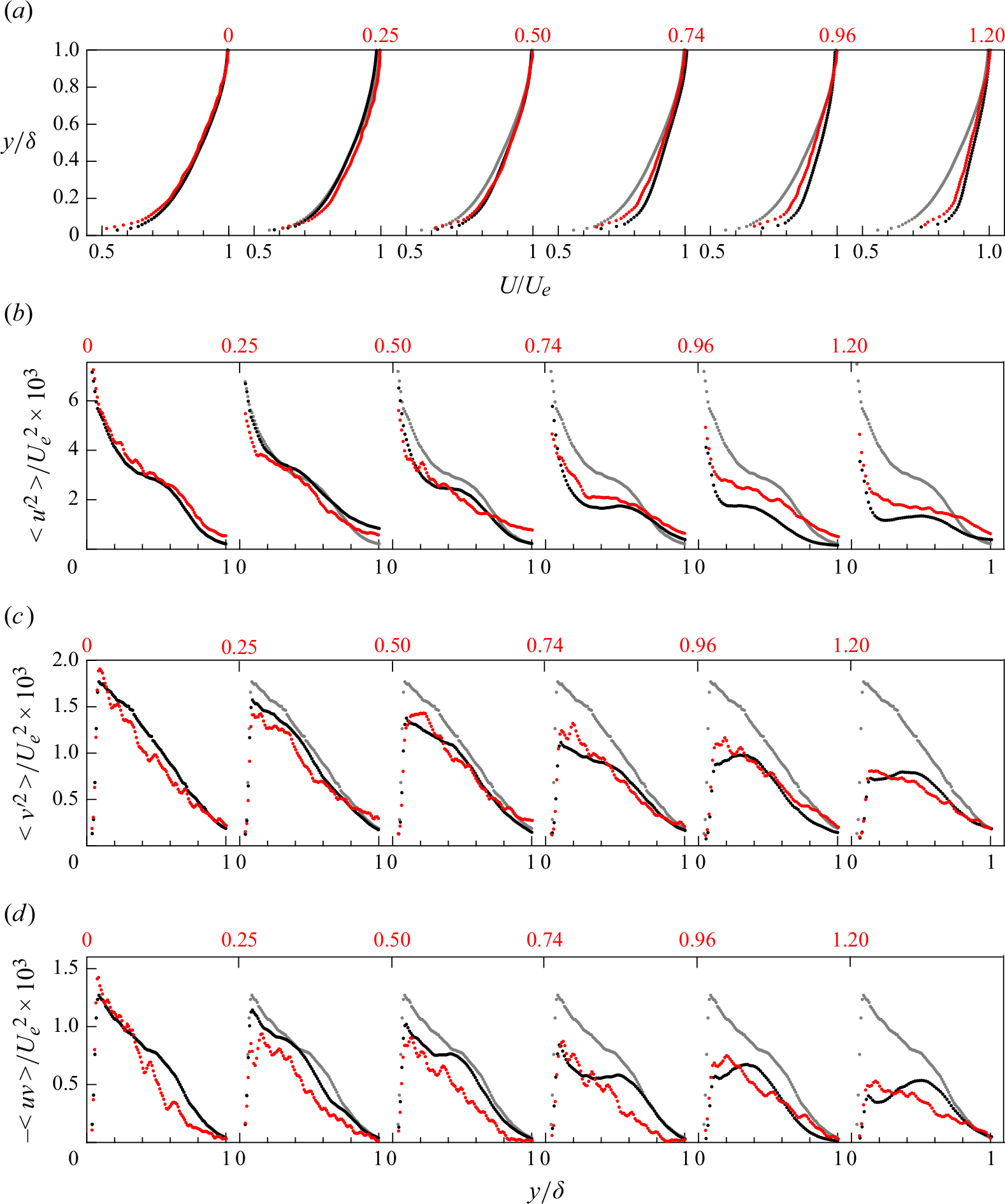
Ensemble-averaged unsteady, outer-scaled turbulent statistics at station $A$
at
$A$
at $\bar {K} = 0$
,
$\bar {K} = 0$
, $0.25$
,
$0.25$
, $0.5$
,
$0.5$
, $0.74$
,
$0.74$
, $0.96$
,
$0.96$
, $1.2$
. (a) Mean streamwise velocity profiles. (b) Streamwise Reynolds stress. (c) Wall-normal Reynolds stress. (d) Reynolds shear stress. Profiles at subsequent
$1.2$
. (a) Mean streamwise velocity profiles. (b) Streamwise Reynolds stress. (c) Wall-normal Reynolds stress. (d) Reynolds shear stress. Profiles at subsequent $\bar {K}$
are shifted by 0.5 units for (a) and 1.1 units for (b), (c) and (d) along the
$\bar {K}$
are shifted by 0.5 units for (a) and 1.1 units for (b), (c) and (d) along the $x$
-axis for visual clarity. Here (
$x$
-axis for visual clarity. Here (![]() ) ZPG, (
) ZPG, (![]() ) steady FAPG, (
) steady FAPG, (![]() ) unsteady FAPG.
) unsteady FAPG.
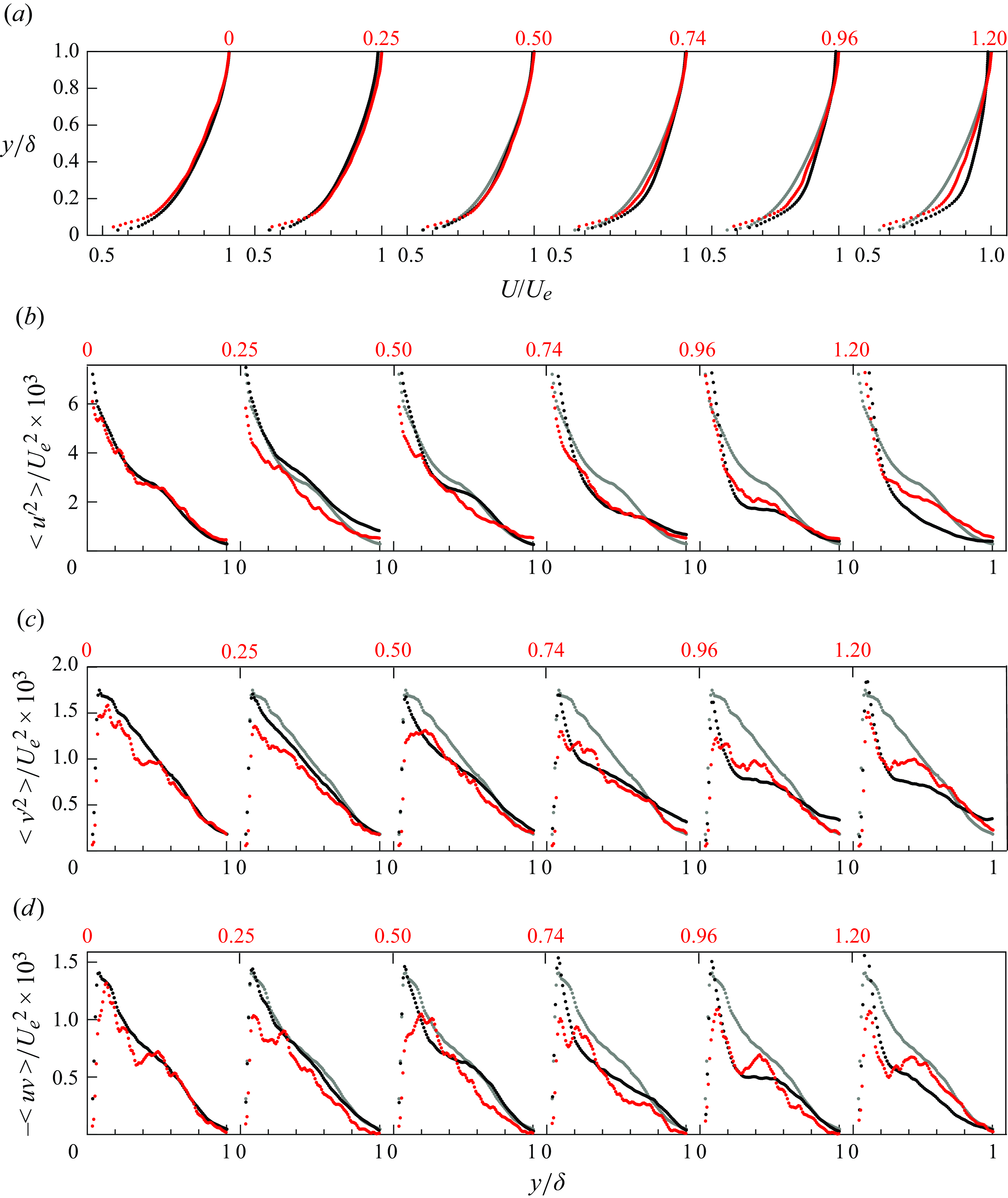
Ensemble-averaged unsteady, outer-scaled turbulent statistics at station $B$
at
$B$
at $\bar {K} = 0$
,
$\bar {K} = 0$
, $0.25$
,
$0.25$
, $0.5$
,
$0.5$
, $0.74$
,
$0.74$
, $0.96$
,
$0.96$
, $1.2$
. (a) Mean streamwise velocity profiles. (b) Streamwise Reynolds stress. (c) Wall-normal Reynolds stress. (d) Reynolds shear stress. Profiles at subsequent
$1.2$
. (a) Mean streamwise velocity profiles. (b) Streamwise Reynolds stress. (c) Wall-normal Reynolds stress. (d) Reynolds shear stress. Profiles at subsequent $\bar {K}$
are shifted by 0.5 units for (a) and 1.1 units for (b), (c) and (d) along the
$\bar {K}$
are shifted by 0.5 units for (a) and 1.1 units for (b), (c) and (d) along the $x$
-axis for visual clarity. Here (
$x$
-axis for visual clarity. Here (![]() ) ZPG, (
) ZPG, (![]() ) steady FAPG, (
) steady FAPG, (![]() ) unsteady FAPG.
) unsteady FAPG.
At $\bar {K}$
= 0, the steady and unsteady TBLs are at a ZPG condition. The corresponding statistical profiles collapse in figure 4 and figure 5 within the above-noted experimental uncertainties. As the pressure gradient is rapidly applied, the unsteady streamwise mean around the exit of the FPG region (figure 4
a) is seen to initially overshoot (
$\bar {K}$
= 0, the steady and unsteady TBLs are at a ZPG condition. The corresponding statistical profiles collapse in figure 4 and figure 5 within the above-noted experimental uncertainties. As the pressure gradient is rapidly applied, the unsteady streamwise mean around the exit of the FPG region (figure 4
a) is seen to initially overshoot ( $\bar {K}$
= 0.25) the corresponding steady-state profile, then undershoot it (
$\bar {K}$
= 0.25) the corresponding steady-state profile, then undershoot it ( $\bar {K}$
= 1), before starting to approach the steady-state mean towards the end of the transient (
$\bar {K}$
= 1), before starting to approach the steady-state mean towards the end of the transient ( $\bar {K}$
= 1.2). The comparison suggests a less accelerated TBL at the end of the transient compared with the corresponding steady pressure gradient imposition. Similar observations of overshoot, undershoot and recovery in the mean and second-order statistics have been noted in temporally accelerated pipe and channel flows (He & Jackson Reference He and Jackson2000; Mathur et al. Reference Mathur, Gorji, He, Seddighi, Vardy, O’Donoghue and Pokrajac2018). The initial stage is said to be dominated by inertial forces, resulting in large mean velocity gradients near the wall and a rapid increase in viscous shear stress, which later relaxes as the turbulence responds to the acceleration. Here, the sudden application of the FAPG causes the external flow upstream of station A to rapidly accelerate in time, in addition to the spatial acceleration, contributing to the initial over-response observed. The following under-response to the applied acceleration is counter-intuitive, however, and is subject to further inquiry in subsequent sections.
$\bar {K}$
= 1.2). The comparison suggests a less accelerated TBL at the end of the transient compared with the corresponding steady pressure gradient imposition. Similar observations of overshoot, undershoot and recovery in the mean and second-order statistics have been noted in temporally accelerated pipe and channel flows (He & Jackson Reference He and Jackson2000; Mathur et al. Reference Mathur, Gorji, He, Seddighi, Vardy, O’Donoghue and Pokrajac2018). The initial stage is said to be dominated by inertial forces, resulting in large mean velocity gradients near the wall and a rapid increase in viscous shear stress, which later relaxes as the turbulence responds to the acceleration. Here, the sudden application of the FAPG causes the external flow upstream of station A to rapidly accelerate in time, in addition to the spatial acceleration, contributing to the initial over-response observed. The following under-response to the applied acceleration is counter-intuitive, however, and is subject to further inquiry in subsequent sections.
The unsteady Reynolds stresses in figure 4(b–d) show certain features of the corresponding steady-states discussed in § 3.1.1. These include the suppression of stresses with increasing $\bar {K}$
, consistent with an accelerated TBL, and the formation and evolution of a ‘knee point’ (i.e. the valley point of the two-peak structure) in the u-RS, suggesting the existence of an internal layer in the unsteady flow. But the profiles do not exhibit quasisteady behaviour. The u-RS follows a temporal evolution similar to the streamwise mean, initially over-responding to the unsteady acceleration compared with the corresponding steady-state (
$\bar {K}$
, consistent with an accelerated TBL, and the formation and evolution of a ‘knee point’ (i.e. the valley point of the two-peak structure) in the u-RS, suggesting the existence of an internal layer in the unsteady flow. But the profiles do not exhibit quasisteady behaviour. The u-RS follows a temporal evolution similar to the streamwise mean, initially over-responding to the unsteady acceleration compared with the corresponding steady-state ( $\bar {K} \leqslant 0.25$
), then under-responding (
$\bar {K} \leqslant 0.25$
), then under-responding ( $0.25 \lt \bar {K} \lt 0.96$
) and finally tending towards the steady-state response (
$0.25 \lt \bar {K} \lt 0.96$
) and finally tending towards the steady-state response ( $\bar {K} = 1$
). At
$\bar {K} = 1$
). At $\bar {K}$
= 1.2, the scaled u-RS is higher in magnitude for the unsteady case, as if the unsteady TBL has experienced a weaker acceleration compared with the steady TBL. Along with the overshooting exhibited by the unsteady u-RS at
$\bar {K}$
= 1.2, the scaled u-RS is higher in magnitude for the unsteady case, as if the unsteady TBL has experienced a weaker acceleration compared with the steady TBL. Along with the overshooting exhibited by the unsteady u-RS at $\bar {K}$
= 0.25, a knee point appears to form at
$\bar {K}$
= 0.25, a knee point appears to form at $y = 0.2 \delta$
, whereas the steady profile has not developed a clear knee point at this
$y = 0.2 \delta$
, whereas the steady profile has not developed a clear knee point at this $\bar {K}$
. The unsteady knee point was consistently observed at nearby locations beyond experimental uncertainty. In the v-RS and uv-RS shown in figure 4(c,d), the flow evolution appears to have resulted in the formation of a single-peak structure, rather than the two-peak structure seen in the steady profiles. Note that, as seen in figure 5, the unsteady statistics are able to represent distinct peaks, if they did exist.
$\bar {K}$
. The unsteady knee point was consistently observed at nearby locations beyond experimental uncertainty. In the v-RS and uv-RS shown in figure 4(c,d), the flow evolution appears to have resulted in the formation of a single-peak structure, rather than the two-peak structure seen in the steady profiles. Note that, as seen in figure 5, the unsteady statistics are able to represent distinct peaks, if they did exist.
Around station $B$
(figure 5), the unsteady flow is spatially decelerated but is temporally accelerating. The steady states also vary correspondingly, i.e. the stronger pressure gradients are associated with a more accelerated external flow. The unsteady mean profile in figure 5(a) exhibits a slight overshoot in
$B$
(figure 5), the unsteady flow is spatially decelerated but is temporally accelerating. The steady states also vary correspondingly, i.e. the stronger pressure gradients are associated with a more accelerated external flow. The unsteady mean profile in figure 5(a) exhibits a slight overshoot in $y\lt 0.2\delta$
at
$y\lt 0.2\delta$
at $\bar {K}=0.25$
compared with the corresponding steady-state mean. This could be a residual of the initial over-acceleration seen around station
$\bar {K}=0.25$
compared with the corresponding steady-state mean. This could be a residual of the initial over-acceleration seen around station $A$
. For the second half of unsteady time (
$A$
. For the second half of unsteady time ( $\bar {K}\gt 0.5$
), the unsteady means show a stronger response to the APG (or stronger spatial deceleration from station
$\bar {K}\gt 0.5$
), the unsteady means show a stronger response to the APG (or stronger spatial deceleration from station $A$
to
$A$
to $B$
), while the corresponding steady states remain significantly fuller. The steady APG mean behaviour, as summarised in § 3.1.1, is a result of the upstream FPG also being stronger for higher
$B$
), while the corresponding steady states remain significantly fuller. The steady APG mean behaviour, as summarised in § 3.1.1, is a result of the upstream FPG also being stronger for higher $\bar {K}$
, which builds a stronger resistance in the TBL to the APG. In the unsteady case, however, the mean develops a velocity deficit compared with the ZPG case near the wall in
$\bar {K}$
, which builds a stronger resistance in the TBL to the APG. In the unsteady case, however, the mean develops a velocity deficit compared with the ZPG case near the wall in $\bar {K} \gt 0.52$
. This may indicate that the upstream FPG’s influence could be weaker in the unsteady case.
$\bar {K} \gt 0.52$
. This may indicate that the upstream FPG’s influence could be weaker in the unsteady case.
As in the response around station $A$
(figure 4), the temporal evolution of the u-RS around station
$A$
(figure 4), the temporal evolution of the u-RS around station $B$
is similar to that of the mean at that location. The unsteady u-RS initially overshoots the suppression of the steady u-RS at
$B$
is similar to that of the mean at that location. The unsteady u-RS initially overshoots the suppression of the steady u-RS at $\bar {K} = 0.25$
, and after
$\bar {K} = 0.25$
, and after $\bar {K}$
= 0.5, the wake region stresses in
$\bar {K}$
= 0.5, the wake region stresses in $y \gt 0.2\delta$
are seen to recover rather than get further suppressed as they do in the corresponding steady u-RS. Similar recovery of stresses as the APG strengthens with
$y \gt 0.2\delta$
are seen to recover rather than get further suppressed as they do in the corresponding steady u-RS. Similar recovery of stresses as the APG strengthens with $\bar {K}$
is seen in the v-RS and uv-RS in
$\bar {K}$
is seen in the v-RS and uv-RS in $\bar {K} \gt$
0.5, in the region
$\bar {K} \gt$
0.5, in the region $y\gt 0.2 \delta$
. Such a recovery of stresses and the formation of an outer peak is striking as it is more characteristic of an APG TBL without an upstream FPG (or internal layer). There is also a difference between the steady and unsteady cases in terms of the magnitude of the first peaks of the v-RS and uv-RS. It was discussed earlier in § 3.1.1 that the first peak of the steady stress profiles strengthened in
$y\gt 0.2 \delta$
. Such a recovery of stresses and the formation of an outer peak is striking as it is more characteristic of an APG TBL without an upstream FPG (or internal layer). There is also a difference between the steady and unsteady cases in terms of the magnitude of the first peaks of the v-RS and uv-RS. It was discussed earlier in § 3.1.1 that the first peak of the steady stress profiles strengthened in $x$
due to the growth of the internal layer. As the boundary layer reaches station
$x$
due to the growth of the internal layer. As the boundary layer reaches station $B$
, at
$B$
, at $\bar {K}$
= 1.2, the first peaks of the v-RS and uv-RS are seen in figure 5(c,d) to be 26
$\bar {K}$
= 1.2, the first peaks of the v-RS and uv-RS are seen in figure 5(c,d) to be 26 $\, \%$
and 33
$\, \%$
and 33 $\, \%$
lower in the unsteady case than the corresponding peaks of the steady-states. This again suggests that, in the unsteady case, the FPG’s influence is weaker than for the equivalent steady case.
$\, \%$
lower in the unsteady case than the corresponding peaks of the steady-states. This again suggests that, in the unsteady case, the FPG’s influence is weaker than for the equivalent steady case.
3.2. Vortex organisation
Under the influence of the steady FAPGs, the mean spanwise vorticity field exhibited strong changes from canonical behaviour, as discussed in Parthasarathy & Saxton-Fox (Reference Parthasarathy and Saxton-Fox2023). A two-layer structure was observed, showcasing the internal layer as a region of strong spanwise vorticity, and the outer layer as a relatively passive region, consistent with the picture suggested by the Reynolds stresses. This vorticity bifurcation was shown to be the result of a significant rearrangement of vortices and their strength caused by the applied FAPG and the subsequent formation of the internal layer.
In the unsteady case, the statistics show partial signatures of the internal layer via the appearance of a knee point in the u-RS, but it is not conclusive whether an internal layer is present and if it is, its dominance in the flow. To clarify this and to better understand the effect of unsteadiness on the organisation of the boundary layer, the strength of vortices and the mean population of vortices are studied in $y$
and in time. The swirling strength criterion (or
$y$
and in time. The swirling strength criterion (or $\lambda _{ci}$
- method) is chosen. Since the direction of rotation is not embedded in
$\lambda _{ci}$
- method) is chosen. Since the direction of rotation is not embedded in $\lambda _{ci}$
, it is conventional to define
$\lambda _{ci}$
, it is conventional to define $\Lambda _{ci}$ $\equiv$ $\lambda _{ci} \times {\omega _z}/{|\omega _z|}$
, assigning the direction of instantaneous vorticity to the swirling strength. The r.m.s. of this swirling strength parameter (
$\lambda _{ci} \times {\omega _z}/{|\omega _z|}$
, assigning the direction of instantaneous vorticity to the swirling strength. The r.m.s. of this swirling strength parameter ( $\Lambda ^{RMS}_{ci}$
) represents the characteristic magnitude of
$\Lambda ^{RMS}_{ci}$
) represents the characteristic magnitude of $\Lambda _{ci}$
at a given location and is used in the definition of a universal threshold for vortex detection, given by
$\Lambda _{ci}$
at a given location and is used in the definition of a universal threshold for vortex detection, given by ${\Lambda _{ci}}/{\Lambda ^{RMS}_{ci}} \geqslant 1.5$
(Wu & Christensen Reference Wu and Christensen2006; Chen et al. Reference Chen, Zhong, Qi and Wang2015). Only vortices larger than
${\Lambda _{ci}}/{\Lambda ^{RMS}_{ci}} \geqslant 1.5$
(Wu & Christensen Reference Wu and Christensen2006; Chen et al. Reference Chen, Zhong, Qi and Wang2015). Only vortices larger than $3\Delta l^+ (= 26.7)$
are included, effectively applying a spatial filter that excludes vortices smaller than three grid points in both the streamwise and wall-normal directions. Prograde and retrograde vortices are counted separately. Here
$3\Delta l^+ (= 26.7)$
are included, effectively applying a spatial filter that excludes vortices smaller than three grid points in both the streamwise and wall-normal directions. Prograde and retrograde vortices are counted separately. Here $\Lambda ^{RMS}_{ci}$
is also studied on its own as it is a statistical estimate of the strength of vortices in the flow.
$\Lambda ^{RMS}_{ci}$
is also studied on its own as it is a statistical estimate of the strength of vortices in the flow.
Variations in the strength of vortices with wall-normal height from the flat wall for the unsteady (solid lines) and steady (dashed lines) boundary layers at the following matched FAPG magnitudes: (a) $\bar {K} = 0$
, (b)
$\bar {K} = 0$
, (b) $\bar {K}$
= 0.74 and (c)
$\bar {K}$
= 0.74 and (c) $\bar {K}$
= 1.2.
$\bar {K}$
= 1.2.
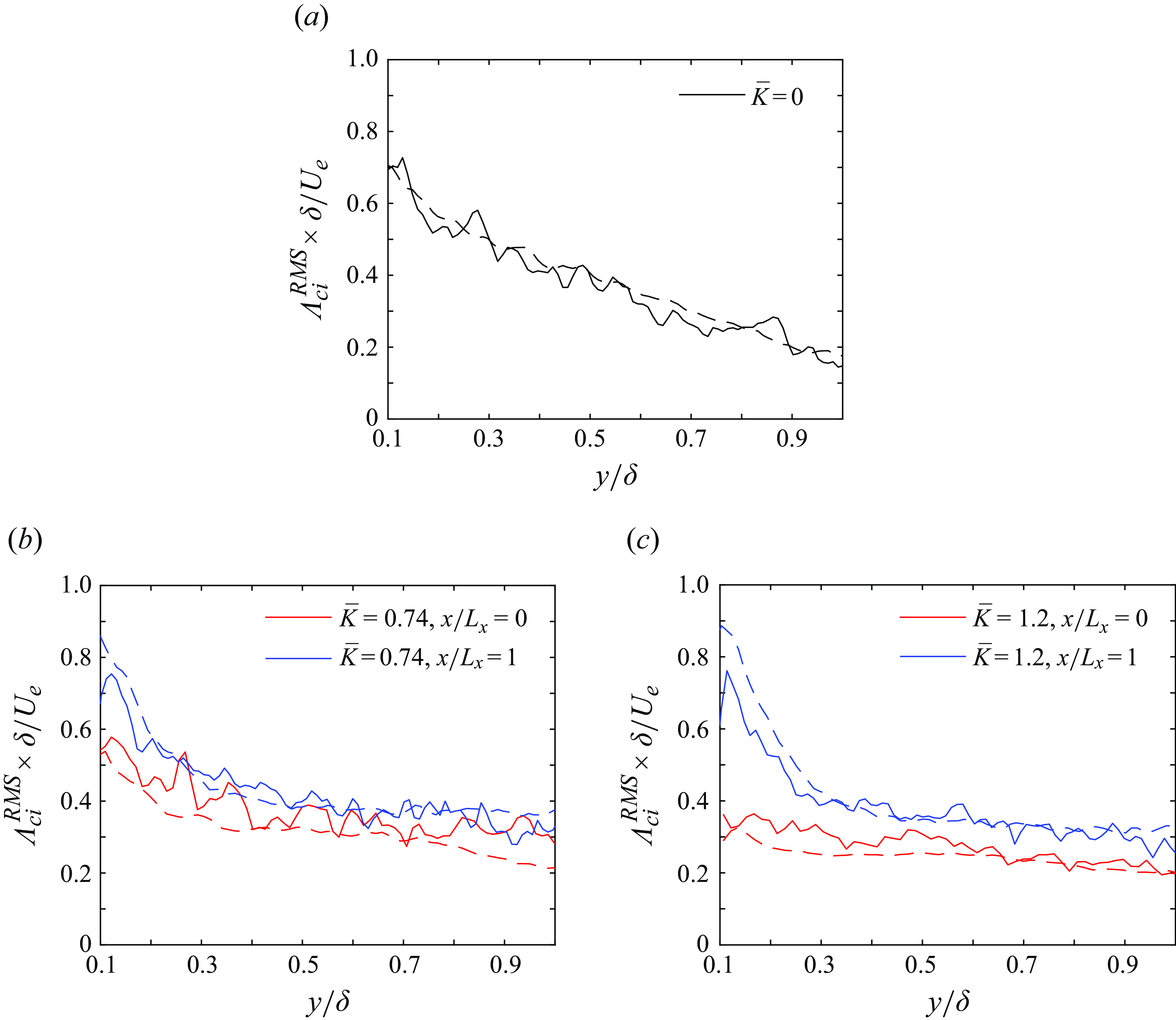
The results are presented at discrete time instances by comparing them with the corresponding steady pressure gradient profiles, as in the case of the mean and Reynolds stresses. Local outer-scaled $\Lambda _{ci}^{RMS}$
is plotted with wall-normal distance from the flat wall in figure 6 at three time instances: at the start of the unsteady time when the TBL is under a ZPG (
$\Lambda _{ci}^{RMS}$
is plotted with wall-normal distance from the flat wall in figure 6 at three time instances: at the start of the unsteady time when the TBL is under a ZPG ( $\bar {K} = 0$
, figure 6
a); an instance during the pressure gradient imposition when the FAPG is moderate (
$\bar {K} = 0$
, figure 6
a); an instance during the pressure gradient imposition when the FAPG is moderate ( $\bar {K} = 0.74$
, figure 6
b); at the end of unsteady time when the FAPG is strong (
$\bar {K} = 0.74$
, figure 6
b); at the end of unsteady time when the FAPG is strong ( $\bar {K}$
= 1.2, figure 6
c). In figure 6(b,c), the profiles are shown at stations
$\bar {K}$
= 1.2, figure 6
c). In figure 6(b,c), the profiles are shown at stations $A$
,
$A$
, $x/L_x =0$
and
$x/L_x =0$
and $B$
,
$B$
, $x/L_x =1$
to observe the overall spatial variation. The solid lines correspond to the unsteady flow and the dashed lines to the matched steady-state flow. Figure 6(a) demonstrates the equivalence of the steady and unsteady flows at the ZPG instance, despite the noisier unsteady result.
$x/L_x =1$
to observe the overall spatial variation. The solid lines correspond to the unsteady flow and the dashed lines to the matched steady-state flow. Figure 6(a) demonstrates the equivalence of the steady and unsteady flows at the ZPG instance, despite the noisier unsteady result.
Increasing the strength of the FAPG in time was seen to cause an organisation of the vortices similar to the corresponding steady FAPGs in a few ways, but with some important differences. The strength of vortices at station $A$
,
$A$
, $x/L_x = 0$
, consistently decreased in time due to the increasing upstream FPG, and at a given instance, as the flow progressed through the local APG and reached station
$x/L_x = 0$
, consistently decreased in time due to the increasing upstream FPG, and at a given instance, as the flow progressed through the local APG and reached station $B$
, the vortices strengthened. A peak in
$B$
, the vortices strengthened. A peak in $y \lt 0.3\delta$
, associated with the internal layer in the steady cases (Parthasarathy & Saxton-Fox Reference Parthasarathy and Saxton-Fox2023), was observed in the unsteady case as well, present but small at station
$y \lt 0.3\delta$
, associated with the internal layer in the steady cases (Parthasarathy & Saxton-Fox Reference Parthasarathy and Saxton-Fox2023), was observed in the unsteady case as well, present but small at station $A$
and clearly visible at station
$A$
and clearly visible at station $B$
. But the magnitudes of scaled
$B$
. But the magnitudes of scaled $\lambda _{ci}^{RMS}$
are higher than the equivalent steady FAPG TBL at station
$\lambda _{ci}^{RMS}$
are higher than the equivalent steady FAPG TBL at station $A$
. The magnitude of the peak can also be seen to be lower at station
$A$
. The magnitude of the peak can also be seen to be lower at station $B$
than the steady case, while the magnitude outside the internal layer matches the corresponding steady flow at station
$B$
than the steady case, while the magnitude outside the internal layer matches the corresponding steady flow at station $B$
up to
$B$
up to $y = 0.8\delta$
. The wall-normal location of the peak, too, can be observed to be farther away from the wall in the unsteady case. These observations were found to be consistent at all times investigated.
$y = 0.8\delta$
. The wall-normal location of the peak, too, can be observed to be farther away from the wall in the unsteady case. These observations were found to be consistent at all times investigated.
Mean population of vortices with wall-normal height in the unsteady (solid lines) and steady (dashed lines) boundary layers at the following matched FAPG magnitudes: (a) $\bar {K} = 0$
, (b,c)
$\bar {K} = 0$
, (b,c) $\bar {K}$
= 0.74 and (d,e)
$\bar {K}$
= 0.74 and (d,e) $\bar {K}$
= 1.2. Panels (b,d) are at
$\bar {K}$
= 1.2. Panels (b,d) are at $x/L_x$
= 0 and (c,e) are at
$x/L_x$
= 0 and (c,e) are at $x/L_x$
= 1.
$x/L_x$
= 1.
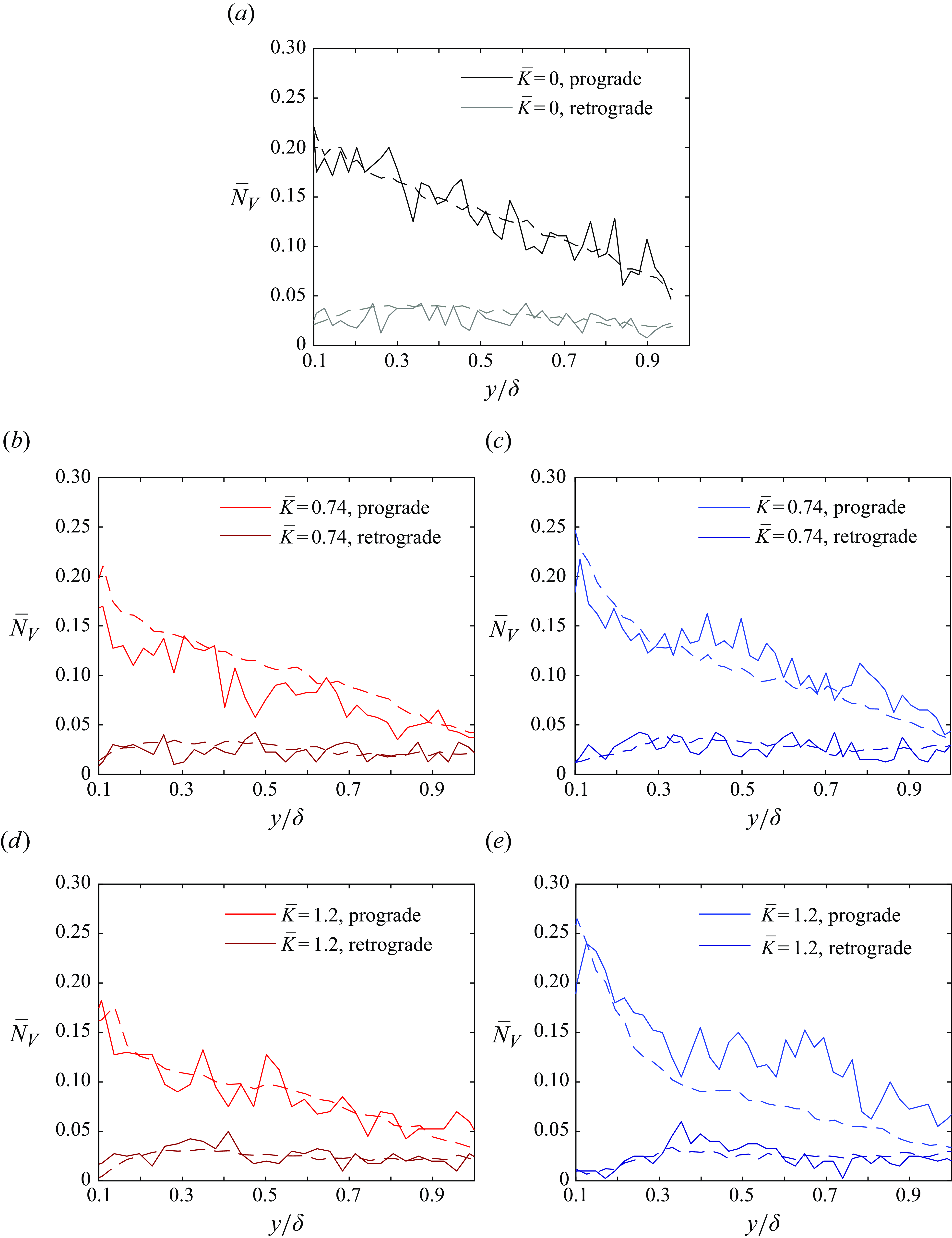
The vortex population trends in the boundary layer showed that prograde vortices exhibited some differences between the unsteady and steady FAPGs, whereas retrograde vortices remained quasisteady. These are demonstrated at the same three times considered in figure 6: when $\bar {K}$
= 0 (figure 7
a);
$\bar {K}$
= 0 (figure 7
a); $\bar {K} = 0.74$
(figure 7
b,c);
$\bar {K} = 0.74$
(figure 7
b,c); $\bar {K} = 1.2$
(figure 7
d,e). Figure 7(b,d) show results at station
$\bar {K} = 1.2$
(figure 7
d,e). Figure 7(b,d) show results at station $A$
and figure 7(c,e) at station
$A$
and figure 7(c,e) at station $B$
, for clarity in presentation. Focusing on the prograde vortices (red and blue solid and dashed lines in figure 7
b–e): for a significant portion of unsteady time (
$B$
, for clarity in presentation. Focusing on the prograde vortices (red and blue solid and dashed lines in figure 7
b–e): for a significant portion of unsteady time ( $\bar {K} \lt 0.9$
), the mean population is found to stay lower than the corresponding steady case at station
$\bar {K} \lt 0.9$
), the mean population is found to stay lower than the corresponding steady case at station $A$
(which stays relatively unchanged from the population under ZPG). At station
$A$
(which stays relatively unchanged from the population under ZPG). At station $B$
, not only does the mean population increase within the internal layer as expected, but also in the outer layer. The increase is more significant at later times (or under strong FAPG). Similar to the wall-normal profiles of
$B$
, not only does the mean population increase within the internal layer as expected, but also in the outer layer. The increase is more significant at later times (or under strong FAPG). Similar to the wall-normal profiles of $\Lambda _{ci}^{RMS}$
, the peak in the vortex population is observed to be slightly farther away from the wall than the corresponding steady cases. It was previously observed in the steady cases that the retrograde vortices exhibited minimal changes with
$\Lambda _{ci}^{RMS}$
, the peak in the vortex population is observed to be slightly farther away from the wall than the corresponding steady cases. It was previously observed in the steady cases that the retrograde vortices exhibited minimal changes with $\bar {K}$
and
$\bar {K}$
and $x$
except for a decrease within the internal layer with
$x$
except for a decrease within the internal layer with $x$
. The same variations are seen in the unsteady cases, suggesting that the retrograde vortices are relatively unaffected by the imposed unsteadiness.
$x$
. The same variations are seen in the unsteady cases, suggesting that the retrograde vortices are relatively unaffected by the imposed unsteadiness.
Overall, the unsteadiness appears to have a complex effect on the vortex strength and population in this FAPG flow. At station $A$
, located at the exit of the FPG region, the vortices remain stronger than the corresponding steady-state flow throughout the unsteady time, but their population is lower in the unsteady case. The former could suggest that the unsteady flow did not realise the upstream FPG effect as much (as also suggested by the statistics), but the reduced population of vortices in parallel is counter-intuitive. The features observed were found to smoothly evolve in
$A$
, located at the exit of the FPG region, the vortices remain stronger than the corresponding steady-state flow throughout the unsteady time, but their population is lower in the unsteady case. The former could suggest that the unsteady flow did not realise the upstream FPG effect as much (as also suggested by the statistics), but the reduced population of vortices in parallel is counter-intuitive. The features observed were found to smoothly evolve in $x$
from stations
$x$
from stations $A$
to
$A$
to $B$
. At station
$B$
. At station $B$
, the strength and population of vortices have both clearly increased within
$B$
, the strength and population of vortices have both clearly increased within $y\lt 0.3\delta$
in a similar manner as the steady FAPGs, but the increase is consistently weaker in the unsteady case. This suggests that the internal layer does exist, but its growth is weaker in the unsteady case, which could either be due to the formation of a weaker layer or due to the temporal acceleration working against its growth in the APG region. Interestingly, a significant increase in the population of vortices is observed in the outer layer in the unsteady case, creating an outer peak that could be related to the outer peak observed in the second-order statistics at this station (figure 5
b–d). As mentioned earlier, this outer peak is more typical of ZAPG rather than FAPG TBLs. Here ZAPG is a zero-APG where the APG is preceded by a ZPG, defined to differentiate this from the FAPG studied.
$y\lt 0.3\delta$
in a similar manner as the steady FAPGs, but the increase is consistently weaker in the unsteady case. This suggests that the internal layer does exist, but its growth is weaker in the unsteady case, which could either be due to the formation of a weaker layer or due to the temporal acceleration working against its growth in the APG region. Interestingly, a significant increase in the population of vortices is observed in the outer layer in the unsteady case, creating an outer peak that could be related to the outer peak observed in the second-order statistics at this station (figure 5
b–d). As mentioned earlier, this outer peak is more typical of ZAPG rather than FAPG TBLs. Here ZAPG is a zero-APG where the APG is preceded by a ZPG, defined to differentiate this from the FAPG studied.
3.3. Turbulent energy spectrum
3.3.1. Steady FAPGs
A spectral decomposition of the flow under the steady FAPGs, discussed in-detail in Parthasarathy & Saxton-Fox (Reference Parthasarathy and Saxton-Fox2023), showed the power spectral densities (PSDs) of the streamwise velocity fluctuations at the exit of the FPG region to be suppressed everywhere, but more significantly in the outer layer, and shifted to longer wavelengths compared with the ZPG flow. The PSDs of the wall-normal fluctuations also exhibited strongly suppressed states, but the suppression was more uniform throughout the boundary layer. For the strongest pressure gradient considered, the spectral densities of large scales ( $\lambda _x = 3-5\delta$
) in the outer region in both the streamwise and wall-normal velocity spectra were reduced by almost an order of magnitude due to the upstream FPG. Within the APG, the PSD recovered. Most of the recovery happened within the internal layer, revealing the streamwise spectral composition of the internal layer to be of energetic large-scale structures (
$\lambda _x = 3-5\delta$
) in the outer region in both the streamwise and wall-normal velocity spectra were reduced by almost an order of magnitude due to the upstream FPG. Within the APG, the PSD recovered. Most of the recovery happened within the internal layer, revealing the streamwise spectral composition of the internal layer to be of energetic large-scale structures ( $\lambda _x = 3-8\delta$
) and relatively energetic smaller scales with
$\lambda _x = 3-8\delta$
) and relatively energetic smaller scales with $\lambda _x = 0.5-1.5\delta$
. The wall-normal velocity spectrum revealed energetic structures that are less streamwise elongated, in the range
$\lambda _x = 0.5-1.5\delta$
. The wall-normal velocity spectrum revealed energetic structures that are less streamwise elongated, in the range $0.1\delta \lt \lambda _x\lt 1\delta$
, clearly contained by the local internal layer edge.
$0.1\delta \lt \lambda _x\lt 1\delta$
, clearly contained by the local internal layer edge.
3.3.2. Unsteady FAPGs
Since the flow of interest is non-stationary, a Fourier decomposition is inappropriate. Time–frequency techniques that retain both frequency content and temporal information need to be used. Hence, the temporally varying power spectra of the TBL under the unsteady FAPG imposition are studied by computing the wavelet power spectra (WPS) of the temporally varying data. As before, the effects of unsteadiness on the spectral content of the TBL will be isolated from the effects of the spatial pressure gradients by making suitable comparisons with the steady spectra at matched FAPGs. The spectra will be presented in the premultiplied form, premultiplied by the streamwise wavenumber.
Comparison of the ZPG Fourier PSD and time-averaged wavelet PSD at wall-normal location: (a) $y = 0.06 \delta$
and (b)
$y = 0.06 \delta$
and (b) $y = 0.4 \delta$
.
$y = 0.4 \delta$
.
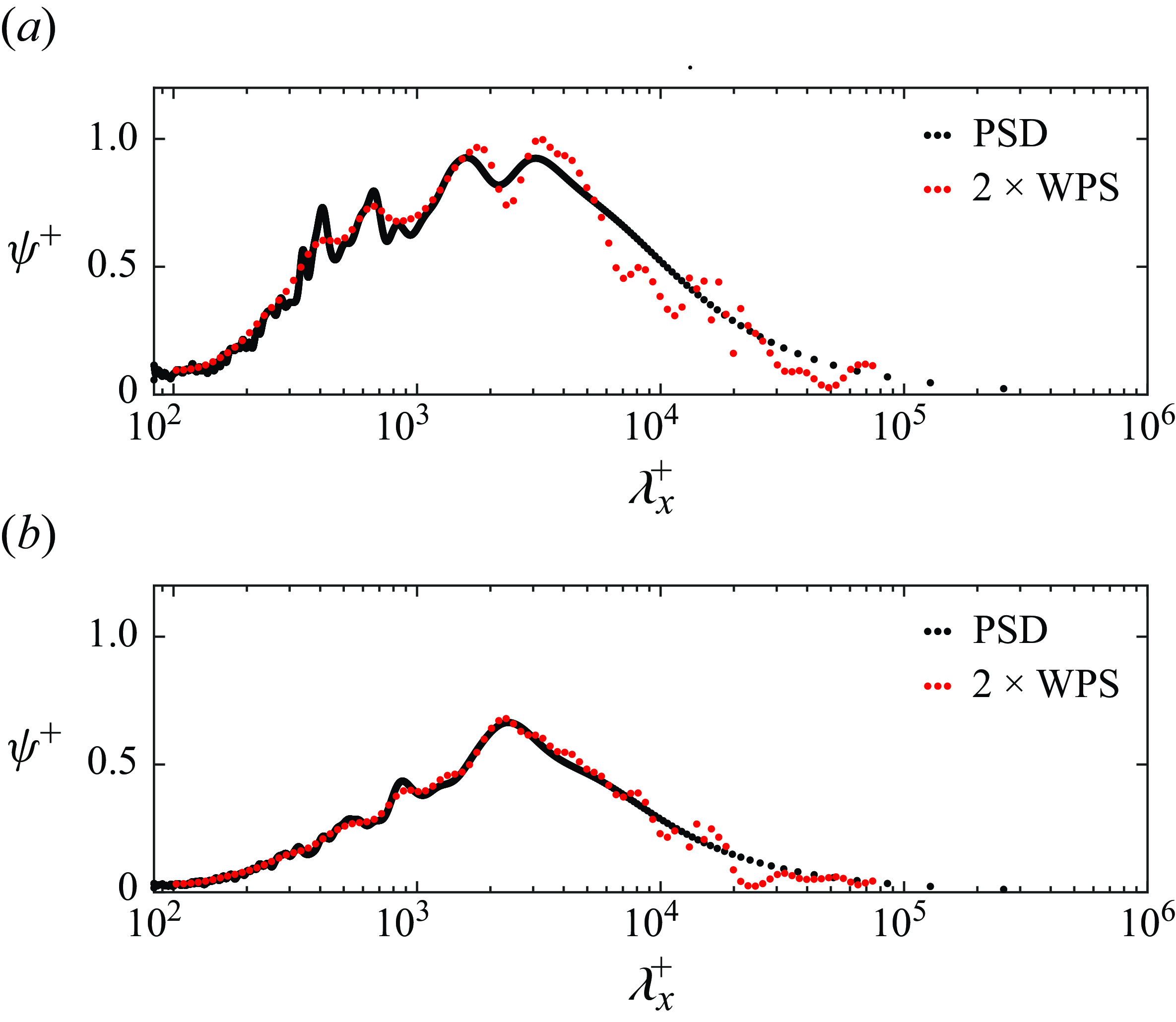
The WPS is obtained by computing the continuous wavelet transform (CWT) of every ensemble using the analytic Morse wavelet, with a shape parameter ( $\gamma$
) of 3 and oscillation control parameter (
$\gamma$
) of 3 and oscillation control parameter ( $\beta _1$
) of 20. The WPS are then averaged across the 400 unsteady ensembles and normalised to get spatiotemporally varying wavelet coefficients. To avoid edge effects in the cone of influence, data recorded just before and after the transient were also used in computing the CWT, which were then cropped out to keep the WPS during the transient alone. For each of the steady cases, the CWT is applied after splitting the 6170 time-correlated steady fields into 17 ensembles, so as to get the same frequency resolution as the unsteady case. The WPS are then averaged across the 17 ensembles and averaged in time to get normalised wavelet coefficients that only vary along the spatial coordinates. The focus of this analysis is on the WPS at two spatial locations, station
$\beta _1$
) of 20. The WPS are then averaged across the 400 unsteady ensembles and normalised to get spatiotemporally varying wavelet coefficients. To avoid edge effects in the cone of influence, data recorded just before and after the transient were also used in computing the CWT, which were then cropped out to keep the WPS during the transient alone. For each of the steady cases, the CWT is applied after splitting the 6170 time-correlated steady fields into 17 ensembles, so as to get the same frequency resolution as the unsteady case. The WPS are then averaged across the 17 ensembles and averaged in time to get normalised wavelet coefficients that only vary along the spatial coordinates. The focus of this analysis is on the WPS at two spatial locations, station $A$
and station
$A$
and station $B$
, and two wall-normal locations,
$B$
, and two wall-normal locations, $y = 0.06 \delta$
and
$y = 0.06 \delta$
and $y=0.4\delta$
. Station
$y=0.4\delta$
. Station $A$
captures the effect of the upstream FPG and station
$A$
captures the effect of the upstream FPG and station $B$
captures the effect of the APG cumulated over the effect of the upstream FPG. Here
$B$
captures the effect of the APG cumulated over the effect of the upstream FPG. Here $y = 0.06 \delta$
is located within the energetic region associated with the internal layer in the steady case, and
$y = 0.06 \delta$
is located within the energetic region associated with the internal layer in the steady case, and $y = 0.4 \delta$
is a representative outer region location where large scales are expected to be dominant in the ZPG PSD (Parthasarathy & Saxton-Fox Reference Parthasarathy and Saxton-Fox2023).
$y = 0.4 \delta$
is a representative outer region location where large scales are expected to be dominant in the ZPG PSD (Parthasarathy & Saxton-Fox Reference Parthasarathy and Saxton-Fox2023).
To validate the computation of the WPS, the time-averaged WPS from the ZPG case ( $\bar {K}$
= 0) is compared with the PSD of the same data. The comparison is shown in figure 8 at the two wall-normal locations at the focus of this section. Inner-scaling is chosen due to the availability of
$\bar {K}$
= 0) is compared with the PSD of the same data. The comparison is shown in figure 8 at the two wall-normal locations at the focus of this section. Inner-scaling is chosen due to the availability of $u_\tau$
for the ZPG condition and for ease of comparison with the literature, such as the PSDs shown in Harun et al. (Reference Harun, Monty and Marusic2011) at similar wall-normal heights. The WPS and PSD computations match well, with the WPS resolving long wavelengths (
$u_\tau$
for the ZPG condition and for ease of comparison with the literature, such as the PSDs shown in Harun et al. (Reference Harun, Monty and Marusic2011) at similar wall-normal heights. The WPS and PSD computations match well, with the WPS resolving long wavelengths ( $\lambda _x^+ \gt 4000$
) better. The WPS was found to be half the magnitude of the PSD, which is similar to the factor of two difference reported by Severino et al. (Reference Severino, Silvestri, Ghanadi, Cazzolato and Arjomandi2020) between their WPS and PSD.
$\lambda _x^+ \gt 4000$
) better. The WPS was found to be half the magnitude of the PSD, which is similar to the factor of two difference reported by Severino et al. (Reference Severino, Silvestri, Ghanadi, Cazzolato and Arjomandi2020) between their WPS and PSD.
The contour plots in figure 9 show the time-varying WPS for the unsteady TBL as the pressure gradient is dynamically imposed, at station $A$
in figure 9(a,c) and at station
$A$
in figure 9(a,c) and at station $B$
in figure 9(b,d). Figure 9(a,b) are at
$B$
in figure 9(b,d). Figure 9(a,b) are at $y = 0.4 \delta$
and figure 9(c,d) are at
$y = 0.4 \delta$
and figure 9(c,d) are at $y = 0.06\delta$
. In each, the time-averaged WPS from the steady pressure gradient cases with
$y = 0.06\delta$
. In each, the time-averaged WPS from the steady pressure gradient cases with $\bar {K} = 0$
and
$\bar {K} = 0$
and $\bar {K} = 1.2$
, corresponding to the steady ZPG and strongest FAPG cases, are shown as black line plots cast at the respective
$\bar {K} = 1.2$
, corresponding to the steady ZPG and strongest FAPG cases, are shown as black line plots cast at the respective $\bar {K}$
values. Wavenumbers obtained from the WPS computation have been converted to wavelengths using the local edge velocity in space and time and scaled with the corresponding local boundary layer thickness.
$\bar {K}$
values. Wavenumbers obtained from the WPS computation have been converted to wavelengths using the local edge velocity in space and time and scaled with the corresponding local boundary layer thickness.
Wavelet power spectrum of the flat-plate TBL during UPG imposition at (a) station $A$
at
$A$
at $y = 0.4\delta$
, (b) station
$y = 0.4\delta$
, (b) station $B$
at
$B$
at $y = 0.4\delta$
, (c) station
$y = 0.4\delta$
, (c) station $A$
at
$A$
at $y = 0.06\delta$
and (d) station
$y = 0.06\delta$
and (d) station $B$
at
$B$
at $y = 0.06\delta$
. The line plots in each figure at
$y = 0.06\delta$
. The line plots in each figure at $\bar {K}$
= 0 and
$\bar {K}$
= 0 and $\bar {K}$
= 1.2 show the time-averaged WPS of the steady cases with
$\bar {K}$
= 1.2 show the time-averaged WPS of the steady cases with $\bar {K}$
= 0 and
$\bar {K}$
= 0 and $\bar {K}$
= 1.2 at the respective spatial locations.
$\bar {K}$
= 1.2 at the respective spatial locations.
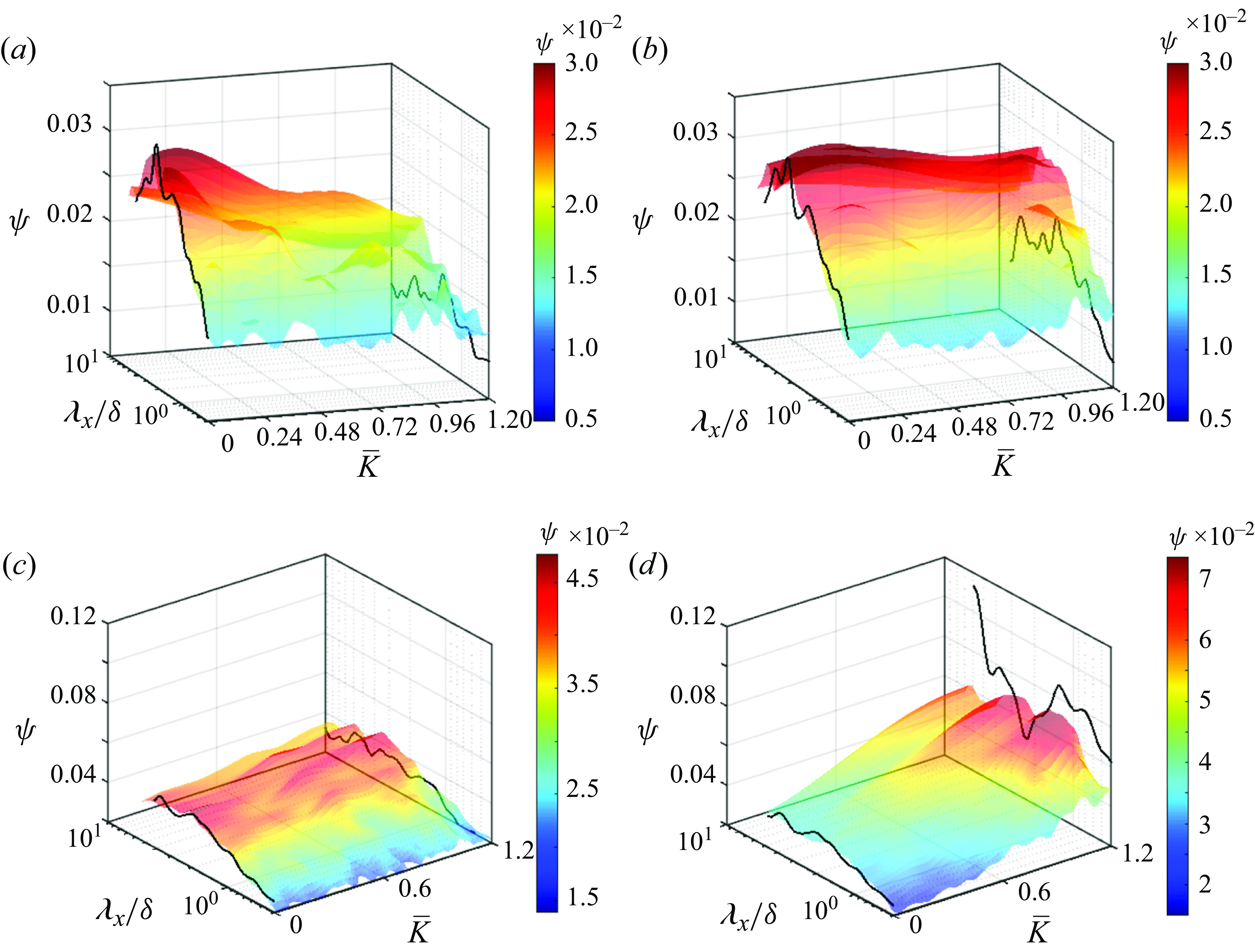
At the four locations shown in figure 9(a–d), the steady and unsteady spectra at $\bar {K}$
= 0 (contour levels for the unsteady case and line plots for the steady case) are seen to agree well, which further validates the comparison of WPS between the steady and unsteady cases at matched
$\bar {K}$
= 0 (contour levels for the unsteady case and line plots for the steady case) are seen to agree well, which further validates the comparison of WPS between the steady and unsteady cases at matched $\bar {K}$
. The spectra at
$\bar {K}$
. The spectra at $y = 0.4\delta$
(figure 9
a,b) are considered first. At station
$y = 0.4\delta$
(figure 9
a,b) are considered first. At station $A$
(figure 9
a), the unsteady WPS shows a strong reduction of energy contained in all scales with increasing
$A$
(figure 9
a), the unsteady WPS shows a strong reduction of energy contained in all scales with increasing $\bar {K}$
(or time), especially in
$\bar {K}$
(or time), especially in $\lambda _x \gt 0.5 \delta$
. This reduction is consistent with that expected of an accelerated TBL. But the time-averaged WPS corresponding to the steady case with
$\lambda _x \gt 0.5 \delta$
. This reduction is consistent with that expected of an accelerated TBL. But the time-averaged WPS corresponding to the steady case with $\bar {K} = 1.2$
(line plot at
$\bar {K} = 1.2$
(line plot at $\bar {K} = 1.2$
in figure 9
a) shows a more significant suppression of energy when the same pressure gradient magnitude is imposed in a stationary manner. This difference between the steady and unsteady cases was found to be greater in longer wavelengths with
$\bar {K} = 1.2$
in figure 9
a) shows a more significant suppression of energy when the same pressure gradient magnitude is imposed in a stationary manner. This difference between the steady and unsteady cases was found to be greater in longer wavelengths with $\lambda _x \gt 2.3 \delta$
. At station
$\lambda _x \gt 2.3 \delta$
. At station $B$
(figure 9
b), the WPS shows a mild suppression of energy of the TBL that is relatively uniform across all the resolved scales. In comparison, the steady TBL at station
$B$
(figure 9
b), the WPS shows a mild suppression of energy of the TBL that is relatively uniform across all the resolved scales. In comparison, the steady TBL at station $B$
at
$B$
at $\bar {K} = 1.2$
shows a more significant reduction in energy compared with
$\bar {K} = 1.2$
shows a more significant reduction in energy compared with $\bar {K} = 0$
, particularly in
$\bar {K} = 0$
, particularly in $\lambda _x \gt 2 \delta$
. Note that suppression of turbulent energy at a station where the APG strengthens with increasing
$\lambda _x \gt 2 \delta$
. Note that suppression of turbulent energy at a station where the APG strengthens with increasing $\bar {K}$
, in both the steady and unsteady cases, might seem counter-intuitive at first, but is fully expected in this FAPG configuration. This is because higher
$\bar {K}$
, in both the steady and unsteady cases, might seem counter-intuitive at first, but is fully expected in this FAPG configuration. This is because higher $\bar {K}$
is also associated with a stronger upstream FPG which accelerates the flow more than the stronger APG is able to decelerate it until station
$\bar {K}$
is also associated with a stronger upstream FPG which accelerates the flow more than the stronger APG is able to decelerate it until station $B$
.
$B$
.
Much closer to the wall, at $y = 0.06\delta$
, shown in figure 9
c, the TBL at station
$y = 0.06\delta$
, shown in figure 9
c, the TBL at station $A$
experiences a mild suppression of energy with pressure gradient increase until
$A$
experiences a mild suppression of energy with pressure gradient increase until $\bar {K}$
= 0.58 in the unsteady case, after which a mild growth is exhibited. As a result, at
$\bar {K}$
= 0.58 in the unsteady case, after which a mild growth is exhibited. As a result, at $\bar {K}$
= 1.2, the energy contained in the unsteady TBL is slightly higher than the steady TBL (black line plot) that developed under the same pressure gradient magnitude. At the same wall-normal location at station
$\bar {K}$
= 1.2, the energy contained in the unsteady TBL is slightly higher than the steady TBL (black line plot) that developed under the same pressure gradient magnitude. At the same wall-normal location at station $B$
(figure 9
d), a strong increase in energy is observed in the unsteady case with
$B$
(figure 9
d), a strong increase in energy is observed in the unsteady case with $\bar {K}$
, centred around wavelengths
$\bar {K}$
, centred around wavelengths $\lambda _x = 1.2 \delta$
and
$\lambda _x = 1.2 \delta$
and $\lambda _x = 2.8 \delta$
. For the same pressure gradient condition at
$\lambda _x = 2.8 \delta$
. For the same pressure gradient condition at $\bar {K}$
= 1.2, however, the steady TBL experiences an even stronger increase in energy, centred at
$\bar {K}$
= 1.2, however, the steady TBL experiences an even stronger increase in energy, centred at $\lambda _x = 1.2 \delta$
,
$\lambda _x = 1.2 \delta$
, $\lambda _x = 3.6 \delta$
and potentially at
$\lambda _x = 3.6 \delta$
and potentially at $\lambda _x\gt 5.9$
, although not fully resolved by the WPS. In both cases, the increase is aligned with the growth of the previously discussed internal layer and its strengthening presence with
$\lambda _x\gt 5.9$
, although not fully resolved by the WPS. In both cases, the increase is aligned with the growth of the previously discussed internal layer and its strengthening presence with $\bar {K}$
, which appears to be stronger in the steady pressure gradient imposition. These trends were found to be consistent at other nearby streamwise locations and other wall-normal locations tested.
$\bar {K}$
, which appears to be stronger in the steady pressure gradient imposition. These trends were found to be consistent at other nearby streamwise locations and other wall-normal locations tested.
The spectral analysis has shown that large scales in the flow undergo unique changes as a result of the pressure gradients imposed. While the WPS were similar between the steady and unsteady cases at the ZPG condition ( $\bar {K}$
= 0), significant differences arose at the strongest FAPG condition (
$\bar {K}$
= 0), significant differences arose at the strongest FAPG condition ( $\bar {K}$
= 1.2 or at the end of unsteady time). Therefore, specific large scales are singled out and studied as a function of
$\bar {K}$
= 1.2 or at the end of unsteady time). Therefore, specific large scales are singled out and studied as a function of $\bar {K}$
for the unsteady case, and are compared with their variation with
$\bar {K}$
for the unsteady case, and are compared with their variation with $\bar {K}$
at the six matched steady pressure gradient conditions considered in previous sections. For the wall-normal location
$\bar {K}$
at the six matched steady pressure gradient conditions considered in previous sections. For the wall-normal location $y = 0.4 \delta$
,
$y = 0.4 \delta$
, $\lambda _x = 3 \delta$
is chosen, which is a signature of large-scale motions in a TBL. For the wall-normal location
$\lambda _x = 3 \delta$
is chosen, which is a signature of large-scale motions in a TBL. For the wall-normal location $y = 0.06 \delta$
, figure 9 showed significant changes in
$y = 0.06 \delta$
, figure 9 showed significant changes in $3 \leqslant \lambda _x \leqslant 9$
. Here
$3 \leqslant \lambda _x \leqslant 9$
. Here $\lambda _x = 5.5 \delta$
is chosen to be tracked at this location, which is a signature of very large-scale motions in the flow. These results at station
$\lambda _x = 5.5 \delta$
is chosen to be tracked at this location, which is a signature of very large-scale motions in the flow. These results at station $A$
and
$A$
and $B$
are shown in figure 10.
$B$
are shown in figure 10.
Change in energy contained in select large scales with pressure gradient increase ( $\bar {K}$
) for the steady (markers) and unsteady (lines) cases at station
$\bar {K}$
) for the steady (markers) and unsteady (lines) cases at station $A$
(blue) and station
$A$
(blue) and station $B$
(red): (a)
$B$
(red): (a) $\lambda _x = 3\delta$
at
$\lambda _x = 3\delta$
at $y = 0.4\delta$
; (b)
$y = 0.4\delta$
; (b) $\lambda _x = 5.5 \delta$
at
$\lambda _x = 5.5 \delta$
at $y = 0.06\delta$
.
$y = 0.06\delta$
.

Figure 10(a) shows that at $y = 0.4\delta$
, the energy contained in
$y = 0.4\delta$
, the energy contained in $\lambda _x = 3\delta$
generally decreases at both stations
$\lambda _x = 3\delta$
generally decreases at both stations $A$
(blue) and
$A$
(blue) and $B$
(red) in both the steady and UPG impositions. As discussed earlier, this is expected even at station
$B$
(red) in both the steady and UPG impositions. As discussed earlier, this is expected even at station $B$
, where the TBL has spatially decelerated but is at a more accelerated state at higher
$B$
, where the TBL has spatially decelerated but is at a more accelerated state at higher $\bar {K}$
due to the upstream FPG becoming stronger with
$\bar {K}$
due to the upstream FPG becoming stronger with $\bar {K}$
. The milder reduction in energy of this scale for the unsteady case is also seen in the figure, as was seen in figure 9(a), potentially due to the rapid nature of the pressure gradient application. The difference in the energy contained in this scale between the steady and unsteady cases is seen to increase with
$\bar {K}$
. The milder reduction in energy of this scale for the unsteady case is also seen in the figure, as was seen in figure 9(a), potentially due to the rapid nature of the pressure gradient application. The difference in the energy contained in this scale between the steady and unsteady cases is seen to increase with $\bar {K}$
, resulting in a 58
$\bar {K}$
, resulting in a 58 $\, \%$
lower energy in the steady case than the unsteady case at
$\, \%$
lower energy in the steady case than the unsteady case at $\bar {K}$
= 1.2. At station
$\bar {K}$
= 1.2. At station $B$
, as seen in red in figure 9(a), the structure with
$B$
, as seen in red in figure 9(a), the structure with $\lambda _x = 3\delta$
gets suppressed less under the temporal acceleration. The steady cases in figure 10(a) are seen to cause a more consistent and significant suppression in the energy with
$\lambda _x = 3\delta$
gets suppressed less under the temporal acceleration. The steady cases in figure 10(a) are seen to cause a more consistent and significant suppression in the energy with $\bar {K}$
.
$\bar {K}$
.
The energy contained in a structure with $\lambda _x = 5.5\delta$
is tracked with
$\lambda _x = 5.5\delta$
is tracked with $\bar {K}$
at
$\bar {K}$
at $y = 0.06\delta$
and is shown in figure 10(b). At station
$y = 0.06\delta$
and is shown in figure 10(b). At station $A$
(blue), there is a relatively weak change in this wavelength: 8
$A$
(blue), there is a relatively weak change in this wavelength: 8 $\, \%$
variation in the unsteady case and
$\, \%$
variation in the unsteady case and $13\, \%$
in the steady cases between
$13\, \%$
in the steady cases between $\bar {K} = 0$
and
$\bar {K} = 0$
and $\bar {K} = 1.2$
. In the unsteady case, the variation is non-monotonic, showing a suppression followed by growth, whereas in the steady case, a monotonic reduction in the energy of this wavelength is observed. At station
$\bar {K} = 1.2$
. In the unsteady case, the variation is non-monotonic, showing a suppression followed by growth, whereas in the steady case, a monotonic reduction in the energy of this wavelength is observed. At station $B$
(red, figure 10
b), however, a significant difference between the steady and unsteady evolution is observed.
$B$
(red, figure 10
b), however, a significant difference between the steady and unsteady evolution is observed. $y = 0.06 \delta$
is located within the internal layer, and the growth of the internal layer can be seen to strengthen the features at
$y = 0.06 \delta$
is located within the internal layer, and the growth of the internal layer can be seen to strengthen the features at $\lambda _x = 5.5\delta$
considerably in both cases. However, the increase in the steady case is more drastic, causing considerable deviations between the steady and unsteady cases at
$\lambda _x = 5.5\delta$
considerably in both cases. However, the increase in the steady case is more drastic, causing considerable deviations between the steady and unsteady cases at $\bar {K} \gt 0.72$
.
$\bar {K} \gt 0.72$
.
Overall, the wavelet analysis suggests that the stabilising effect of the upstream FPG, which acts to suppress the energy contained in the turbulent spectrum, manifests itself more mildly in the unsteady TBL compared with the corresponding steady TBL, both within and outside the internal layer. The $\bar {K}$
for which the internal layer forms in the unsteady flow remains undetermined. The milder FPG effect was followed by a stronger response to the succeeding APG in the outer layer, i.e. the outer flow was able to better resist the temporal acceleration with increasing
$\bar {K}$
for which the internal layer forms in the unsteady flow remains undetermined. The milder FPG effect was followed by a stronger response to the succeeding APG in the outer layer, i.e. the outer flow was able to better resist the temporal acceleration with increasing $\bar {K}$
(or time). These observations are consistent with the inferences from the statistics and vortex organisation presented in §§ 3.1 and 3.2. As with the steady PSDs discussed in (Parthasarathy & Saxton-Fox Reference Parthasarathy and Saxton-Fox2023), the turbulent scales within the internal layer dominated the WPS (note the difference in colour bar range in figure 9). But the unsteady case exhibited a more conservative increase in energy within this region compared with the corresponding steady FAPG as the flow progressed in
$\bar {K}$
(or time). These observations are consistent with the inferences from the statistics and vortex organisation presented in §§ 3.1 and 3.2. As with the steady PSDs discussed in (Parthasarathy & Saxton-Fox Reference Parthasarathy and Saxton-Fox2023), the turbulent scales within the internal layer dominated the WPS (note the difference in colour bar range in figure 9). But the unsteady case exhibited a more conservative increase in energy within this region compared with the corresponding steady FAPG as the flow progressed in $x$
. This is suggestive of a weaker internal layer under the UPG imposition.
$x$
. This is suggestive of a weaker internal layer under the UPG imposition.
4. Proper orthogonal decomposition
The wavelet spectra provided insights into the temporal changes experienced by turbulent scales in terms of the energy contained in the scales and their wavelengths. A representation of the spatiotemporal changes that energetically dominant structures in the boundary layer undergo is obtained from a space–time proper orthogonal decomposition (ST-POD) of the data. The ST-POD is a variant of classical POD that gives modal structures that are coherent in space and in time, and optimally ranked by energy (Schmidt & Schmid Reference Schmidt and Schmid2019). The data matrix is constructed by reshaping all temporally correlated realisations of the flow into column vectors and stacking them one below the other. The different ensembles of the flow are similarly stacked and arranged in different columns, as follows:
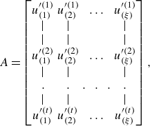 \begin{equation} A = \begin{bmatrix} u'^{(1)}_{(1)} & u'^{(1)}_{(2)} & & \ldots & & u'^{(1)}_{(\xi )} \\ | & |& & & & |\\ | & |& & & & |\\ u'^{(2)}_{(1)} & u'^{(2)}_{(2)} & & \ldots & & u'^{(2)}_{(\xi )} \\ | & |& & & & |\\ . & .& .& .& .& .\\ | & |& & & & |\\ u'^{(t)}_{(1)} & u'^{(t)}_{(2)} & & \ldots & & u'^{(t)}_{(\xi )} \\ \end{bmatrix}, \end{equation}
where $u'^{(i)}_{(j)}$
indicates the streamwise velocity fluctuations in the
$u'^{(i)}_{(j)}$
indicates the streamwise velocity fluctuations in the $i$
th instance in time from the
$i$
th instance in time from the $j$
th ensemble. The POD is performed on this data matrix. The ST-POD mode matrix, upon reshaping, is of size
$j$
th ensemble. The POD is performed on this data matrix. The ST-POD mode matrix, upon reshaping, is of size $[m \times n \times t \times \xi ]$
, where every time instance of the flow has been decomposed into
$[m \times n \times t \times \xi ]$
, where every time instance of the flow has been decomposed into $\xi$
energetically ranked modes. Here [
$\xi$
energetically ranked modes. Here [ $m \times n$
] is the size of the snapshot at time
$m \times n$
] is the size of the snapshot at time $t$
. The resulting modes are coherent in space and in time.
$t$
. The resulting modes are coherent in space and in time.
The spatiotemporal coherence is demonstrated in figure 11, where modes 1 and 5 are shown at five discrete times during the rapid pressure gradient application. Mode 1 is chosen as it is the mode that carries the most energy. Mode 5 is chosen since it has wavelength known to be energetic in TBLs (Marusic et al. Reference Marusic, Monty, Hultmark and Smits2013). Mode 1 (figure 11
a) can be seen to represent a very long structure, estimated from time-correlated snapshots to span $15\delta _0$
. At the instantaneous ZPG condition (figure 11
a–I), the structure appears inclined in the streamwise direction, attached to the wall and concentrated in
$15\delta _0$
. At the instantaneous ZPG condition (figure 11
a–I), the structure appears inclined in the streamwise direction, attached to the wall and concentrated in $y\lt 0.4\delta _0$
. As time progresses, localisation in a thin region close to the wall is seen (for example, in
$y\lt 0.4\delta _0$
. As time progresses, localisation in a thin region close to the wall is seen (for example, in $y\lt 0.15\delta _0$
in figure 11
aIV), outside which the structure appears more diffuse. Changes in the wavelength of this structure are hard to observe since only approximately one average wavelength of the structure is captured in this space–time visualisation. Mode 5 (figure 11
b) shows a modal structure with initial wavelength of
$y\lt 0.15\delta _0$
in figure 11
aIV), outside which the structure appears more diffuse. Changes in the wavelength of this structure are hard to observe since only approximately one average wavelength of the structure is captured in this space–time visualisation. Mode 5 (figure 11
b) shows a modal structure with initial wavelength of $5.5\delta _0$
(judged from figure 11
b–I). In that instance, the structure exhibits a higher inclination angle to the streamwise direction compared with the very long structure captured in figure 11(a). But as the FAPG is rapidly applied, the inclination angle can be seen to decrease, and a localisation in the structure in
$5.5\delta _0$
(judged from figure 11
b–I). In that instance, the structure exhibits a higher inclination angle to the streamwise direction compared with the very long structure captured in figure 11(a). But as the FAPG is rapidly applied, the inclination angle can be seen to decrease, and a localisation in the structure in $y \lt 0.15\delta _0$
is seen to occur.
$y \lt 0.15\delta _0$
is seen to occur.
Space–time POD modes representing structures with initial approximate wavelengths (a) 15 $\delta _0$
and (b) 5.5
$\delta _0$
and (b) 5.5 $\delta _0$
, shown at different time instants in I–V.
$\delta _0$
, shown at different time instants in I–V. $\bar {K}$
= 0, 0.3, 0.6, 0.9 and 1.2 for these instants. As the UPG is applied, the structures are seen to exhibit spatial and temporal changes.
$\bar {K}$
= 0, 0.3, 0.6, 0.9 and 1.2 for these instants. As the UPG is applied, the structures are seen to exhibit spatial and temporal changes.
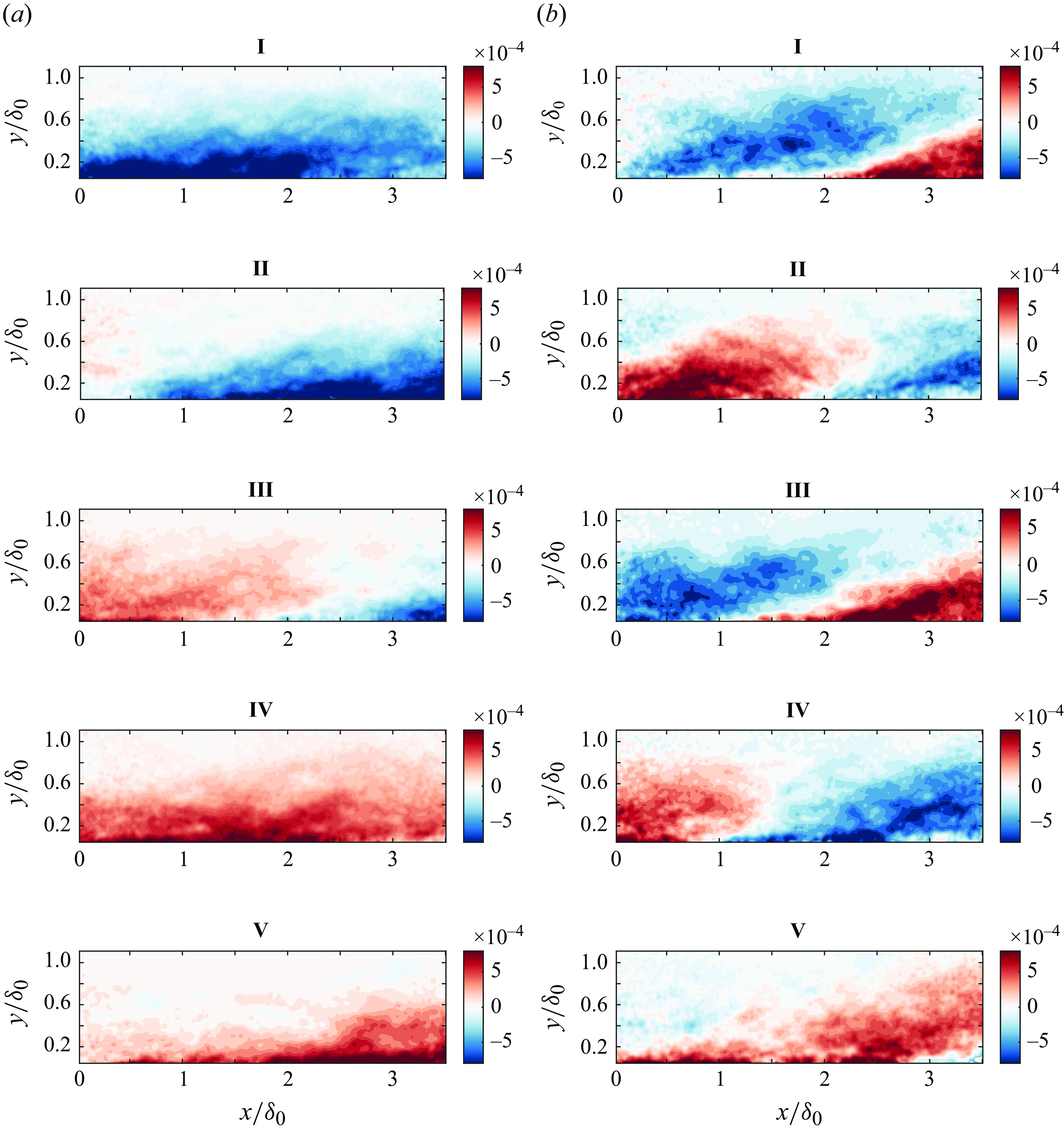
As suggested by figure 11, the structures in the TBL respond to the rapid change in the pressure gradient from the ZPG state ( $\bar {K}$
= 0) to the strongest FAPG state (
$\bar {K}$
= 0) to the strongest FAPG state ( $\bar {K}$
= 1.2) by changing size and shape. Although some of the incurred spatiotemporal changes can be gathered by visually inspecting the modes, the observations can become subjective and it is prohibitively difficult to consolidate these changes in space, in time and across different modes. As before, a comparison with the steady FAPG results is also warranted to separate unsteady effects from the pressure gradient effects, which is also difficult to do in a comprehensive way using visual means. This motivates a framework to quantify modes in terms of the size, angle of inclination and height from the wall, in comparison with the corresponding steady modes. A novel method based on the projection technique used in Saxton-Fox et al. (Reference Saxton-Fox, Lozano-Durán and McKeon2022) is devised.
$\bar {K}$
= 1.2) by changing size and shape. Although some of the incurred spatiotemporal changes can be gathered by visually inspecting the modes, the observations can become subjective and it is prohibitively difficult to consolidate these changes in space, in time and across different modes. As before, a comparison with the steady FAPG results is also warranted to separate unsteady effects from the pressure gradient effects, which is also difficult to do in a comprehensive way using visual means. This motivates a framework to quantify modes in terms of the size, angle of inclination and height from the wall, in comparison with the corresponding steady modes. A novel method based on the projection technique used in Saxton-Fox et al. (Reference Saxton-Fox, Lozano-Durán and McKeon2022) is devised.
Demonstration of the phase-matching approach. (a) The ST-POD structure with approximate wavelength of 4 $\delta _0$
at
$\delta _0$
at $t^*$
= 0 (
$t^*$
= 0 ( $\bar {K}$
= 0). (b) The SPOD structure with the same approximate wavelength and the same spatial pressure gradient (
$\bar {K}$
= 0). (b) The SPOD structure with the same approximate wavelength and the same spatial pressure gradient ( $\bar {K}$
= 0), shown at four phases of its convection. The projection coefficient,
$\bar {K}$
= 0), shown at four phases of its convection. The projection coefficient, $R$
, between (a) and each phase in (b) are labelled on the top right-hand side of the panels, indicating that the SPOD phase in panel IV matches best the phase at which the ST-POD mode is captured in (a).
$R$
, between (a) and each phase in (b) are labelled on the top right-hand side of the panels, indicating that the SPOD phase in panel IV matches best the phase at which the ST-POD mode is captured in (a).
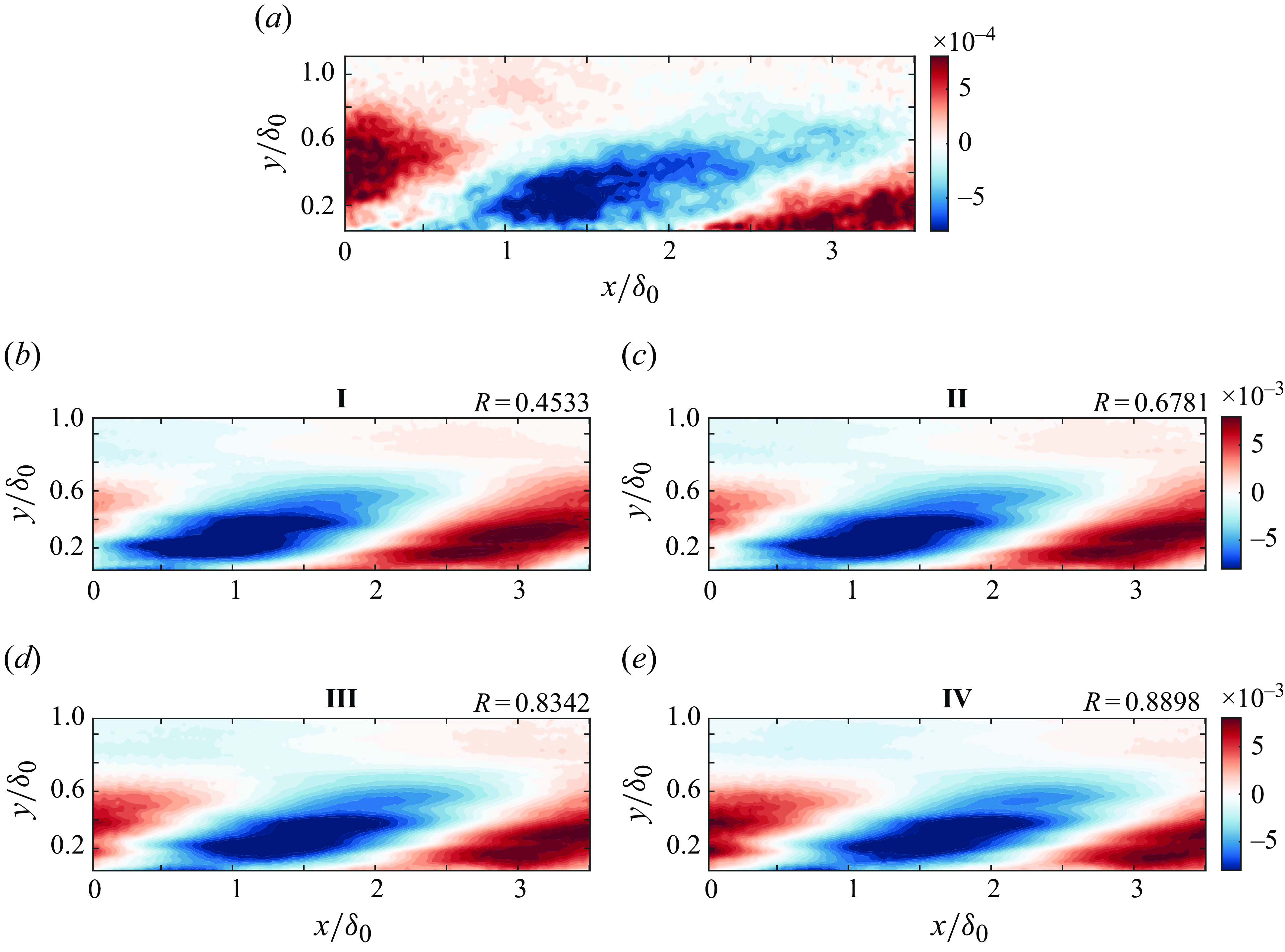
The corresponding steady modal structures are computed from the steady FAPG data using spectral POD (SPOD). The ST-POD modes of the unsteady TBL and the SPOD modes of the steady TBLs at matched FAPG magnitudes are equivalent and comparable because SPOD is the stationary flow (or long-time) formulation of ST-POD, as elucidated by Frame & Towne (Reference Frame and Towne2022). The objectives with the ST-POD modes are two-fold: (i) to quantify the similarities and differences between the steady and unsteady structures at all matched $\bar {K}$
; (ii) to quantify how the structures spatiotemporally deviate from their initial steady-state (given by the SPOD modes at
$\bar {K}$
; (ii) to quantify how the structures spatiotemporally deviate from their initial steady-state (given by the SPOD modes at $\bar {K}$
= 0); if and how the structures transition into their final steady-state (given by the SPOD modes at
$\bar {K}$
= 0); if and how the structures transition into their final steady-state (given by the SPOD modes at $\bar {K}$
= 1.2).
$\bar {K}$
= 1.2).
The phase of an ST-POD structure captured by the PIV FOV changes at every time instance as the structure convects in the flow direction and responds to the pressure gradient. In order to compare an SPOD structure with the ST-POD structure at a given time instance, the phase of the SPOD structure must match the phase of the ST-POD structure captured by that instance. For example, an ST-POD structure with a streamwise wavelength of approximately $4\delta _0$
is shown at
$4\delta _0$
is shown at $t^*$
= 0 (when the pressure gradient is instantaneously zero, or
$t^*$
= 0 (when the pressure gradient is instantaneously zero, or $\bar {K}$
= 0) in figure 12(a). This wavelength is intended to approximate a large-scale structure in the TBL. The chosen instance can be seen to capture the structure at a phase in which the low-speed region occupies most of the FOV, and the front and rear parts of the high-speed region are visible on either side. For an appropriate comparison, the corresponding SPOD structure (
$\bar {K}$
= 0) in figure 12(a). This wavelength is intended to approximate a large-scale structure in the TBL. The chosen instance can be seen to capture the structure at a phase in which the low-speed region occupies most of the FOV, and the front and rear parts of the high-speed region are visible on either side. For an appropriate comparison, the corresponding SPOD structure ( $\bar {K}$
= 0) should also be at the same phase. The structure of a similar wavelength is shown in figure 12(b) at four incremental phases of its convection, computed by leveraging the harmonic nature of SPOD modes. Visually, it is difficult to objectively judge which SPOD phase matches that of the ST-POD mode shown in figure 12(b). A quantitative evaluation of this can be obtained by projecting each SPOD phase onto the ST-POD mode and normalising the projection, as follows:
$\bar {K}$
= 0) should also be at the same phase. The structure of a similar wavelength is shown in figure 12(b) at four incremental phases of its convection, computed by leveraging the harmonic nature of SPOD modes. Visually, it is difficult to objectively judge which SPOD phase matches that of the ST-POD mode shown in figure 12(b). A quantitative evaluation of this can be obtained by projecting each SPOD phase onto the ST-POD mode and normalising the projection, as follows:
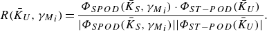 \begin{equation} R(\bar {K}_U,{\gamma _M}_i) = \frac {\Phi _{SPOD} (\bar {K}_S,{\gamma _M}_i) \cdot \Phi _{ST-POD} (\bar {K}_U)}{|\Phi _{SPOD} (\bar {K}_S,{\gamma _M}_i)| |\Phi _{ST-POD} (\bar {K}_U)|}. \end{equation}
Here $\bar {K}_S$
and
$\bar {K}_S$
and $\bar {K}_U$
are the
$\bar {K}_U$
are the $\bar {K}$
that correspond to the considered steady and unsteady structures;
$\bar {K}$
that correspond to the considered steady and unsteady structures; ${\gamma _M}_i$
is the phase angle;
${\gamma _M}_i$
is the phase angle; $\Phi _{SPOD}$
and
$\Phi _{SPOD}$
and $\Phi _{ST-POD}$
are the SPOD and ST-POD modes;
$\Phi _{ST-POD}$
are the SPOD and ST-POD modes; $(\cdot )$
is the dot product;
$(\cdot )$
is the dot product; $(||)$
indicates the norm;
$(||)$
indicates the norm; $R$
is the projection coefficient. Its value is high if the overall similarity (in terms of the shape, size and intensity distribution in space) between the modes compared is high. In the current example,
$R$
is the projection coefficient. Its value is high if the overall similarity (in terms of the shape, size and intensity distribution in space) between the modes compared is high. In the current example, $\bar {K}_S$
and
$\bar {K}_S$
and $\bar {K}_U$
= 0, and four phase angles are considered. The corresponding values of
$\bar {K}_U$
= 0, and four phase angles are considered. The corresponding values of $R$
are shown just above the panels in figure 12(b). Although the SPOD phases considered are visually similar to the ST-POD mode, the projection method can be seen to quantitatively evaluate the differences and produce the largest
$R$
are shown just above the panels in figure 12(b). Although the SPOD phases considered are visually similar to the ST-POD mode, the projection method can be seen to quantitatively evaluate the differences and produce the largest $R$
for phase IV shown in the figure. These phases were specifically chosen to demonstrate the effectiveness of the projection in differentiating between them. If the SPOD structure were considered significantly out of phase with the ST-POD mode at a desired time instance, the projection will yield a negative
$R$
for phase IV shown in the figure. These phases were specifically chosen to demonstrate the effectiveness of the projection in differentiating between them. If the SPOD structure were considered significantly out of phase with the ST-POD mode at a desired time instance, the projection will yield a negative $R$
value.
$R$
value.
In general, for each comparison with an ST-POD structure (say, a given mode at a given time instant), 250 phase shifts in the range 0 $ \lt \gamma _M \lt \pi$
were performed on the SPOD modes and the projection coefficients were obtained for each phase. The phase that results in the maximum
$ \lt \gamma _M \lt \pi$
were performed on the SPOD modes and the projection coefficients were obtained for each phase. The phase that results in the maximum $R$
(
$R$
( $R_{max}$
) is the appropriate phase to compare the SPOD mode with. Since this maximum
$R_{max}$
) is the appropriate phase to compare the SPOD mode with. Since this maximum $R$
already includes the similarities between the ST-POD structure at the given instance and the SPOD structure at a matched pressure gradient condition,
$R$
already includes the similarities between the ST-POD structure at the given instance and the SPOD structure at a matched pressure gradient condition, $R_{max}$
is exactly the quantification sought. Whenever the ST-POD and SPOD modes under comparison are said to be at matched wavelengths in the following discussion, the wavelength-matching has been done visually by choosing the SPOD mode at an appropriate frequency. A more automated approach could also be implemented in future work.
$R_{max}$
is exactly the quantification sought. Whenever the ST-POD and SPOD modes under comparison are said to be at matched wavelengths in the following discussion, the wavelength-matching has been done visually by choosing the SPOD mode at an appropriate frequency. A more automated approach could also be implemented in future work.
The ST-POD structure considered earlier at six discrete time instances (i) and the SPOD structures computed at matched spatial pressure gradient conditions imposed statically (ii). The SPOD mode has been chosen to have the same wavelength as the instantaneous ST-POD structure. The phase has been matched using the method described in the text. Here $\bar {K}$
= 0, 0.25, 0.5, 0.74, 0.96 and 1.2 in (a–f).
$\bar {K}$
= 0, 0.25, 0.5, 0.74, 0.96 and 1.2 in (a–f).
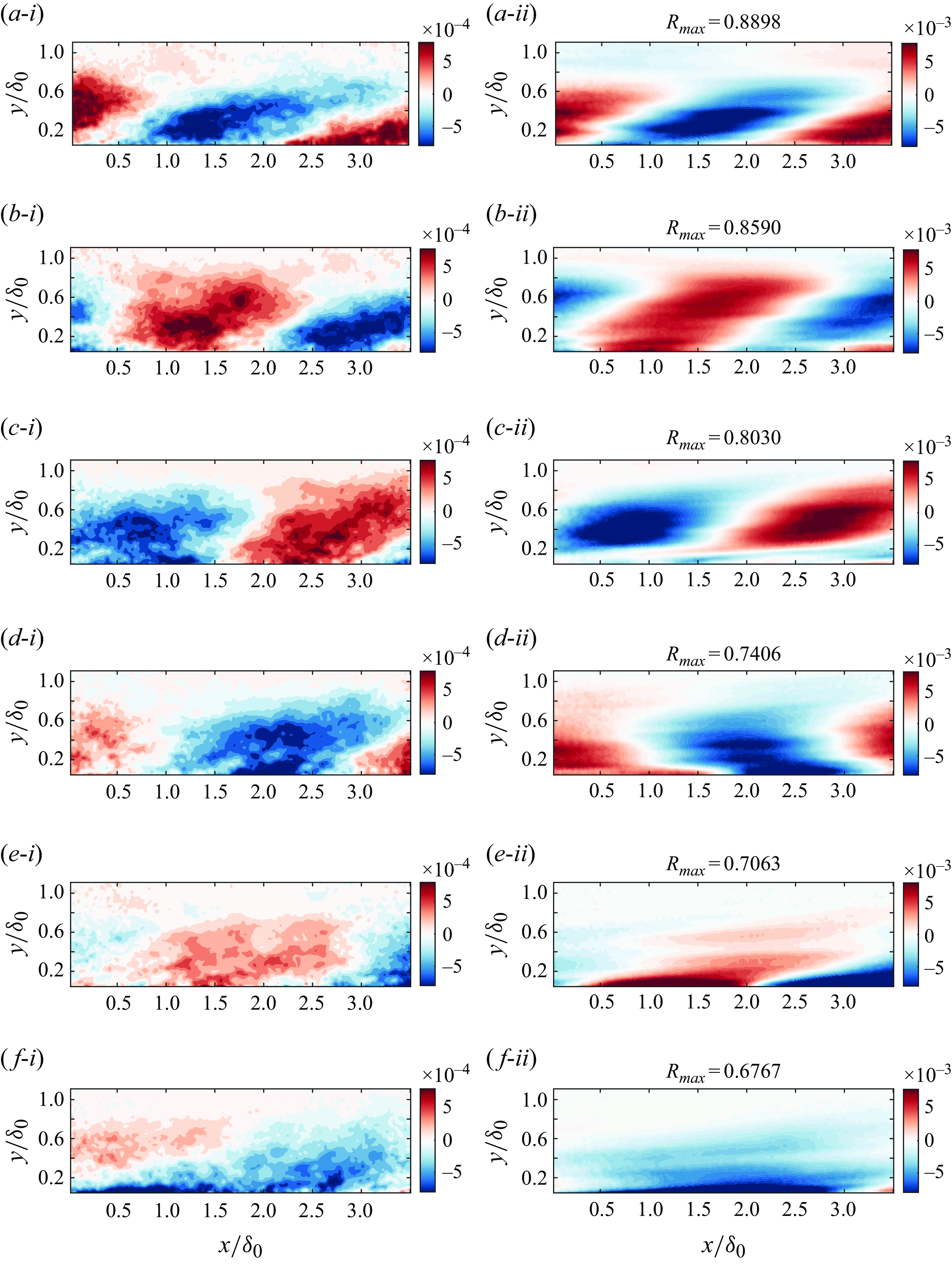
Using this framework, the differences in the response of the large-scale turbulent structures to steady and UPGs of the same magnitude are evaluated. The ST-POD structures of interest are considered at discrete time instances when the pressure gradient magnitude matches the 22 steady pressure gradients imposed (cf. § 2), as done in prior sections. The ST-POD structure with a starting wavelength $\lambda _x$
= 4
$\lambda _x$
= 4 $\delta _0$
at
$\delta _0$
at $t^* = 0$
is shown evolving in time in figure 13(a-i–f-i). The six instances correspond to
$t^* = 0$
is shown evolving in time in figure 13(a-i–f-i). The six instances correspond to $\bar {K}$
= 0, 0.25, 0.5, 0.74, 0.96 and 1. The SPOD structures of matched wavelength and phase at the same
$\bar {K}$
= 0, 0.25, 0.5, 0.74, 0.96 and 1. The SPOD structures of matched wavelength and phase at the same $\bar {K}$
are shown in figure 13(a-ii–f-ii). It can be visually observed that the structures show similar qualitative trends as the pressure gradient magnitude is increased. The structures lengthen and localise near the wall in both figure 13(a-i–f-i) and figure 13(a-ii–f-ii). But the ST-POD modes for the UPG in figure 13(a-i–f-i) show less localisation near the wall in figures 13(e,f) than the equivalent SPOD modes for the stationary case. The projection coefficients quantifying the similarity between figure 13(a-i–f-i) and figure 13(a-ii–f-ii) (ST-POD versus SPOD) in the same row (same pressure gradient) are labelled on top of each panel in figure 13(a-ii–f-ii). A trend emerges, which suggests that the deviation of the unsteady response to the corresponding steady response increases with time. Such a quantification was done by setting
$\bar {K}$
are shown in figure 13(a-ii–f-ii). It can be visually observed that the structures show similar qualitative trends as the pressure gradient magnitude is increased. The structures lengthen and localise near the wall in both figure 13(a-i–f-i) and figure 13(a-ii–f-ii). But the ST-POD modes for the UPG in figure 13(a-i–f-i) show less localisation near the wall in figures 13(e,f) than the equivalent SPOD modes for the stationary case. The projection coefficients quantifying the similarity between figure 13(a-i–f-i) and figure 13(a-ii–f-ii) (ST-POD versus SPOD) in the same row (same pressure gradient) are labelled on top of each panel in figure 13(a-ii–f-ii). A trend emerges, which suggests that the deviation of the unsteady response to the corresponding steady response increases with time. Such a quantification was done by setting $\bar {K}_S = \bar {K}_U$
in (4.2) for each of the 22 pressure gradients and for three ST-POD large-scale structures with initial wavelengths
$\bar {K}_S = \bar {K}_U$
in (4.2) for each of the 22 pressure gradients and for three ST-POD large-scale structures with initial wavelengths $4-7 \delta _0$
. The results were averaged across the modes and are shown in figure 14. The trend is clear in showing that the unsteady large scales are initially highly similar to the steady large scales under matched pressure gradient magnitudes, but that similarity progressively decreases with time as the pressure gradient strengthens.
$4-7 \delta _0$
. The results were averaged across the modes and are shown in figure 14. The trend is clear in showing that the unsteady large scales are initially highly similar to the steady large scales under matched pressure gradient magnitudes, but that similarity progressively decreases with time as the pressure gradient strengthens.
Structural differences between unsteady large scales of wavelength $3-7\delta _0$
and corresponding steady large scales of matched wavelengths, as the pressure gradient is dynamically increased in the former and statically increased in the latter.
$3-7\delta _0$
and corresponding steady large scales of matched wavelengths, as the pressure gradient is dynamically increased in the former and statically increased in the latter.

The manner of deviation of a large-scale structure from its initial steady-state as the pressure gradient strengthens in time, and the manner of its transition to the final steady-state in time are studied. The same ST-POD structure as in figure 12 (with $\lambda _x \equiv 4\delta _0$
) is considered. The SPOD mode in case
$\lambda _x \equiv 4\delta _0$
) is considered. The SPOD mode in case $\bar {K}$
= 0 whose wavelength matches the ST-POD structure at
$\bar {K}$
= 0 whose wavelength matches the ST-POD structure at $\bar {K}$
= 0 is considered for comparison with the initial steady-state. The SPOD mode in case
$\bar {K}$
= 0 is considered for comparison with the initial steady-state. The SPOD mode in case $\bar {K}$
= 1.2 whose wavelength matches the ST-POD structure at
$\bar {K}$
= 1.2 whose wavelength matches the ST-POD structure at $\bar {K}$
= 1.2 is considered for the comparison with the final steady-state. At every time instance,
$\bar {K}$
= 1.2 is considered for the comparison with the final steady-state. At every time instance, $R_{max}$
is obtained by matching the phase of the SPOD structure to the phase that the ST-POD structure is captured at in that time instance. Tracking the
$R_{max}$
is obtained by matching the phase of the SPOD structure to the phase that the ST-POD structure is captured at in that time instance. Tracking the $R_{max}$
that results from the comparison with the initial steady-state as a function of the non-dimensional time is shown in figure 15(a), where
$R_{max}$
that results from the comparison with the initial steady-state as a function of the non-dimensional time is shown in figure 15(a), where $\bar {K}_U$
in (4.2) is varied from 0 to 1.2 while holding
$\bar {K}_U$
in (4.2) is varied from 0 to 1.2 while holding $\bar {K}_S = 0$
. The deviation from the final steady-state is shown in figure 15(b), where
$\bar {K}_S = 0$
. The deviation from the final steady-state is shown in figure 15(b), where $\bar {K}_U$
in (4.2) is varied from 0 to 1.2 while holding
$\bar {K}_U$
in (4.2) is varied from 0 to 1.2 while holding $\bar {K}_S = 1.2$
. At the beginning of unsteady time, when the TBL is at an instantaneous ZPG, the figures show that the large-scale structure in the unsteady TBL is highly similar to that in the steady ZPG TBL (
$\bar {K}_S = 1.2$
. At the beginning of unsteady time, when the TBL is at an instantaneous ZPG, the figures show that the large-scale structure in the unsteady TBL is highly similar to that in the steady ZPG TBL ( $R_{max} = 0.89$
, figure 15
a) but highly dissimilar to that in the steady FAPG TBL with
$R_{max} = 0.89$
, figure 15
a) but highly dissimilar to that in the steady FAPG TBL with $\bar {K} = 1.2$
(
$\bar {K} = 1.2$
( $R_{max} = 0.37$
, figure 15
b). As time progresses and the structures respond to the temporally strengthening pressure gradient, the unsteady structure slowly loses similarity to the steady ZPG structure and slowly gains similarity with the steady FAPG structure. At the end of unsteady time, when the TBL is instantaneously under a strong FAPG with
$R_{max} = 0.37$
, figure 15
b). As time progresses and the structures respond to the temporally strengthening pressure gradient, the unsteady structure slowly loses similarity to the steady ZPG structure and slowly gains similarity with the steady FAPG structure. At the end of unsteady time, when the TBL is instantaneously under a strong FAPG with $\bar {K}$
= 1.2, the projection with the steady ZPG gives
$\bar {K}$
= 1.2, the projection with the steady ZPG gives $R_{max} = 0.48$
and the projection with the steady FAPG of the same magnitude gives
$R_{max} = 0.48$
and the projection with the steady FAPG of the same magnitude gives $R_{max} = 0.67$
. While the low correlation with the ZPG is consistent with what is expected, the similarity with the steady FAPG is found to only be moderate, suggesting that the unsteady structures respond differently to the same pressure gradient magnitude than the corresponding steady structures, as also shown by figure 14. Another interesting observation is the manner of deviation of the unsteady structure from its initial steady state: although the deviation generally progressively increases, the rate is initially slow (
$R_{max} = 0.67$
. While the low correlation with the ZPG is consistent with what is expected, the similarity with the steady FAPG is found to only be moderate, suggesting that the unsteady structures respond differently to the same pressure gradient magnitude than the corresponding steady structures, as also shown by figure 14. Another interesting observation is the manner of deviation of the unsteady structure from its initial steady state: although the deviation generally progressively increases, the rate is initially slow ( $t^* \lt$
0.75), suggesting some resistance of the structure to the temporal pressure gradient change.
$t^* \lt$
0.75), suggesting some resistance of the structure to the temporal pressure gradient change.
Quantification of the temporal changes underwent by an unsteady ST-POD structure under the dynamic pressure gradient imposition. (a) Changes away from the initial steady-state (ZPG) of a large-scale ST-POD structure as the pressure gradient strengthens in time. The initial steady-state structure is given by an SPOD mode at $\bar {K} = 0$
with matched ZPG wavelength. (b) Changes towards the final steady-state (strong FAPG) of the same ST-POD structure as the pressure gradient strengthens in time. An SPOD mode at
$\bar {K} = 0$
with matched ZPG wavelength. (b) Changes towards the final steady-state (strong FAPG) of the same ST-POD structure as the pressure gradient strengthens in time. An SPOD mode at $\bar {K}$
= 1.2 with matched FAPG wavelength serves as the final steady-state structure.
$\bar {K}$
= 1.2 with matched FAPG wavelength serves as the final steady-state structure.
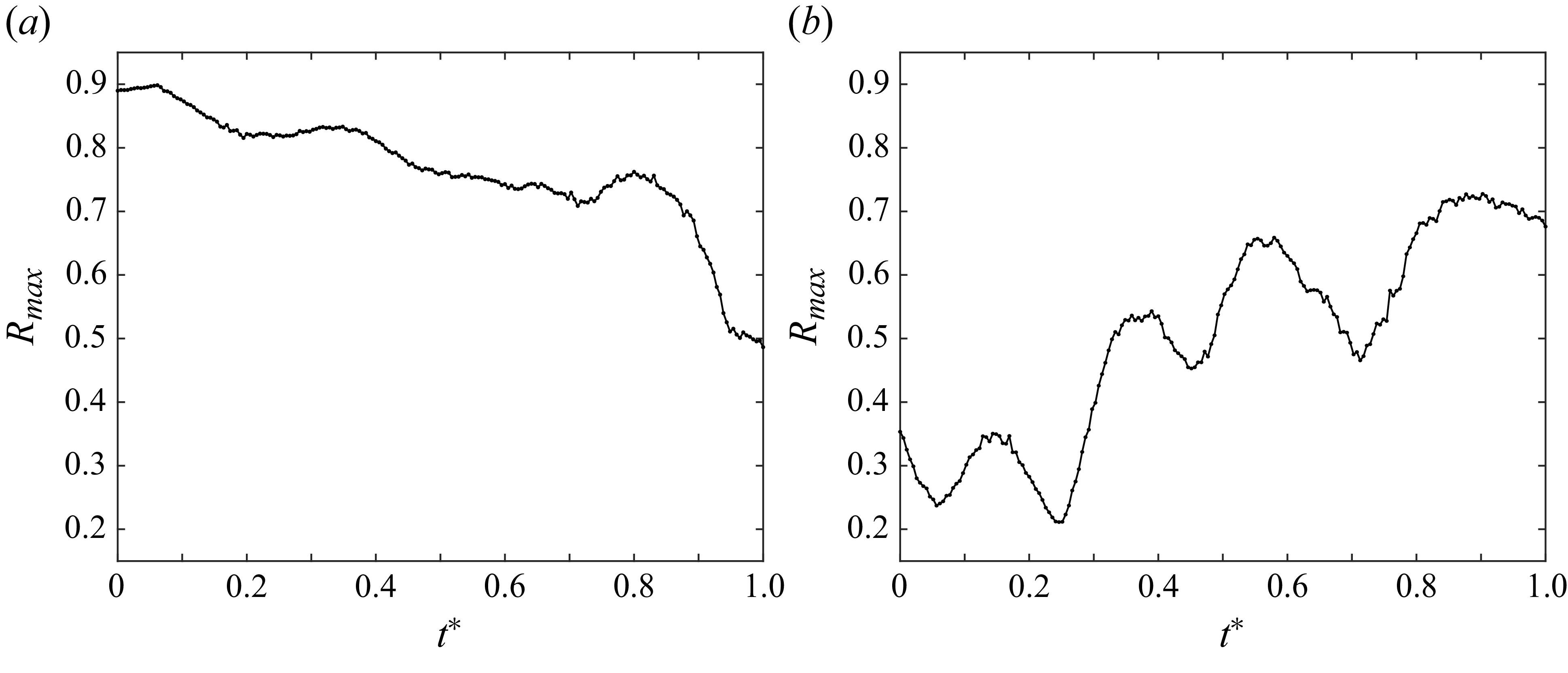
Both trends shown in figure 15 were found to be consistent across modes with initial $\lambda _x$
=
$\lambda _x$
= $4-12\delta _0$
. The undulations in
$4-12\delta _0$
. The undulations in $R_{max}$
with
$R_{max}$
with $t^*$
likely appeared because of the mismatch of wavelength between the SPOD and STPOD modes considered and because of the convection of the structure in and out of the PIV FOV: whenever both the positive and negative regions of the structure were captured in the FOV, the
$t^*$
likely appeared because of the mismatch of wavelength between the SPOD and STPOD modes considered and because of the convection of the structure in and out of the PIV FOV: whenever both the positive and negative regions of the structure were captured in the FOV, the $R_{max}$
was higher and if the FOV was occupied by fully positive or fully negative structures, the
$R_{max}$
was higher and if the FOV was occupied by fully positive or fully negative structures, the $R_{max}$
was lower. It is estimated that these undulations would be alleviated if the streamwise extent of the FOV was twice the wavelength of the longest structure considered. In that case, both positive and negative regions of the structure would always be captured in the FOV. That is why, for example, the undulations in figure 15(a) is weaker than that in figure 15(b), since the wavelength of the structure at the ZPG condition was
$R_{max}$
was lower. It is estimated that these undulations would be alleviated if the streamwise extent of the FOV was twice the wavelength of the longest structure considered. In that case, both positive and negative regions of the structure would always be captured in the FOV. That is why, for example, the undulations in figure 15(a) is weaker than that in figure 15(b), since the wavelength of the structure at the ZPG condition was $\lambda _x \equiv 4\delta _0$
(14
$\lambda _x \equiv 4\delta _0$
(14 $\, \%$
longer than the FOV), which then increased to
$\, \%$
longer than the FOV), which then increased to $\lambda _x \equiv 7\delta _0$
(100
$\lambda _x \equiv 7\delta _0$
(100 $\, \%$
longer than the FOV) as the pressure gradient increased in time. Nonetheless, the trends exhibited are useful as they quantitatively capture the transient/dynamic changes in shape, wavelength, angle of inclination and height from the wall, undergone by the turbulent structure. Such quantitative tracking that simultaneously leverages spatial and temporal information about changes undergone by structures in the TBL makes the developed method powerful.
$\, \%$
longer than the FOV) as the pressure gradient increased in time. Nonetheless, the trends exhibited are useful as they quantitatively capture the transient/dynamic changes in shape, wavelength, angle of inclination and height from the wall, undergone by the turbulent structure. Such quantitative tracking that simultaneously leverages spatial and temporal information about changes undergone by structures in the TBL makes the developed method powerful.
5. Discussion
The statistical and modal analyses carried out in this work suggest that the unsteady/transient FAPG imposition does not elicit a pseudosteady response from the TBL. While under the steady pressure gradient imposition, discussed in Parthasarathy & Saxton-Fox (Reference Parthasarathy and Saxton-Fox2023), the upstream FPG strongly stabilised the turbulence and yielded a milder APG response in the downstream APG region, a different trend is observed when the same FAPG is applied rapidly. Surprisingly, a milder stabilisation at the exit of the FPG region results, despite the expectation that the added temporal acceleration would act to reinforce FPG effects. This less-stabilised unsteady TBL responds more strongly to the following APG, showing traits in between traditional ZAPG response and the coupled FAPG response seen in the steady cases. The small outer peaks in turbulent statistics are characteristic of the former and the formation of a (weaker) internal layer is that of the latter.
A hypothesis for the observed dynamic effects is developed based on the following premise: since the pressure gradient imposition in the unsteady case happens at a time scale relevant to that of turbulent structures ( $k_\tau$
= 1.79), the structures feel the spatial pressure gradients changing and hence experience a different spatiotemporal pressure gradient history before reaching a given location of interest than they do in the steady cases. This difference in the pressure gradient history is suggested to contribute to the differences observed in the steady and unsteady responses.
$k_\tau$
= 1.79), the structures feel the spatial pressure gradients changing and hence experience a different spatiotemporal pressure gradient history before reaching a given location of interest than they do in the steady cases. This difference in the pressure gradient history is suggested to contribute to the differences observed in the steady and unsteady responses.
To test the hypothesis, the pressure gradients experienced by the structures as they convect past the test area during the temporal ceiling deformation are computed in a Lagrangian frame of reference fixed on the structures. The available geometric states of the ceiling during its deformation (figure 1
b) and the estimated pressure gradient variation associated with each ceiling state (figure 2
a) are leveraged for this analysis. The convection speed, $U_c(x,t)$
, was assumed to be 0.82
$U_c(x,t)$
, was assumed to be 0.82 $U_e(x,t)$
, which was manually estimated from the convection of the ST-POD structures and is similar to that used in the literature for large scales in the outer region. A convection velocity of 0.5
$U_e(x,t)$
, which was manually estimated from the convection of the ST-POD structures and is similar to that used in the literature for large scales in the outer region. A convection velocity of 0.5 $U_e(x,t)$
has also been considered to demonstrate the conditions experienced by structures convecting at a different speed.
$U_e(x,t)$
has also been considered to demonstrate the conditions experienced by structures convecting at a different speed.
The instantaneous pressure gradient experienced by the structure is computed as
 \begin{equation} K(t^*) = K(U_c \times \Delta t^*, t^*), \end{equation}
which tracks the temporal history of the spatial pressure gradient experienced by the structure as it convects. Here $U_c$
is computed as the convection velocity at the previous time step: 0.82
$U_c$
is computed as the convection velocity at the previous time step: 0.82 $U_e(x(t^*-\Delta t^*),t^* - \Delta t^*)$
. The equivalent spatial picture, i.e. the spatial pressure gradient local to space as the structure convects, is obtained from
$U_e(x(t^*-\Delta t^*),t^* - \Delta t^*)$
. The equivalent spatial picture, i.e. the spatial pressure gradient local to space as the structure convects, is obtained from $K(t^*)$
using the convection velocity as
$K(t^*)$
using the convection velocity as
 \begin{equation} K(x') = K(t^* \times U_c). \end{equation}
The pressure gradient history experienced by a structure by the time it reaches station $A$
at the end of unsteady time (
$A$
at the end of unsteady time ( $t^* = 1$
or
$t^* = 1$
or $\bar {K}$
= 1.2, and contributes to the corresponding flow behaviours observed at station
$\bar {K}$
= 1.2, and contributes to the corresponding flow behaviours observed at station $A$
) is shown in red in figure 16(a). The same is shown in red for station
$A$
) is shown in red in figure 16(a). The same is shown in red for station $B$
in figure 16(c). In the same figures, the pressure gradient history experienced by the structure if the ceiling was held statically at the final state (
$B$
in figure 16(c). In the same figures, the pressure gradient history experienced by the structure if the ceiling was held statically at the final state ( $\bar {K}$
= 1.2) instead of being dynamically imposed, is also shown in black.
$\bar {K}$
= 1.2) instead of being dynamically imposed, is also shown in black.
Temporal history of the spatial pressure gradient experienced by structures when observed from a Lagrangian frame of reference fixed on the structures. (a,b) Here $K$
experienced by structures that reach station
$K$
experienced by structures that reach station $A$
when
$A$
when $\bar {K}$
= 1.2 (fully deflected ceiling state); (c,d)
$\bar {K}$
= 1.2 (fully deflected ceiling state); (c,d) $K$
experienced by structures that reach station
$K$
experienced by structures that reach station $B$
when
$B$
when $\bar {K}$
= 1.2. Convection speed of the structures
$\bar {K}$
= 1.2. Convection speed of the structures $U_c$
= 0.82
$U_c$
= 0.82 $U_e(x,t)$
in (a,c) and
$U_e(x,t)$
in (a,c) and $U_c$
= 0.5
$U_c$
= 0.5 $U_e(x,t)$
in (b,d). The legend shows the assumed time scales of the UPG impositions.
$U_e(x,t)$
in (b,d). The legend shows the assumed time scales of the UPG impositions. $t_f$
= 0.07 is the one relevant to this work, whereas the other
$t_f$
= 0.07 is the one relevant to this work, whereas the other $t_f$
are supposed.
$t_f$
are supposed.

At station $A$
, when the ceiling is static at its fully deflected state, the structure experiences a spatially weakening FPG variation associated with that ceiling geometry, varying from
$A$
, when the ceiling is static at its fully deflected state, the structure experiences a spatially weakening FPG variation associated with that ceiling geometry, varying from $K = 6 \times 10^{-6}$
at
$K = 6 \times 10^{-6}$
at $x/L_C = 0$
to
$x/L_C = 0$
to $K \approx 0$
at
$K \approx 0$
at $x/L_C = 0.5$
, exactly as shown in figure 2(b). This is conveyed by the black line. When the ceiling unsteadily deforms to the same fully deflected state, however, the
$x/L_C = 0.5$
, exactly as shown in figure 2(b). This is conveyed by the black line. When the ceiling unsteadily deforms to the same fully deflected state, however, the $K$
variation experienced by the unsteady structure before it reaches station
$K$
variation experienced by the unsteady structure before it reaches station $A$
is seen to be considerably milder. The maximum
$A$
is seen to be considerably milder. The maximum $K$
it experiences is
$K$
it experiences is $1.3 \times 10^{-6}$
. At station
$1.3 \times 10^{-6}$
. At station $B$
(figure 16
c), a steady structure that reaches this station when the ceiling is fully deflected (and held static) experiences the FPG-APG associated with this geometry, varying from
$B$
(figure 16
c), a steady structure that reaches this station when the ceiling is fully deflected (and held static) experiences the FPG-APG associated with this geometry, varying from $K = 6 \times 10^{-6}$
at
$K = 6 \times 10^{-6}$
at $x/L_C = 0$
to
$x/L_C = 0$
to $K \approx 0$
at
$K \approx 0$
at $x/L_C = 0.5$
to
$x/L_C = 0.5$
to $K = -4.8 \times 10^{-6}$
at
$K = -4.8 \times 10^{-6}$
at $x/L_C = 0.81$
, as shown by the black line. But the unsteady structure that reaches this station at the end of unsteady time can be seen to have hardly experienced the FPG imposed upstream. The structure reaches station
$x/L_C = 0.81$
, as shown by the black line. But the unsteady structure that reaches this station at the end of unsteady time can be seen to have hardly experienced the FPG imposed upstream. The structure reaches station $B$
with a history of being in a weak FPG and in a strengthening APG.
$B$
with a history of being in a weak FPG and in a strengthening APG.
These histories at stations $A$
and
$A$
and $B$
(and at in-between stations not shown) are reflective of the facts that a spatially weakening FPG followed by a spatially strengthening APG is imposed on the boundary layer by virtue of the chosen geometry, but the relative time scale between the geometry deformation and the convection of the structures is such that the structures end up in the APG region before the strong FPG is imposed on the flat plate. Hence, the unsteady structures experience the APG, but only mildly the upstream FPG. It follows, then, that if the relative time scale between the deformation and the convection of the structures varies, the spatiotemporal pressure gradient history, and hence the TBL response, would vary. The blue, green and magenta lines in figure 16(a) and figure 16(c) correspond to scenarios with different deformation time scales:
$B$
(and at in-between stations not shown) are reflective of the facts that a spatially weakening FPG followed by a spatially strengthening APG is imposed on the boundary layer by virtue of the chosen geometry, but the relative time scale between the geometry deformation and the convection of the structures is such that the structures end up in the APG region before the strong FPG is imposed on the flat plate. Hence, the unsteady structures experience the APG, but only mildly the upstream FPG. It follows, then, that if the relative time scale between the deformation and the convection of the structures varies, the spatiotemporal pressure gradient history, and hence the TBL response, would vary. The blue, green and magenta lines in figure 16(a) and figure 16(c) correspond to scenarios with different deformation time scales: $t_f$
= 0.15 s, 0.32 s and 0.86 s, respectively. Figure 16(b) and figure 16(d) are similar to figure 16(a) and figure 16(c), but with the convection speed changed to
$t_f$
= 0.15 s, 0.32 s and 0.86 s, respectively. Figure 16(b) and figure 16(d) are similar to figure 16(a) and figure 16(c), but with the convection speed changed to $U_c$
= 0.5
$U_c$
= 0.5 $U_e(x,t)$
. It can be seen that decreasing the unsteady time scale causes the pressure gradient history to tend towards the steady pressure gradient history (given by the black line). This is in line with an expectation that in the limit of a very slow deformation of the ceiling, the TBL response would be quasisteady. When the structures convect at a slower time scale (figure 16
b,d), the pressure gradient history is similar to the ceiling moving faster. As mentioned earlier, it is the relative time scale that governs the history.
$U_e(x,t)$
. It can be seen that decreasing the unsteady time scale causes the pressure gradient history to tend towards the steady pressure gradient history (given by the black line). This is in line with an expectation that in the limit of a very slow deformation of the ceiling, the TBL response would be quasisteady. When the structures convect at a slower time scale (figure 16
b,d), the pressure gradient history is similar to the ceiling moving faster. As mentioned earlier, it is the relative time scale that governs the history.
Spatial distribution of the pressure gradient history experienced by structures when observed from a Lagrangian frame of reference fixed on the structures, expanding on the temporal picture in figure 16(a,b) Here $K$
experienced by structures that reach station
$K$
experienced by structures that reach station $A$
when
$A$
when $\bar {K}$
= 1.2 (fully deflected ceiling state), and (c,d)
$\bar {K}$
= 1.2 (fully deflected ceiling state), and (c,d) $K$
experienced by structures that reach station
$K$
experienced by structures that reach station $B$
when
$B$
when $\bar {K}$
= 1.2. Convection speed of the structures is
$\bar {K}$
= 1.2. Convection speed of the structures is $U_c = 0.82 U_e(x,t)$
in (a,c) and
$U_c = 0.82 U_e(x,t)$
in (a,c) and $U_c = 0.5 U_e(x,t)$
in (b,d).
$U_c = 0.5 U_e(x,t)$
in (b,d).
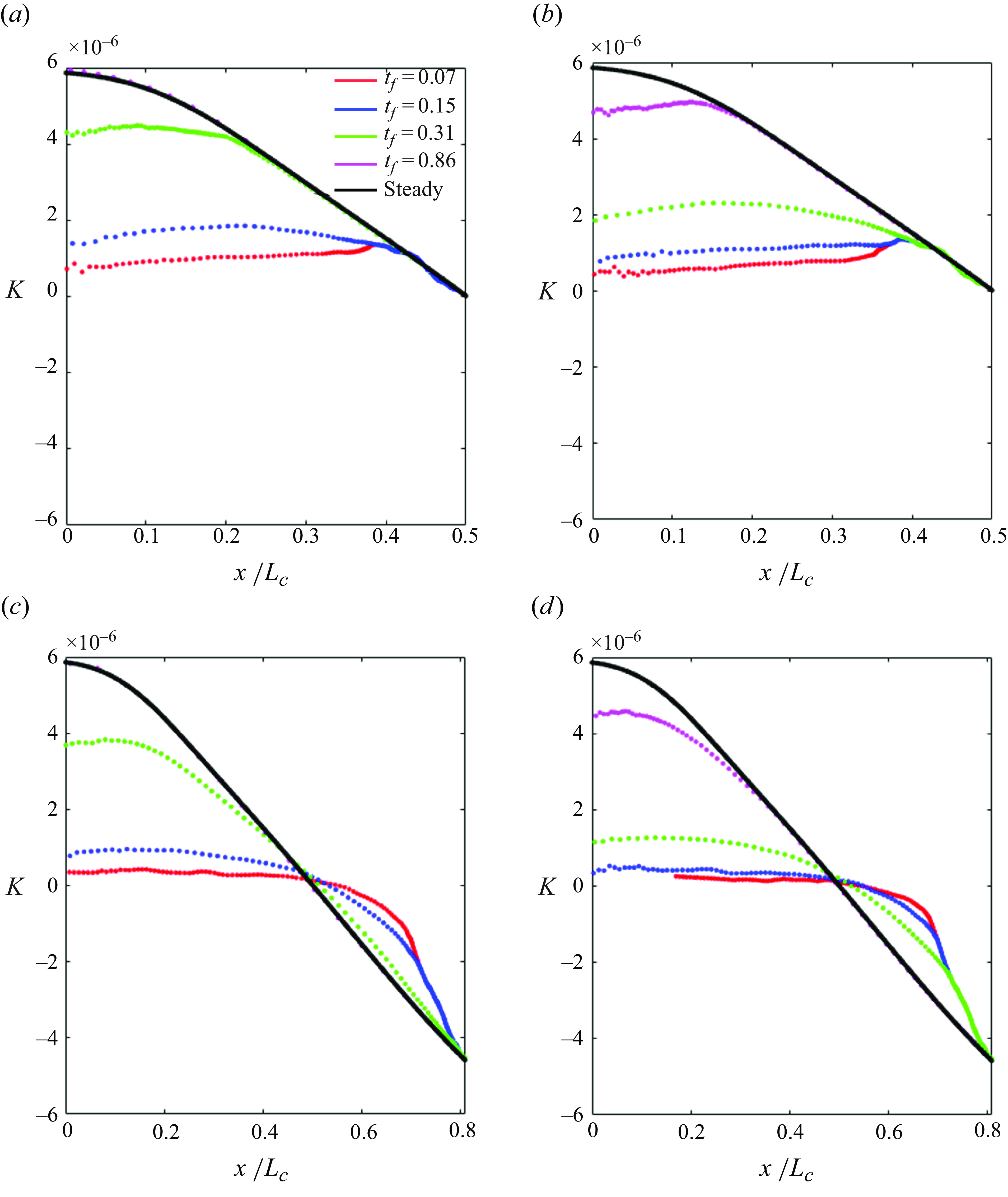
The spatial picture equivalent to figure 16 is shown in figure 17, which visually brings out the difference in history for different unsteadiness time scales more starkly. By mapping the temporal history of the pressure gradients to the spatial domain, this figure illustrates where in space the structure encounters each segment of its $K$
history. This perspective makes it easier to visualise the evolving influence of the pressure gradients as the structures convect through the domain. In figure 17(a), for example, a structure with a convection velocity of 0.82
$K$
history. This perspective makes it easier to visualise the evolving influence of the pressure gradients as the structures convect through the domain. In figure 17(a), for example, a structure with a convection velocity of 0.82 $U_e$
only experiences a mild FPG throughout the FPG region, and reaches station
$U_e$
only experiences a mild FPG throughout the FPG region, and reaches station $A$
with this mild FPG history. This reflects the fact that the rapid ceiling deformation prevents the structure, convecting at a comparable speed as the ceiling deformation, from fully experiencing the upstream FPG. As the unsteadiness time scale increases, however, the spatial history more closely resembles the steady pressure gradient profile. In figure 17(c,d), it can be seen that the structures experience the full extent of the APG applied, but the spatial rate of change is greater for faster unsteady time scales. So the unsteady structures see a more rapid spatial change in the pressure gradients they experience.
$A$
with this mild FPG history. This reflects the fact that the rapid ceiling deformation prevents the structure, convecting at a comparable speed as the ceiling deformation, from fully experiencing the upstream FPG. As the unsteadiness time scale increases, however, the spatial history more closely resembles the steady pressure gradient profile. In figure 17(c,d), it can be seen that the structures experience the full extent of the APG applied, but the spatial rate of change is greater for faster unsteady time scales. So the unsteady structures see a more rapid spatial change in the pressure gradients they experience.
This hypothesis that a different spatiotemporal pressure gradient history is the source of the unsteady effect helps in rationalising the intriguing trends observed in the unsteady response. The structures that reach any location of interest always come with a milder FAPG history than they would have in the steady case, hence causing milder FPG effects at station $A$
despite the added temporal acceleration, followed by less coupled FAPG effects at station
$A$
despite the added temporal acceleration, followed by less coupled FAPG effects at station $B$
. Furthermore, the estimates of the spatiotemporal histories of the structures show that they would tend towards the spatial history in a corresponding steady case at low time scales, leading to a quasisteady response. This was observed heuristically to be true in a different set of experiments where the pressure gradients were imposed less rapidly (
$B$
. Furthermore, the estimates of the spatiotemporal histories of the structures show that they would tend towards the spatial history in a corresponding steady case at low time scales, leading to a quasisteady response. This was observed heuristically to be true in a different set of experiments where the pressure gradients were imposed less rapidly ( $t_f$
= 0.2 s, instead of
$t_f$
= 0.2 s, instead of $t_f$
= 0.07 s here), where an almost quasisteady behaviour was exhibited by the statistics.
$t_f$
= 0.07 s here), where an almost quasisteady behaviour was exhibited by the statistics.
Schematic of the hypothesis presented. (a) Structures under the different steady pressure gradient impositions always experience the same pressure gradient history before reaching the FOV (shown by the green box). (b) Structures under the UPG imposition reach the FOV with a pressure gradient history that depends on how quickly the structures move relative to how quickly the ceiling deforms. The history shown here is representative of the unsteady case studied in this chapter, where the structures tend to convect into the FOV before getting to experience the strong upstream FPG.
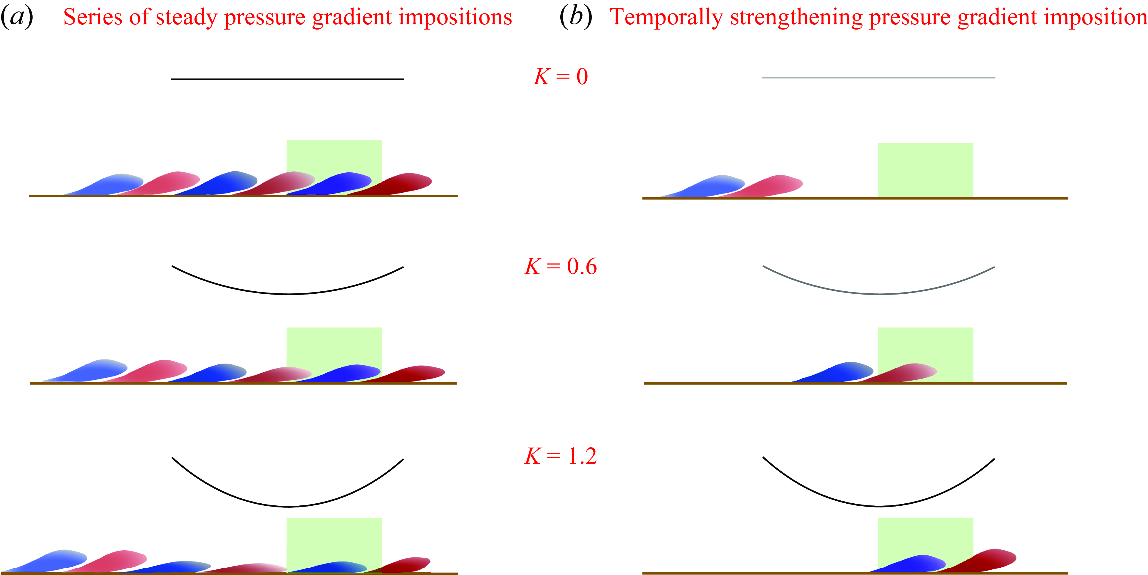
A schematic representation of the hypothesis is shown in figure 18, where the spatial pressure gradients experienced by structures under a series of steady FAPG impositions are compared with that under a temporal FAPG imposition. In the steady cases, the structures feel the full extent of the FAPG imposed in each, but in the unsteady case, the structures convect as the FAPG changes and feel a milder FAPG history as a result.
The main simplifying assumption involved in formulating this hypothesis is that only the convection speeds of the structures are taken to matter, not their phase or wavelength. No significant evidence has so far pointed to different responses by positive/negative phases of the structures to the steady or UPGs imposed. The wavelength, however, can be expected to matter: there is literature evidence that large scales respond more strongly to pressure gradients than small scales. Additionally, the hypothesis does not explicitly include the temporal acceleration effect, which is closely linked to the spatial acceleration caused by the upstream FPG. The temporal acceleration would act to strengthen and weaken, respectively, the FPG and APG effects, but in a milder manner than a spatial acceleration would. This still supports the suggestions of the current hypothesis. In any case, the hypothesis presents a viable (even if simplified) picture of the source of differences in the flow physics observed.
The Lagrangian perspective could be used to define a parameter that may yield a collapse between unsteady and stationary data, but we highlight two challenges that prevent us from attempting such a collapse in this manuscript. First, the variable convection speed present in the boundary layer means that different regions of the boundary layer will experience different Lagrangian pressure gradient trajectories, complicating comparisons between stationary and unsteady geometries. Second, it is a significant challenge in stationary geometries to identify scaling parameters for flows that experience rapid changes in the pressure gradient from favourable to adverse in sequence Parthasarathy & Saxton-Fox (Reference Parthasarathy and Saxton-Fox2023). As future work, it may be fruitful to attempt to collapse stationary and unsteady data with a purely favourable or purely APG first.
6. Conclusion
The statistics and structure of the TBL as the pressure gradient on a flat plate was changed from ZPG condition to a strong FAPG condition within a duration of 0.07 s were studied. By comparing the unsteady TBL with a series of steady TBLs at matched pressure gradient conditions (i.e. matched states of the ceiling), the effect of unsteadiness was isolated from the effects of the spatial pressure gradients. Throughout the dynamic pressure gradient imposition, the unsteady TBL showed several features of the corresponding steady TBL, which suggests that the spatial pressure gradients have a more dominating effect on the boundary layer compared with the unsteadiness. However, significant unsteady effects were also observed. Most notably, the unsteady FAPG imposition elicited a milder effect of the upstream FPG from the TBL and subsequently, a stronger effect of the downstream APG, when compared with an equivalent steady FAPG imposition.
In the statistics, at the upstream end of the FOV where the TBL has undergone a temporally strengthening FPG region, the mean and Reynolds stresses initially overshot the corresponding steady profiles and then undershot them. Instead of the double peak structure seen in the steady FAPG cases, which was a signature of an internal layer, the statistics exhibited a single peak. A double peak structure later developed around $x/L_x \sim 0.35$
. As in the steady TBLs, the first peak grew in
$x/L_x \sim 0.35$
. As in the steady TBLs, the first peak grew in $x$
, associated with the streamwise growth of the internal layer, but the growth rate was lower for the unsteady case such that the peak magnitude was lower at the downstream end of the FOV. Concurrently, the peak strength and population of vortices near the wall due to the internal layer were also present in the unsteady case, but lower in magnitude than corresponding steady cases. While the outer peaks in the steady FAPGs diminished with increasing
$x$
, associated with the streamwise growth of the internal layer, but the growth rate was lower for the unsteady case such that the peak magnitude was lower at the downstream end of the FOV. Concurrently, the peak strength and population of vortices near the wall due to the internal layer were also present in the unsteady case, but lower in magnitude than corresponding steady cases. While the outer peaks in the steady FAPGs diminished with increasing $x$
, the unsteady FAPG showed mildly strengthening outer peaks in the Reynolds stresses and the vortex populations that left the boundary layer with prominent outer peaks at the end of the APG region recorded. This was surprising because the corresponding steady pressure gradient case showed no outer peak, which was attributed to the strong stabilising effect of the upstream FPG and the presence of the internal layer within which the stress-producing large scales were confined (Parthasarathy & Saxton-Fox Reference Parthasarathy and Saxton-Fox2023).
$x$
, the unsteady FAPG showed mildly strengthening outer peaks in the Reynolds stresses and the vortex populations that left the boundary layer with prominent outer peaks at the end of the APG region recorded. This was surprising because the corresponding steady pressure gradient case showed no outer peak, which was attributed to the strong stabilising effect of the upstream FPG and the presence of the internal layer within which the stress-producing large scales were confined (Parthasarathy & Saxton-Fox Reference Parthasarathy and Saxton-Fox2023).
The analysis of the WPS provided further evidence that the TBL responded less to the upstream FPG and more to the downstream APG when the pressure gradient imposition was unsteady, through a milder suppression of turbulent scales at the exit of the FPG region and a better recovery of the scales at the last APG station recorded. A significant difference in the extent to which the scales within the internal layer were energised at this station was also observed, reflecting a much stronger energisation in the steady TBLs, consistent with previous observations of a weaker (or slower-growing) internal layer in the unsteady case.
A spatial representation of the turbulent scales was sought through POD. For this transient unsteady flow where the structures are expected to undergo spatial as well as temporal changes, ST-POD modes that are coherent in space and in time were computed. The changes underwent by large-scale ST-POD structures as the pressure gradient was dynamically imposed were visualised and quantified, specifically by comparing them with corresponding SPOD structures under steady pressure gradients. A resistance to change of the unsteady structures from their initial steady state was revealed. At the end of unsteady time, the unsteady structures showed considerable dissimilarity with the corresponding steady structures, suggesting an accumulation of unsteady effects on the large scales as time progressed.
It was suggested that the non-quasisteady response of the unsteady TBL is due to different ‘spatiotemporal pressure gradient histories’ experienced by structures in the TBL, depending on their convection speed and the time scale of the pressure gradient imposition. To support the hypothesis, a Lagrangian approach was used to estimate the pressure gradients experienced by structures when these two parameters changed. For fast unsteady time scales, the structures were shown to only weakly experience the FPG imposed. In the limit of very slow time scales, a quasisteady pressure gradient history was approached.
Funding
This work was supported by the United States National Science Foundation through grant 2339665 and by the United States Office of Naval Research through grant no. N00014-21-1-2648. Support from the Grainger College of Engineering and the Aerospace Engineering Department at the University of Illinois Urbana-Champaign is also gratefully acknowledged.
Declaration of interests
The authors report no conflict of interest.


 Open access