


1. Introduction
Particle-laden flows play an important role in natural and industrial systems, such as sediment transport in rivers, fluidized beds and pollutants or hydrometeors in the atmospheric boundary layer. It is well known that an isolated particle settling under gravity in an otherwise ambient fluid exhibits a variety of regimes of motion depending on its shape, mass density and size (Ern et al. Reference Ern, Risso, Fabre and Magnaudet2012). Even for spherical particles diverse path regimes have been observed, ranging from steady vertical to chaotic motion, and including various intermediate states of different kinematic complexity (Jenny, Dušek & Bouchet Reference Jenny, Dušek and Bouchet2004; Zhou & Dušek Reference Zhou and Dušek2015, cf. also figure 1). The transitions between the distinct regimes of particle motion are the consequence of bifurcations in the flow pattern around the mobile particle, arising as the values of the governing parameters are varied. These parameters in the simplest single-particle case are the solid-to-fluid density ratio,  $\tilde {\rho }= {\rho _p}/{\rho _f}$, and the Galileo number, ${Ga}=DU_g/\nu$, where D is the particle diameter (in the case of non-spherical particles D is defined as the diameter of a sphere with the same volume), ${U_g}=(|\tilde {\rho }-1|\|{\boldsymbol {g}}\|{D})^{1/2}$ is a gravitational velocity scale, ${\nu }$ is the kinematic viscosity and ${\boldsymbol {g}}$ is the vector of gravitational acceleration.
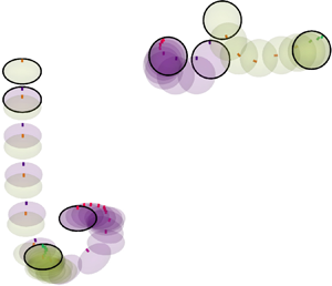
Single-particle regimes for heavy ( $\tilde {\rho }=1.5$) spheres and oblate spheroids with aspect ratio $\chi =1.5$ as a function of the Galileo number ${Ga}$. Reference data for dilute suspensions of spheres with the same density ratio and Galileo number from Uhlmann & Doychev (Reference Uhlmann and Doychev2014) are also included. The vortical flow structures in each regime are indicated with the aid of iso-surfaces of ${Q}$, the second invariant of the velocity gradient tensor (Hunt, Wray & Moin Reference Hunt, Wray and Moin1988).

Whenever the volume fraction ( $\varPhi$) of the particulate phase becomes non-negligible, particle–particle interactions can lead to significant collective effects. For dilute systems, these interactions are predominantly of indirect type, acting through long-range hydrodynamic forces. For denser systems, direct contacts between two or more particles come into play more frequently, thereby contributing to the exchange of momentum. In the present work we are interested in dilute systems (with solid volume fractions below one per cent), which is why we will concentrate on this regime in the following literature review. Depending on the values of the parameter triplet $(\varPhi,\tilde {\rho },{Ga})$, dilute suspensions can exhibit spatial particle distributions with significant non-homogeneity. A non-homogeneously distributed particle phase in turn is often accompanied by important macroscopic effects, such as an altered mean settling velocity and a modification of the induced fluid flow features.
At Galileo numbers of  ${O}(10)$ and density ratio $\tilde {\rho }=2$ it has been observed that dilute suspensions of spherical particles tend to form horizontally aligned pairs (Yin & Koch Reference Yin and Koch2008), while at larger Galileo numbers ( ${Ga}\approx 200$) and similar density ratios, where the wake flow features a significant recirculation region, a vertical alignment is more probable (Kajishima & Takiguchi Reference Kajishima and Takiguchi2002; Uhlmann & Doychev Reference Uhlmann and Doychev2014). Kajishima & Takiguchi (Reference Kajishima and Takiguchi2002) were the first to investigate the formation of large, columnar-shaped particle clusters due to wake effects. Their particle-resolved direct numerical simulations (PR-DNS) in triply periodic boxes showed that clusters tend to form for particle Reynolds numbers exceeding $200\ldots 300$ ( $Ga\approx 153\ldots 210$), leading to strongly enhanced average settling velocities. In their initial work, the particle rotation was suppressed for computational simplicity, and a density ratio $\tilde {\rho }=8.8$ was considered. In the follow-up work of Kajishima (Reference Kajishima2004), the effect of particle rotation was taken into account, and it was found that rotational motion leads to a lower concentration of particles in clusters, since particles tend to escape a cluster through a rotation-induced lift effect. Kajishima (Reference Kajishima2004) also determined a lower limit of the solid volume fraction for the occurrence of clustering. The PR-DNS of Uhlmann & Doychev (Reference Uhlmann and Doychev2014) were performed at a fixed density ratio $\tilde {\rho }=1.5$, and it was observed that columnar clusters do form for ${Ga}=178$ (which corresponds to an isolated particle in the steady oblique regime), while no clusters are formed at $Ga=121$ (steady vertical regime). The authors suggest that the onset of clustering in dilute suspensions of spherical particles is triggered by the bifurcation of the wake flow from steady axisymmetric to steady oblique, with the consequence that the particles in the latter case drift horizontally (with random azimuthal angle) leading to an enhanced probability of particle–particle encounters. Further data on collective effects upon clustering are available from the PR-DNS studies of Zaidi, Tsuji & Tanaka (Reference Zaidi, Tsuji and Tanaka2014), Fornari, Picano & Brandt (Reference Fornari, Picano and Brandt2016a) and Seyed-Ahmadi & Wachs (Reference Seyed-Ahmadi and Wachs2021), which were all performed in similar triply periodic configurations, and from the work of Huisman et al. (Reference Huisman, Barois, Bourgoin, Chouippe, Doychev, Huck, Morales, Uhlmann and Volk2016), who conducted experiments in a settling column with glass beads in water. An overview of the average settling velocities from these various datasets for dilute suspensions of spherical particles in an otherwise ambient fluid is given in figure 2. The PR-DNS results appear to give a consistent trend: for increasing values of the Galileo number the particles tend to settle at an average rate which is enhanced with respect to the velocity of an isolated particle, and there appears indeed to be a cross-over (from a reduced settling velocity to an enhancement) for $Ga\approx 150$. The limited available experimental data in this parameter range are not inconsistent with this picture, however, showing a settling enhancement already at lower Galileo number of $110$ and mild columnar cluster formation. Huisman et al. (Reference Huisman, Barois, Bourgoin, Chouippe, Doychev, Huck, Morales, Uhlmann and Volk2016) have identified the presence of the bounding container walls, which presumably causes a large-scale recirculating flow, as a possible cause for the observed discrepancy.
Mean settling velocity vs Galileo number for spherical and non-spherical suspensions of heavy particles with density ratio  ${O}(1)$ in the dilute regime. The velocity data are normalized with the corresponding mean settling velocity of an isolated particle in the asymptotic (long-time) limit. The error bars in the experimental data of Huisman et al. (Reference Huisman, Barois, Bourgoin, Chouippe, Doychev, Huck, Morales, Uhlmann and Volk2016) indicate minimum and maximum values of the repetitions performed by the authors. Present results are included for completeness.

Dilute suspensions of non-spherical particles have received much less attention, mainly due to the complexity associated with the particle shape and the corresponding increase in the size of the parametric space. Spheroids have been the preferred choice of several authors, partly due to their convenient parametrization. Their shape is defined uniquely by the aspect ratio  $\chi ={d}/ {a}$, where d and a are the equatorial diameter and the length of the symmetry axis, respectively (see figure 3a,b). The spheroidal shape allows for a smooth transition between flat, disk-like shapes (for very large values of $\chi$), and elongated, fibre-like geometries (for very small values of $\chi$), while a sphere is recovered for $\chi =1$. When oblate spheroids ( $\chi >1$) are considered, the regime maps of a single particle are more complex when compared with spheres (Zhou, Chrust & Dušek Reference Zhou, Chrust and Dušek2017). Despite this increase in complexity, specific combinations of $\chi$ and $\tilde {\rho }$ result in a single oblate spheroid exhibiting the so-called ‘sphere-like scenario’ in which the first bifurcation for increasing Ga is regular, transitioning from a vertical to an oblique regime (see figure 1, Zhou et al. Reference Zhou, Chrust and Dušek2017; Moriche, Uhlmann & Dušek Reference Moriche, Uhlmann and Dušek2021). Fornari, Ardekani & Brandt (Reference Fornari, Ardekani and Brandt2018) studied the settling of dilute suspensions of almost neutrally buoyant ( $\tilde {\rho }=1.02$) oblate spheroids with a moderately flat shape $\chi =3$. They considered both dilute and dense regimes at Galileo numbers at which a single particle follows a steady vertical path ( $Ga=60$) or an unsteady path which is vertical in the mean ( $Ga=140$). For their most dilute cases they observed a large enhancement of the mean settling velocity compared with the single-particle case, with only small differences between the two Galileo numbers (cf. figure 2). Fornari et al. (Reference Fornari, Ardekani and Brandt2018) have also detected non-homogeneous particle distributions in the form of vertical particle trains with lateral dimensions of the order of $10$ times the length of the symmetry axis, based upon visualization and on the analysis of pairwise distribution functions. The authors attributed the enhancement of settling velocity to the occurrence of particle-pair interactions which lead to the formation of piles of particles which practically stick to each other in the case of oblate spheroids with $\chi =3$.
View of the  $i$th spheroid in its body-fixed reference system (a) along the symmetry axis and (b) perpendicular to it. The blue line in (a,b) represents a sphere with the same volume. (c) Sketch of the problem in the global reference system.

Turning now to other shapes, Seyed-Ahmadi & Wachs (Reference Seyed-Ahmadi and Wachs2021) more recently studied the behaviour of settling cubes with  $\tilde {\rho }=2$, $\varPhi =0.01\ldots 0.2$ and Galileo numbers for which a single cube tends to a steady oblique path with very small tilting angle ( $Ga=70$) and to a helical path ( $Ga=160$) for large times. For their smallest solid volume fraction these authors report an increase in the relative settling velocity, which is similar to what is observed in suspensions of spheres (cf. figure 2). Interestingly, Seyed-Ahmadi & Wachs (Reference Seyed-Ahmadi and Wachs2021) observe that the intensity of columnar cluster formation (measured with the aid of particle-pair distribution functions) is somewhat lower in the case of cubes as compared with the spherical counterpart. This effect is attributed by the authors to higher rotation rates in the former case, leading to an enhanced lift force that increases their probability to escape from an existing cluster.
As noted above in the case of spheres, the settling regime of a single particle appears to be relevant to the macroscopic behaviour of dilute suspensions. As a next step towards the understanding of collective effects, it is useful to investigate the interaction of settling particle pairs, a set-up which may lead to the so-called drafting–kissing–tumbling (DKT) process (Fortes, Joseph & Lundgren Reference Fortes, Joseph and Lundgren1987). For sufficiently high Galileo number, a trailing sphere initially released inside of the wake region of a leading sphere will approach the latter one during the drafting phase, they will touch (‘kissing’), and then interchange positions (‘tumbling’), since a vertically aligned pair of spheres is unstable, before eventually separating. The reduced size of the problem compared with the many-particle cases makes (DKT) simulations a useful laboratory to understand the underlying physics of many-particle cases. Indeed, Fortes et al. (Reference Fortes, Joseph and Lundgren1987) used auxiliary cases with the DKT set-up to support their results on the spatial structure of many spherical particles in a fluidized bed. Regarding non-spherical particles, Ardekani et al. (Reference Ardekani, Costa, Breugem and Brandt2016) observed a suppression of the tumbling phase in pairwise interactions of moderately flat oblate spheroids ( $\chi =3$), as well as an increased collision domain. The authors conjectured that the essentially infinite interaction time of piled up particles would lead to enhanced clustering in the corresponding many-particle case. This conjecture was later indeed confirmed by Fornari et al. (Reference Fornari, Ardekani and Brandt2018).
The numerical simulations of DKT cases in the literature use a common configuration: two particles settling in an initially quiescent fluid inside a container, whose vertical size should be large enough to accommodate the different stages of the DKT case, and also minimize the (undesired) influence of the lower boundary of the computational domain. The vertical size of the container varies from  $20D$ (Glowinski et al. Reference Glowinski, Pan, Hesla, Joseph and Périaux2001; Breugem Reference Breugem2012) to approximately $40D$ (Patankar et al. Reference Patankar, Singh, Joseph, Glowinski and Pan2000; Ardekani et al. Reference Ardekani, Costa, Breugem and Brandt2016). The main drawback of this configuration is that any modification of the parameters (for example the relative initial position between the particles) which increases the duration of the drafting phase, would require a further increase of the computational domain. As a result, the simplicity of the DKT set-up is somehow diminished. Using periodic boundary conditions in the vertical direction, as some authors have done for single-particle cases (Kajishima & Takiguchi Reference Kajishima and Takiguchi2002; Doychev Reference Doychev2014), also demands large domains in order to minimize wake effects from periodic repetitions. To overcome these difficulties, in the present work we propose to use inflow/outflow boundary conditions along the vertical direction along with a carefully adjusted vertical velocity at the inflow. Thus, the settling particles are not perturbed by their own wakes, and the domain size becomes less of a critical parameter. To the best of our knowledge, this strategy has not been employed previously. Here, it allows us to employ moderately small computational domains, so that we can perform a campaign of simulations varying the relative initial position of the particle pair and, therefore, we can obtain statistically significant results.
In the present work we analyse the clustering behaviour of dilute suspensions of spheroids with a relatively low aspect ratio  $\chi =1.5$, a density ratio $\tilde {\rho }=1.5$ and two Galileo numbers $Ga=\{111, 152\}$. For these spheroids a single particle exhibits the so-called ‘sphere-like scenario’ (Zhou et al. Reference Zhou, Chrust and Dušek2017), and for suitable initial conditions a pair of them undergo the three stages in a pairwise interaction (DKT). Our aim is to explore collective effects for non-spherical particle shapes, while remaining relatively close to the well-explored spherical shape. The overarching question is: How do relatively small deviations from the spherical shape affect the settling behaviour of a dilute suspension of rigid particles? In addition to many-particle simulations in large domains, we perform a large set of DKT simulations of the mentioned spheroids as well as for the reference case with spheres in which we analyse the effect of particle shape and of the angular motion by either suppressing or allowing the latter.
The manuscript is structured as follows: in § 2 we present the mathematical model describing the settling of particles in unbounded, otherwise quiescent fluid and, in § 3 we specify the numerical method and the physical and numerical parameters. Results are presented in two steps: in § 4.1 we focus on many-particle cases, which represent the core of this work, and in § 4.2 we analyse a set of auxiliary simulations of a DKT configuration in order to support the observations made in the many-particle cases. In § 5 we discuss the implications of the DKT results for the many-particle case. Finally, a summary and conclusions can be found in § 6.
2. Problem description
We study the settling of particles under the action of gravity in an unbounded, initially quiescent fluid. We consider an incompressible Newtonian fluid of density  $\rho _{f}$ and kinematic viscosity $\nu$. Particles are oblate spheroids of equatorial diameter d and aspect ratio $\chi ={d}/a$, where a is the length of their symmetry axis (see figure 3a,b). The particles are assumed to be rigid with homogeneous mass density $\rho _{p}$, which is larger than that of the fluid ( $\rho _{p}>\rho _{f}$). The gravitational acceleration $\boldsymbol {g}$ points in the negative $z$-direction, $\boldsymbol {g} = -g\boldsymbol {e}_{z}$, where ${g}$ is the modulus of the gravitational acceleration (see figure 3c).
The fluid velocity  $\boldsymbol {u}=({u},v,w)$ is governed by the Navier–Stokes equations for an incompressible, constant density fluid
 $$\begin{gather} \frac{\partial \boldsymbol{u}}{\partial t}+\left(\boldsymbol{u}\boldsymbol{\cdot}\boldsymbol{\nabla}\right)\boldsymbol{u} ={-}\frac{\boldsymbol{\nabla} p}{\rho_{f}} +\nu \nabla^2\boldsymbol{u}, \end{gather}$$
 $$\begin{gather}\boldsymbol{\nabla}\boldsymbol{\cdot}\boldsymbol{u}=0 , \end{gather}$$
where  $p$ is the pressure. No-slip and no-penetration boundary conditions are imposed on the surface of each particle. The linear and angular velocities of the particles, $\boldsymbol {u}_{p}=(u_{p},v_{p},w_{p})$ and $\boldsymbol {\omega }_p=(\omega _{px},\omega _{py},\omega _{pz})$, respectively, are governed by the Newton–Euler equations
 $$\begin{gather} V_p\rho_p \frac{{\rm d}\boldsymbol{u}_p}{{\rm d}t}=\int_{S} \boldsymbol{\tau}\boldsymbol{\cdot}\boldsymbol{n} \, \text{d} \sigma +\left(\rho_{p}-\rho_{f}\right)V_p\boldsymbol{g} + \boldsymbol{F}, \end{gather}$$
 $$\begin{gather}\frac{{\rm d}\left({\boldsymbol{I}_{p}}\boldsymbol{\omega}_{p}\right)}{{\rm d}t}= \int_{S} \boldsymbol{r}\times \left(\boldsymbol{\tau}\boldsymbol{\cdot}\boldsymbol{n}\right) \text{d} \sigma + \boldsymbol{T}, \end{gather}$$
where  $V_{p}$ and $S$ are the volume and the surface of the particle, respectively, $\boldsymbol {n}$ is a unit vector normal to $S$ pointing towards the fluid, $\boldsymbol {\tau }$ is the stress tensor ( $\boldsymbol {\tau }=-pI+\rho _{f}\nu (\boldsymbol {\nabla }\boldsymbol {u}+\boldsymbol {\nabla }\boldsymbol {u}^T)$), $\boldsymbol {r}$ is a position vector with respect to the centre of gravity of the particle and $\boldsymbol {F}$ and $\boldsymbol {T}$ are the solid–solid contact force and torque, respectively.
The problem is governed by four non-dimensional parameters, namely the density ratio between the particles and the fluid,  $\tilde {\rho }=\rho _{p}/ \rho _{f}$, the aspect ratio of the particles, $\chi$, the Galileo number, Ga, and the solid volume fraction, $\varPhi$. The solid volume fraction is defined as $\varPhi =\varSigma _p/( \varSigma _p+\varSigma _f)$ where $\varSigma _p$ and $\varSigma _{f}$ represent the volume occupied by the particles and the fluid, respectively.
In this work we are interested in the dilute regime, and we set the solid volume fraction to  $\varPhi =5\times 10^{-3}$. Regarding the shape of the particles, we select oblate spheroids of aspect ratio $\chi =1.5$, which is a moderately small deviation from the spherical reference geometry, that in turn has been extensively investigated in the past. In particular, it is known that the settling regime map for oblate spheroids with $\chi =1.5$ resembles that of a sphere (Moriche et al. Reference Moriche, Uhlmann and Dušek2021). We fix the density ratio at $\tilde {\rho }=1.5$ (which corresponds e.g. to some plastic materials in water), and we select two values of the Galileo number: one for which a single particle follows a steady vertical path ( $Ga=110.56$), and another which leads to a single particle following a steady oblique path ( $Ga=152.02$).
2.1. Definitions
A velocity scale based on the gravitational acceleration, the density ratio and the size of the particle can be defined as follows:
 \begin{equation} U_{g}=\sqrt{\left|\tilde{\rho}-1\right|{g}D}, \end{equation}
where  $D=d\chi ^{-1/3}$ is the diameter of a sphere with the same volume as the spheroid considered. Based on the velocity scale $U_{g}$ (2.3) the Galileo number is defined as
 \begin{equation} Ga=\frac{U_{g}D}{\nu} , \end{equation}
and an a priori gravitational time scale can be formed as follows:  $\tau _{g}=D/U_{g}$. For future reference let us define the relative velocity $\boldsymbol {u}_{pr}^{(i)}=( u_{pr}^{(i)},v_{pr}^{(i)},w_{pr}^{(i)})$ of the $i$th particle with respect to the mean fluid velocity as
 \begin{equation} \boldsymbol{u}_{pr}^{(i)}(t)=\boldsymbol{u}_{p}^{(i)}(t)-\langle \boldsymbol{u}\rangle_f(t), \end{equation}
where the average operator  $\langle {\cdot } \rangle _f$ indicates spatial averaging over the entire domain occupied by the fluid $\varOmega _f$, viz.
 \begin{equation} \langle {\cdot} \rangle_f =\frac{1}{\varSigma_f} \int_{\varOmega_f} \left({\cdot} \right)\text{d} {\boldsymbol{x}}. \end{equation}
Let us also introduce the time-dependent settling velocity, averaged over the set of particles as
 \begin{equation} w_{s}(t) = \langle w_{pr}\rangle_p(t) , \end{equation}
where the average operator  $\langle {\cdot } \rangle _p$ indicates the ensemble average over the dispersed phase, which for a set of $N_{p}$ particles is expressed as
 \begin{equation} \langle {\cdot} \rangle_p = \frac{\displaystyle \sum_{i=1}^{{N_{p}}} \left({\cdot}\right)^{(i)}}{ N_{p}}. \end{equation}
Similarly, the standard deviation of the vertical and horizontal components of the linear and angular particle velocity are defined as
 $$\begin{gather} w_s^{std}(t) =\langle w_{pr}^{\prime (i)}w_{pr}^{\prime (i)}\rangle_p^{1/2}, \end{gather}$$
 $$\begin{gather}u_h^{std}(t) =((\langle u_{pr}^{\prime (i)}u_{pr}^{\prime (i)}\rangle_p+ \langle v_{pr}^{\prime (i)}v_{pr}^{\prime (i)}\rangle_p)/2)^{(1/2)}, \end{gather}$$
 $$\begin{gather}\omega_{v}^{std}(t) =\langle \omega_{pz}^{\prime (i)}\omega_{pz}^{\prime (i)}\rangle_{p}^{1/2}, \end{gather}$$
 $$\begin{gather}\omega_{h}^{std}(t) =((\langle\omega_{px}^{\prime (i)} \omega_{px}^{\prime (i)}\rangle_p+ \langle\omega_{py}^{\prime (i)}\omega_{py}^{\prime (i)}\rangle_p)/2)^{(1/2)}, \end{gather}$$
where the prime symbol indicates that the quantity is the fluctuating part of the variable, defined as
 \begin{equation} \left({\cdot}\right)' = \left({\cdot}\right) - \langle {\cdot} \rangle. \end{equation}
Finally, it should be mentioned that the definition of the Galileo number used in this work is equivalent to that used in Fornari et al. (Reference Fornari, Picano, Sardina and Brandt2016b) and Ardekani et al. (Reference Ardekani, Costa, Breugem and Brandt2016) for spheroids, and to that of Seyed-Ahmadi & Wachs (Reference Seyed-Ahmadi and Wachs2021) for cubes. We have selected this definition over the one used in some works dealing exclusively with spheroids (Zhou et al. Reference Zhou, Chrust and Dušek2017; Moriche et al. Reference Moriche, Uhlmann and Dušek2021) in order to recover the same value of Ga when working with spheres ( $\chi =1$).
For a multiparticle case with a given parameter pair ( $Ga,\tilde {\rho })$, independently of its solid volume fraction $\varPhi$, we define the reference velocity ${w_{ref}}$ as
 \begin{equation} {w_{ref}}\left({Ga},\tilde{\rho}\right) = \left| w_{pr}\right| , \end{equation}
where the value of  $w_{pr}$ in (2.11) is taken from the corresponding single-particle case. Please note that, for the cases considered here, the single-particle case regime is steady, therefore no (temporal or statistical) averaging is needed to compute $w_{ref}$ in (2.11).
According to the above definitions of  $w_{s}$ and $w_{ref}$, we define the average particle Reynolds number
 \begin{equation} Re_{D}=\frac{\left|\langle \omega_s\rangle_t\right|D}{\nu} , \end{equation}
and the single-particle Reynolds number
 \begin{equation} Re_D^0=\frac{w_{ref}D}{\nu} , \end{equation}
where the operator  $\langle {\cdot } \rangle _t$ indicates temporal averaging.
3. Methodology
3.1. Numerical method
The Navier–Stokes equations (2.1) are integrated in time by means of a three-stage Runge–Kutta scheme in which the viscous term is treated implicitly and the advective term explicitly (Rai & Moin Reference Rai and Moin1991; Verzicco & Orlandi Reference Verzicco and Orlandi1996). The fractional step method proposed by Brown, Cortez & Minion (Reference Brown, Cortez and Minion2001) is used to fulfil the continuity constraint. Spatial derivatives are approximated with central finite differences of second order on a staggered, uniform, Cartesian grid.
The presence of the body is modelled by the direct-forcing immersed boundary method proposed by Uhlmann (Reference Uhlmann2005) and later extended to track the motion of non-spherical particles by Moriche et al. (Reference Moriche, Uhlmann and Dušek2021), where extensive validation of the method can be found. Collisions are modelled with a repulsive short-range normal force (with a range  $\Delta x$) so as to avoid non-physical overlapping of particles (details can be found in Appendix A).
In a triply periodic set-up, gravity continuously accelerates the system. Therefore, in order to allow for a steady state, we add a constant-in-space source term to the vertical momentum equation whose volume integral is equal (and opposite in sign) to the net force exerted by the particles on the fluid (Höfler & Schwarzer Reference Höfler and Schwarzer2000).
3.2. Computational set-up
The computational domain is a cuboid with triply periodic boundary conditions, whose size is the result of a compromise between computational resource requirements and physical realism. Based on preliminary tests we choose a domain size of approximately  $55D$ in the lateral directions and approximately $220D$ in the vertical direction. Please note that a full decorrelation in the vertical direction is not warranted once clustering sets in, and in the horizontal direction once the clusters grow to a size comparable to the computational domain. This lack of full decorrelation, which was also observed in the case of corresponding spheres (Doychev Reference Doychev2014), is further discussed in Appendix B. We select a spatial resolution of $D/\Delta x\approx 21$ ( ${d}/ \Delta x=24$), which is supported by the work of Moriche et al. (Reference Moriche, Uhlmann and Dušek2021). In their work the authors show that, compared with a spectral/spectral-element solution, the error in the mean settling velocity of a single spheroid of aspect ratio $\chi =1.5$, density ratio $\tilde {\rho }=2.14$ at $Ga=152.02$ is smaller than $2\,\%$. In the present case this results in a grid of $[1152 \times 1152 \times 4608]$ points. Table 1 shows the parameters of the two simulations presented in this work.
Parameters of the present cases and of those in Uhlmann & Doychev (Reference Uhlmann and Doychev2014).

3.3. Initialization
In order to initialize the flow around the particles we simulate an initial transient during a time interval of  $66.67D/\langle w\rangle _{f}$ in which the particles are fixed. The initial position of the particles follows a random uniform distribution. Their orientation is randomly distributed with a maximum deviation of ${\pm }5^\circ$ tilting angle with respect to the vertical axis. The objective of constraining the angular position is to obtain a slight perturbation of the angular position with respect to the stable position of settling spheroids at moderate Ga. The same initial distribution of particles is used in both cases presented in table 1.
During the fixed-particle transient we impose the Reynolds number of the flow relative to the particles,  $Re_{D}^{0}$, as obtained (as an output parameter) in the simulations with an isolated mobile particle at the target value of the respective Galileo number, cf. table 2. This is realized by means of a constant vertical pressure gradient, similar to the body force which counteracts the acceleration of the system when particles are freely mobile (Uhlmann & Doychev Reference Uhlmann and Doychev2014). As will be shown later, the flow around the particles during the initial fixed-particle transient mostly resembles that of the analogous single-particle case at the given $Re_{D}^{0}$, due to the low concentration of particles in both cases. It should be mentioned that during this initial transient we obtain good decorrelation of all flow velocity components in all spatial directions (see Appendix B). Once the particles are released, the mean fluid flow relative to the particles is maintained through the above mentioned body force. Therefore, if perfectly adjusted, a single particle would not exhibit any vertical motion in the computational reference system, while the vertical motion of the many-particle ensemble is entirely due to mutual interactions (Uhlmann & Doychev Reference Uhlmann and Doychev2014).
Single-particle regime and time-averaged results of the present cases and those in the work of Uhlmann & Doychev (Reference Uhlmann and Doychev2014).

4. Results
In this section we present the results obtained for many-particle cases after particles are released. We also present additional simulations of settling particle pairs in order to analyse their ‘DKT’ dynamics.
4.1. Clustering phenomena in many-particle cases
When particles are released, they start to interact with their neighbours by repeated DKT events. The interaction between particles is intense in both cases G111 and G152, and rather similar (see animations in the supplementary material). In the following we present: (i) the enhanced settling and quantification of clustering, (ii) the angular motion of the particles, (iii) the arrangement of particles’ trajectories and (iv) a visualization of the main features of the flow.
4.1.1. Enhanced settling and quantification of clustering
Figure 4(a) shows the time history of the average particle settling velocity defined in (2.9). It can be seen that, in both present cases, the ensemble of mildly oblate spheroids reaches on average a much enhanced settling velocity magnitude after an initial transient of approximately  $400\tau _{g}$, after which the values saturate and continue fluctuating around a value of roughly $-1.25$. This behaviour is quite in contrast to the known results for spheres (also included in the figure for reference) for which a transition from expected settling to enhanced settling occurs in the corresponding range of Galileo numbers, and for which the enhancement of the settling velocity was found to be less pronounced (only roughly half of the present increase). Instead, the present suspension of spheroids with $\chi =1.5$ appears to behave qualitatively similar to the much more flattened ( $\chi =3$), almost neutrally buoyant ( $\tilde {\rho }=1.02$) spheroids of Fornari et al. (Reference Fornari, Ardekani and Brandt2018), for which the magnitude of the mean collective settling velocity was found to increase by over $30$ %.
Time history of (a) enhancement of the settling velocity ( $w_s$), and standard deviation of (c) settling and (d) horizontal velocity, normalized with the reference settling velocity from the single-particle counterpart ( $w_{ref}$). (b) Temporal evolution of the standard deviation of Voronoï cell volumes ( $\langle \tilde {V}_i^{\prime }\tilde {V}_{i}^{\prime }\rangle ^{1/2}$), normalized with the value obtained for a random Poisson process ( $\langle \tilde {V}_i^{\prime }\tilde {V}_{i}^{\prime }\rangle _{rnd}^{1/2}$). Reference data for spheres are from Uhlmann & Doychev (Reference Uhlmann and Doychev2014).

For completeness, let us report that the amplitude of the particle velocity fluctuations (cf. figure 4c,d) follows a similar trend as the mean settling velocity, with a nearly linear growth during the initial transient and subsequent fluctuations around time-averaged values of approximately  $w_s^{std} \approx 0.4w_{ref}$, $u_{h}^{std} \approx 0.2w_{ref}$. It should be noted that a clear signature of the oblique motion of individual particles just after their release is visible in case G152, as can be seen in terms of an initial peak of the intensity of the horizontal particle motion visible in the inset in figure 4(d). After approximately $10\tau _{g}$ this peak disappears, and the two suspensions of spheroids at different Galileo numbers exhibit very similar temporal evolutions.
In order to investigate the spatial structure of the disperse phase, we make use of the normalized Voronoï cell volume
 \begin{equation} \tilde{V}_i = \frac{V_v^{(i)}}{\langle V_v\rangle_p}, \end{equation}
where  $V_{v}^{(i)}$ is the volume of the $i$th cell of the Voronoï diagram obtained from a three-dimensional tessellation of space based on the centroid locations of the particles (Monchaux, Bourgoin & Cartellier Reference Monchaux, Bourgoin and Cartellier2012; Uhlmann & Doychev Reference Uhlmann and Doychev2014). In order to quantify the tendency to cluster we compare the standard deviation of $\tilde {V}_i$ with the same quantity obtained in a random Poisson process (RPP) of particles with the same shape and with the same solid volume fraction. For a mean concentration of particles such that $\varPhi =5\times 10^{-3}$, these RPP reference values are $\langle \tilde {V}_{i}^{\prime }\tilde {V}_{i}^{\prime }\rangle _{rnd}^{1/2}=0.4176$ for oblate spheroids of $\chi =1.5$ (determined in the framework of the present work) and $\langle \tilde {V}_{i}^{\prime }\tilde {V}_{i}^{\prime }\rangle _{rnd}^{1/2}=0.4146$ for spheres (given in Uhlmann Reference Uhlmann2020). The graph in figure 4(b) shows the temporal evolution of the standard deviation of the Voronoï cell volumes, normalized with the reference value from RPP. A direct qualitative correspondence with the temporal evolution of the (magnitude of the) mean settling velocity in figure 4(a) can be observed. More specifically, after a similar initial transient with an approximately linear growth of $\langle \tilde {V}_{i}^{\prime }\tilde {V}_{i}^{\prime }\rangle ^{1/2}$, the present suspensions of spheroids at both Galileo number values reach very large clustering intensities, which by far exceed those reported for spheres (cf. case M178 from Uhlmann & Doychev Reference Uhlmann and Doychev2014). Based on the previous knowledge for settling spheres, and on the fact that the present spheroids with $\chi =1.5$ are not too far from a spherical shape, the strong clustering of the lower Galileo number case G111 is unexpected.
Next, we present time-averaged data of some of the time-dependent quantities discussed above. We discard the initial transient, and we start collecting statistics at  $t=500\tau _{g}$, resulting in a sampling time interval of approximately $1000\tau _{g}$. Figure 5(a) shows the time-averaged values of $\langle \tilde {V}_{i}^{\prime }\tilde {V}_{i}^{\prime }\rangle ^{1/2}$ plotted vs the Galileo number. It can be clearly seen that the present suspensions of spheroids feature strong clustering with little effect of varying the value of the Galileo number. Interestingly, it turns out that the magnitude of the mean settling velocity normalized by the single-particle reference value is approximately proportional to the standard deviation of the Voronoï cell volumes normalized by its random value, i.e. to the clustering intensity. This relation is shown in figure 5(b), for the present spheroids and for the sphere suspensions of Uhlmann & Doychev (Reference Uhlmann and Doychev2014) and of Doychev (Reference Doychev2014). This observation should be checked with the help of additional datasets in the future, since – if confirmed – it might open up a possibility to determine the mean settling velocity of a collective from knowledge on the spatial structure of the dispersed phase alone.
(a) Time-averaged values of the standard deviation of Voronoï cell volumes,  $\langle \tilde {V}_{i}^{\prime }\tilde {V}_{i}^{\prime }\rangle _t^{1/2}$, normalized with the RPP reference values vs Ga. (b) Magnitude of the time-averaged mean settling velocity, $w_s$, vs $\langle \tilde {V}_{i}^{\prime }\tilde {V}_{i}^{\prime }\rangle _t^{1/2}$. Reference data for spheres from Uhlmann & Doychev (Reference Uhlmann and Doychev2014) and Doychev (Reference Doychev2014).

The distinct spatial arrangement of the spheroids compared with spheres can be further characterized with the aid of the probability density functions (p.d.f.s) of the normalized Voronoï cell volumes  $\tilde {V}$. Figure 6 shows the p.d.f. of $\tilde {V}$ of both cases with spheroids (G111 and G152) together with the p.d.f. of a RPP (Uhlmann Reference Uhlmann2020) and the p.d.f.s of two cases with spheres taken from Uhlmann & Doychev (Reference Uhlmann and Doychev2014) (their cases M121 and M178). The same qualitative behaviour is observed in both cases with spheroids: the probability of finding volumes smaller than the average ( $\tilde {V}=1$) is high compared with a RPP. This indicates that most of the particles form part of clusters. Similarly, the probability of finding large volumes ( $\tilde {V}\gtrsim 2$) is higher than that of a RPP, which implies the presence of particles in large void regions. Contrarily, case M121 from Uhlmann & Doychev (Reference Uhlmann and Doychev2014) shows a tendency to a more ordered state, where the probability of finding volumes similar to the average value is higher.
Probability density function of the normalized Voronoï cell volumes in (a) linear and (b) logarithmic scale. Reference data for spheres are from Uhlmann & Doychev (Reference Uhlmann and Doychev2014).

4.1.2. Angular velocity and orientation of particles
Figure 7(a) shows the time history of the standard deviations of the horizontal and vertical components of the angular velocity of the particles normalized with  $w_{ref}/D$. Figure 7(b) shows the time history of the averaged and standard deviation of the tilting angle $\varphi _{v}$, which is defined as the angle between the symmetry axis of the spheroid and the vertical direction ( $0\leq \varphi _{v}\leq 90^\circ$). The time evolution of these four quantities is remarkably different from the time evolution of the quantities reported in figure 4. Within a few gravitational time units after the particle release all quantities in figure 4 increase from zero to values close to their asymptotic time averages, after which they vary only very mildly. This indicates that the angular motion of the particles shows less sensitivity to collective effects than does the linear motion. Note that the converged values are slightly higher in case G152 when compared with case G111, except for $\langle \varphi _{v}^{\prime }\varphi _{v}^{\prime }\rangle _{p}^{1/2}$, that presents values which are approximately equal in both cases.
Time history of (a) standard deviation of the angular velocity and (b) average and standard deviation of the orientation angle  $\varphi _{v}$.

Now let us focus on the p.d.f. of these angular quantities. Figure 8 shows the p.d.f. of the vertical and horizontal components of the angular velocity. We have tried several known p.d.f.s and we found Laplace's distribution
 \begin{equation} f\left(x;\beta\right) = \left(2\beta\right)^{{-}1}\exp\left(\left|x\right|/\beta\right), \end{equation}
with  $\beta$ being a free parameter (cf. fitted numerical values in the figure), the best fit to both components of the angular velocity. This highlights the exponential tails, i.e. the importance of extreme events of the angular particle motion. The vertical component shows, however, an approximately $20\,\%$ smaller value for $\beta$ than the horizontal counterpart, indicating a more localized distribution with higher kurtosis. Similarly, we found the best fit of the estimated p.d.f. of the tilting angle $\varphi _{v}$ with respect to the vertical to be a gamma distribution
 \begin{equation} f\left(x;k,\theta\right) = \frac{x^{k-1}}{\theta^k\varGamma(k)}\exp\left({-}x/\theta\right) , \end{equation}
where  $k$ and $\theta$ are the shape and scale parameters. Figure 9(a) shows the p.d.f. of $\varphi _{v}$ and the fitted Gamma distribution. The obtained fitting shows very good agreement in the range $0^\circ <\varphi _{v}\lesssim 30^\circ$. For higher values $\varphi _v>30^\circ$, the p.d.f. of each case shows a lower decay rate compared with the fitted gamma distribution for both cases. The shape parameter of the fitted gamma distribution in both cases ( $k\approx 2.3$) indicates a fast, but non-abrupt approach to zero of the p.d.f. in the limit $\varphi _{v}\rightarrow 0^+$. Please recall that, from the shape parameter of the gamma distribution, we can infer the following: when $k\leq 1$ the maximum probability is located at $\varphi _{v}=0$ and then the p.d.f. decreases monotonically as $\varphi _{v}$ increases, when $k>1$ the limit of the p.d.f. as $\varphi _{v}\rightarrow 0^+$ is zero (with strong gradients in the vicinity of $\varphi _{v}=0$ for values of $k$ closer to unity), and when $k\geq 3$ the distribution shows a slow increase of the probability in the vicinity of zero (see figure 9b). Finally, the non-intuitive zero value of the p.d.f. in the limit $\varphi _{v}\rightarrow 0^+$ can be explained by the circumferential shape of the bins used to generate it. In order to obtain the p.d.f. for a specific value of ${\varphi _{v}}_0$, we define a bin by its edges $[{\varphi _{v}}_a,{\varphi _{v}}_b]$, where ${\varphi _{v}}_a < {\varphi _{v}}_0 < {\varphi _{v}}_b$. In the limit $\varphi _{v}\rightarrow 0^+$ and for increasing resolution of the p.d.f. ( ${\varphi _{v}}_b - {\varphi _{v}}_a\rightarrow 0$), the area on the surface of a sphere between the edges tends to zero, and as a consequence the probability of finding occurrences of $\varphi _{v}$ such that ${\varphi _{v}}_a < \varphi _{v} < {\varphi _{v}}_b$, also tends to zero.
Probability density functions of the (a) vertical and (b) horizontal components of the angular velocity. The curves are fitted to a Laplace distribution whose parameter  $\beta$ is indicated in the legend. The Gaussian curve is shown for comparison purposes.

(a) The p.d.f. of the tilting angle  $\varphi _{v}$ of cases G111 and G152 (the same information with the $y$ axis in logarithmic scale is shown in (b). A fitted gamma distribution is included (parameters from fitting included in the legend).

4.1.3. Trajectories
Now we turn our attention to the trajectories of the particles. Figures 10, 11 and 12 show the trajectories followed by the centre of gravity of the particles during a time span of  $0.54\tau _{g}$ leading up to three successive time instants in two perpendicular projections. With this representation, considering the initialization procedure (§ 3.3) and if, hypothetically, collective effects were absent, particles would be represented by single points in the case G111 (single particle follows steady vertical trajectory) and by straight horizontal lines in the case G152 (single particle follows steady oblique trajectory). The time instants selected are $t/\tau _{g}\approx 10\,400$ and $1500$, which correspond to: (i) shortly after the particles are released, (ii) the end of the linear growth of $w_s$ and $\langle \tilde {V}_{i}^{\prime }\tilde {V}_{i}^{\prime }\rangle ^{1/2}$ (see figure 4) and (iii) the asymptotic state close to the end of the simulated time, respectively. Shortly after particles are released ( $t/\tau _{g}\approx 10$), there is almost negligible motion of the particles in case G111 (figures 10(a) and 11(a) show point-like trajectories) and a small lateral motion in case G152 (figures 10(b) and 12(a) show trajectories with a noticeable horizontal component). As both cases evolve, the trajectories show elongated shapes along the vertical direction, indicating an enhancement of the settling velocity compared with the single-particle configuration. On average, the length of the trajectories in the vertical direction keeps growing during the constant acceleration phase ( $t\lesssim 400\tau _{g}$) forming columnar clusters whose size is comparable to that of the computational domain (figures 10c and 10d, 11b and 12b). Again, the similarity of both cases is clearly noticeable. There is, however, a tendency of the clusters in the case of lower Galileo number to be more stable compared with the case of higher Galileo number when $t\approx 400\tau _{g}$ (see figures 11b and 12b). We believe that the smaller flow disturbances of the low Galileo number case allow the presence of clusters with a cross-section of the order of tens of $D$ (see figure 10c) to fill the entire domain in the vertical direction, whereas clusters of the same size in the horizontal direction of the higher Galileo number case (see figure 10d) are not stable and thus, appear to be more localized. This could explain the higher enhancement of the settling velocity with respect to the single particle case observed in the case at lower Galileo number (figure 4a) but it should be noted that this is only possible due to the periodic configuration. Therefore, the larger enhancement in $w_s$ observed in figure 4(a) for case G111 should be interpreted with care. In the horizontal direction, clusters show a continuous growth until they reach a size comparable to the computational domain (figure 10e, f).
Top view of trajectories of the particles’ centre of gravity during a time span of  $[t_0-T_t,t_0]$, where $T_t=0.54\tau _{g}$ for cases G111 (a,c,e) G152 (b,d, f). Trajectories are coloured according to the particle's velocity relative to the mean velocity of the mixture (red downwards, blue upwards).

As in 10 but for case G111 only and viewed from the side.

As in 10 but for case G152 only and viewed from the side.

4.1.4. Flow visualization
Figure 13 shows visualizations of the cases G111 and G152 just before releasing the particles (panels a,b,e, f) and two converged states (panels c,d,g,h). In the figure the particles are represented together with isocontours of the second invariant (Q) of the velocity gradient tensor (Hunt et al. Reference Hunt, Wray and Moin1988) and isocontours of the filtered vertical velocity  $\tilde {w}$. The filter applied to ${w}$ is a Gaussian filter of width $2.3D$ used to visualize large-scale velocity fluctuations. Just before particles are released ( $t/\tau _{g}=0$) we observe that in case G111 ( $Re_{D}^{0}=105$) the most common flow structure is a toroidal vortex around each particle (figure 13e), whereas in case G152 ( $Re_{D}^{0}=158$) we also frequently observe a double-threaded wake (figure 13f). The similarity of these vortical structures with the analogous single-particle case at the given $Re_{D}^{0}$ is due to the low concentration of particles in both cases. After convergence has been reached ( $t/\tau _{g}>1000$) both cases show large regions of high-speed downward flow, which are absent when particles are released ( $t=0$). The strong clustering of both cases discussed above is clearly seen when comparing the initial and converged snapshots of both cases.
Visualization of isocontours of  $QD^2/U_{g}^2=0.7$ (case G111) and $0.83$ (case G152) and $\tilde {w}=\langle w\rangle _f-0.5U_{g}$. Particles are represented in pink, isocontours of $Q$ with grey-coloured surfaces and isocontours of $\tilde {w}$ with yellow surfaces. (a–d) Show the whole domain ( $Q$ and $\tilde {w}$), (e–h) show a part of the domain (only Q). First and second columns correspond to the instant before the release of the particles of cases G111 and G152, respectively. Third and fourth columns correspond to a converged state of each case.

4.2. Drafting–kissing–tumbling
Since animations show that interactions between particle pairs occur frequently in the many-particle cases, we now proceed to an analysis of the interaction of such pairs in isolation. As we will see, these interactions are quite sensitive to the particle shape, and we believe that pairwise interactions are the key to understanding the tendency of oblate spheroids to cluster at Galileo numbers for which spheres do not exhibit clustering. We restrict the analysis to one combination of Galileo number and density ratio ( $Ga=111$, $\tilde {\rho }=1.5$) for which a single spheroid of aspect ratio $\chi =1.5$ and a single sphere result in a steady vertical regime (Jenny et al. Reference Jenny, Dušek and Bouchet2004; Moriche et al. Reference Moriche, Uhlmann and Dušek2021). As mentioned above, many-particle cases in the dilute regime ( $\varPhi = 5\times 10^{-3}$) with this combination of Ga and $\tilde {\rho }$ present strong clustering in the case of oblate spheroids with $\chi =1.5$ and no clustering in the case of spheres (Uhlmann & Doychev Reference Uhlmann and Doychev2014). We include an additional series in this set of DKT cases, in which the angular motion is suppressed. Therefore, we have these four configurations:
(i) Free-to-rotate spheres (angular motion enabled).
(ii) Rotationally locked spheres (angular motion suppressed).
(iii) Free-to-rotate spheroids (angular motion enabled).
(iv) Rotationally locked spheroids (angular motion suppressed).
This is motivated by the study of Kajishima (Reference Kajishima2004) who demonstrated that suppressing the rotation of spheres leads to an enhanced clustering tendency. We perform a parametric sweep of  $72$ initial relative particle positions for each configuration, resulting in a total number of $288$ simulations (see figure 14i). The problem set-up is analogous to the set-up of the many-particle cases presented in § 3, except that only two particles are present, and that we use an inflow/outflow configuration in the vertical direction as described in detail in Appendix C.
Trajectories of the trailing and leading particles for selected initial positions of spheres (a–d) and spheroids with  $\chi =1.5$ (e–h), all with $\tilde {\rho }=1.5$ at $Ga=111$. The reference frame is translating downwards at a constant speed slightly smaller than the settling velocity of a single particle ( $0.975w_{ref}$). Each panel contains the data of the cases with angular motion enabled and suppressed for a single initial condition and particle shape (see legend). (i) A sketch of the problem and the coordinates used is presented, in which the leading particle is represented with its actual shape and the trailing particle with a marker. The point markers correspond to all the initial conditions which we have computed, and the symbol markers to those initial conditions which are shown in panels a–h. (j) Sketch of the $x',y'$ coordinates.

Figure 14 shows the trajectories of  $16$ selected cases projected onto a vertical plane intersecting the particles at their initial position. These cases correspond to different initial conditions of the four selected configurations. Please note that in these four cases particles do collide at least once, while this is not the case for all initial separations (as will be shown in figure 16 below). If we focus on the trajectories of the trailing particles, there is a clear similarity in free-to-rotate and rotationally locked spheroids: for these two configurations the trailing particle of the four initial conditions shown in the figure moves laterally until its centre is vertically aligned with the leading particle. Then, the trailing particle drifts towards the leading particle following an almost vertical path. On the contrary, spheres present a different path along which the trailing particle approaches the leading particle. The trailing particle of both free-to-rotate and rotationally locked spheres presented in the figure drifts towards the leading one following an oblique path for a significant time during the final approach. Interestingly, free-to-rotate spheres present a lateral shift (by roughly $D/4$) in their trajectory compared with their rotationally locked counterparts. This is clearly evident in figure 14(a), where the trailing particle of the free-to-rotate pair first moves away laterally from the leading particle, then makes its way in a straight, oblique path towards it.
In figure 15 we show the trajectories of the trailing particle relative to the centre of the leading particle for the same configurations as presented in figure 14. It can be seen how the rapid alignment along the vertical axis exhibited by the spheroidal particles results in the possibility of finding the trailing particle on either side of the vertical axis after the initial contact. Spheres, on the other hand, which do not fully align vertically, do not cross the vertical axis through the leading particle during the entire interaction. A very interesting result is the robustness of the lateral shift of the trailing particle for free-to-rotate spheres. Independently of the four initial conditions shown in the figure, the path followed by the trailing particle in the free-to-rotate sphere configuration converges to a single master curve. This feature has been observed for a number of other initial conditions. We attribute this lateral shift to a rotation-induced lift force resultant from the finite angular velocity (around the horizontal axis perpendicular to the plane shown in the figure) reached by these particles (see inset of figure 15a). The origin of the rotation of the particles ( $\omega _{p,y'}<0$) is the shear seen by the trailing particle because of the deficit in vertical velocity in the wake of the leading particle. A detailed analysis of the forces acting on a particle in motion in the wake of another particle, however, is outside the scope of the present contribution, and it is left as a worthwhile topic for future studies.
Trajectory of the trailing particle relative to the leading one for (a) spheres and (b) spheroids. The close-up trajectories shown in the insets in (a,b) are coloured with the angular velocity perpendicular to the plane shown (see legend). Line colour and marker type follow the same convention as in figure 14.

Maps of (a,b) time to first collision  $t_{cI}$ and (c,d) interaction time of the DKT cases as a function of the initial condition of the trailing particle. The $x'$ axis for the rotationally locked cases is flipped to facilitate the comparison. Cases in which no interaction occurred in the evaluated time are represented with black dots and interacting cases are represented with coloured markers. The red line in panels (a,b) is an isocontour of $t_{cI}=100\tau _{g}$. Panels (e, f) contain the ratio of $t_{cI}$ of free-to-rotate cases with respect to their rotationally locked counterparts ( $t_{cI}^{FTR}/t_{cI}^{RL}$).

Next we consider on the complete set of initial conditions of all four configurations. Figure 16 shows maps of the time to first collision,  $t_{cI}$, and the interaction time, $t_{cR}$, for the cases showing at least one DKT event. The interaction time, $t_{cR}$, measures the time between the first collision and the smallest time after which the distance between the particles grows monotonically (see precise definitions in Appendix C), evaluated as a function of the initial position of the trailing particle. The curve which delimits those initial conditions that lead to particle contact from those which do not is very similar in all four cases (figure 16a,b). This means that the region of attraction in the explored range of relative positions is essentially insensitive to the precise particle shape (sphere vs mildly oblate spheroid) and to their ability to rotate. Both spheres and the spheroids considered, independently of angular motion being suppressed or not, present a roughly cylindrical region of radius approximately $3D$ located downstream of the leading particle in which particles will interact. Now let us consider the time to first collision, $t_{cI}$, which can give us insight into the particles’ response to wake attraction mechanisms in an integral sense, as a function of the initial relative position of the particles (figure 16a,b). We find similar values of $t_{cI}$ for free-to-rotate spheroids and rotationally locked spheroids and spheres, whereas free-to-rotate spheres present somewhat larger values for the same initial conditions. This result suggests that the angular motion of spheres causes these particle pairs to approach more slowly than corresponding non-rotating spheres and oblate spheroids. The latter do not rotate continuously, instead the angular motion during the approach phase is characterized by small oscillations around the equilibrium position (with the symmetry axis vertically aligned). For the sake of clarity we include the ratio of $t_{cI}$ of free-to-rotate particles with respect to their rotationally locked counterparts in the auxiliary panels (e, f) for each initial condition. It can be seen that free-to-rotate spheres with a small horizontal shift in their relative position show ratios as large as $2.5$. Furthermore, this ratio increases with the vertical distance within the range of parameters evaluated. These differences disappear for the cases whose initial relative position has almost no horizontal shift, indicating that a larger horizontal shift is required to trigger the rotation of the trailing sphere. Next let us focus on the interaction of particle pairs after the first collision. Only a maximum of one collision is observed in the entire datasets for rotationally locked spheres and spheroids and free-to-rotate spheres. Free-to-rotate spheroids, however, present two or three collision events per parametric point for most of the chosen initial conditions, except for a few of them in which a single, or even four collisions occur. Figure 16(c,d) shows the interaction time $t_{cR}$, where a clear ascending order of configurations with respect to the duration of particle-pair interactions is identified: (i) free-to-rotate spheres present an almost negligible interaction time, (ii) rotationally locked spheres interact during approximately $5\tau _{g}$, the value of $t_{cR}$ increases to approximately $20\unicode{x2013}40\tau _{g}$ for the (iii) rotationally locked spheroids and it reaches values above $100\tau _{g}$ for the (iv) free-to-rotate spheroids.
In the following we will analyse the temporal evolution of the distance separating the two interacting particles after the first contact. For this purpose we set the time of the first contact arbitrarily to zero, and then average the data over the ensemble of realizations with different initial separations. We define the average post-collisional distance as follows:
 \begin{equation} L\left(\tilde{t}\right)=\frac{\displaystyle\sum_i^{N} \lVert \boldsymbol{x}^i_{r,trail}\left( \tilde{t}\right)\rVert}{N} , \end{equation}
where  $\boldsymbol {x}^i_{r,trail}$ represents, for each case $i$, the relative position of the trailing particle with respect to the leading particle and $\tilde {t}$ measures the time after the first collision (recall from figure 16(c,d) that the value of $t_{cI}$ is case dependent). Figure 17 shows the average post-collisional distance, $L(\tilde {t})$, for the four investigated configurations. First, let us compare rotationally locked spheres vs rotationally locked spheroids. On average, rotationally locked spheres drift away from each other a distance of approximately $2.5D$ in the first $10\tau _{g}$ after the initial contact (figure 17b). The scenario for rotationally locked spheroids is, on average, slightly more complex. There is a local maximum of the inter-particle distance at $\tilde {t}\approx 20\tau _{g}$, after which particles start to approximate each other again, and a local minimum of $L$ at $\tilde {t}\approx 30\tau _{g}$, after which particles drift away from each other. Second, let us focus on the effect that angular motion has on both particle shapes considered. For the spheres, the angular motion results in particles staying much further away from each other after the collision, with an approximately constant offset of around $1D$ for $\tilde {t} > 10\tau _{g}$. This considerable effect due to the spheres’ rotation can be understood from figure 18, which depicts the relative motion of particle pairs for exemplary cases, as will be discussed in more detail below. Conversely, when angular motion is allowed for spheroids, particles remain on average closer to each other at times larger than approximately $10\tau _{g}$ after the first collision, and the local maximum of $L$ observed for the rotationally locked counterparts is more pronounced.
(a) Time history of average distance (4.4) after the first contact for the four configurations considered in the DKT configuration (see legend). Non-colliding cases are excluded from the plot. (b) Zoom of panel (a) (see dashed rectangle in (a)).

Overlay of consecutive snapshots of the different DKT configurations for the cases whose trailing particle starts at  $\boldsymbol {x}_r=(0.625,7.5)D$. The initial and final snapshots are indicated by highlighting the particles’ contour. The time interval selected is such that it starts at the first contact ( $t=t_{cI}$) and ends after $16\tau _{g}$ for spheres and $32\tau _{g}$ for spheroids, sampling $8$ equispaced time instants. The time between consecutive snapshots $\Delta t$ is indicated in the figure. The reference frame is translating downwards at a speed slightly smaller than the settling velocity of a single particle ( $0.975w_{ref}$). Particles are identified by colour (trailing: green, leading: purple). Time and angular position are indicated with a small mark whose colour changes with time.

Let us now identify possible phenomena that lead to the strong differences in the pairwise interaction times after the first collision. First, the larger separation observed in spheres as compared with spheroids just after the first collision may be attributed to the mechanism by which pairs of particles start to tumble after they contact each other. According to Fortes et al. (Reference Fortes, Joseph and Lundgren1987), vertically aligned spheres which are in contact form an unstable system which is the actual cause of the tumbling phase. This instability is due to the fact that two spheres vertically aligned can be seen as an elongated body. Such body would tilt so that it settles maximizing drag. Since the pairs of particles considered are not connected, they separate from each other shortly after they start to tilt. The ratio between height and width of the body formed by two vertically aligned and touching spheres is equal to 2, while the same quantity for spheroids (with their axis of symmetry aligned with the vertical) equals  $2/\chi$, which amounts to $4/3$ in the present case. Therefore, we can expect a more abrupt initial tumbling motion in the case of spheres. Please note that if the oblate spheroids considered had an aspect ratio of $\chi =3$, as considered by Fornari et al. (Reference Fornari, Ardekani and Brandt2018), the ratio between height and width becomes $2/3$, which is smaller than unity. In such a situation the tandem of vertically aligned particles would be even more stable. Indeed, Fornari et al. (Reference Fornari, Ardekani and Brandt2018) reported a stick mechanism in which the oblate spheroids stay together, suppressing the tumbling phase. Regarding the angular motion, two different effects are considered as candidates to explain the lower values of the particle-pair separation distance $L$ for spheroids and higher values of $L$ for spheres, when compared with their rotationally locked counterparts. In the case of spheroids the angular motion allows the particles to have a stronger rocking motion around a horizontal axis after their first collision. This rocking motion is a consequence of the leading particle tilting when pushed downwards by the trailing particle. Figure 18(d) shows the tilting of the leading particle and the consequent rocking motion after the first collision. This results in a zig-zag trajectory and, as a consequence, particles stay, on average, closer to each other, thereby increasing the probability for repeated collisions. The subsequent collisions show similar features, but the amplitude of their rocking motion is decreased, and the distance between the particles after the collisions is increased. In the case of spheres, the distance between centres of free-to-rotate spheres is approximately $1.5$ times larger than that of the rotationally locked counterparts. We attribute this to a rotation-induced lift force on the trailing particle that increases the distance between the two particles. This rotation can be appreciated in figure 18(b), and its effect on the relative trajectory between the particles is visible in figure 15(a).
5. Discussion
On the one hand, our present many-particle simulations show that mildly oblate spheroids (with an aspect ratio of  $1.5$) form strong clusters at a comparably low value of the Galileo number, for which an isolated particle in ambient fluid settles in the steady vertical regime. This observation is in contrast to the known behaviour of ensembles of spheres, for which the Galileo number has been identified as a critical parameter with respect to the onset of wake-induced clustering (Uhlmann & Doychev Reference Uhlmann and Doychev2014). This clustering transition in the case of spheres occurs in the range $Ga=121\ldots 178$ which encloses the value $Ga=155.8$ at which an isolated particle's path regime bifurcates from steady vertical to steady oblique (Zhou & Dušek Reference Zhou and Dušek2015). The explanation proposed by Uhlmann & Doychev (Reference Uhlmann and Doychev2014) links the onset of clustering in the case of spheres to the enhanced horizontal mobility of individual particles above the oblique-path threshold, which causes an increase of the frequency of particle–particle encounters. In order to make this point clearer, let us consider the fact that, in the wake of a given particle, a ‘region of attraction’ can be defined, i.e. a spatial region of limited extent within which a trailing particle near equilibrium will experience a modified hydrodynamic force which has the effect that – without further perturbations – it will continuously approach the leading particle until contact. Now let us consider the hypothetical case of a set of mono-disperse particles which are initially all located outside of any other particles’ region of attraction. If these particles are settling in the steady vertical regime in an unbounded ambient fluid, they simply move as a group without changing their relative positions, and they will, therefore, never come into contact. If, however, each individual particle of this ensemble settles in a steady oblique regime (with a random azimuthal angle), there exists a finite probability for individual particles to encounter another particle's region of attraction, and to come into direct contact. If the conditions are such that an interacting particle pair (on average) encounters one (or more) additional particle(s) before separating again, initial seeds will eventually lead to large-scale cluster formation through accretion. Hence, we can conclude that horizontal particle mobility can have the effect of enhancing the tendency to cluster in this scenario. However, as we have observed in the present many-particle simulations, oblate spheroids with aspect ratio $\chi =1.5$ apparently do not require this mechanism in order to form columnar clusters. This is in accordance with the results of Fornari et al. (Reference Fornari, Ardekani and Brandt2018) for oblate spheroids at larger aspect ratio ( $\chi =3$), lower Galileo number ( $Ga=60$) and smaller density ratio ( $\tilde {\rho }=1.02$) which likewise appear to form clusters.
On the other hand, we have seen in the present series of DKT simulations that pairs of mildly oblate spheroids, which are initially positioned such that the trailing particle is located inside of the leading particle's region of attraction, interact for a significantly longer time than spherical counterparts at corresponding parameter points. We have observed that the difference in interaction time is caused by two factors: first, spheroids approach each other at a somewhat faster rate than spheres during the drafting phase; second, spheroids remain in close proximity over a significantly longer duration after the first contact. This is qualitatively in line with the results of Ardekani et al. (Reference Ardekani, Costa, Breugem and Brandt2016) in their DKT simulation of spheroids with larger aspect ratio ( $\chi =3$), smaller Galileo number ( $Ga=80$) and smaller density ratio ( $\tilde {\rho }=1.14$). These authors observe that those flatter objects do not tumble, but instead remain locked in position as a stack after the initial contact. Translating our result on the isolated pairwise interaction to the (dilute) many-particle configuration implies that the observed increase in the interaction time between pairs of particles can also enhance the tendency to form large-scale clusters. This is due to the fact that once a pair of particles gets into contact, it will have a higher probability of attracting an additional particle before separating, if the original pair has an extended contact duration. Hence, this argument suggests that an increase in the interaction time between pairs of particles can lead to large-scale clustering, which is a mechanism that is different from (and complementary to) the above process by enhancement of lateral mobility.
Figure 19 shows a sketch which is intended to contrast the above two routes of cluster formation in the dilute regime for sphere-like particles. Starting from the (non-clustering) baseline case with spherical particles at a Galileo number of  ${O}(100)$ in the steady vertical regime (lower left corner of the $(Ga,\chi )$-plane in figure 19), clustering can be enabled by either one of the following two options: (i) by increasing the probability of particles entering their peers’ attractive wake region (which is achieved by increasing the horizontal particle mobility, i.e. through increasing the spheres’ Galileo number Ga); (ii) by increasing the temporal interval over which particles remain close to each other during wake-induced encounters (which can be achieved by replacing spheres with oblate spheroids, i.e. by way of increasing the particles’ aspect ratio $\chi$). Please note that additional triggers of cluster formation (besides lateral particle mobility and close interaction duration) might be at play, such as the growth of the spatial extent of the wake with increasing Galileo number. In addition, it remains to be understood how the density ratio influences the mechanisms mentioned above. Further research would be necessary to properly answer these questions.
Summary sketch of clustering mechanisms analysed in this work (intense DKT interactions) and from the reference work of Uhlmann & Doychev (Reference Uhlmann and Doychev2014) (promoted particle encounters by horizontal motion).

6. Conclusions
We have performed PR-DNS of many heavy non-spherical particles settling under gravity. The particles are oblate spheroids of aspect ratio  $1.5$ (which represent a modest deviation from a spherical shape) and density ratio $\tilde {\rho }=1.5$; the global solid volume fraction is $0.005$ such that the suspension can be considered as dilute. Two Galileo numbers are considered, namely $111$ and $152$ for which a single oblate spheroid follows a steady vertical and a steady oblique path, respectively. In contrast to previous results for spheres (Uhlmann & Doychev Reference Uhlmann and Doychev2014) we have found that the qualitative difference in the single particle regime does not result in a qualitatively different behaviour of the multiparticle cases: at both Galileo number values a strongly inhomogeneous spatial distribution of the disperse phase in the form of columnar clusters is observed, with a significantly enhanced average settling velocity as a consequence. A similar result has previously been reported for PR-DNS of significantly flatter spheroids (with $\chi =3$) and for lower density ratio ( $\tilde {\rho }=1.02$) by Fornari et al. (Reference Fornari, Ardekani and Brandt2018). Here, we have used Voronoï tessellation as a basis for the analysis of the structure of the particulate phase. The intensity of clustering has been measured with the aid of the standard deviation of the Voronoï cells’ volume, normalized with the value obtained from a RPP (Monchaux, Bourgoin & Cartellier Reference Monchaux, Bourgoin and Cartellier2010). It turns out that the enhancement of the average settling speed is approximately proportional to the standard deviation of the Voronoï cell volumes when considering both the present spheroids as well as the spheres of Uhlmann & Doychev (Reference Uhlmann and Doychev2014) as a joint dataset. This result, however, requires further confirmation through additional data points before its potential implications can be evaluated. Note that the amount of enhancement of the settling velocity may still depend on the domain size, since the size of particle clusters approaches the former.
Motivated by the lack of influence of the single-particle regime upon the statistical features of the multi-particle settling we have carried out a thorough analysis of pairwise interactions of particles in the well-known DKT set-up, conducted in a computational domain with inflow/outflow boundary conditions in the vertical direction. We have considered four configurations, namely oblate spheroids of aspect ratio  $1.5$ and spheres, with and without suppression of the angular motion, with density ratio $\tilde {\rho }=1.5$ and a Galileo number such that a single particle would follow a steady vertical path ( $Ga=111$). Through systematic variation of the particle pair's relative initial position we have found that the region of attraction for both particle shapes, with and without rotation, is very similar. However, in the case of free-to-rotate spheres the trailing particle's trajectory is horizontally shifted towards larger radial distances, resulting in a prolonged drafting phase. Regarding the particles’ tumbling phase, we have shown that spheres and spheroids behave in a qualitatively different manner. Spheres undergo at most a single collision, and they quickly separate afterwards. Rotationally locked spheroids also experience a maximum of one collision, but they remain close to each other for relatively long times. Finally, free-to-rotate spheroids exhibit two collision events in most of the cases in which a DKT event is observed, and, consequently, their average interaction time is the maximum out of the four investigated configurations.
To summarize, we observe a shape-induced increase in the interaction time when two particles happen to ‘meet’ (i.e. when one of them enters the other particle's wake region), such that the probability of additional particles joining the initial pair is increased with respect to the baseline case of spheres. Hence, the tendency to form a large-scale cluster increases. This is in contrast to the mechanism for spheres (as proposed by Uhlmann & Doychev Reference Uhlmann and Doychev2014), where the clustering transition is believed to be triggered by the primary bifurcation of the isolated particle's wake flow (from axisymmetric vertical to planar oblique) that leads to lateral mobility, hence increasing the probability of mutual particle encounters. As a consequence of these two observations, we conclude that the mechanism for the initiation of columnar clusters in the case of a dilute suspension of modestly oblate spheroids is in a sense orthogonal to the mechanism that is believed to be at work in the counterpart with spherical particles.
Since the qualitatively different behaviour of spheroids (as compared with spheres) has now been established both for moderately flat geometries ( $\chi =3$, Fornari et al. Reference Fornari, Ardekani and Brandt2018) and for modestly flat ones ( $\chi =1.5$, present work), the question of a possibly finite critical aspect ratio poses itself naturally. Future work should be aimed in this direction. Furthermore, a thorough analysis of collective effects in prolate spheroids in a comparable parameter range is still lacking.
Supplementary data
Supplementary material (animations) are available at https://doi.org/10.5445/IR/1000151148.
Acknowledgements
The computations were partially performed on the supercomputers ForHLR and HoreKa funded by the Ministry of Science, Research and the Arts Baden–Württemberg and by the Federal Ministry of Education and Research.
Funding
This work was supported by the German Research Foundation (DFG) under Project UH 242/11-1.
Declaration of interests
The authors report no conflict of interest.
Appendix A. Collision model
Here, we describe the algorithm used to handle particle–particle contact in this work. For the present case of a dilute suspension we adopt a simple repulsion model in which contact forces are determined from the distance separating a given particle pair. Each contact event involves only a pair of particles, and the resultant contact force is assumed to be a point force. Hence, we need to define a contact point, a direction and a force intensity. In this work we consider only normal forces with a quadratic law similar to the one used in Uhlmann & Doychev (Reference Uhlmann and Doychev2014) for spherical particles, originally proposed by Glowinski et al. (Reference Glowinski, Pan, Hesla, Joseph and Périaux2001).
The main issue when working with non-spherical particles is that the contact point and the normal direction are not uniquely defined. The most popular methods to determine the contact parameters between spheroids in the literature are the common normal (Lin & Ng Reference Lin and Ng1995) and the geometric potential (Ng Reference Ng1994). The common normal method is very attractive since it naturally yields the contact point and the normal direction. However, the resultant system of equations is under-determined and undesired solutions can be obtained. Kildashti et al. (Reference Kildashti, Dong, Samali, Zheng and Yu2018) overcame this issue by an iterative process. There is, however, a non-solved issue which arises when the overlapping distance between the spheroids is exactly zero, or very small, leading to an ill-determined system. On the other hand, the geometric potential approach is particularly attractive when dealing with simple geometries like spheroids, in which the contact point is easily determined. The main drawback of the geometric potential is the definition of the normal direction. In this work we propose to use the geometric potential to determine the contact point, but determine the normal direction with a slight modification of the algorithm originally proposed by Ng (Reference Ng1994).
In order to apply the geometric potential method we consider the continuous function representation (CFR) of a spheroid using the potential  $\varGamma$ defined as
 \begin{equation} \varGamma(x,y,z) = Ax^2 + By^2 + Cz^2 +2Fyz +2Gzx +2Hxy +2Px +2Qy +2Sz + E , \end{equation}
where the coefficients  $\{A, B, C, E,F, G, H, P, Q, S\}$ are functions of the spheroid parameters (equatorial diameter $d$ and symmetry axis length ${a}$) and the particle's position and orientation. For a point on the surface of the spheroid $\varGamma =0$. The coefficients in (A1) are easily obtained from the CFR of the spheroid expressed in the body-fixed reference system
 \begin{equation} \varGamma(x_{b},y_{b},z_{b}) = \left(\frac{x_{b}}{{d}/2+\Delta x/2}\right)^2 + \left(\frac{y_{b}}{d/2+\Delta x/2}\right)^2 + \left(\frac{z_{b}}{{a}/2+\Delta x/2}\right)^2 - 1 , \end{equation}
where  $(x_b,y_b,z_b)$ are the coordinates of a point $\boldsymbol {x}_b$ expressed in the body-fixed coordinate system (see figure 3a) and where we have included a force range of $\Delta x/2$ in order to minimize the effect of overlapping support of the diffuse interface during particle approach (see figure 20b). After some algebra and using the relation $\boldsymbol {x}_b = \boldsymbol {R}(\boldsymbol {x}-\boldsymbol {x}_{p})$, where $\boldsymbol {R}$ is the rotation matrix to obtain body-fixed coordinates from the global coordinate system, one reaches
 $$\begin{gather} A= \sum_{i} U_iR_{i1}^2 , \end{gather}$$
 $$\begin{gather}B= \sum_{i} U_iR_{i2}^2 , \end{gather}$$
 $$\begin{gather}C= \sum_{i} U_iR_{i3}^2 , \end{gather}$$
 $$\begin{gather}F= \frac{1}{2}\sum_{i} U_iR_{i2}R_{i3} , \end{gather}$$
 $$\begin{gather}G= \frac{1}{2}\sum_{i} U_iR_{i3}R_{i1} , \end{gather}$$
 $$\begin{gather}H= \frac{1}{2}\sum_{i} U_iR_{i1}R_{i2} , \end{gather}$$
 $$\begin{gather}P={-}\frac{1}{2}\sum_{r}x_{p,r}\sum_{i} U_iR_{ir}R_{i1} , \end{gather}$$
 $$\begin{gather}Q={-}\frac{1}{2}\sum_{r}x_{p,r}\sum_{i} U_iR_{ir}R_{i2} , \end{gather}$$
 $$\begin{gather}S={-}\frac{1}{2}\sum_{r}x_{p,r}\sum_{i} U_iR_{ir}R_{i3} , \end{gather}$$
 $$\begin{gather}E= \sum_{s}x_{p,s}\sum_{r}x_{p,r}\sum_{i} U_iR_{ir}R_{is} - 1 , \end{gather}$$
where  $\boldsymbol {U} = ((d/2+\Delta x/2)^{-2}, ({d}/2+\Delta x/2)^{-2},(a/2+\Delta x/2)^{-2})$. In the following we introduce the subscript $1$ or $2$ to identify each of the spheroids participating in a collision, which are defined by their potentials $\varGamma _1$ and $\varGamma _2$. The contact point is defined as the midpoint between the deepest point of spheroid $1$ in $2$,
$2$,  $\boldsymbol {c}_{1|2}$, and the deepest point of spheroid $2$ in $1$,
$1$,  $\boldsymbol {c}_{2|1}$. To obtain the deepest point of $1$ in $2$ we minimize the function $\mathcal {L}= \varGamma _2 + \lambda \varGamma _1$. The following linear system is obtained:
 \begin{equation}
\left[\begin{array}{@{}ccc@{}} {A}_2 + \lambda{A}_1 & {H}_2 +
\lambda{H}_1 & {G}_2 + \lambda{G}_1 \\ {H}_2 + \lambda{H}_1
& {B}_2 + \lambda{B}_1 & {F}_2 + \lambda{F}_1 \\ {G}_2 +
\lambda{G}_1 & {F}_2 + \lambda{F}_1 & {C}_2 + \lambda{C}_1
\end{array} \right] \left[\begin{array}{@{}c@{}} x_{\lambda} \\
y_{\lambda} \\ z_{\lambda} \end{array} \right]
={-}\left[\begin{array}{@{}c@{}} {P}_2 + \lambda{P}_1 \\ {Q}_2 +
\lambda{Q}_1 \\ {S}_2 + \lambda{S}_1 \end{array} \right].
\end{equation}
\begin{equation}
\left[\begin{array}{@{}ccc@{}} {A}_2 + \lambda{A}_1 & {H}_2 +
\lambda{H}_1 & {G}_2 + \lambda{G}_1 \\ {H}_2 + \lambda{H}_1
& {B}_2 + \lambda{B}_1 & {F}_2 + \lambda{F}_1 \\ {G}_2 +
\lambda{G}_1 & {F}_2 + \lambda{F}_1 & {C}_2 + \lambda{C}_1
\end{array} \right] \left[\begin{array}{@{}c@{}} x_{\lambda} \\
y_{\lambda} \\ z_{\lambda} \end{array} \right]
={-}\left[\begin{array}{@{}c@{}} {P}_2 + \lambda{P}_1 \\ {Q}_2 +
\lambda{Q}_1 \\ {S}_2 + \lambda{S}_1 \end{array} \right].
\end{equation}
We can obtain a solution for the linear system (A4) in terms of  $\lambda$ with Cramer's rule
 \begin{equation} x_{\lambda} = \frac{K_1}{K}, \quad y_{\lambda} = \frac{K_{2}}{K}, \quad z_{\lambda} = \frac{K_{3}}{K}, \end{equation}
where  $K$,
$K$,  $K_{1}$, $K_{2}$ and $K_3$ are the determinants of the matrix of the linear system (A4). Substituting (A5a–c) in the potential of spheroid 1 leads to a sixth-order polynomial for $\lambda$
 \begin{equation} \varGamma_1\left(x_{\lambda},y_{\lambda},z_{\lambda}\right) = 0. \end{equation}
Now, we define  $\lambda _{min}$ as the real-valued solution out of the set $\lambda _i$ ( $i=1,6$) for which $\varGamma (\lambda _{min}) = \min _i \varGamma (\lambda _i)$. The deepest point of spheroid 1 inside spheroid 2 is $\boldsymbol {c}_{1/2} =(x_{\lambda _{min}},y_{\lambda _{min}},z_{\lambda _{min}})$. If $\varGamma _2(\boldsymbol {c}_{1|2}) > 0$, then contact does not exist, and the computation of $\boldsymbol {c}_{2|1}$ is skipped. If $\varGamma _2(\boldsymbol {c}_{1|2}) = 0$, $\boldsymbol {c}_{2|1}= \boldsymbol {c}_{1|2}$. If $\varGamma _2(\boldsymbol {c}_{1|2}) < 0$, the point $\boldsymbol {c}_{2|1}$ is obtained analogously to $\boldsymbol {c}_{1|2}$. In the event of collision, the contact point $\boldsymbol {c}$ is defined as the arithmetic average position $\boldsymbol {c}= (\boldsymbol {c}_{1|2}+\boldsymbol {c}_{2|1})/2$.
(a) Sketch of the two spheroids indicating the contact force and torque in each particle and the normal direction at the contact point. (b) Sketch of the elements involved in determining the contact point ( $\boldsymbol {c}$), the normal direction at the contact point ( $\boldsymbol {n}_{c}$) and the overlapping distance ( $\delta$). The normal direction given by the original method (Ng Reference Ng1994, $\boldsymbol {n}_c^{({orig.})}$ in panel b) is also included for comparison purposes.

The normal direction to the contact,  $\boldsymbol {n}_{c}$, according to the original method is defined by the line connecting the points $\boldsymbol {c}_{1|2}$ and $\boldsymbol {c}_{2|1}$, $\boldsymbol {n}_{c} ={(\boldsymbol {c}_{2|1}-\boldsymbol {c}_{1|2})}/ \|\boldsymbol {c}_{2|1}-\boldsymbol {c}_{1|2}\|$. However, the line connecting the two deepest points is not (in general) aligned with the direction obtained from the common normal method. Therefore, we propose to define the normal direction at the contact point as $\boldsymbol {n}_{c} = (\boldsymbol {n}_{1} - \boldsymbol {n}_{2})/2$, where $\boldsymbol {n}_{1}$ ( $\boldsymbol {n}_{2}$) represents the unitary normal vector to spheroid 1 (2) at point $\boldsymbol {c}_{1|2}$ ( $\boldsymbol {c}_{2|1}$). It should be noted that $\boldsymbol {n}_{c}$ is not exactly normal to any of spheroids 1 or 2.
Finally, the modulus of the normal contact force is defined as  $F_n =\delta ^2/J$, where $\delta$ is the overlapping distance ( $\delta = \boldsymbol {n}_{c} \boldsymbol {\cdot } (\boldsymbol {c}_{1|2}-\boldsymbol {c}_{2|1})$) and $J$ is a constant whose value depends on the submerged weight of a single particle, $W_s$, as $J\,W_s/D^2\approx 2.5\times 10^{-4}$ (we have checked that our DKT results are not sensitive to the precise choice of the stiffness constant $J$). This leads to the following forces and torques on each of the colliding two particles in a pair:
 $$\begin{gather} \boldsymbol{F}_{1} ={-}\boldsymbol{F}_{2} ={-}F_n\boldsymbol{n}_{c}, \end{gather}$$
 $$\begin{gather}\boldsymbol{T}_{1} = \boldsymbol{r}_{1} \times \boldsymbol{F}_{1}, \end{gather}$$
 $$\begin{gather}\boldsymbol{T}_{2} = \boldsymbol{r}_{2} \times \boldsymbol{F}_{2}. \end{gather}$$
Please note that, compared with spheres, normal forces can generate torque in the non-spherical case (see figure 20a). Furthermore, the pair of torques does not need be equal in magnitude.
Appendix B. Two point autocorrelation functions
Figures 21 and 22 show the two point autocorrelation functions of the horizontal fluid velocity component,  $R_{uu}$, (panels a–c) and of the vertical counterpart, $R_{ww}$, (panels d–e) for cases G111 and G152, respectively, together with the time history of $R_{ww}$ at the furthest vertical and horizontal position (panel f). When particles are fixed ( $t<0$) all signals are fully decorrelated within the domain. After particles are released the horizontal velocity remains fully decorrelated until the end of the simulated time (see figures 21a–c and 22a–c), whereas the vertical velocity acquires correlations which do not decay to zero at later times (figures 21d–e and 22d–e) as will be discussed in the following.
Autocorrelation functions of the (a–c) horizontal fluid velocity component,  $R_{uu}$, and of the (d–e) vertical counterpart, $R_{ww}$, for case G111. ( f) Time history of $R_{ww}$ at the furthest vertical and horizontal position. The time interval to compute each curve in panels (a–e) is shown in the legend, and the corresponding line styles are used piecewise in panel ( f).

Same as 21 but for case G152.

Along the vertical direction,  $R_{ww}$ presents an initial fast growth ( $0\lesssim t/\tau _{g} \lesssim 300$). For later times, the curves $R_{ww}(r_z)$ are similar, except for a small oscillating behaviour in time. They show a monotonic decreasing behaviour in space with positive values over the entire domain ( $0< r_z/D<110$). This is the footprint of the fast formation of robust columnar structures that occupy the whole domain in the vertical direction. The temporal evolution of $R_{ww}$ at its furthest distance ( $r_{z,{max}}=110$) supports the fast growth and the small oscillation with time commented above.
The behaviour of  $R_{ww}$ along the horizontal direction is somehow more complex than along the vertical direction. First, it presents an almost decorrelated solution until $300\tau _{g}$. In both cases there is a turnover point of the value of $R_{ww}$, and for the case G111, even two when $300\lesssim t/\tau _{g}\lesssim 600$. This can be explained by the growth of the clusters in the horizontal direction being a slow process compared with their growth in the vertical direction. Furthermore, once the clusters grow to a size comparable to the computational domain and because of continuity, there are negative values at $r_{x,{max}}=55$. The first crossing of $R_{ww}$ with the zero value gives an estimate of the size of the clusters in the horizontal direction. This measures approximately $15-20D$, which implies that the clusters ultimately grow to a size for which the current computational domains are not sufficient.
Appendix C. Drafting–kissing–tumbling computational set-up
Here, we describe the computational set-up of the DKT simulations presented in § 4.2. The problem description is the same as in the multiparticle cases (§ 2), but the methodology presents a few differences compared with the one presented in § 3. First, we impose a free stream of constant velocity at the lower boundary plane, an advective boundary condition at the top and periodicity at the lateral boundaries, instead of periodicity in the three spatial directions. Second the number of particles is exactly two. Thus, the solid volume fraction is not a parameter anymore, and the governing parameters of the DKT cases are Ga and  $\tilde {\rho }$. We explore two different particle shapes, namely spheres and oblate spheroids with $\chi =1.5$, both with $\tilde {\rho }=1.5$ and $Ga=110.56$. The size of the computational domain measures $[10.66 \times 10.66 \times 21.33] D^3$, where $D$ is the diameter of a sphere with the same volume as the particle considered. Finally, for each particle shape we perform simulations with angular motion enabled or suppressed.
Figure 23 shows a sketch of the computational set-up, indicating the set of initial particle positions. We refer to the particle which is initially at a lower vertical position as the leading particle, and to the other particle as the trailing particle. The initial position of the leading particle is always at  $8D$ above the bottom boundary of the computational domain. The initial condition of the trailing particle is varied, sweeping an area of $[5\times 8.75]D^2$ in the horizontal and vertical direction, respectively. This area is uniformly sampled with horizontal (vertical) steps of $0.625 D$ $(1.25D)$ between neighbouring initial conditions. This results in $72$ simulations for each configuration, a total number of $288$ DKT cases. In order to reduce the influence of mirror particles due to periodicity, we locate the plane containing the initial condition of the trailing particle in the plane $x=y$. We define the horizontal coordinate contained in this plane as $x'$ and the relative position of the trailing particle with respect to the leading particle in this plane as
 \begin{equation} \boldsymbol{x}_r = \boldsymbol{x}_{trailing} - \boldsymbol{x}_{leading}. \end{equation}
Outline of the DKT simulations from (a) lateral and (c) top views. (b) View perpendicular to the plane where the trailing particle initial condition is located.

One of the key aspects in this computational set-up (non-periodic in the direction of gravity) is to keep the particles inside the computational domain for sufficiently long time intervals. Therefore, we need a good estimate of the average settling velocity of the system (both particles), and a sufficiently large domain in the vertical direction to accommodate the variations of this settling velocity. It should be mentioned that these variations can be large due to collision events. From trial simulations we found that imposing the reference Reynolds number based on the free-stream velocity imposed at the inlet  $Re_{ref}=U_{ref} D/\nu$ slightly higher than the terminal Reynolds number obtained for a single particle in the same configuration leads to successful simulations. From this experience we set $Re_{ref}=1.025Re_{D}^{0}$ in all the cases. The following phases of the evolution of the system are identified:
(i) Initial upward drift: if particles are initially at a sufficient distance away from each other, they slowly drift upwards in the computational domain because $Re_{ref}>Re_{D}^{0}$. For cases in which collisions do not occur, this is the only phase of the problem. For cases in which particles are close enough to each other the DKT event is triggered since the start of the simulations, and this phase is skipped.
(ii) DKT event: if the trailing particle is attracted by the wake of the leading one, the former drafts towards the latter and they eventually collide. This results in an enhancement of the settling velocity of both particles. Having drifted upwards in the previous phase leaves more clearance for the DKT event to occur without encountering the bottom boundary.
(iii) Final upward drift: after the DKT event both particles end up at a similar height and both drift upwards while repelling each other.

We have verified that all the non-colliding cases have been run for at least the maximum time to first interaction observed ( $678\tau _{g}$, from rotationally locked spheroids with relative initial position of the trailing particle $(3.125,10)D$) plus $100\tau _{g}$. This results in all the cases simulated for at least $778\tau _{g}$.
Figure 24 shows the time history of two DKT simulations as an example. In both cases the angular motion is enabled and the initial condition of the trailing particle is  $(x'_r/D,z_r/D)=(2.5,7.5)$. For every simulation in which a collision takes place, we define the time to first collision, $t_{cI}$, and the interaction time $t_{cR}$. The former is the time between the begin of the simulation and the first collision. The latter is defined as the time between the first collision and the last time instant in which the particle centres approach each other. The definition of these two quantities is indicated in figure 24. Please note that for most of the cases of spheres with angular motion enabled the interaction time is almost negligible (see figure 24c).
Time history of the vertical positions of (a) spheres and (b) spheroids of  $\chi =1.5$ and the distance between particle centres (c,d). In both cases $(x_r/D,y_r/D)=(2.5,7.5)$ and the time is shifted so that the instant of the first collision is $t=0$. In (a,b) the trailing particle is represented with a solid line and the leading particle with a dashed line. The grey shading indicates the time interval in which particles are in contact. The vertical dotted lines illustrate the definition of the time to first collision, $t_{cI}$, and the interaction time, $t_{cR}$.


 Open access