



1. Introduction
Laser-produced plasmas (LPPs) are the sources of extreme ultraviolet (EUV) light for nanolithography (Versolato Reference Versolato2019). Generation of EUV light in a modern LPP-EUV device involves two steps: a relatively low intensity pre-pulse laser is to prepare the target by deforming a tin droplet into a proper tin sheet; then a subsequent main pulse heats it up to produce EUV-emitting plasmas (Mizoguchi et al. Reference Mizoguchi2010; van de Kerkhof et al. Reference van de Kerkhof2020). To maximise the conversion efficiency and minimise tin debris, a precise control of droplet shape induced by the pre-pulse is crucial (Versolato et al. Reference Versolato, Sheil, Witte, Ubachs and Hoekstra2022) and requires in-depth understanding on the droplet–plasma dynamics (Meijer et al. Reference Meijer, Kurilovich, Eikema, Versolato and Witte2022). Upon pre-pulse impact, asymmetric plasma expansion from localised laser energy absorption exerts very high pressure at the droplet’s illuminated surface (Basko, Novikov & Grushin Reference Basko, Novikov and Grushin2015; Kurilovich et al. Reference Kurilovich, Basko, Kim, Torretti, Schupp, Visschers, Scheers, Hoekstra, Ubachs and Versolato2018; Sheil et al. Reference Sheil, Poirier, Lassise, Hemminga, Schouwenaars, Braaksma, Frenzel, Hoekstra and Versolato2024). This pressure, usually referred to as the ablation pressure, not only launches acoustic waves travelling inside the droplet (Reijers, Snoeijer & Gelderblom Reference Reijers, Snoeijer and Gelderblom2017), but also propels the droplet and simultaneously deforms it into a thin sheet that eventually fragments (Gelderblom et al. Reference Gelderblom, Lhuissier, Klein, Bouwhuis, Lohse, Villermaux and Snoeijer2016). The ablation pressure represents the interaction between the plasma and the droplet, and its spatial distribution significantly changes with time. However, the ablation pressure profile remains experimentally unmeasurable.
To numerically investigate droplet dynamics, different ablation pressure models have been proposed to mimic the impact from the plasma (Klein et al. Reference Klein, Bouwhuis, Visser, Lhuissier, Sun, Snoeijer, Villermaux, Lohse and Gelderblom2015; Gelderblom et al. Reference Gelderblom, Lhuissier, Klein, Bouwhuis, Lohse, Villermaux and Snoeijer2016; França et al. Reference França, Schubert, Versolato and Jalaal2025). In the numerical simulations, the droplet was assumed to be incompressible and inviscid. Gelderblom et al. (Reference Gelderblom, Lhuissier, Klein, Bouwhuis, Lohse, Villermaux and Snoeijer2016) simulated deformation of a droplet after being impacted by a laser pulse using a boundary integral method coupled with a simplified ablation pressure model. Different ablation pressure profiles, including Gaussian-shaped, cosine-shaped and focused-on-point, were found to drive the droplet into different shapes. To determine the dependence of droplet deformation on the pressure pulse duration at constant total momentum, an analytical acoustic model (assuming small density fluctuations) was further derived for the internal pressure, pressure impulse and velocity fields (Reijers et al. Reference Reijers, Snoeijer and Gelderblom2017). However, it was reported that tin sheets produced in experiments and most advanced EUV light sources often curve in a direction opposite to the theoretical predictions (Kurilovich et al. Reference Kurilovich, Klein, Torretti, Lassise, Hoekstra, Ubachs, Gelderblom and Versolato2016; Hernandez-Rueda et al. Reference Hernandez-Rueda, Liu, Hemminga, Mostafa, Meijer, Kurilovich, Basko, Gelderblom, Sheil and Versolato2022; França et al. Reference França, Schubert, Versolato and Jalaal2025). An instantaneous pressure impulse described by a raised cosine function was introduced to be able to reproduce the curvature inversion in the simulations (França et al. Reference França, Schubert, Versolato and Jalaal2025). Droplet fragmentation was investigated via two-fluid simulations also in the framework of applying a pressure impulse on an incompressible droplet (Nykteri & Gavaises Reference Nykteri and Gavaises2022). The results showed a good agreement with the experimental observations of Klein et al. (Reference Klein, Bouwhuis, Visser, Lhuissier, Sun, Snoeijer, Villermaux, Lohse and Gelderblom2015) with respect to the expansion of the liquid sheet and the development of a polydisperse cloud of fragments. Although the pressure–impulse modellings are convenient to be employed in simulations on the droplet dynamics, the pressure–impulse profiles (spatial and temporal) need to be empirically prescribed. Moreover, it is challenging to consider the dynamic feedback of the droplet to the plasma, which is expected to adjust the pressure profiles in flight.
On the other hand, droplet dynamics can be obtained from direct numerical simulations that comprehensively take all the important physical processes into account. Radiation hydrodynamics (RHD) codes, such as FLASH (Fryxell et al. Reference Fryxell, Olson, Ricker, Timmes, Zingale, Lamb, MacNeice, Rosner, Truran and Tufo2000), HEIGHTS (Sizyuk & Hassanein Reference Sizyuk and Hassanein2015), HELIOS-CR (MacFarlane, Golovkin & Woodruff Reference MacFarlane, Golovkin and Woodruff2006), RALEF (Basko et al. Reference Basko, Sasorov, Murakami, Novikov and Grushin2012) and RHDLPP (Min et al. Reference Min2024), consider detailed modellings on the key LPP-relevant processes, including laser absorption, radiation transport and heat conduction, and they have been used for LPP-EUV simulations (Sheil et al. Reference Sheil, Versolato, Bakshi and Scott2023). Kurilovich et al. (Reference Kurilovich, Basko, Kim, Torretti, Schupp, Visschers, Scheers, Hoekstra, Ubachs and Versolato2018) performed simulations of interactions between a nanosecond pre-pulse and a tin droplet using two-dimensional (2-D) RALEF code, and obtained a power-law scaling of propulsion velocity versus laser energy that agrees well with experimental data. The ratio of propulsion speed and initial radial expansion rate on a broad range of parameters (including laser energies, spot sizes and droplet sizes) given by the RALEF simulations (Hernandez-Rueda et al. Reference Hernandez-Rueda, Liu, Hemminga, Mostafa, Meijer, Kurilovich, Basko, Gelderblom, Sheil and Versolato2022) were shown to agree well with the experiments, and the energy partitioning between the deformation and the propulsion of the droplet was consistent with the instantaneous pressure-driven droplet simulations by Gelderblom et al. (Reference Gelderblom, Lhuissier, Klein, Bouwhuis, Lohse, Villermaux and Snoeijer2016). Nevertheless, the RHD modellings were based on a single-fluid framework and required a unified equation of state (EOS) like the Frankfurt EOS (Faik et al. Reference Faik, Basko, Tauschwitz, Iosilevskiy and Maruhn2012) to model tin coexisting in various states during the pre-pulse stage. While the RHD codes have been shown to be effective for simulating the laser–plasma interactions and the early phase of the droplet deformation, it was recently reported that an RHD code could not adequately simulate late-time droplet deformation (França et al. Reference França, Schubert, Versolato and Jalaal2025). This shortcoming likely explains why investigations into the later droplet dynamics such as thin-sheet formation and fragmentation (Klein et al. Reference Klein, Kurilovich, Lhuissier, Versolato, Lohse, Villermaux and Gelderblom2020; Liu et al. Reference Liu, Hernandez-Rueda, Gelderblom and Versolato2022) still largely rely on pure hydrodynamics simulations (Liu et al. Reference Liu, Koniges, Gott, Eder, Barnard, Friedman, Masters and Fisher2017). Therefore, the development of a radiation two-phase flow model, capable of simulating plasma physics, long-term evolution of droplet and their interactions, is a critical objective for LPP-EUV research.
In this paper, we propose a radiation two-phase flow model for the plasma–liquid interactions, based on a diffuse interface methodology. Specifically, we integrate RHD for the plasma with the Euler equations for a compressible liquid, by extending a five-equation diffuse interface formulation (Kapila et al. Reference Kapila, Menikoff, Bdzil, Son and Stewart2001; Allaire, Clerc & Kokh Reference Allaire, Clerc and Kokh2002) to incorporate key physics: radiation transport, thermal conduction, ionisation and surface tension. In particular, the model enforces pressure and velocity equilibrium across the diffuse interface region, incorporates surface tension as a volumetric force in the momentum equation, and is capable of handling two different fluids with large density contrasts. To ensure physical fidelity, we develop closure models for energy fluxes and sources within the interface region. These closures guarantee the correct jump conditions at interfaces, and ensure that the model asymptotically recovers the pure-phase governing equations in bulk regions. We validate the model by demonstrating its accurate treatment of radiation transport and thermal conduction, and confirm that it correctly reduces to compressible two-phase flows in the absence of radiative effects. Finally, to evaluate its capability for self-consistently coupling laser–plasma physics with compressible droplet dynamics, we apply the radiation two-phase flow model to simulate a benchmark pre-pulse scenario, where a $50\ \unicode{x03BC} \mathrm{m}$
tin droplet is irradiated by a
$50\ \unicode{x03BC} \mathrm{m}$
tin droplet is irradiated by a $10 \ \mathrm{ns}$
laser pulse.
$10 \ \mathrm{ns}$
laser pulse.
The rest of this paper is organised as follows. Section 2 introduces the governing equations and EOS for the bulk fluids. In § 3, a new diffuse interface model is derived by unifying the governing equations for the liquid and plasma phases, and appropriate mixture closure relations are proposed. Section 4 presents a suitable numerical scheme for solving the model. Section 5 provides validation through several test cases: simulations of radiation–plasma flows and liquid–gas two-phase flows are compared against established results from the literature. In § 6, the model is applied to simulate the deformation of a tin droplet irradiated by a nanosecond laser pulse. Finally, § 7 summarises the conclusions of this work.
2. Governing equations and EOS for bulk fluids
In this section, we present the governing equations and EOS for the plasma and the liquid considered. In particular, we use the RHD model for the plasma and the Euler equations for the liquid.
2.1. The RHD for the plasma
A plasma in the presence of radiation photons can be modelled with a set of RHD equations (Castor Reference Castor2004) in the form
 \begin{equation} \begin{cases} \partial _{t} \rho _{g} +\boldsymbol{\nabla }\boldsymbol{\cdot }( \rho _{g}\boldsymbol{u}_{g} ) =0 , \\[3pt] \partial _{t} ( \rho _{g}\boldsymbol{u}_{g} ) +\boldsymbol{\nabla }\boldsymbol{\cdot }( \rho _{g} \boldsymbol{u}_{g}\boldsymbol{u}_{g} )+\boldsymbol{\nabla }(p_{g}+p_{r} ) =0 , \\[3pt] \partial _{t} ( \rho _{g} e_{g} ) +\boldsymbol{\nabla }\boldsymbol{\cdot }( \rho _{g} e_{g} \boldsymbol{u}_{g} ) +p_{g}\boldsymbol{\nabla }\boldsymbol{\cdot }\boldsymbol{u}_{g}=\boldsymbol{\nabla }\boldsymbol{\cdot }( \lambda _{g}\boldsymbol{\nabla }T_{g} ) +\omega _{r,g}\big( T_{r}^{4}-T_{g}^{4} \big) , \\[3pt] \partial _{t} E_{r} +\boldsymbol{\nabla }\boldsymbol{\cdot }( E_{r} \boldsymbol{u} ) +p_{r}\boldsymbol{\nabla }\boldsymbol{\cdot }\boldsymbol{u}=\boldsymbol{\nabla }\boldsymbol{\cdot }\big( \chi _{r,g}\boldsymbol{\nabla }T_{r}^{4} \big) + \omega _{r,g}\big( T_{g}^{4}-T_{r}^{4}\big ), \end{cases} \end{equation}
where the subscripts $g$
and
$g$
and $r$
denote plasma (i.e. ionised gas) and radiation, respectively,
$r$
denote plasma (i.e. ionised gas) and radiation, respectively, $t$
is the time, and the plasma quantities include the mass density
$t$
is the time, and the plasma quantities include the mass density $\rho _{g}$
, the macroscopic velocity
$\rho _{g}$
, the macroscopic velocity $\boldsymbol{u}_{g}$
, the pressure
$\boldsymbol{u}_{g}$
, the pressure $p_{g}$
, the temperature
$p_{g}$
, the temperature $T_{g}$
, the specific internal energy
$T_{g}$
, the specific internal energy $e_{g}$
, and the thermal conduction coefficient
$e_{g}$
, and the thermal conduction coefficient $\lambda _{g}$
. The two components of the plasma, i.e. electrons and ions, are assumed to have identical macroscopic fluid velocity and temperature, and act as a single fluid in this model. Radiation has been modelled under a diffusion approximation, which is valid in an optically thick regime (Castor Reference Castor2004) where the mean free paths of radiative photons are much shorter than the characteristic length scale of hydrodynamics. The radiation photons act as an ideal gas in an optically thick regime (Castor Reference Castor2004), and provide a radiation pressure
$\lambda _{g}$
. The two components of the plasma, i.e. electrons and ions, are assumed to have identical macroscopic fluid velocity and temperature, and act as a single fluid in this model. Radiation has been modelled under a diffusion approximation, which is valid in an optically thick regime (Castor Reference Castor2004) where the mean free paths of radiative photons are much shorter than the characteristic length scale of hydrodynamics. The radiation photons act as an ideal gas in an optically thick regime (Castor Reference Castor2004), and provide a radiation pressure $p_r$
. They are assumed to follow the Planckian (black-body) distribution with radiation temperature
$p_r$
. They are assumed to follow the Planckian (black-body) distribution with radiation temperature $T_r$
that is allowed to differ from the local plasma temperature
$T_r$
that is allowed to differ from the local plasma temperature $T_g$
. The radiation energy
$T_g$
. The radiation energy $E_r = a T_{r}^{4}$
(where
$E_r = a T_{r}^{4}$
(where $a=7.5657\times 10^{-16}\ \mathrm{J}\ \mathrm{m}^{-3}\ \mathrm{K}^{-4}$
is the radiation constant) given by the Planckian distribution is linked with
$a=7.5657\times 10^{-16}\ \mathrm{J}\ \mathrm{m}^{-3}\ \mathrm{K}^{-4}$
is the radiation constant) given by the Planckian distribution is linked with $p_r$
as
$p_r$
as $p_{r} = E_{r}/3$
due to the Eddington approximation (Castor Reference Castor2004). Once
$p_{r} = E_{r}/3$
due to the Eddington approximation (Castor Reference Castor2004). Once $T_r$
differs from
$T_r$
differs from $T_g$
, the radiation photons exchange energy with the plasma at an energy exchange rate
$T_g$
, the radiation photons exchange energy with the plasma at an energy exchange rate $\omega _{r,g}$
. Under the diffusion approximation, the energy transported by radiation photons can be effectively separated into two components: one part acts as an energy diffusion process, characterised by the coefficient
$\omega _{r,g}$
. Under the diffusion approximation, the energy transported by radiation photons can be effectively separated into two components: one part acts as an energy diffusion process, characterised by the coefficient $\chi _{r,g}$
, while the remaining portion contributes to energy convection alongside the plasma flow, as demonstrated in the last equation of (2.1). The simplified radiation model adopted here, which relies on the Planckian distribution approximation, is generally sufficient to capture the essential hydrodynamic behaviour. This approach has been successfully applied in LPP-EUV simulations (Yuan et al. Reference Yuan, Ma, Wang, Chen, Cui, Zi, Yang, Zhang and Leng2022), and proves adequate for the pre-pulse simulations performed in our study.
$\chi _{r,g}$
, while the remaining portion contributes to energy convection alongside the plasma flow, as demonstrated in the last equation of (2.1). The simplified radiation model adopted here, which relies on the Planckian distribution approximation, is generally sufficient to capture the essential hydrodynamic behaviour. This approach has been successfully applied in LPP-EUV simulations (Yuan et al. Reference Yuan, Ma, Wang, Chen, Cui, Zi, Yang, Zhang and Leng2022), and proves adequate for the pre-pulse simulations performed in our study.
The last two equations in (2.1) are the energy equations for the plasma and the radiation, respectively. Alternatively, the combination of these two equations yields the equation for the total energy of the system:
 \begin{align} \partial _{t} \big [ \rho _{g}\big ( e_{g}+| \boldsymbol{u}_{g} |^{2}/2 \big )+E_{r}\big ] &+\boldsymbol{\nabla }\boldsymbol{\cdot }\big [ \rho _{g}\big ( e_{g}+| \boldsymbol{u}_{g} |^{2}/2 \big ) \boldsymbol{u}_g +E_{r} \boldsymbol{u}_{g}\big ] + \boldsymbol{\nabla }\boldsymbol{\cdot }\big [ ( p_{g}+p_{r} )\boldsymbol{u}_g \big ] \nonumber \\ &=\boldsymbol{\nabla }\boldsymbol{\cdot }( \lambda _{g}\boldsymbol{\nabla }T_{g} ) + \boldsymbol{\nabla }\boldsymbol{\cdot }\big( \chi _{r,g}\boldsymbol{\nabla }T_{r}^{4} \big). \end{align}
The SG parameters for two liquids considered in the present work.

Table 1. Long description
A table comparing properties of water and liquid tin. The table has three columns and two rows. The columns are labeled Fluid, γ, P∞,f (Pa), and cv,f (J kg-1 K-1). The row labels are Water and Liquid tin. Row 1: Fluid, Water; γ, 4.4; P∞,f (Pa), 6 x 10^8; cv,f (J kg-1 K-1), 1816. Row 2: Fluid, Liquid tin; γ, 30; P∞,f (Pa), 1.421 x 10^9; cv,f (J kg-1 K-1), 210.
2.2. Euler equations for the liquid
The liquid is assumed to be inviscid and weakly compressible, and its dynamics is governed by the Euler equations
 \begin{equation} \begin{cases} \partial _t \rho _{l} + \boldsymbol{\nabla }\boldsymbol{\cdot }(\rho _{l} \boldsymbol{u}_{l}) = 0, \\[3pt] \partial _t (\rho _{l} \boldsymbol{u}_{l}) + \boldsymbol{\nabla }\boldsymbol{\cdot }(\rho _{l} \boldsymbol{u}_{l}\boldsymbol{u}_{l}) + \boldsymbol{\nabla }p_{l} = 0, \\[3pt] \partial _t \big[\rho _{l} \big(e_{l}+ | \boldsymbol{u}_{l} |^{2}/2\big) \big] + \boldsymbol{\nabla }\boldsymbol{\cdot }\big[\rho _{l} \big(e_{l}+ | \boldsymbol{u}_{l} |^{2}/2 \big) \boldsymbol{u}_{l}\big] + \boldsymbol{\nabla }\boldsymbol{\cdot }(p_{l}\boldsymbol{u}_{l}) = 0, \end{cases} \end{equation}
where subscript $l$
denotes liquid, and
$l$
denotes liquid, and $\rho _{l}$
,
$\rho _{l}$
, $\boldsymbol{u}_{l}$
,
$\boldsymbol{u}_{l}$
, $p_{l}$
and
$p_{l}$
and $e_{l}$
are density, velocity, pressure and specific internal energy of the liquid, respectively. In order to be consistent with the RHD equations (2.1), the energy equation in (2.3) is reformulated as the transport equation for the internal energy:
$e_{l}$
are density, velocity, pressure and specific internal energy of the liquid, respectively. In order to be consistent with the RHD equations (2.1), the energy equation in (2.3) is reformulated as the transport equation for the internal energy:
 \begin{equation} \partial _t (\rho _{l} e_{l}) + \boldsymbol{\nabla }\boldsymbol{\cdot }(\rho _{l} e_{l} \boldsymbol{u}_{l}) + p_{l}\boldsymbol{\nabla }\boldsymbol{\cdot }\boldsymbol{u}_{l} = 0. \end{equation}
The liquid is assumed to be very opaque to radiation, and the self-emission of the liquid is negligibly weak due to its low temperature. Although placed in an radiative environment, the radiation energy of and the radiation transport inside the liquid are neglected, and thus are absent in (2.3). So is heat conduction in the liquid, which is also negligible compared to that in the plasma.
2.3. The EOS
The plasma and the liquid have different material properties and thus obey different forms of EOS. We employ the stiffened gas (SG) model (Shyue Reference Shyue1998), which is able to describe the EOS of different materials in a unified form by tuning parameters, for both fluids.
The EOS of the liquid reads
 \begin{equation} \begin{cases} p_{l}+\gamma _{l}{P}_{\infty ,l} = (\gamma _{l} -1)\rho _{l} e_{l},\\[3pt] \rho _{l} e_{l} = \rho _{l} c_{v,l} T_{l}+{P}_{\infty ,l}, \end{cases} \end{equation}
where the specific heat ratio $\gamma _{l}$
, the reference pressure
$\gamma _{l}$
, the reference pressure ${P}_{\infty ,l}$
, and the specified heat capacity at constant volume
${P}_{\infty ,l}$
, and the specified heat capacity at constant volume $c_{v,l}$
(Le Métayer et al. Reference Le Métayer, Massoni and Saurel2004) are three constant parameters that need to be assigned. The values of
$c_{v,l}$
(Le Métayer et al. Reference Le Métayer, Massoni and Saurel2004) are three constant parameters that need to be assigned. The values of $\gamma _{l}$
and
$\gamma _{l}$
and ${P}_{\infty ,l}$
are usually chosen such that the sound speed inside the liquid,
${P}_{\infty ,l}$
are usually chosen such that the sound speed inside the liquid,
 \begin{equation} C_{l}=\sqrt {\gamma _{l}\left (p_{l}+ {P}_{\infty ,l}\right )/\rho _{l}}, \end{equation}
is close to reality (Shyue Reference Shyue1998). Typical choices of $\gamma _{l}$
,
$\gamma _{l}$
, ${P}_{\infty ,l}$
and
${P}_{\infty ,l}$
and $c_{v,l}$
for two liquids in the present work are listed in table 1, to recover a reference state under the standard atmospheric pressure:
$c_{v,l}$
for two liquids in the present work are listed in table 1, to recover a reference state under the standard atmospheric pressure: $T_l = 300\ \mathrm{K}$
,
$T_l = 300\ \mathrm{K}$
, $\rho _{l} = 1000\ \mathrm{kg\ m^{-3}}$
,
$\rho _{l} = 1000\ \mathrm{kg\ m^{-3}}$
, $C_{l} = 1450\ \mathrm{m\,s}^{-1}$
for water;
$C_{l} = 1450\ \mathrm{m\,s}^{-1}$
for water; $T_l = 593\ \mathrm{K}$
,
$T_l = 593\ \mathrm{K}$
, $\rho _{l} = 6980\ \mathrm{kg\ m^{-3}}$
,
$\rho _{l} = 6980\ \mathrm{kg\ m^{-3}}$
, $C_{l} = 2471\ \mathrm{m\,s}^{-1}$
for liquid tin.
$C_{l} = 2471\ \mathrm{m\,s}^{-1}$
for liquid tin.
A weakly coupled plasma behaves like an ideal gas (Krall & Trivelpiece Reference Krall and Trivelpiece1973), corresponding to a particular SG with the reference pressure ${P}_{\infty ,g}$
set to zero. Its EOS reads
${P}_{\infty ,g}$
set to zero. Its EOS reads
 \begin{equation} \begin{cases} p_{g} = (\gamma _{g} -1)\rho _{g} e_{g},\\[3pt] \rho _{g} e_{g} = \rho _{g} c_{v,g} T_{g}, \end{cases} \end{equation}
where the specific heat ratio $\gamma _{g}$
is set to
$\gamma _{g}$
is set to $5/3$
. Here,
$5/3$
. Here, $c_{v,g}$
is the specified capacity at constant volume considering the average ionisation degree (
$c_{v,g}$
is the specified capacity at constant volume considering the average ionisation degree ( $Z_{g}$
) as
$Z_{g}$
) as
 \begin{equation} c_{v,g} = \frac {R (1+Z_{g}) }{(\gamma _{g}-1)M_{g}}. \end{equation}
Here, $R=8.314\ \mathrm{J}\,(\mathrm{mol}\boldsymbol{\, }\mathrm{K} )^{-1}$
is the universal gas constant, and
$R=8.314\ \mathrm{J}\,(\mathrm{mol}\boldsymbol{\, }\mathrm{K} )^{-1}$
is the universal gas constant, and $M_{g}$
is the molar mass of the element (
$M_{g}$
is the molar mass of the element ( $118.71\ \mathrm{g}\,\mathrm{mol}^{-1}$
for tin). The sound speed in the plasma is written in a form similar to (2.6):
$118.71\ \mathrm{g}\,\mathrm{mol}^{-1}$
for tin). The sound speed in the plasma is written in a form similar to (2.6):
 \begin{equation} C_{g}=\sqrt {\gamma _{g} p_{g}/\rho _{g}}. \end{equation}
Note that $C_g$
can be an order of magnitude larger than
$C_g$
can be an order of magnitude larger than $C_l$
, e.g. a typical tin plasma emitting the interested EUV lights has
$C_l$
, e.g. a typical tin plasma emitting the interested EUV lights has $T_g$
ranging from
$T_g$
ranging from $10^{5}$
to
$10^{5}$
to $5\times 10^{5}$
K (Nishihara et al. Reference Nishihara2008), yielding
$5\times 10^{5}$
K (Nishihara et al. Reference Nishihara2008), yielding $C_g$
from
$C_g$
from $11\,000$
to
$11\,000$
to $25\,000$ $\mathrm{m\,s}^{-1}$
.
$\mathrm{m\,s}^{-1}$
.
3. Diffuse interface model
In this section, we establish a diffuse interface model for plasma–liquid interactions, and particularly focus on the exchange of momentum and energy between the plasma and the liquid.
( $a$
) Schematic of an interface separating the immiscible plasma and liquid, where the blue phase represents the liquid, and the white phase represents the plasma. (
$a$
) Schematic of an interface separating the immiscible plasma and liquid, where the blue phase represents the liquid, and the white phase represents the plasma. ( $b$
) A diffuse interface is used to replace the physical interface on a Cartesian grid, and the volume fraction of the liquid
$b$
) A diffuse interface is used to replace the physical interface on a Cartesian grid, and the volume fraction of the liquid $\alpha _{l}$
is adopted to represent the interface position, where
$\alpha _{l}$
is adopted to represent the interface position, where $0\leqslant \alpha _{l}\leqslant 1$
.
$0\leqslant \alpha _{l}\leqslant 1$
.

3.1. Jump conditions at interfaces
In this work, we model the interface between plasma and liquid as a sharp contact discontinuity with no phase transition or chemical reaction, as illustrated in figure 1( $a$
). The two phases are spatially separated and immiscible, with distinctly different material properties, thereby leading to jump conditions at interfaces. Since the interface is essentially a contact discontinuity, the normal velocity and pressure are continuous across the interface in the absence of surface tension, i.e.
$a$
). The two phases are spatially separated and immiscible, with distinctly different material properties, thereby leading to jump conditions at interfaces. Since the interface is essentially a contact discontinuity, the normal velocity and pressure are continuous across the interface in the absence of surface tension, i.e. $\boldsymbol {u}_l \boldsymbol{\cdot }\boldsymbol {n} =\boldsymbol{u}_g \boldsymbol{\cdot }\boldsymbol {n}$
and
$\boldsymbol {u}_l \boldsymbol{\cdot }\boldsymbol {n} =\boldsymbol{u}_g \boldsymbol{\cdot }\boldsymbol {n}$
and $p_{l}=p_{g}$
, where
$p_{l}=p_{g}$
, where $\boldsymbol {n}$
is the unit normal vector to the interface, while the density is discontinuous,
$\boldsymbol {n}$
is the unit normal vector to the interface, while the density is discontinuous, $\rho _{l} \ne \rho _{g}$
. In contrast, surface tension induces a pressure jump across the interface. Apart from these, the thermal fluxes in the plasma are assumed to vanish at interfaces, due to the comparatively negligible thermal conduction coefficient of the liquid. Similarly, the radiation energy fluxes are also expected to vanish at the interface because of high opacity of the liquid. In the present study, all these conditions are well handled by the proposed diffuse interface model introduced in § 3.2 together with the mixing rules introduced in §§ 3.3 and 3.4.
$\rho _{l} \ne \rho _{g}$
. In contrast, surface tension induces a pressure jump across the interface. Apart from these, the thermal fluxes in the plasma are assumed to vanish at interfaces, due to the comparatively negligible thermal conduction coefficient of the liquid. Similarly, the radiation energy fluxes are also expected to vanish at the interface because of high opacity of the liquid. In the present study, all these conditions are well handled by the proposed diffuse interface model introduced in § 3.2 together with the mixing rules introduced in §§ 3.3 and 3.4.
3.2. Diffuse interfaces
In diffuse interface models, the sharp interface between two immiscible fluids is replaced by a diffuse interface with finite thickness where the two fluids are mixed, and the jump conditions at the interface are realised by mixing rules in the diffuse interface region. Inspired by the concept of the diffuse interface, specifically the transport five-equation model (Allaire et al. Reference Allaire, Clerc and Kokh2002), we propose a diffuse interface model for liquid–plasma interactions, where the volume fraction of the liquid ( $\alpha _l$
) is used to represent the interface position, as illustrated in figure 1(
$\alpha _l$
) is used to represent the interface position, as illustrated in figure 1( $b$
). We can see that
$b$
). We can see that $\alpha _l$
rapidly changes from 1 on the liquid side to 0 on the plasma side within a thin layer, which is referred hereafter to as the diffuse interface region. In the diffuse interface region, the fluid is treated as a homogeneous mixture of the liquid and the plasma.
$\alpha _l$
rapidly changes from 1 on the liquid side to 0 on the plasma side within a thin layer, which is referred hereafter to as the diffuse interface region. In the diffuse interface region, the fluid is treated as a homogeneous mixture of the liquid and the plasma.
Similar to the model of Allaire et al. (Reference Allaire, Clerc and Kokh2002), the proposed model assumes that the velocities and pressures of the two phases are in equilibrium (namely mechanical equilibrium) in the diffuse interface region – i.e. the mixture velocities are $\boldsymbol{u} = \boldsymbol{u}_l = \boldsymbol{u}_g$
, and the mixture pressures are
$\boldsymbol{u} = \boldsymbol{u}_l = \boldsymbol{u}_g$
, and the mixture pressures are $p = p_l = p_g$
– but can be in thermal non-equilibrium (
$p = p_l = p_g$
– but can be in thermal non-equilibrium ( $T_l \ne T_g$
). Such mechanical equilibrium at the interface ensures the proper propagation of acoustic waves across material interfaces while allowing the fluids to have different densities, internal energies and EOS. Following the continuous surface force formulation (Garrick, Owkes & Regele Reference Garrick, Owkes and Regele2017), the surface tension is incorporated as a volumetric force in the momentum equation. As a result, we can tentatively write the diffuse interface model for liquid–plasma interactions, which consists of an interface evolution equation, two phasic mass equations, a mixture momentum equation, a mixture energy equation and a radiation energy equation (note that the liquid-phase region is also encompassed by the radiation field, with the radiation energy being set to zero):
$T_l \ne T_g$
). Such mechanical equilibrium at the interface ensures the proper propagation of acoustic waves across material interfaces while allowing the fluids to have different densities, internal energies and EOS. Following the continuous surface force formulation (Garrick, Owkes & Regele Reference Garrick, Owkes and Regele2017), the surface tension is incorporated as a volumetric force in the momentum equation. As a result, we can tentatively write the diffuse interface model for liquid–plasma interactions, which consists of an interface evolution equation, two phasic mass equations, a mixture momentum equation, a mixture energy equation and a radiation energy equation (note that the liquid-phase region is also encompassed by the radiation field, with the radiation energy being set to zero):
 \begin{equation} \begin{cases} \partial _{t} \alpha _{l}+\boldsymbol{u} \boldsymbol{\cdot }\boldsymbol{\nabla }\alpha _{l}= 0 , \\[3pt] \partial _{t} ( \rho _{l} \alpha _{l} ) +\boldsymbol{\nabla }\boldsymbol{\cdot }( \rho _{l} \alpha _{l}\boldsymbol{u}) =0 ,\\[3pt] \partial _{t} ( \rho _{g} \alpha _{g} ) +\boldsymbol{\nabla }\boldsymbol{\cdot }( \rho _{g} \alpha _{g}\boldsymbol{u}) =0 ,\\[3pt] \partial _{t} ( \rho \boldsymbol{u} ) +\boldsymbol{\nabla }\boldsymbol{\cdot }( \rho \boldsymbol{u}\boldsymbol{u} )+\boldsymbol{\nabla }(p+p_{r}) =\sigma \kappa\, \boldsymbol{\nabla }\phi , \\[3pt] \partial _{t} ( \rho e ) +\boldsymbol{\nabla }\boldsymbol{\cdot }( \rho e \boldsymbol{u} ) +p\,\boldsymbol{\nabla }\boldsymbol{\cdot }\boldsymbol{u}= -\boldsymbol{\nabla }\boldsymbol{\cdot }\boldsymbol{q}+ S_{r}, \\[3pt] \partial _{t} E_{r} +\boldsymbol{\nabla }\boldsymbol{\cdot }( E_{r} \boldsymbol{u} ) +p_{r}\,\boldsymbol{\nabla }\boldsymbol{\cdot }\boldsymbol{u}=-\boldsymbol{\nabla }\boldsymbol{\cdot }\boldsymbol{F}_{\!r} -S_{r}, \end{cases} \end{equation}
where $\rho$
and
$\rho$
and $e$
are the density and the specific internal energy of the mixture, respectively,
$e$
are the density and the specific internal energy of the mixture, respectively, $\sigma$
is the surface tension coefficient,
$\sigma$
is the surface tension coefficient, $\kappa = -\boldsymbol{\nabla }\boldsymbol{\cdot }(\boldsymbol{\nabla }\phi /| \boldsymbol{\nabla }\phi |)$
is the interface curvature, and
$\kappa = -\boldsymbol{\nabla }\boldsymbol{\cdot }(\boldsymbol{\nabla }\phi /| \boldsymbol{\nabla }\phi |)$
is the interface curvature, and $\phi$
is an order parameter to identify the interface region where the surface tension is applied.
$\phi$
is an order parameter to identify the interface region where the surface tension is applied.
In our diffuse interface model, the absence of an anti-diffusion term implies that the interface thickness (represented by the $\alpha$
contours) may increase over time. To restrict the surface tension force to the vicinity of the droplet interface, we therefore employ
$\alpha$
contours) may increase over time. To restrict the surface tension force to the vicinity of the droplet interface, we therefore employ $\phi$
instead of
$\phi$
instead of $\alpha$
. The parameter
$\alpha$
. The parameter $\phi$
is defined as
$\phi$
is defined as
 \begin{equation} \phi =\begin{cases} 1 & \text{ if } \alpha _{l}\gt 0.9, \\[3pt] \min \left [ \max \left ( (\rho -\rho _{\textit{min}})/(\rho _{\textit{max}}-\rho _{\textit{min}}), 0 \right ) , 1 \right ] & \text{ if } 0.1\leqslant \alpha _{l}\leqslant 0.9, \\[3pt] 0 & \text{ if } \alpha _{l}\lt 0.1, \end{cases} \end{equation}
where $\rho _{\textit{min}}$
and
$\rho _{\textit{min}}$
and $\rho _{\textit{max}}$
are set to
$\rho _{\textit{max}}$
are set to $1\ \mathrm{g\,cm}^{-3}$
and
$1\ \mathrm{g\,cm}^{-3}$
and $4\ \mathrm{g\,cm}^{-3}$
, respectively. As a result, the surface tension force is confined to the interface region bounded by
$4\ \mathrm{g\,cm}^{-3}$
, respectively. As a result, the surface tension force is confined to the interface region bounded by $[\rho _{\textit{min}}, \rho _{\textit{max}}]$
and
$[\rho _{\textit{min}}, \rho _{\textit{max}}]$
and $0.1\leqslant \alpha _{l}\leqslant 0.9$
.
$0.1\leqslant \alpha _{l}\leqslant 0.9$
.
The energy flux due to thermal conduction $\boldsymbol{q}$
, the energy deposition rate to the mixture from radiation
$\boldsymbol{q}$
, the energy deposition rate to the mixture from radiation $S_{r}$
, and the energy flux due to radiation diffusion
$S_{r}$
, and the energy flux due to radiation diffusion $\boldsymbol{F}_{\!r}$
, are applied to the mixture; their detailed expressions are provided in § 3.4. It is worth noting that the proposed model of (3.1) reduces to the original transport five-equation model for compressible two-phase flows (Allaire et al. Reference Allaire, Clerc and Kokh2002) in the absence of thermal conduction and radiation transport (i.e.
$\boldsymbol{F}_{\!r}$
, are applied to the mixture; their detailed expressions are provided in § 3.4. It is worth noting that the proposed model of (3.1) reduces to the original transport five-equation model for compressible two-phase flows (Allaire et al. Reference Allaire, Clerc and Kokh2002) in the absence of thermal conduction and radiation transport (i.e. $p_{r}$
,
$p_{r}$
, $E_{r}$
,
$E_{r}$
, $S_{r}$
,
$S_{r}$
, $\boldsymbol{q}$
and
$\boldsymbol{q}$
and $\boldsymbol{F}_{\!r}$
are all zero). Equation (3.1) are not closed yet until the EOS of the mixture is supplied.
$\boldsymbol{F}_{\!r}$
are all zero). Equation (3.1) are not closed yet until the EOS of the mixture is supplied.
3.3. The EOS in the diffuse interface region
In the absence of phase transition and chemical reaction, we establish the EOS for the mixture in a similar manner as in Allaire et al. (Reference Allaire, Clerc and Kokh2002). In the diffuse interface region, the conservation of mass and energy straightforwardly leads to $\rho$
and
$\rho$
and $e$
in the forms
$e$
in the forms
 \begin{align} \rho = \rho _{l}\alpha _{l}+\rho _{g}\alpha _{g}, \end{align}
 \begin{align} \rho e = \rho _{l}\alpha _{l}e_{l}+\rho _{g}\alpha _{g}e_{g}, \end{align}
respectively. The isobaric closure (Allaire et al. Reference Allaire, Clerc and Kokh2002) is adopted, namely assuming that the mixture is in mechanical (pressure) equilibrium:
 \begin{equation} p = p_{l}(\rho _{l}, e_{l})=p_{g}(\rho _{g}, e_{g}). \end{equation}
Substituting the EOS of the liquid (2.5) and that of the plasma (2.7) into (3.4) under the pressure equilibrium condition of (3.5) readily yields the EOS for the mixture:
 \begin{equation} \left (\displaystyle \frac {\alpha _{l}}{\gamma _{l}-1} +\frac {\alpha _{g}}{\gamma _{g}-1}\right )p=\rho e-\left ( \displaystyle \frac {\alpha _{l}\gamma _{l}{P}_{\infty ,l}}{\gamma _{l}-1}+\frac {\alpha _{g}\gamma _{g}{P}_{\infty ,g}}{\gamma _{g}-1} \right )\!, \end{equation}
which can also be expressed in a neater form similar to the SG model as
 \begin{equation} p+\gamma {P}_{{\infty }}=(\gamma -1)\rho e, \end{equation}
where the specific heat ratio $\gamma$
and the reference pressure
$\gamma$
and the reference pressure ${P}_{\infty }$
of the mixture are defined as
${P}_{\infty }$
of the mixture are defined as
 \begin{equation} \left \{\begin{array}{l} \displaystyle \frac {1}{\gamma - 1} = \frac {\alpha _{l}}{\gamma _l - 1} + \frac {\alpha _{g}}{\gamma _g - 1}, \\[12pt] \displaystyle \frac {\gamma {P}_{\infty }}{\gamma - 1} = \frac {\alpha _{l} \gamma _l {P}_{\infty ,l}}{\gamma _l - 1} + \frac {\alpha _{g} \gamma _g {P}_{\infty ,g}}{\gamma _g - 1}. \end{array}\right . \end{equation}
The sound speed of the mixture ( $C$
), which will be needed by the numerical solver discussed later in § 4 as a characteristic speed, is constructed in a similar way as in Allaire et al. (Reference Allaire, Clerc and Kokh2002):
$C$
), which will be needed by the numerical solver discussed later in § 4 as a characteristic speed, is constructed in a similar way as in Allaire et al. (Reference Allaire, Clerc and Kokh2002):
 \begin{equation} \frac {\rho C^{2}}{\gamma -1}=\frac {\alpha _{l}\rho _{l}C_{l}^2}{\gamma _{l}-1}+\frac {\alpha _{g}\rho _{g}C_{g}^2}{\gamma _{g}-1}. \end{equation}
This formulation guarantees that the sound speed monotonically transits from one phase to the other across the diffuse interface region in the present work.
3.4. Fluxes and sources in the diffuse interface region
To complete (3.1), the energy fluxes and sources for the mixture (i.e. $\boldsymbol{q}$
,
$\boldsymbol{q}$
, $\boldsymbol{F}_{\!r}$
and
$\boldsymbol{F}_{\!r}$
and $S_r$
) need to be formulated, in addition to the EOS. Furthermore, their expressions must satisfy the jump conditions described in § 3.1, i.e. these quantities vanish at the interfaces.
$S_r$
) need to be formulated, in addition to the EOS. Furthermore, their expressions must satisfy the jump conditions described in § 3.1, i.e. these quantities vanish at the interfaces.
To obtain physically reasonable expressions for $S_r$
and
$S_r$
and $\boldsymbol{q}$
in the mixture energy equation (3.1), we start with the separate energy equation for each phase:
$\boldsymbol{q}$
in the mixture energy equation (3.1), we start with the separate energy equation for each phase:
 \begin{align} \partial _{t} \big( \rho _{l}\alpha _{l} e_{l} \big) +\boldsymbol{\nabla }\boldsymbol{\cdot }\big( \rho _{l}\alpha _{l} e_{l} \boldsymbol{u} \big) +\alpha _{l}p\,\boldsymbol{\nabla }\boldsymbol{\cdot }\boldsymbol{u} = -\boldsymbol{\nabla }\boldsymbol{\cdot }\big(\boldsymbol{q}_{ll}+\boldsymbol{q}_{lg}\big)+S_{r,l}+Q_{lg} , \end{align}
 \begin{align} \partial _{t} \big( \rho _{g}\alpha _{g} e_{g} \big) +\boldsymbol{\nabla }\boldsymbol{\cdot }\big( \rho _{g}\alpha _{g} e_{g} \boldsymbol{u} \big) +\alpha _{g}p\,\boldsymbol{\nabla }\boldsymbol{\cdot }\boldsymbol{u} = -\boldsymbol{\nabla }\boldsymbol{\cdot }\big(\boldsymbol{q}_{gl}+\boldsymbol{q}_{gg}\big)+S_{r,g}+Q_{gl} , \end{align}
where the fluxes and source for the liquid are retained at this moment without losing generality; in other words, the liquid is also treated as a kind of plasma. Note that energy exchanges occur both within and between phases. Here, $\boldsymbol{q}_{ij}\ (i, j \in \{l, g\})$
denotes the thermal energy flux across the interface of any infinitesimal control volume, carried by the surrounding phase
$\boldsymbol{q}_{ij}\ (i, j \in \{l, g\})$
denotes the thermal energy flux across the interface of any infinitesimal control volume, carried by the surrounding phase $j$
and applied to the internal phase
$j$
and applied to the internal phase $i$
,
$i$
, $S_{r,i}\ (i \in \{l, g\})$
is the radiation energy deposition rate to phase
$S_{r,i}\ (i \in \{l, g\})$
is the radiation energy deposition rate to phase $i$
, and
$i$
, and $Q_{ij}\ (i, j \in \{l, g\},\ i\ne j)$
is the energy exchange rate from internal phase
$Q_{ij}\ (i, j \in \{l, g\},\ i\ne j)$
is the energy exchange rate from internal phase $j$
to internal phase
$j$
to internal phase $i$
with
$i$
with $Q_{lg} = -Q_{gl}$
. For generality, we initially retain all terms for the liquid phase, effectively treating it as a plasma with its own transport coefficients – the thermal conductivity
$Q_{lg} = -Q_{gl}$
. For generality, we initially retain all terms for the liquid phase, effectively treating it as a plasma with its own transport coefficients – the thermal conductivity $\lambda _{l}$
, the radiative energy exchange rate
$\lambda _{l}$
, the radiative energy exchange rate $\omega _{r,l}$
, and the radiative energy diffusion coefficient
$\omega _{r,l}$
, and the radiative energy diffusion coefficient $\chi _{r,l}$
– despite these being typically much smaller than their plasma-phase counterparts.
$\chi _{r,l}$
– despite these being typically much smaller than their plasma-phase counterparts.
The radiative energy source for each phase is modelled as
 \begin{equation} S_{r,i}=\alpha _{i}\omega _{r,i}\big( T_{r}^{4}-T_{i}^{4} \big), \quad i \in \{l, g\}. \end{equation}
Therefore the source of the mixture is the sum of $S_{r,g}$
and
$S_{r,g}$
and $S_{r,l}$
, which reads
$S_{r,l}$
, which reads
 \begin{equation} S_{r}=\alpha _{g}\omega _{r,g}\big( T_{r}^{4}-T_{g}^{4} \big)+\alpha _{l}\omega _{r,l}\big( T_{r}^{4}-T_{l}^{4} \big). \end{equation}
According to its definition, the plasma-to-plasma conductive heat flux $\boldsymbol{q}_{gg}$
should be proportional to the local area over which the internal plasma contacts the surrounding plasma. For a homogeneous mixture of plasma and liquid, the local fraction of contact area between the plasmas is equal to the product of the volume fractions on both sides, namely
$\boldsymbol{q}_{gg}$
should be proportional to the local area over which the internal plasma contacts the surrounding plasma. For a homogeneous mixture of plasma and liquid, the local fraction of contact area between the plasmas is equal to the product of the volume fractions on both sides, namely $\alpha _{g}^+ \alpha _{g}^-$
, where the superscripts
$\alpha _{g}^+ \alpha _{g}^-$
, where the superscripts $+$
and
$+$
and $-$
denote the internal and external sides of the contact surface, respectively. Given homogeneity,
$-$
denote the internal and external sides of the contact surface, respectively. Given homogeneity, $\alpha _{g}=\alpha _{g}^+= \alpha _{g}^-$
and
$\alpha _{g}=\alpha _{g}^+= \alpha _{g}^-$
and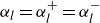 $\alpha _{l}=\alpha _{l}^+= \alpha _{l}^-$
. Therefore, we can have
$\alpha _{l}=\alpha _{l}^+= \alpha _{l}^-$
. Therefore, we can have
 \begin{equation} \boldsymbol{q}_{gg} = -\alpha _{g}^2\lambda _{g}\boldsymbol{\nabla }T_{g}. \end{equation}
Similarly, the contact area fraction between the internal plasma and the surrounding liquid can be expressed as $\alpha _{g}^+ \alpha _{l}^-$
. The interphase thermal conduction is expected to be determined by the two phases, thus we phenomenologically assign the effective interphase thermal conduction coefficient as
$\alpha _{g}^+ \alpha _{l}^-$
. The interphase thermal conduction is expected to be determined by the two phases, thus we phenomenologically assign the effective interphase thermal conduction coefficient as $\sqrt {\lambda _{g}\lambda _{l}}$
, a geometric average of
$\sqrt {\lambda _{g}\lambda _{l}}$
, a geometric average of $\lambda _{g}$
and
$\lambda _{g}$
and $\lambda _{l}$
. Assuming a local temperature difference
$\lambda _{l}$
. Assuming a local temperature difference $T_{g}^{+}-T_{l}^{-}$
over a small length scale
$T_{g}^{+}-T_{l}^{-}$
over a small length scale $\delta \boldsymbol{x}$
, the liquid-to-plasma flux
$\delta \boldsymbol{x}$
, the liquid-to-plasma flux $\boldsymbol{q}_{gl}$
can be estimated by
$\boldsymbol{q}_{gl}$
can be estimated by
 \begin{equation} \boldsymbol{q}_{gl} = -\alpha _{g}^+\alpha _{l}^-\sqrt {\lambda _{g}\lambda _{l}} \big ( T_{g}^{+}-T_{l}^{-} \big ) /\delta \boldsymbol{x}. \end{equation}
Equation (3.15) can be reformulated in two equivalent ways:
 \begin{align} \boldsymbol{q}_{gl} &= -\alpha _{g}^+\alpha _{l}^-\sqrt {\lambda _{g}\lambda _{l}} \big(\boldsymbol{\nabla }T_{g}+\big(T_{g}^{-}-T_{l}^{-}\big) /\delta \boldsymbol{x} \big), \qquad \text{or}\nonumber \\[3pt] &= -\alpha _{g}^+\alpha _{l}^-\sqrt {\lambda _{g}\lambda _{l}} \big( \boldsymbol{\nabla }T_{l}+\big(T_{g}^{+}-T_{l}^{+}\big) /\delta \boldsymbol{x} \big). \end{align}
In these forms, the local temperature difference between the plasma and liquid phases ( $T_{g}^{+}-T_{l}^{+}$
or
$T_{g}^{+}-T_{l}^{+}$
or $T_{g}^{-}-T_{l}^{-}$
) implies that
$T_{g}^{-}-T_{l}^{-}$
) implies that $\boldsymbol{q}_{gl}$
is also related to the exchange rate of internal energy from plasma to liquid,
$\boldsymbol{q}_{gl}$
is also related to the exchange rate of internal energy from plasma to liquid, $Q_{gl}$
, evaluated on the internal and external sides of the contact surface, respectively.
$Q_{gl}$
, evaluated on the internal and external sides of the contact surface, respectively.
To keep the notational symmetry, the liquid-to-liquid and plasma-to-liquid energy fluxes due to thermal conduction can be expressed as
 \begin{equation} \boldsymbol{q}_{ll} = -\alpha _{l}^{2}\lambda _{l}\boldsymbol{\nabla }T_{l}, \quad \boldsymbol{q}_{lg} = -\alpha _{l}^+\alpha _{g}^-\sqrt {\lambda _{g}\lambda _{l}}\big( T_{l}^{+}-T_{g}^{-} \big) /\delta \boldsymbol{x}. \end{equation}
The mixture thermal flux is then contributed by all of the fluxes within and between phases, i.e. $\boldsymbol{q}=\boldsymbol{q}_{gg}+\boldsymbol{q}_{gl}+\boldsymbol{q}_{lg}+\boldsymbol{q}_{ll}$
. It is worth noting that the temperature differences between the plasma and liquid phases in
$\boldsymbol{q}=\boldsymbol{q}_{gg}+\boldsymbol{q}_{gl}+\boldsymbol{q}_{lg}+\boldsymbol{q}_{ll}$
. It is worth noting that the temperature differences between the plasma and liquid phases in $\boldsymbol{q}_{lg}$
and
$\boldsymbol{q}_{lg}$
and $\boldsymbol{q}_{gl}$
cancel upon summation. Consequently, the final expression for
$\boldsymbol{q}_{gl}$
cancel upon summation. Consequently, the final expression for $\boldsymbol{q}$
can be simplified accordingly:
$\boldsymbol{q}$
can be simplified accordingly:
 \begin{equation} \boldsymbol{q} = -\alpha _{g}^{2}\lambda _{g}\boldsymbol{\nabla }T_{g}-\alpha _{g}\alpha _{l}\sqrt {\lambda _{g}\lambda _{l}}\,(\boldsymbol{\nabla }T_{g}+\boldsymbol{\nabla }T_{l})-\alpha _{l}^{2}\lambda _{l}\boldsymbol{\nabla }T_{l}. \end{equation}
This modelling approach has the desirable property that it reduces to Fick’s law $\boldsymbol{q}=- \lambda \boldsymbol{\nabla }T$
in the limit where the two phases are identical, thereby ensuring its consistency with the single-phase theory.
$\boldsymbol{q}=- \lambda \boldsymbol{\nabla }T$
in the limit where the two phases are identical, thereby ensuring its consistency with the single-phase theory.
The energy flux due to radiation diffusion is analogous to the conductive heat flux to some degree. In the optically thick limit, where the radiation can be described as a diffusion field, the radiation diffusion fluxes are proportional to the contact area between phases and the respective radiation diffusion coefficients ( $\chi _{r,g}, \chi _{r,l}$
). By direct analogy to the conductive heat flux form derived in (3.18), the radiation energy flux for the mixture can be written as
$\chi _{r,g}, \chi _{r,l}$
). By direct analogy to the conductive heat flux form derived in (3.18), the radiation energy flux for the mixture can be written as
 \begin{equation} \boldsymbol{F}_{\!r} = -(\alpha _{g}^{2}\chi _{r,g}+2\alpha _{g}\alpha _{l}\sqrt {\chi _{r,g}\chi _{r,l}}+\alpha _{l}^{2}\chi _{r,l})\,\boldsymbol{\nabla }T_{r}^{4}. \end{equation}
Because of the comparatively negligible thermal conduction coefficient and high opacity of the liquid, we set $\lambda _{l}\approx 0$
,
$\lambda _{l}\approx 0$
, $\omega _{r,l}\approx 0$
and
$\omega _{r,l}\approx 0$
and $\chi _{r,l}\approx 0$
in this paper. Accordingly, the radiative energy source, the conductive heat flux and the radiative diffusion flux yields a simplified model valid within the diffuse interface region:
$\chi _{r,l}\approx 0$
in this paper. Accordingly, the radiative energy source, the conductive heat flux and the radiative diffusion flux yields a simplified model valid within the diffuse interface region:
 \begin{equation} \begin{cases} \boldsymbol{q}=-\alpha _{g}^{2}\lambda _{g} \boldsymbol{\nabla }T_{g},\\[5pt] S_{r}=\alpha _{g}\omega _{r,g}\big( T_{r}^{4}-T_{g}^{4} \big), \\[5pt] \boldsymbol{F}_{\!r}=-\alpha _{g}^{2}\chi _{r,g} \boldsymbol{\nabla }T_{r}^{4}. \end{cases} \end{equation}
This simplified formulation preserves a continuous transition for the energy fluxes and sources from the plasma to the liquid, governed by the plasma volume fraction $\alpha _{g}$
. At the same time, it satisfies the required jump conditions at the interfaces.
$\alpha _{g}$
. At the same time, it satisfies the required jump conditions at the interfaces.
3.5. Summary of the model for plasma–liquid interactions
By applying the expressions of the energy fluxes and source in (3.20), we now rewrite the radiation two-phase flow model in (3.1) as
 \begin{equation} \begin{cases} \partial _{t} \alpha _{l}+\boldsymbol{u} \boldsymbol{\cdot }\boldsymbol{\nabla }\alpha _{l}= 0 , \\[5pt] \partial _{t} ( \rho _{l} \alpha _{l} ) +\boldsymbol{\nabla }\boldsymbol{\cdot }( \rho _{l} \alpha _{l}\boldsymbol{u}) =0 ,\\[5pt] \partial _{t} ( \rho _{g} \alpha _{g} ) +\boldsymbol{\nabla }\boldsymbol{\cdot }( \rho _{g} \alpha _{g}\boldsymbol{u}) =0 ,\\[5pt] \partial _{t} ( \rho \boldsymbol{u} ) +\boldsymbol{\nabla }\boldsymbol{\cdot }( \rho \boldsymbol{u}\boldsymbol{u} )+\boldsymbol{\nabla }\boldsymbol{\cdot }\left ((p+p_{r}) \boldsymbol {I}\right ) =\sigma \kappa\, \boldsymbol{\nabla }\phi , \\[5pt] \partial _{t} ( \rho e ) +\boldsymbol{\nabla }\boldsymbol{\cdot }( \rho e \boldsymbol{u} ) +p\,\boldsymbol{\nabla }\boldsymbol{\cdot }\boldsymbol{u}= \boldsymbol{\nabla }\boldsymbol{\cdot }\big(\alpha _{g}^{2}\lambda _{g} \boldsymbol{\nabla }T_{g}\big)+ \alpha _{g}\omega _{r,g}\big( T_{r}^{4}-T_{g}^{4} \big) , \\[5pt] \partial _{t} E_{r} +\boldsymbol{\nabla }\boldsymbol{\cdot }( E_{r} \boldsymbol{u} ) +p_{r}\boldsymbol{\nabla }\boldsymbol{\cdot }\boldsymbol{u}=\boldsymbol{\nabla }\boldsymbol{\cdot }\big(\alpha _{g}^{2}\chi _{r,g} \boldsymbol{\nabla }T_{r}^{4}\big) -\alpha _{g}\omega _{r,g}\big( T_{r}^{4}-T_{g}^{4} \big). \end{cases} \end{equation}
Although this model is derived for the mixture, it exhibits the correct asymptotic behaviour by reducing to standard single-phase models in the limit of $\alpha _{g}$
. It is straightforward that the system of equations in (3.21) converges to the Euler equation (2.3) for the pure liquid in the limit of vanishing plasma and radiation, while it recovers the RHD equations for a pure plasma (2.1) as
$\alpha _{g}$
. It is straightforward that the system of equations in (3.21) converges to the Euler equation (2.3) for the pure liquid in the limit of vanishing plasma and radiation, while it recovers the RHD equations for a pure plasma (2.1) as $\alpha _{g} \rightarrow 1$
.
$\alpha _{g} \rightarrow 1$
.
4. Numerical method
In order to numerically solve the radiation two-phase flow for plasma–liquid interactions described in (3.21), we employ an operator-splitting numerical algorithm (McLachlan & Quispel Reference McLachlan and Quispel2002). This approach is particularly effective for handling the multiphysics nature of the equations, where the characteristic time scales and numerical stiffnesses associated with convective transport differ significantly from those of diffusive processes. The method proceeds by separating the full system into two sequential sub-problems – a hyperbolic step and a parabolic step – and consequently allows us to use efficient numerical techniques to account for the distinct mathematical properties of each sub-problem.
In the hyperbolic step, we integrate the subsystem governing convection of the fluid and radiation. Note that the energy equations for fluid and radiation convection of (3.21) are not in the conservative form, primarily due to the pressure–work terms associated with fluid compressibility. In order to impose strict energy conservation, we instead consider the convection of the total energy density $\rho e_{t}$
, which is defined as
$\rho e_{t}$
, which is defined as $\rho e_{t}=\rho e+E_{r}+\rho \left |\boldsymbol{u} \right |^{2}/2$
. The governing equations for the hyperbolic system are
$\rho e_{t}=\rho e+E_{r}+\rho \left |\boldsymbol{u} \right |^{2}/2$
. The governing equations for the hyperbolic system are
 \begin{align} &\partial _{t} \alpha _{l}+\boldsymbol{\nabla }\boldsymbol{\cdot }\left ( \alpha _{l}\boldsymbol{u}\right )= \alpha _{l} \boldsymbol{\nabla }\boldsymbol{\cdot }\boldsymbol{u}, \\[-12pt]\nonumber \end{align}
 \begin{align} &\partial _{t} ( \rho _{l} \alpha _{l} ) +\boldsymbol{\nabla }\boldsymbol{\cdot }( \rho _{l} \alpha _{l}\boldsymbol{u}) =0 , \\[-12pt]\nonumber \end{align}
 \begin{align} &\partial _{t} ( \rho _{g} \alpha _{g} ) +\boldsymbol{\nabla }\boldsymbol{\cdot }( \rho _{g} \alpha _{g}\boldsymbol{u}) =0 , \\[-12pt]\nonumber \end{align}
 \begin{align} &\partial _{t} ( \rho \boldsymbol{u} ) +\boldsymbol{\nabla }\boldsymbol{\cdot }( \rho \boldsymbol{u}\boldsymbol{u} )+\boldsymbol{\nabla }\boldsymbol{\cdot }\left (p_{t} \boldsymbol{I}\right ) =\sigma \kappa\, \boldsymbol{\nabla }\phi, \\[-12pt]\nonumber \end{align}
 \begin{align} &\partial _{t} \left ( \rho e_{t}\right ) +\boldsymbol{\nabla }\boldsymbol{\cdot }\left ( \rho e_{t} \boldsymbol{u} \right ) + \boldsymbol{\nabla }\boldsymbol{\cdot }\left ( p_{t}\boldsymbol{u} \right ) = \sigma \kappa\, \boldsymbol{\nabla }\phi \boldsymbol{\cdot }\boldsymbol{u} , \end{align}
with the total pressure given by $p_{t}=p+p_{r}$
. Equation (4.1e
) is obtained by summing the energy equation of the fluid and radiation (3.21), and the dot product of (4.1d
) with the velocity vector; further details are provided in Appendix A.
$p_{t}=p+p_{r}$
. Equation (4.1e
) is obtained by summing the energy equation of the fluid and radiation (3.21), and the dot product of (4.1d
) with the velocity vector; further details are provided in Appendix A.
In the parabolic step, we integrate the subsystem governing thermal conduction and radiation diffusion:
 \begin{equation} \begin{cases} \partial _{t} ( \rho e ) = \boldsymbol{\nabla }\boldsymbol{\cdot }\big( \alpha _{g}^{2}\lambda _{g}\boldsymbol{\nabla }T_{g} \big)+\alpha _{g}\omega _{r,g}\big( T_{r}^{4}-T_{g}^{4} \big), \\[6pt] \partial _{t} E_{r} =\boldsymbol{\nabla }\boldsymbol{\cdot }\big( \alpha _{g}^{2}\chi _{r,g}\boldsymbol{\nabla }T_{r}^{4} \big) + \alpha _{g}\omega _{r,g}\big( T_{g}^{4}-T_{r}^{4} \big) . \end{cases} \end{equation}
In particular, an explicit scheme is implemented for the convection of fluid and radiation, with an implicit scheme for the thermal conduction and radiation diffusion; details are provided in the following subsections. Both the explicit scheme for (4.1) and the implicit scheme for (4.2) are embedded in a second-order Runge–Kutta scheme for time integration.
4.1. Hyperbolic step: convection of fluid and radiation
The convection equations (4.1) are discretised using a second-order finite-volume scheme with the numerical fluxes computed via the HLLC approximate Riemann solver (Toro Reference Toro2013). The characteristic wave speed $C_{\!s}$
is obtained from the eigenvalue of the hyperbolic system, computed from its Jacobian matrix; see Appendix B for details. The term for velocity divergence in the volume-fraction advection equation (4.1a
) is evaluated using the adapt-HLLC scheme (Johnsen & Colonius Reference Johnsen and Colonius2006). The surface tensions in (4.1d
) and (4.1e
) are treated as source terms and discretised by the central difference scheme. The time step
$C_{\!s}$
is obtained from the eigenvalue of the hyperbolic system, computed from its Jacobian matrix; see Appendix B for details. The term for velocity divergence in the volume-fraction advection equation (4.1a
) is evaluated using the adapt-HLLC scheme (Johnsen & Colonius Reference Johnsen and Colonius2006). The surface tensions in (4.1d
) and (4.1e
) are treated as source terms and discretised by the central difference scheme. The time step $\Delta t$
is chosen adaptively such that the Courant–Friedrichs–Lewy (CFL) condition is strictly satisfied:
$\Delta t$
is chosen adaptively such that the Courant–Friedrichs–Lewy (CFL) condition is strictly satisfied:
 \begin{equation} \Delta t=\mathrm{CFL}\times\min _{i\in D} \left \{ \frac {\sqrt [3]{V_{i}} }{\left | \boldsymbol{u}_{i} \right | +C_{s,i}} \right \} \!, \end{equation}
where the $\mathrm{CFL}$
number (
$\mathrm{CFL}$
number ( $=0.44$
) is a prescribed constant, the subscript
$=0.44$
) is a prescribed constant, the subscript $i$
denotes a Cartesian cell in the computational domain
$i$
denotes a Cartesian cell in the computational domain $D$
,
$D$
, $C_{\!s}=\sqrt {C^{2}+4p_{r}/(3\rho )}$
is the local wave speed, and
$C_{\!s}=\sqrt {C^{2}+4p_{r}/(3\rho )}$
is the local wave speed, and $V$
is the volume of the cell.
$V$
is the volume of the cell.
After solving the fluid and radiation convection explicitly, we update the conservative variables to an intermediate state, denoted by the superscript $*$
:
$*$
: $[\alpha_l^*, (\rho_l\alpha_l)^*, (\rho_g\alpha_g)^*, (\rho\boldsymbol{u})^*, (\rho e_{t})^*]^{\rm T}$
. The corresponding primitive variables at the intermediate state are also updated. From
$[\alpha_l^*, (\rho_l\alpha_l)^*, (\rho_g\alpha_g)^*, (\rho\boldsymbol{u})^*, (\rho e_{t})^*]^{\rm T}$
. The corresponding primitive variables at the intermediate state are also updated. From $(\rho e_{t})^*$
, the internal energy
$(\rho e_{t})^*$
, the internal energy $(\rho e)^*$
and radiation energy
$(\rho e)^*$
and radiation energy $(E_{r})^*$
of the mixture can then be calculated; see details in Appendix C.
$(E_{r})^*$
of the mixture can then be calculated; see details in Appendix C.
4.2. Parabolic step: thermal conduction and radiation diffusion
An implicit scheme is adopted for the time integration of the thermal conduction and radiation diffusion in (4.2). All the coefficients in the equations are linearised using the flow variables at the intermediate state:
 \begin{equation} \begin{cases} \displaystyle \frac {(\rho e)^{n+1}-(\rho e)^{*}}{\Delta t} = \boldsymbol{\nabla }\boldsymbol{\cdot }\big(\big(\alpha _{g}^{2}\lambda _{g}\big)^{*}\,\boldsymbol{\nabla }(T_{g})^{n+1}\big)+(\alpha _{g}\omega _{r,g})^{*} \,\big( T_{r}^{4}-T_{g}^{4} \big)^{n+1},\\[12pt] \displaystyle \frac { (E_{r} )^{n+1}- (E_{r} )^{*}}{\Delta t} =\boldsymbol{\nabla }\boldsymbol{\cdot }\big( \big(\alpha _{g}^{2}\chi _{r,g} \big)^{*}\,\boldsymbol{\nabla }\big(T_{r}^{4} \big)^{n+1}\big) + (\alpha _{g}\omega _{r,g})^{*}\, \big(T_{g}^{4}-T_{r}^{4}\big)^{n+1}. \end{cases} \end{equation}
The gradient and divergence terms are discretised using a central finite-difference scheme. By solving (4.4) iteratively, $\rho e$
and
$\rho e$
and $E_{r}$
are updated from the intermediate state to the
$E_{r}$
are updated from the intermediate state to the $n+1$
time step. Subsequently, by employing the EOS, all remaining conservative and primitive variables associated with energy, such as
$n+1$
time step. Subsequently, by employing the EOS, all remaining conservative and primitive variables associated with energy, such as $p$
,
$p$
, $p_{r}$
,
$p_{r}$
, $T_{g}$
and
$T_{g}$
and $T_{r}$
, are calculated for the
$T_{r}$
, are calculated for the $n+1$
time step, while those related to mass and momentum are retained from the intermediate state. This completes the numerical solution of the radiation two-phase flow system for plasma–liquid interactions.
$n+1$
time step, while those related to mass and momentum are retained from the intermediate state. This completes the numerical solution of the radiation two-phase flow system for plasma–liquid interactions.
5. Model validations
In this section, we validate the radiation two-phase flow model by simulating two types of flows: plasma single-phase flow and liquid–gas two-phase flow. The numerical results for each are compared against benchmark solutions from the literature.
5.1. Radiative shock tube
The profiles of a radiative shock problem at $0\ \mathrm{ns}$
(black solid lines and open squares) and
$0\ \mathrm{ns}$
(black solid lines and open squares) and $4.2\ \mathrm{ns}$
(red dashed lines and solid circles), in terms of (a) density, (b) plasma temperature, and (c) radiation temperature. The symbols and lines denote numerical and semi-analytical solutions, respectively. Note that the symbols are sampled at every
$4.2\ \mathrm{ns}$
(red dashed lines and solid circles), in terms of (a) density, (b) plasma temperature, and (c) radiation temperature. The symbols and lines denote numerical and semi-analytical solutions, respectively. Note that the symbols are sampled at every $8$
th grid point for visual clarity.
$8$
th grid point for visual clarity.

To validate the radiation transport in our model, we consider a one-dimensional radiative shock tube problem, where the radiation energy fluxes and radiation pressure significantly affect the hydrodynamics. As illustrated in figure 2, a low-temperature low-density plasma (with density $\rho ^{L}$
, temperature
$\rho ^{L}$
, temperature $T^{L}$
and velocity
$T^{L}$
and velocity $u^{L}$
) is initially impacting a high-temperature high-density plasma (with density
$u^{L}$
) is initially impacting a high-temperature high-density plasma (with density $\rho ^{R}$
, temperature
$\rho ^{R}$
, temperature $T^{R}$
and velocity
$T^{R}$
and velocity $u^{R}$
). This configuration is designed to produce a stationary radiative shock at
$u^{R}$
). This configuration is designed to produce a stationary radiative shock at $x=0 \,\unicode{x03BC} \mathrm{m}$
, the solution of which can be compared with the semi-analytical result from Lowrie & Edwards (Reference Lowrie and Edwards2008).
$x=0 \,\unicode{x03BC} \mathrm{m}$
, the solution of which can be compared with the semi-analytical result from Lowrie & Edwards (Reference Lowrie and Edwards2008).
Because the fluid system only has one phase, i.e. plasma, we set $\alpha _{g}=1$
everywhere in the domain. The properties of the plasma are an adiabatic index
$\alpha _{g}=1$
everywhere in the domain. The properties of the plasma are an adiabatic index $\gamma _{g} = 5/3$
, a molar mass
$\gamma _{g} = 5/3$
, a molar mass $M_{g} = 2\ \mathrm{g\,mol}^{-1}$
, and a constant ionisation degree
$M_{g} = 2\ \mathrm{g\,mol}^{-1}$
, and a constant ionisation degree $Z_{g} = 1$
, which determine
$Z_{g} = 1$
, which determine $c_{v,g} = 1.247\times 10^8\ \mathrm{cm}^{2}\ \mathrm{s}^{-2}\ \mathrm{K}^{-1}$
. Thermal conduction is neglected (i.e.
$c_{v,g} = 1.247\times 10^8\ \mathrm{cm}^{2}\ \mathrm{s}^{-2}\ \mathrm{K}^{-1}$
. Thermal conduction is neglected (i.e. $\lambda _{g}=0$
). The diffusion coefficient and the exchange rate of the radiative energy are
$\lambda _{g}=0$
). The diffusion coefficient and the exchange rate of the radiative energy are $\chi _{r,g} = 1.268\times 10^{7}\ \mathrm{cm}^{2}\,\mathrm{s}^{-1}$
and
$\chi _{r,g} = 1.268\times 10^{7}\ \mathrm{cm}^{2}\,\mathrm{s}^{-1}$
and $\omega _{r,g} = 1.268\times 10^{13}\ \mathrm{s}^{-1}$
, respectively. The initial conditions are defined by a step function at
$\omega _{r,g} = 1.268\times 10^{13}\ \mathrm{s}^{-1}$
, respectively. The initial conditions are defined by a step function at $x=0\, \unicode{x03BC} \mathrm{m}$
, as illustrated in figure 2. The radiation is initially set in thermal equilibrium with the plasma (i.e.
$x=0\, \unicode{x03BC} \mathrm{m}$
, as illustrated in figure 2. The radiation is initially set in thermal equilibrium with the plasma (i.e. $T_{r}=T$
). The initial flow parameters of the plasma are
$T_{r}=T$
). The initial flow parameters of the plasma are
 \begin{equation} \begin{cases} \rho ^{R} = 2.286\ \mathrm{g}\,\mathrm{cm}^{-3},\quad T^{R} = 2.411\times 10^6\ \mathrm{K},\quad u^{R} = 1.11\times 10^7\ \mathrm{cm}\,\mathrm{s}^{-1}, \\[3pt] \rho ^{L} = 1\ \mathrm{g}\,\mathrm{cm}^{-3},\quad T^{L} = 1.16\times 10^6\ \mathrm{K},\quad u^{L} = 2.536\times 10^7\ \mathrm{cm}\,\mathrm{s}^{-1}. \end{cases} \end{equation}
The computation is performed in a domain $ [-300,\ 300 ]\,\unicode{x03BC} \mathrm{m}$
, discretised by a uniform grid of
$ [-300,\ 300 ]\,\unicode{x03BC} \mathrm{m}$
, discretised by a uniform grid of $2000$
points.
$2000$
points.
Figure 2 presents numerical results at $t = 4.2\ \mathrm{ns}$
in terms of density, plasma temperature and radiation temperature. These results are superimposed with the semi-analytical solution by Lowrie & Edwards (Reference Lowrie and Edwards2008). Obviously, the numerical results are in excellent agreement with the theoretical prediction, with respect to the position of the stationary shock and the diffusion profiles on either side of the discontinuity. The comparison demonstrates that the proposed model can be reduced to an RHD model for single phase, and successfully captures complex plasma flow structures, including radiative shocks.
$t = 4.2\ \mathrm{ns}$
in terms of density, plasma temperature and radiation temperature. These results are superimposed with the semi-analytical solution by Lowrie & Edwards (Reference Lowrie and Edwards2008). Obviously, the numerical results are in excellent agreement with the theoretical prediction, with respect to the position of the stationary shock and the diffusion profiles on either side of the discontinuity. The comparison demonstrates that the proposed model can be reduced to an RHD model for single phase, and successfully captures complex plasma flow structures, including radiative shocks.
5.2. Blast wave with thermal conduction
(a) Density, (b) relative density error $|\rho ^{N}-\rho ^{A}|/\rho ^{A}$
, (c) temperature, and (d) relative temperature error
$|\rho ^{N}-\rho ^{A}|/\rho ^{A}$
, (c) temperature, and (d) relative temperature error $|T^{N}-T^{A}|/T^{A}$
for the Reinicke–Meyer-ter-Vehn blast wave problem at
$|T^{N}-T^{A}|/T^{A}$
for the Reinicke–Meyer-ter-Vehn blast wave problem at $0.52\ \mathrm{ns}$
, where superscripts
$0.52\ \mathrm{ns}$
, where superscripts $N$
and
$N$
and $A$
represent numerical and semi-analytical results, respectively.
$A$
represent numerical and semi-analytical results, respectively.

To validate the thermal conduction in our model, we consider the Sedov–Taylor point explosion with nonlinear thermal conduction, also referred to as the Reinicke–Meyer-ter-Vehn problem, which only involves the plasma phase and has the semi-analytical solution for the blast wave (Reinicke & Meyer-ter-Vehn Reference Reinicke and Meyer-ter-Vehn1991). To avoid the singularity of a point explosion, the initial condition for the simulation is taken from the semi-analytical solution right after the bang time. At this moment, the stationary and uniform ambient plasma is about to be swept through by a tiny and rapidly expanding spherical blast wave.
The plasma is modelled as an ideal gas with adiabatic index $\gamma _{g} = 1.25$
, molar mass
$\gamma _{g} = 1.25$
, molar mass $M_{g} = 1\ \mathrm{g\,mol}^{-1}$
and ionisation degree zero, giving a specific heat capacity at constant volume
$M_{g} = 1\ \mathrm{g\,mol}^{-1}$
and ionisation degree zero, giving a specific heat capacity at constant volume $c_{v,g} = 3.326\times 10^8\ \mathrm{cm}^{2}\ \mathrm{s}^{-2}\ \mathrm{K}^{-1}$
. The radiation transport is not excluded from this problem; accordingly, the radiation energy
$c_{v,g} = 3.326\times 10^8\ \mathrm{cm}^{2}\ \mathrm{s}^{-2}\ \mathrm{K}^{-1}$
. The radiation transport is not excluded from this problem; accordingly, the radiation energy $E_{r}$
, the radiation pressure
$E_{r}$
, the radiation pressure $p_{r}$
, the radiative energy exchange rate
$p_{r}$
, the radiative energy exchange rate $\omega _{r,g}$
, and the radiative energy diffusion coefficient
$\omega _{r,g}$
, and the radiative energy diffusion coefficient $\chi _{r,g}$
for the plasma are all set to zero. The thermal conduction coefficient follows a nonlinear power-law function of density and temperature as recommended by Reinicke & Meyer-ter-Vehn (Reference Reinicke and Meyer-ter-Vehn1991), i.e.
$\chi _{r,g}$
for the plasma are all set to zero. The thermal conduction coefficient follows a nonlinear power-law function of density and temperature as recommended by Reinicke & Meyer-ter-Vehn (Reference Reinicke and Meyer-ter-Vehn1991), i.e. $\lambda _{g} = \rho _g^{-2}T_g^{6.5}\ (\text{in }\mathrm{g}\boldsymbol{\, }\mathrm{cm}\boldsymbol{\, }\mathrm{s}^{-3}\rm\, K^{-1})$
, where
$\lambda _{g} = \rho _g^{-2}T_g^{6.5}\ (\text{in }\mathrm{g}\boldsymbol{\, }\mathrm{cm}\boldsymbol{\, }\mathrm{s}^{-3}\rm\, K^{-1})$
, where $\rho _{g}$
is in
$\rho _{g}$
is in $\mathrm{g}\,\mathrm{cm}^{-3}$
, and
$\mathrm{g}\,\mathrm{cm}^{-3}$
, and $T_{g}$
is in
$T_{g}$
is in $\mathrm{K}$
. Axisymmetric simulations are performed in 2-D cylindrical coordinates (
$\mathrm{K}$
. Axisymmetric simulations are performed in 2-D cylindrical coordinates ( $(r,z)$
plane). The initial condition corresponds to the semi-analytical solution at
$(r,z)$
plane). The initial condition corresponds to the semi-analytical solution at $t = 0.2\ \mathrm{ns}$
, when the shock front has radius
$t = 0.2\ \mathrm{ns}$
, when the shock front has radius $0.225\ \mathrm{cm}$
, and the heat front has radius
$0.225\ \mathrm{cm}$
, and the heat front has radius $0.45\ \mathrm{cm}$
. The computational domain is
$0.45\ \mathrm{cm}$
. The computational domain is $ [ 0, 1 ] \times [ 0, 1 ]\ \mathrm{cm}^2$
, and is discretised by
$ [ 0, 1 ] \times [ 0, 1 ]\ \mathrm{cm}^2$
, and is discretised by $2048\times 2048$
grid points.
$2048\times 2048$
grid points.
Figures 3( $a$
) and 3(
$a$
) and 3( $c$
) illustrate the distributions of density and temperature at
$c$
) illustrate the distributions of density and temperature at $t = 0.52\ \mathrm{ns}$
. As predicted by Reinicke & Meyer-ter-Vehn (Reference Reinicke and Meyer-ter-Vehn1991), the shock front reached radius
$t = 0.52\ \mathrm{ns}$
. As predicted by Reinicke & Meyer-ter-Vehn (Reference Reinicke and Meyer-ter-Vehn1991), the shock front reached radius $0.45\ \mathrm{cm}$
and the heat front
$0.45\ \mathrm{cm}$
and the heat front $0.9\ \mathrm{cm}$
. The corresponding relative errors in density and temperature are shown in figures 3(
$0.9\ \mathrm{cm}$
. The corresponding relative errors in density and temperature are shown in figures 3( $b$
) and 3(
$b$
) and 3( $d$
), respectively. The maximum errors, which do not exceed
$d$
), respectively. The maximum errors, which do not exceed $5\,\%$
, are localised at the discontinuities of the shock and heat front, and are attributed to finite grid resolution. The good agreement with the semi-analytical solution demonstrates the capability of the proposed model to accurately deal with nonlinear thermal conduction.
$5\,\%$
, are localised at the discontinuities of the shock and heat front, and are attributed to finite grid resolution. The good agreement with the semi-analytical solution demonstrates the capability of the proposed model to accurately deal with nonlinear thermal conduction.
5.3. Bubble collapse induced by shock wave
The shock-induced collapse of a gas bubble in water, where a planar shock wave propagating through the water interacts with an underwater gas bubble, has been extensively studied by simulations (Nourgaliev, Dinh & Theofanous Reference Nourgaliev, Dinh and Theofanous2006; Hawker & Ventikos Reference Hawker and Ventikos2012; Bo & Grove Reference Bo and Grove2014). This classic problem is used here to verify that the governing equations of the proposed model correctly reduce to those for compressible two-phase flows. In this case, thermal conduction, radiation transport and surface tension are neglected. Consequently, all associated variables and coefficients – including radiation energy $E_{r}$
, radiation pressure
$E_{r}$
, radiation pressure $p_{r}$
, thermal conduction coefficient
$p_{r}$
, thermal conduction coefficient $\lambda _{g}$
, radiative energy diffusion coefficient
$\lambda _{g}$
, radiative energy diffusion coefficient $\chi _{r,g}$
, radiative energy exchange rate
$\chi _{r,g}$
, radiative energy exchange rate $\omega _{r,g}$
, and surface tension coefficient
$\omega _{r,g}$
, and surface tension coefficient $\sigma$
– are set to zero. Regarding the EOS, the water is described by the SG model (parameters are listed in table 1), while the gas phase is treated as an ideal gas with
$\sigma$
– are set to zero. Regarding the EOS, the water is described by the SG model (parameters are listed in table 1), while the gas phase is treated as an ideal gas with $\gamma _{g}=1.4$
.
$\gamma _{g}=1.4$
.
The simulation is performed in 2-D Cartesian coordinates. Initially, a circular bubble is centred at $ ( 0, 0 )\ \mathrm{mm}$
with radius
$ ( 0, 0 )\ \mathrm{mm}$
with radius $3\ \mathrm{mm}$
. The density and pressure inside the bubble are
$3\ \mathrm{mm}$
. The density and pressure inside the bubble are $1\ \mathrm{kg}\,\mathrm{m}^{-3}$
and
$1\ \mathrm{kg}\,\mathrm{m}^{-3}$
and $10^{5}\ \mathrm{Pa}$
, respectively. An incident shock wave is positioned at
$10^{5}\ \mathrm{Pa}$
, respectively. An incident shock wave is positioned at $5.4\ \mathrm{mm}$
to the left of the bubble centre initially, and propagates to the
$5.4\ \mathrm{mm}$
to the left of the bubble centre initially, and propagates to the $x+$
direction. The right-hand (with the superscript
$x+$
direction. The right-hand (with the superscript $R$
) and left-hand (with the superscript
$R$
) and left-hand (with the superscript $L$
) sides of the shock are initialised as follows:
$L$
) sides of the shock are initialised as follows:
 \begin{equation} \begin{cases} \rho ^{R} = 1000\ \mathrm{kg}\,\mathrm{m}^{-3},\quad p^{R} = 10^{5}\ \mathrm{Pa},\quad u^{R} = 0, \\[3pt] \rho ^{L} = 1323.65\ \mathrm{kg}\,\mathrm{m}^{-3},\quad p^{L} = 1.9\times 10^{9}\ \mathrm{Pa},\quad u^{L} = 681.58\ \mathrm{m}\,\mathrm{s}^{-1}. \end{cases} \end{equation}
The computational domain spans $ [ -15, 15 ]\times [ -15, 15 ]\ \mathrm{mm}^2$
, and the bubble radius (
$ [ -15, 15 ]\times [ -15, 15 ]\ \mathrm{mm}^2$
, and the bubble radius ( $3\ \mathrm{mm}$
) is initially discretised by
$3\ \mathrm{mm}$
) is initially discretised by $800$
grid points.
$800$
grid points.
Figure 4 demonstrates different stages of the shock-induced bubble collapse in the simulation, visualised by pressure contours and numerical schlieren. Upon shock impact, a reflected rarefaction wave forms in the liquid, and a transmitted shock develops inside the bubble, as shown in figure 4( $a$
). At the same time, a re-entrant liquid jet forms at the left-hand side of the bubble, and propagates in the same direction as the incident shock, as shown in figure 4(
$a$
). At the same time, a re-entrant liquid jet forms at the left-hand side of the bubble, and propagates in the same direction as the incident shock, as shown in figure 4( $b$
). Upon impact of the jet with the rear interface of the bubble, a water-hammer shock is generated (see e.g.
$b$
). Upon impact of the jet with the rear interface of the bubble, a water-hammer shock is generated (see e.g. $t=3.9 \,\unicode{x03BC} \mathrm{s}$
in figure 4
$t=3.9 \,\unicode{x03BC} \mathrm{s}$
in figure 4 $c$
). The characteristic parameters of this event include the collision time
$c$
). The characteristic parameters of this event include the collision time $t_c$
, the water-hammer shock pressure
$t_c$
, the water-hammer shock pressure $p_w$
, and the jet speed
$p_w$
, and the jet speed $v_{\!j}$
at the instant of impact. Subsequently, the jet penetrates the bubble and merges with the surrounding liquid, while secondary jets gradually develop (see figure 4
$v_{\!j}$
at the instant of impact. Subsequently, the jet penetrates the bubble and merges with the surrounding liquid, while secondary jets gradually develop (see figure 4 $d$
). These flow features closely resemble the numerical results reported in Hawker & Ventikos (Reference Hawker and Ventikos2012). A quantitative comparison on
$d$
). These flow features closely resemble the numerical results reported in Hawker & Ventikos (Reference Hawker and Ventikos2012). A quantitative comparison on $t_c$
,
$t_c$
, $v_{\!j}$
and
$v_{\!j}$
and $p_w$
with the literature is provided in table 2. Good agreement is achieved for
$p_w$
with the literature is provided in table 2. Good agreement is achieved for $t_c$
and
$t_c$
and $v_{\!j}$
, while
$v_{\!j}$
, while $p_w$
is relatively lower in the present simulation, primarily due to coarser spatial resolution. The results confirm that the proposed radiation two-phase flow model correctly reduces to a standard compressible two-phase flow formulation when the radiation-specific terms are disabled. Furthermore, the good agreement with expected flow dynamics validates the core flow solver and the implementation of the EOS before the coupling with radiation transport and thermal conduction is introduced.
$p_w$
is relatively lower in the present simulation, primarily due to coarser spatial resolution. The results confirm that the proposed radiation two-phase flow model correctly reduces to a standard compressible two-phase flow formulation when the radiation-specific terms are disabled. Furthermore, the good agreement with expected flow dynamics validates the core flow solver and the implementation of the EOS before the coupling with radiation transport and thermal conduction is introduced.
Shock-induced bubble collapse compared to prior simulations: collision time ( $t_{c}$
), jet speed at collision (
$t_{c}$
), jet speed at collision ( $v_{\!j}$
), and water-hammer shock pressure (
$v_{\!j}$
), and water-hammer shock pressure ( $p_{w}$
).
$p_{w}$
).

Table 2. Long description
A table comparing shock-induced bubble collapse parameters across different studies. The table has five rows and three columns. The columns are labeled t subscript c (microseconds), v subscript j (meters per second), and p subscript wh (gigapascals). The rows are labeled Present, Lin et al. (2017), Hawker & Ventikos (2012), Bo & Grove (2014), and Nourgaliev et al. (2006). Row 1: Present, t subscript c 3.70, v subscript j 2837, p subscript wh 5.03. Row 2: Lin et al. (2017), t subscript c 3.70, v subscript j 2832, p subscript wh 5.90. Row 3: Hawker & Ventikos (2012), t subscript c 3.66, v subscript j 2810, p subscript wh 5.89. Row 4: Bo & Grove (2014), t subscript c 3.70, v subscript j 2830, p subscript wh not provided. Row 5: Nourgaliev et al. (2006), t subscript c 3.69, v subscript j 2850, p subscript wh 10.1.
Numerical results of bubble collapse induced by a planar shock with respect to pressure (upper half) and numerical schlieren (lower half) at (a) $2.2\,\unicode{x03BC} \mathrm{s}$
, (b)
$2.2\,\unicode{x03BC} \mathrm{s}$
, (b) $3.7\,\unicode{x03BC} \mathrm{s}$
, (c)
$3.7\,\unicode{x03BC} \mathrm{s}$
, (c) $3.9\,\unicode{x03BC} \mathrm{s}$
, (d)
$3.9\,\unicode{x03BC} \mathrm{s}$
, (d) $4.1 \,\unicode{x03BC} \mathrm{s}$
. The red lines represent the bubble interfaces (by
$4.1 \,\unicode{x03BC} \mathrm{s}$
. The red lines represent the bubble interfaces (by $\alpha _{g} = 0.5$
).
$\alpha _{g} = 0.5$
).

5.4. Droplet oscillation driven by surface tension
Due to the imbalance in surface tension, an initially elliptical droplet oscillates periodically, converting between potential and kinetic energy (Garrick et al. Reference Garrick, Owkes and Regele2017). The oscillation period can be analytically obtained (Fyfe, Oran & Fritts Reference Fyfe, Oran and Fritts1988):
 \begin{equation} t_{os}=2\pi \sqrt {\frac {(\rho _{l}+\rho _{g})R^{3}}{\big( o^{3}-o \big)\sigma }}, \end{equation}
where $o$
is the oscillation mode, and
$o$
is the oscillation mode, and $R$
is the radius of the droplet at equilibrium. We employ this case to validate the surface tension model.
$R$
is the radius of the droplet at equilibrium. We employ this case to validate the surface tension model.
Droplet oscillation: ( $a$
) evolution of the droplet over an oscillation period, where
$a$
) evolution of the droplet over an oscillation period, where $A$
and
$A$
and $B$
denote the initial semi-axes; (
$B$
denote the initial semi-axes; ( $b$
) kinetic energy of the droplet.
$b$
) kinetic energy of the droplet.

In the droplet oscillation, thermal conduction and radiation transport are absent; therefore, all corresponding variables and coefficients ( $E_{r}, p_{r}, \lambda _{g}, \chi _{r,g}, \omega _{r,g}$
) are set to zero in the simulation. For the EOS, the droplet is modelled as water by the SG model (see table 1), while the gas phase is treated as an ideal gas with
$E_{r}, p_{r}, \lambda _{g}, \chi _{r,g}, \omega _{r,g}$
) are set to zero in the simulation. For the EOS, the droplet is modelled as water by the SG model (see table 1), while the gas phase is treated as an ideal gas with $\gamma _{g}=1.33$
. The surface tension coefficient of the droplet is fixed at
$\gamma _{g}=1.33$
. The surface tension coefficient of the droplet is fixed at $\sigma = 500\ \mathrm{mN\,m}^{-1}$
. The simulation is performed in 2-D Cartesian coordinates. Initially, the elliptical droplet is centred at
$\sigma = 500\ \mathrm{mN\,m}^{-1}$
. The simulation is performed in 2-D Cartesian coordinates. Initially, the elliptical droplet is centred at $ ( 0, 0 )\ \unicode{x03BC} \mathrm{m}$
with the semi-axes
$ ( 0, 0 )\ \unicode{x03BC} \mathrm{m}$
with the semi-axes $A = 1.2\,\unicode{x03BC} \mathrm{m}$
and
$A = 1.2\,\unicode{x03BC} \mathrm{m}$
and $B = 0.8\,\unicode{x03BC} \mathrm{m}$
, resulting in droplet radius
$B = 0.8\,\unicode{x03BC} \mathrm{m}$
, resulting in droplet radius $R = 0.9798\,\unicode{x03BC} \mathrm{m}$
at equilibrium. The initial pressure of both the droplet and the ambient gas is set at
$R = 0.9798\,\unicode{x03BC} \mathrm{m}$
at equilibrium. The initial pressure of both the droplet and the ambient gas is set at $1.3\times 10^{5}\ \mathrm{Pa}$
, while the densities of the two phases are
$1.3\times 10^{5}\ \mathrm{Pa}$
, while the densities of the two phases are $1073.55\ \mathrm{kg}\,\mathrm{m}^{-3}$
and
$1073.55\ \mathrm{kg}\,\mathrm{m}^{-3}$
and $0.74\ \mathrm{kg}\,\mathrm{m}^{-3}$
, respectively. To exploit symmetry of the oscillation, only a quarter of the physical domain (
$0.74\ \mathrm{kg}\,\mathrm{m}^{-3}$
, respectively. To exploit symmetry of the oscillation, only a quarter of the physical domain ( $ [ 0, 5 ]\times [ 0, 5 ]\,\unicode{x03BC} \mathrm{m}^2$
) is simulated, with uniform mesh resolution
$ [ 0, 5 ]\times [ 0, 5 ]\,\unicode{x03BC} \mathrm{m}^2$
) is simulated, with uniform mesh resolution $2\ \text{nm}$
.
$2\ \text{nm}$
.
Figure 5( $a$
) shows snapshots of the droplet shapes at different times over one oscillation period, corresponding to the phase values
$a$
) shows snapshots of the droplet shapes at different times over one oscillation period, corresponding to the phase values $0$
,
$0$
, $\pi /2$
,
$\pi /2$
, $\pi$
,
$\pi$
, $3\pi /2$
and
$3\pi /2$
and $2\pi$
respectively. An oscillation mode
$2\pi$
respectively. An oscillation mode $o=2$
is observed. The periodicity of the droplet oscillation is quantitatively illustrated in figure 5(
$o=2$
is observed. The periodicity of the droplet oscillation is quantitatively illustrated in figure 5( $b$
), in terms of the kinetic energy (
$b$
), in terms of the kinetic energy ( $\int (\rho _{l}\alpha _{l}\left | \boldsymbol{u} \right | ^{2}/2)\,\mathrm{d}x\,\mathrm{d}y$
) versus time. A gradual decay of the oscillation amplitude is observed due to numerical dissipation, consistent with the findings in other studies (Garrick et al. Reference Garrick, Owkes and Regele2017; Long, Cai & Pan Reference Long, Cai and Pan2023). The oscillation period in simulation is
$\int (\rho _{l}\alpha _{l}\left | \boldsymbol{u} \right | ^{2}/2)\,\mathrm{d}x\,\mathrm{d}y$
) versus time. A gradual decay of the oscillation amplitude is observed due to numerical dissipation, consistent with the findings in other studies (Garrick et al. Reference Garrick, Owkes and Regele2017; Long, Cai & Pan Reference Long, Cai and Pan2023). The oscillation period in simulation is $118.4\ \mathrm{ns}$
, with relative error
$118.4\ \mathrm{ns}$
, with relative error $2.7\,\%$
compared to the theoretical prediction
$2.7\,\%$
compared to the theoretical prediction $115.3\ \mathrm{ns}$
. This demonstrates that the continuous surface tension incorporated in the present model accurately captures capillary effects.
$115.3\ \mathrm{ns}$
. This demonstrates that the continuous surface tension incorporated in the present model accurately captures capillary effects.
6. Nanosecond laser pulse irradiates tin droplet
( $a$
) Schematic of axisymmetric simulations of laser–droplet interactions. Cross-sectional shadowgraphs of the droplet at times ranging from
$a$
) Schematic of axisymmetric simulations of laser–droplet interactions. Cross-sectional shadowgraphs of the droplet at times ranging from $t=0.1\ \unicode{x03BC} \mathrm{s}$
to
$t=0.1\ \unicode{x03BC} \mathrm{s}$
to $t=1.6\ \unicode{x03BC} \mathrm{s}$
: (
$t=1.6\ \unicode{x03BC} \mathrm{s}$
: ( $b$
–
$b$
– $g$
) with surface tension, and (
$g$
) with surface tension, and ( $h$
–
$h$
– $m$
) without surface tension. All images have the same spatial scale, as shown in (
$m$
) without surface tension. All images have the same spatial scale, as shown in ( $a$
).
$a$
).

We use the proposed model to simulate an experimentally relevant pre-pulse scenario in LPP-EUV lithography, in which a tin droplet is irradiated by a nanosecond laser pulse and deforms into a thin sheet. The simulation is configured as an axisymmetric case with parameters matched to the systematic experimental work of Kurilovich et al. (Reference Kurilovich, Klein, Torretti, Lassise, Hoekstra, Ubachs, Gelderblom and Versolato2016). The initial configuration is sketched in figure 6( $a$
). Specifically, a
$a$
). Specifically, a $7\ \mathrm{mJ}$
Nd:YAG laser pulse with wavelength
$7\ \mathrm{mJ}$
Nd:YAG laser pulse with wavelength $1064\ \mathrm{nm}$
is employed, with duration
$1064\ \mathrm{nm}$
is employed, with duration $10\ \mathrm{ns}$
full width at half maximum (FWHM), and focal spot size
$10\ \mathrm{ns}$
full width at half maximum (FWHM), and focal spot size $115\,\unicode{x03BC} \mathrm{m}$
FWHM on the target, i.e. a tin (
$115\,\unicode{x03BC} \mathrm{m}$
FWHM on the target, i.e. a tin ( $\rho _l = 6.92\ \mathrm{g\,cm}^{-3}$
) droplet with diameter
$\rho _l = 6.92\ \mathrm{g\,cm}^{-3}$
) droplet with diameter $D = 50\,\unicode{x03BC} \mathrm{m}$
. The laser is modelled by using a ray-tracing approach, in which the beam is represented by over 20 000 individual rays that propagate geometrically through the plasma, each carrying a fraction of the total pulse energy. For this purpose, we adopt the ray-tracing methodology detailed in our earlier work (Tao et al. Reference Tao2025). Energy deposition in the plasma occurs primarily through inverse bremsstrahlung absorption. This process depends on the local plasma temperature and electron number density, and is incorporated into the model as a space- and time-dependent source term on the right-hand side of the mixture energy equation in (3.21).
$D = 50\,\unicode{x03BC} \mathrm{m}$
. The laser is modelled by using a ray-tracing approach, in which the beam is represented by over 20 000 individual rays that propagate geometrically through the plasma, each carrying a fraction of the total pulse energy. For this purpose, we adopt the ray-tracing methodology detailed in our earlier work (Tao et al. Reference Tao2025). Energy deposition in the plasma occurs primarily through inverse bremsstrahlung absorption. This process depends on the local plasma temperature and electron number density, and is incorporated into the model as a space- and time-dependent source term on the right-hand side of the mixture energy equation in (3.21).
Numerical results of laser-droplet interaction at ( $a$
)
$a$
) $2\ \mathrm{ns}$
and (
$2\ \mathrm{ns}$
and ( $b$
)
$b$
) $10\ \mathrm{ns}$
, in terms of density (upper half) and temperature (lower half). The arrows denote velocity vectors, and the black lines represent the droplet shape (by
$10\ \mathrm{ns}$
, in terms of density (upper half) and temperature (lower half). The arrows denote velocity vectors, and the black lines represent the droplet shape (by $\alpha _{l}=0.5$
).
$\alpha _{l}=0.5$
).

When the laser irradiates the tin droplet, plasma is generated via vaporisation and ionisation – processes not yet self-consistently included in the current model. A plasma layer is rapidly established surrounding the droplet, and blocks the laser from directly shining on the droplet surface, since a laser is unable to propagate beyond its critical density in a plasma (Kruer Reference Kruer1988). As a result, the laser energy is then deposited in the plasma only. To mimic the effects of phase change and plasma formation, we initialise a thin, high-density layer of ionised tin on the laser-irradiated (left-hand) surface of the droplet. The layer of high-density tin plasma is $1\,\unicode{x03BC} \mathrm{m}$
thick, with density
$1\,\unicode{x03BC} \mathrm{m}$
thick, with density $1\ \mathrm{g}\,\mathrm{cm}^{-3}$
on average, providing a simplified but typical representation of the initial plasma that absorbs incident laser energy. It is noteworthy that the mass of this layer that we initialise is consistent with experimental observations, i.e. less than 1 % of the droplet mass is ablated during the pre-pulse stage (Kurilovich et al. Reference Kurilovich, Klein, Torretti, Lassise, Hoekstra, Ubachs, Gelderblom and Versolato2016).
$1\ \mathrm{g}\,\mathrm{cm}^{-3}$
on average, providing a simplified but typical representation of the initial plasma that absorbs incident laser energy. It is noteworthy that the mass of this layer that we initialise is consistent with experimental observations, i.e. less than 1 % of the droplet mass is ablated during the pre-pulse stage (Kurilovich et al. Reference Kurilovich, Klein, Torretti, Lassise, Hoekstra, Ubachs, Gelderblom and Versolato2016).
The tin droplet is modelled as an SG with the parameters listed in table 1 and the surface tension coefficient $\sigma =538\ \mathrm{mN\,m}^{-1}$
, while the tin plasma is treated as an ideal gas with
$\sigma =538\ \mathrm{mN\,m}^{-1}$
, while the tin plasma is treated as an ideal gas with $\gamma _{g}=5/3$
and
$\gamma _{g}=5/3$
and $M_{g} = 118.71\ \mathrm{g\,mol}^{-1}$
. The ionisation degree (
$M_{g} = 118.71\ \mathrm{g\,mol}^{-1}$
. The ionisation degree ( $Z_{g}$
) is determined using the Thomas–Fermi model (More Reference More1985), the thermal conduction coefficient (
$Z_{g}$
) is determined using the Thomas–Fermi model (More Reference More1985), the thermal conduction coefficient ( $\lambda _{g}$
) follows the Spitzer–Härm theory (Spitzer & Härm Reference Spitzer and Härm1953), and the radiative transport coefficients (
$\lambda _{g}$
) follows the Spitzer–Härm theory (Spitzer & Härm Reference Spitzer and Härm1953), and the radiative transport coefficients ( $\chi _{r,g}$
,
$\chi _{r,g}$
, $\omega _{r,g}$
) are evaluated using the empirical formulae from Tsakiris & Eidmann (Reference Tsakiris and Eidmann1987); see details in Appendix D. Radiation is initially set to be in thermal equilibrium with the materials. The computational domain spans
$\omega _{r,g}$
) are evaluated using the empirical formulae from Tsakiris & Eidmann (Reference Tsakiris and Eidmann1987); see details in Appendix D. Radiation is initially set to be in thermal equilibrium with the materials. The computational domain spans $ [0, 300 ]\ \unicode{x03BC} \mathrm{m}$
in the radial direction (
$ [0, 300 ]\ \unicode{x03BC} \mathrm{m}$
in the radial direction ( $r$
), and
$r$
), and $ [-300, 300 ] \,\unicode{x03BC} \mathrm{m}$
in the axial direction (
$ [-300, 300 ] \,\unicode{x03BC} \mathrm{m}$
in the axial direction ( $z$
), and initially
$z$
), and initially $400$
grid points are used to resolve the droplet diameter.
$400$
grid points are used to resolve the droplet diameter.
Figure 7 shows the laser-induced plasma expansion at $t=2\ \mathrm{ns}$
and
$t=2\ \mathrm{ns}$
and $10\ \mathrm{ns}$
during the laser–plasma interaction stage of the simulation. Under the left-hand side irradiation, the plasma expands rapidly, with the fastest motion occurring along the axial direction. The continuous laser energy deposition sustains a very high temperature (
$10\ \mathrm{ns}$
during the laser–plasma interaction stage of the simulation. Under the left-hand side irradiation, the plasma expands rapidly, with the fastest motion occurring along the axial direction. The continuous laser energy deposition sustains a very high temperature ( $\sim 10^{5}\ \mathrm{K}$
) in the plasma near the irradiated surface of the droplet. The laser is absorbed below the critical density, and consequently forms a quasi-stationary ablation front, consistent with the simulations by Basko et al. (Reference Basko, Novikov and Grushin2015). In contrast, the droplet itself remains in a low-temperature, high-density liquid state, as illustrated by figure 7. Since the laser-pulse duration (
$\sim 10^{5}\ \mathrm{K}$
) in the plasma near the irradiated surface of the droplet. The laser is absorbed below the critical density, and consequently forms a quasi-stationary ablation front, consistent with the simulations by Basko et al. (Reference Basko, Novikov and Grushin2015). In contrast, the droplet itself remains in a low-temperature, high-density liquid state, as illustrated by figure 7. Since the laser-pulse duration ( $10\ \mathrm{ns}$
) is much shorter than the inertial time scale of droplet dynamic response (
$10\ \mathrm{ns}$
) is much shorter than the inertial time scale of droplet dynamic response ( $\sim D/U \approx 1\,\unicode{x03BC} \mathrm{s}$
, where
$\sim D/U \approx 1\,\unicode{x03BC} \mathrm{s}$
, where $U$
is the axial propulsion velocity taken from figure 10 below), the droplet shape has negligible deformation during the laser pulse. Significant deformation due to the high pressure at the ablation front is expected to occur on a longer time scale.
$U$
is the axial propulsion velocity taken from figure 10 below), the droplet shape has negligible deformation during the laser pulse. Significant deformation due to the high pressure at the ablation front is expected to occur on a longer time scale.
The in-flight deformation of the spherical droplet into a flat sheet over the inertial time scale is illustrated in figures 6( $b$
–
$b$
– $g$
). The deformation starts on the laser-irradiated (left) surface, where fine structures, resulting from the Rayleigh–Taylor instabilities induced by the LPP–droplet interaction, develop with time (see figure 6
$g$
). The deformation starts on the laser-irradiated (left) surface, where fine structures, resulting from the Rayleigh–Taylor instabilities induced by the LPP–droplet interaction, develop with time (see figure 6 $b$
). Subsequently, the droplet assumes a jellyfish-hat-like shape (figure 6
$b$
). Subsequently, the droplet assumes a jellyfish-hat-like shape (figure 6 $c$
), and is gradually flattened and curves away from the direction of the laser beam (figures 6
$c$
), and is gradually flattened and curves away from the direction of the laser beam (figures 6 $d$
–
$d$
– $g$
). A notable feature during this flattening stage is the generation of an axial jet (figures 6
$g$
). A notable feature during this flattening stage is the generation of an axial jet (figures 6 $e$
–
$e$
– $g$
), consistent with the experimental observations (Klein et al. Reference Klein, Bouwhuis, Visser, Lhuissier, Sun, Snoeijer, Villermaux, Lohse and Gelderblom2015, Reference Klein, Kurilovich, Lhuissier, Versolato, Lohse, Villermaux and Gelderblom2020; Meijer et al. Reference Meijer, Kurilovich, Eikema, Versolato and Witte2022). It is remarkable that our proposed model successfully captures both this axial jet and the surficial fine structures, which have rarely been reproduced in previous incompressible or single-phase RHD simulations. In addition, by comparing the droplet shape to the results obtained without surface tension (figures 6
$g$
), consistent with the experimental observations (Klein et al. Reference Klein, Bouwhuis, Visser, Lhuissier, Sun, Snoeijer, Villermaux, Lohse and Gelderblom2015, Reference Klein, Kurilovich, Lhuissier, Versolato, Lohse, Villermaux and Gelderblom2020; Meijer et al. Reference Meijer, Kurilovich, Eikema, Versolato and Witte2022). It is remarkable that our proposed model successfully captures both this axial jet and the surficial fine structures, which have rarely been reproduced in previous incompressible or single-phase RHD simulations. In addition, by comparing the droplet shape to the results obtained without surface tension (figures 6 $h$
–
$h$
– $m$
), we observe that surface tension acts on a microsecond time scale, mildly smoothing small structures at the windward surface of the deformed droplet, and slightly suppressing the radial expansion of the liquid sheet.
$m$
), we observe that surface tension acts on a microsecond time scale, mildly smoothing small structures at the windward surface of the deformed droplet, and slightly suppressing the radial expansion of the liquid sheet.
( $a$
) Normalised surface impulse profiles: the simulation results. The inset shows the polar angle
$a$
) Normalised surface impulse profiles: the simulation results. The inset shows the polar angle $\theta$
in the
$\theta$
in the $r$
–
$r$
– $z$
coordinate. (
$z$
coordinate. ( $b$
) Temporal evolution of the pressure exerted on the droplet surface at
$b$
) Temporal evolution of the pressure exerted on the droplet surface at $\theta =0$
,
$\theta =0$
, $p_{a0}$
.
$p_{a0}$
.

During the laser–plasma interaction stage, the expanding plasma exerts on the droplet surface a very high ablation pressure that decays rapidly after the laser is turned off, in agreement with previous single-phase simulations (Kurilovich et al. Reference Kurilovich, Basko, Kim, Torretti, Schupp, Visschers, Scheers, Hoekstra, Ubachs and Versolato2018). The surface impulse arising from the ablation pressure can be defined as $j_{\theta }=\int _{\tau } p_{a} (t, \theta )\,\mathrm{d}t$
, where
$j_{\theta }=\int _{\tau } p_{a} (t, \theta )\,\mathrm{d}t$
, where $p_{a}(t,\theta )$
is the surface pressure,
$p_{a}(t,\theta )$
is the surface pressure, $\theta$
is the polar angle shown in figure 8(
$\theta$
is the polar angle shown in figure 8( $a$
), and the integration interval
$a$
), and the integration interval $\tau$
covers the laser-pulse duration (in this case
$\tau$
covers the laser-pulse duration (in this case $\tau =10\ \mathrm{ns}$
). This surface impulse model has been widely used (Gelderblom et al. Reference Gelderblom, Lhuissier, Klein, Bouwhuis, Lohse, Villermaux and Snoeijer2016; Reijers et al. Reference Reijers, Snoeijer and Gelderblom2017; França et al. Reference França, Schubert, Versolato and Jalaal2025) to assess the subsequent droplet deformation in the flattening stage, e.g. by serving as an input for the incompressible droplet simulations. Figure 8(
$\tau =10\ \mathrm{ns}$
). This surface impulse model has been widely used (Gelderblom et al. Reference Gelderblom, Lhuissier, Klein, Bouwhuis, Lohse, Villermaux and Snoeijer2016; Reijers et al. Reference Reijers, Snoeijer and Gelderblom2017; França et al. Reference França, Schubert, Versolato and Jalaal2025) to assess the subsequent droplet deformation in the flattening stage, e.g. by serving as an input for the incompressible droplet simulations. Figure 8( $a$
) displays the simulated profile of the normalised
$a$
) displays the simulated profile of the normalised $j_{\theta }/j_{0}$
, where
$j_{\theta }/j_{0}$
, where $j_{0}=j_{\theta =0}$
is
$j_{0}=j_{\theta =0}$
is $21.9\ \mathrm{Pa \boldsymbol{\, }s}$
. We note that the profile is characterised by a wide peak on the windward (from
$21.9\ \mathrm{Pa \boldsymbol{\, }s}$
. We note that the profile is characterised by a wide peak on the windward (from $-90^\circ$
to
$-90^\circ$
to $90^\circ$
), but a short tail on the leeward, resembling the so-called raised cosine pressure impulse (França et al. Reference França, Schubert, Versolato and Jalaal2025), which has been suggested to account for the occurrence of curvature reversal under the incompressible framework (França et al. Reference França, Schubert, Versolato and Jalaal2025). Despite this, our results demonstrate that the droplet deformation initiates on the laser side, then curves outwards at the radial edge, representing a qualitatively different morphological evolution from that predicted by the incompressible framework (França et al. Reference França, Schubert, Versolato and Jalaal2025), in which the curvature reversal would start from deformation on the leeward side instead. Figure 8(
$90^\circ$
), but a short tail on the leeward, resembling the so-called raised cosine pressure impulse (França et al. Reference França, Schubert, Versolato and Jalaal2025), which has been suggested to account for the occurrence of curvature reversal under the incompressible framework (França et al. Reference França, Schubert, Versolato and Jalaal2025). Despite this, our results demonstrate that the droplet deformation initiates on the laser side, then curves outwards at the radial edge, representing a qualitatively different morphological evolution from that predicted by the incompressible framework (França et al. Reference França, Schubert, Versolato and Jalaal2025), in which the curvature reversal would start from deformation on the leeward side instead. Figure 8( $b$
) shows the temporal evolution of the surface pressure
$b$
) shows the temporal evolution of the surface pressure $p_{a}$
at
$p_{a}$
at $\theta =0$
,
$\theta =0$
, $p_{a0}$
. During the laser irradiation, the value of
$p_{a0}$
. During the laser irradiation, the value of $p_{a0}$
ranges approximately from 1.5 GPa to 2.8 GPa, and its evolution exhibits multiple rises and drops, likely caused by pressure waves propagating across the ablation front.
$p_{a0}$
ranges approximately from 1.5 GPa to 2.8 GPa, and its evolution exhibits multiple rises and drops, likely caused by pressure waves propagating across the ablation front.
Density contours of the tin sheet at ( $a$
)
$a$
) $0.4\,\unicode{x03BC} \mathrm{s}$
and (
$0.4\,\unicode{x03BC} \mathrm{s}$
and ( $b$
)
$b$
) $2\,\unicode{x03BC} \mathrm{s}$
. Insets show side-view experimental shadowgraphs (adapted from Kurilovich et al. Reference Kurilovich, Klein, Torretti, Lassise, Hoekstra, Ubachs, Gelderblom and Versolato2016), superimposed on the simulated drop shape (with respect to the contour of
$2\,\unicode{x03BC} \mathrm{s}$
. Insets show side-view experimental shadowgraphs (adapted from Kurilovich et al. Reference Kurilovich, Klein, Torretti, Lassise, Hoekstra, Ubachs, Gelderblom and Versolato2016), superimposed on the simulated drop shape (with respect to the contour of $\rho =1.2\ \mathrm{g\,cm^{-3}}$
) representing the side-view projection.
$\rho =1.2\ \mathrm{g\,cm^{-3}}$
) representing the side-view projection.

Figure 9 shows the deformed droplet at $t=0.4$
and
$t=0.4$
and $2\,\unicode{x03BC} \mathrm{s}$
in terms of density contours. For direct comparison, the insets superimpose the projection outlines, obtained by azimuthally rotating the simulated droplet profiles, onto the corresponding experimental snapshots from Kurilovich et al. (Reference Kurilovich, Klein, Torretti, Lassise, Hoekstra, Ubachs, Gelderblom and Versolato2016). Clearly, excellent agreement has been achieved with respect to the droplet shapes. It should be pointed out that our axisymmetric simulations inherently cannot resolve three-dimensional (3-D) instabilities such as the Rayleigh–Plateau instabilities that would develop at the sheet’s radial edge, leading to protruding ligaments and tiny droplets as observed in the experiments by Kharbedia et al. (Reference Kharbedia, Liu, Meijer, Engels, Schubert, Bourouiba and Versolato2026). Similarly, the axisymmetric simulations cannot resolve 3-D Rayleigh–Taylor instabilities either, which have been proposed to account for sheet destabilisation and subsequent hole nucleation (Klein et al. Reference Klein, Kurilovich, Lhuissier, Versolato, Lohse, Villermaux and Gelderblom2020).
$2\,\unicode{x03BC} \mathrm{s}$
in terms of density contours. For direct comparison, the insets superimpose the projection outlines, obtained by azimuthally rotating the simulated droplet profiles, onto the corresponding experimental snapshots from Kurilovich et al. (Reference Kurilovich, Klein, Torretti, Lassise, Hoekstra, Ubachs, Gelderblom and Versolato2016). Clearly, excellent agreement has been achieved with respect to the droplet shapes. It should be pointed out that our axisymmetric simulations inherently cannot resolve three-dimensional (3-D) instabilities such as the Rayleigh–Plateau instabilities that would develop at the sheet’s radial edge, leading to protruding ligaments and tiny droplets as observed in the experiments by Kharbedia et al. (Reference Kharbedia, Liu, Meijer, Engels, Schubert, Bourouiba and Versolato2026). Similarly, the axisymmetric simulations cannot resolve 3-D Rayleigh–Taylor instabilities either, which have been proposed to account for sheet destabilisation and subsequent hole nucleation (Klein et al. Reference Klein, Kurilovich, Lhuissier, Versolato, Lohse, Villermaux and Gelderblom2020).
Propulsion velocity $U$
of tin droplets as a function of total laser-pulse energy impinging on the droplet
$U$
of tin droplets as a function of total laser-pulse energy impinging on the droplet $E_{\textit{OD}}$
. The experimental data are taken from figure 3(
$E_{\textit{OD}}$
. The experimental data are taken from figure 3( $a$
) of Kurilovich et al. (Reference Kurilovich, Klein, Torretti, Lassise, Hoekstra, Ubachs, Gelderblom and Versolato2016).
$a$
) of Kurilovich et al. (Reference Kurilovich, Klein, Torretti, Lassise, Hoekstra, Ubachs, Gelderblom and Versolato2016).

Radial expansion of tin droplets as functions of time with different laser-pulse energies: $E_{\textit{OD}} = 0.86$
and
$E_{\textit{OD}} = 0.86$
and $1.72\ \mathrm{mJ}$
. The experimental data are taken from figure 4(
$1.72\ \mathrm{mJ}$
. The experimental data are taken from figure 4( $a$
) of Kurilovich et al. (Reference Kurilovich, Klein, Torretti, Lassise, Hoekstra, Ubachs, Gelderblom and Versolato2016).
$a$
) of Kurilovich et al. (Reference Kurilovich, Klein, Torretti, Lassise, Hoekstra, Ubachs, Gelderblom and Versolato2016).

Figure 10 shows the axial propulsion velocity $U$
of the tin sheets as a function of total laser-pulse energy impinging on the droplet
$U$
of the tin sheets as a function of total laser-pulse energy impinging on the droplet $E_{\textit{OD}}$
, ranging from
$E_{\textit{OD}}$
, ranging from $0.22$
to
$0.22$
to $3.06\ \mathrm{mJ}$
, while figure 11 illustrates the radial expansion of the tin droplets with two different laser energies as a function of time. Our numerical results show reasonably good quantitative agreement with the experimental data from Kurilovich et al. (Reference Kurilovich, Klein, Torretti, Lassise, Hoekstra, Ubachs, Gelderblom and Versolato2016), despite the use of the simplified models for EOS, thermal conduction, ionisation and radiation within the simulation. However, compared to the experimental observations, the radial expansion of the droplet is slightly overestimated, which is likely attributable to the prescribed plasma and numerical diffusion at the interface.
$3.06\ \mathrm{mJ}$
, while figure 11 illustrates the radial expansion of the tin droplets with two different laser energies as a function of time. Our numerical results show reasonably good quantitative agreement with the experimental data from Kurilovich et al. (Reference Kurilovich, Klein, Torretti, Lassise, Hoekstra, Ubachs, Gelderblom and Versolato2016), despite the use of the simplified models for EOS, thermal conduction, ionisation and radiation within the simulation. However, compared to the experimental observations, the radial expansion of the droplet is slightly overestimated, which is likely attributable to the prescribed plasma and numerical diffusion at the interface.
7. Conclusion
We have developed a radiation two-phase flow model for plasma–liquid interactions using a diffuse interface framework. This approach approximates the physically sharp interface with a transition layer with finite thickness. Within this diffuse region, we formulated consistent energy flux closures that satisfy the correct physical jump conditions at the sharp interface limit, notably requiring the thermal and radiative energy fluxes from the plasma to vanish at the liquid surface. Additionally, appropriate EOS mixing rules were introduced to ensure the physical propagation of acoustic waves throughout the mixture. The model was advanced in time using an operator-splitting numerical algorithm, sequentially handling hyperbolic convection and parabolic diffusion. After comprehensive validation against three test cases from the literature, the model showed excellent performance for both single-phase plasma flows and liquid–gas two-phase flows. We then employed the proposed model to simulate an LPP-EUV relevant pre-pulse scenario: a tin droplet is irradiated by a nanosecond laser pulse, and deforms into a thin sheet. Our results show good agreement with the experimental findings of Kurilovich et al. (Reference Kurilovich, Klein, Torretti, Lassise, Hoekstra, Ubachs, Gelderblom and Versolato2016). The axisymmetric simulation successfully captures key experimentally observed features, such as the axial jet, that were rarely captured in previous simulations. Furthermore, it provides quantitatively accurate predictions of crucial dynamic properties, including the radial radius and axial propulsion velocity of the tin sheet.
By successfully simulating this complex LPP-EUV scenario, the proposed model establishes a framework for the self-consistent simulation of coupled laser–plasma physics and droplet dynamics. This framework enables systematic future studies of underlying mechanisms, such as the droplet propulsion, radial curvature reversal and axial jet formation. Moreover, the framework is well suited for incorporating additional essential physics, such as phase transition and more detailed material descriptions (e.g. tabulated EOS), thereby enabling fundamental studies of plasma–liquid interactions that are critical for the optimisation of state-of-the-art LPP-EUV sources.
Funding
We are grateful for the support of the National Natural Science Foundation of China (grant nos 12388101, 12375243), the Strategic Priority Research Programme of the Chinese Academy of Sciences (grant no. XDA0380601), and the Science Challenge Project (grant no. TZ2025016).
Declaration of interests
The authors report no conflict of interest.
Appendix A. Governing equation for convection of the total energy density
The governing equation for the total energy ( $\rho e_{t}=\rho e+E_{r}+\rho |\boldsymbol{u}|^{2}/2$
) can be obtained by summing the mixture energy equation
$\rho e_{t}=\rho e+E_{r}+\rho |\boldsymbol{u}|^{2}/2$
) can be obtained by summing the mixture energy equation
 \begin{equation} \partial _{t} ( \rho e ) +\boldsymbol{\nabla }\boldsymbol{\cdot }( \rho e \boldsymbol{u} ) +p\,\boldsymbol{\nabla }\boldsymbol{\cdot }\boldsymbol{u}= 0, \end{equation}
the radiation energy equation
 \begin{equation} \partial _{t} E_{r} +\boldsymbol{\nabla }\boldsymbol{\cdot }( E_{r} \boldsymbol{u} ) +p_{r}\boldsymbol{\nabla }\boldsymbol{\cdot }\boldsymbol{u}=0, \end{equation}
and the dot product of the momentum equation (4.1d
) with the velocity vector. Specifically, performing a dot product on both sides of (4.1d
) with $\boldsymbol{u}$
gives
$\boldsymbol{u}$
gives
 \begin{equation} \boldsymbol{u}\boldsymbol{\cdot }\left [\partial _{t} ( \rho \boldsymbol{u} ) +\boldsymbol{\nabla }\boldsymbol{\cdot }( \rho \boldsymbol{u}\boldsymbol{u} )\right ]+\boldsymbol{u}\boldsymbol{\cdot }\boldsymbol{\nabla }\!p_{t} =\sigma \kappa\, \boldsymbol{\nabla }\phi \boldsymbol{\cdot }\boldsymbol{u}, \end{equation}
and by applying the identity
 \begin{equation} \begin{cases} \boldsymbol{u}\boldsymbol{\cdot }\partial _{t} ( \rho \boldsymbol{u} ) =\partial _{t} \big( \rho |\boldsymbol{u}|^{2}/2 \big), \\[3pt] \boldsymbol{u}\boldsymbol{\cdot }\boldsymbol{\nabla }\boldsymbol{\cdot }( \rho \boldsymbol{u}\boldsymbol{u} )=\boldsymbol{\nabla }\boldsymbol{\cdot }\big( \rho |\boldsymbol{u}|^{2}\boldsymbol{u} /2\big),\\[3pt] \boldsymbol{u}\boldsymbol{\cdot }\boldsymbol{\nabla }\!p_{t}=\boldsymbol{\nabla }\boldsymbol{\cdot }\big(p_{t}\boldsymbol{u}\big)-p_{t}\boldsymbol{\nabla }\boldsymbol{\cdot }\boldsymbol{u}, \end{cases} \end{equation}
we can obtain
 \begin{equation} \partial _{t} \big( \rho |\boldsymbol{u}|^{2}/2 \big) +\boldsymbol{\nabla }\boldsymbol{\cdot }\big( \rho |\boldsymbol{u}|^{2}\boldsymbol{u} /2\big)+\boldsymbol{\nabla }\boldsymbol{\cdot }\big(p_{t}\boldsymbol{u}\big)-p_{t}\boldsymbol{\nabla }\boldsymbol{\cdot }\boldsymbol{u} =\sigma \kappa\, \boldsymbol{\nabla }\phi \boldsymbol{\cdot }\boldsymbol{u}. \end{equation}
Thus the sum of (A1), (A2) and (A5) leads to the convection equation of the total energy density as
 \begin{equation} \partial _{t} \left ( \rho e_{t}\right ) +\boldsymbol{\nabla }\boldsymbol{\cdot }\left ( \rho e_{t} \boldsymbol{u} \right ) + \boldsymbol{\nabla }\boldsymbol{\cdot }\left ( p_{t}\boldsymbol{u} \right ) = \sigma \kappa\, \boldsymbol{\nabla }\phi \boldsymbol{\cdot }\boldsymbol{u}. \end{equation}
Appendix B. Jacobian matrix and eigenvalues for the hyperbolic system
The hyperbolic subsystem (4.1a
)–(4.1d
), (A1) and (A2), in one-dimensional cases, can be rewritten in terms of the conservative variables $\boldsymbol {U} = (\rho _l \alpha _l, \rho _g \alpha _g, \rho u, \rho e, E_r, \alpha _l )^{\mathrm{T}}$
as
$\boldsymbol {U} = (\rho _l \alpha _l, \rho _g \alpha _g, \rho u, \rho e, E_r, \alpha _l )^{\mathrm{T}}$
as
 \begin{equation} \partial _{t}\boldsymbol{U} + \boldsymbol {A}(\boldsymbol {U})\, \partial _{x}\boldsymbol {U} = 0. \end{equation}
The Jacobian matrix $\boldsymbol{A}$
is written in the form
$\boldsymbol{A}$
is written in the form
 \begin{equation} \boldsymbol {A} = \begin{bmatrix} \displaystyle \frac {\rho _{g} \alpha _{g}u}{\rho } & \displaystyle -\frac {\rho _{l} \alpha _{l}u}{\rho } & \displaystyle \frac {\rho _{l} \alpha _{l}}{\rho } & 0 & 0 & 0\\[15pt] \displaystyle -\frac {\rho _{g} \alpha _{g}u}{\rho } & \displaystyle \frac {\rho _{l} \alpha _{l}u}{\rho } & \displaystyle \frac {\rho _{g} \alpha _{g}}{\rho } & 0 & 0 & 0 \\[15pt] -u^2 & -u^2 & 2u & \gamma -1 & \displaystyle \frac {1}{3} & W \\[15pt] \displaystyle -\frac {(\rho e+p)u}{\rho } & \displaystyle -\frac {(\rho e+p)u}{\rho } & \displaystyle \frac {\rho e+p}{\rho } & u & 0 & 0\\[15pt] \displaystyle -\frac {(E_r+p_r)u}{\rho } & \displaystyle -\frac {(E_r+p_r)u}{\rho } & \displaystyle \frac {E_r+p_r}{\rho } & 0 & u & 0\\[15pt] 0 & 0 & 0 & 0 & 0 & u \end{bmatrix}\!, \end{equation}
where $W = \partial p /\partial \alpha _{l}$
. By applying the EOS of the mixture (3.7), it can be written as
$W = \partial p /\partial \alpha _{l}$
. By applying the EOS of the mixture (3.7), it can be written as
 \begin{equation} W=\frac {(\gamma -1)^{2}}{\left (\gamma _l-1\right )\left (\gamma _g-1\right )}\left (\left (\gamma _l-\gamma _g\right )\rho e+\gamma _g {P}_{\infty ,g}-\gamma _l {P}_{\infty ,l}\right )\!. \end{equation}
Matrix $\boldsymbol{A}$
possesses six real eigenvalues, i.e.
$\boldsymbol{A}$
possesses six real eigenvalues, i.e. $\left \{ u, u, u, u, u-C_{\!s}, u+C_{\!s} \right \}$
, where the characteristic wave speed
$\left \{ u, u, u, u, u-C_{\!s}, u+C_{\!s} \right \}$
, where the characteristic wave speed $C_{\!s}$
of the system is expressed as
$C_{\!s}$
of the system is expressed as
 \begin{equation} C_{\!s}=\sqrt {C^{2}+\frac {4p_{r}}{3\rho }}. \end{equation}
Then the right eigenvectors of the matrix $\boldsymbol{A}$
are
$\boldsymbol{A}$
are
 \begin{align} \boldsymbol{R}_{1} (\boldsymbol{U} )&= (0, 0, 0, -W, 0, \gamma -1 )^{\mathrm{T}},\nonumber\\\boldsymbol{R}_{2} (\boldsymbol{U} )&= (0,\ 0,\ 0,\ -1,\ 3 (\gamma -1 ),\ 0 )^{\mathrm{T}},\nonumber\\\boldsymbol{R}_{3} (\boldsymbol{U} )&= (1,\ 0,\ u,\ 0,\ 0,\ 0 )^{\mathrm{T}},\\\boldsymbol{R}_{4} (\boldsymbol{U} )&= (-1 ,\ 1,\ 0,\ 0,\ 0,\ 0 )^{\mathrm{T}},\nonumber\\\boldsymbol{R}_{5} (\boldsymbol{U} )&= (\rho _{l}\alpha _{l},\ \rho _{g}\alpha _{g},\ \rho (u-C_{\!s} ),\ \rho C^{2}/ (\gamma -1 ),\ 4p_{r},\ 0 )^{\mathrm{T}},\nonumber\\\boldsymbol{R}_{6} (\boldsymbol{U} )&= (\rho _{l}\alpha _{l},\ \rho _{g}\alpha _{g},\ \rho (u+C_{\!s} ),\ \rho C^{2}/ (\gamma -1 ),\ 4p_{r},\ 0 )^{\mathrm{T}}.\nonumber\end{align}
Appendix C. Calculation of the mixture internal energy and radiation energy from the total energy
Advancing (4.1) from the $n$
time step to the intermediate state (
$n$
time step to the intermediate state ( $*$
) would yield the total energy
$*$
) would yield the total energy $(\rho e_{t})^{*}$
. However, our target variables are the internal energy
$(\rho e_{t})^{*}$
. However, our target variables are the internal energy $(\rho e)^{*}$
and the radiation energy
$(\rho e)^{*}$
and the radiation energy $(E_{r})^{*}$
. The main reason why we do not directly advance (A1) and (A2) is that the calculation of the pressure work terms involving
$(E_{r})^{*}$
. The main reason why we do not directly advance (A1) and (A2) is that the calculation of the pressure work terms involving $\boldsymbol{\nabla }\boldsymbol{\cdot }\boldsymbol{u}$
becomes problematic in the presence of shocks.
$\boldsymbol{\nabla }\boldsymbol{\cdot }\boldsymbol{u}$
becomes problematic in the presence of shocks.
The discretised form of (A1) and (A2) indicates the energy increments due to advection (superscript $adv$
) and pressure work (superscript
$adv$
) and pressure work (superscript $work$
):
$work$
):
 \begin{equation} (\rho e)^* - (\rho e)^n = \underbrace {- \boldsymbol{\nabla }\boldsymbol{\cdot }(\rho e \boldsymbol{u})^n \Delta t}_{\displaystyle \varDelta (\rho e)^{adv}}\ \ \underbrace {- (p \boldsymbol{\nabla }\boldsymbol{\cdot }\boldsymbol{u})^n \Delta t}_{\displaystyle \varDelta (\rho e)^{work}}, \end{equation}
 \begin{equation} (E_{r})^* - (E_{r})^n = \underbrace {- \boldsymbol{\nabla }\boldsymbol{\cdot }(E_{r} \boldsymbol{u})^n \Delta t}_{\displaystyle \varDelta (E_{r})^{adv}}\ \ \underbrace {- (p_{r} \boldsymbol{\nabla }\boldsymbol{\cdot }\boldsymbol{u})^n \Delta t}_{\displaystyle \varDelta (E_{r})^{work}}. \end{equation}
Energy conservation requires that
 \begin{equation} \varDelta \left (\rho e_{t}\right )=\varDelta \left (\rho e_{k}\right )+\varDelta \left (\rho e\right )^{adv}+\varDelta \left (E_{r}\right )^{adv}+\varDelta \left (\rho e\right )^{work}+\varDelta \left (E_{r}\right )^{work}, \end{equation}
where the increments on the total energy ( $\varDelta (\rho e_{t} )$
) and the kinetic energy (
$\varDelta (\rho e_{t} )$
) and the kinetic energy ( $\varDelta (\rho e_{k} )$
) have been computed via
$\varDelta (\rho e_{k} )$
) have been computed via
 \begin{align} \begin{cases} \varDelta \left (\rho e_{t}\right )=\left (\rho e_{t}\right )^{*}-\left (\rho e_{t}\right )^{n}\!, \\[3pt] \varDelta \left (\rho e_{k}\right )=\left (\rho \left |\boldsymbol{u} \right |^{2}/2\right )^{*}-\left (\rho \left |\boldsymbol{u} \right |^{2}/2\right )^{n}\!. \end{cases} \end{align}
We then need to find the four unknowns $\varDelta (\rho e )^{adv},\ \varDelta (E_{r} )^{adv},\ \varDelta (\rho e )^{work},\ \varDelta (E_{r} )^{work}$
.
$\varDelta (\rho e )^{adv},\ \varDelta (E_{r} )^{adv},\ \varDelta (\rho e )^{work},\ \varDelta (E_{r} )^{work}$
.
The energy advections, i.e. $\varDelta (\rho e )^{adv}$
and
$\varDelta (\rho e )^{adv}$
and $\varDelta (E_{r} )^{adv}$
, are computed by being concurrently advanced with the hyperbolic subsystem (4.1). Then the pressure works (
$\varDelta (E_{r} )^{adv}$
, are computed by being concurrently advanced with the hyperbolic subsystem (4.1). Then the pressure works ( $\varDelta (\rho e )^{work}$
and
$\varDelta (\rho e )^{work}$
and $\varDelta (E_{r} )^{work}$
) are determined by applying the ratio
$\varDelta (E_{r} )^{work}$
) are determined by applying the ratio $p_{r}/p$
from (C1) and (C2):
$p_{r}/p$
from (C1) and (C2):
 \begin{equation} \begin{cases} \displaystyle \varDelta \left (\rho e\right )^{work}=\frac {p}{p+p_{r}}\big (\varDelta \left (\rho e_{t}\right )-\varDelta \left (\rho e_{k}\right )-\varDelta \left (\rho e\right )^{adv}-\varDelta \left (E_{r}\right )^{adv}\big ),\\[15pt] \displaystyle \varDelta \left (E_{r}\right )^{work}=\frac {p_{r}}{p+p_{r}}\big(\varDelta \left (\rho e_{t}\right )-\varDelta \left (\rho e_{k}\right )-\varDelta \left (\rho e\right )^{adv}-\varDelta \left (E_{r}\right )^{adv}\big). \end{cases} \end{equation}
Finally, $ (\rho e )^{*}$
and
$ (\rho e )^{*}$
and $ (E_{r} )^{*}$
can be calculated by (C1) and (C2).
$ (E_{r} )^{*}$
can be calculated by (C1) and (C2).
Appendix D. Formulae for the physical models employed in the simulation of laser–droplet interaction
In this paper, a series of physical models is used for simulating the pre-pulse scenario in LPP-EUV. In particular, the ionisation degree ( $Z_{g}$
) is modelled by the Thomas–Fermi theory (More Reference More1985), the thermal conduction coefficient (
$Z_{g}$
) is modelled by the Thomas–Fermi theory (More Reference More1985), the thermal conduction coefficient ( $\lambda _{g}$
) is modelled by the Spitzer–Härm theory (Spitzer & Härm Reference Spitzer and Härm1953), and the radiative transport coefficients (
$\lambda _{g}$
) is modelled by the Spitzer–Härm theory (Spitzer & Härm Reference Spitzer and Härm1953), and the radiative transport coefficients ( $\chi _{r,g}$
,
$\chi _{r,g}$
, $\omega _{r,g}$
) are modelled by the empirical formulae from Tsakiris & Eidmann (Reference Tsakiris and Eidmann1987).
$\omega _{r,g}$
) are modelled by the empirical formulae from Tsakiris & Eidmann (Reference Tsakiris and Eidmann1987).
D.1. Thomas–Fermi model
The Thomas–Fermi model (More Reference More1985) provides a useful approximation for the ionisation degree $Z_{g}$
in high-density plasmas (e.g. LPP in EUV), specifically as
$Z_{g}$
in high-density plasmas (e.g. LPP in EUV), specifically as
 \begin{equation} \displaystyle Z_{g} = \frac {x}{1 + x + \sqrt {1 + 2x}}Z, \end{equation}
in which
 \begin{equation} \begin{cases} \displaystyle x=\eta \left ( \frac {\rho _g}{\textit{AZ}} \right )^\zeta \left [ 1 + \left ( a_1 \left ( \frac {T_g}{Z^{4/3}} \right )^{a_2} + a_3 \left ( \frac {T_g}{Z^{4/3}} \right )^{a_4} \right )^L \left ( \frac {\rho _g}{\textit{AZ}} \right )^{(N-1)L} \right ]^{\beta / L}, \\[15pt] \displaystyle N = -\exp \left ( b_0 + b_1 \left ( \frac {T_g}{Z^{4/3} + T_g} \right ) + b_2 \left ( \frac {T_g}{Z^{4/3} + T_g} \right )^2 \right )\!, \\[15pt] \displaystyle L = c_1 \,\frac {T_g}{Z^{4/3} + T_g} + c_2, \end{cases} \end{equation}
where the coefficients are $\eta =14.3139$
,
$\eta =14.3139$
, $\zeta =0.6624$
,
$\zeta =0.6624$
, $a_{1}=0.003323$
,
$a_{1}=0.003323$
, $a_{2}=0.9718$
,
$a_{2}=0.9718$
, $a_{3}=9.26148\times 10^{-5}$
,
$a_{3}=9.26148\times 10^{-5}$
, $a_{4}=3.10165$
,
$a_{4}=3.10165$
, $b_{0}=-1.763$
,
$b_{0}=-1.763$
, $b_{1}=1.43175$
,
$b_{1}=1.43175$
, $b_{2}=0.31546$
,
$b_{2}=0.31546$
, $c_{1}=-0.366667$
and
$c_{1}=-0.366667$
and $c_{2}=0.983333$
. Here,
$c_{2}=0.983333$
. Here, $\rho _{g}$
and
$\rho _{g}$
and $T_{g}$
are the density and temperature of the plasma, in units
$T_{g}$
are the density and temperature of the plasma, in units $\mathrm{g\,cm^{-3}}$
and
$\mathrm{g\,cm^{-3}}$
and $\mathrm{eV}$
, respectively, and
$\mathrm{eV}$
, respectively, and $A$
and
$A$
and $Z$
are the mass and atomic number of the element, respectively. Specifically,
$Z$
are the mass and atomic number of the element, respectively. Specifically, $A = 118$
and
$A = 118$
and $Z=50$
for tin.
$Z=50$
for tin.
D.2. Spitzer–Härm theory
The Spitzer–Härm theory (Spitzer & Härm Reference Spitzer and Härm1953) captures the dominant collisional energy exchange in high-temperature plasmas, ensuring local thermodynamic equilibrium. These conditions are approximately satisfied in the bulk region of our simulation domain:
 \begin{equation} \lambda _{g}=\left (\frac {8}{\pi }\right )^{3/2}\frac {k_{B}^{7/2}}{e^{4}\sqrt {m_{e}}}\left ( \frac {1}{1+3.3/Z_{g}} \right ) \frac {T_{g}^{5/2}}{Z_{g}\ln {\varLambda } } , \end{equation}
where $k_{B}=1.3807\times 10^{-16}\ \mathrm{g}\ \text{cm}^{2}\ \text{s}^{-2}\ \text{K}^{-1}$
is the Boltzmann constant,
$k_{B}=1.3807\times 10^{-16}\ \mathrm{g}\ \text{cm}^{2}\ \text{s}^{-2}\ \text{K}^{-1}$
is the Boltzmann constant, $e=4.8032\times 10^{-10}\ \mathrm{statcoulomb}$
is the electron charge, and
$e=4.8032\times 10^{-10}\ \mathrm{statcoulomb}$
is the electron charge, and $m_{e}=9.1094\times 10^{-28}\ \mathrm{g}$
is the mass of an electron. Also,
$m_{e}=9.1094\times 10^{-28}\ \mathrm{g}$
is the mass of an electron. Also, $\ln {\varLambda }$
is the Coulomb logarithm given by
$\ln {\varLambda }$
is the Coulomb logarithm given by
 \begin{equation} \ln {\varLambda }=\ln {\left [\sqrt {\frac {k_{B}T_{g}}{4\pi e^{2}n_{e}}}\bigg /\max \left (\frac {Z_{g}e^{2}}{3k_{B}T_{g}},\frac {\hbar }{2\sqrt {3k_{B}T_{g}m_{e}}}\right )\right ]} , \end{equation}
where $n_{e}=\rho _{g}Z_{g}N_{A}/M_{g}$
is the electron number density (unit
$n_{e}=\rho _{g}Z_{g}N_{A}/M_{g}$
is the electron number density (unit $\mathrm{cm}^{-3}$
, with
$\mathrm{cm}^{-3}$
, with $N_{A}=6.022\times 10^{23}\ \mathrm{mol}^{-1}$
the Avogadro constant) and
$N_{A}=6.022\times 10^{23}\ \mathrm{mol}^{-1}$
the Avogadro constant) and $\hbar =1.0546\times 10^{-27}\ \mathrm{g\boldsymbol{\, }cm^{2}\,s}^{-1}$
is the reduced Planck constant.
$\hbar =1.0546\times 10^{-27}\ \mathrm{g\boldsymbol{\, }cm^{2}\,s}^{-1}$
is the reduced Planck constant.
D.3. Radiation empirical formulae
The radiative transport coefficients ( $\chi _{r,g}$
,
$\chi _{r,g}$
, $\omega _{r,g}$
) can be written in the form
$\omega _{r,g}$
) can be written in the form
 \begin{equation} \begin{cases} \displaystyle \chi _{r,g} = \frac {ac}{3\rho _{g}\sigma _{R}}, \\[9pt] \displaystyle \omega _{r,g} = ac\rho _{g}\sigma _{P}, \end{cases} \end{equation}
where $a$
is the radiation constant, and
$a$
is the radiation constant, and $c=3\times 10^{10}\ \mathrm{cm\,s}^{-1}$
is the speed of light in vacuum. The Rossland
$c=3\times 10^{10}\ \mathrm{cm\,s}^{-1}$
is the speed of light in vacuum. The Rossland $\sigma _{R}$
and Planck
$\sigma _{R}$
and Planck $\sigma _{P}$
mean opacities are given by the empirical formulae taken from Tsakiris & Eidmann (Reference Tsakiris and Eidmann1987), which have been proven to be useful in the study of phenomena in hydrodynamics involving radiative energy transport (e.g. high-temperature high-density plasma):
$\sigma _{P}$
mean opacities are given by the empirical formulae taken from Tsakiris & Eidmann (Reference Tsakiris and Eidmann1987), which have been proven to be useful in the study of phenomena in hydrodynamics involving radiative energy transport (e.g. high-temperature high-density plasma):
 \begin{equation} \begin{cases} \sigma _{R}\ [\mathrm{cm}^2\ \mathrm{g}^{-1}] = 72.19T_{g}^{-1.571}\ [\mathrm{keV}]\ \rho _{g}^{0.16}\ [\mathrm{g\ cm}^{-3}], \\[9pt] \displaystyle \sigma _{P}\ [\mathrm{cm}^2\ \mathrm{g}^{-1}] = 328.55T_{g}^{-1.588}\ [\mathrm{keV}]\ \rho _{g}^{0.228}\ [\mathrm{g\ cm}^{-3}]. \end{cases} \end{equation}


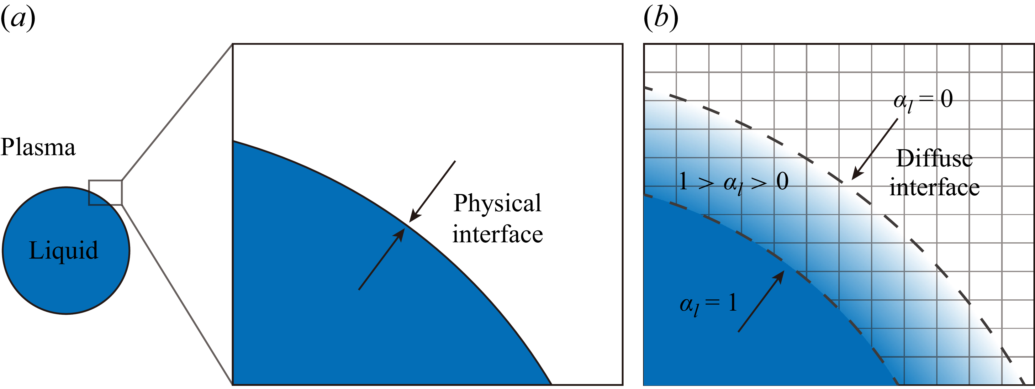
 a
a b
b αl
αl 0⩽αl⩽1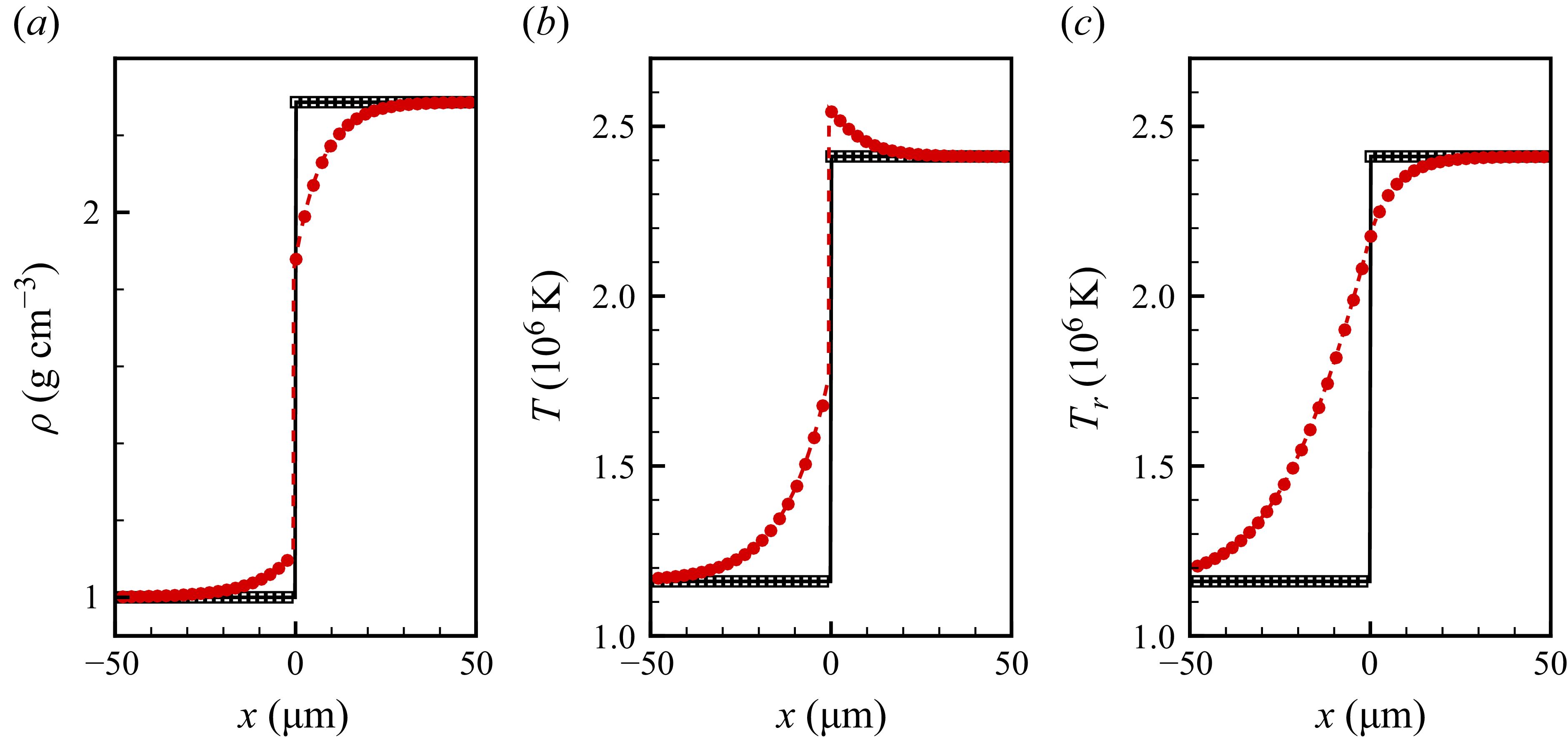
 0 ns
0 ns 4.2 ns
 8
8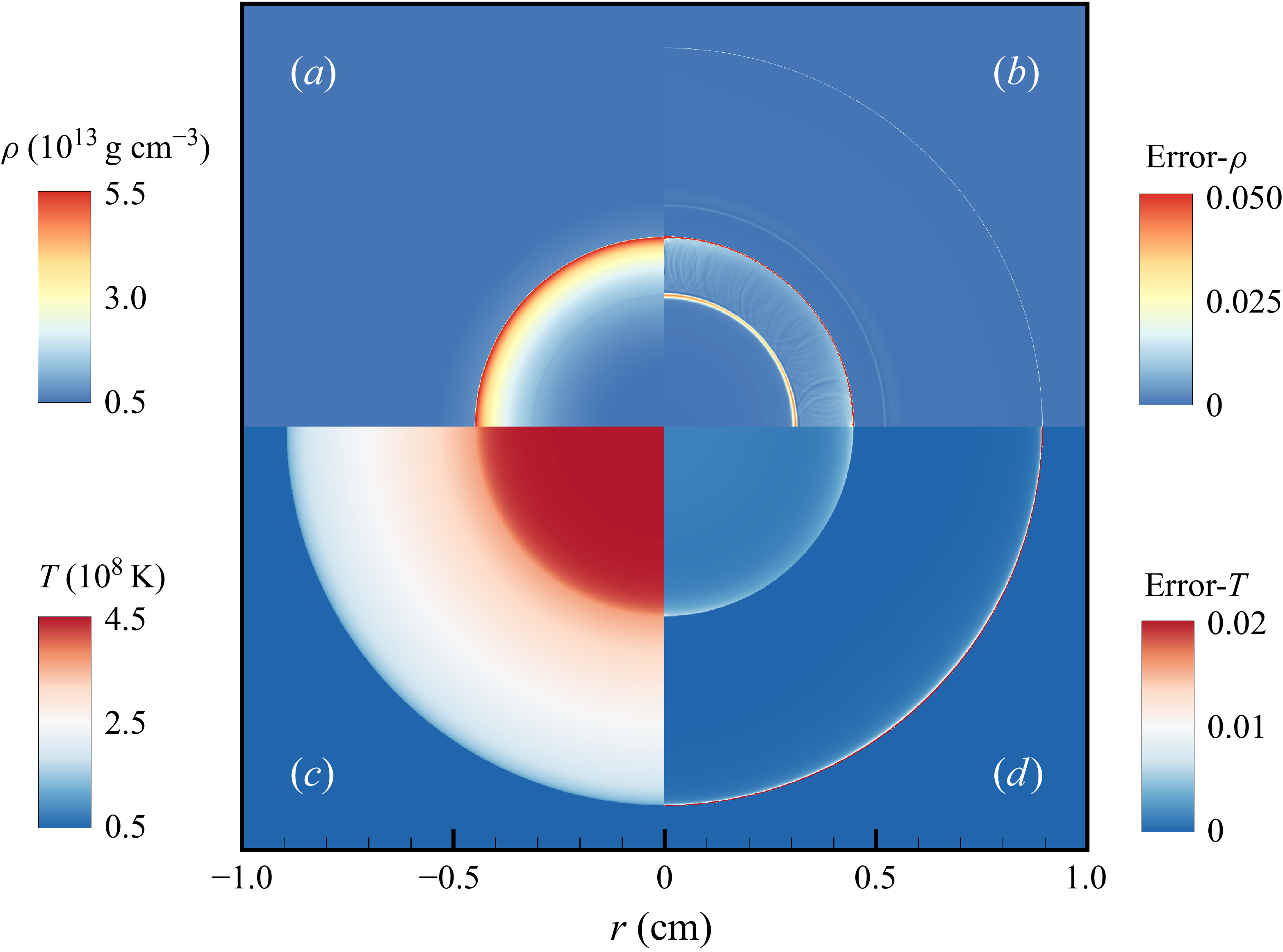
 |ρN−ρA|/ρA
 |TN−TA|/TA
 0.52 ns
 N
N A
A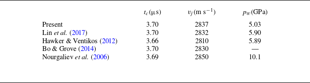
 tc
tc vj
vj pw
pw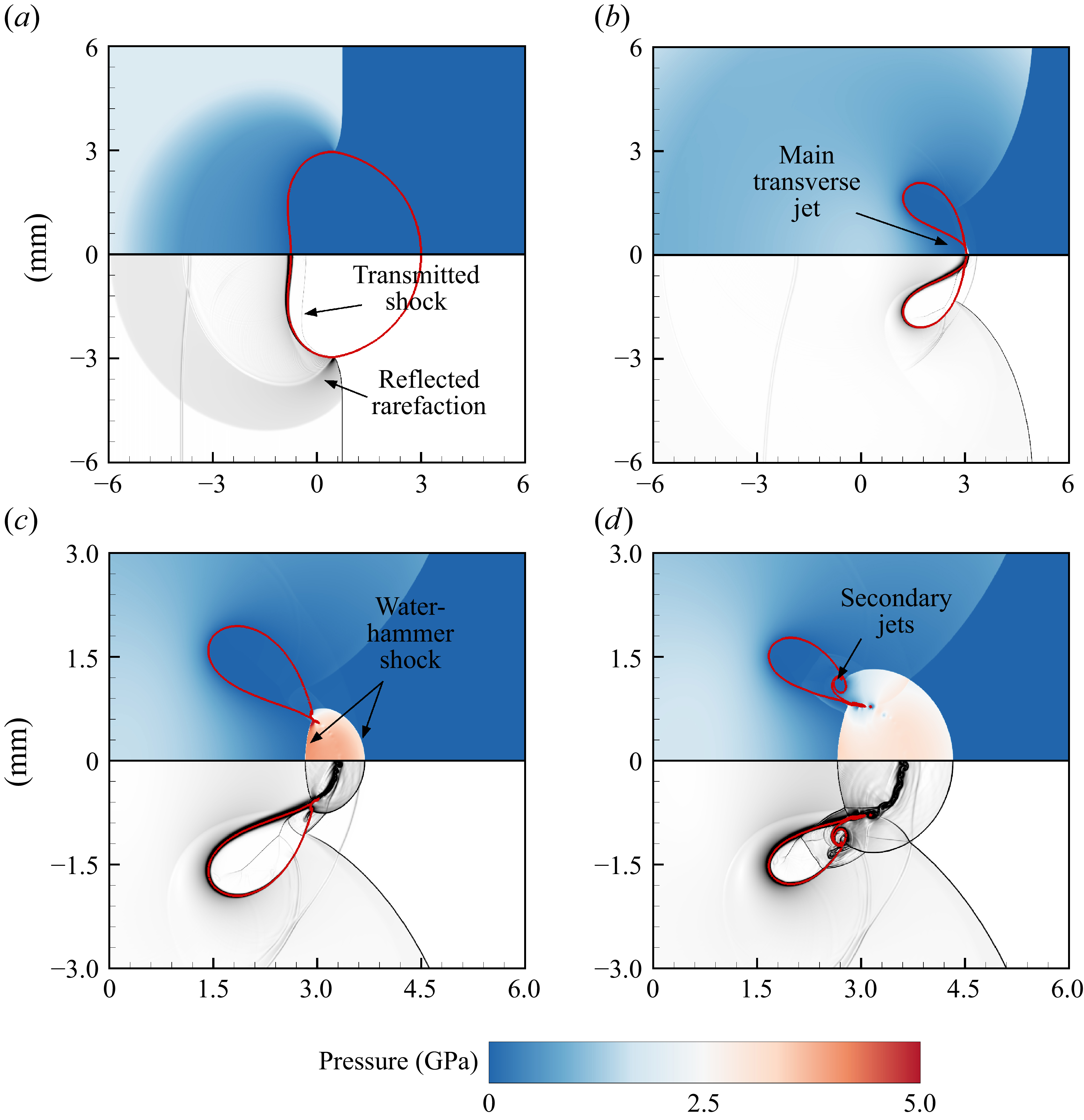
 2.2μs
2.2μs 3.7μs
3.7μs 3.9μs
3.9μs 4.1μs
4.1μs αg=0.5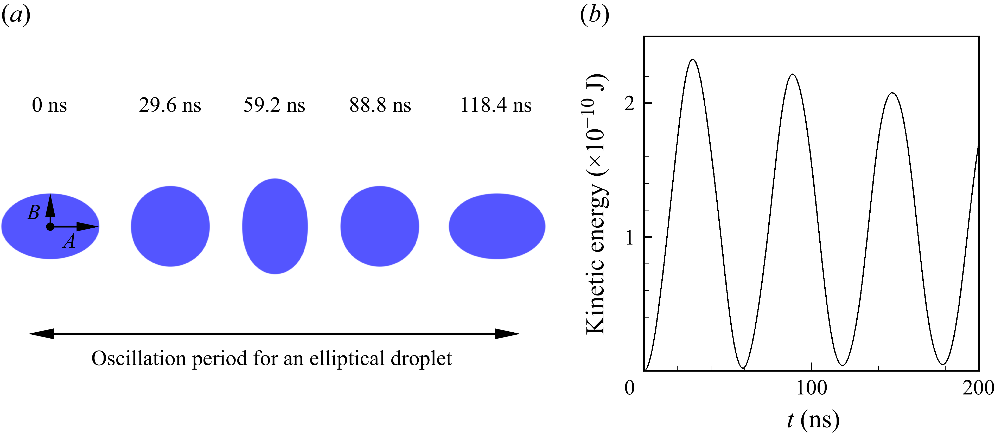
 a
a A
A B
B b
b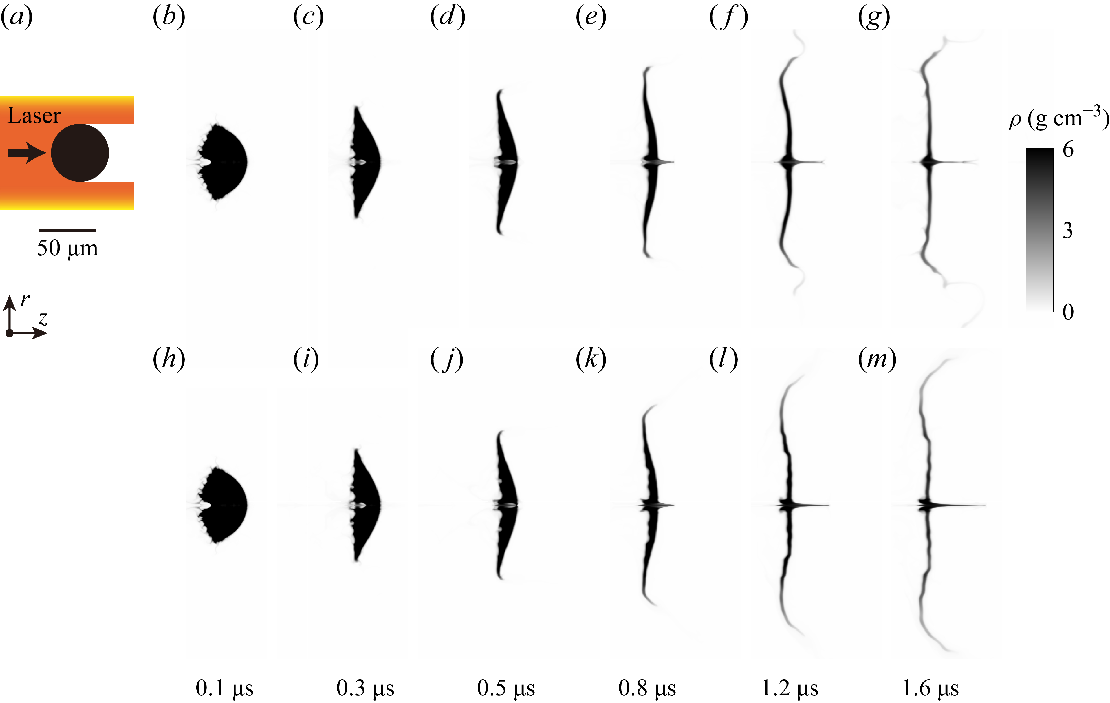
 a
a t=0.1 μs
 t=1.6 μs
 b
b g
g h
h m
m a
a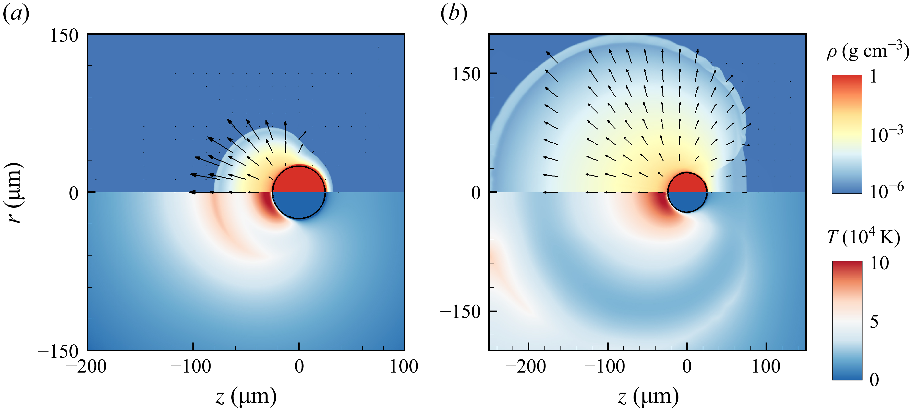
 a
a 2 ns
2 ns b
b 10 ns
10 ns αl=0.5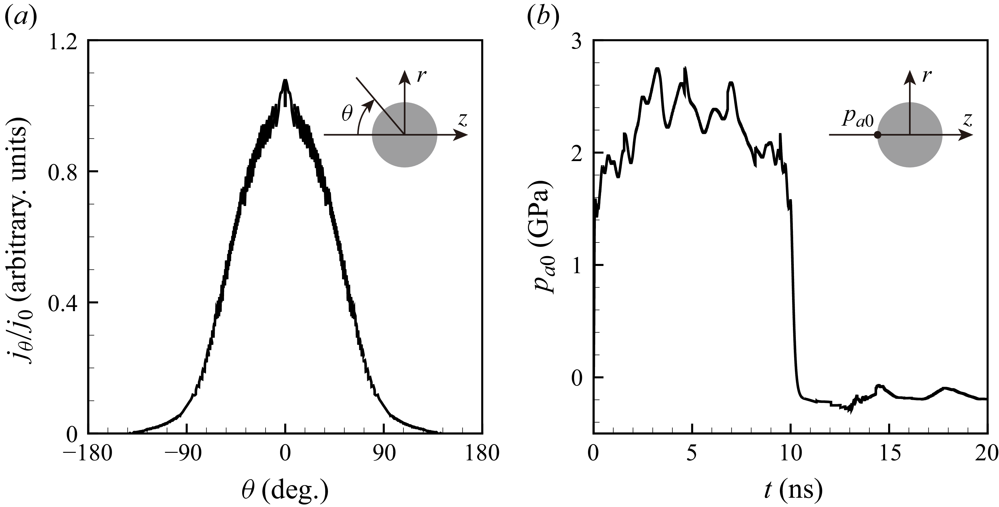
 a
a θ
θ r
r z
z b
b θ=0
θ=0 pa0
pa0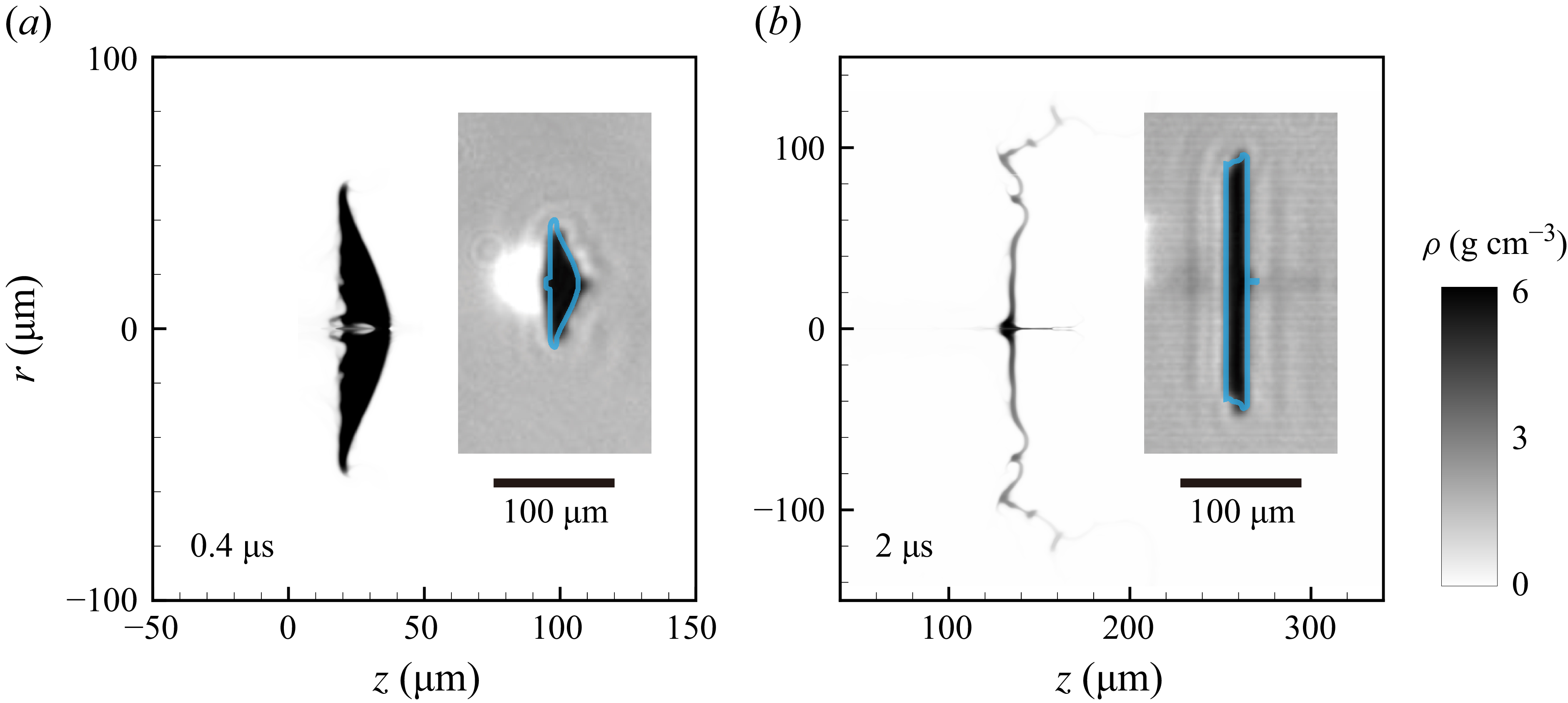
 a
a 0.4μs
0.4μs b
b 2μs
2μs ρ=1.2 gcm−3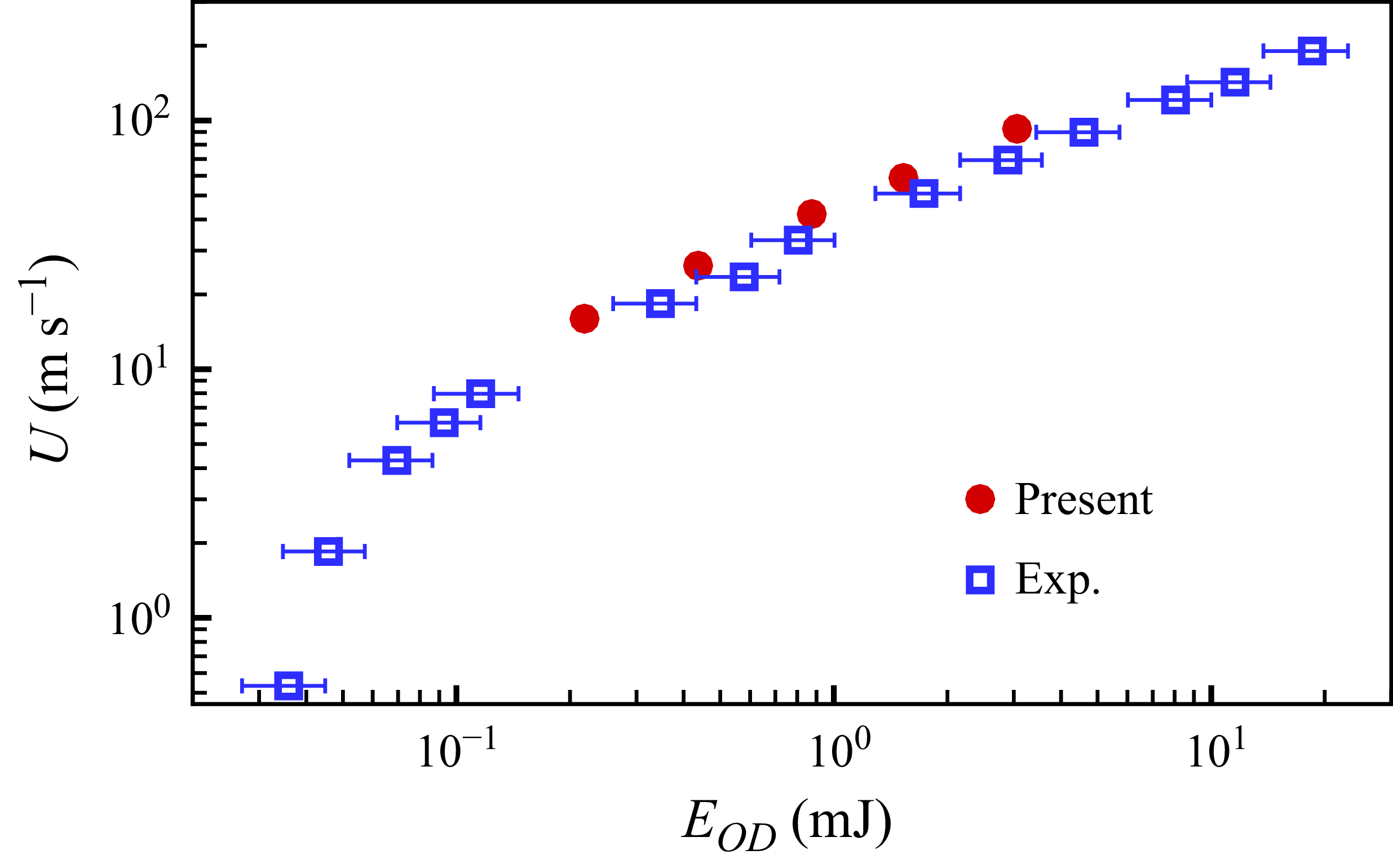
 U
U EOD
EOD a
a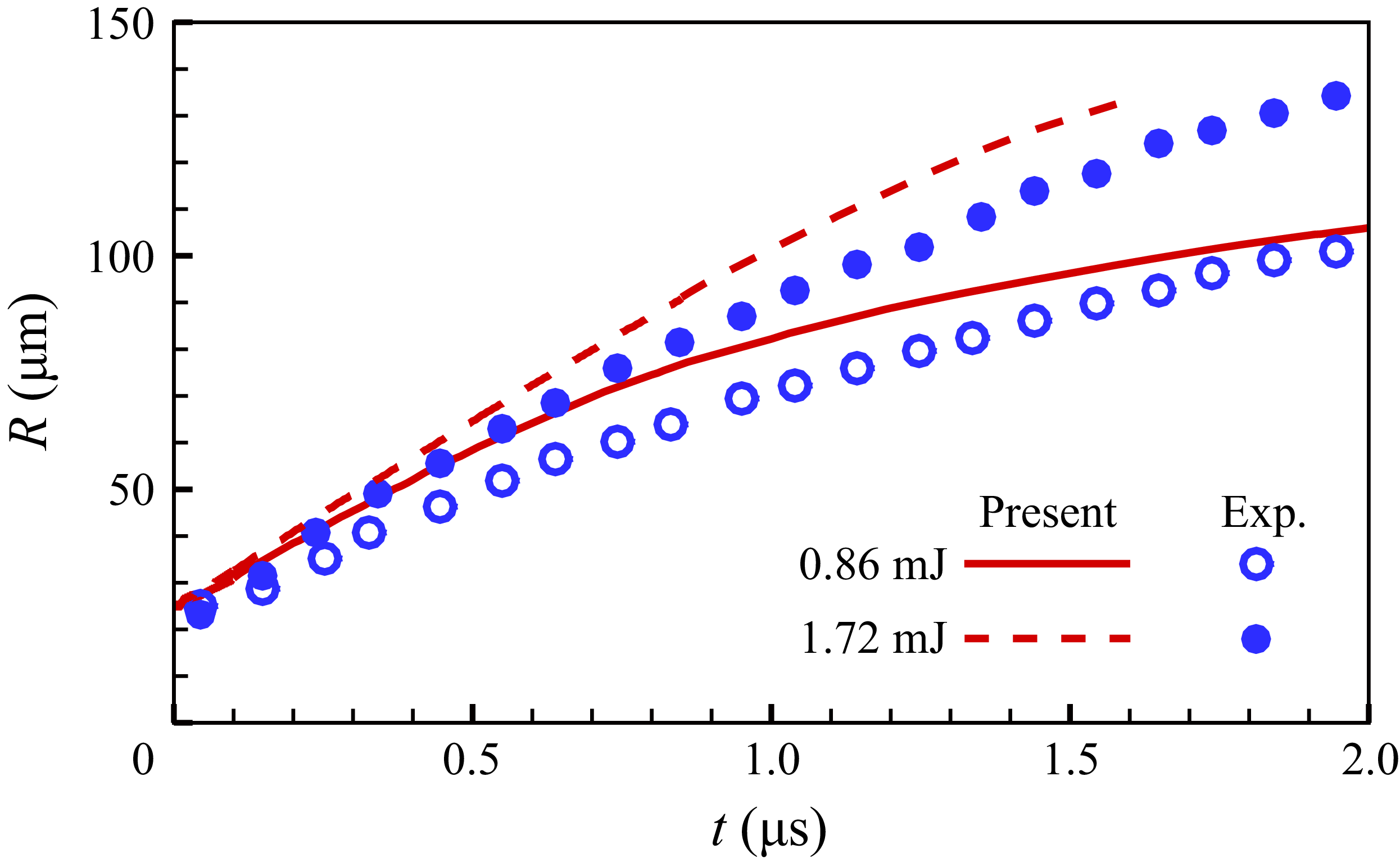
 EOD=0.86
 1.72 mJ
 a
a

