





1. Introduction
The advent of microfluidic devices has led to the development of microchip electrophoresis systems which enable rapid separation and detection of charged species from a small volume of sample mixture (Jacobson & Ramsey Reference Jacobson and Ramsey1995). Electrophoresis techniques are characterised by electrophoretic motion of ions and advection due to interfacially driven electroosmotic flow (EOF) (Levich Reference Levich1962) past the charged surface of the microchannel in the presence of an electric field. Microchip electrophoresis is often performed by incorporating a sample-stacking step wherein the sample mixed with low electrical conductivity electrolyte is introduced between two zones of high-conductivity electrolyte (Jacobson & Ramsey Reference Jacobson and Ramsey1995). The gradient in the local electric field associated with the conductivity gradient causes the sample ions to stack at the boundary of high- and low-conductivity zones prior to the separation, thereby improving the detection sensitivity (Bharadwaj & Santiago Reference Bharadwaj and Santiago2005; Dubey, Gupta & Bahga Reference Dubey, Gupta and Bahga2019).
A typical configuration of high- and low-conductivity electrolytes that is used for sample stacking in electrophoresis is illustrated in figure 1. Initially, a low-conductivity electrolyte is sandwiched between two zones of a high-conductivity electrolyte inside a microchannel, typically fabricated in glass. The high- and low-conductivity electrolytes are made by varying the acid and base concentrations in water. A strong external electric field is applied along the channel axis. The continuity of current in the channel results in the local electric field being higher and lower in the low- and high-conductivity regions, respectively. The axially varying electric field drives a fluid flow through two distinct mechanisms. Firstly, the axially varying electric field induces a non-uniform electroosmotic slip velocity at the channel walls due to the presence of immobile surface charges on the walls. In the absence of conductivity gradients, the bulk EOF driven by this electroosmotic slip velocity has a plug-shaped velocity profile (Levich Reference Levich1962). However, in the presence of streamwise conductivity gradients, the slip velocity is higher in the regions with low conductivity and lower in the high-conductivity regions, as depicted in figure 1. The non-uniform electroosmotic slip velocity induces internal pressure gradients to ensure continuity of flow and drives a recirculating flow over a mean flow that advects the conductivity field along the channel axis. The EOF driven by an inhomogeneous slip velocity at the channel walls (Anderson & Idol Reference Anderson and Idol1985; Ajdari Reference Ajdari1995) and its detrimental effects on electrophoretic separations due to sample dispersion have been studied extensively (Keely, van de Goor & McManigill Reference Keely, van de Goor and McManigill1994; Herr et al. Reference Herr, Molho, Santiago, Mungal, Kenny and Garguilo2000; Sounart & Baygents Reference Sounart and Baygents2001).
Schematic illustrating typical conductivity distribution required for sample-stacking step in microchip electrophoresis. Initially, a plug of low-conductivity electrolyte is surrounded by two high-conductivity electrolyte zones. An external electric field is applied along the axial direction. The axial gradients in conductivity lead to corresponding variations in the local electric field and the local electroosmotic slip velocity at the channel walls. The non-uniform electroosmotic slip velocity results in internal pressure gradients which lead to a non-uniform EOF.

Besides the interfacially driven EOF, the gradients in the local electric field accompanied by conductivity gradients can lead to instabilities in the flow (Hoburg & Melcher Reference Hoburg and Melcher1977; Baygents & Baldessari Reference Baygents and Baldessari1998; El Moctar, Aubry & Batton Reference El Moctar, Aubry and Batton2003; Chen et al. Reference Chen, Lin, Lele and Santiago2005; Posner & Santiago Reference Posner and Santiago2006; Gaur & Bahga Reference Gaur and Bahga2017; Sharan, Gupta & Bahga Reference Sharan, Gupta and Bahga2017). The electric field gradients lead to accumulation of free charge within the bulk fluid. In turn, this free charge couples with the local electric field to apply a destabilising electric body force on the fluid, which has the capability to induce an electrohydrodynamic instability. When such an instability appears in systems along with EOF, where EOF drives the fluid flow, the resulting instability is often termed an electrokinetic instability (EKI) (Chen et al. Reference Chen, Lin, Lele and Santiago2005; Ramos Reference Ramos2011). In microfluidic applications where significant mixing of fluids is desired, EKI is used as an active method for rapid mixing (Oddy, Santiago & Mikkelsen Reference Oddy, Santiago and Mikkelsen2001; Lin et al. Reference Lin, Storey, Oddy, Chen and Santiago2004; Dubey, Gupta & Bahga Reference Dubey, Gupta and Bahga2017). On the other hand, in microchip electrophoresis, such instabilities are undesirable as they can lead to the rapid dispersion of sample ions and deteriorate the separation performance (Ramsey Reference Ramsey2001; Lin Reference Lin2009).
Electrokinetic instabilities have been investigated experimentally and theoretically in various microchannel flow configurations, primarily for rapid mixing in low Reynolds number flows (Chen et al. Reference Chen, Lin, Lele and Santiago2005; Lin, Storey & Santiago Reference Lin, Storey and Santiago2008; Luo Reference Luo2009; Posner, Pérez & Santiago Reference Posner, Pérez and Santiago2012; Demekhin, Nikitin & Shelistov Reference Demekhin, Nikitin and Shelistov2013, Reference Demekhin, Nikitin and Shelistov2014; Dubey et al. Reference Dubey, Gupta and Bahga2017). However, EKI during sample stacking in electrophoresis (figure 1) is still not well characterised. Various studies of sample stacking in microchip electrophoresis have reported that large conductivity gradients in the presence of a strong electric field deteriorate the separation efficiency possibly due to EKI (Shultz-Lockyear et al. Reference Shultz-Lockyear, Colyer, Fan, Roy and Harrison1999; Dang et al. Reference Dang, Zhang, Jabasini, Kaji and Baba2003). The only conclusive report on EKI during sample stacking in microchip electrophoresis is that by Santos & Storey (Reference Santos and Storey2008), who performed numerical simulations of flow in a configuration similar to that shown in figure 1. Through simulations, Santos & Storey (Reference Santos and Storey2008) predicted recirculating flow in a frame of reference moving with the mean flow and the onset of instability above a threshold electric field. However, direct empirical evidence of the existence of such EKI has still not been reported. The key challenges in experimentally observing the EKI during sample stacking are the diffusive nature of the conductivity gradient, illustrated in figure 1, and the short time scale associated with EKI (Santos & Storey Reference Santos and Storey2008).
This paper presents a detailed experimental and numerical investigation of the EKI that occurs when a strong electric field is applied across a streamwise conductivity gradient in a microchannel, such as that during sample stacking in electrophoresis. We performed a series of controlled experiments involving high-speed imaging of a passive scalar for various electric field values to visualise this instability. Based on the analysis of experimental data, we report the dominant flow structures and the threshold criteria for the onset of instability. We supplement our empirical observations with numerical simulations to elucidate the physical mechanism underlying this instability. The experimental observations and simulation predictions clearly show that the instability results from the coupling of the electric field and the conductivity gradients set up by the non-uniform EOF.
The paper is structured as follows. Section 2 presents the experimental set-up and data analysis techniques. Section 3 presents the experimental observations. Sections 4 and 5 present the simulation approach and description of the physical mechanism of the instability through simulation results. The paper is then concluded in § 6 with remarks on the implications of the experimental and simulation results.
2. Experiments
2.1. Description of the flow
We performed experiments to visualise the EKI that sets in when a strong electric field is applied across a fluid in a microchannel with a streamwise gradient in electrical conductivity, as shown in figure 1. The schematic shown in figure 2 illustrates the two-step procedure that was devised to perform the experiments in a cross-shaped microchip. Figure 2(a) shows the injection step, wherein a low-conductivity ( $\sigma _L$) electrolyte is filled in the north (N) reservoir and a high-conductivity electrolyte ( $\sigma _H$) is filled in the west (W), east (E) and south (S) reservoirs. An electrically neutral fluorescent tracer, Rhodamine-B, is mixed in the high-conductivity electrolyte filled in the E channel to visualise the flow during experiments. In the first step, electric potential $V_1$ is applied at N and W reservoirs, and potential $V_2 >$ $V_1$ is applied at the E reservoir. This results in an EOF from the E, W and N reservoirs towards the cross-junction. The incoming fluid streams at the cross-junction flow towards the S reservoir, which serves as the sink. This flow configuration results in hydrodynamic focusing of the low-conductivity stream between two high-conductivity streams at the channel junction. The steady-state hydrodynamic focusing is achieved within one minute. Once a steady flow is achieved during the injection step, the interfaces between high- and low-conductivity zones in the main channel remain stationary at the cross-junction. This steady flow configuration results in a narrow plug of the low-conductivity electrolyte sandwiched between two adjacent zones of high-conductivity electrolytes. In the next step, the potentials at the channel ends are suddenly switched to generate an electric field that is collinear with the conductivity gradient, as shown in figure 2(b). Consequently, the EOF advects the low-conductivity plug into the main channel, connecting the cross-junction and the E reservoir. This results in a configuration similar to that depicted in figure 1. For the second step, the potentials applied at the N and S reservoirs are chosen so that the EOF in the vertical channels is minimised. No external pressure is applied at the channel ends, and all the reservoirs were maintained at atmospheric pressure. We tried various ways of visualising the flow by mixing the passive fluorescent tracer in other zones. As described later in § 4, the instability dynamics is primarily governed by the leading interface, due to which mixing the tracer in the leading high-conductivity zone provides the best visualisation of the instability.
Schematic illustrating the two-step procedure of experiment to visualise the EKI in a cross-shaped microchip. First, conductivity gradients are established by introducing a low-conductivity electrolyte from the north reservoir of the microchip and high-conductivity electrolytes from the east and west reservoirs. The electrolytes flow in the direction of the electric field in the respective channels. The flow is visualised by mixing Rhodamine-B dye with the high-conductivity electrolyte present in the east channel. Thereafter, upon switching the voltages at the reservoirs, the electric field in the main channel becomes colinear with the conductivity gradients. All the microchannels have a D-shaped cross-section with channel width  $w$ and depth $d$.
$d$.

2.2. Electrolyte solutions
The high- and low-conductivity electrolyte solutions were prepared upon diluting the stock solutions of 1 M each of MOPS (Sigma Aldrich, USA) and NaOH (CDH, India) using deionised water. The electrolyte having high conductivity consisted of 200 mM MOPS and 125 mM NaOH ( $\textrm {pH} = 7.3$). The measured electrical conductivity of the high-conductivity electrolyte was $\sigma _{H} = 0.51$ S m $^{-1}$. The low-conductivity electrolyte consisted of 20 mM MOPS and 10 mM NaOH ( $\sigma _{L} = 0.051$ S m $^{-1}$, $\textrm {pH} = 6.9$). The measured conductivity ratio ( $\gamma =\sigma _H/\sigma _L$) of these two electrolytes was 10. The viscosity and the permittivity of the electrolytes are assumed to be same as those of pure water due to the low concentration of electrolytes (Horvath Reference Horvath1985). To visualise the conductivity field in our experiments, the electrolyte solution with high conductivity was seeded with 0.5 mM Rhodamine-B which is reported to be electrically neutral for the pH values of the solution used in the experiments (Milanova et al. Reference Milanova, Chambers, Bahga and Santiago2011, Reference Milanova, Chambers, Bahga and Santiago2012). Because a neutral marker has negligible electrophoretic mobility, it does not interact with background electrolytes during the experiments. The values of various physical properties of the electrolyte are provided in table 1.
Properties of the electrolyte solutions and physical parameters of the microfluidic device.

2.3. Experimental set-up and image acquisition
All the experiments were conducted in a standard cross-shaped glass microchip (Micronit, The Netherlands) shown schematically in figure 2. The microchannels connecting the N, W and S reservoirs to the junction were 5 mm long, and the channel connecting the junction to the E reservoir was 35 mm long. All the channels had a D-shaped cross-section of width  $w=50 \mathrm {\mu }$m and depth $d=20 \mathrm {\mu }$m. Large reservoirs were attached to the channel ends to minimise variability due to evaporation, buffer depletion and unwanted pressure-driven flow due to the change in liquid level in the reservoirs during the experiments. A four-channel high voltage power supply (IONICS, India, max. 2 kV and 10 mA) was used to apply potential difference across the channels. Platinum wires were used as electrodes dipped into the reservoirs. The electric field direction in the channels was controlled by switching the electric potential at each reservoir using a computer-controlled relay switch. To visualise the scalar field, we used an inverted epifluorescence microscope (Nikon Eclipse Ti-U, Japan) equipped with a mercury arc lamp, $\times\,$20 objective (Plan Fluor, ELWD, $\textrm {NA}=0.45$), and Nikon G2-A filter set (510–560 nm bandpass excitation filter, 590 nm longpass barrier filter). The spatio-temporal evolution of the scalar concentration field was recorded using a Peltier-cooled high-speed sCMOS camera (Andor Zyla 5.5, UK).
For all the experiments, the image acquisition was started 1 s before applying the electric field to capture all the phases of the experiment. We acquired images of size  $2560 \times 150$ pixels which corresponds to $985 \times 58 \mathrm {\mu }$m physical area of the microfluidic chip. These snapshots were recorded at 572 f.p.s. for each experiment with an exposure of 1 ms. The data were also acquired at high frame rates of 650 and 850 f.p.s. and had similar spectral content, indicating the absence of aliasing.
Each snapshot of the scalar concentration field was corrected using a standard image correction method,
 \begin{gather} I(x,y)_{corrected}=\frac{I(x,y)_{raw}- \overline{I(x,y)_{bg}}}{\overline{I(x,y)_{ff}} -\overline{I(x,y)_{bg}}}, \end{gather}
 \begin{gather}\text{where}\quad \overline{I(x,y)}=\frac{\displaystyle\sum_{1}^{N} I(x,y)}{N}. \end{gather}
Here,  $I_{raw}$, $I_{ff}$ and $I_{bg}$ denote the raw, flat field and the background snapshots, respectively. The flat field images were obtained by filling all the channels uniformly with the electrolyte solution mixed with the fluorescent dye, whereas background images were captured by filling the electrolyte solution without the dye. This normalisation of pixel intensity was used to correct the raw signal for non-uniformity arising due to non-uniform illumination and the D-shape of the channel cross-section.
2.4. Experimental conditions
We conducted the experiments for six different electric field values in the range  $E = 10 - 60$ kV m $^{-1}$ while keeping the ratio of conductivity of electrolytes fixed at $\sigma _H/\sigma _L=10$. These values of the electric field are typical of those used in practical microchip sample stacking, which can vary between 10 and 100 kV m $^{-1}$ (Jacobson & Ramsey Reference Jacobson and Ramsey1995; Bharadwaj & Santiago Reference Bharadwaj and Santiago2005). The experiments were performed with an increment of ${\rm \Delta} E = 10$ kV m $^{-1}$ from an initial low electric field at which the flow is stable. In our work, we define the electric field as $E = (V_W-V_E)/L$, where $V_E$ and $V_W$ denote the potentials at E and W reservoirs, respectively, and $L=(L_E+L_W)$ denotes the sum of E and W channel lengths. Three repetitions of each experiment were performed on the same microfluidic chip to ensure repeatability of the phenomena. For the initial step of the experiment, shown in figure 2(a), we kept the same initial values of electric potentials ( $V_1=0.75$ kV and $V_2=1.45$ kV) at various reservoirs for all the experiments.
Before each experiment, all the microchannels were flushed sequentially with a 100 mM sodium hydroxide solution for 10 min and then using deionised water for another 10 min. After cleaning the microfluidic device, a fixed volume of  $25 \mathrm {\mu }$l of each electrolyte solution was filled in the respective reservoirs and vacuum was applied momentarily at S reservoir to fill all the channels. Subsequently, the electric potential was applied at various reservoirs to initiate the first step of hydrodynamically focusing the low-conductivity stream between two high-conductivity streams. We waited for over one minute to achieve steady hydrodynamic injection. Finally, at $t = 0$, the electric potential at each reservoir was switched in such a way that the low-conductivity zone moved further into the E channel, creating the configuration of collinear electric field and conductivity gradient, as shown in figure 2(b). Hence, at the beginning of the second step, at $t = 0$, the low-conductivity plug is at the channel junction. Later during the second step, the plug advects downstream of the E channel due to EOF.
2.5. Time scales and dimensionless numbers
The conductivity field in our experiments evolves due to advection and diffusion of electrolyte ions. Diffusion has a stabilising effect on the flow as it tends to diminish the conductivity gradients responsible for the instability. The time scale corresponding to the diffusion of the conductivity field is given by
 \begin{equation} \tau_{diff} \equiv \frac{w^2}{D_{eff}}, \quad \mbox{where } D_{eff}=\frac{2D_{+} D_{-}}{D_{+} + D_{-}}. \end{equation}
Here,  $D_{eff}$ is the effective diffusivity of the conductivity field (see § 4.1), $D_\pm$ denote the diffusivities of cations and anions of the electrolyte and $w$ is the width of the microchannel.
The fluid flow in the microchannel is driven by the electroosmotic slip at the channel walls with immobile surface charges and an electric body force that arises when an electric field is applied across a conductivity gradient. The electroosmotic slip velocity depends on the local tangential electric field  $E_t$ as (Hunter Reference Hunter1981; Probstein Reference Probstein2005)
 \begin{equation} u_{eof}={-}\frac{\epsilon \zeta E_t }{\eta} = \mu_{eof}E_t, \end{equation}
where 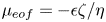 $\mu _{eof}= -\epsilon \zeta /\eta$ is termed the electroosmotic mobility of the channel surface. Here, $\epsilon$ is the permittivity of electrolyte, $\eta$ the dynamic viscosity and $\zeta$ the zeta-potential at the channel surface. For the system that we have considered in the current work, most of the main channel is filled with the high-conductivity electrolyte, as shown in figure 2(b). Therefore, the mean EOF velocity in the channel scales as $\mu _{eof} E$, where $E=(V_W-V_E)/(L_W + L_E)$ is the reference scale for the mean electric field in the channel. The corresponding time scale for advection due to EOF is given by
 \begin{equation} \tau_{eof} \equiv \frac{w}{\mu_{eof}E}. \end{equation}
 The instability is driven by an electric body force on the fluid that results from the coupling of electric field with the free charge in the regions with conductivity gradient. The appropriate reference scale for the resulting velocity, termed the electroviscous velocity  $U_{ev}$, is obtained by balancing the viscous and the electric body forces,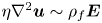 $\eta \nabla ^2\boldsymbol {u}\sim \rho _f \boldsymbol {E}$, where $\boldsymbol {u}$ denotes the velocity, $\rho _f$ the free charge density and $\boldsymbol {E}$ the local electric field. As shown by Hoburg & Melcher (Reference Hoburg and Melcher1976), from the continuity of current and Gauss's law, the free charge density is given by $\rho _f = \epsilon \boldsymbol {\nabla } \boldsymbol {\cdot }{\boldsymbol {E}} = -\epsilon \boldsymbol {E}\boldsymbol {\cdot } \boldsymbol {\nabla } \sigma / \sigma$ (see § 4.1). By balancing the viscous and the electric body forces, we arrive at the electroviscous velocity $U_{ev}$ and time scale $\tau _{ev}$,
 \begin{equation} U_{ev} \equiv\frac{\epsilon E^2 w}{\eta} \quad \mbox{and} \quad \tau_{ev}\equiv \frac{w}{U_{ev}}=\frac{\eta}{\epsilon E^2}. \end{equation}
Based on the values of various physical parameters of the electrolyte solutions and the microfluidic device given in table 1 and for a typical value of electric field  $E=30$ kV m $^{-1}$, the typical values of various time scales of the problem are: $\tau _{diff}=2.75$ s, $\tau _{eof}=32$ ms and $\tau _{ev}=1.6$ ms. For these experimental conditions, the time scale corresponding to the destabilising electroviscous velocity $(\tau _{ev})$ is significantly smaller than the time scale for diffusion $(\tau _{diff})$ which tends to stabilise the flow. Therefore, one can expect to observe an instability for these experimental conditions.
Besides the three time scales, ( $\tau _{diff}$, $\tau _{eof}$ and $\tau _{ev}$), the fluid flow in our experiments is governed by the geometric parameters of the device, ( $w$ and $d$), and the conductivity ratio ( $\gamma$). These six physical parameters can be grouped into the following four dimensionless numbers:
 \begin{equation} Ra_e \equiv \frac{\tau_{diff}}{\tau_{ev}}=\frac{\epsilon E^2 w^2}{\eta D_{eff}},\quad \frac{(\tau_{ev}\tau_{diff})^{1/2}}{\tau_{eof}}=\frac{-\zeta }{\sqrt{\eta D_{eff}/\epsilon}},\quad \frac{d}{w} \quad \mbox{and} \quad \gamma. \end{equation}
The dimensionless number  $Ra_e$, which is the ratio of time scales associated with diffusion and electrosviscous flow, is called the electric Rayleigh number (Chen et al. Reference Chen, Lin, Lele and Santiago2005; Posner & Santiago Reference Posner and Santiago2006; Dubey et al. Reference Dubey, Gupta and Bahga2017) which governs the onset of instability. In electrokinetic systems, the instability sets in at high $Ra_e$, when electroviscous flow amplifies the disturbances in the conductivity field faster than the rate at which diffusion dissipates these disturbances (Chen et al. Reference Chen, Lin, Lele and Santiago2005; Posner & Santiago Reference Posner and Santiago2006; Dubey et al. Reference Dubey, Gupta and Bahga2017). The second dimensionless number in (2.7a–d) can be interpreted as the dimensionless zeta-potential $-\zeta /\sqrt {\eta D_{eff}/\epsilon }$, which governs the ability of flow perturbations to convect with EOF against the dissipative effects (Chen et al. Reference Chen, Lin, Lele and Santiago2005). In the current work, we analyse the stability of electrokinetic flow by varying the electric field and hence the electric Rayleigh number. All other dimensionless numbers are kept constant in our experiments.
3. Experimental results
In this section, we present the features of the instability observed during the fluid flow. Experiments were performed to investigate the stable, onset of instability and unstable flow regimes by varying the electric field and correspondingly the electric Rayleigh number  $Ra_e$, which was calculated based on (2.7a–d) using the physical parameters listed in table 1. For these parameters, the conversion between electric field and Rayleigh number is $E = 0.724\sqrt {Ra_e}$ where the electric field is in kV m $^{-1}$. In figure 3, we present the time-resolved snapshots of the passive fluorescent tracer in the flow for $Ra_e= 760$, 4770 and 6870.
Instantaneous scalar concentration field recorded during experiments at three different electric Rayleigh numbers ( $Ra_e$). All the experiments have the same initial condition, wherein a low-conductivity zone is sandwiched between two high-conductivity zones. At $t = 0$, the voltages at the reservoirs are switched and the electric field in the main channel becomes colinear with the conductivity gradients. The low-conductivity plug is at the channel junction at $t = 0$, and later it advects downstream due to EOF. (a) The flow is stable at low electric field corresponding to $Ra_e=760$. (b) At a higher electric field, corresponding to $Ra_e= 4770$, an instability is observed. In particular, the high-conductivity electrolyte (dyed with fluorescent tracer) is drawn into the low-conductivity zone in the form of a narrow, oscillating stream. (c) At $Ra_e=6870$, the growth of instability is even faster. The instability at $Ra_e=4770$ and $6870$ is characterised by rapid dispersion of the conductivity gradient.

3.1. Stable flow
The evolution of flow at a low electric field value corresponding to  $Ra_e = 760$ is shown in figure 3(a). The region with conductivity gradients is comparatively small compared with the dimensions of the main channel. Therefore, here we present snapshots of a small region of $150 \mathrm {\mu }$m length and $50 \mathrm {\mu }$m width. Figure 3(a) shows the representative snapshots obtained at different time instants during the experiments. Note that the passive fluorescent tracer is purposely mixed in the high conductivity stream present on the right-hand side in the E channel to visualise the leading interface separating the high- and low-conductivity zones. Initially, a low-conductivity electrolyte plug is hydrodynamically focused between two high-conductivity streams at the channel junction, which results in a slanted conductivity interface at time $t=0$. For $Ra_e = 760$, the flow remains stable, and no perturbations in the concentration field of the passive scalar are observed. In figure 3(a), the interface separating the high- and low-conductivity regions on the right, as visualised by the passive scalar, can be seen advecting marginally downstream in the E channel due to EOF. Because the time scale over which the images were acquired was an order of magnitude smaller than the diffusion time scale ( $\tau _{diff}=2.75$ s), the conductivity gradient appears minimally diffused.
3.2. Unstable flow
A stable flow is observed in the experiments for electric Rayleigh numbers up to  $Ra_e= 1720$. Upon increasing $Ra_e$, the perturbations in the conductivity field, associated with the EKI, appear within the low-conductivity zone. To show the characteristics of the instability, we present the instantaneous snapshots of scalar concentration field at $Ra_e=4770$ and 6870, respectively in figure 3(b,c). The snapshots at $t=0$ are similar for all the experiments performed at different $Ra_e$ as the initial conditions are kept the same. For $Ra_e=4770$, figure 3(b) shows that the high-conductivity electrolyte seeded with the fluorescent tracer is drawn into the low-conductivity zone in the form of a thin stream. The high-conductivity stream oscillates in the spanwise direction and results in a rapid mixing within the low-conductivity region. Due to the instability, the dispersion of conductivity gradient occurs within ${\sim }10$ ms as opposed to the diffusion time scale of $\tau _{diff}\sim 2.75$ s.
As shown in figure 3(c), the instability sets in even earlier at higher  $Ra_e=6870$. The features of the instability appear similar to that at $Ra_e=4770$. The spanwise oscillations of the high-conductivity stream drawn into the low-conductivity region along with the advection of the conductivity gradient due to EOF result in alternating sequences of high- and low-conductivity zones (see figure 3c at $t=12$ ms). Due to the faster growth of instability at $Ra_e=6870$, the mixing of high- and low-conductivity streams is more uniform than that at $Ra_e=4770$. The instability fades away at a later time when the conductivity gradient disperses due to rapid mixing.
3.3. Proper orthogonal decomposition of experimental data
The instantaneous snapshots presented in figure 3 show that EKI in our experiments occurs for a short time duration before it fades away due to rapid dispersion of the conductivity gradients. We analysed the time-resolved snapshots of scalar concentration field using the proper orthogonal decomposition (POD) technique (Sirovich Reference Sirovich1987) to obtain the critical value of  $Ra_e$ for the onset of instability and to identify the dominant flow structures. The POD represents the spatio-temporal variation of any physical quantity ${v(\boldsymbol {x}},t)$ by a linear combination of spatially orthogonal modes $\psi _{i}(\boldsymbol {x})$ modulated by the time-dependent coefficients $a_{i}{(t)}$ as (Sirovich Reference Sirovich1987),
 \begin{equation} {v(\boldsymbol{x}},t)=\sum_{i=1}^{\infty} a_{i}{(t)} \psi_{i}(\boldsymbol{x}). \end{equation}
The spatial modes  $\psi _{i}(\boldsymbol {x})$ form an optimal basis, and they represent the coherent structures present in the flow.
We used the method of snapshots (Sirovich Reference Sirovich1987) to compute the POD of the scalar concentration field in our experiments. In this method, the time-resolved snapshots of the scalar field at every time instant are cast in the form for a vector  $\boldsymbol {v}_i$ and the data are represented in the form of a matrix ${\boldsymbol{\mathsf{V}}}$ as,
 \begin{equation} \boldsymbol{\mathsf{V}} = [\boldsymbol{v}_1, \boldsymbol{v}_2, \boldsymbol{v}_2,\ldots,\boldsymbol{v}_N], \end{equation}
where  $N$ denotes the total number of snapshots. The singular value decomposition of matrix ${\boldsymbol{\mathsf{V}}}$,
 \begin{equation} \boldsymbol{\mathsf{V}} = \boldsymbol{\mathsf{U}}\boldsymbol{\varSigma} \boldsymbol{\mathsf{W}}^{T}, \end{equation}
yields the POD of the data acquired at discrete time instants. The matrix  ${\boldsymbol{\mathsf{U}}}$ contains the orthogonal modes $\psi _{i}(\boldsymbol {x})$, whereas the matrix ${\boldsymbol{\mathsf{W}}}$ contains the time coefficients $a_i(t)$ of each mode. The diagonal elements of the diagonal matrix $\boldsymbol{\varSigma}$ are non-negative numbers $\textsf{$\mathit{\lambda}$}_i$, called the singular values, and are arranged in a descending order
 \begin{equation} {{\textsf{$\mathit{\lambda}$}^{(1)}}}\geq{{\textsf{$\mathit{\lambda}$}^{(2)}}}\geq,\ldots,{{\textsf{$\mathit{\lambda}$}^{(i)}}}\geq 0. \end{equation}
The amount of energy in the signal related to a given POD mode is directly proportional to the corresponding eigenvalue (Fukunaga Reference Fukunaga1990). Therefore, the ordering of eigenvalues according to (3.4) ensures that the POD modes are ranked in terms of their energy content. The relative contribution of the  $i$th POD mode to the total energy content of the flow is given by
 \begin{equation} \text{relative energy of } i^{\mathrm{th}} \text{ mode } = \frac{\textsf{$\mathit{\lambda}$}^{(i)}}{\displaystyle \sum_{k}{\textsf{$\mathit{\lambda}$}^{(k)}}}. \end{equation}
The onset of instability is identified when the number of dominant POD modes that capture 99 % of the total energy of the signal deviates significantly from the number of modes corresponding to the stable flow. The dominant flow structures also help in differentiating the unstable and stable flows. We performed POD analysis using  $N=25$ time-resolved snapshots of the fluorescent scalar field captured in every experiment. The data were analysed in a reference frame moving with the mean EOF velocity. To this end, we shifted the pixels in every snapshot by estimating the mean EOF velocity from the advection of the passive scalar. This resulted in a new set of snapshots wherein the conductivity gradient appears stationary and POD was performed on this set of images. Figure 4 shows the relative contribution of the first fifteen POD modes to the total energy content of the signal for $Ra_e=190 - 6870$. The singular values corresponding to dominant POD modes that cumulatively contribute to 99 % of the overall energy content of the signal are presented in table 2. For all values of $Ra_e$, the first POD mode is the most dominant mode with more than 90 % contribution to the total energy content of the signal. At $Ra_e=190$, the time-resolved snapshots have POD modes with only one dominant mode, as the flow is stable. Even at $Ra_e=760$, the energy contribution of the second POD mode is less than 1 %. At $Ra_e=1720$, a second mode with significant contribution appears in the flow, as shown in figure 4, suggesting the presence of instability. As $Ra_e$ is further increased, more dominant modes appear in the flow. At $Ra_{e} = 3050$ and 4770, there are three dominant modes that altogether sum up to 99 % of the total energy, whereas, at $Ra_{e} = 6870$, there are six most energetic modes.
The relative energy contribution of the first 15 POD modes at varying values of electric Rayleigh number ( $Ra_e$). At low values of $Ra_e = 190$ and 760, the first POD mode contributes approximately 99 % of the total energy of the signal. For $Ra_e= 1720$, the energy distribution shows significant deviation from that at lower $Ra_e$ values, indicating the presence of instability. At even higher $Ra_e$, a higher number of POD modes are dominant, corresponding to a stronger instability.

Relative energy of obtained POD modes for varying values of electric Rayleigh number.

We analysed the spatial POD modes for all  $Ra_e$ to identify whether the dominant POD modes correspond to coherent structures and not random experimental noise. In figure 5, we present the first seven spatial POD modes for $Ra_e=760$, 1720, 3050 and 6870. The first POD mode for all $Ra_e$ values is equivalent to the ensemble mean of the experimental snapshots, while the higher modes correspond to the fluctuations in the flow. At a low value of $Ra_e=760$, the second mode, which contributes less than 1 % to the total energy, shows localised fluctuations near the conductivity gradient. Comparing the POD modes with time-resolved snapshots in figure 3, it is evident that the second mode at $Ra_e=760$ corresponds to slight diffusion of the conductivity gradient in an otherwise stable flow. The third and higher POD modes at $Ra_e=760$ have significant experimental noise and they do not show meaningful coherent structures.
POD modes showing the coherent structures observed in experiments at different electric Rayleigh numbers  $(Ra_e)$. The flow is stable at low $Ra_e=760$, and only the first two modes are dominant. At $Ra_e = 1720$ and 3050, the flow is unstable, and the coherent structures appear throughout the low-conductivity zone. At very high value of $Ra_e= 6870$, the instability is stronger and is characterised by more energetic coherent structures.

At higher values of  $Ra_e = 1720$, 3050 and 6870, besides the dominant first mode, a large number of modes (modes 2 to 7) corresponding to different length scales of fluctuations are present. These modes show perturbations in the scalar concentration field throughout the low-conductivity zone, indicating the presence of an instability. In particular, mode 3 for $Ra_e = 1720$ and mode 2 for $Ra_e = 3050$ and 6870 clearly show the high-conductivity stream that is drawn into the low-conductivity electrolyte zone by non-uniform EOF. The higher modes are characterised by finer spatial structures with spanwise variations in the scalar concentration field. These modes correspond to the spanwise oscillations of the high-conductivity stream within the low-conductivity zone.
4. Numerical simulation
The experiments reported in § 3 provide conclusive evidence of EKI in a microchannel flow with streamwise conductivity gradients under an externally applied electric field. The instability occurs over a time scale of order 10 ms and measurements other than visualisation of a passive scalar in such a microfluidic system is rather challenging. Therefore, to gain a mechanistic understanding of the EKI phenomena, we performed numerical simulations of an electrokinetic system similar to that in the experiments. We begin this section by providing a brief description of the mathematical model and the numerical method used to simulate the instability. Subsequently, we present the simulation predictions at varying values of electric Rayleigh number  $(Ra_e)$.
4.1. Mathematical model
The flow velocity  $\boldsymbol {u}$ in an incompressible fluid flow driven by an electric field obeys the continuity equation,
 \begin{equation} \boldsymbol{\nabla} \boldsymbol{\cdot}{\boldsymbol{u}}=0. \end{equation}
The conservation of momentum is described by the Navier–Stokes equations with an additional electric body force term
 \begin{equation} \rho\frac{\partial \boldsymbol{u}}{\partial t}+\rho\boldsymbol{u}\boldsymbol{\cdot}\boldsymbol{\nabla} \boldsymbol{u} ={-}\boldsymbol{\nabla} p+\eta\nabla^2\boldsymbol{u}+ \rho_f \boldsymbol{E}. \end{equation}
Here  $\rho$, $p$ and $\eta$ denote the density, pressure and dynamic viscosity of the liquid, respectively. In this equation, $\rho _f{\boldsymbol {E}}$ is the electric body force which results from the coupling of the free charge density $\rho _f$ with the local electric field $\boldsymbol {E}$ in the fluid (Melcher & Schwarz Reference Melcher and Schwarz1968). We have retained the inertia terms in the momentum equation because the electroviscous velocity, defined by (2.6a,b), in our experiments corresponds to Reynolds number $Re = \rho U_{ev}w/\eta$ of $O(1)$. In particular, for a typical electric field of $E = 30$ kV m $^{-1}$, the electroviscous velocity from (2.6a,b) is $U_{ev}= 31~\mathrm {mm}$ s $^{-1}$, and $Re = 1.6$. Assuming that the electrolyte is a linear dielectric with spatially uniform dielectric permittivity $\epsilon$, the free charge density is given by Gauss’ law,
 \begin{equation} \rho_f=\epsilon \boldsymbol{\nabla} \boldsymbol{\cdot} \boldsymbol{E}.\end{equation}
The electric body force in (4.2) can therefore be expressed in terms of the local electric field as  $\rho _f{\boldsymbol {E}}=\epsilon (\boldsymbol {\nabla } \boldsymbol {\cdot } \boldsymbol {E})\boldsymbol {E}$.
The local electric field  $\boldsymbol {E}$ required to obtain the electric body force on the fluid depends on the spatial distribution of ions in the electrolyte. The transport of cations $(+)$ and anions $(-)$ in a binary electrolyte is governed by the electromigration–advection–diffusion equations,
 \begin{equation} \frac{\partial c_\pm}{\partial t}+ \boldsymbol{\nabla} \boldsymbol{\cdot} ({\boldsymbol{u}}c_\pm + \mu_+ c_\pm {\boldsymbol{E}} -D_\pm\boldsymbol{\nabla} c_\pm) =0. \end{equation}
Here,  $c$ denotes the ion concentration, $D$ the molecular diffusivity and $\mu$ the electrophoretic mobility. The diffusivity of ions is related to their electrophoretic mobility by Einstein's relation $D_\pm = \mu _\pm kT/(z_\pm e)$, where $k$ is the Boltzmann constant, $T$ the absolute temperature and $e$ the elementary charge. The above set of transport equations can be simplified by assuming that the electrolyte solution is approximately electroneutral, $z_+ c_+ \simeq -z_- c_-$ (Levich Reference Levich1962; Chen et al. Reference Chen, Lin, Lele and Santiago2005). Multiplying the transport equations (4.4) for cations and anions with $z_\pm F$ ( $F$ is the Faraday constant) and summing them up, while invoking the electroneutrality assumption, yields
 \begin{equation} \boldsymbol{\nabla} \boldsymbol{\cdot} (\sigma \boldsymbol{E} - \boldsymbol{\nabla} S )= 0, \quad S=z_+ D_+ c_+ F + z_ -D_- c_- F, \end{equation}
where  $\sigma =(z_+\mu _+ c_+ + z_-\mu _- c_-) F$ is the electrical conductivity of the electrolyte. Equation (4.5) describes the conservation of total current which is the sum of ohmic current $\sigma \boldsymbol {E}$ and the diffusion current $-\boldsymbol {\nabla } S$. As shown by Chen et al. (Reference Chen, Lin, Lele and Santiago2005), typically for a strong electric field of ${O}(10 \mbox {kV m}^{-1})$ such as that in our experiments, the ohmic current is significantly larger than the diffusion current. Therefore, the diffusion current can be neglected and (4.5) simplifies to Ohm's law,
 \begin{equation} \boldsymbol{\nabla} \boldsymbol{\cdot} (\sigma \boldsymbol{E})= 0.\end{equation}
 The governing equation for conductivity  $\sigma$ is derived by multiplying the transport equations (4.4) for cations and anions with $z_\pm \mu _\pm F$ and by adding the two equations. Eliminating the electric field $\boldsymbol {E}$ from the resulting equation using (4.5) and using the electroneutrality assumption leads to a convection–diffusion equation for the conductivity field,
 \begin{equation} \frac{\partial\sigma}{\partial t}+{\boldsymbol{u}}\boldsymbol{\cdot}\boldsymbol{\nabla} \sigma = D_{eff} \nabla^{2}\sigma, \quad D_{eff}=\frac{(z_+-z_-) D_+D_-}{z_+D_+-z_-D_-}. \end{equation}
For a binary electrolyte having ions with valences  $z_+=-z_-$, the effective diffusivity is given by $D_{eff}=2D_+D_-/(D_+ + D_-)$. Lastly, due to the low current density and displacement current in electrokinetic flows, the electric field can be assumed to be quasistatic and hence irrotational,
 \begin{equation} \boldsymbol{\nabla} \times \boldsymbol{E}=0. \end{equation}
Therefore, the electric field is related to the electric potential  $\phi$ by $\boldsymbol {E}=-\boldsymbol {\nabla } \phi$.
Equations (4.1)–(4.3), (4.6)–(4.8) describe the electric field-driven flow in an electrolyte with conductivity gradients. Note that in the derivation of these governing equations, we have used the electroneutrality assumption for mass conservation of ions but included an electric body force due to free charge in the momentum equation (4.2). This is due to the fact that the conductivity variation leads to gradients in the local electric field which in turn lead to accumulation of free charge in the fluid. The difference in the concentration of cations and anions associated with this accumulated free charge is small compared with the bulk ion concentrations, therefore it can be ignored for mass conservation. However, the coupling of a small amount of charge with a strong electric field results in an appreciable electric body force that cannot be neglected (Hoburg & Melcher Reference Hoburg and Melcher1977; Ramos Reference Ramos2011). Therefore, for a given conductivity field, we use Ohm's law (4.6) to solve for the electric field, which is then used to determine the free charge density  $\rho _f$ from Gauss’ law (4.3). The free charge density is therefore given by
 \begin{equation} \rho_f=\epsilon \boldsymbol{\nabla} \boldsymbol{\cdot} \boldsymbol{E}={-}\epsilon \boldsymbol{E}\boldsymbol{\cdot} \boldsymbol{\nabla} \sigma/\sigma.\end{equation}
This equation clearly shows that free charges are induced in the regions with conductivity gradients (Wang, Yang & Zhao Reference Wang, Yang and Zhao2016).
We solved the governing equations in a two-dimensional computational domain, shown schematically in figure 6. We choose the following reference scales to non-dimensionalise the governing equations:
 \begin{equation} \left.\begin{array}{c@{}} {[}x,y]=w,\quad [\phi] = \phi_0,\quad {[}\boldsymbol{E}]=E_0 =\dfrac{\phi_0}{L},\quad {[}\boldsymbol{u}]=U_{ev}=\dfrac{\epsilon E_0^2w}{\eta},\\ {[}t]=\dfrac{w}{U_{ev}},\quad [p]=\epsilon E_0^2,\quad [\sigma]=\sigma_L. \end{array}\right\} \end{equation}
Here,  $\phi _0$ is the voltage difference applied across the channel and $L$ is the channel length, as shown in figure 6. This scaling yields the following set of non-dimensionalised governing equations:
 \begin{gather} \boldsymbol{\nabla} \boldsymbol{\cdot}{\boldsymbol{u}}=0, \end{gather}
 \begin{gather}\frac{Ra_e}{Sc}\frac{\textrm{D} \boldsymbol{u}}{\textrm{D} t} ={-}\boldsymbol{\nabla} p + \nabla^2\boldsymbol{u}+ \nabla^2\phi \boldsymbol{\nabla} \phi, \end{gather}
 \begin{gather}\boldsymbol{\nabla} \boldsymbol{\cdot}(\sigma\boldsymbol{\nabla} \phi)=0, \end{gather}
 \begin{gather}\frac{\textrm{D}\sigma}{\textrm{D} t} = \frac{1}{Ra_e}\nabla^{2}\sigma. \end{gather}
Here,  $Ra_e$ is the electric Rayleigh number, and $Sc$ is the Schmidt number defined as
 \begin{equation} Ra_e=\frac{\epsilon E_0^2 w^2}{\eta D_{eff}}\quad\mbox{and}\quad Sc=\frac{\eta}{\rho D_{eff}}. \end{equation}
Sketch of the two-dimensional computational domain showing various geometric parameters and boundary conditions. A low-conductivity zone with a length equal to the channel width is initially surrounded by two high-conductivity electrolyte zones. The length and the width of the computational domain are the same as those of the microchip used in the experiments. The encircled numbers refer to the boundaries of the model geometry. The boundary conditions corresponding to these numbers are described in detail in table 3.

4.2. Initial and boundary conditions and numerical method
The initial and boundary conditions used to simulate the EKI are depicted in the schematic of the computational domain in figure 6. Initially, a plug of low-conductivity electrolyte is surrounded by two zones of high-conductivity electrolyte. In the beginning, the flow configuration remains stationary as no potential difference is applied across the channel. At  $t=0$, a potential difference $\phi _0$ is applied which drives fluid flow in the microchannel. The physical dimensions of the channel and the low-conductivity plug in the simulations were the same as those in the experiments. In this work, the experiments were designed to ensure negligible flow in the N and S channels of the microfluidic device (figure 2). Therefore, N and S channels were not included in the computational domain.
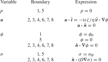
The boundary conditions used in the simulations are summarised in table 3. The inlet and the exit of the channel are maintained at the same pressure  $p=0$. The tangential electroosmotic slip boundary condition (2.4) is imposed on the impermeable channel walls to model the EOF. No flux boundary conditions for conductivity and electric field are applied on the channel walls. The conductivity at the channel ends is kept fixed at $\sigma _H$. The conductivity of the electrolyte solutions in the simulations is the same as those of electrolytes used in the experiments. The values of various physical parameters used for the simulations are provided in table 1. The value of zeta-potential ( $\zeta = - 74.7$ mV) used in the electroosmotic slip boundary condition (2.4) was estimated using the current monitoring method (Babar, Dubey & Bahga Reference Babar, Dubey and Bahga2020) . For this value of zeta-potential and transverse channel dimensions of order $10 \mathrm {\mu }$m, the Bikerman number, defined as $Bi = \delta \, \textrm {e}^{|ze\zeta /kT|/2}$, is negligible ( $Bi\ll 1$), where $\delta$ is the ratio of electric double layer (EDL) thickness to the characteristic width of the microchannel (Schnitzer & Yariv Reference Schnitzer and Yariv2012). In this $Bi\ll 1$ limit, surface conduction through the EDL (Bikerman Reference Bikerman1940; O'Brien & Hunter Reference O'Brien and Hunter1981) can be neglected. Therefore, the only effect of the EDL is to provide an electroosmotic slip velocity at the channel walls. Note that we have chosen the channel dimensions and the boundary conditions to be the same as those in the experiments to validate our simulations. In this respect, our simulations are more realistic than the EKI simulations in a periodic domain presented by Santos & Storey (Reference Santos and Storey2008). The periodic boundary conditions cannot be realised in experiments, and hence the simulations of Santos & Storey (Reference Santos and Storey2008) cannot be directly verified with experimental observations.
Boundary conditions corresponding to the computational domain shown in figure 6.
The governing equations described in § 4.1, along with the above mentioned initial and boundary conditions, were solved numerically using a commercial simulation package, COMSOL Multiphysics (COMSOL AB, Stockholm, Sweden), which is based on the finite element method. We implemented the governing equations and the associated initial and boundary conditions using the solver's in-built laminar flow and partial differential equation (PDE) modules. We used the laminar flow module to incorporate the continuity and momentum equations and used the PDE module to incorporate the governing equations for electric field and electrolyte conductivity. The choice of COMSOL package was based on its capability to accurately simulate chaotic electrokinetic flows involving a wide range of spatio-temporal scales (Karatay, Druzgalski & Mani Reference Karatay, Druzgalski and Mani2015). An unstructured grid of triangular elements is used to discretise the computational domain. To reduce the computational time, we use a coarse grid everywhere except in a small region surrounding the low-conductivity zone,where a fine mesh has been employed. The coarse mesh has a uniform element size of  $10 \mathrm {\mu }$m, whereas the fine mesh has a minimum and maximum element size of $0.4 \mathrm {\mu }$m and $1 \mathrm {\mu }$m, respectively. A time-dependent multifrontal massively parallel sparse direct solver is employed for transient calculations. The time stepping is performed using a second-order implicit backward difference scheme.
5. Simulation results
We performed simulations at various electric fields ( $\phi _0/L$) in the range $10 - 30 \textrm {kV} \textrm {m}^{-1}$ while keeping the conductivity ratio fixed at $\gamma =10$. In terms of dimensionless numbers, the electric Rayleigh number $Ra_e$ is varied by varying the electric field, while $Sc$ and $\gamma$ are kept fixed. For consistency, we have used the same definition of $Ra_e$ for presenting the simulation and experiment results. In contrast to the experiments, the simulations are two-dimensional wherein viscous stresses due to velocity gradients in the depth direction are absent. Therefore, we expect the simulations to predict instability at lower values of $Ra_e$ compared with that in the experiments.
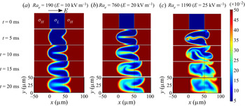
We begin by presenting the qualitative features of instability predicted by the simulations at various electric field values (or electric Rayleigh numbers  $Ra_e$). Figure 7 shows the time evolution of scalar conductivity field predicted by the simulations at three different electric fields of 10, 20 and 25 kV m $^{-1}$, corresponding to $Ra_e = 190$, 760 and 1190. Initially, the low-conductivity zone is surrounded by two regions of high-conductivity electrolyte. Thus, two sharp interfaces exist initially between the high- and low-conductivity regions. At $t=0$, an external electric field pointing from the W to E ends of the channel is applied. At low $Ra_e=190$, the simulation predicts that the flow is stable, but the non-uniform EOF associated with the heterogeneous electrolyte conductivity deforms the conductivity gradients. As shown in figure 7(a), the non-uniform EOF draws the high-conductivity electrolyte present on the right into the low-conductivity zone. Consequently, the initially straight interface between the high- and low-conductivity zones on the right deforms into a triangular shape. However, due to a relatively low electric field, the conductivity field remains symmetric across the channel centreline and diffuses over time without exhibiting any instability.
Representative snapshots showing simulated evolution of conductivity field with time for varying electric Rayleigh numbers  $Ra_e$. The high-conductivity regions are shown in red colour and the low-conductivity regions are shown in blue colour. (a) At low $Ra_e=190$, the flow remains stable, and a thin stream of high-conductivity electrolyte is drawn into the low-conductivity zone due to non-uniform EOF. (b) At an increased value of $Ra_e= 760$, an instability sets in and the stream of high-conductivity electrolyte within the low-conductivity electrolyte shows asymmetric fluctuations. (c) The instability becomes more chaotic at $Ra_e = 1190$, and it fades out over time due to the rapid dispersion of conductivity gradients. The instability is confined to the low-conductivity zone and lasts for a short time duration of order 20 ms.

Figure 7(b) shows the spatio-temporal evolution of the conductivity field at a higher electric field of 20 kV m $^{-1}$ corresponding to $Ra_e=760$. In this case, the leading interface separating the high- and the low-conductivity zones deforms faster due to non-uniform EOF. At $t=5$ ms, a thin stream of high-conductivity electrolyte is drawn into the low-conductivity zone. This results in a configuration wherein the conductivity gradients within the low-conductivity plug become orthogonal to the electric field. At a later time, an instability is observed within the low-conductivity zone, which resembles the EKI in microchannel flow with an orthogonal conductivity gradient and electric field (Posner & Santiago Reference Posner and Santiago2006; Dubey et al. Reference Dubey, Gupta and Bahga2017). The instability is characterised by asymmetric oscillations of the thin stream of high-conductivity electrolyte within the low-conductivity plug, as was also observed in the experiments. At an even higher electric field of 25 kV m $^{-1}$ ( $Ra_e=1190$), figure 7(c) shows that the unstable motion appears more chaotic. In particular, once the instability sets in, the high-conductivity electrolyte is drawn into the low-conductivity zone at various locations on the leading interface. The chaotic flow leads to rapid mixing within the low-conductivity zone. Note that the instability is confined to the low-conductivity zone, where strong local electric field and conductivity gradients lead to a destabilising electric body force on the fluid. The instability features predicted by the simulation are qualitatively similar to those observed in the experiments, described earlier in § 3. Simulations and experiments show that the instability sets in within a few milliseconds and lasts for a time duration of order 20 ms. This can be attributed to the fact that the time scale corresponding to the destabilising electroviscous flow is $\tau _{ev} = 1.6$ ms for an electric field of 30 kV m $^{-1}$. The flow instability causes rapid mixing of high- and low-conductivity zones within a short time duration, and the instability fades away when the conductivity gradients diminish. Thereafter, the dispersed low-conductivity plug slowly advects along the main channel due to EOF over a time scale of $\tau _{eof}=32$ ms and simultaneously diffuses into the adjoining high-conductivity zones over a time scale of $\tau _{diff}= 2.75$ s.
5.1. The role of electric body force and physical mechanism of instability
Having discussed the qualitative features of the instability through the evolution of the conductivity field, we now discuss the role of the electric body force in destabilising the microchannel flow and the physical mechanism of instability. In figures 8 and 9 we present the simulated time evolution of the conductivity field, free charge, electric field and the streamlines of flow for  $Ra_e=190$ and 1190, respectively. At the low electric field corresponding to $Ra_e=190$, the conductivity and the flow fields remain symmetric about the centreline of the channel for all times, as shown in figure 8. The non-uniform electroosmotic slip velocity at the channel walls due to streamwise conductivity gradients results in two large symmetric vortices in the low-conductivity region. This recirculating fluid motion draws the high-conductivity electrolyte into the low-conductivity region.
Simulated evolution of the conductivity field, free charge density, electric field and streamlines for electric Rayleigh number  $Ra_e = 190$. For better visualisation, a small part ( $150 \mathrm {\mu }\textrm {m} \times 50 \mathrm {\mu }\textrm {m}$) of the computational domain is shown here. (a) The temporal evolution of the conductivity field shows that the flow remains stable at low electric field. The flow recirculation draws in the high-conductivity electrolyte into the low-conductivity zone. (b) The free charge is induced in the regions with conductivity gradients and this charge couples with the local electric field to apply a body force on the fluid. At $Ra_e = 190$, the body force is not strong enough to destabilise the flow. (c) Consequently, the flow remains symmetric about the centreline as depicted by the streamlines.

Simulated conductivity field, free charge density, electric field and flow field for  $Ra_e=1190$. (a) Instability at high $Ra_e$ leads to rapid mixing of high- and low-conductivity solutions. The instability is characterised by an asymmetry in charge distribution and electric field as shown in (b) and asymmetric vortices as shown by the streamlines in (c). During the initial phase of the instability ( $t=2$ ms), the high-conductivity solution is drawn into the low-conductivity zone. The high-conductivity stream within the low-conductivity zone gets disturbed ( $t=5$ ms) and leads to a redistribution of charge and local electric field. The resulting electric body force drives a flow which further amplifies the disturbances.

As shown in figure 8(b), a negative (positive) free charge is induced in the regions with conductivity gradients, where the electric field points from low (high) to high (low) conductivity regions. The electric body force on the fluid acts only in the regions with free charge. At  $Ra_e=190$, the electric body force is not strong enough to produce sufficiently high electroviscous velocity to destabilise the flow. Therefore, the flow remains symmetric about the centreline, and the conductivity gradients diffuse over time.
At the high electric field corresponding to  $Ra_e = 1190$, the flow recirculation is stronger, and it quickly draws the high-conductivity electrolyte into the low-conductivity plug, as shown in figure 9. Consequently, within the low-conductivity plug, a new configuration is created wherein a high-conductivity stream flows between two adjoining streams of low-conductivity and the conductivity gradient is orthogonal to the electric field. This flow configuration resembles that in electrokinetic mixers wherein a high-conductivity stream flowing between two low-conductivity sheath streams destabilises upon applying a high axial electric field (Posner & Santiago Reference Posner and Santiago2006; Dubey et al. Reference Dubey, Gupta and Bahga2017). EKI in this flow configuration has been widely studied through experiments (Posner & Santiago Reference Posner and Santiago2006; Dubey et al. Reference Dubey, Gupta and Bahga2017) and simulations (Li, Delorme & Frankel Reference Li, Delorme and Frankel2016). Therefore, after the high-conductivity electrolyte is drawn into the low-conductivity plug by the recirculatory flow, the flow destabilises due to the same physical mechanism as in electrokinetic mixing experiments of Posner & Santiago (Reference Posner and Santiago2006). The symmetric vortices at early times ( $t=2$ ms) give way to asymmetric vortices associated with the instability ( $t=5$ ms and later). The instability further deforms the conductivity gradients and establishes an intricate flow pattern characterised by more than two eddies.
The destabilising nature of the electric body force can be understood from the simulation predictions at  $t=2$ and $5$ ms in figure 9. At $t=2$ ms, a high-conductivity stream is drawn into the low-conductivity plug. From (4.9) it is evident that a negative (positive) charge is induced in the region where the local electric field has a component that points from the low (high) conductivity region to the high (low) conductivity region. Consequently, as shown in figure 9(b) at $t=2$ ms, a negative charge is induced on the interface of the high-conductivity stream within the low-conductivity plug. Any disturbance of this high-conductivity stream leads to a change in the charge distribution at the interface of the stream, as observed at $t=5$ ms in figure 9. The free charge at the interface of the high-conductivity stream couples with the local electric field and drives an electroviscous flow which further amplifies the disturbance in the conductivity field, as shown by the streamlines. For example, the high-conductivity stream is perturbed downwards at point A and upwards at point B at $t=5$ ms in figure 9. This disturbance causes a body force that drives a downward flow at A and upward flow at B, further amplifying the disturbance. Consequently, the instability is characterised by a wavy structure of the high-conductivity stream within the low-conductivity plug. Similar wavy structures have been observed in EKI in a different microchannel flow configuration with orthogonal conductivity gradient and electric field (Dubey et al. Reference Dubey, Gupta and Bahga2017). At such high $Ra_e$, the electroviscous flow is strong enough to amplify the disturbances in the conductivity field faster than the rate at which conductivity gradients diffuse, resulting in the instability. The instability is localised in the low-conductivity plug because the local electric field is an order of magnitude greater as compared with that in the high-conductivity region attributed to the conductivity ratio $\gamma = \sigma _H/\sigma _L$.
To further highlight the role of electric body force in destabilising the flow, we performed an additional numerical simulation by ignoring the electric body force term in the momentum equation (4.2). In figure 10, we compare the time evolution of the maximum transverse velocity ( $v_{max}$) at the channel centreline at $Ra_e=1720$ predicted by the simulations with and without the electric body force term. The instability is characterised by asymmetric flow about the channel centreline, which is otherwise symmetric in the stable regime. Therefore, $v_{max}$ can be considered as a measure of instability. As shown in figure 10, $v_{max}$ remains low when the electric body force term is ignored and the flow remains stable. However, for the same value of $Ra_e$ inclusion of the electric body force in the momentum equation results in an unstable flow, with four orders of magnitude higher maximum transverse velocity $v_{max}$ at the centreline. The instantaneous snapshots at $t$=10 ms shown in the inset of figure 10 clearly indicate a stable flow in the absence of electric body force. We note that these simulations show that the orthogonal configuration develops irrespective of whether electric body force is included in the momentum equation or not. Moreover, when electric body force is included in the simulations, the flow destabilises only after the non-uniform EOF creates a configuration wherein the electric field and conductivity gradient are orthogonal. This suggests that the generation of orthogonal configuration is solely due to non-uniform EOF, whereas instability results from the destabilising electroviscous flow.
Comparison of simulations performed with and without incorporating the electric body force term in the momentum equation at  $Ra_e=1720$. (a) The temporal evolution of the maximum transverse velocity $v_{max}$ at the channel centreline shows that $v_{max}$ remains low when electric body force is ignored, and the flow remains stable as shown in (c). (a,b) However, upon incorporating the electric body force, at the same value of $Ra_e$, the simulation predicts an instability with four orders of magnitude higher $v_{max}$.

5.2. Critical  $Ra_e$: comparison between simulations and experiments

So far, we have seen that the electric field-driven microchannel flow in the presence of streamwise conductivity gradients becomes unstable at high electric fields. Unlike various other studies of electrokinetic and electrohydrodynamic instabilities (Hoburg & Melcher Reference Hoburg and Melcher1976; Baygents & Baldessari Reference Baygents and Baldessari1998; Lin et al. Reference Lin, Storey, Oddy, Chen and Santiago2004; Chen et al. Reference Chen, Lin, Lele and Santiago2005; Sharan et al. Reference Sharan, Gupta and Bahga2017) where the base-state flow was stationary, such a steady base state does not exist in the current case. Rather, the conductivity field is governed by the transient advection due to non-uniform EOF and diffusion. In the absence of a steady base state, the critical electric Rayleigh number for the onset of instability cannot be determined through a linear stability analysis. Therefore, we consider the maximum transverse velocity ( $v_{max}$) at the channel centreline, (predicted by the simulation), to determine the onset of instability. The stable flow regime is characterised by negligible $v_{max}$ as the flow is symmetric across the centreline. On the other hand, asymmetry associated with unstable flow field leads to finite values of $v_{max}$. Figure 11(a) shows the variation of $v_{max}$ with time for varying electric Rayleigh numbers obtained from simulations. At the low value of electric field corresponding to $Ra_e= 190$, $v_{max}$ remains relatively negligible over time, suggesting a stable flow. At $Ra_e=430$ and above, $v_{max}$ grows exponentially to a peak value within a short time duration and thereafter varies slowly as the instability fades away due to dispersion of conductivity gradients. The peak value of $v_{max}$ and the growth rate of the instability increases with an increase in $Ra_e$. Besides an exponential increase in $v_{max}$ at high $Ra_e$, figure 11(a) also shows fluctuations in $v_{max}$ due to the instability.
Simulated variation of the maximum transverse velocity ( $v_{max}$) at the channel centreline with time for varying values of $Ra_e$. (a) Variation of $v_{max}$ vs $t$. The low values of $v_{max}$ for $Ra_e=190$ correspond to a stable flow regime. For $Ra_e=430$ and above, $v_{max}$ initially grows exponentially and attains an appreciable magnitude, indicating the presence of instability. (b) The variation of the maximum, dimensionless transverse velocity at the centreline $v_{max}/U_{ev}$ predicted over time with $Ra_e$, suggests that the critical $Ra_e$ for the onset of instability lies in the range of 190–430.

In figure 11(b), we present the variation of the maximum predicted value of  $v_{max}/U_{ev}$ over the simulation times for different $Ra_e$. The maximum dimensionless transverse velocity $v_{max}/U_{ev}$ is negligible for $Ra_e=190$ and below, and becomes significant for $Ra_e=430$ and above. Therefore, the critical value of $Ra_e$ lies between 190 and 430. Compared with the two-dimensional simulations, the instability in experiments sets in at a higher value around $Ra_e=1720$. Unlike in two-dimensional simulations, the viscous stresses due to velocity gradients in the depth direction can be expected to be dominating in the experiments. Consequently, the flow destabilises at higher electric field values and $Ra_e$ in the experiments.
For a better comparison of the critical  $Ra_e$ in experiments and simulations, we define $Ra_e$ in experiments using the channel depth instead of the width as the characteristic length scale. The modified electric Rayleigh number based on the channel depth is given by $Ra_{e,d}=\epsilon E^2 d^2/(\eta D_{eff})$. Because $Ra_{e,d}/Ra_e=(d/w)^2$ and in experiments $d/w=0.4$, the critical value of $Ra_{e,d}$ in experiments is 275 (corresponding to $Ra_e=1720$). This value of critical $Ra_{e,d}$ is in quantitative agreement with critical value of $Ra_e$ predicted by the two-dimensional simulations. The simulations also show similar instability features as observed in the experiments. Therefore, the instability observed in our experiments occurs due to the same physical mechanism as that in the simulations. We also note that the critical electric Rayleigh number obtained in our work is of the same order of magnitude as obtained by Posner & Santiago (Reference Posner and Santiago2006) ( $Ra_e = 205$) in a configuration wherein the electric field was applied orthogonal to the conductivity gradient. This is attributed to the fact that despite the differences in the base state, the EKI in the presence of streamwise conductivity gradient develops by setting up a new configuration wherein electric field and conductivity gradient become orthogonal.
6. Conclusion
We have presented a detailed experimental and numerical study of the EKI that occurs when a strong electric field is applied across a streamwise conductivity gradient in a microchannel flow. We visualised the instability through high-speed imaging of a passive scalar in a series of controlled experiments at varying electric fields. Subsequently, we analysed the time-resolved snapshots of the scalar concentration field using the POD technique to obtain a quantitative measure of the threshold electric field for the onset of instability, along with the corresponding coherent structures. The POD analysis of experimental data showed that the instability sets in at high electric field values corresponding to an electric Rayleigh number  $(Ra_e)$ of approximately 1720 for a conductivity ratio of $\gamma =10$.
We have also performed high-resolution numerical simulations to elucidate the physical mechanism underlying the instability. The simulations show that the non-uniform EOF due to axially varying conductivity field causes a recirculating flow within the low-conductivityregion. This recirculatory fluid motion draws in the high-conductivity electrolyte into the low-conductivity region and creates a configuration where the local conductivity gradient is orthogonal to the applied electric field. These conductivity gradients in the presence of electric field result in free charge accumulation in the bulk solution, which in turn couples with the electric field to apply a destabilising body force on the fluid. The simulation predictions show that the instability is governed by the electroviscous effects that arise due to the interplay between the electric body force and the viscous force. The critical electric Rayleigh number for the onset of instability and the spatial features of instability predicted by the simulations are in good agreement with the experimental observations.
The flow configuration studied in the present work is usually employed to create axial gradients in the electric field during the sample stacking step in microchip electrophoresis. The sample-stacking step helps improve the detection sensitivity in electrophoresis by concentrating the analytes prior to separation. However, our experiments and simulations suggest that an EKI can arise during the sample-stacking step of microchip electrophoresis at electric field strengths typically used in practice. The onset of instability in sample stacking can lead to the rapid dispersion of analytes. Therefore, the instability can reduce the peak concentration of analytes and broaden the width of the analyte zones. Consequently, the instability can have a detrimental effect on the signal intensity and separation efficiency in electrophoresis, thereby negating the benefits of incorporating the sample-stacking step. While anecdotal evidence of such instability in microchip electrophoresis with sample stacking has been reported in the electrophoresis literature, we have provided conclusive empirical evidence of the existence of such instability. The present work strongly suggests that the effects of such instability should be considered while performing on-chip sample stacking. An investigation of the influence of EKI on the analyte dispersion during electrophoretic separation with sample stacking can be taken up as future work.
Funding
This work was supported by the Science and Engineering Research Board (SERB), Government of India, under the Impacting Research Innovation and Technology (IMPRINT-2) scheme (Grant No. IMP/2018/000422).
Declaration of interests
The authors report no conflict of interest.




 Open access

