


Impact Statement
This paper develops a general multivariate probabilistic regression algorithm to quantify joint uncertainty in multi-output regression. The usefulness of this method comes up in many areas of environmental data science such as oceanography, weather modeling, and environmental epidemiology. This paper demonstrates the performance of our algorithm on an application where the goal is to predict two-dimensional velocities measured by freely floating ocean drifters using remotely sensed wind and geostrophic velocity data. We show that this method is particularly beneficial when strong correlation between the prediction output dimensions is present. We provide the method in a Python package for ease of use in other applications.
1. Introduction
The motivation for this paper is to predict two-dimensional velocity outputs, commonly studied in environmental applications such as ocean currents (Maximenko et al., Reference Maximenko, Niiler, Centurioni, Rio, Melnichenko, Chambers, Zlotnicki and Galperin2009; Sinha and Abernathey, Reference Sinha and Abernathey2021) and wind velocities (Lei et al., Reference Lei, Shiyan, Chuanwen, Hongling and Yan2009). In such applications, independence between the dimensions being predicted is often assumed, but will seldom be the case in practice, and this independence assumption becomes even more unrealistic when uncertainty estimates are given along with point predictions. Motivated by these challenges, in this paper, we propose a methodology for multivariate prediction in any dimension that allows for dependence between each output dimension, and we provide a real-world large scale example of our method by predicting two-dimensional ocean currents, and their associated uncertainty, using remotely sensed satellite data. Ocean current models are used in practice for applications such as predicting the locations of debris, plastics, and oil spills. By modeling the joint two-dimensional stochasticity of directional currents more accurately, this will translate to better forecasts, decisions, and better measures of associated uncertainty.
The standard regression problem is to predict the value of a continuous random variable
![]() based on the values of an observed set of features
based on the values of an observed set of features
![]() . Under mean squared error loss, this is equivalent to estimating the conditional mean
. Under mean squared error loss, this is equivalent to estimating the conditional mean
![]() . Often, however, the user is also interested in a measure of predictive uncertainty about that prediction, or even the probability of observing any particular value of the output. In other words, one seeks to estimate the conditional distribution
. Often, however, the user is also interested in a measure of predictive uncertainty about that prediction, or even the probability of observing any particular value of the output. In other words, one seeks to estimate the conditional distribution
![]() . When we predict the distribution rather than the point estimate this is called probabilistic regression (Duan et al., Reference Duan, Anand, Ding, Thai, Basu, Ng, Schuler, Daumé and Singh2020). In this work, we focus on probabilistic regression where the output
. When we predict the distribution rather than the point estimate this is called probabilistic regression (Duan et al., Reference Duan, Anand, Ding, Thai, Basu, Ng, Schuler, Daumé and Singh2020). In this work, we focus on probabilistic regression where the output
![]() is vector valued.
is vector valued.
A common approach for flexible probabilistic regression is to use a standard multi-output regression model to parameterize a probability distribution function, then optimize the log-likelihood. Commonly this approach uses a neural network as the multi-output model (Williams, Reference Williams1996; Sützle and Hrycej, Reference Sützle and Hrycej2005; Rasp and Lerch, Reference Rasp and Lerch2018). Recently, Duan et al. (Reference Duan, Anand, Ding, Thai, Basu, Ng, Schuler, Daumé and Singh2020) proposed an algorithm called natural gradient boosting (NGBoost) which uses a gradient boosting-based learning algorithm to fit each of the parameters in a distribution using an ensemble of weak learners. A notable advantage of this approach is that it does not require extensive tuning to attain state-of-the-art performance. As such, NGBoost works out-of-the-box and is accessible without machine-learning expertise.
Our contribution in this paper is to construct and test a similar method that works for multivariate probabilistic regression. We will achieve this by extending the NGBoost Duan et al. (Reference Duan, Anand, Ding, Thai, Basu, Ng, Schuler, Daumé and Singh2020) framework to fit the parameterization of the multivariate Gaussian used by Williams (Reference Williams1996). A common approach for multi-output regression is to either fit each dimension entirely separately with a univariate model or assume that the residual errors in both output dimensions are independent (Segal and Xiao, Reference Segal and Xiao2011; Borchani et al., Reference Borchani, Varando, Bielza and Larranaga2015), allowing the practitioner to factor the objective function. In reality, however, output dimensions are often highly correlated if they can be predicted using the same input data. When the task requires a measure of uncertainty, we must therefore model the joint uncertainty in the predictions.
In summary, in this paper, we present an NGBoost algorithm that allows for multivariate probabilistic regression. Our key innovation is to place multivariate probabilistic regression in the NGBoost framework, which allows us to model all parameters of a joint distribution with flexible regression models. At the same time, we inherit the ease-of-use and performance of the NGBoost framework. In particular, we demonstrate the use of a NGBoost to predict a multivariate Gaussian distribution, and we evaluate the performance in a simulation study and in the oceanographic use case described above. The results show that: (a) joint multivariate probabilistic regression is more effective than naively assuming independence between the outcomes, and (b) our multivariate NGBoost approach outperforms a state-of-the-art neural network approach. We also provide a detailed analysis in the oceanographic use case where we compare a model that assumes independence in the output, with the method we have developed in this work. In this analysis, we find that the new NGBoost algorithm excels in data dense regions where a strong correlation exists between output dimensions. The code developed to produce the results we present in this paper is freely available as part of the ngboost Python package.
1.1. Notation
Let the input space be denoted as
![]() , and let the output space be denoted as
, and let the output space be denoted as
![]() . The aim of this paper is to learn a conditional distribution from the training dataset
. The aim of this paper is to learn a conditional distribution from the training dataset
![]() . Let
. Let
![]() be a probability density of the output
be a probability density of the output
![]() parameterized by
parameterized by
![]() , where
, where
![]() is the dimension of the parameters. In this work, we aim to learn a mapping such that the parameter vector varies for each data point, that is, a function
is the dimension of the parameters. In this work, we aim to learn a mapping such that the parameter vector varies for each data point, that is, a function
![]() , inducing the distribution function of
, inducing the distribution function of
![]() ,
,
![]() . For convenience, we shall henceforth adopt a shorter notation:
. For convenience, we shall henceforth adopt a shorter notation:
![]() .
.
2. Background
2.1. Natural gradient boosting
NGBoost (Duan et al., Reference Duan, Anand, Ding, Thai, Basu, Ng, Schuler, Daumé and Singh2020) is a method for probabilistic regression. The approach is based on the well-proven approach of boosting (Friedman, Reference Friedman2001) with two main differences. First, rather than attempting to produce a single-point estimate for
![]() , NGBoost aims to fit parameters for a pre-specified probability distribution function with
, NGBoost aims to fit parameters for a pre-specified probability distribution function with
![]() unknown parameters, in turn producing a prediction for
unknown parameters, in turn producing a prediction for
![]() . Second, in place of the ordinary gradient, the natural gradient is used instead (Amari, Reference Amari1998).
. Second, in place of the ordinary gradient, the natural gradient is used instead (Amari, Reference Amari1998).
NGBoost learns this relationship by fitting a base learner
at each boosting iteration. The weighted sum of these base learners constitutes the function
. Each output of
is used to parameterize the pre-specified distribution. After
boosting iterations, then the final sum of base learners specifies a conditional distribution:

where
are scalings chosen by a line search,
is the initialization of the parameters, and
is the fixed learning rate.
For the base learner
![]() , the requirement is that it is a function which maps the features
, the requirement is that it is a function which maps the features
![]() to a value in
to a value in
![]() . In NGBoost, the standard base learner is a regression tree which is what we use here. We fit
. In NGBoost, the standard base learner is a regression tree which is what we use here. We fit
![]() independent decisions trees, each tree being one of the entries in the vector-valued output.
independent decisions trees, each tree being one of the entries in the vector-valued output.
The base learner at each iteration is fit to approximate the functional gradient of a scoring rule (the probabilistic regression equivalent of a loss function). Throughout this paper, we use the log score which is more commonly referred to as the log-likelihood, hence the optimization procedure is maximum likelihood estimation; we note that alternatives exist such as those introduced in Gneiting and Raftery (Reference Gneiting and Raftery2007). For shorthand in the following explanation, we denote the log-likelihood of
![]() evaluated at
evaluated at
![]() as
as
![]() . Multi-parameter boosting aims to form a prediction of the value of the functional gradient
. Multi-parameter boosting aims to form a prediction of the value of the functional gradient
![]() from the features
from the features
![]() using a standard regression algorithm. In effect, each base learner represents a single gradient descent step. However, this approach by itself is not sufficient to attain good performance in practice. To solve problems with poor training dynamics, NGBoost uses the natural gradient (Amari, Reference Amari1998) in place of the ordinary gradient. This is particularly advantageous for fitting probability distributions as discussed in Duan et al. (Reference Duan, Anand, Ding, Thai, Basu, Ng, Schuler, Daumé and Singh2020).
using a standard regression algorithm. In effect, each base learner represents a single gradient descent step. However, this approach by itself is not sufficient to attain good performance in practice. To solve problems with poor training dynamics, NGBoost uses the natural gradient (Amari, Reference Amari1998) in place of the ordinary gradient. This is particularly advantageous for fitting probability distributions as discussed in Duan et al. (Reference Duan, Anand, Ding, Thai, Basu, Ng, Schuler, Daumé and Singh2020).
To calculate the natural gradient, we must pre-multiply the gradient of the log-likelihood by the inverse of the expected Fisher information
evaluated at the current point
in the parameter space. The expected Fisher information is computed as the expectation of the Hessian matrix:

which is valid when the likelihood
is twice differentiable and under certain regularity conditions. The natural gradient is calculated as
One of the contributions of this paper is that we provide the calculations
for a specific parameterization of the multivariate Gaussian which will be discussed in Section 3.1. For reference, we give pseudo-code of NGBoost in Algorithm 1.
Algorithm 1. NGBoost for probabilistic prediction. Adapted from Duan et al. (Reference Duan, Anand, Ding, Thai, Basu, Ng, Schuler, Daumé and Singh2020).

2.2. Related works
Probabilistic regression has been approached in multiple ways: for example, deep distribution regression (Li et al., Reference Li, Reich and Bondell2021), quantile regression forests (Meinshausen and Ridgeway, Reference Meinshausen and Ridgeway2006), and generalized additive models for location, shape, scale (GAMLSS; Rigby, Reference Rigby2019). All the listed methods focus on producing some form of outcome distribution. Both Li et al. (Reference Li, Reich and Bondell2021) and Meinshausen and Ridgeway (Reference Meinshausen and Ridgeway2006) rely on binning the output space, an approach which will work poorly in higher output dimensions.
NGBoost is a method closer to Rigby (Reference Rigby2019), where we prespecify a form for the desired distribution, and then fit a model to predict the parameters which quantify this distribution. Such a parametric approach allows one to specify a full multivariate distribution while keeping the number of outputs which the learning algorithm needs to predict relatively small. This is in contrast to deep distribution regression (Li et al., Reference Li, Reich and Bondell2021), for example, where the number of outputs which a learning algorithm needs to predict becomes infeasibly large as the dimension of
![]() grows. This highlights the trade-off between the approaches: by specifying a distribution priori as in GAMLSS and NGBoost, we make the problem tractable; however, this specification comes at a cost of flexibility in the distribution we predict.
grows. This highlights the trade-off between the approaches: by specifying a distribution priori as in GAMLSS and NGBoost, we make the problem tractable; however, this specification comes at a cost of flexibility in the distribution we predict.
Williams (Reference Williams1996) proposes a neural network-based estimating the conditional density of multi-output problems using a multivariate Gaussian distribution. This neural network method is directly comparable to what we aim to achieve here and motivates the approach we will be taking in Section 3.1. The model is specified such that the output of the neural network is the
![]() parameters which are used to specify a multivariate Gaussian distribution, that is,
parameters which are used to specify a multivariate Gaussian distribution, that is,
![]() in Section 2.1 is a neural network rather than a weighted sum of regression trees. One minor difference is that methods which use neural networks for conditional density estimation (Bishop, Reference Bishop1994; Williams, Reference Williams1996) generally fit a single model with
in Section 2.1 is a neural network rather than a weighted sum of regression trees. One minor difference is that methods which use neural networks for conditional density estimation (Bishop, Reference Bishop1994; Williams, Reference Williams1996) generally fit a single model with
![]() outputs; whereas in NGBoost, the model for
outputs; whereas in NGBoost, the model for
![]() could easily be factorized to be written as
could easily be factorized to be written as
![]() independent models.
independent models.
Gaussian processes (Williams and Rasmussen, Reference Williams and Rasmussen2006) may appear at first glance very similar to the approach which we will take here. In the context of Gaussian processes, multiple output regression has been studied extensively (Álvarez et al., Reference Álvarez, Luengo, Titsias and Lawrence2010; Alvarez et al., Reference Alvarez, Rosasco and Lawrence2012; Liu et al., Reference Liu, Cai and Ong2018). Multi-output Gaussian processes, however, are not comparable to what we aim to achieve in this paper. In particular, we want the property that the covariance between output dimensions is heterogeneous, that is, it changes over the input space
. As an example, the linear model of a coregionalization multi-output approach would be to model:
where
is a
shaped matrix of mixing weights and
is an
vector, each coordinate being an independent Gaussian process. The covariance is modeled through the mixture
, which is not a function of
. Therefore, the covariance between output dimensions is not modeled as a function of
. Whereas the approach we propose would allow the correlation between output dimensions to vary over space.
Developments in multi-output Gaussian processes also naturally work with data where for some rows
![]() , only a subset of
, only a subset of
![]() needs to be observed. Moreno-Muñoz et al. (Reference Moreno-Muñoz, Artés-Rodríguez, Álvarez, Bengio, Wallach, Larochelle, Grauman, Cesa-Bianchi and Garnett2018) focuses on heterogeneous modeling, in the sense that dimensions do not have the same data type (e.g.,
needs to be observed. Moreno-Muñoz et al. (Reference Moreno-Muñoz, Artés-Rodríguez, Álvarez, Bengio, Wallach, Larochelle, Grauman, Cesa-Bianchi and Garnett2018) focuses on heterogeneous modeling, in the sense that dimensions do not have the same data type (e.g.,
![]() could follow a Gaussian distribution and
could follow a Gaussian distribution and
![]() could follow a Bernoulli distribution). This would not easily be handled by the NGBoost framework which we use here.
could follow a Bernoulli distribution). This would not easily be handled by the NGBoost framework which we use here.
There are also a number of methods in Bayesian uncertainty quantification which aim to quantify uncertainty (Abdar et al., Reference Abdar, Pourpanah, Hussain, Rezazadegan, Liu, Ghavamzadeh, Fieguth, Cao, Khosravi, Acharya, Makarenkov and Nahavandi2021), such as Monte Carlo Dropout (Gal and Ghahramani, Reference Gal and Ghahramani2016), the aforementioned Gaussian processes (Williams and Rasmussen, Reference Williams and Rasmussen2006; Alvarez et al., Reference Alvarez, Rosasco and Lawrence2012; Moreno-Muñoz et al., Reference Moreno-Muñoz, Artés-Rodríguez, Álvarez, Bengio, Wallach, Larochelle, Grauman, Cesa-Bianchi and Garnett2018), and Bayesian neural networks (Blundell et al., Reference Blundell, Cornebise, Kavukcuoglu, Wierstra, Bach and Blei2015; Kendall and Gal, Reference Kendall, Gal, von Luxburg, Guyon, Bengio, Wallach and Fergus2017). These approaches aim to quantify the posterior distribution or posterior predictive distribution, whereas probabilistic regression generally focuses on fitting a conditional distribution, without a measure of uncertainty on the fitted conditional distribution. These two approaches to uncertainty have trade-offs, generally the barrier to Bayesian uncertainty quantification is the computational cost and complex inference procedures. As an example, compare the fitting of Bayesian additive regression trees (Chipman et al., Reference Chipman, George and McCulloch2010), to fitting a similar model with gradient boosting (Friedman, Reference Friedman2001), the latter is considerable quicker and easier to implement. Here, we focus on non-Bayesian probabilistic regression as in Rigby (Reference Rigby2019), Duan et al. (Reference Duan, Anand, Ding, Thai, Basu, Ng, Schuler, Daumé and Singh2020), and Li et al. (Reference Li, Reich and Bondell2021).
3. Multivariate Gaussian NGBoost
The original NGBoost paper of Duan et al. (Reference Duan, Anand, Ding, Thai, Basu, Ng, Schuler, Daumé and Singh2020) briefly noted that NGBoost could be used to jointly model multivariate outcomes, but did not provide details. Here, we show how NGBoost extends to multivariate outcomes and provide a detailed investigation of one useful parametrization, namely, the multivariate Gaussian.
In univariate NGBoost (
![]() ), the predicted distribution is parametrized with
), the predicted distribution is parametrized with
![]() , where
, where
![]() is a univariate outcome. For example,
is a univariate outcome. For example,
![]() may be assumed to follow a univariate Gaussian distribution where
may be assumed to follow a univariate Gaussian distribution where
![]() and
and
![]() are taken to be the parameter vector
are taken to be the parameter vector
![]() (i.e., the output of NGBoost is
(i.e., the output of NGBoost is
![]() ). Therefore, to model a multivariate outcome, all that is necessary is to specify a parametric distribution that has multivariate support, as we shall now show.
). Therefore, to model a multivariate outcome, all that is necessary is to specify a parametric distribution that has multivariate support, as we shall now show.
3.1. Multivariate Gaussian
The multivariate Gaussian is a commonly used generalization of the univariate Gaussian. This generalization allows us to define a joint distribution on vector-valued data. The multivariate Gaussian distribution is commonly written in the moment parameterization as
where
is a
vector,
is the covariance matrix (a
positive semidefinite matrix), and
is the mean vector (a
vector). The off-diagonal elements,
measures the degree to which dimensions
and
of
vary with each other. Often this quantity is reported as a correlation coefficient:

By putting the multivariate Gaussian within the scope of NGBoost, we enable the modeling of multivariate data where this correlation between dimensions can be predicted as a function of
.
In particular, this choice of distribution is motivated by the core application of this paper. Ocean currents are often reported and modeled in standard axes—longitudinal and latitudinal flows. In practice, the flow components in each direction are highly correlated and that correlation changes over space. Modeling the correlation between these axes is achievable with the multivariate Gaussian distribution hence our choice.
The rest of this paper is focused on the development and evaluation of a probabilistic regression algorithm using the multivariate Gaussian. We achieve this by placing the multivariate Gaussian within the NGBoost framework introduced in Section 2.1. For the application study in this paper, we are primarily interested in
![]() , however, all derivations are given keeping
, however, all derivations are given keeping
![]() general so this work can be used for any output dimension. The only constraint is that all output dimensions must be real valued.
general so this work can be used for any output dimension. The only constraint is that all output dimensions must be real valued.
3.2. Implementation details
Note that we only consider positive definite matrices for
![]() to ensure the inverse exists. We write the probability density function as
to ensure the inverse exists. We write the probability density function as

We fit the parameters of this distribution conditional on the corresponding training data
![]() such that
such that
![]() . To perform unconstrained gradient-based optimization for any distribution, we must have a parameterization for the multivariate Gaussian distribution where all parameters lie on the real line. The mean vector
. To perform unconstrained gradient-based optimization for any distribution, we must have a parameterization for the multivariate Gaussian distribution where all parameters lie on the real line. The mean vector
![]() already satisfies this. However, the covariance matrix does not; it lies in the space of positive definite matrices. We shall model the inverse covariance matrix which is also constrained to be positive definite. We leverage the fact that every positive definite matrix can be factorized using the Cholesky decomposition with positive entries on the diagonals (Banerjee and Roy, Reference Banerjee and Roy2014).
already satisfies this. However, the covariance matrix does not; it lies in the space of positive definite matrices. We shall model the inverse covariance matrix which is also constrained to be positive definite. We leverage the fact that every positive definite matrix can be factorized using the Cholesky decomposition with positive entries on the diagonals (Banerjee and Roy, Reference Banerjee and Roy2014).
We opt to use an upper triangular representation of the square root of the inverse covariance matrix
, as used by Williams (Reference Williams1996), where the diagonal is transformed using an exponential to force the diagonal to be positive. As an example, in the two-dimensional case, we have

which yields the inverse covariance matrix

This parameterization for
ensures that the resulting covariance matrix
is positive definite for all
. Therefore, we can fit the multivariate Gaussian in an unconstrained fashion using the parameter vector
as the output in the two-dimensional case. Note that the number of parameters grows quadratically with the dimension of the data. Specifically, the relation between
, the dimension of
, and
, the dimension of
is
For NGBoost using the log-likelihood scoring rule, we require both the gradient and the Fisher information. The gradient calculations are given in Williams (Reference Williams1996), and the derivations for the Fisher information are given in Appendix B. We have used these derivations to add the multivariate Gaussian distribution to the open-source Python package ngboost as part of the contributions of this paper. Note that the natural gradient is particularly advantageous for multivariate problems such as these. This is because, for example, there are multiple equivalent parameterizations for the multivariate Gaussian distribution (Sützle and Hrycej, Reference Sützle and Hrycej2005; Malagò and Pistone, Reference Malagò and Pistone2015; Salimbeni et al., Reference Salimbeni, Eleftheriadis and Hensman2018), but the choice of parameterization has been shown to be less important when using natural gradients than with classical gradients (see, e.g., Salimbeni et al., Reference Salimbeni, Eleftheriadis and Hensman2018).
3.3. Practical adjustment for singular inverse covariance matrices
A small adjustment is made to
![]() to improve numerical stability in the implementation. In particular, if the diagonal entries of
to improve numerical stability in the implementation. In particular, if the diagonal entries of
![]() from equation (3) (
from equation (3) (
![]() ) get close to zero the resulting matrix
) get close to zero the resulting matrix
![]() has a determinant close to zero, causing numerical problems to occur when inverting
has a determinant close to zero, causing numerical problems to occur when inverting
![]() . The fix we propose for this is to add a small perturbation of
. The fix we propose for this is to add a small perturbation of
![]() to the diagonal elements of
to the diagonal elements of
![]() . For most datasets, once the model is fitted, the predicted value for the diagonal elements will be much larger than
. For most datasets, once the model is fitted, the predicted value for the diagonal elements will be much larger than
![]() so this slight adjustment has a negligible effect on the predictions. This small perturbation is fixed as constant and used throughout this work.
so this slight adjustment has a negligible effect on the predictions. This small perturbation is fixed as constant and used throughout this work.
This practical adjustment will become an issue in cases where the determinant of the covariance matrix is very large. As an extreme example, suppose the predicted covariance without the adaptation is
![]() , where
, where
![]() is the identity matrix. The practical adjustment results in a marginal variance four times larger in this case, which is clearly not negligible. Problems like this can typically be mitigated by scaling the output data
is the identity matrix. The practical adjustment results in a marginal variance four times larger in this case, which is clearly not negligible. Problems like this can typically be mitigated by scaling the output data
![]() (e.g., using a min–max scaling strategy).
(e.g., using a min–max scaling strategy).
4. Simulation
We now demonstrate the effectiveness of our multivariate Gaussian NGBoost algorithm in simulation. Specifically, we show that (a) it outperforms a naive baseline where each dimension of
![]() is modeled independently, (b) it outperforms a state-of-the art neural network approach, and (c) the natural gradient is a key component in the effective training of distributional boosting models in the multivariate setting.
is modeled independently, (b) it outperforms a state-of-the art neural network approach, and (c) the natural gradient is a key component in the effective training of distributional boosting models in the multivariate setting.
We simulate the data similarly to Williams (Reference Williams1996). The nature of the simulation tests each algorithm’s ability to uncover nonlinearities in each of the distributional parameter’s relationship with the input. Specifically, we use a one-dimensional input and two-dimensional output, allowing us to illustrate the fundamental benefits of our approach in even the simplest multivariate extension. The data are simulated as follows:

with the following functions:

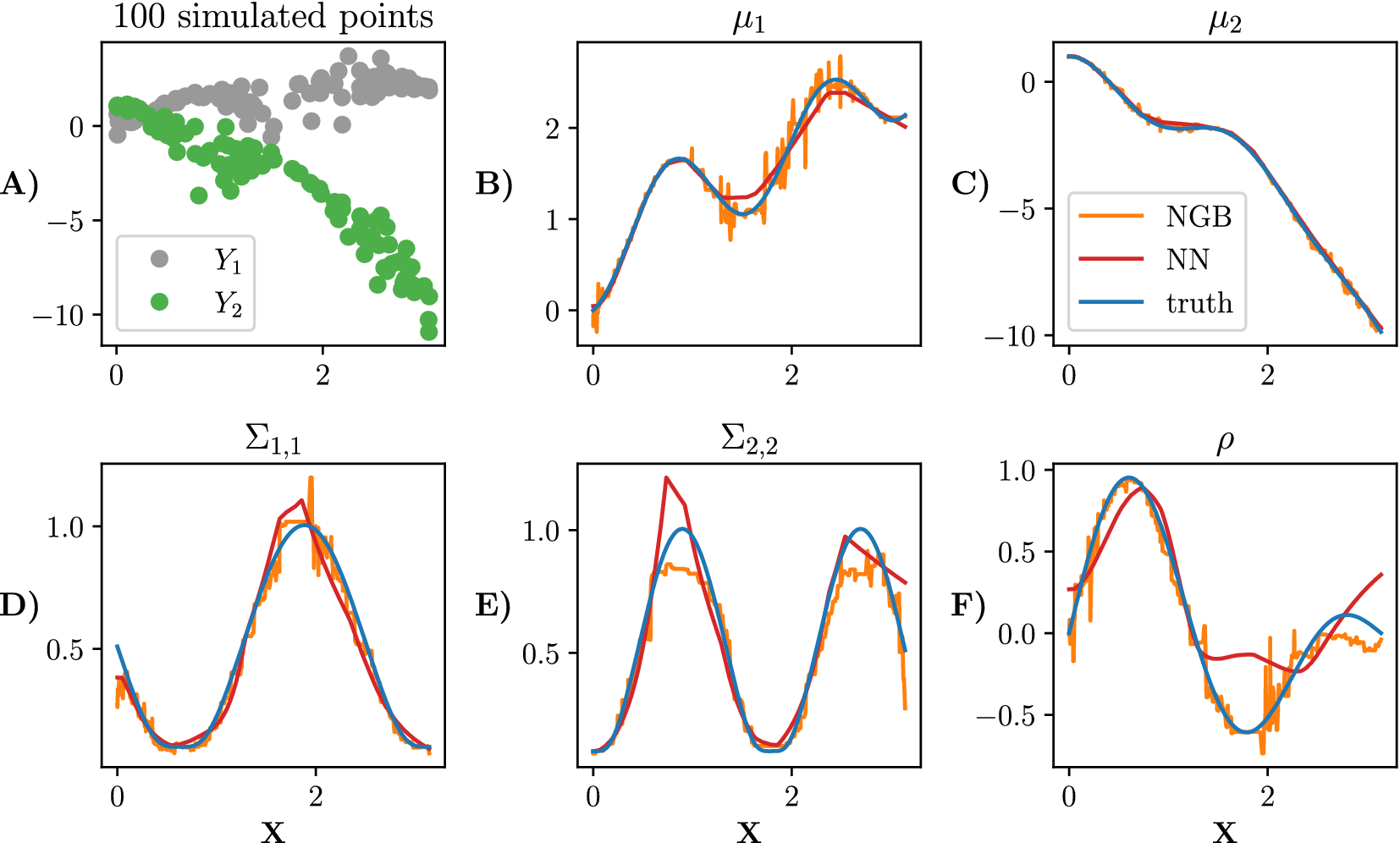
Simulated data alongside the true parameters are shown in Figure 1.
Simulated data from equation (5). A sample of 100 points is shown in panel (a). We plot each parameter in plots (b) to (f). The true parameters of the distribution are shown in blue, the NGBoost fit is shown in orange, and the neural network fit with one hidden layer (100 neurons in the hidden layer) is shown in red. Both model fits are trained on
![]() training points.
training points.
We compare multiple methods, all of which predict a multivariate Gaussian. For all boosting models, we use scikit-learn decision trees (Pedregosa et al., Reference Pedregosa, Varoquaux, Gramfort, Michel, Thirion, Grisel, Blondel, Prettenhofer, Weiss, Dubourg, Vanderplas, Passos, Cournapeau, Brucher, Perrot and Duchesnay2011) as the base learner. Specifically, we consider five different comparison methods:
-
• NGB: The method proposed in this paper: NGBoost to fit a multivariate Gaussian distribution.
-
• Indep NGB: Independent NGBoost where a univariate Gaussian model is fitted for the two dimensions separately, that is,
 . Early stopping allows the number of trees used to predict each dimension to differ.
 -
• skGB: Scikit-learn’s (Pedregosa et al., Reference Pedregosa, Varoquaux, Gramfort, Michel, Thirion, Grisel, Blondel, Prettenhofer, Weiss, Dubourg, Vanderplas, Passos, Cournapeau, Brucher, Perrot and Duchesnay2011) implementation of gradient boosting (skGB) is used as a point prediction approach. To turn the skGB predictions into a multivariate Gaussian, we estimate a constant diagonal covariance matrix based on the residuals of the training data. For metric computation, we assume that each
follows a multivariate Gaussian with mean from a model fit for each dimension, and constant covariance matrix. Similar to Indep NGB, we allow a different number of trees for each dimension. This is the only model which does not have a covariance matrix varying over
. -
• GB: A multi-parameter gradient boosting algorithm, where the only change from NGB is that the gradients are not multiplied by
. -
• NN: The neural network approach from Williams (Reference Williams1996) discussed in Section 2.2. We fit the model using tensorflow (Abadi et al., Reference Abadi, Barham, Chen, Chen, Davis, Dean, Devin, Ghemawat, Irving, Isard, Kudlur, Levenberg, Monga, Moore, Murray, Steiner, Tucker, Vasudevan, Warden, Wicke, Yu and Zheng2016). More details about the model and the grid search carried out on the network structure are explained in the Supplementary Material.
To prevent overfitting, we employ early stopping for all methods on the held-out validation set, where we use a patience of 50 for all methods. For all boosting approaches, we use the estimators up to the best iteration that was found, and for neural networks we restore the weights back to the best epoch. The base learner for all boosting approaches are run using the default parameters specified in each package. For each N considered in the experiment, the neural network structure with the best log-likelihood metric averaged over all replications is chosen from the grid search. A learning rate of 0.01 is used for all methods, for NN, we use the Adam optimizer (Kingma and Ba, Reference Kingma, Ba, Bengio and LeCun2015).
We train the models used in the experiment with
![]() with 50 replications for each value of N. For each simulation, N values were simulated as the training dataset. In addition to the N values, 300 values were simulated as the validation set for early stopping, and another 1000 values were used as the test set. We then use the Kullback–Leibler (KL) divergence from the true distribution at the test-set locations as the main comparison metric, however, we report extended results with extra metrics in the Supplementary Material.
with 50 replications for each value of N. For each simulation, N values were simulated as the training dataset. In addition to the N values, 300 values were simulated as the validation set for early stopping, and another 1000 values were used as the test set. We then use the Kullback–Leibler (KL) divergence from the true distribution at the test-set locations as the main comparison metric, however, we report extended results with extra metrics in the Supplementary Material.
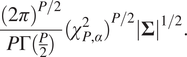
The per-model results on the test data points are shown in Table 1. The average KL divergence from the predicted distribution to true distribution is used as a metric. The results show that the NGB method is best for all N despite not being tuned in any way besides early stopping. The KL divergence converges quickly to 0 as N grows, showing that NGB gets better at learning the distribution as N increases. NN performs worse than NGB with higher KL divergence for all values of N. The KL divergence for Indep NGB seems to converge to a nonzero quantity as N increases, likely because the true distribution in equation (5) cannot be captured by a multivariate normal with a diagonal covariance matrix. skGB has large KL divergences which get worse as N increases, likely because of the homogeneous variance fit. We note that GB performs significantly worse than NGB showing that the natural gradient is necessary to fit the multivariate Gaussian effectively with boosting. Further metrics can be seen in the Supplementary Material, in particular, they show that GB fits the mean
![]() very poorly, which is then compensated for by a large covariance estimate, explaining the large KL divergence.
very poorly, which is then compensated for by a large covariance estimate, explaining the large KL divergence.
Average KL divergence in the test set (to three decimal places) from the predicted distribution to the true distribution as the number of training data points N varies.
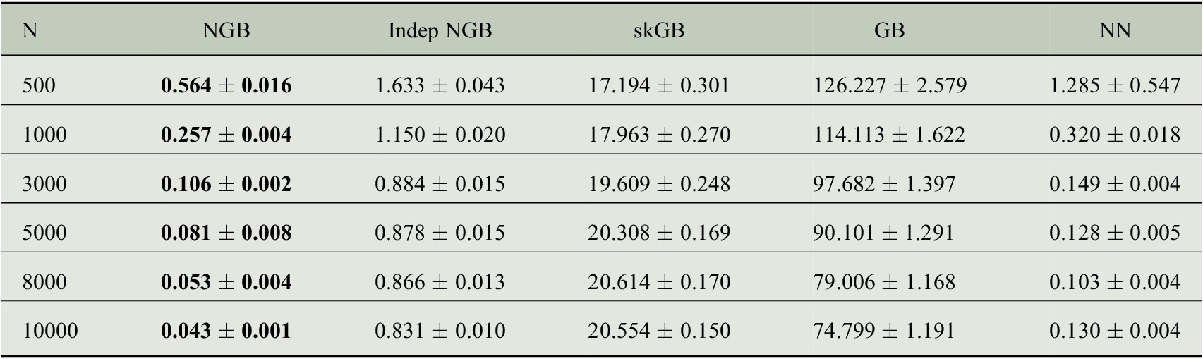
Note. Standard error estimated from 50 replications reported after
![]() to three decimal places. Lower values are better, the result with the lowest mean is bolded in each row. An extended table showing additional metrics is shown in the Supplementary Material.
to three decimal places. Lower values are better, the result with the lowest mean is bolded in each row. An extended table showing additional metrics is shown in the Supplementary Material.
The modification we made from the simulation in Williams (Reference Williams1996) is that we added
![]() and
and
![]() terms to
terms to
![]() and
and
![]() , respectively, in equation (5). This modification is to highlight where our method excels and shows how robust the natural gradient methods are. We also ran the original simulation without the modification, where the results are given in the Supplementary Material. As a summary, we note the two major differences: (a) The gaps between NGB, GB, and NN are much smaller without the modification, implying that the addition of
, respectively, in equation (5). This modification is to highlight where our method excels and shows how robust the natural gradient methods are. We also ran the original simulation without the modification, where the results are given in the Supplementary Material. As a summary, we note the two major differences: (a) The gaps between NGB, GB, and NN are much smaller without the modification, implying that the addition of
![]() and
and
![]() terms causes the GB method to perform much worse. (b) Without the modification, the NN method does best for
terms causes the GB method to perform much worse. (b) Without the modification, the NN method does best for
![]() , whereas NGB continues to preform best for
, whereas NGB continues to preform best for
![]() .
.
In simulation results in the Supplementary Material, where
![]() and
and
![]() are not included in equation (5), GB achieves the lowest RMSE. Thus suggests that GB only has difficulty learning the mean when adaptation of
are not included in equation (5), GB achieves the lowest RMSE. Thus suggests that GB only has difficulty learning the mean when adaptation of
![]() and
and
![]() is included which explains the poor result from GB in Table 1. As noted the only difference between NGB and GB is that we do not pre-multiply by the inverse Fisher information, hence, we can attribute this difference in performance to the natural gradient.
is included which explains the poor result from GB in Table 1. As noted the only difference between NGB and GB is that we do not pre-multiply by the inverse Fisher information, hence, we can attribute this difference in performance to the natural gradient.
5. Ocean Drifters Application
The motivating application of this paper is to predict two-dimensional oceanographic velocities from satellite data on a large spatial scale. Typically, velocity prediction is done through physics-inspired parametric models fitted with least-squares or similar metrics, treating the directional errors as independent (Mulet et al., Reference Mulet, Rio, Etienne, Artana, Cancet, Dibarboure, Feng, Husson, Picot, Provost and Strub2021). In this section, we shall instead focus on a data-driven approach utilizing a number of observational datasets.
5.1. Data
Here, we introduce the datasets used which shall define
![]() ,
,
![]() . The data for all sources are available from 1992 to 2019 inclusive. All raw data sources are publicly available online, however, we also provide the processed ready to use dataset for future comparisons at https://doi.org/10.5281/zenodo.5644972.
. The data for all sources are available from 1992 to 2019 inclusive. All raw data sources are publicly available online, however, we also provide the processed ready to use dataset for future comparisons at https://doi.org/10.5281/zenodo.5644972.
For the model output
![]() , we seek to predict two-dimensional oceanic near-surface velocities as functions of global remotely sensed climate data. The dataset used to train, validate and test our model comes from the Global Drifter Program, which contains transmitted locations of freely drifting buoys (known as drifters) as they drift in the ocean and measure near-surface ocean flow.
, we seek to predict two-dimensional oceanic near-surface velocities as functions of global remotely sensed climate data. The dataset used to train, validate and test our model comes from the Global Drifter Program, which contains transmitted locations of freely drifting buoys (known as drifters) as they drift in the ocean and measure near-surface ocean flow.
The quality controlled 6-hourly product is used (Lumpkin and Centurioni, Reference Lumpkin and Centurioni2019) to construct the velocity data points which will be the outputs we aim to predict. We drop drifter observations which have a high location noise estimate, and we apply a low-pass filter to the velocities at 1.5 times the inertial period (a timescale determined by the Coriolis effect), this preprocessing follows previous similar works (Laurindo et al., Reference Laurindo, Mariano and Lumpkin2017). We only use data from drifters which still have a holey sock drogue, which is a drogue attached by a tether and is designed such that when attached the drifter will follow ocean near-surface flow. We use the inferred two-dimensional velocities of these drifters as our outputs
![]() .
.
The longitude–latitude locations of these observations and the time of year (percentage of 365) are used as three of the nine features in
![]() to account for spatial and seasonal effects. For the remaining six features in
to account for spatial and seasonal effects. For the remaining six features in
![]() , we use two-dimensional longitude–latitude measurements of geostrophic velocity (
, we use two-dimensional longitude–latitude measurements of geostrophic velocity (
![]() ), surface wind stress (
), surface wind stress (
![]() ), and wind speed (
), and wind speed (
![]() ). These variables are used as they jointly capture geophysical effects known as geostrophic currents, Ekman currents, and wind forcing, which are known to drive oceanic near-surface velocities. We obtain geostrophic velocity and wind measurements from data products Thematic Assembly Centers (2020a) and Thematic Assembly Centers (2020b) respectively, where the data products are interpolated to the longitude–latitude locations of interest. We further preprocess the data as explained in Appendix A.
). These variables are used as they jointly capture geophysical effects known as geostrophic currents, Ekman currents, and wind forcing, which are known to drive oceanic near-surface velocities. We obtain geostrophic velocity and wind measurements from data products Thematic Assembly Centers (2020a) and Thematic Assembly Centers (2020b) respectively, where the data products are interpolated to the longitude–latitude locations of interest. We further preprocess the data as explained in Appendix A.
To allow us to run multiple model fits, we subset the data to only include data points which are spatially located in the North Atlantic Ocean as defined by IHO marine regions (Flanders Marine Institute, 2018) and between 83°W and 40°W longitude. We also down-sample the data to daily intervals. Ultimately, this results in 414697 observations which we will use to compare the probabilistic regression models.
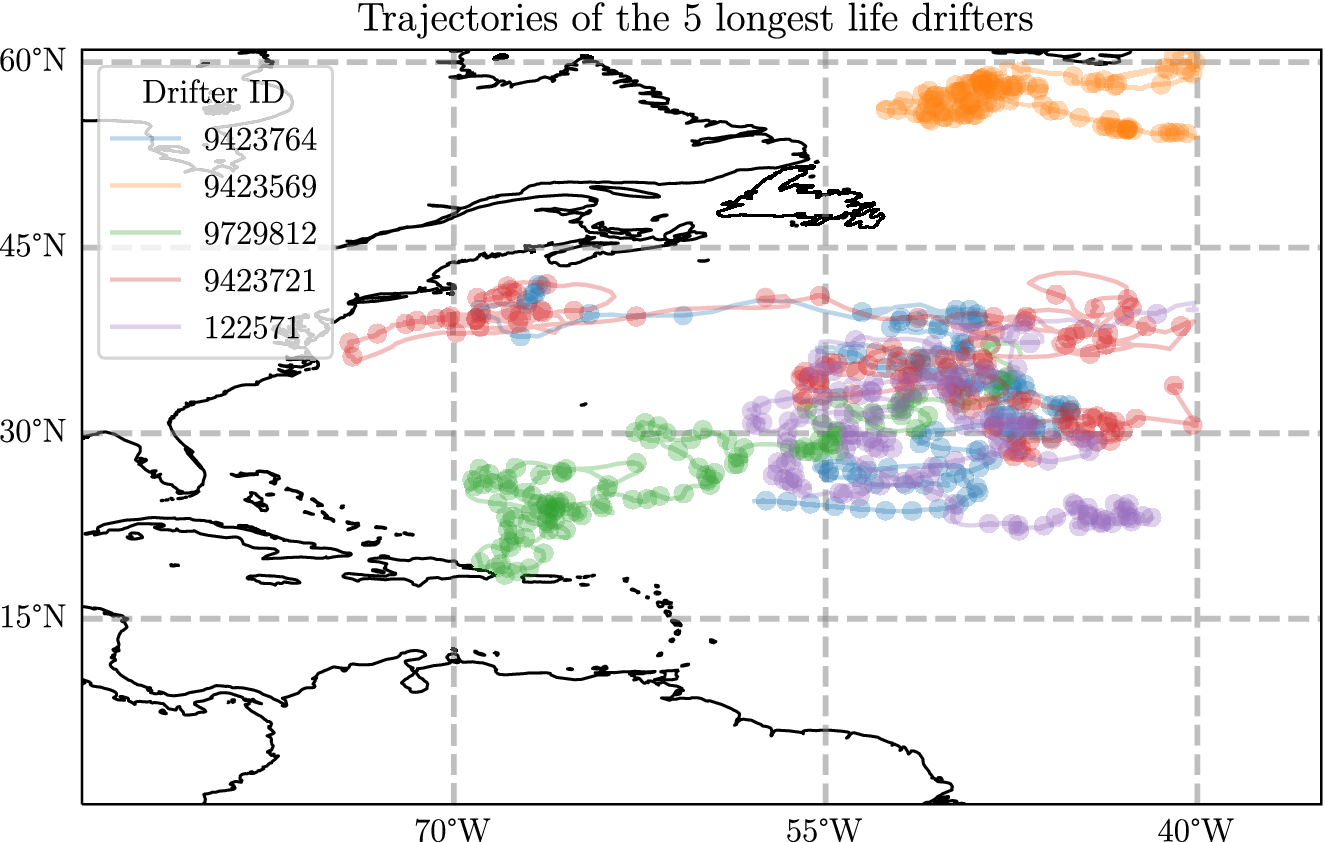
To give an insight into this dataset in Figure 2, we show the five longest trajectories used in this analysis. In particular, one of the features to notice is that there are areas where the sampled points are quite close together. For example, even though the northernmost trajectory is almost as long as the rest it seems to travel a much smaller distance overall. The drifters that start in the west, however, travel very long distances overall. This motivates the use of probabilistic regression algorithms, as the velocity measurement will have very different magnitudes depending on where in space they are and other factors. Additionally, we may suspect that the prediction error will be larger when the underlying velocity is larger.
A plot showing the five longest trajectories in the dataset described in detail in Appendix A, where each drifter has a lifetime of between 1100 and 1378 days. A point is plotted every 10 days.
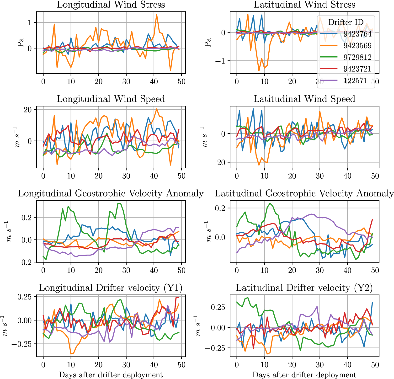
In Figure 3, we display a subset of the predictor variables
![]() for the first 50 days of the same drifters shown in Figure 2. In general, the geostrophic variables show strongest correlation to the
for the first 50 days of the same drifters shown in Figure 2. In general, the geostrophic variables show strongest correlation to the
![]() data for the respective dimensions. We do not show three of the nine dimensions in
data for the respective dimensions. We do not show three of the nine dimensions in
![]() in this plot: longitude, latitude or days since January 1st. These are not shown in the plot as, in general, we do not expect these relationships to be linear, hence the need for more complicated models.
in this plot: longitude, latitude or days since January 1st. These are not shown in the plot as, in general, we do not expect these relationships to be linear, hence the need for more complicated models.
The values of the prediction feature
![]() for the sample of drifters shown in Figure 2. We only show the first 50 days to allow the reader to see the more granular patterns.
for the sample of drifters shown in Figure 2. We only show the first 50 days to allow the reader to see the more granular patterns.
As a note, we do not exploit the grouped time-series structure of the drifter data in this work. When fitting the models, we ignore the drifter identification (ID) and just concatenate all data together. We learn a purely spatiotemporal model. If the goal was to forecast the location or velocity of the drifter at time
![]() and we knew the history up to time t then exploiting information such as the velocity at time t would likely be an informative feature to use.
and we knew the history up to time t then exploiting information such as the velocity at time t would likely be an informative feature to use.
5.2. Metrics
Unlike in the simulation, here, there is no ground truth, hence, we cannot use KL divergence as in Section 4 because the true distributions of these data are unknown. We shall instead use held-out data validation. We use a series of performance metrics that diagnose model fit which we introduce now.
Negative log-likelihood (NLL): All methods are effectively minimizing the negative log-likelihood; therefore, we use the negative log-likelihood as one of our metrics:

RMSE: To compare the point prediction performance of the models, we also report an average root mean squared error (RMSE):

Region coverage and area: As this paper focuses on a measure of probabilistic prediction, we also report metrics related to the prediction region. The prediction region is the multivariate generalization of the one-dimensional prediction interval. The two related summaries of interest are: (a) the percentage of
covered by the
prediction region, and (b) the area of the prediction region.
A
![]() prediction region can be defined for the multivariate Gaussian distribution as the set of values
prediction region can be defined for the multivariate Gaussian distribution as the set of values
![]() which satisfy the following inequality:
which satisfy the following inequality:
where
![]() is the quantile function of the
is the quantile function of the
![]() distribution with
distribution with
![]() degrees of freedom evaluated at
degrees of freedom evaluated at
![]() . This prediction region forms a hyper-ellipse which has an area given by
. This prediction region forms a hyper-ellipse which has an area given by
To use this as a metric, we report coverage as the percentage of data points which satisfy equation (6), and we report the average area of the prediction region over all points in the dataset. These metrics will be used in Table 2 in the next section.
Average test set metrics defined in Section 5.2.
Note. Standard error estimated from 10 replications reported after
![]() . PR stands for prediction region. Coverage has been shortened to cov. All numbers rounded to two decimal places, aside from the 90% PR area row which is rounded to the nearest integer. Lower values are better for NLL and RMSE, best value is bolded in both rows.
. PR stands for prediction region. Coverage has been shortened to cov. All numbers rounded to two decimal places, aside from the 90% PR area row which is rounded to the nearest integer. Lower values are better for NLL and RMSE, best value is bolded in both rows.
5.3. Results
We compare the same five models considered in Section 4. To compare the models, we randomly split the dataset, keeping each individual drifter record within the same set. We put 10% of records into the test set, 9% of records into the validation set, and 81% into the training set. The model is fitted to the training set with access to the validation set for early stopping, and then the metrics from Section 5.2 are evaluated on the test set. This procedure is repeated 10 times. The aggregated metrics are shown in Table 2.
For this example, we also use a grid search for all the boosting approaches, in addition to the neural network approach. The reason we do this is because we found that with the default parameters used in Section 4 early stopping did not occur, suggesting that the base learner may not be flexible enough. For each boosting method, a grid search is carried out on the number of leaves and minimum data in leaves, as outlined in the Supplementary Material. The best hyperparameters from the grid search for each method are selected by evaluating the test set negative log-likelihood.
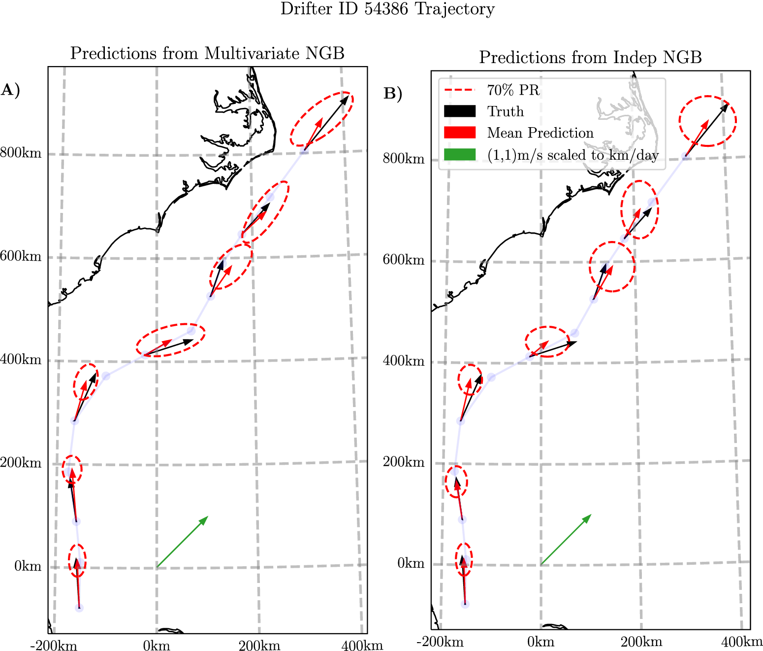
The aggregated results of the model fits are shown in Table 2. NGB and Indep NGB perform very similarly in terms of NLL, RMSE, and 90% PR coverage in this example. However, NGB provides a smaller 90% PR area, which is expected as correlation will reduce
![]() in equation (7). To further highlight the differences, we show the spatial differences in negative log-likelihood between these two methods in Figure 4b. In Figure 4c,d, we show the averaged held out spatial predictions for
in equation (7). To further highlight the differences, we show the spatial differences in negative log-likelihood between these two methods in Figure 4b. In Figure 4c,d, we show the averaged held out spatial predictions for
![]() and
and
![]() from the NGB model. The results shown in Figure 4b,c suggest that using a combination of NGB and Indep NGB may be suitable for this application. For example, we could use the NGB model in geographic areas with high anticipated correlation; and otherwise we could use Indep NGB.
from the NGB model. The results shown in Figure 4b,c suggest that using a combination of NGB and Indep NGB may be suitable for this application. For example, we could use the NGB model in geographic areas with high anticipated correlation; and otherwise we could use Indep NGB.
Summaries of test set results within
![]() latitude–longitude bins for the North Atlantic Ocean application. Panel (a) shows the spatial distribution of where the data are sampled. Panel (b) shows the difference between the negative log-likelihood spatially between NGB and Indep NGB; negative values (blue) implying NGB is better than Indep NGB (with vice versa in red). Panel (c) shows the average prediction of
latitude–longitude bins for the North Atlantic Ocean application. Panel (a) shows the spatial distribution of where the data are sampled. Panel (b) shows the difference between the negative log-likelihood spatially between NGB and Indep NGB; negative values (blue) implying NGB is better than Indep NGB (with vice versa in red). Panel (c) shows the average prediction of
![]() , where
, where
![]() is extracted from the predicted covariance matrix in the held out set from NGB. Panel (d) shows the mean currents estimated by NGB. All major ocean features are captured by the model (Lumpkin and Johnson, Reference Lumpkin and Johnson2013).
is extracted from the predicted covariance matrix in the held out set from NGB. Panel (d) shows the mean currents estimated by NGB. All major ocean features are captured by the model (Lumpkin and Johnson, Reference Lumpkin and Johnson2013).

In Table 2, we see that the NN and GB approaches generally perform poorly. Both methods have a large root mean squared error, which is compensated for by a larger prediction region on average, as can be concluded from the large average PR area. This behavior agrees with the univariate example given in Figure 4 of the NGBoost paper (Duan et al., Reference Duan, Anand, Ding, Thai, Basu, Ng, Schuler, Daumé and Singh2020), and the behavior of GB in the simulation of Section 4.
One of the novelties of this work is that we model the dependence between the two output dimensions. Any region where
![]() is close to 0 in figure 4c likely means that this additional modeling of the dependence will not make a significant difference in the predictions. In contrast, any region where the absolute value of
is close to 0 in figure 4c likely means that this additional modeling of the dependence will not make a significant difference in the predictions. In contrast, any region where the absolute value of
![]() is large implies that NGB predictions will be significantly different from Indep NGB. In particular, NGB predicts large values of
is large implies that NGB predictions will be significantly different from Indep NGB. In particular, NGB predicts large values of
![]() around the South Equatorial and Gulf Stream currents.
around the South Equatorial and Gulf Stream currents.
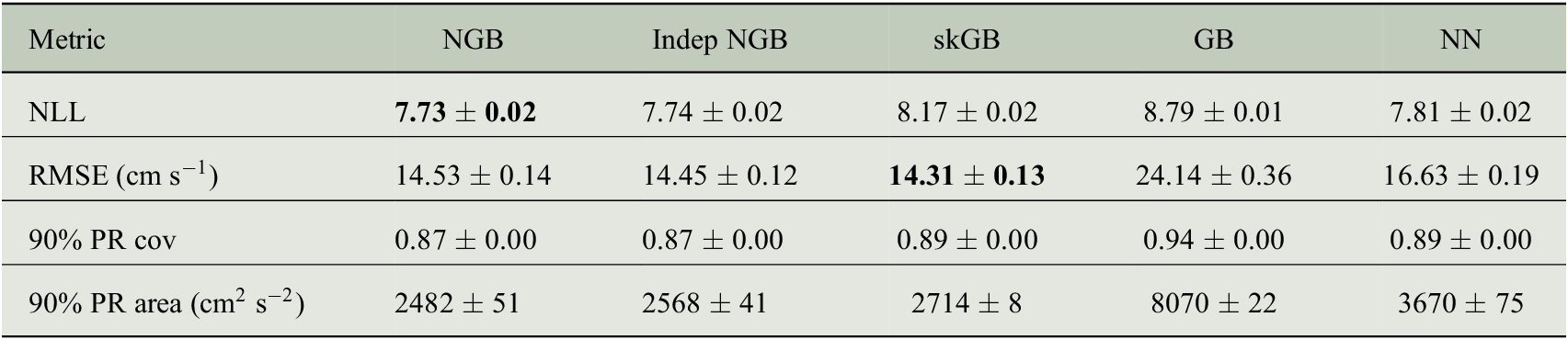
In Figure 5, we show a sample trajectory on the Gulf Stream alongside the predicted means and the 70% prediction region from both Indep NGB and NGB. In Figure 5a, the main factor to note is that the elliptical prediction regions of NGB take various orientations on the trajectory, most of which have the major axis aligned with the flow. In contrast, the predictions from Indep NGB in Figure 5b show the ellipses’ major axes are always either aligned with the longitudinal or latitudinal axis, as must be the case. This difference is particularly evident in the latter half of the shown trajectory, when traveling north–east, where Indep NGB’s predictions show a larger minor axis in the ellipses in comparison to NGB predictions. This is probably the key reason why NGB performs better on average around the Gulf Stream, as seen in Figure 4b.
Plots showing the predictions from both NGB (a) and Indep NGB (b) for the first 12 days of drifter ID 54386 starting from September 23, 2005. The velocity predictions are plotted every 2 days for visualization purposes. The velocity measurements are translated to where the drifter would end up after 1 day if it continued at the constant predicted velocity for visualization purposes. The model used for the prediction did not see this trajectory when trained. The faded blue line shows the trajectory of the drifter with a plotted point every day. The 70% prediction region is the boundary from equation (6). The 70% level is just chosen for visualization purposed to prevent the ellipses from overlapping in the plot. Conversion to easting-northing computed using a transverse Mercator projection centered at
![]() latitude and
latitude and
![]() longitude.
longitude.
5.4. Investigation into multivariate NGBoost against independent NGBoost
As is clear in the metrics shown in Table 2, the NGB method we have developed is only marginally better than the Indep NGB in terms of negative log-likelihood. This is despite the fact that the model that predicts a multivariate Gaussian seems to be better suited to the problem. The distribution where each dimension is just a univariate Gaussian is a special case of the multivariate Gaussian.
One potential reason may be related to overfitting. In the learning, we allow early stopping to alter the number of boosting rounds. In NGB, the way model fitting works is that we require every parameter to be predicted by
![]() base learners, whereas with Indep NGB, we allow the two models (one for longitudinal and one for latitudinal) to have different numbers of base learners
base learners, whereas with Indep NGB, we allow the two models (one for longitudinal and one for latitudinal) to have different numbers of base learners
![]() The longitudinal model generally chose to use more decision trees than the latitudinal direction. Thus, the early stopping used by Indep NGB has extra power in comparison to NGB. Further developments in the learning algorithm or fine-tuning of parameters of the base learner may correct this.
The longitudinal model generally chose to use more decision trees than the latitudinal direction. Thus, the early stopping used by Indep NGB has extra power in comparison to NGB. Further developments in the learning algorithm or fine-tuning of parameters of the base learner may correct this.
Another potential reason may be due to sampling, an argument which will be examined here. We find that NGB does better in areas with strong non-axes aligned currents like the Gulf Stream. For example, if we filter the test data used to calculate the entries in Table 2 to an area which is primarily made up of the Gulf Stream, we find that the improvement is more noticeable; consider the box with corners
![]() which is a section largely made up of the Gulf Stream. This area is shown in Figure 6. The average likelihood is 9.46 for NGB and 9.52 for Indep NGB on this subset of the data. That is a larger difference in likelihood than what we observed in the unfiltered dataset in Table 2. We show this difference in NLL across this smaller region in Figure 6b; we note that in some areas, NGB is doing much better, particularly in boxes with stronger currents, which can be identified using Figure 6d).
which is a section largely made up of the Gulf Stream. This area is shown in Figure 6. The average likelihood is 9.46 for NGB and 9.52 for Indep NGB on this subset of the data. That is a larger difference in likelihood than what we observed in the unfiltered dataset in Table 2. We show this difference in NLL across this smaller region in Figure 6b; we note that in some areas, NGB is doing much better, particularly in boxes with stronger currents, which can be identified using Figure 6d).
The same metrics as shown in Figure 4, just zoomed in on a smaller section which is analyzed in Section 5.4. The plot has a finer granularity than Figure 4, the resolution here is a
![]() bin granularity. The definition of the plotted metrics in panels A-D) can be found in the caption of Figure 4.
bin granularity. The definition of the plotted metrics in panels A-D) can be found in the caption of Figure 4.
Another observation that can be seen is where NGBoost is doing worse than Indep NGB on average. In particular, the spatial boxes near the coast around
![]() in Figure 6b, where Indep NGB is doing better (positive difference). By looking at the same boxes in Figure 6a,c, we can observe that these areas have few data points and returns a high predicted average correlation from the NGB method. A potential reason for Indep NGB doing better in this specific region is that Indep NGB is benefiting from the independence assumption. There is not enough data for NGB to learn that correlation is not strong in this specific region so NGB extrapolates information from the nearby regions. We can make a similar observation for the region around the bottom right corner of Figure 4b where Indep NGB is doing better in multiple boxes, and there are few data points, but NGB predicts a strong negative correlation.
in Figure 6b, where Indep NGB is doing better (positive difference). By looking at the same boxes in Figure 6a,c, we can observe that these areas have few data points and returns a high predicted average correlation from the NGB method. A potential reason for Indep NGB doing better in this specific region is that Indep NGB is benefiting from the independence assumption. There is not enough data for NGB to learn that correlation is not strong in this specific region so NGB extrapolates information from the nearby regions. We can make a similar observation for the region around the bottom right corner of Figure 4b where Indep NGB is doing better in multiple boxes, and there are few data points, but NGB predicts a strong negative correlation.
A final observation is that areas such as the Gulf Stream have very large velocities. The sampling to create this dataset is carried out temporally, where we sampled one point for every day. To examine the significance of this, we reuse the example shown in Figure 5; this trajectory follows the Gulf Stream and it travels the distance shown over 12 days; contributing only 12 points to the dataset even though it covers around 1073 km. On the other hand, consider drifter 122571 shown in Figure 2, to travel 1073 km this drifter took approximately 113 days, hence for the same distance, drifter 11257 contributes almost 10 times more to the evaluation used in Table 2. On average, over the trajectory of drifter 11257, Indep NGB achieved a lower NLL. In summary, due to the nature of the data sampling procedure used here, in the evaluation we give more weight to regions with lower velocities. From Figure 4b,d, we can infer that in lower velocity regions Indep NGB usually has a lower NLL. Hence, we are likely giving too much weight in the objective to drifters in areas with weaker currents; this likely explains the relatively small differences in Table 3.
Summary of data used in the application.
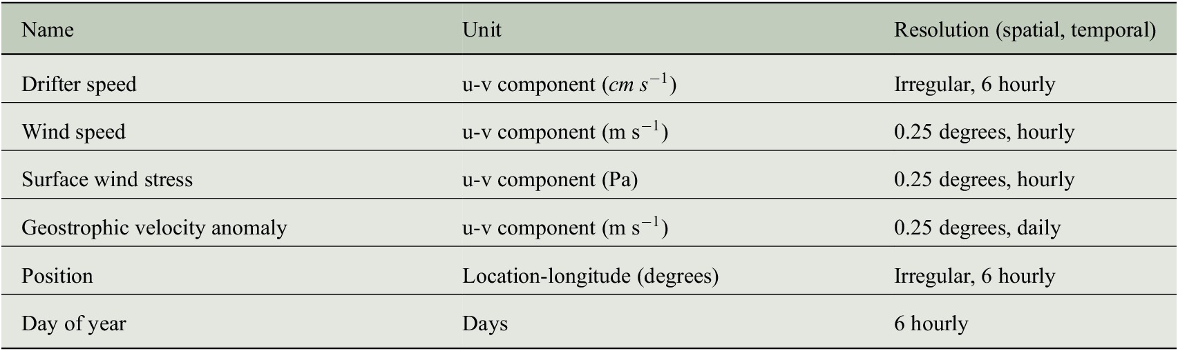
Note. Drifter speed is used to define the two-dimensional response
![]() . The rest of the variables listed defined the nine features used for
. The rest of the variables listed defined the nine features used for
![]() .
.
In summary, the conclusions from our study are that NGB shows improvements over Indep NGB in regions of strong currents where flow is correlated across dimensions, and in other regions of weak flow and correlation, the two methods perform similarly to each other. The exception to this rule is when data sparsity is present, for example, in the case around
![]() , where Indep NGB can sometimes outperform NGB. Overall, this suggests that NGB can be robustly applied across wide spatial regions, as well as specifically applied in regions where Indep NGB is expected to fail. If there is no correlation present, then Indep NGB will likely do better as the assumption of independence between output dimensions is then correct in a Gaussian setting.
, where Indep NGB can sometimes outperform NGB. Overall, this suggests that NGB can be robustly applied across wide spatial regions, as well as specifically applied in regions where Indep NGB is expected to fail. If there is no correlation present, then Indep NGB will likely do better as the assumption of independence between output dimensions is then correct in a Gaussian setting.
6. Conclusions
This paper has demonstrated the accuracy of our NGBoost method when focusing on bivariate outcomes with a multivariate Gaussian distribution. The derivations of the natural gradient and implementation in NGBoost are supplied for any dimensionality, but empirical proof of performance in higher dimensions is left to future work. Due to the quadratic relationship between P and the number of parameters used to parameterize the multivariate Gaussian, the complexity of the learning algorithm increases greatly with higher values of P. Investigating a reduced rank form of the covariance matrix may be of interest for higher P to reduce the number of parameters that must be learned.
Furthermore, the results shown here add to the collection of works that show large improvements in gradient-based learning when using natural gradients (Hoffman et al., Reference Hoffman, Blei, Wang and Paisley2013; Salimbeni et al., Reference Salimbeni, Eleftheriadis and Hensman2018; Duan et al., Reference Duan, Anand, Ding, Thai, Basu, Ng, Schuler, Daumé and Singh2020). In the simulation of Section 4, we showed how crucial the natural gradient is to fitting this model, as the “GB” approach essentially failed to learn. The same exact comparison is shown in the original NGBoost paper Duan et al. (Reference Duan, Anand, Ding, Thai, Basu, Ng, Schuler, Daumé and Singh2020) where GB performs significantly worse than the natural gradient approach. The simulations highlight the robustness of the natural gradient approaches in contrast to the ordinary gradient approaches, as we have shown how making a fairly simple adjustment (
![]() and
and
![]() to the mean terms) can yield a large difference in results.
to the mean terms) can yield a large difference in results.
The difference between NGB and Indep NGB was overall relatively small in our real-world application across the entire spatial domain studied, but NGB showed significant improvements around major currents such as the Gulf Stream where directional currents (that are not aligned with the
![]() axis) are most prominent. This improvement was corroborated in simulations where NGB performed relatively much better than Indep NGB overall. Generally, one should expect NGB to excel in cases with high correlation between the outcomes, whereas a method assuming independence should suffice when that assumption is warranted. Deep-learning approaches are warranted in cases where a neural network naturally handles the input space such as images, speech, or text.
axis) are most prominent. This improvement was corroborated in simulations where NGB performed relatively much better than Indep NGB overall. Generally, one should expect NGB to excel in cases with high correlation between the outcomes, whereas a method assuming independence should suffice when that assumption is warranted. Deep-learning approaches are warranted in cases where a neural network naturally handles the input space such as images, speech, or text.
The analysis in Section 5.4, raises interesting questions about how we should sample this dataset. What would the difference in model fit and results be if we chose to sample a point every 50 km rather than daily when forming our dataset? Such a change in data processing would end up giving more weight to regions where strong currents exist; and in calmer regions where velocities are very low, it could take days to obtain a single sample in the dataset. Alternatively, we could also attempt to combine NGB and Indep NGB using model averaging, and this is reserved for future work.
6.1. Final remarks
In this paper, we have proposed a technique for performing probabilistic regression on vector-valued outputs with NGBoost. We have implemented software in the ngboost Python package which makes joint probabilistic regression easy to do with just a few lines of code and little tuning. Our simulation shows multivariate NGBoost exceeds the performance of existing methods for multivariate probabilistic regression. We have demonstrated the value of modeling the covariance between dimensions on a novel oceanographic problem using Global Drifter Program and remotely sensed satellite data. Specifically, we found that multivariate NGBoost excels in predicting ocean velocities in spatial areas where data sparsity is not an issue and correlation between the output dimensions is present.
Author Contribution
Conceptualization: all authors; Data curation: M.O’M., R.L.; Data visualization: M.O’M.; Methodology: M.O’M., A.M.S., A.S.; Writing original draft: M.O’M., A.M.S. All authors approved the final submitted draft.
Competing Interest
The authors have no competing interests.
Data Availability Statement
Replication data for the oceanographic application from Section 4 can be found at https://doi.org/10.5281/zenodo.5644972. The code to reproduce the results and simulation can be found at https://github.com/MikeOMa/MV_Prediction (see release v0.2 for source code used throughout this paper), however, for practical use, one should use the ngboost Python package, a sample code snippet is shown in the Supplementary Material. The package is available from the Python package index and version 0.3.10 was used for this paper.
Ethics Statement
The research meets all ethical guidelines, including adherence to the legal requirements of the study country.
Funding Statement
This work was funded by the Engineering and Physical Sciences Research Council (Grant Nos. EP/L015692/1 to M.O’M. and EP/R01860X/1 to A.M.S.).
Supplementary Material
The supplementary material for this article can be found at https://doi.org/10.1017/eds.2023.4.
Acknowledgments
We would like to thank the anonymous reviewers for taking the time and effort necessary to review the manuscript. We received valuable comments and suggestions that helped us improve the quality of the manuscript. Additionally, we thank Ryan Wolbeck for their work maintaining NGBoost.
A. Appendix: Drifter Data Processing
For reproducibility, we give instructions on how the application dataset used in Section 4 is created. In its raw form, the drifter dataset is irregularly sampled in time; however, the product used here is processed to be supplied on a 6-hourly scale (Lumpkin and Centurioni, Reference Lumpkin and Centurioni2019) and includes location uncertainties. A high uncertainty would be caused by a large gap in the sampling of raw data or a large satellite positioning error. In our study, we dropped all drifter observations with a positional error greater than
![]() in longitude or latitudinal coordinates.
in longitude or latitudinal coordinates.
The six features that we used relate to wind stress, geostrophic velocity, and wind speed, and are all available on longitude–latitude grids, with spatial and temporal resolution specified in Table 3; we refer to these as gridded products. Before using these products to predict drifter observations, we spatially interpolatedFootnote
1 the gridded products to the drifter locations. To interpolate the gridded products, an inverse distance weighting interpolation was used. We only used the values at the
![]() corners that define the spatial box containing the longitude–latitude location of the drifter location of interest, where the following estimate is used:
corners that define the spatial box containing the longitude–latitude location of the drifter location of interest, where the following estimate is used:
where
![]() is the gridded value for the
is the gridded value for the
![]() corner (e.g., a
corner (e.g., a
![]() east–west geostrophic velocity at
east–west geostrophic velocity at
![]() longitude and
longitude and
![]() latitude),
latitude),
![]() is the inverse of the Haversine distanceFootnote
2 between the drifter’s longitude–latitude and the longitude–latitude location of the gridded value
is the inverse of the Haversine distanceFootnote
2 between the drifter’s longitude–latitude and the longitude–latitude location of the gridded value
![]() .
.
If two or more of the grid corners that are being interpolated from did not have a value recorded in the gridded product (e.g., if two corners were on a coastline in the case of wind stress and geostrophic velocity), we did not interpolate and treated that point as missing. If only one corner was missing, we use
![]() in equation (A.1), omitting the missing point.
in equation (A.1), omitting the missing point.
We low-pass filtered the drifter velocities, wind speed, and wind stress series to remove effects caused by inertial oscillations and tides; this process is similar to previous works (Laurindo et al., Reference Laurindo, Mariano and Lumpkin2017). A critical frequency of 1.5 times the inertial period (the inertial period is a function of latitude) was used. Due to missing or previously dropped data due to preprocessing steps, some time series have gaps in time larger than 6 hr. In such cases, we split that time series into individual continuous segments. We applied a fifth-order Butterworth low-pass filter to each continuous segment. If any of these segments were shorter than 18 observations (4.5 days), the whole segment was treated as missing from the dataset. The Butterworth filter was applied in a rolling fashion to account for the changing fashion of the inertial period, which defines the critical frequency.
The geostrophic data are available on a daily scale; therefore, we decimated all data to daily, only keeping observations at 00:00. No further preprocessing was performed on the geostrophic velocities (after interpolation) as inertial and tidal motions are not present in the geostrophic velocity product.
Finally, to remove poorly sampled regions from the dataset, we partitioned the domain into
![]() longitude–latitude non-overlapping grid boxes. We counted the number of daily observations contained in each box; if this count was less than 25, then the observations within that box were removed from the dataset. A link to download the processed data can be found at https://doi.org/10.5281/zenodo.5644972.
longitude–latitude non-overlapping grid boxes. We counted the number of daily observations contained in each box; if this count was less than 25, then the observations within that box were removed from the dataset. A link to download the processed data can be found at https://doi.org/10.5281/zenodo.5644972.
We only considered complete collections for
![]() ; If any of the data were recorded as missing in the process explained above, that daily observation was removed from the dataset. Before fitting the models, we scaled the training data
; If any of the data were recorded as missing in the process explained above, that daily observation was removed from the dataset. Before fitting the models, we scaled the training data
![]() to be in the range
to be in the range
![]() for all variables, this step was taken to make the neural network fitting more stable, this step will have no effect on the gradient boosting approaches.
for all variables, this step was taken to make the neural network fitting more stable, this step will have no effect on the gradient boosting approaches.
B. Appendix: Multivariate Normal Natural Gradient Derivations
To fit the NGBoost model, we require three elements, the log-likelihood, the derivative of the log-likelihood, and the Fisher information matrix. We use the parameterization for the multivariate Gaussian given in Section 2.2.
We shall derive results for the general case where
![]() is the dimension of the data
is the dimension of the data
![]() We use
We use
![]() to denote the value of the
to denote the value of the
![]() dimension of
dimension of
![]() in this section; a similar notation is used for
in this section; a similar notation is used for
![]() and
and
![]() . The probability density function can be written as
. The probability density function can be written as
As mentioned in Section 2, the optimization of
![]() is relatively straightforward, as it lives entirely on the unconstrained real line.
is relatively straightforward, as it lives entirely on the unconstrained real line.
![]() is an
is an
![]() positive definite matrix, which is a difficult constraint. Therefore, optimizing this directly is a challenge. Instead, if we consider the Cholesky decomposition of
positive definite matrix, which is a difficult constraint. Therefore, optimizing this directly is a challenge. Instead, if we consider the Cholesky decomposition of
![]() , where
, where
![]() is an upper triangular matrix, we only require that the diagonal be positive to ensure that
is an upper triangular matrix, we only require that the diagonal be positive to ensure that
![]() is positive definite. We choose to model the inverse of
is positive definite. We choose to model the inverse of
![]() as in Williams (Reference Williams1996).
as in Williams (Reference Williams1996).
Therefore, we form an unconstrained representation for
, where we denote
as the element in the
row and the
column as follows:

Hence, we can fit
by doing gradient-based optimization on
as all values live on the real line. As an example, for
, we can fit a multivariate Gaussian using unconstrained optimization through the parameter vector
.
As in Williams (Reference Williams1996), we simplify the parameters to

where, we have denoted
as the column vector of
. Throughout the following derivations, we will interchangeably use
without noting that these parameters have a mapping between them (e.g.,
).
Noting that
, the negative log-likelihood can be simplified as follows:

where
is a constant independent of
and
. For a shorter notation, we will write
.
The first derivatives are stated in Williams (Reference Williams1996) and we also state them here for reference:
The final element that we need for NGBoost to work is the
Fisher information matrix. This was not needed in Williams (Reference Williams1996), so we derive the Fisher information here. We start all calculations from the following definition:
Note that
![]() is a symmetric matrix, such that
is a symmetric matrix, such that
![]() . For convenience, we denote the entries of the matrix with the subscripts of the parameter symbols, for example,
. For convenience, we denote the entries of the matrix with the subscripts of the parameter symbols, for example,
![]() . We use the letters
. We use the letters
![]() to index the variables. The following two expectations are frequently used:
to index the variables. The following two expectations are frequently used:
![]() and
and
![]() .
.
The derivatives of
with respect to the other parameters are repeatedly used, so we give them here:

We start with the Fisher information for
, using the existing derivation of
in equation (A.3):

We therefore have that
Next, we consider the mean differentiated with respect to
again starting from equation (A.3):

As the expectation of both terms inside the sum is zero for every valid combination of
, we conclude that
Finally, the last elements that we require for the Fisher information matrix are the entries for
. First, we consider diagonals (
) w.r.t. all
with
. We start by using Equation (A.4) for
:

Taking the expectation, we get

Finally, we derive the Fisher information for the off diagonals with respect to the off diagonals
and
). We start from the expression for
in Equation (A.5):

Hence,
Equations (A.6)–(A.9) give the full specification of the Fisher information.


 Open access