


Impact Statement
Robust uncertainty quantification is important for the reliability of model predictions. Conformal prediction is a model-agnostic and distribution-free framework to obtain statistically valid prediction intervals, but remains underused in climate science. By applying and evaluating conformal prediction methods for microphysical process rates spanning several orders of magnitude, we demonstrate their potential for inexpensive uncertainty quantification in weather and climate modeling.
1. Introduction
In atmospheric prediction, purely deterministic methods increasingly reveal their limitations. For subgrid-scale parameterizations, grid-scale state variables may not uniquely determine the net effect of unresolved processes (Palmer, Reference Palmer2019; Christensen et al., Reference Christensen, Kouhen, Miller and Parthipan2024). This motivates probabilistic frameworks, stochastic parameterizations, and robust uncertainty quantification (Haynes et al., Reference Haynes, Lagerquist, McGraw, Musgrave and Ebert-Uphoff2023; Christensen et al., Reference Christensen, Kouhen, Miller and Parthipan2024; Schreck et al., Reference Schreck, Gagne, Becker, Chapman, Elmore, Fan, Gantos, Kim, Kimpara, Martin, Molina, Przybylo, Radford, Saavedra, Willson and Wirz2024; Mansfield and Christensen, Reference Mansfield and Christensen2025), often implemented through ensemble approaches (e.g., Gagne II et al., Reference Gagne, Christensen, Subramanian and Monahan2020; Behrens et al., Reference Behrens, Beucler, Iglesias-Suarez, Yu, Gentine, Pritchard, Schwabe and Eyring2025) that can be computationally costly.
As a computationally inexpensive alternative, conformal prediction (CP) (Gammerman et al., Reference Gammerman, Vovk and Vapnik1998; Angelopoulos and Bates, Reference Angelopoulos and Bates2022; Vovk et al., Reference Vovk, Gammerman and Shafer2022) provides distribution-free prediction intervals with finite-sample validity for any regression model, under the assumption that the data is exchangeable, which is weaker than the independent and identically distributed assumption commonly used in machine learning (ML). Yet, CP has seen limited use in weather and climate applications (e.g., Gopakumar et al. Reference Gopakumar, Gray, Oskarsson, Zanisi, Giles, Kusner, Pamela and Deisenroth2026; Mortier et al., Reference Mortier, Decancq, Sale, Javanmardi, Waegeman, Hüllermeier and Miralles2025), in part because spatio-temporal dependence in geophysical data can violate exchangeability. Extending conformal methods to such settings remains an active research area (e.g., Gibbs and Candès, Reference Gibbs and Candès2021; Xu and Xie, Reference Xu, Xie, Meila and Zhang2021; Sun, Reference Sun2022).
In numerical models, the spatial and temporal discretization separates resolved from unresolved scales. Subgrid-scale physical processes must therefore be represented through parameterizations, which are a major source of model uncertainty (Boucher et al., Reference Boucher, Randall, Artaxo, Bretherton, Feingold, Forster, Kerminen, Kondo, Liao, Lohmann, Rasch, Satheesh, Sherwood, Stevens and Zhang2014). Cloud microphysics describes phase transitions of condensed water in the atmosphere and interactions among liquid and frozen particles, water vapor, and aerosols. These processes control precipitation formation and intensity, impact storm evolution, and, through latent heating and cooling, influence cloud dynamics and large-scale cloud structure. Microphysical properties also affect radiative transfer and thus the Earth’s radiation budget (Gettelman et al., Reference Gettelman, Morrison, Thompson, Randall, Srinivasan, Nanjundiah and Mukhopadhyay2019; Morrison et al., Reference Morrison, Van Lier-Walqui, Fridlind, Grabowski, Harrington, Hoose, Korolev, Kumjian, Milbrandt, Pawlowska, Posselt, Prat, Reimel, Shima, Van Diedenhoven and Xue2020; Lamb et al., Reference Lamb, Singer, Loftus, Morrison, Powell, Ko, Buch, Hu, van Lier Walqui and Gentine2026). Accurate representation of cloud microphysics remains particularly challenging due to its inherent complexity and nonlinearity, as well as incomplete process-level understanding (Khain et al., Reference Khain, Beheng, Heymsfield, Korolev, Krichak, Levin, Pinsky, Phillips, Prabhakaran, Teller, van den Heever and Yano2015; Zelinka et al., Reference Zelinka, Myers, McCoy, Po-Chedley, Caldwell, Ceppi, Klein and Taylor2020). Improved understanding of cloud processes will help to reduce persistent uncertainties and advance the development of ML-based models (Lamb et al., Reference Lamb, Singer, Loftus, Morrison, Powell, Ko, Buch, Hu, van Lier Walqui and Gentine2026). Microphysical process rates (MPRs), computed internally to update the prognostic cloud variables, would provide detailed insights into cloud processes and support model development. Yet, storage constraints typically preclude saving MPR output from large-scale high-resolution simulations because MPRs comprise a two-digit number of three-dimensional variables. Moreover, offline recalculations of process rates are generally not accurate because of a temporal mismatch between the prognostic cloud variables in the model output and the MPRs computed during time stepping.
Here, we train ML models to emulate the computation of six MPRs from a two-moment bulk microphysics scheme (Seifert and Beheng, Reference Seifert and Beheng2006) and quantify predictive uncertainty with CP methods. Using ML emulators forced by atmospheric state variables from limited-area ICOsahedral Nonhydrostatic (ICON) simulations (Zängl et al., Reference Zängl, Reinert, Rípodas and Baldauf2015), we (i) apply split CP to calibrate prediction intervals for deterministic emulators, (ii) train quantile regression (QR) emulators and calibrate their intervals via conformalized quantile regression (CQR) (Romano et al., Reference Romano, Patterson and Candes2019), and (iii) benchmark interval calibration and sharpness across emulators and CP methods.
The structure is as follows. Section 2 reviews CP and CQR. Section 3 describes the MPRs, the ICON model output-based datasets, and the training and calibration procedure. Section 4 presents the results, and Section 5 concludes.
2. Theory: Conformal prediction
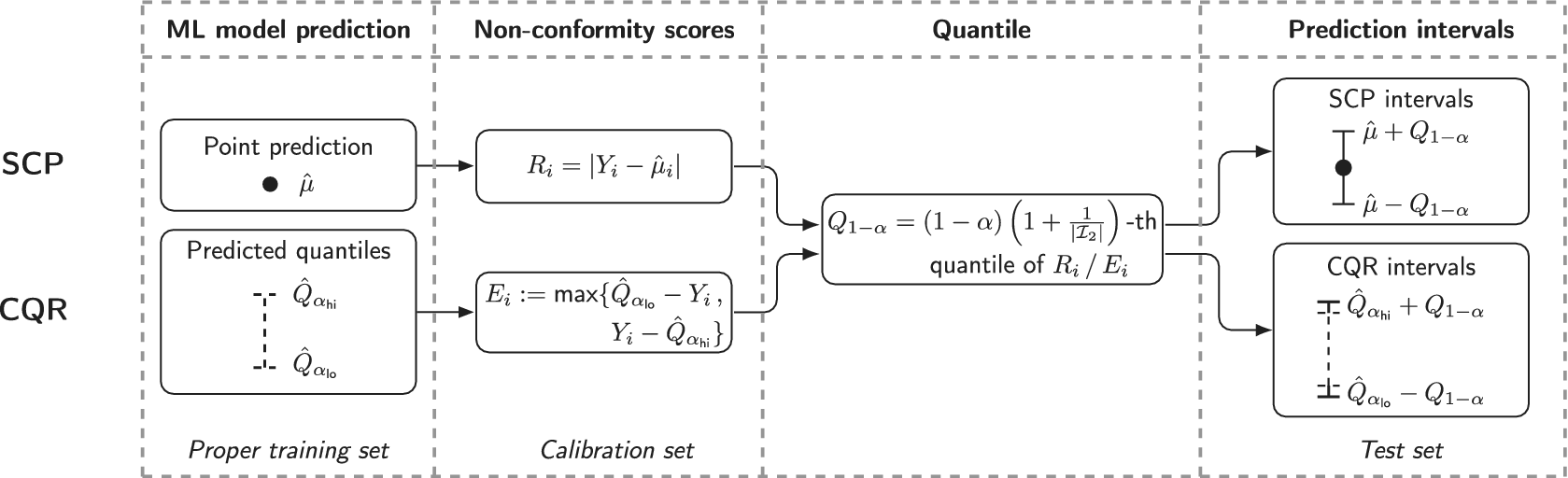
CP provides distribution-free prediction intervals for any regression or classification model, which contain the true value of the target with a pre-defined probability, requiring only data exchangeability (Vovk et al., Reference Vovk, Gammerman and Shafer2022). While originally formulated in a transductive setting (Gammerman et al., Reference Gammerman, Vovk and Vapnik1998), “full” CP is computationally expensive because it requires retraining the underlying model for each test point. We hence focus on inductive (“split”) CP, which is computationally efficient but requires splitting the data into a proper training set and a calibration set (Lei et al., Reference Lei, G’Sell, Rinaldo, Tibshirani and Wasserman2018). In split CP (Figure 1), a point-prediction model is trained on the proper training set, and nonconformity scores, which measure the prediction error, are computed on the calibration set. The
$ \left(1-\alpha \right) $
 -quantile of these scores sets the width of the prediction intervals. Here,
$ \alpha $
-quantile of these scores sets the width of the prediction intervals. Here,
$ \alpha $
 is a user-specified miscoverage rate, which quantifies the probability that the true value falls outside the prediction interval. This yields prediction intervals that, by construction, marginally contain the true target value with
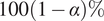
$ 100\left(1-\alpha \right)\% $
is a user-specified miscoverage rate, which quantifies the probability that the true value falls outside the prediction interval. This yields prediction intervals that, by construction, marginally contain the true target value with
$ 100\left(1-\alpha \right)\% $
 probability. Although this guarantee holds independently of model skill, data distribution, and nonconformity score function, interval informativeness mainly depends on the choice of score function (Angelopoulos and Bates, Reference Angelopoulos and Bates2022).
Conformal prediction framework: split conformal prediction (top row) and conformalized quantile regression (bottom row).
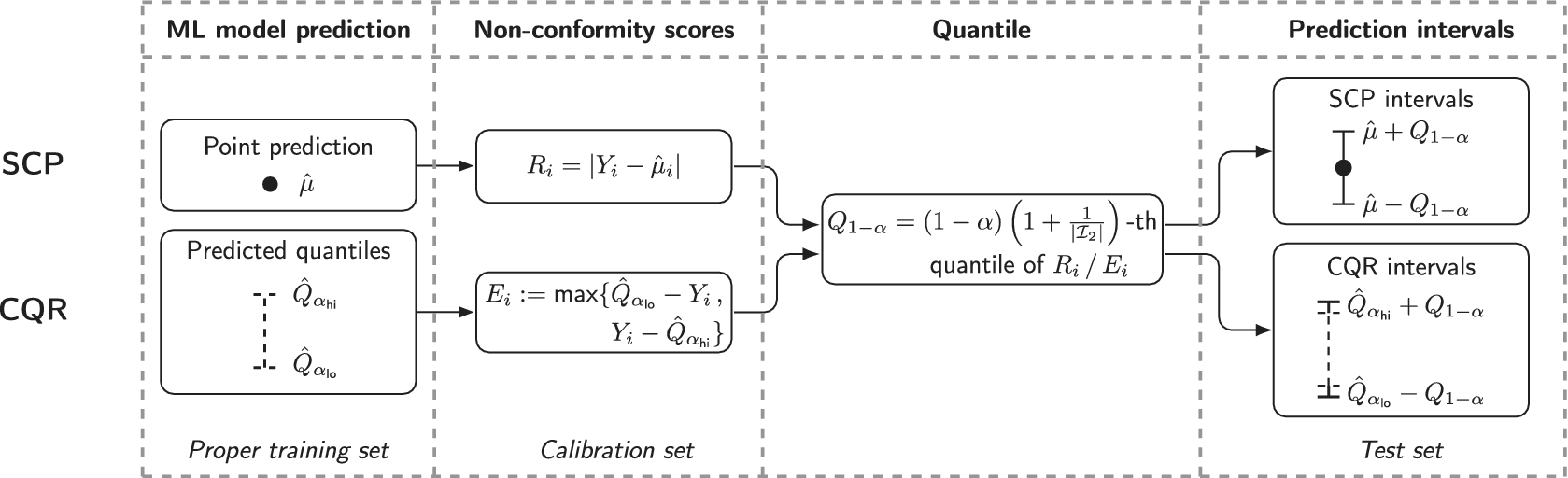
Figure 1. Long description
The diagram is organized into four vertical columns separated by dashed lines.
1. M L model prediction column (Proper training set):
- Top row (S C P): A box labeled Point prediction shows a black dot and mu-hat.
- Bottom row (C Q R): A box labeled Predicted quantiles shows a vertical dashed line between Q-hat sub alpha hi and Q-hat sub alpha lo.
2. Non-conformity scores column (Calibration set):
- Top row: A box contains the equation R sub i equals the absolute value of Y sub i minus mu-hat sub i.
- Bottom row: A box contains the equation E sub i is defined as the maximum of the set containing Q-hat sub alpha lo minus Y sub i and Y sub i minus Q-hat sub alpha hi.
3. Quantile column:
- A single central box receives arrows from both the S C P and C Q R non-conformity boxes. It contains the equation Q sub 1 minus alpha equals open parenthesis 1 minus alpha close parenthesis times open parenthesis 1 plus 1 over the absolute value of I sub 2 close parenthesis-th quantile of R sub i forward slash E sub i.
4. Prediction intervals column (Test set):
- Top row: A box labeled S C P intervals shows a vertical line with a central dot, bounded by mu-hat plus Q sub 1 minus alpha at the top and mu-hat minus Q sub 1 minus alpha at the bottom.
- Bottom row: A box labeled C Q R intervals shows a vertical dashed line bounded by Q-hat sub alpha hi plus Q sub 1 minus alpha at the top and Q-hat sub alpha lo minus Q sub 1 minus alpha at the bottom.
2.1. Split conformal prediction without retraining (SCP)
More formally, given
$ n $
 training samples
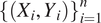
$ {\left\{\left({X}_i,{Y}_i\right)\right\}}_{i=1}^n $
training samples
$ {\left\{\left({X}_i,{Y}_i\right)\right\}}_{i=1}^n $
 , the main objective is to construct the prediction interval
$ \mathcal{C}\left({X}_{n+1}\right)\subseteq \mathrm{\mathbb{R}} $
, the main objective is to construct the prediction interval
$ \mathcal{C}\left({X}_{n+1}\right)\subseteq \mathrm{\mathbb{R}} $
 for a test point
$ {X}_{n+1} $
for a test point
$ {X}_{n+1} $
 . The interval
$ \mathcal{C} $
. The interval
$ \mathcal{C} $
 contains the unknown value
$ {Y}_{n+1} $
contains the unknown value
$ {Y}_{n+1} $
 with the miscoverage rate
$ \alpha \in \left(0,1\right) $
with the miscoverage rate
$ \alpha \in \left(0,1\right) $
 , satisfying the marginal coverage guarantee

for any joint distribution of the feature vectors
$ X\in {\mathrm{\mathbb{R}}}^p $
 of dimension
$ p\ge 1 $
of dimension
$ p\ge 1 $
 and labels
$ Y\in \mathrm{\mathbb{R}} $
and labels
$ Y\in \mathrm{\mathbb{R}} $
 and any sample size
$ n $
and any sample size
$ n $
 with the assumption that all samples
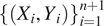
$ {\left\{\left({X}_i,{Y}_i\right)\right\}}_{i=1}^{n+1} $
with the assumption that all samples
$ {\left\{\left({X}_i,{Y}_i\right)\right\}}_{i=1}^{n+1} $
 are drawn exchangeably from the joint distribution.
The procedure for constructing the prediction intervals is straightforward. First, a regression model is trained on a proper training subset indexed by
$ {\mathcal{I}}_1\subset \left\{1,\dots, n\right\} $
 to predict
$ \hat{\mu}(x) $
to predict
$ \hat{\mu}(x) $
 . Then, a disjoint calibration subset indexed by
$ {\mathcal{I}}_2\subset \left\{1,\dots, n\right\} $
. Then, a disjoint calibration subset indexed by
$ {\mathcal{I}}_2\subset \left\{1,\dots, n\right\} $
 is used to compute the nonconformity scores

i.e., the residuals. Computing

with
$ \mid {\mathcal{I}}_2\mid $
 the cardinality of the calibration set, yields the prediction interval

which satisfies (2.1). Setting
$ \alpha =0.1 $
 corresponds to 90% prediction intervals.
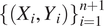
The coverage property (2.1) is marginal, i.e., averaged over all samples
$ {\left\{\left({X}_i,{Y}_i\right)\right\}}_{i=1}^{n+1} $
 (Romano et al., Reference Romano, Patterson and Candes2019; Feldman et al., Reference Feldman, Bates and Romano2021). The coverage guarantee holds for the distribution of the test point
$ {X}_{n+1} $
(Romano et al., Reference Romano, Patterson and Candes2019; Feldman et al., Reference Feldman, Bates and Romano2021). The coverage guarantee holds for the distribution of the test point
$ {X}_{n+1} $
 , but may not hold for the conditional distribution of
$ {Y}_{n+1} $
, but may not hold for the conditional distribution of
$ {Y}_{n+1} $
 given
$ {X}_{n+1} $
given
$ {X}_{n+1} $
 ,
,

which is referred to as conditional coverage and, in general, cannot be achieved (Lei and Wasserman, Reference Lei and Wasserman2012). As a result, the coverage probability can fall below
$ 100\left(1-\alpha \right)\% $
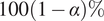 for subsets of the data, such as certain regimes or ranges of the target variable.
2.2. Conformalized quantile regression
While SCP allows for constructing marginally valid prediction intervals in a straightforward way at almost no additional computational cost, Eq. (2.4) reveals that the length of the prediction interval
$ \mathcal{C}\left({X}_{n+1}\right) $
 , is fixed to
$ 2{Q}_{1-\alpha}\left(R,{\mathcal{I}}_2\right) $
, is fixed to
$ 2{Q}_{1-\alpha}\left(R,{\mathcal{I}}_2\right) $
 , independent of the input
$ {X}_{n+1} $
, independent of the input
$ {X}_{n+1} $
 . SCP is based on the implicit assumption that the spread of the residuals is constant for all inputs
$ {X}_{n+1} $
. SCP is based on the implicit assumption that the spread of the residuals is constant for all inputs
$ {X}_{n+1} $
 , i.e., homoscedasticity, which is in practice often not the case. To address this issue, Romano et al. (Reference Romano, Patterson and Candes2019) proposed CQR. In CQR, a QR model is used to derive prediction intervals that can handle heteroscedasticity and thus are potentially more informative.
QR (Koenker and Bassett, Reference Koenker and Bassett1978) is a statistical method to estimate conditional quantiles of
$ {Y}_{n+1} $
 given
$ {X}_{n+1} $
given
$ {X}_{n+1} $
 , instead of the conditional mean. Here, a QR model is trained on the proper training dataset to predict the lower and upper quantile
$ {\hat{Q}}_{\alpha_{\mathrm{lo}}}(x) $
, instead of the conditional mean. Here, a QR model is trained on the proper training dataset to predict the lower and upper quantile
$ {\hat{Q}}_{\alpha_{\mathrm{lo}}}(x) $
 and
$ {\hat{Q}}_{\alpha_{\mathrm{hi}}}(x) $
and
$ {\hat{Q}}_{\alpha_{\mathrm{hi}}}(x) $
 , which constitute initial estimates of the lower and upper bound of the prediction interval,
$ \hat{\mathcal{C}}(x)=\left[{\hat{Q}}_{\alpha_{\mathrm{lo}}}(x),{\hat{Q}}_{\alpha_{\mathrm{hi}}}(x)\right] $
, which constitute initial estimates of the lower and upper bound of the prediction interval,
$ \hat{\mathcal{C}}(x)=\left[{\hat{Q}}_{\alpha_{\mathrm{lo}}}(x),{\hat{Q}}_{\alpha_{\mathrm{hi}}}(x)\right] $
 , with
$ {\alpha}_{\mathrm{lo}}=\alpha /2 $
, with
$ {\alpha}_{\mathrm{lo}}=\alpha /2 $
 and
$ {\alpha}_{\mathrm{hi}}=1-\alpha /2 $
and
$ {\alpha}_{\mathrm{hi}}=1-\alpha /2 $
 , e.g.,
$ \hat{\mathcal{C}}(x)=\left[{\hat{Q}}_{0.05},{\hat{Q}}_{0.95}\right] $
, e.g.,
$ \hat{\mathcal{C}}(x)=\left[{\hat{Q}}_{0.05},{\hat{Q}}_{0.95}\right] $
 . To quantify the error of this ad hoc prediction interval, nonconformity scores

are computed on the calibration dataset for each
$ i\in {\mathcal{I}}_2 $
 . For a new input
$ {X}_{n+1} $
. For a new input
$ {X}_{n+1} $
 , the prediction interval is conformalized by computing
$ {Q}_{1-\alpha}\left(E,{\mathcal{I}}_2\right) $
, the prediction interval is conformalized by computing
$ {Q}_{1-\alpha}\left(E,{\mathcal{I}}_2\right) $
 analogously to SCP (2.3). This yields the conformalized prediction interval.

3. Data and methods
3.1. Microphysical process rates
We aim to reconstruct MPRs from output of the ICON model, which were not included in the model output at the time of simulation, using a two-moment bulk microphysics scheme.
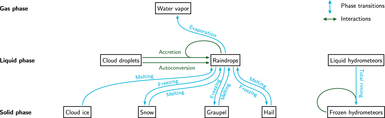
Bulk parameterization schemes describe cloud microphysical properties within each model grid volume with statistical bulk quantities, i.e., moments of the size distribution functions of distinct hydrometeor categories. The two-moment microphysics scheme (Seifert and Beheng, Reference Seifert and Beheng2006) parameterizes cloud microphysics with prognostic number concentrations and mass mixing ratios of cloud droplets, raindrops, cloud ice, snow, graupel, and hail, corresponding to the first two moments of the respective size distribution functions. MPRs describe a change in the prognostic variables through phase transitions and interaction processes (Figure 2). (In this work, we only consider process rates related to a change in the mass mixing ratio.) Here, we consider two warm-rain processes, which both describe an increase in the rain mass mixing ratio through the formation of raindrops from coalescing cloud droplets (autoconversion) and cloud droplets and raindrops (accretion). Evaporation of rain causes a decrease in rainwater mass. Rain mass also decreases by freezing of rain to snow, graupel, and hail at temperatures
$ T<0{}^{\circ}\mathrm{C} $
 . At
$ T>0{}^{\circ}\mathrm{C} $
. At
$ T>0{}^{\circ}\mathrm{C} $
 , all frozen hydrometeors can melt to rain, leading to an increase in the rain mass mixing ratio. Furthermore, we consider riming, whereby liquid particles freeze upon contact with a frozen hydrometeor. The riming rate comprises eight individual processes between each category of hydrometeors in the liquid and solid phase. The melting, freezing, and riming rates represent the sum of all individual processes. As inputs to the ML models, we use mass mixing ratios and number concentrations together with temperature, pressure, and density. (These are listed in the Supplementary Material A.2. A short discussion of exchangeability can be found in Supplementary Material A.3.)
Schematic of selected microphysical processes (arrows) between the six hydrometeor categories (boxes) and water vapor in the two-moment microphysics scheme of Seifert and Beheng (Reference Seifert and Beheng2006). Horizontal (green) arrows represent interaction processes, vertical (blue) arrows represent phase transitions. For simplicity, riming is shown separately. If a process occurs more than once, arrows represent contributions to the total process rate. From an ML perspective, boxes represent input features (mass mixing ratios and number concentrations) and arrows represent targets (process rates).
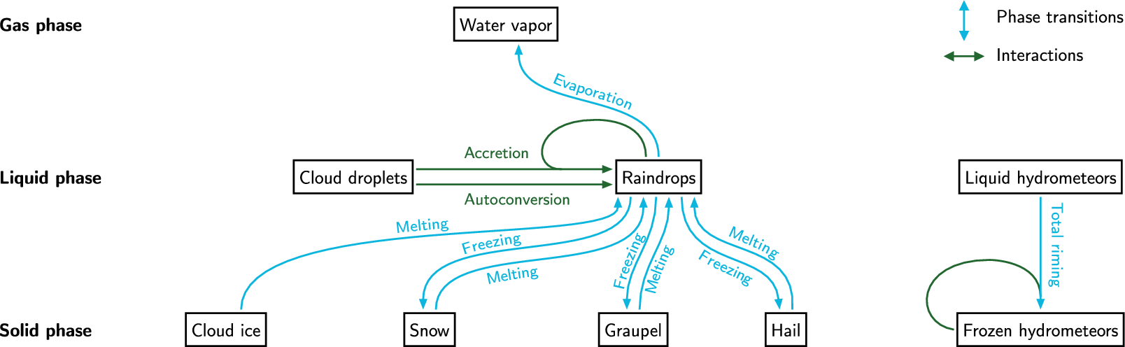
Figure 2. Long description
The flowchart is organized into three vertical tiers.
At the top, the Gas phase contains a box for Water vapor.
In the middle, the Liquid phase contains boxes for Cloud droplets and Raindrops. Two horizontal green arrows point from Cloud droplets to Raindrops, labeled Accretion and Autoconversion. A curved green arrow loops from Raindrops back to itself. A blue arrow labeled Evaporation points from Raindrops up to Water vapor.
At the bottom, the Solid phase contains four boxes: Cloud ice, Snow, Graupel, and Hail. Blue arrows represent phase transitions between these and the liquid phase:
* A blue arrow labeled Melting points from Cloud ice to Raindrops.
* Two blue arrows connect Snow and Raindrops, labeled Freezing (upward) and Melting (downward).
* Two blue arrows connect Graupel and Raindrops, labeled Freezing (upward) and Melting (downward).
* Two blue arrows connect Hail and Raindrops, labeled Freezing (upward) and Melting (downward).
On the far right, a separate simplified diagram shows a box for Liquid hydrometeors above a box for Frozen hydrometeors. A blue arrow labeled Total riming points downward from liquid to frozen, and a curved green arrow loops from the Frozen hydrometeors box back to itself.
A legend in the top right corner identifies blue vertical arrows as Phase transitions and green horizontal arrows as Interactions.
3.2. ICON model simulations and sampling procedure
For training, calibration, and evaluation, we use a dataset compiled from simulation output of the ICON model (version 2.6.6) (Zängl et al., Reference Zängl, Reinert, Rípodas and Baldauf2015) in a limited-area configuration with
$ \overline{\Delta x}\approx 2 $
 km effective grid spacing. The simulations are performed with the two-moment microphysics scheme (Seifert and Beheng, Reference Seifert and Beheng2006) with a fast-physics timestep
$ {\mathrm{t}}_{\mathrm{fast}}=20\hskip0.1em \mathrm{s} $
km effective grid spacing. The simulations are performed with the two-moment microphysics scheme (Seifert and Beheng, Reference Seifert and Beheng2006) with a fast-physics timestep
$ {\mathrm{t}}_{\mathrm{fast}}=20\hskip0.1em \mathrm{s} $
 . The modeling domain extends from
$ -0.4{}^{\circ} $
. The modeling domain extends from
$ -0.4{}^{\circ} $
 W to
$ 17.7{}^{\circ} $
W to
$ 17.7{}^{\circ} $
 E and from
$ 43.7{}^{\circ} $
E and from
$ 43.7{}^{\circ} $
 N to
$ 57.26{}^{\circ} $
N to
$ 57.26{}^{\circ} $
 N, corresponding to the operational ICON-D2 configuration (Reinert et al., Reference Reinert, Prill, Frank, Denhard, Baldauf, Schraff, Gebhardt, Marsigli, Förstner, Zängl, Schlemmer, Blahak and Welzbacher2025). Each vertical column contains 65 levels up to 22 km above ground. The dataset comprises 19 one-day simulations (24 hours each) from January 2022 to July 2023 with an output time step of 10 minutes. We perform simulations for 1 day for each month. For training purposes, the MPRs are added as additional output variables in our setup. Further details on the model configuration are given in Supplementary Material A.1. The set of input features for each target variable is aligned with the computation of the process rate in the ICON subroutine and listed in Supplementary Material B.1. The size of the initial dataset is reduced by random sampling of model grid points. Furthermore, the output from high altitudes is discarded under the assumption that they are cloud-free. We use the simulation output for 2022 for training (even-numbered months) and validation (odd-numbered months); the simulated days for 2023 are used for the test dataset. The training dataset is randomly split into the proper training and the calibration set. The datasets for each target MPR are retrieved from these initial datasets by filtering out all grid points where the value of the MPR fulfills
$ \left|\mathrm{MPR}\right|\ge {10}^{-12}\hskip0.1em \mathrm{kg}\;{\mathrm{kg}}^{-1}\hskip0.1em {{\mathrm{t}}_{\mathrm{fast}}}^{-1} $
N, corresponding to the operational ICON-D2 configuration (Reinert et al., Reference Reinert, Prill, Frank, Denhard, Baldauf, Schraff, Gebhardt, Marsigli, Förstner, Zängl, Schlemmer, Blahak and Welzbacher2025). Each vertical column contains 65 levels up to 22 km above ground. The dataset comprises 19 one-day simulations (24 hours each) from January 2022 to July 2023 with an output time step of 10 minutes. We perform simulations for 1 day for each month. For training purposes, the MPRs are added as additional output variables in our setup. Further details on the model configuration are given in Supplementary Material A.1. The set of input features for each target variable is aligned with the computation of the process rate in the ICON subroutine and listed in Supplementary Material B.1. The size of the initial dataset is reduced by random sampling of model grid points. Furthermore, the output from high altitudes is discarded under the assumption that they are cloud-free. We use the simulation output for 2022 for training (even-numbered months) and validation (odd-numbered months); the simulated days for 2023 are used for the test dataset. The training dataset is randomly split into the proper training and the calibration set. The datasets for each target MPR are retrieved from these initial datasets by filtering out all grid points where the value of the MPR fulfills
$ \left|\mathrm{MPR}\right|\ge {10}^{-12}\hskip0.1em \mathrm{kg}\;{\mathrm{kg}}^{-1}\hskip0.1em {{\mathrm{t}}_{\mathrm{fast}}}^{-1} $
 and
$ {\sum}_k{q}_k\ge {10}^{-12}\hskip0.1em \mathrm{kg}\;{\mathrm{kg}}^{-1} $
and
$ {\sum}_k{q}_k\ge {10}^{-12}\hskip0.1em \mathrm{kg}\;{\mathrm{kg}}^{-1} $
 over all mass mixing ratios
$ {q}_k $
over all mass mixing ratios
$ {q}_k $
 in the set of input features, which corresponds to the threshold
$ {q}_{\mathrm{crit}}={10}^{-12}\hskip0.1em \mathrm{kg}\;{\mathrm{kg}}^{-1} $
in the set of input features, which corresponds to the threshold
$ {q}_{\mathrm{crit}}={10}^{-12}\hskip0.1em \mathrm{kg}\;{\mathrm{kg}}^{-1} $
 in the two-moment microphysics scheme. (In the ICON model,
$ {q}_{\mathrm{crit}} $
in the two-moment microphysics scheme. (In the ICON model,
$ {q}_{\mathrm{crit}} $
 is a critical mass mixing ratio threshold used in the parameterization of certain processes, such as autoconversion.) This allows us to train the regression models to predict logarithmically transformed targets, as the range of the target variables spans multiple orders of magnitude. Thus, the proper training dataset contains
$ 1.12\times {10}^7 $
is a critical mass mixing ratio threshold used in the parameterization of certain processes, such as autoconversion.) This allows us to train the regression models to predict logarithmically transformed targets, as the range of the target variables spans multiple orders of magnitude. Thus, the proper training dataset contains
$ 1.12\times {10}^7 $
 samples, and each validation, calibration, and evaluation dataset contains
$ 1.6\times {10}^6 $
samples, and each validation, calibration, and evaluation dataset contains
$ 1.6\times {10}^6 $
 samples, corresponding to a 70%/10%/10%/10% split. The input features are scaled to the range
$ \left[0,1\right] $
samples, corresponding to a 70%/10%/10%/10% split. The input features are scaled to the range
$ \left[0,1\right] $
 with min-max scaling.
3.3. Training and calibration
A separate model is trained for each process rate. In order to obtain prediction intervals with SCP, we train random forest (RF), gradient boosting (XGB), and neural network (NN) models to obtain point predictions for the process rates. For this, we use the scikit-learn library for the RF models (Pedregosa et al., Reference Pedregosa, Varoquaux, Gramfort, Michel, Thirion, Grisel, Blondel, Prettenhofer, Weiss, Dubourg, Vanderplas, Passos, Cournapeau, Brucher, Perrot and Duchesnay2011), the XGBoost library (Chen and Guestrin, Reference Chen and Guestrin2016) for the XGB models, and PyTorch (Paszke et al., Reference Paszke, Gross, Massa, Lerer, Bradbury, Chanan, Killeen, Lin, Gimelshein, Antiga, Desmaison, Köpf, Yang, DeVito, Raison, Tejani, Chilamkurthy, Steiner, Fang, Bai and Chintala2019) for the NN models. Calibration is performed with the absolute error residual (2.2) and
$ \alpha =0.1 $
 . For CQR, we employ three QR architectures: quantile RF (QRF) models using quantile_forest’s RandomForestQuantileRegressor (Meinshausen, Reference Meinshausen2006; Johnson, Reference Johnson2024), quantile gradient boosting (QXGB), and quantile feed-forward neural networks (QNN). We use the Adam optimizer (Kingma and Ba, Reference Kingma and Ba2017) for training the QNN with a learning rate scheduler with a minimum learning rate of
$ {10}^{-6} $
. For CQR, we employ three QR architectures: quantile RF (QRF) models using quantile_forest’s RandomForestQuantileRegressor (Meinshausen, Reference Meinshausen2006; Johnson, Reference Johnson2024), quantile gradient boosting (QXGB), and quantile feed-forward neural networks (QNN). We use the Adam optimizer (Kingma and Ba, Reference Kingma and Ba2017) for training the QNN with a learning rate scheduler with a minimum learning rate of
$ {10}^{-6} $
 . The maximum number of epochs is 150. The QNN is trained with the quantile loss (Koenker and Bassett, Reference Koenker and Bassett1978), frequently also referred to as the pinball loss,

where
$ \hat{y} $
 is the model’s prediction of the “true”
$ y $
is the model’s prediction of the “true”
$ y $
 . All three QR models are trained to predict the
$ 5\% $
. All three QR models are trained to predict the
$ 5\% $
 - and
$ 95\% $
- and
$ 95\% $
 -quantiles. More details on the training and the model hyperparameters are given in Supplementary Material B.2. The predicted upper and lower quantiles are calibrated with the nonconformity score function (2.6) and
$ \alpha =0.1 $
-quantiles. More details on the training and the model hyperparameters are given in Supplementary Material B.2. The predicted upper and lower quantiles are calibrated with the nonconformity score function (2.6) and
$ \alpha =0.1 $
 .
.
4. Results
4.1. Deterministic performance of microphysical process rate emulation
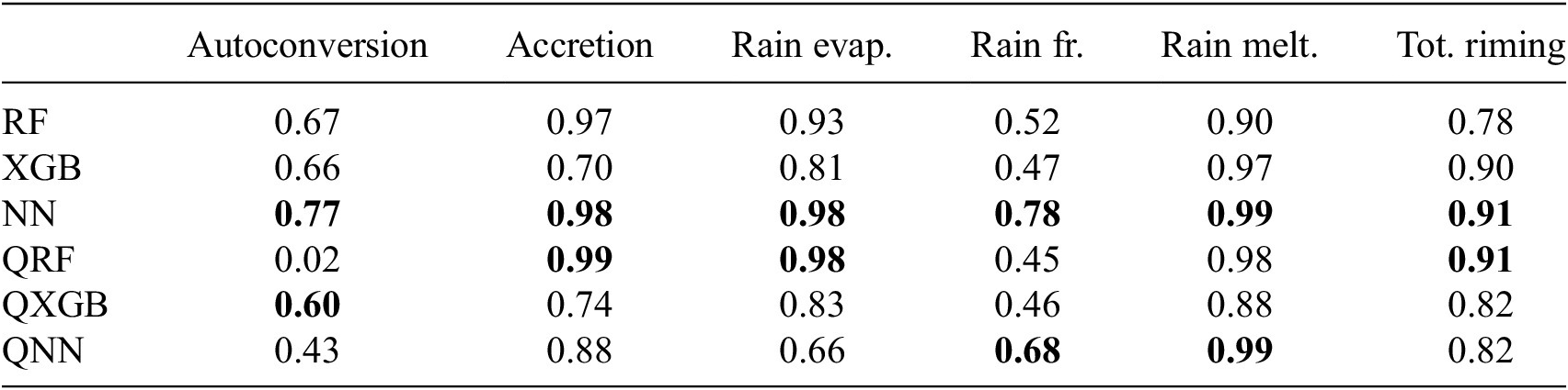
The performance of the deterministic RF, XGB, and NN models is evaluated with the coefficient of determination
$ {R}^2 $
 (Table 1). In order to obtain an estimate of the performance of the QR models, we compute the
$ {R}^2 $
(Table 1). In order to obtain an estimate of the performance of the QR models, we compute the
$ {R}^2 $
 score with the median of the predicted (uncalibrated) upper and lower quantiles. The deterministic models show moderate to high
$ {R}^2 $
score with the median of the predicted (uncalibrated) upper and lower quantiles. The deterministic models show moderate to high
$ {R}^2 $
 scores ranging from
$ 0.47 $
scores ranging from
$ 0.47 $
 to
$ 0.99 $
to
$ 0.99 $
 , with the NN models achieving the highest
$ {R}^2 $
, with the NN models achieving the highest
$ {R}^2 $
 scores for all MPRs. The lowest score is obtained for rain freezing with the XGB model. The QR models yield
$ {R}^2 $
scores for all MPRs. The lowest score is obtained for rain freezing with the XGB model. The QR models yield
$ {R}^2 $
 scores that are largely comparable to those of the deterministic models. An exception is the QRF model for autoconversion, where
$ {R}^2\approxeq 0.02 $
scores that are largely comparable to those of the deterministic models. An exception is the QRF model for autoconversion, where
$ {R}^2\approxeq 0.02 $
 . For all other QR models and process rates,
$ {R}^2 $
. For all other QR models and process rates,
$ {R}^2 $
 ranges from
$ 0.43 $
ranges from
$ 0.43 $
 to
$ 0.99 $
to
$ 0.99 $
 .
.
Deterministic performance in terms of the
$ {R}^2 $
 score
score
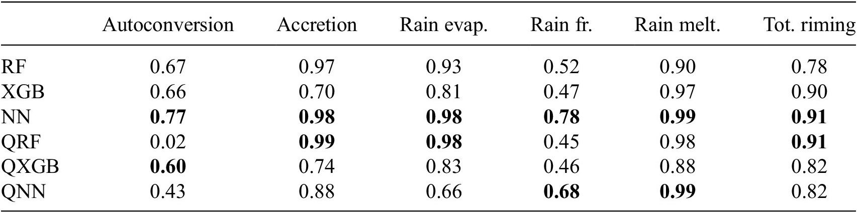
Table 1. Long description
The table consists of seven columns and seven rows. The columns are labeled: Model Type, Autoconversion, Accretion, Rain evap. (evaporation), Rain fr. (freezing), Rain melt. (melting), and Tot. riming (Total riming).
* R F: 0.67, 0.97, 0.93, 0.52, 0.90, 0.78.
* X G B: 0.66, 0.70, 0.81, 0.47, 0.97, 0.90.
* N N: 0.77, 0.98, 0.98, 0.78, 0.99, 0.91. (Highest scores in all categories for deterministic models).
* Q R F: 0.02, 0.99, 0.98, 0.45, 0.98, 0.91.
* Q X G B: 0.60, 0.74, 0.83, 0.46, 0.88, 0.82.
* Q N N: 0.43, 0.88, 0.66, 0.68, 0.99, 0.82.
Bolded values indicate the highest performance for deterministic and Q R models respectively. N N consistently shows high performance across most processes, while Q R F and Q N N share top scores in specific categories like Accretion and Rain melting.
Note: The scores for the QR models are computed with the median of the predicted uncalibrated upper and lower quantiles. For each process rate, the highest score for the deterministic and QR models is highlighted in bold.
4.2. Conformal prediction uncertainty estimates
We evaluate the calibration of the CP intervals with the prediction interval coverage probability (PICP)

which is the proportion of the true values that are covered by the prediction intervals, i.e., the PICP evaluates the marginal coverage property (2.1). Here,
$ n $
 is the size of the test set,
$ {Y}_i $
is the size of the test set,
$ {Y}_i $
 the true value, and
$ \mathcal{C}\left({X}_i\right) $
the true value, and
$ \mathcal{C}\left({X}_i\right) $
 the prediction interval. With
$ \alpha =0.1 $
the prediction interval. With
$ \alpha =0.1 $
 , we aim for
$ \mathrm{PICP}\approx 90\% $
, we aim for
$ \mathrm{PICP}\approx 90\% $
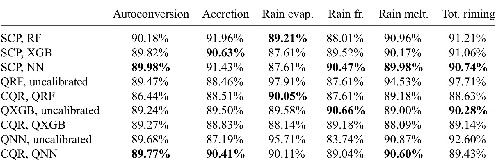
 . The results are given in Table 2; for comparison, we include the PICP for the uncalibrated prediction intervals obtained with the QR models. We find that the
$ \mathrm{PICP}\approx 90\% $
. The results are given in Table 2; for comparison, we include the PICP for the uncalibrated prediction intervals obtained with the QR models. We find that the
$ \mathrm{PICP}\approx 90\% $
 for both the deterministic models calibrated with SCP and the CQR models. Yet, in some cases, the PICP falls slightly below the target
$ 90\% $
for both the deterministic models calibrated with SCP and the CQR models. Yet, in some cases, the PICP falls slightly below the target
$ 90\% $
 . This may be due to sampling variability but it could also indicate mild violations of the exchangeability assumption. Furthermore, we observe that calibration does not always result in a PICP that is closer to 90%, compared to the uncalibrated intervals. This can be seen, for instance, for autoconversion and the QRF model or accretion and the QXGB model. In these cases, calibration decreases the PICP slightly. This can occur because the CQR nonconformity score function (2.6) can be negative and thus shrink the predicted interval, as the score function is designed to account for both undercoverage and overcoverage (Romano et al., Reference Romano, Patterson and Candes2019). Nevertheless, in other cases we observe a significant improvement, for example with the QRF models for the melting to rain and total riming rate.
Prediction interval coverage probability (PICP)
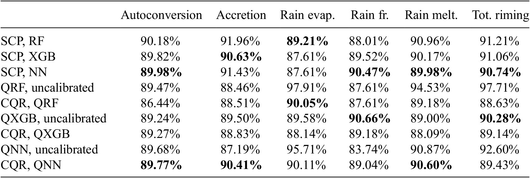
Table 2. Long description
The table consists of 9 rows of models and 6 columns of process rates. The columns are Autoconversion, Accretion, Rain evaporation, Rain freezing, Rain melting, and Total riming.
Row 1: S C P, R F shows values from 88.01 percent to 91.96 percent, with 89.21 percent bolded for Rain evaporation.
Row 2: S C P, XGB shows values from 87.61 percent to 91.06 percent, with 90.63 percent bolded for Accretion.
Row 3: S C P, N N shows values from 87.61 percent to 91.43 percent, with bolded values for Autoconversion 89.98 percent, Rain freezing 90.47 percent, Rain melting 89.98 percent, and Total riming 90.74 percent.
Row 4: Q R F, uncalibrated (in gray) shows values from 87.61 percent to 97.91 percent.
Row 5: C Q R, Q R F shows values from 86.44 percent to 90.05 percent, with 90.05 percent bolded for Rain evaporation.
Row 6: Q X G B, uncalibrated (in gray) shows values from 89.00 percent to 90.66 percent, with bolded values for Rain freezing 90.66 percent and Total riming 90.28 percent.
Row 7: C Q R, Q X G B shows values from 88.09 percent to 89.27 percent.
Row 8: Q N N, uncalibrated (in gray) shows values from 83.74 percent to 95.71 percent.
Row 9: C Q R, Q N N shows values from 89.04 percent to 90.60 percent, with bolded values for Autoconversion 89.77 percent, Accretion 90.41 percent, and Rain melting 90.60 percent.
Bolded values indicate the best P I C P, defined as the minimum absolute difference from 90 percent.
Note: For comparison, we show the results for the uncalibrated prediction intervals obtained with QR in gray. For each process rate, the best PICP obtained with SCP and CQR is highlighted in bold, which is defined as
$ \min \left(|\mathrm{PICP}-90\%|\right). $

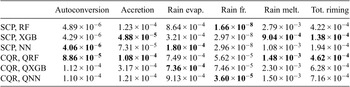
The sharpness of the prediction intervals is evaluated with the normalized mean prediction interval width (NMPIW):

where
$ U $
 and
$ L $
and
$ L $
 refer to the calibrated upper and lower prediction interval bounds. We present the results in Table 3. (Note that the length of the calibrated and uncalibrated prediction intervals is similar in each case, therefore, we do not include both results.) We find that for each process rate, the smallest NMPIW is obtained with SCP. For accretion, rain evaporation, rain melting, and total riming, the NMPIW values obtained with SCP with the deterministic models and CQR with the QR models differ by not more than one order of magnitude for each MPR. Yet, for autoconversion and rain freezing, the NMPIW obtained with SCP is smaller by up to two and three orders of magnitude, respectively. Moreover, a higher PICP does not necessarily imply a larger or smaller NMPIW, as can be seen, e.g., for the rain freezing and the total riming rate, where the smallest NMPIW values correspond to neither the highest nor lowest PICP.
Normalized mean prediction interval width (NMPIW)
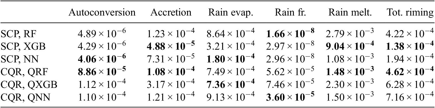
Table 3. Long description
The table consists of seven columns. The first column is unlabeled and contains model pairs. The subsequent six columns are atmospheric processes: Autoconversion, Accretion, Rain evap. (evaporation), Rain fr. (freezing), Rain melt. (melting), and Tot. (total) riming.
Row 1: S C P, R F. Values are 4.89 times 10 super minus 6, 1.23 times 10 super minus 4, 8.64 times 10 super minus 4, bold 1.66 times 10 super minus 8, 2.79 times 10 super minus 3, and 4.22 times 10 super minus 4.
Row 2: S C P, X G B. Values are 4.29 times 10 super minus 6, bold 4.88 times 10 super minus 5, 3.21 times 10 super minus 4, 2.97 times 10 super minus 8, bold 9.04 times 10 super minus 4, and bold 1.38 times 10 super minus 4.
Row 3: S C P, N N. Values are bold 4.06 times 10 super minus 6, 7.31 times 10 super minus 5, bold 1.80 times 10 super minus 4, 2.96 times 10 super minus 8, 1.08 times 10 super minus 3, and 1.94 times 10 super minus 4.
Row 4: C Q R, Q R F. Values are bold 8.86 times 10 super minus 5, bold 1.08 times 10 super minus 4, 7.49 times 10 super minus 4, 5.62 times 10 super minus 5, bold 1.48 times 10 super minus 3, and bold 4.62 times 10 super minus 4.
Row 5: C Q R, Q X G B. Values are 1.12 times 10 super minus 4, 3.17 times 10 super minus 4, bold 7.36 times 10 super minus 4, 7.46 times 10 super minus 5, 2.30 times 10 super minus 3, and 6.28 times 10 super minus 4.
Row 6: C Q R, Q N N. Values are 1.10 times 10 super minus 4, 1.21 times 10 super minus 4, 9.13 times 10 super minus 4, bold 3.60 times 10 super minus 5, 1.50 times 10 super minus 3, and 7.16 times 10 super minus 4.
Bold values indicate the smallest N M P I W obtained within the S C P and C Q R groups for each process.
Note: For each process rate, the smallest NMPIW obtained with SCP and CQR, is highlighted in bold.
We visualize the prediction intervals derived with SCP and CQR exemplarily for autoconversion in Figure 3. (Additional results for all process rates are included in the Supplementary Material C.) It is apparent that the SCP results mainly depend on
$ {Q}_{1-\alpha } $
 . For true values smaller than
$ {Q}_{1-\alpha } $
. For true values smaller than
$ {Q}_{1-\alpha } $
 , all prediction intervals have the same width and mostly cover the true value. Above
$ {Q}_{1-\alpha } $
, all prediction intervals have the same width and mostly cover the true value. Above
$ {Q}_{1-\alpha } $
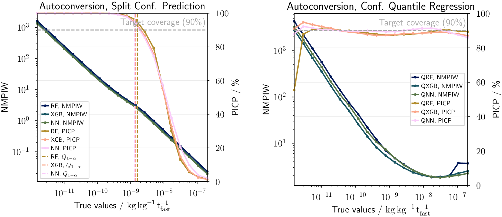
 , this is not the case anymore, with prediction intervals with decreasing PICP typically missing the true value of the MPR. In contrast, with CQR, valid prediction intervals are present across the full range of true values. This indicates that in our case, single-valued evaluation metrics might not be reflective of the true behavior. To further investigate the dependence of the PICP and NMPIW on the size range of the target variables, in Figure 4, we show both quantities binned by the size of the true value for SCP and CQR, respectively. Consistent with Figure 3, we observe that with SCP, the PICP is almost at 100% for size bins of the true values below
$ {Q}_{1-\alpha } $
, this is not the case anymore, with prediction intervals with decreasing PICP typically missing the true value of the MPR. In contrast, with CQR, valid prediction intervals are present across the full range of true values. This indicates that in our case, single-valued evaluation metrics might not be reflective of the true behavior. To further investigate the dependence of the PICP and NMPIW on the size range of the target variables, in Figure 4, we show both quantities binned by the size of the true value for SCP and CQR, respectively. Consistent with Figure 3, we observe that with SCP, the PICP is almost at 100% for size bins of the true values below
$ {Q}_{1-\alpha } $
 and drops to
$ \mathrm{PICP}\ll 90\% $
and drops to
$ \mathrm{PICP}\ll 90\% $
 above
$ {Q}_{1-\alpha } $
above
$ {Q}_{1-\alpha } $
 . With CQR, the PICP is approximately 90% across all size bins, in agreement with Figure 3. With both methods, the NMPIW decreases with increasing size of the target value. Thus, unlike SCP, CQR can predict state-dependent intervals across the entire range of MPRs, yielding more reliable prediction intervals in general. (Supplementary Material C.3 includes an analysis of the absolute residuals, which is a diagnostic for heteroscedasticity.)
Calibrated prediction intervals with SCP and the NN (left) and CQR and the QNN (right) for autoconversion. For better visualization, we only show 1500 randomly selected samples.
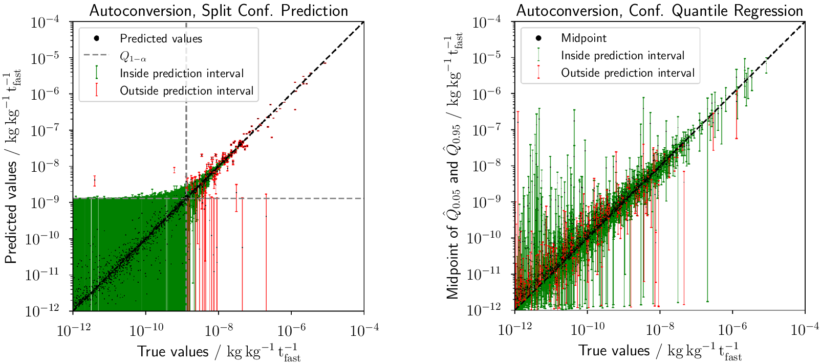
Figure 3. Long description
A two-panel scatter plot on logarithmic scales. Both panels feature an x-axis labeled True values / k g k g sub -1 t sub fast super -1 and a diagonal dashed line representing a perfect one-to-one match.
Left Panel: Titled Autoconversion, Split Conf. Prediction. The y-axis is labeled Predicted values / k g k g sub -1 t sub fast super -1. Data points are concentrated along the diagonal. Green vertical bars represent points inside the prediction interval, dominating the lower-left quadrant below 10 super -9. Red vertical bars represent points outside the prediction interval, appearing more frequently as values increase. A horizontal and vertical dashed line intersect at approximately 10 super -9.
Right Panel: Titled Autoconversion, Conf. Quantile Regression. The y-axis is labeled Midpoint of Q hat sub 0.05 and Q hat sub 0.95 / k g k g sub -1 t sub fast super -1. Black dots represent the midpoint. Green and red vertical error bars are distributed across the entire range from 10 super -12 to 10 super -4. Unlike the left panel, the prediction intervals in this C Q R plot vary significantly in length across the entire data range, with a high density of green bars following the diagonal trend.
Normalized mean prediction interval width (NMPIW) and prediction interval coverage probability (PICP) binned by value of the autoconversion rate for SCP (left) and CQR (right).
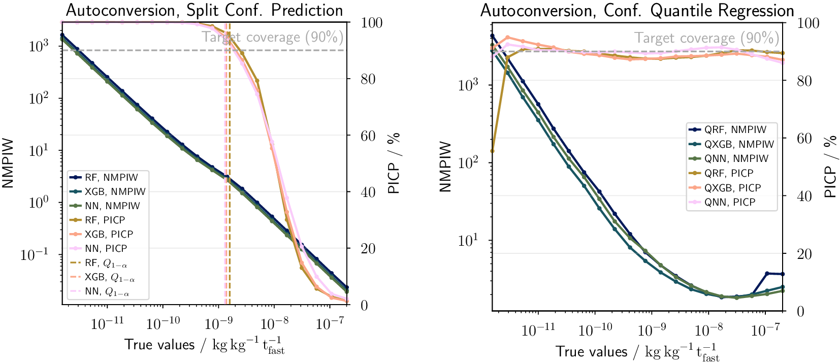
Figure 4. Long description
A two-panel figure with logarithmic x-axes and dual y-axes. The x-axis for both panels is True values / kg kg super -1 t sub fast. The left y-axis is N M P I W on a log scale from 10 super -1 to 10 super 3. The right y-axis is P I C P / % from 0 to 100. A horizontal dashed line at 90% indicates Target coverage.
Left Panel: Autoconversion, Split Conf. Prediction (S C P).
- N M P I W for R F, X G B, and N N shows a steep linear decrease from 10 super 3 to 10 super -1 as true values increase.
- P I C P for all three models remains stable at 100% until true values reach approximately 10 super -9, after which it drops sharply toward 0%.
- Vertical dashed lines indicate Q sub 1 minus alpha thresholds for each model near 10 super -9.
Right Panel: Autoconversion, Conf. Quantile Regression (C Q R).
- N M P I W for Q R F, Q X G B, and Q N N follows a U-shaped curve, starting high at 10 super 3, dipping to a minimum near 10 super -8, and slightly increasing at the highest true values.
- P I C P for all models remains consistently high, fluctuating slightly around the 90% target coverage line across the entire range of true values.
Legends in both panels identify R F (Random Forest), X G B (X G Boost), and N N (Neural Network) variants for both metrics.
5. Conclusions
We applied and evaluated conformal methods to derive calibrated prediction intervals for microphysical process rates (MPRs), enabling the retrieval of detailed process information from high-resolution atmospheric simulations. We compared split conformal prediction, which is simple and inexpensive, with conformalized quantile regression, which requires training a quantile regression model. Applied to well-performing machine learning emulators, both approaches yield satisfactory results for calibration (measured with PICP) and sharpness (measured with NMPIW) on average. In certain cases, the PICP falls slightly below the nominal level, which might indicate mild violations of the exchangeability assumption. Moreover, split conformal prediction exhibits a strongly bin-dependent PICP and unreliable intervals for process rate values exceeding
$ {Q}_{1-\alpha } $
 . In contrast, conformalized quantile regression adapts to heteroscedasticity and thus better reflects the distribution of MPRs, making it the preferable approach when large values are most important. Future work could explore alternative nonconformity scores (Papadopoulos et al., Reference Papadopoulos, Gammerman and Vovk2008; Lei et al., Reference Lei, G’Sell, Rinaldo, Tibshirani and Wasserman2018; Gopakumar et al., Reference Gopakumar, Gray, Oskarsson, Zanisi, Giles, Kusner, Pamela and Deisenroth2026) and loss functions for quantile regression training (e.g., Feldman et al., Reference Feldman, Bates and Romano2021) to further improve efficient, reliable uncertainty quantification across the diverse distributions encountered in weather and climate science.
Supplementary material
The supplementary material for this article can be found at http://doi.org/10.1017/eds.2026.10051.
Acknowledgments
The authors gratefully acknowledge the computing time provided on the high-performance computer HoreKa by the National High-Performance Computing Center at KIT (NHR@KIT). This center is jointly supported by the Federal Ministry of Education and Research and the Ministry of Science, Research, and the Arts of Baden-Württemberg, as part of the National High-Performance Computing (NHR) joint funding program (https://www.nhr-verein.de/en/our-partners). HoreKa is partly funded by the German Research Foundation (DFG). The GitHub Copilot extension for Visual Studio Code and ChatGPT-5.2 was used to support the development of the model code. Generative AI tools have only been used for proofreading; not for text preparation. Supplementary Figures 4, 7, 8, 9, and 10 make use of the Scientific color maps 7.0 (Crameri et al., Reference Crameri, Shephard and Heron2020). Figures 1 and 2 were created using the LaTeX package TikZ (Tantau, Reference Tantau2025).
Author contribution
Conceptualization: M.S., T.B., C.H.; Data curation: M.S.; Data visualization: M.S.; Methodology: M.S.; Writing original draft: M.S.; Writing review & editing: M.S., T.B., C.H. All authors approved the final submitted draft.
Data availability statement
The released version of the data and code necessary to reproduce the manuscript’s figures are publicly available on Zenodo at https://zenodo.org/records/19114006 (DOI: https://doi.org/10.5281/zenodo.19114006) and in the GitHub repository https://github.com/miriamsimm/ConformalMPR. The trained models as well as the ICON model simulation output are available upon request. The newest version of the source code that was used to perform the simulations with the ICON model can be found at icon-model.org.
Funding statement
M. S. and C. H. acknowledge funding from the NHR Call for Collaboration Project MICRO. C. H. acknowledges funding from the European Union’s Horizon Europe Programme under Grant Agreement No. 101137639 (CleanCloud). T. B. acknowledges funding from the Swiss State Secretariat for Education, Research and Innovation (SERI) for the Horizon Europe project AI4PEX (Grant agreement ID: 101137682 and SERI no 23.00546).
Competing interests
The authors declare none.
Ethics statement
The research meets all ethical guidelines, including adherence to the legal requirements of the study country.
Provenance statement
This article is part of the Climate Informatics 2026 proceedings and was accepted in Environmental Data Science on the basis of the Climate Informatics peer review process.




 Open access

