


I. Introduction
Collective models of intra-household consumption decisions in the tradition of Chiappori (Reference Chiappori1988), surveyed by Chiappori and Mazzocco (Reference Chiappori and Mazzocco2017), are designed to reflect opportunities for intra-household risk sharing for couples that are absent from traditional, unitary models for a single agent. Recent literature provides evidence that unitary models are missing elements of intra-household decision-making that are important to explain financial risk-taking decisions of couples (Ke (Reference Ke2021), (Reference Ke2025), Guiso and Zaccaria (Reference Guiso and Zaccaria2023)). Our article contributes to a small but evolving literature proposing collective models of portfolio choice.Footnote 1 We extend the dynamic model proposed by Mazzocco (Reference Mazzocco2004) and reviewed in Browning, Chiappori, and Weiss (Reference Browning, Chiappori and Weiss2014) to incorporate the life-cycle portfolio choice decisions of dual-income couples.
Efficient risk sharing implies a consumption-sharing rule that optimally allocates household consumption across partners such that the ratio of their marginal utilities of private consumption remains constant over the life cycle. We focus on risk sharing that results from intra-household heterogeneity in risk preferences. Intuitively, the less risk-averse partner provides partial downside consumption insurance for the more risk-averse partner, who, in return, gives up some of the upside potential in consumption. Importantly, the risk-sharing channel differs from diversifying earnings risk in dual-income couples. Unlike risk diversification, risk sharing affects both single-income and dual-income couples, provided that partners differ in relative risk aversion.
Using a calibrated, collective life-cycle portfolio choice model, we find surprisingly large economic effects of risk sharing on portfolio choice. For example, a mean-preserving spread in the partners’ coefficients of relative risk aversion from 5 for both partners to 2 and 8 increases their average risky asset share by 25% across the life cycle. Importantly, we show that risk sharing has a larger economic impact on portfolio choice than risk diversification. While unitary models usually do not generate the same portfolio choice outcomes as collective models, we show that a unitary model with an appropriately constructed relative risk aversion coefficient generates similar predictions to collective models for moderate background risk. Finally, we provide strong empirical support for our key finding that financial risk-taking increases with the potential to share risk within the household.
In the collective model, the couple solves a Pareto problem which consists of maximizing a weighted average of the individual value functions of the partners subject to a household budget constraint. We assume that the partners have power utility in individual consumption.Footnote 2 The Pareto weights reflect the relative bargaining power of the partners.Footnote 3 In its most general form, our model allows for intra-household heterogeneity in bargaining power, risk preferences, discount factors, and conditional survival probabilities. To concentrate on differences in risk preferences and bargaining power, we assume certain survival probabilities and identical discount factors, following Ortigueira and Siassi (Reference Ortigueira and Siassi2013) and Apps, Andrienko, and Rees (Reference Apps, Andrienko and Rees2014). Unlike these studies, however, we emphasize the portfolio choice implications of intra-household risk sharing.
The partners also differ in their earnings process parameters. We extend the earnings process of Kaplan (Reference Kaplan2012) to a dual-income couple. Unlike earlier dual-income processes proposed by Shore (Reference Shore2015) and Blundell, Pistaferri, and Saporta-Eksten (Reference Blundell, Pistaferri and Saporta-Eksten2016), our model allows for persistent but nonpermanent individual earnings shocks. The partners’ persistent earnings shocks are allowed to be correlated with each other and with the innovations to stock excess returns. We estimate the earnings process from the Panel Study of Income Dynamics (PSID). According to our estimates, male partners experience more persistent but less volatile earnings shocks than female partners.
Like Hertzberg (Reference Hertzberg2024), we assume that household formation is exogenous and that the partners stay together for their entire adult lives. Correspondingly, we assume that the partners fully commit to implementing the ex ante optimal saving and portfolio choice outcomes of the model. In this case, the Pareto weights are age-invariant, reflecting the partners’ decision power at the time of household formation.Footnote 4 In models with limited commitment, such as the collective life-cycle portfolio choice model of Addoum, Kung, and Morales (Reference Addoum, Kung and Morales2017), the couple separates if at least one partner is better off as a single in response to a change in relative bargaining power. We acknowledge that full commitment in dynamic models has been rejected in favor of limited commitment (e.g., Mazzocco (Reference Mazzocco2007)) and can change the predictions of our model.Footnote 5 However, better understanding the portfolio choice implications of risk sharing in full-commitment models is a necessary first step before extending the model to account for limited commitment.
Our findings suggest an important role for risk sharing in the portfolio choice decisions of partners who differ in relative risk aversion. Based on simulations from the calibrated life-cycle model, a mean-preserving spread in the partners’ relative risk aversion increases consumption and financial risk-taking across the life cycle. Compared to partners with identical relative risk aversion of 5, partners with relative risk aversion coefficients of 4 and 6 (3 and 7) [2 and 8] on average increase the share of wealth allocated to stocks by 2.3% (10.0%) [24.7%] across the life cycle. Compared to risk sharing, risk diversification has a much smaller effect on portfolio choice. For instance, an extreme increase in the correlation between the partners’ persistent earnings shocks from 0.1 to 0.9 only implies a 2.2% reduction in the risky asset share in a collective model with relative risk aversion coefficients of 3 and 7.
Given these findings, we also analyze the impact of risk sharing on precautionary saving. Apps et al. (Reference Apps, Andrienko and Rees2014) find that precautionary saving increases in the collective model in response to a mean-preserving spread in idiosyncratic earnings risk if individual preferences exhibit prudence. We show that this saving response is more pronounced for couples with fewer opportunities to share risk within the household. For example, partners with risk aversion coefficients of 3 and 7 optimally save more than partners with risk aversion coefficients of 2 and 8. As a result, when we analyze a model with stock market participation costs, the households with higher heterogeneity in risk aversion that save less enter the stock market later in life.
Given the status of the unitary life-cycle portfolio choice model in the tradition of Cocco, Gomes, and Maenhout (Reference Cocco, Gomes and Maenhout2005) as the workhorse model in household finance,Footnote 6 we investigate whether a unitary model can approximate the portfolio choice implications of a collective model when partners differ in risk aversion. In this case, the risk aversion coefficient of the couple in the collective model varies with age as a function of individual consumption shares (see, e.g., Ortigueira and Siassi (Reference Ortigueira and Siassi2013)). This makes it impossible for a unitary model to exactly replicate the solutions of the collective model. However, we show that a unitary model that uses the collective relative risk aversion coefficient proposed by Gu, Peng, and Zhang (Reference Gu, Peng and Zhang2024) can approximate the portfolio choice decisions of the couple in the collective model, provided that background risk is relatively low.
Whether partners differ in relative risk aversion is an empirical question. Using data from the Health and Retirement Study (HRS), Mazzocco (Reference Mazzocco2004) finds that about 48% of couples aged 50+ report differences in the risk preferences of partners. This number reduces to 43% in the Household, Income, and Labour Dynamics in Australia (HILDA) Survey, analyzed by Gu et al. (Reference Gu, Peng and Zhang2024), which includes younger households as well. While most of these observed differences in risk preferences between partners are relatively small, Gu et al. (Reference Gu, Peng and Zhang2024) find that husbands, on average, are not only more risk tolerant than wives (as in Addoum (Reference Addoum2017) and Brooks, Sangiorgi, Hillenbrand, and Money (Reference Brooks, Sangiorgi, Hillenbrand and Money2019)) but also have higher bargaining power. These findings imply substantial increases in risk-taking in our model compared to a unitary model.
While the contribution of our article is mostly normative in nature, we still investigate whether the main empirical implications of the collective life-cycle model with full commitment are reflected in the data. Our simulation results suggest that any empirical analysis of financial risk-taking at the household level in the tradition of Campbell (Reference Campbell2006) should include variables describing the potential to share risk within the household. We use an extended panel of the HILDA data previously employed by Gu et al. (Reference Gu, Peng and Zhang2024) to investigate the relationship between the financial risk-taking of couples and intra-household heterogeneity in risk preferences. Interestingly, we provide empirical evidence that supports our model’s main prediction that intra-household heterogeneity in risk aversion can substantially affect portfolio choice. Specifically, a one-unit increase in the absolute value of the difference in the partners’ risk aversions (for a given mean) increases the share of wealth in stocks by 1.3 percentage points. In a model with stock market participation costs, this also generates a drop in stock market participation ranging between 1.1 and 1.6 percentage points. Quantitatively, these effects are similar to those generated from simulating our model for modest degrees of intra-household heterogeneity in risk aversion.
The existing literature proposing collective portfolio choice models for couples remains silent on the portfolio choice implications of intra-household risk sharing. Previous literature either abstracts from consumption decisions (Gu et al. (Reference Gu, Peng and Zhang2024)), focuses on diversification of earnings risk (Addoum et al. (Reference Addoum, Kung and Morales2017)) or assumes that consumption is equally shared within the household (Love (Reference Love2010), Hong and Ríos-Rull (Reference Hong and Ríos-Rull2012), and Hubener, Maurer, and Mitchell (Reference Hubener, Maurer and Mitchell2015)). Equal sharing of consumption is optimal in the collective model if partners have identical discount factors, bargaining power, and risk preferences. In this case, opportunities for risk sharing are absent, and a unitary model can replicate the solutions of the collective model (Mazzocco (Reference Mazzocco2004)). In our case, partners differ in risk preferences, which creates risk-sharing opportunities with significant portfolio choice implications.
The article is outlined as follows: Section II proposes the collective life-cycle portfolio choice model for a dual-income couple. The model is calibrated, and the earnings process of the couple is estimated from PSID data in Section III. Section IV contains simulation results for the impact of risk sharing on portfolio choice. Section V provides supporting empirical evidence using data from the HILDA Survey, while Section VI concludes.
II. Life-Cycle Portfolio Choice for Couples
We propose a collective life-cycle portfolio choice model for a dual-income couple that decides in every period on individual consumption and the share of wealth invested in risky assets. In an extension below (in Section IV.F), we consider the decision to participate in the stock market in the presence of participation costs. The model implies efficient intra-household risk sharing, which is achieved by a consumption-sharing rule that distributes total household consumption between the two partners. As a result, the couple’s coefficient of relative risk aversion generally varies across the life cycle. We discuss conditions under which a unitary model for a single agent representing the couple can replicate the solutions of the collective model.
A. Budget Constraint and Earnings Process
We consider a dual-income couple composed of partners $ \left(A,B\right) $
of equal age. At every adult age
$ \left(A,B\right) $
of equal age. At every adult age $ t=1,\dots, T $
, the partners receive individual earnings (
$ t=1,\dots, T $
, the partners receive individual earnings ( $ {Y}_{At},{Y}_{Bt} $
) and decide on individual consumption (
$ {Y}_{At},{Y}_{Bt} $
) and decide on individual consumption ( $ {C}_{At},{C}_{Bt} $
) and the share of their joint savings (
$ {C}_{At},{C}_{Bt} $
) and the share of their joint savings ( $ {\alpha}_t $
) that is allocated to the stock market. Following Deaton (Reference Deaton1991), cash-on-hand (
$ {\alpha}_t $
) that is allocated to the stock market. Following Deaton (Reference Deaton1991), cash-on-hand ( $ {X}_t $
) is defined as the sum of financial wealth and household earnings,
$ {X}_t $
) is defined as the sum of financial wealth and household earnings, $ {Y}_t={Y}_{At}+{Y}_{Bt} $
, and evolves according to
$ {Y}_t={Y}_{At}+{Y}_{Bt} $
, and evolves according to
 $$ {X}_t=\left({X}_{t-1}-{C}_{t-1}\right)\left({R}^f+{\alpha}_{t-1}\left({R}_t-{R}^f\right)\right)+{Y}_t. $$
Joint savings, the difference between cash-on-hand and household consumption, $ {C}_t={C}_{At}+{C}_{Bt} $
, are invested in a portfolio consisting of a risk-free asset with a certain real gross return,
$ {C}_t={C}_{At}+{C}_{Bt} $
, are invested in a portfolio consisting of a risk-free asset with a certain real gross return, $ {R}^f $
, and the stock market with risky real gross return,
$ {R}^f $
, and the stock market with risky real gross return, $ {R}_t $
. The couple is assumed to be borrowing and short-sale constrained, which implies
$ {R}_t $
. The couple is assumed to be borrowing and short-sale constrained, which implies $ {\alpha}_t\in \left[0,1\right],\forall t $
. Using
$ {\alpha}_t\in \left[0,1\right],\forall t $
. Using $ {r}_t=\ln \left({R}_t\right) $
and
$ {r}_t=\ln \left({R}_t\right) $
and $ {r}^f=\ln \left({R}^f\right) $
, we assume that the log excess return on stocks is generated by
$ {r}^f=\ln \left({R}^f\right) $
, we assume that the log excess return on stocks is generated by
 $$ {r}_t-{r}^f=\mu +{\nu}_t, $$
where $ \mu $
is the unconditionally expected equity risk premium and
$ \mu $
is the unconditionally expected equity risk premium and $ {\nu}_t $
is an innovation that is
$ {\nu}_t $
is an innovation that is $ \mathrm{IID}. $
normal with mean zero. Investment opportunities are constant.
$ \mathrm{IID}. $
normal with mean zero. Investment opportunities are constant.
We propose a model of earnings dynamics that extends the model of Kaplan (Reference Kaplan2012) to a dual-income household. Assume that the partners’ log earnings consist of a deterministic life-cycle component and a stochastic residual component, such that $ {y}_{At}=\ln \left({Y}_{At}\right)={d}_{At}+{e}_{At} $
and
$ {y}_{At}=\ln \left({Y}_{At}\right)={d}_{At}+{e}_{At} $
and $ {y}_{Bt}=\ln \left({Y}_{Bt}\right)={d}_{Bt}+{e}_{Bt} $
, where
$ {y}_{Bt}=\ln \left({Y}_{Bt}\right)={d}_{Bt}+{e}_{Bt} $
, where
 $$ {e}_{At}={\omega}_A+{\eta}_{At}+{\varepsilon}_{At}\hskip2em {e}_{Bt}={\omega}_B+{\eta}_{Bt}+{\varepsilon}_{Bt} $$
 $$ {\eta}_{At}={\phi}_A{\eta}_{At-1}+{\zeta}_{At}\hskip2em {\eta}_{Bt}={\phi}_B{\eta}_{Bt-1}+{\zeta}_{Bt}. $$
The deterministic components, $ {d}_{At},{d}_{Bt} $
, include quartic polynomials in the partners’ respective ages. Log residual earnings for each partner in equation (3) are decomposed into a persistent component
$ {d}_{At},{d}_{Bt} $
, include quartic polynomials in the partners’ respective ages. Log residual earnings for each partner in equation (3) are decomposed into a persistent component $ \left({\eta}_{At}=\ln \left({Y}_{At}^p\right),{\eta}_{Bt}=\ln \left({Y}_{Bt}^p\right)\right) $
, which follows the first-order Markov process in equation (4), a transitory component
$ \left({\eta}_{At}=\ln \left({Y}_{At}^p\right),{\eta}_{Bt}=\ln \left({Y}_{Bt}^p\right)\right) $
, which follows the first-order Markov process in equation (4), a transitory component $ \left({\varepsilon}_{At},{\varepsilon}_{Bt}\right) $
, and an age-invariant random effect
$ \left({\varepsilon}_{At},{\varepsilon}_{Bt}\right) $
, and an age-invariant random effect $ \left({\omega}_A,{\omega}_B\right) $
. We assume that transitory shocks and random effects are IID normal with zero means and variances
$ \left({\omega}_A,{\omega}_B\right) $
. We assume that transitory shocks and random effects are IID normal with zero means and variances $ \left({\sigma}_{A\varepsilon}^2,{\sigma}_{B\varepsilon}^2\right) $
and
$ \left({\sigma}_{A\varepsilon}^2,{\sigma}_{B\varepsilon}^2\right) $
and $ \left({\sigma}_{A\omega}^2,{\sigma}_{B\omega}^2\right) $
, respectively. We allow the innovations to the persistent earnings components to be correlated with each other, with a correlation coefficient
$ \left({\sigma}_{A\omega}^2,{\sigma}_{B\omega}^2\right) $
, respectively. We allow the innovations to the persistent earnings components to be correlated with each other, with a correlation coefficient $ \rho $
, and with the innovations to the log stock excess return in equation (2) with correlation coefficients
$ \rho $
, and with the innovations to the log stock excess return in equation (2) with correlation coefficients $ \left({\rho}_{A\nu},{\rho}_{B\nu}\right) $
. Specifically, we assume the following multivariate normal distribution for these innovations:
$ \left({\rho}_{A\nu},{\rho}_{B\nu}\right) $
. Specifically, we assume the following multivariate normal distribution for these innovations:
 $$ \left(\begin{array}{c}{\zeta}_{A t}\\ {}{\zeta}_{B t}\\ {}{\nu}_t\end{array}\right)\sim i.i.d.N\left[\left(\begin{array}{c}0\\ {}0\\ {}0\end{array}\right),\left(\begin{array}{ccc}{\sigma}_{A\zeta}^2& {\rho \sigma}_{A\zeta}{\sigma}_{B\zeta}& {\rho}_{A\nu}{\sigma}_{A\zeta}{\sigma}_{\nu}\\ {}{\rho \sigma}_{A\zeta}{\sigma}_{B\zeta}& {\sigma}_{B\zeta}^2& {\rho}_{B\nu}{\sigma}_{B\zeta}{\sigma}_{\nu}\\ {}{\rho}_{A\nu}{\sigma}_{A\zeta}{\sigma}_{\nu }& {\rho}_{B\nu}{\sigma}_{B\zeta}{\sigma}_{\nu }& {\sigma}_{\nu}^2\end{array}\right)\right]. $$
Retirement is assumed to be exogenous and deterministic, with all households retiring at age 65, corresponding to adult age $ t=41 $
. Earnings in retirement
$ t=41 $
. Earnings in retirement $ \left(t>41\right) $
are given by
$ \left(t>41\right) $
are given by $ \kappa $
times the last working period labor income, where
$ \kappa $
times the last working period labor income, where $ \kappa $
is the replacement ratio.
$ \kappa $
is the replacement ratio.
B. Collective Model Under Full Commitment
In the collective model, the couple solves a Pareto problem, which consists of maximizing a $ \pi $
-weighted average of the individual life-time power utilities in nondurable consumption
$ \pi $
-weighted average of the individual life-time power utilities in nondurable consumption
 $$ \underset{{\left\{{C}_{At},{C}_{Bt},{\alpha}_t\right\}}_{t=1}^T}{\max}\left\{\left(1-\pi \right){E}_1\left[\sum \limits_{t=1}^T{\beta}_A^{t-1}{p}_{At}\frac{C_{At}^{1-{\gamma}_A}}{1-{\gamma}_A}\right]+\pi {E}_1\left[\sum \limits_{t=1}^T{\beta}_B^{t-1}{p}_{Bt}\frac{C_{Bt}^{1-{\gamma}_B}}{1-{\gamma}_B}\right]\right\}, $$
subject to the budget, borrowing, and short-sale constraints in Section II.A. The model allows for intra-household heterogeneity in the coefficients of relative risk aversion ( $ {\gamma}_A,{\gamma}_B $
), subjective discount factors (
$ {\gamma}_A,{\gamma}_B $
), subjective discount factors ( $ {\beta}_A,{\beta}_B $
), and conditional survival probabilities (
$ {\beta}_A,{\beta}_B $
), and conditional survival probabilities ( $ {p}_{At},{p}_{Bt} $
), given survival to adult age one. We assume that the partners fully commit to the outcomes of the Pareto problem. In this case, the Pareto weight,
$ {p}_{At},{p}_{Bt} $
), given survival to adult age one. We assume that the partners fully commit to the outcomes of the Pareto problem. In this case, the Pareto weight, $ \pi $
, which describes the bargaining power of the partner
$ \pi $
, which describes the bargaining power of the partner $ B $
, remains constant over the life cycle.
$ B $
, remains constant over the life cycle.
The value function of the Pareto problem in equation (6) is defined as
 $$ {\displaystyle \begin{array}{l}{V}_{Ct}\left({X}_t,{Y}_{At}^p,{Y}_{Bt}^p\right)=\\ {}\underset{C_{At},{C}_{Bt},{\alpha}_t}{\max}\left\{\left(1-\pi \right)\left[\frac{C_{At}^{1-{\gamma}_A}}{1-{\gamma}_A}+{\beta}_A{p}_{At+1}{E}_t\left[{V}_{At+1}\left({X}_{t+1},{Y}_{At+1}^p,{Y}_{Bt+1}^p\right)\right]\right]\right.\\ {}\left.+\pi \left[\frac{C_{Bt}^{1-{\gamma}_B}}{1-{\gamma}_B}+{\beta}_B{p}_{Bt+1}{E}_t\left[{V}_{Bt+1}\left({X}_{t+1},,{Y}_{At+1}^p,{Y}_{Bt+1}^p\right)\right]\right]\right\},\end{array}} $$
where $ {V}_{At} $
and
$ {V}_{At} $
and $ {V}_{Bt} $
denote the value functions of the individual optimization problems of the partners obtained from setting
$ {V}_{Bt} $
denote the value functions of the individual optimization problems of the partners obtained from setting $ \pi =0 $
and
$ \pi =0 $
and $ \pi =1 $
, respectively, in equation (6). The state variables of the dynamic programming problem are cash-on-hand,
$ \pi =1 $
, respectively, in equation (6). The state variables of the dynamic programming problem are cash-on-hand, $ {X}_t $
, and the persistent components,
$ {X}_t $
, and the persistent components, $ {Y}_{At}^p $
and
$ {Y}_{At}^p $
and $ {Y}_{Bt}^p $
, of the earnings of the two partners.
$ {Y}_{Bt}^p $
, of the earnings of the two partners.
To focus on the impact of intra-household heterogeneity in risk preferences and bargaining power on consumption and portfolio choice, we will assume in our simulations in Section IV that survival to $ T $
is certain, and that both partners have the same subjective discount factor,
$ T $
is certain, and that both partners have the same subjective discount factor, $ \beta ={\beta}_A={\beta}_B $
, as in Ortigueira and Siassi (Reference Ortigueira and Siassi2013) and Apps et al. (Reference Apps, Andrienko and Rees2014). Under these assumptions, we can simplify equation (7) to obtain a Bellman equation of the usual recursive form
$ \beta ={\beta}_A={\beta}_B $
, as in Ortigueira and Siassi (Reference Ortigueira and Siassi2013) and Apps et al. (Reference Apps, Andrienko and Rees2014). Under these assumptions, we can simplify equation (7) to obtain a Bellman equation of the usual recursive form
 $$ {\displaystyle \begin{array}{l}{V}_{Ct}\left({X}_t,{Y}_{At}^p,{Y}_{Bt}^p\right)=\underset{C_{At},{C}_{Bt},{\alpha}_t}{\max}\left\{\left(1-\pi \right)\frac{C_{At}^{1-{\gamma}_A}}{1-{\gamma}_A}\right.\\ {}\left.+\pi \frac{C_{Bt}^{1-{\gamma}_B}}{1-{\gamma}_B}+\beta {E}_t\left[{V}_{Ct+1}\left({X}_{t+1},{Y}_{At+1}^p,{Y}_{Bt+1}^p\right)\right]\right\},\end{array}} $$
which is computationally less burdensome because it does not require an evaluation of the partners’ individual value functions.
C. Intra-Household Risk Sharing
From setting equal the first-order derivatives of equation (6) with respect to $ {C}_{At} $
and
$ {C}_{At} $
and $ {C}_{Bt} $
, we obtain the intra-household consumption-sharing rule:
$ {C}_{Bt} $
, we obtain the intra-household consumption-sharing rule:
 $$ \frac{\beta_A^{t-1}{p}_{At}{C}_{At}^{-{\gamma}_A}}{\beta_B^{t-1}{p}_{Bt}{C}_{Bt}^{-{\gamma}_B}}=\frac{\pi }{1-\pi }, $$
which shows that the ratio of appropriately discounted marginal utilities in consumption is constant, a standard characterization of efficient risk sharing (see Browning et al. (Reference Browning, Chiappori and Weiss2014)). Moreover, together with $ {C}_t={C}_{At}+{C}_{Bt} $
, equation (9) uniquely determines
$ {C}_t={C}_{At}+{C}_{Bt} $
, equation (9) uniquely determines $ {C}_{At} $
and
$ {C}_{At} $
and $ {C}_{Bt} $
for given preference parameters, bargaining weights, and conditional survival probabilities. Assuming again certain survival and identical discount factors, the consumption-sharing rule in equation (9) becomesFootnote
7
$ {C}_{Bt} $
for given preference parameters, bargaining weights, and conditional survival probabilities. Assuming again certain survival and identical discount factors, the consumption-sharing rule in equation (9) becomesFootnote
7
 $$ \frac{C_{At}^{-{\gamma}_A}}{C_{Bt}^{-{\gamma}_B}}=\frac{\pi }{1-\pi }. $$
In the collective model, risk sharing is achieved through the consumption-sharing rule, which determines how total consumption is distributed between the two partners. Total household consumption is affected by shocks to the partners’ earnings and the return on risky assets. The individual consumption shares of the partners are affected by their respective coefficients of relative risk aversion and their bargaining power.
From the first-order derivative of the log of equation (10) with respect to household consumption, $ {C}_t $
, Ortigueira and Siassi (Reference Ortigueira and Siassi2013) obtain the risk-sharing result:Footnote
8
$ {C}_t $
, Ortigueira and Siassi (Reference Ortigueira and Siassi2013) obtain the risk-sharing result:Footnote
8
 $$ \frac{dC_{At}}{dC_t}=\frac{\rho_C}{\rho_A},\hskip2em \frac{dC_{Bt}}{dC_t}=\frac{\rho_C}{\rho_B}, $$
where $ {\rho}_A=\frac{\gamma_A}{C_{At}} $
,
$ {\rho}_A=\frac{\gamma_A}{C_{At}} $
, $ {\rho}_B=\frac{\gamma_B}{C_{Bt}} $
, and
$ {\rho}_B=\frac{\gamma_B}{C_{Bt}} $
, and $ {\rho}_C=\frac{\gamma_C}{C_t} $
denote the coefficients of absolute risk aversion of the partners and the couple. We will discuss the couple’s coefficient of relative risk aversion,
$ {\rho}_C=\frac{\gamma_C}{C_t} $
denote the coefficients of absolute risk aversion of the partners and the couple. We will discuss the couple’s coefficient of relative risk aversion, $ {\gamma}_C $
, below. Assume that partner
$ {\gamma}_C $
, below. Assume that partner $ A $
is more risk tolerant than partner
$ A $
is more risk tolerant than partner $ B $
;
$ B $
; $ \frac{1}{\rho_A}>\frac{1}{\rho_B} $
. In this case, if
$ \frac{1}{\rho_A}>\frac{1}{\rho_B} $
. In this case, if $ {C}_t $
increases,
$ {C}_t $
increases, $ {C}_{At} $
increases by more than
$ {C}_{At} $
increases by more than $ {C}_{Bt} $
according to equation (11). The consumption share of partner
$ {C}_{Bt} $
according to equation (11). The consumption share of partner $ A $
,
$ A $
, $ \frac{C_{At}}{C_t} $
, increases while the consumption share of partner
$ \frac{C_{At}}{C_t} $
, increases while the consumption share of partner $ B $
,
$ B $
, $ \frac{C_{Bt}}{C_t} $
, decreases. Vice versa, if
$ \frac{C_{Bt}}{C_t} $
, decreases. Vice versa, if $ {C}_t $
decreases,
$ {C}_t $
decreases, $ {C}_{At} $
decreases by more than
$ {C}_{At} $
decreases by more than $ {C}_{Bt} $
. The more risk-tolerant partner bears most of the variation in household consumption. Intuitively, the more risk-tolerant partner provides partial downside consumption insurance for the more risk-averse partner, who, in return, gives up some of the upside potential in consumption.
$ {C}_{Bt} $
. The more risk-tolerant partner bears most of the variation in household consumption. Intuitively, the more risk-tolerant partner provides partial downside consumption insurance for the more risk-averse partner, who, in return, gives up some of the upside potential in consumption.
The implementation of the consumption-sharing rule, which reflects the intra-household risk-sharing mechanism in the collective model, is the key deviation of our model from Love (Reference Love2010), Hong and Ríos-Rull (Reference Hong and Ríos-Rull2012), and Hubener et al. (Reference Hubener, Maurer and Mitchell2015), who assume that consumption is equally shared among partners. Equation (9) shows that equal sharing requires the partners to have identical discount factors, survival probabilities, coefficients of relative risk aversion, and bargaining power.Footnote 9
Starting with Lise and Seitz (Reference Lise and Seitz2011), several authors have shown that consumption is usually not shared equally within the household, with the male partner in heterosexual couples receiving a larger share of total consumption than the female partner. See Bargain, Donni, and Hentati (Reference Bargain, Donni and Hentati2022) and Blundell, Karjalainen, Lechene, and Pendakur (Reference Blundell, Karjalainen, Lechene and Pendakur2025) for more recent contributions. In terms of our model, this empirical finding is consistent with a higher bargaining power of the male partner. It is also consistent with the less risk-averse (male) partner obtaining a higher consumption share on average in compensation for providing consumption insurance to the more risk-averse (female) partner in bad times. Gu et al. (Reference Gu, Peng and Zhang2024) provide empirical evidence that male partners, on average, have higher bargaining power and are less risk-averse.
Moreover, this literature shows that changes in intra-household consumption inequality over time can be explained by factors that are related to changes in relative bargaining power. For example, Blundell et al. (Reference Blundell, Karjalainen, Lechene and Pendakur2025) show that changes in relative wages contribute to explaining the decrease in intra-household consumption inequality in the United Kingdom from 1978 to 2019. This is evidence that risk sharing in practice is achieved through consumption sharing, in line with model predictions.
D. Collective Relative Risk Aversion
To understand the portfolio choice implications of intra-household risk sharing, we will investigate the couple’s coefficient of relative risk aversion implied by the household value function in equation (8), as derived by Ortigueira and Siassi (Reference Ortigueira and Siassi2013):Footnote 10
 $$ {\gamma}_C=\frac{\gamma_A{\gamma}_B}{\gamma_A\frac{C_{Bt}}{C_t}+{\gamma}_B\frac{C_{At}}{C_t}}, $$
which varies with age unless the consumption shares in the denominator are constant. The couple’s risk aversion is lower than the arithmetic average of individual risk aversion if the weighted average of the individual relative risk aversion coefficients, $ {\gamma}_A\frac{C_{Bt}}{C_t}+{\gamma}_B\frac{C_{At}}{C_t} $
, exceeds their harmonic mean,
$ {\gamma}_A\frac{C_{Bt}}{C_t}+{\gamma}_B\frac{C_{At}}{C_t} $
, exceeds their harmonic mean, $ \frac{2{\gamma}_A{\gamma}_B}{\gamma_A+{\gamma}_B} $
.
$ \frac{2{\gamma}_A{\gamma}_B}{\gamma_A+{\gamma}_B} $
.
It is interesting to compare the couple’s relative risk aversion coefficient in equation (12) with the one implied by Gu et al. (Reference Gu, Peng and Zhang2024):
 $$ {\gamma}_C=\frac{\gamma_A{\gamma}_B}{\gamma_A{\pi}_{Bt}+{\gamma}_B{\pi}_{At}}. $$
The couple in Gu et al. (Reference Gu, Peng and Zhang2024) solves a mean–variance model, in which the inverse of the coefficient of relative risk aversion is a bargaining-power-weighted average of the inverse individual coefficients of relative risk aversion of the two partners. The Pareto weights in equation (13), $ {\pi}_{At} $
and
$ {\pi}_{At} $
and $ {\pi}_{Bt} $
, vary with age as functions of observable variables. If the Pareto weights are the same, then
$ {\pi}_{Bt} $
, vary with age as functions of observable variables. If the Pareto weights are the same, then $ {\gamma}_C $
becomes the harmonic mean of
$ {\gamma}_C $
becomes the harmonic mean of $ {\gamma}_A $
and
$ {\gamma}_A $
and $ {\gamma}_B $
.
$ {\gamma}_B $
.
In our model, consumption shares replace the Pareto weights in the denominator of the couple’s relative risk aversion. These shares are not only functions of individual bargaining power but also of the individual risk aversion coefficients of the partners (see equation (11)). In bad times, the consumption share of the more risk-averse partner suffers less than the consumption share of the less risk-averse partner. In turn, the less risk-averse partner experiences higher consumption growth in good times than the more risk-averse partner. This intra-household insurance mechanism, which is the basis of intra-household risk sharing in the collective model, is absent in Gu et al. (Reference Gu, Peng and Zhang2024).
However, the couple’s coefficient of relative risk aversion in Gu et al. (Reference Gu, Peng and Zhang2024) can be seen as an approximation to the couple’s coefficient of relative risk aversion in the collective model with consumption. Both coincide if the consumption shares in equation (12) are equal, which requires both partners to have identical relative risk aversion and bargaining power (see equation (10)). Below, we will investigate whether a unitary model with relative risk aversion in equation (13) can approximate the collective model with relative risk aversion in equation (12) if the partners differ in risk preferences.
E. Unitary Model for a Representative Agent
As a benchmark for the collective model with full commitment, we consider a unitary model for a single agent with relative risk aversion $ \gamma $
representing the couple:
$ \gamma $
representing the couple:
 $$ {V}_{Ut}\left({X}_t,{Y}_{At}^p,{Y}_{Bt}^p\right)=\underset{C_t,{\alpha}_t}{\max}\left\{\frac{C_t^{1-\gamma }}{1-\gamma }+\beta {E}_t\left[{V}_{Ut+1}\left({X}_{t+1},{Y}_{At+1}^p,{Y}_{Bt+1}^p\right)\right]\right\}. $$
To ensure comparability, we assume that the single agent in the unitary model earns the same income as the dual-income couple in the collective model.
For a case without portfolio choice, Mazzocco (Reference Mazzocco2004) shows that the unitary model can replicate the saving decisions of a couple in the collective model, provided that the partners have ISHARA (identically shaped (IS), harmonic absolute risk aversion (HARA)) preferences. They must have identical beliefs and discount factors (including conditional survival probabilities in our case), and individual preferences of the HARA type, which includes power utility, with identical curvature parameters.Footnote 11
To investigate whether the introduction of portfolio choice affects Mazzocco’s results, we will compare the unitary model with a collective model in which partners have identical risk preferences, $ \gamma ={\gamma}_A={\gamma}_B $
. In this case, the couple’s relative risk aversion in equation (12) reduces to
$ \gamma ={\gamma}_A={\gamma}_B $
. In this case, the couple’s relative risk aversion in equation (12) reduces to $ {\gamma}_C=\gamma $
, which implies age-invariant consumption shares, which are equal to 0.5 if, in addition, bargaining power is the same for both partners. Note that the general collective model in Section II.B, in which partners have different subjective discount factors and conditional survival probabilities, cannot be exactly replicated by a unitary model. The couple’s relative risk aversion and the partners’ consumption shares vary across the life cycle in this model.
$ {\gamma}_C=\gamma $
, which implies age-invariant consumption shares, which are equal to 0.5 if, in addition, bargaining power is the same for both partners. Note that the general collective model in Section II.B, in which partners have different subjective discount factors and conditional survival probabilities, cannot be exactly replicated by a unitary model. The couple’s relative risk aversion and the partners’ consumption shares vary across the life cycle in this model.
III. Earnings Process Estimation and Calibration
We estimate the unknown parameters of the earnings process of the dual-income couple from PSID data using the generalized method of moments (GMM). We calibrate the preference parameters and the return data-generating process based on existing literature.
A. Estimating the Earnings Process for Dual-Income Couples
We use the Survey Research Center sample of the PSID (Social Research Center (2019)) to estimate the joint earnings dynamics of partners in dual-income couples, which allows us to ignore sampling weights as in Kaplan (Reference Kaplan2012) and De Nardi, Fella, and Paz-Pardo (Reference De Nardi, Fella and Paz-Pardo2020). We use the 1999–2017 biennial waves because we condition on stock market participation, which can be observed in the PSID since 1999. We do this because our baseline model predicts universal participation in the absence of participation costs, which we deliberately decided not to model to focus on risk sharing. We further require that both partners (male heads and their spouses) are aged between 23 and 67 and earn a minimum of $1,000. All dollar values are converted to 2017 dollars using the CPI. We use the return, including distributions on the S&P500 stock market index from CRSP, to estimate correlations between persistent labor income shocks and the innovations to stock returns.
We estimate the parameters of the earnings process in two stages: In the first stage, we separately regress annual log earnings of both partners on a quartic polynomial in age and full sets of education and time dummy variables. In the second stage, we estimate the covariance parameters of the earnings process from the residuals of the log earnings regressions by GMM using the orthogonality conditions derived in Appendix A, which contains details about the estimation approach. To account for the first estimation stage, we obtain second-stage standard errors from a bootstrap routine for overidentified GMM estimators proposed by Hall and Horowitz (Reference Hall and Horowitz1996). The GMM estimator simultaneously solves the moment restrictions for both partners and employs an identity weight matrix. We restrict our sample to households that are observed for at least four consecutive waves in the PSID to identify all earnings process parameters. The resulting sample includes $ N=\mathrm{1,183} $
dual-income couples.
$ N=\mathrm{1,183} $
dual-income couples.
Panel A of Table 1 shows first-stage OLS estimates of the log earnings regressions for household heads and their spouses. We only report the results for the coefficients of the age polynomial. The baseline households consist of college graduates, observed in 2017. Figure 1 displays the resulting age-earnings profile estimates for both partners in the baseline households.Footnote 12 We find that household heads of dual-income households on average experience a typical hump-shaped age-earnings profile that peaks just before age 50. Spouses of dual-income households, on average, have a much flatter age-income profile that peaks at around age 55. The maximum average earnings of male heads ($131,000) considerably exceed those of their spouses ($77,000).

Figure 1 shows estimated age-earnings profiles in thousands of 2017 dollars for dual-income couples (consisting of the head and the spouse) who participate in the stock market. The data consist of the biennial 1999–2017 ( $ T=10 $
) waves of the PSID. The profiles are generated from the OLS estimates in Panel A of Table 1 for the college graduate baseline education category and the 2017 baseline year. Heads are male.
$ T=10 $
) waves of the PSID. The profiles are generated from the OLS estimates in Panel A of Table 1 for the college graduate baseline education category and the 2017 baseline year. Heads are male.

Panel B of Table 1 shows second-stage GMM estimates of the earnings process covariance parameters. We find substantial intra-household heterogeneity in earnings processes within dual-income couples. Household heads face much more persistent shocks (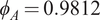 $ {\phi}_A=0.9812 $
) than their spouses (
$ {\phi}_A=0.9812 $
) than their spouses ( $ {\phi}_B=0.8898 $
). Spouses experience much more volatile, persistent income shocks and much less volatile transitory income shocks than household heads. The correlations between persistent earnings shocks and innovations to the return on the aggregate stock market turn out to be insignificant. The same holds for the correlation between the persistent earnings shocks experienced by household heads and spouses, consistent with results obtained by Blundell et al. (Reference Blundell, Pistaferri and Saporta-Eksten2016).
$ {\phi}_B=0.8898 $
). Spouses experience much more volatile, persistent income shocks and much less volatile transitory income shocks than household heads. The correlations between persistent earnings shocks and innovations to the return on the aggregate stock market turn out to be insignificant. The same holds for the correlation between the persistent earnings shocks experienced by household heads and spouses, consistent with results obtained by Blundell et al. (Reference Blundell, Pistaferri and Saporta-Eksten2016).
B. Calibration Choices for Dual-Income Households
In the baseline calibration, we set the risk aversion of both partners, $ A $
and
$ A $
and $ B $
, of the dual-income household to
$ B $
, of the dual-income household to $ {\gamma}_A={\gamma}_B=5 $
. Later, we will allow mean-preserving spreads in risk preferences and vary
$ {\gamma}_A={\gamma}_B=5 $
. Later, we will allow mean-preserving spreads in risk preferences and vary $ {\gamma}_A $
(
$ {\gamma}_A $
( $ {\gamma}_B $
) between 2 and 4 (8 and 6). This variation is motivated by Brooks et al. (Reference Brooks, Sangiorgi, Hillenbrand and Money2019) who find that men, on average, are more financially risk-tolerant than women, controlling for differences in age and employment status. The subjective discount factor is set to
$ {\gamma}_B $
) between 2 and 4 (8 and 6). This variation is motivated by Brooks et al. (Reference Brooks, Sangiorgi, Hillenbrand and Money2019) who find that men, on average, are more financially risk-tolerant than women, controlling for differences in age and employment status. The subjective discount factor is set to $ \beta =0.96 $
. The Pareto weight is assumed to be
$ \beta =0.96 $
. The Pareto weight is assumed to be $ \pi =0.5 $
in the baseline specification. Later, we will consider cases with
$ \pi =0.5 $
in the baseline specification. Later, we will consider cases with $ \pi =0.25 $
and
$ \pi =0.25 $
and $ \pi =0.75 $
.
$ \pi =0.75 $
.
The parameters of the earnings process are based on Table 1. Following Deaton (Reference Deaton1991), we assume that the estimated volatility parameters of the earnings process reflect, to some extent, measurement error. Correspondingly, we first reduce all estimated volatilities in Panel B of Table 1 by 50% for the baseline simulations. We then use the unadjusted estimated volatilities to investigate the saving and portfolio choice implications of a high-background-risk scenario. After age 65, we use $ 0.68 $
as the replacement ratio of retirement income to the last year’s income of working life. The maximum adult age is
$ 0.68 $
as the replacement ratio of retirement income to the last year’s income of working life. The maximum adult age is $ T=85 $
, corresponding to age 109.
$ T=85 $
, corresponding to age 109.
There are two financial assets, one risk-free asset (cash) and one risky asset (stocks). In line with Cocco et al. (Reference Cocco, Gomes and Maenhout2005), the risk-free asset yields a constant real gross return, $ {r}^f $
, of
$ {r}^f $
, of $ 2\% $
, while the mean equity premium,
$ 2\% $
, while the mean equity premium, $ \mu $
, is
$ \mu $
, is $ 4\% $
. The unconditional volatility of stock returns is
$ 4\% $
. The unconditional volatility of stock returns is $ 18\% $
.
$ 18\% $
.
IV. Simulation Results for Dual-Income Couples
There is a complication relative to unitary models when solving for optimal consumption. In collective models, the optimal division of total consumption between the two persons making up the household needs to be determined. Given a choice of total consumption, we use a bisection algorithm to solve for the optimal consumption share based on equation (10) for each cash-on-hand grid point and each age over the life cycle (see Appendix B for details). After solving for the policy functions (consumption of each partner and joint portfolio choice), we start the simulations across all experiments with all households having zero initial wealth for simplicity. We simulate 50,000 labor income shocks and calculate different moments of the optimal life-cycle profiles of wealth, individual consumption, and the share of wealth allocated to stocks (see Appendix C for details). Throughout Section IV, the collective model is solved for various combinations of risk preference and bargaining power parameters and compared to unitary benchmark models.
We first consider a unitary benchmark model for the collective model in which the representative agent has a coefficient of relative risk aversion that equals the arithmetic average of the coefficients of relative risk aversion of the two partners in the dual-income couple (Section IV.A). This setup allows us to investigate the impact of mean-preserving spreads in the partners’ coefficients of relative risk aversion on intra-household risk sharing and portfolio choice decisions (Section IV.B). Moreover, we compare the economic impact of the intra-household risk sharing and earnings risk-diversification channels on portfolio choice decisions (Section IV.C).
We then consider a unitary benchmark model in which the representative agent has a coefficient of relative risk aversion which equals the harmonic average of the coefficients of relative risk aversion of the two partners in the dual-income couple (Section IV.D). This setup allows us to evaluate whether the benchmark model can approximate the portfolio choice decisions in the collective model when partners with identical bargaining power differ in their risk preferences. We also investigate the accuracy of this approximation in a high-background-risk scenario resulting from a mean-preserving spread in idiosyncratic earnings risk (Section IV.E).
Finally, we introduce stock market participation costs to endogenously determine stock market participation in the model. This setup allows us to investigate the impact of mean-preserving spreads in the partners’ coefficients of relative risk aversion on stock market participation decisions (Section IV.F).
A. Partners with Identical Relative Risk Aversion
Figure 2 shows average simulated life-cycle profiles for a unitary benchmark model with $ \gamma =5 $
and three collective models with
$ \gamma =5 $
and three collective models with $ {\gamma}_A={\gamma}_B=5 $
and
$ {\gamma}_A={\gamma}_B=5 $
and $ \pi =\mathrm{0.25,0.50,0.75} $
, respectively. The representative agent in the unitary model receives the same earnings as the dual-income couple in the collective model. Graph A of Figure 2 shows the age profile of financial wealth, Graph B shows the profile of consumption, Graph C shows the profile of the share of wealth allocated to stocks, Graph D shows the profile of the couple’s relative risk aversion according to equation (12), and Graphs E and F show the profiles of the consumption shares for partners
$ \pi =\mathrm{0.25,0.50,0.75} $
, respectively. The representative agent in the unitary model receives the same earnings as the dual-income couple in the collective model. Graph A of Figure 2 shows the age profile of financial wealth, Graph B shows the profile of consumption, Graph C shows the profile of the share of wealth allocated to stocks, Graph D shows the profile of the couple’s relative risk aversion according to equation (12), and Graphs E and F show the profiles of the consumption shares for partners $ A $
and
$ A $
and $ B $
, respectively.
$ B $
, respectively.
Figure 2 shows average simulated life-cycle profiles for financial wealth (in Graph A), consumption (Graph B), the share of wealth allocated to stocks (Graph C), the relative risk aversion of the couple (Graph D), the consumption shares of partners A and B (Graphs E and F), obtained from the unitary life-cycle model with $ \gamma =5 $
and three collective models with
$ \gamma =5 $
and three collective models with $ {\gamma}_A={\gamma}_B=5 $
and
$ {\gamma}_A={\gamma}_B=5 $
and $ \pi =\mathrm{0.25,0.50,0.75} $
, respectively.
$ \pi =\mathrm{0.25,0.50,0.75} $
, respectively.

Given that both partners now have identical discount factors and individual preferences of the CRRA type with identical curvature parameters, the ISHARA conditions are fulfilled under which the collective model without portfolio choice can be replicated by the unitary benchmark model for an agent representing the dual-income couple (Mazzocco (Reference Mazzocco2004)). Graphs A and B of Figure 2 show that the unitary model and the three collective models with different Pareto weights yield identical life-cycle profiles of financial wealth and consumption. Importantly, we show that the same result applies to the share of financial wealth in stocks in Graph C, which decreases with the relative importance of human capital to financial wealth over the working life (see Cocco et al. (Reference Cocco, Gomes and Maenhout2005)) and stays relatively flat during retirement when earnings are risk-free.
Varying the Pareto weight does not affect saving and financial risk-taking in the collective model, provided both partners have the same risk aversion. The Pareto weight does, however, affect the distribution of consumption across partners as shown in Graphs E and F of Figure 2: the partner with higher bargaining power optimally receives a larger share of consumption. For example, the partner $ B $
in Graph F receives about 55% of consumption if
$ B $
in Graph F receives about 55% of consumption if $ \pi =0.75 $
, but only 45% of consumption if
$ \pi =0.75 $
, but only 45% of consumption if $ \pi =0.25 $
. The consumption shares of both partners are equal if the Pareto weight is
$ \pi =0.25 $
. The consumption shares of both partners are equal if the Pareto weight is $ \pi =0.5 $
. Reflecting the couple’s constant relative risk aversion across the life cycle in Graph D, the partners’ consumption shares are age-invariant as well.
$ \pi =0.5 $
. Reflecting the couple’s constant relative risk aversion across the life cycle in Graph D, the partners’ consumption shares are age-invariant as well.
B. Mean-Preserving Spreads in Relative Risk Aversion
We now depart from the ISHARA conditions and investigate the optimal behavior of a dual-income couple consisting of partners with different risk preferences. Figure 3 shows average simulated life-cycle profiles comparable to those in Figure 2, but obtained from collective models with $ \pi =0.50 $
and four different combinations of risk aversion within the couple:
$ \pi =0.50 $
and four different combinations of risk aversion within the couple: $ \left({\gamma}_A=5,{\gamma}_B=5\right) $
,
$ \left({\gamma}_A=5,{\gamma}_B=5\right) $
, $ \left({\gamma}_A=4,{\gamma}_B=6\right) $
,
$ \left({\gamma}_A=4,{\gamma}_B=6\right) $
, $ \left({\gamma}_A=3,{\gamma}_B=7\right) $
, and
$ \left({\gamma}_A=3,{\gamma}_B=7\right) $
, and $ \left({\gamma}_A=2,{\gamma}_B=8\right) $
. Thus, we consider models with an increasing spread in the partners’ risk aversion around the same arithmetic average risk aversion across the two partners (
$ \left({\gamma}_A=2,{\gamma}_B=8\right) $
. Thus, we consider models with an increasing spread in the partners’ risk aversion around the same arithmetic average risk aversion across the two partners ( $ \overline{\gamma}=5 $
). Recall from Section IV.A that the collective model with
$ \overline{\gamma}=5 $
). Recall from Section IV.A that the collective model with $ \left({\gamma}_A=5,{\gamma}_B=5\right) $
is identical to the unitary benchmark model with
$ \left({\gamma}_A=5,{\gamma}_B=5\right) $
is identical to the unitary benchmark model with $ \gamma =5 $
.
$ \gamma =5 $
.
Figure 3 shows average simulated life-cycle profiles for financial wealth (in Graph A), consumption (Graph B), the share of wealth allocated to stocks (Graph C), the relative risk aversion of the couple (Graph D), the consumption shares of partners A and B (Graphs E and F), obtained from four collective life-cycle models with $ \left({\gamma}_A=5,{\gamma}_B=5\right) $
,
$ \left({\gamma}_A=5,{\gamma}_B=5\right) $
, $ \left({\gamma}_A=4,{\gamma}_B=6\right) $
,
$ \left({\gamma}_A=4,{\gamma}_B=6\right) $
, $ \left({\gamma}_A=3,{\gamma}_B=7\right) $
, and
$ \left({\gamma}_A=3,{\gamma}_B=7\right) $
, and $ \left({\gamma}_A=2,{\gamma}_B=8\right) $
, respectively. The partners have identical bargaining power in all models (
$ \left({\gamma}_A=2,{\gamma}_B=8\right) $
, respectively. The partners have identical bargaining power in all models ( $ \pi =0.5 $
).
$ \pi =0.5 $
).

Figure 3 reveals the main result from simulating the calibrated life-cycle model: the more heterogeneous the partners are in risk preferences (for a given mean of their coefficients of relative risk aversion), the more they benefit from risk sharing, as evidenced by increased average financial wealth during retirement (Graph A) and increased average consumption across the life cycle (Graph B). This simultaneous increase in wealth and consumption is achieved by optimally allocating larger shares of financial wealth to stocks (Graph C). Financial risk-taking increases with the potential to share risk, and this potential is increasing with the mean-preserving spread between the partners’ individual coefficients of relative risk aversion. While a couple with $ \left({\gamma}_A=4,{\gamma}_B=6\right) $
on average allocates 1.6 percentage points (2.3%) more financial wealth to stocks than a couple with
$ \left({\gamma}_A=4,{\gamma}_B=6\right) $
on average allocates 1.6 percentage points (2.3%) more financial wealth to stocks than a couple with $ \left({\gamma}_A=5,{\gamma}_B=5\right) $
across the life cycle, this difference increases to a substantial 17.3 percentage points (24.7%) for a couple with
$ \left({\gamma}_A=5,{\gamma}_B=5\right) $
across the life cycle, this difference increases to a substantial 17.3 percentage points (24.7%) for a couple with $ \left({\gamma}_A=2,{\gamma}_B=8\right) $
. The largest increase in financial risk-taking in the latter case is observed at age 60.
$ \left({\gamma}_A=2,{\gamma}_B=8\right) $
. The largest increase in financial risk-taking in the latter case is observed at age 60.
This increase in the share of wealth in stocks is reflected in the couple’s coefficient of relative risk aversion (Graph D), which falls below the partners’ average individual risk aversion coefficient if the partners have different risk preferences. The more heterogeneous the partners are in risk preferences (for a given mean), the more risk-tolerant the couple becomes. While the relative risk aversion of a couple with $ \left({\gamma}_A=4,{\gamma}_B=6\right) $
on average falls below the relative risk aversion of a couple with
$ \left({\gamma}_A=4,{\gamma}_B=6\right) $
on average falls below the relative risk aversion of a couple with $ \left({\gamma}_A=5,{\gamma}_B=5\right) $
by 0.22 units across the life cycle, this difference increases to 1.84 units for a couple with
$ \left({\gamma}_A=5,{\gamma}_B=5\right) $
by 0.22 units across the life cycle, this difference increases to 1.84 units for a couple with $ \left({\gamma}_A=2,{\gamma}_B=8\right) $
. Importantly, a unitary model with a constant coefficient of relative risk aversion below the average individual risk aversion of the two partners is unable to exactly replicate the consumption and portfolio choice decisions of the couple in the collective model. This is because the collective model implies a U-shaped age profile of the couple’s relative risk aversion (Graph D), while relative risk aversion is age-invariant in the unitary model. We will investigate in Section IV.D, whether a unitary benchmark model can at least approximate the solutions of the collective model.
$ \left({\gamma}_A=2,{\gamma}_B=8\right) $
. Importantly, a unitary model with a constant coefficient of relative risk aversion below the average individual risk aversion of the two partners is unable to exactly replicate the consumption and portfolio choice decisions of the couple in the collective model. This is because the collective model implies a U-shaped age profile of the couple’s relative risk aversion (Graph D), while relative risk aversion is age-invariant in the unitary model. We will investigate in Section IV.D, whether a unitary benchmark model can at least approximate the solutions of the collective model.
Graphs E and F shed more light on the intra-household consumption-sharing rule in the collective model.Footnote
13 In line with the discussion under equation (11), the average consumption share of the more risk-tolerant partner $ A $
increases with household consumption over the working life, while the average consumption share of the more risk-averse partner
$ A $
increases with household consumption over the working life, while the average consumption share of the more risk-averse partner $ B $
declines. The slopes of these graphs are steeper the more the partners differ in risk preferences for a given mean relative risk aversion coefficient. In the special case of
$ B $
declines. The slopes of these graphs are steeper the more the partners differ in risk preferences for a given mean relative risk aversion coefficient. In the special case of $ \left({\gamma}_A=5,{\gamma}_B=5\right) $
, the collective model becomes observationally identical to the unitary benchmark model with
$ \left({\gamma}_A=5,{\gamma}_B=5\right) $
, the collective model becomes observationally identical to the unitary benchmark model with $ \gamma =5 $
, and the consumption shares are constant again as in Figure 2.
$ \gamma =5 $
, and the consumption shares are constant again as in Figure 2.
Figure 4 shows average simulated age profiles comparable to those in Figure 3, but investigates combinations of different Pareto weights, $ \pi =\mathrm{0.25,0.75} $
, with sets of individual risk aversions,
$ \pi =\mathrm{0.25,0.75} $
, with sets of individual risk aversions, $ \left({\gamma}_A=3,{\gamma}_B=7\right) $
and
$ \left({\gamma}_A=3,{\gamma}_B=7\right) $
and $ \left({\gamma}_A=2,{\gamma}_B=8\right) $
. The benefits from intra-household risk sharing documented earlier in Figure 3 for
$ \left({\gamma}_A=2,{\gamma}_B=8\right) $
. The benefits from intra-household risk sharing documented earlier in Figure 3 for $ \pi =0.50 $
remain present. The more heterogeneous the partners are in risk preferences for a given mean relative risk aversion coefficient, the more they are able to increase average wealth in retirement (Graph A of Figure 4) and average consumption across the life cycle (Graph B). Risk-taking (Graph C) increases as well, but now reflects to a larger extent the relative risk aversion of the partner with larger bargaining power. The larger the Pareto weight reflecting the bargaining power of partner
$ \pi =0.50 $
remain present. The more heterogeneous the partners are in risk preferences for a given mean relative risk aversion coefficient, the more they are able to increase average wealth in retirement (Graph A of Figure 4) and average consumption across the life cycle (Graph B). Risk-taking (Graph C) increases as well, but now reflects to a larger extent the relative risk aversion of the partner with larger bargaining power. The larger the Pareto weight reflecting the bargaining power of partner $ B $
for a given combination of
$ B $
for a given combination of $ \left({\gamma}_A,{\gamma}_B\right) $
, the more the couple’s relative risk aversion (Graph D) resembles the risk aversion of the more risk-averse partner
$ \left({\gamma}_A,{\gamma}_B\right) $
, the more the couple’s relative risk aversion (Graph D) resembles the risk aversion of the more risk-averse partner $ B $
, and the lower the share of wealth in stocks. For a given combination of
$ B $
, and the lower the share of wealth in stocks. For a given combination of $ \left({\gamma}_A,{\gamma}_B\right) $
, the partner with more bargaining power on average receives a larger share of consumption early in life when household consumption is relatively low but a lower share of consumption later in life (Graphs E and F).
$ \left({\gamma}_A,{\gamma}_B\right) $
, the partner with more bargaining power on average receives a larger share of consumption early in life when household consumption is relatively low but a lower share of consumption later in life (Graphs E and F).
Figure 4 shows average simulated life-cycle profiles for financial wealth (in Graph A), consumption (Graph B), the share of wealth allocated to stocks (Graph C), the relative risk aversion of the couple (Graph D), the consumption shares of partners A and B (Graphs E and F), obtained from four collective life-cycle models with combinations of $ \left({\gamma}_A=3,{\gamma}_B=7\right) $
,
$ \left({\gamma}_A=3,{\gamma}_B=7\right) $
, $ \left({\gamma}_A=2,{\gamma}_B=8\right) $
, and
$ \left({\gamma}_A=2,{\gamma}_B=8\right) $
, and $ \pi =\mathrm{0.25,0.75} $
.
$ \pi =\mathrm{0.25,0.75} $
.

C. Intra-Household Risk Sharing Versus Risk Diversification
Our main results in Figure 3 revealed a perhaps surprisingly large economic impact of intra-household risk sharing on portfolio choice. To further evaluate the economic importance of risk sharing, we now compare the quantitative implications of risk sharing with those of earnings risk diversification. Specifically, we solve the collective models with $ \left({\gamma}_A=4,{\gamma}_B=6\right) $
and
$ \left({\gamma}_A=4,{\gamma}_B=6\right) $
and $ \left({\gamma}_A=3,{\gamma}_B=7\right) $
and equal bargaining power for two different coefficients of correlation between the persistent earnings shocks of both partners,
$ \left({\gamma}_A=3,{\gamma}_B=7\right) $
and equal bargaining power for two different coefficients of correlation between the persistent earnings shocks of both partners, $ \rho =0.1 $
and
$ \rho =0.1 $
and $ \rho =0.9 $
. The parameter
$ \rho =0.9 $
. The parameter $ \rho $
directly affects the partners’ ability to diversify idiosyncratic earnings risk within the household. The solutions with
$ \rho $
directly affects the partners’ ability to diversify idiosyncratic earnings risk within the household. The solutions with $ \rho =0.1 $
are already known from Figure 3, but are repeated here for ease of comparison. Moving from a collective benchmark model with
$ \rho =0.1 $
are already known from Figure 3, but are repeated here for ease of comparison. Moving from a collective benchmark model with $ \left({\gamma}_A=3,{\gamma}_B=7\right) $
and
$ \left({\gamma}_A=3,{\gamma}_B=7\right) $
and $ \rho =0.1 $
to a model with
$ \rho =0.1 $
to a model with $ \left({\gamma}_A=3,{\gamma}_B=7\right) $
and
$ \left({\gamma}_A=3,{\gamma}_B=7\right) $
and $ \rho =0.9 $
reduces the scope for risk diversification but leaves the risk-sharing channel unaffected. This change can be motivated by Shore (Reference Shore2010) who finds that couples are less able to diversify idiosyncratic earnings risk during expansions. Similarly, moving from the same collective benchmark model to a collective model with
$ \rho =0.9 $
reduces the scope for risk diversification but leaves the risk-sharing channel unaffected. This change can be motivated by Shore (Reference Shore2010) who finds that couples are less able to diversify idiosyncratic earnings risk during expansions. Similarly, moving from the same collective benchmark model to a collective model with $ \left({\gamma}_A=4,{\gamma}_B=6\right) $
and
$ \left({\gamma}_A=4,{\gamma}_B=6\right) $
and $ \rho =0.1 $
reduces the scope for intra-household risk sharing but leaves the risk-diversification channel unaffected.
$ \rho =0.1 $
reduces the scope for intra-household risk sharing but leaves the risk-diversification channel unaffected.
Figure 5 shows the resulting simulation results. Compared to the benchmark collective model with $ \left({\gamma}_A=3,{\gamma}_B=7\right) $
and
$ \left({\gamma}_A=3,{\gamma}_B=7\right) $
and $ \rho =0.1 $
, a collective model with the same risk preference parameters and
$ \rho =0.1 $
, a collective model with the same risk preference parameters and $ \rho =0.9 $
on average leads to a
$ \rho =0.9 $
on average leads to a $ 1.7 $
percentage point (
$ 1.7 $
percentage point ( $ 2.2\% $
) reduction in the share of wealth allocated to stocks (in Graph C) across the life cycle. A higher correlation in the earnings streams of the partners increases nondiversifiable background risk, which in turn reduces financial risk-taking. Consumption (Graph B) is decreased early in life to increase precautionary saving and financial wealth (Graph A). In terms of economic magnitude, however, these changes are moderate, given the substantial increase from
$ 2.2\% $
) reduction in the share of wealth allocated to stocks (in Graph C) across the life cycle. A higher correlation in the earnings streams of the partners increases nondiversifiable background risk, which in turn reduces financial risk-taking. Consumption (Graph B) is decreased early in life to increase precautionary saving and financial wealth (Graph A). In terms of economic magnitude, however, these changes are moderate, given the substantial increase from $ \rho =0.1 $
to
$ \rho =0.1 $
to $ \rho =0.9 $
. This can also be seen from the collective coefficient of relative risk aversion of the couple (Graph D), which hardly changes.
$ \rho =0.9 $
. This can also be seen from the collective coefficient of relative risk aversion of the couple (Graph D), which hardly changes.
Figure 5 shows average simulated life-cycle profiles for financial wealth (in Graph A), consumption (Graph B), the share of wealth allocated to stocks (Graph C), the relative risk aversion of the couple (Graph D), the consumption shares of partners A and B (Graphs E and F), obtained from four collective life-cycle models which differ in their potential to share risk $ \left({\gamma}_A=4,{\gamma}_B=6\right) $
versus
$ \left({\gamma}_A=4,{\gamma}_B=6\right) $
versus $ \left({\gamma}_A=3,{\gamma}_B=7\right) $
, or diversify risk within the household,
$ \left({\gamma}_A=3,{\gamma}_B=7\right) $
, or diversify risk within the household, $ \rho =0.1 $
versus
$ \rho =0.1 $
versus $ \rho =0.9 $
. The partners have identical bargaining power in all models (
$ \rho =0.9 $
. The partners have identical bargaining power in all models ( $ \pi =0.5 $
).
$ \pi =0.5 $
).

Compared to the benchmark collective model with $ \left({\gamma}_A=3,{\gamma}_B=7\right) $
and
$ \left({\gamma}_A=3,{\gamma}_B=7\right) $
and $ \rho =0.1 $
, a collective model with
$ \rho =0.1 $
, a collective model with $ \left({\gamma}_A=4,{\gamma}_B=6\right) $
and
$ \left({\gamma}_A=4,{\gamma}_B=6\right) $
and $ \rho =0.1 $
, on average, leads to a
$ \rho =0.1 $
, on average, leads to a $ 5.4 $
percentage point (
$ 5.4 $
percentage point ( $ 7.0\% $
) reduction in the share of wealth allocated to stocks (in Graph C of Figure 5) across the life cycle. Thus, a relatively modest reduction in intra-household risk preference heterogeneity (leaving the average relative risk aversion coefficient unchanged) has a large economic impact on risk sharing and the share of wealth invested in stocks. This is reflected in the wealth (Graph A) and consumption (Graph B) profiles, which show that substantially more financial wealth is accumulated if the couple is less able to benefit from risk sharing. The risk-sharing channel clearly dominates the risk-diversification channel in economic magnitude in Figure 5.
$ 7.0\% $
) reduction in the share of wealth allocated to stocks (in Graph C of Figure 5) across the life cycle. Thus, a relatively modest reduction in intra-household risk preference heterogeneity (leaving the average relative risk aversion coefficient unchanged) has a large economic impact on risk sharing and the share of wealth invested in stocks. This is reflected in the wealth (Graph A) and consumption (Graph B) profiles, which show that substantially more financial wealth is accumulated if the couple is less able to benefit from risk sharing. The risk-sharing channel clearly dominates the risk-diversification channel in economic magnitude in Figure 5.
We know from Figure 3 that a mean-preserving spread in the partners’ coefficients of relative risk aversion from $ \left({\gamma}_A=5,{\gamma}_B=5\right) $
to
$ \left({\gamma}_A=5,{\gamma}_B=5\right) $
to $ \left({\gamma}_A=4,{\gamma}_B=6\right) $
has less impact on savings and portfolio choice than an equally sized mean-preserving spread from
$ \left({\gamma}_A=4,{\gamma}_B=6\right) $
has less impact on savings and portfolio choice than an equally sized mean-preserving spread from $ \left({\gamma}_A=4,{\gamma}_B=6\right) $
to
$ \left({\gamma}_A=4,{\gamma}_B=6\right) $
to $ \left({\gamma}_A=3,{\gamma}_B=7\right) $
. In unreported results, we find that the risk-sharing and risk-diversification channels are similar in economic magnitude if Figure 5 is repeated for a benchmark collective model with
$ \left({\gamma}_A=3,{\gamma}_B=7\right) $
. In unreported results, we find that the risk-sharing and risk-diversification channels are similar in economic magnitude if Figure 5 is repeated for a benchmark collective model with $ \left({\gamma}_A=4,{\gamma}_B=6\right) $
and
$ \left({\gamma}_A=4,{\gamma}_B=6\right) $
and $ \rho =0.1 $
. This is still remarkable, considering that a modest change in the partners’ coefficients of relative risk aversion (leaving the average coefficient unchanged) is compared to a substantial change in the intra-household correlation of persistent idiosyncratic earnings shocks. In summary, the intra-household risk-sharing channel that affects all couples has larger portfolio choice implications than the risk-diversification channel that only affects dual-income couples.
$ \rho =0.1 $
. This is still remarkable, considering that a modest change in the partners’ coefficients of relative risk aversion (leaving the average coefficient unchanged) is compared to a substantial change in the intra-household correlation of persistent idiosyncratic earnings shocks. In summary, the intra-household risk-sharing channel that affects all couples has larger portfolio choice implications than the risk-diversification channel that only affects dual-income couples.
D. Can a Unitary Model Approximate the Collective Model?
As a benchmark for the analysis of mean-preserving spreads in the partners’ coefficients of relative risk aversion in the collective model, we use a unitary model with a coefficient of risk aversion equal to the arithmetic average risk aversion coefficient of the partners in Section IV.B. Compared to this benchmark, we show that mean-preserving spreads in risk aversion have large economic effects on financial risk-taking. We now investigate whether a different unitary benchmark model can approximate these results from the collective life-cycle portfolio choice model when partners differ in relative risk aversion.
We already know that the consumption and portfolio choice decisions of the collective model can be exactly replicated by a unitary model if the partners have identical risk preferences. We also know that it is impossible for a unitary model to replicate the results of the collective model if there is intra-household heterogeneity in risk preferences because, in this case, the couple’s collective risk aversion varies across the life cycle as a function of time-varying individual consumption shares. However, the U-shaped profile of the couple’s risk aversion coefficient across the life-cycle is not very pronounced in Figure 3, which raises the question whether we can find a unitary model with an age-invariant relative risk aversion coefficient that yields a good approximation to the collective model for a couple. This is an important question because the unitary model is the workhorse model in the life-cycle portfolio choice literature.
As already indicated in Section II.D, we propose using a unitary model with the coefficient of relative risk aversion in equation (13) as a benchmark for approximating the collective model. This coefficient replaces the age-varying individual consumption shares in the denominator of the true coefficient of risk aversion in the collective model in equation (12) with the bargaining power weights of the partners. Gu et al. (Reference Gu, Peng and Zhang2024) parameterize these bargaining weights as functions of observable variables such as the relative earnings of the partners. This variable can also be generated from an assumed earnings process for a dual-income couple such as ours in Section II.A. Thus, unlike individual consumption shares, these bargaining weights can be generated in the process of solving a unitary life-cycle portfolio choice model.
For the following simulations, we assume that partners have identical bargaining power. In this case, the coefficient of relative risk aversion in equation (13) becomes the harmonic mean of the partners’ coefficients of relative risk aversion. The harmonic mean also results from the collective model if the partners share consumption equally within the household (see equation (12)) as assumed by Love (Reference Love2010), Hong and Ríos-Rull (Reference Hong and Ríos-Rull2012), and Hubener et al. (Reference Hubener, Maurer and Mitchell2015). However, equal consumption sharing is usually not an outcome of the collective model if partners differ in risk preferences. If the partners have identical bargaining power, risk sharing in the collective model instead implies equal marginal utility of consumption.
Figure 6 shows simulation results from two collective models with intra-household heterogeneity in relative risk aversion, $ \left({\gamma}_A=3,{\gamma}_B=7\right) $
and
$ \left({\gamma}_A=3,{\gamma}_B=7\right) $
and $ \left({\gamma}_A=2,{\gamma}_B=8\right) $
. All other parameters are set to their calibration values. These results are already known from Figure 3, but are repeated here for ease of comparison. Also shown in Figure 6 are the results from two unitary models with coefficients of relative risk aversion equal to
$ \left({\gamma}_A=2,{\gamma}_B=8\right) $
. All other parameters are set to their calibration values. These results are already known from Figure 3, but are repeated here for ease of comparison. Also shown in Figure 6 are the results from two unitary models with coefficients of relative risk aversion equal to $ \gamma =4.2 $
(the harmonic mean of 3 and 7) and
$ \gamma =4.2 $
(the harmonic mean of 3 and 7) and $ \gamma =3.2 $
(the harmonic mean of 2 and 8), respectively. For the unitary models, we plot consumption shares of 0.5 in Graphs E and F of Figure 6 in line with assuming identical bargaining power. We deliberately choose collective models with relatively large differences in individual risk aversion, which lead to relatively pronounced U-shaped life-cycle profiles in the couple’s relative risk aversion, as can be seen from Figure 3. If the unitary benchmark model serves as a good approximation to these models, it will do even better when there is less heterogeneity in risk aversion.
$ \gamma =3.2 $
(the harmonic mean of 2 and 8), respectively. For the unitary models, we plot consumption shares of 0.5 in Graphs E and F of Figure 6 in line with assuming identical bargaining power. We deliberately choose collective models with relatively large differences in individual risk aversion, which lead to relatively pronounced U-shaped life-cycle profiles in the couple’s relative risk aversion, as can be seen from Figure 3. If the unitary benchmark model serves as a good approximation to these models, it will do even better when there is less heterogeneity in risk aversion.
Figure 6 shows average simulated life-cycle profiles for financial wealth (in Graph A), consumption (Graph B), the share of wealth allocated to stocks (Graph C), the relative risk aversion of the couple (Graph D), the consumption shares of partners A and B (Graphs E and F), obtained from two collective life-cycle models with $ \left({\gamma}_A=3,{\gamma}_B=7\right) $
and
$ \left({\gamma}_A=3,{\gamma}_B=7\right) $
and $ \left({\gamma}_A=2,{\gamma}_B=8\right) $
and two unitary models with
$ \left({\gamma}_A=2,{\gamma}_B=8\right) $
and two unitary models with $ \gamma =4.2 $
(the harmonic mean of 3 and 7) and
$ \gamma =4.2 $
(the harmonic mean of 3 and 7) and $ \gamma =3.2 $
(the harmonic mean of 2 and 8), respectively. The partners have identical bargaining power in all models (
$ \gamma =3.2 $
(the harmonic mean of 2 and 8), respectively. The partners have identical bargaining power in all models ( $ \pi =0.5 $
).
$ \pi =0.5 $
).

In terms of portfolio choice (see Graph C of Figure 6), the unitary models provide very good approximations to the collective models. The difference in the average risky asset share across the life cycle is about 0.3 percentage points for $ \left({\gamma}_A=3,{\gamma}_B=7\right) $
and 1.1 percentage points for
$ \left({\gamma}_A=3,{\gamma}_B=7\right) $
and 1.1 percentage points for $ \left({\gamma}_A=2,{\gamma}_B=8\right) $
. However, compared to the unitary benchmark model, the couple in the collective model enjoys higher average consumption across the life cycle (Graph B). Compared to the unitary model with
$ \left({\gamma}_A=2,{\gamma}_B=8\right) $
. However, compared to the unitary benchmark model, the couple in the collective model enjoys higher average consumption across the life cycle (Graph B). Compared to the unitary model with $ \gamma =4.2 $
(
$ \gamma =4.2 $
( $ \gamma =3.2 $
), the collective model with
$ \gamma =3.2 $
), the collective model with $ \left({\gamma}_A=3,{\gamma}_B=7\right) $
(
$ \left({\gamma}_A=3,{\gamma}_B=7\right) $
( $ \left({\gamma}_A=2,{\gamma}_B=8\right) $
) increases average household consumption by
$ \left({\gamma}_A=2,{\gamma}_B=8\right) $
) increases average household consumption by $ 1.0\% $
(
$ 1.0\% $
( $ 2.4\% $
). The largest increase occurs during retirement. The consumption loss experienced by the couple in the unitary model with a harmonic average risk aversion coefficient can be interpreted as the loss resulting from sharing consumption equally as opposed to sharing consumption optimally. This interpretation is based on the collective coefficient of relative risk aversion in equation (12), which reduces to the harmonic mean of the partners’ coefficients of relative risk aversion if consumption is shared equally.
$ 2.4\% $
). The largest increase occurs during retirement. The consumption loss experienced by the couple in the unitary model with a harmonic average risk aversion coefficient can be interpreted as the loss resulting from sharing consumption equally as opposed to sharing consumption optimally. This interpretation is based on the collective coefficient of relative risk aversion in equation (12), which reduces to the harmonic mean of the partners’ coefficients of relative risk aversion if consumption is shared equally.
The unitary benchmark model in this analysis approximates the risk-sharing mechanism of the collective model. It is therefore interesting to see the differences between the two models if background risk increases. For this purpose, we repeat the simulations underlying Figure 6 with an earnings process that employs the full magnitude of the estimated volatilities in Panel B of Table 1.Footnote 14 Recall that we reduced these volatilities for our previous simulations by 50% to account for possible measurement error. We discuss the results of these simulations in Figure 7 in Section IV.E.
Figure 7 replicates Figure 6 for a high-earnings-risk scenario. The figure shows average simulated life-cycle profiles for financial wealth (in Graph A), consumption (Graph B), the share of wealth allocated to stocks (Graph C), the relative risk aversion of the couple (Graph D), the consumption shares of partners A and B (Graphs E and F), obtained from two collective life-cycle models with $ \left({\gamma}_A=3,{\gamma}_B=7\right) $
and
$ \left({\gamma}_A=3,{\gamma}_B=7\right) $
and $ \left({\gamma}_A=2,{\gamma}_B=8\right) $
and two unitary models with
$ \left({\gamma}_A=2,{\gamma}_B=8\right) $
and two unitary models with $ \gamma =4.2 $
(the harmonic mean of 3 and 7) and
$ \gamma =4.2 $
(the harmonic mean of 3 and 7) and $ \gamma =3.2 $
(the harmonic mean of 2 and 8), respectively. The partners have identical bargaining power in all models (
$ \gamma =3.2 $
(the harmonic mean of 2 and 8), respectively. The partners have identical bargaining power in all models ( $ \pi =0.5 $
).
$ \pi =0.5 $
).

E. Mean-Preserving Spreads in Idiosyncratic Earnings Risk
Before we compare the unitary and collective models in Figure 7, we note the substantial increase in financial wealth in Figure 7 (Graph A) compared to Figure 6 (Graph A). This is due to higher precautionary savings in response to increased background risk. This result is expected because the individual power utility in our model is characterized by prudence. Apps et al. (Reference Apps, Andrienko and Rees2014) show that precautionary saving increases in the collective model in response to a mean-preserving spread in earnings risk if individual preferences exhibit prudence, in line with the unitary case considered by Kimball (Reference Kimball1990). Compared to the couple with $ \left({\gamma}_A=3,{\gamma}_B=7\right) $
, the couple with
$ \left({\gamma}_A=3,{\gamma}_B=7\right) $
, the couple with $ \left({\gamma}_A=2,{\gamma}_B=8\right) $
accumulates less precautionary savings in response to the mean-preserving spread in earnings risk, reflecting the larger potential to share risk within the household.
$ \left({\gamma}_A=2,{\gamma}_B=8\right) $
accumulates less precautionary savings in response to the mean-preserving spread in earnings risk, reflecting the larger potential to share risk within the household.
The increase in precautionary savings is accompanied by a substantial reduction in the share of wealth in stocks (see Graph C of Figures 6 and 7). Higher background risk crowds out financial risk-taking. The mean-preserving spread in earnings risk reduces the average risky asset share across the life cycle from $ 77\% $
to
$ 77\% $
to $ 67\% $
for
$ 67\% $
for $ \left({\gamma}_A=3,{\gamma}_B=7\right) $
and from
$ \left({\gamma}_A=3,{\gamma}_B=7\right) $
and from $ 87\% $
to
$ 87\% $
to $ 78\% $
for
$ 78\% $
for $ \left({\gamma}_A=2,{\gamma}_B=8\right) $
.Footnote
15
$ \left({\gamma}_A=2,{\gamma}_B=8\right) $
.Footnote
15
In this environment with increased background risk, the unitary models with harmonic average risk aversion coefficients provide worse approximations to the consumption and portfolio choice decisions in the collective models. While the average difference in the risky asset shares between unitary and collective models remains small over the life cycle (0.6 and 1.2 percentage points, respectively, for the collective models with $ \left({\gamma}_A=3,{\gamma}_B=7\right) $
and
$ \left({\gamma}_A=3,{\gamma}_B=7\right) $
and $ \left({\gamma}_A=2,{\gamma}_B=8\right) $
), there are now substantial timing differences, with the collective models generating smaller (larger) allocations to risky assets during working life (retirement) than the unitary models. For example, the average share of wealth in risky assets at age 60 is
$ \left({\gamma}_A=2,{\gamma}_B=8\right) $
), there are now substantial timing differences, with the collective models generating smaller (larger) allocations to risky assets during working life (retirement) than the unitary models. For example, the average share of wealth in risky assets at age 60 is $ 65\% $
for the collective model with
$ 65\% $
for the collective model with $ \left({\gamma}_A=2,{\gamma}_B=8\right) $
, but
$ \left({\gamma}_A=2,{\gamma}_B=8\right) $
, but $ 72\% $
for the unitary model with
$ 72\% $
for the unitary model with $ \gamma =3.2 $
.
$ \gamma =3.2 $
.
This is due to an increase in the consumption share of the more risk-averse partner B early in life (when consumption closely follows income) in response to high earnings volatility, which increases the couple’s relative risk aversion (see equation (12)) and decreases the share of wealth in stocks relative to the unitary model. When more wealth is accumulated later in life, negative earnings shocks no longer affect household consumption to the same extent, and the share of consumption of the less risk-averse partner A increases. Correspondingly, the couple’s relative risk aversion decreases, and the share of wealth in stocks increases relative to the unitary model.
Moreover, the differences in average consumption between unitary and collective models are even more pronounced when background risk increases. Compared to the unitary model with $ \gamma =4.2 $
(
$ \gamma =4.2 $
( $ \gamma =3.2 $
), the collective model with
$ \gamma =3.2 $
), the collective model with $ \left({\gamma}_A=3,{\gamma}_B=7\right) $
(
$ \left({\gamma}_A=3,{\gamma}_B=7\right) $
( $ \left({\gamma}_A=3,{\gamma}_B=7\right) $
) increases average household consumption by
$ \left({\gamma}_A=3,{\gamma}_B=7\right) $
) increases average household consumption by $ 1.4\% $
(
$ 1.4\% $
( $ 3.5\% $
). The largest increase again occurs during retirement.
$ 3.5\% $
). The largest increase again occurs during retirement.
In summary, while a unitary model with a relative risk aversion coefficient in equation (13) can approximate the average share of wealth in stocks across the life cycle generated by a collective model with a relative risk aversion coefficient in equation (12), the unitary model has problems in replicating the timing of portfolio choice decisions across the life cycle if background risk is high. Moreover, the unitary model generates less household consumption than the collective model, in particular during retirement.
When is background risk high? In our case, the high-background-risk scenario results from taking literally the GMM estimates of the covariance parameters of the couple’s joint earnings process. The low-background-risk scenario attributes half of the estimated volatilities of the earnings process to measurement error. Thus, it is safe to assume that the unitary model will have problems in replicating the consumption and portfolio choice decisions of the collective model if earnings process parameters are not adjusted for measurement error, as in Deaton (Reference Deaton1991).
F. Stock Market Participation
In the absence of stock market participation costs, all households in our model optimally hold stocks. As a robustness check, we now add stock market participation costs to the model in line with Vissing-Jorgensen (Reference Vissing-Jorgensen2002), Gomes and Michaelides (Reference Gomes and Michaelides2005), Fagereng, Gottlieb, and Guiso (Reference Fagereng, Gottlieb and Guiso2017), Gu et al. (Reference Gu, Peng and Zhang2024) and others. To this end, we assume that a percentage $ F $
of the household’s earnings is paid as a nonrecurring fee when the household decides to enter the stock market for the first time. These costs may reflect pecuniary and nonpecuniary components related to setting up a trading account and learning how to trade. Afterward, a percentage
$ F $
of the household’s earnings is paid as a nonrecurring fee when the household decides to enter the stock market for the first time. These costs may reflect pecuniary and nonpecuniary components related to setting up a trading account and learning how to trade. Afterward, a percentage $ f $
of the household’s earnings is paid out as recurring fees each period, as long as the household remains invested in the stock market.
$ f $
of the household’s earnings is paid out as recurring fees each period, as long as the household remains invested in the stock market.
Figure 8 shows simulation results from two collective models with intra-household heterogeneity in relative risk aversion, $ \left({\gamma}_A=4,{\gamma}_B=6\right) $
and
$ \left({\gamma}_A=4,{\gamma}_B=6\right) $
and $ \left({\gamma}_A=2,{\gamma}_B=8\right) $
. Both models are solved for
$ \left({\gamma}_A=2,{\gamma}_B=8\right) $
. Both models are solved for $ F=5\% $
initial stock market participation costs and either
$ F=5\% $
initial stock market participation costs and either $ f=2\% $
or
$ f=2\% $
or $ f=1\% $
repeated stock market participation costs.Footnote
16 All other parameters are set to their calibration values. The choice of collective models is guided by the simulation results of Section IV.E, which establishes a higher precautionary savings motive for households that are less able to share risk within the household (
$ f=1\% $
repeated stock market participation costs.Footnote
16 All other parameters are set to their calibration values. The choice of collective models is guided by the simulation results of Section IV.E, which establishes a higher precautionary savings motive for households that are less able to share risk within the household ( $ \left({\gamma}_A=4,{\gamma}_B=6\right) $
relative to
$ \left({\gamma}_A=4,{\gamma}_B=6\right) $
relative to $ \left({\gamma}_A=2,{\gamma}_B=8\right) $
). Thus, the savings motive decreases with a mean-preserving spread in the partners’ individual risk aversion coefficients.
$ \left({\gamma}_A=2,{\gamma}_B=8\right) $
). Thus, the savings motive decreases with a mean-preserving spread in the partners’ individual risk aversion coefficients.
Figure 8 shows average simulated life-cycle profiles for financial wealth (in Graph A), consumption (Graph B), the share of wealth allocated to stocks (Graph C), the relative risk aversion of the couple (Graph D), the consumption share of partner A (Graph E), and stock market participation (Graph F), obtained from two collective life-cycle models with $ \left({\gamma}_A=4,{\gamma}_B=6\right) $
and
$ \left({\gamma}_A=4,{\gamma}_B=6\right) $
and $ \left({\gamma}_A=2,{\gamma}_B=8\right) $
, respectively, and two combinations of initial (
$ \left({\gamma}_A=2,{\gamma}_B=8\right) $
, respectively, and two combinations of initial ( $ F $
) and recurring (
$ F $
) and recurring ( $ f $
) stock market participation costs, (
$ f $
) stock market participation costs, ( $ F=5\%,f=2\% $
) and (
$ F=5\%,f=2\% $
) and ( $ F=5\%,f=1\% $
). Graphs A–E refer to stockholders only. The partners have identical bargaining power in all models (
$ F=5\%,f=1\% $
). Graphs A–E refer to stockholders only. The partners have identical bargaining power in all models ( $ \pi =0.5 $
).
$ \pi =0.5 $
).

Figure 8 is organized along the lines of previous figures. However, Graph F now shows the percentage of stockholders across the life cycle instead of the consumption share of the partner $ B $
(which still can be recovered as 1 minus the consumption share of the partner
$ B $
(which still can be recovered as 1 minus the consumption share of the partner $ A $
in Graph E). The average stock market participation across the life cycle has a hump-shaped pattern. Early in life, some liquidity-constrained households optimally decide to stay out of the stock market. By age 40, almost all households participate in the stock market, regardless of risk preferences and the magnitude of stock market participation fees. Households remain invested in the stock market until late in life.
$ A $
in Graph E). The average stock market participation across the life cycle has a hump-shaped pattern. Early in life, some liquidity-constrained households optimally decide to stay out of the stock market. By age 40, almost all households participate in the stock market, regardless of risk preferences and the magnitude of stock market participation fees. Households remain invested in the stock market until late in life.
We find that a mean-preserving spread in the partners’ individual risk aversion coefficients decreases average stock market participation early in life. With recurring participation fees set to $ f=2\% $
(
$ f=2\% $
( $ f=1\% $
), 65.5% (74.6%) of couples aged 40 and under with
$ f=1\% $
), 65.5% (74.6%) of couples aged 40 and under with $ \left({\gamma}_A=4,{\gamma}_B=6\right) $
participate in the stock market, while only 63.6% (73.8%) of couples with
$ \left({\gamma}_A=4,{\gamma}_B=6\right) $
participate in the stock market, while only 63.6% (73.8%) of couples with $ \left({\gamma}_A=2,{\gamma}_B=8\right) $
optimally decide to invest in stocks. This result is consistent with the reduced savings motive of couples that have better opportunities to share risk within the household.
$ \left({\gamma}_A=2,{\gamma}_B=8\right) $
optimally decide to invest in stocks. This result is consistent with the reduced savings motive of couples that have better opportunities to share risk within the household.
Conditional on participation, the share of wealth in stocks (in Graph C of Figure 8) increases with a mean-preserving spread in relative risk aversion, confirming our earlier simulation results in Section IV.B. There are some differences at the end of life as stock market participation begins to drop, and the consumption share of partner A now rises at the end of life. This happens due to a selection effect; it is costly to participate in the stock market, and we are reporting the households that continue to participate. They tend to be wealthier than those who drop out, and therefore have higher consumption (Graph B). For these households, higher total consumption implies a higher consumption share for the less risk-averse partner (Graph E).
We emphasize that the opposite effects of a mean-preserving spread in relative risk aversion on stock market participation (negative impact) and the share of wealth in stocks conditional on participation (positive impact) do not contradict each other. Intra-household risk sharing reduces precautionary savings. Only households with a sufficient savings motive are willing to bear the participation costs. Thus, participation decreases with a mean-preserving spread in relative risk aversion. However, conditional on participation, the share of wealth in stocks increases with the potential to share risk within the household. Thus, financial risk-taking increases with a mean-preserving spread in relative risk aversion, conditional on participation.
V. Supportive Empirical Evidence
Our simulations of the collective life-cycle portfolio choice model have clear implications for any empirical analysis of financial risk-taking at the household level. For couples, variables describing the potential to share risk within the household should be among the set of characteristics explaining stock market participation and the share of wealth allocated to stocks, conditional on participation. Our analysis focuses on intra-household differences in relative risk aversion as the key driver of risk sharing. Controlling for the average coefficient of risk aversion within the household, the difference in the partner’s coefficients of relative risk aversion becomes a key explanatory variable explaining the financial risk-taking of couples.
If such information is not available in the data, proxies can be used. For example, ownership of life and long-term care insurance is positively related to the willingness to take financial risks (Eling, Ghavibazoo, and Hanewald (Reference Eling, Ghavibazoo and Hanewald2021)). Correspondingly, interactions of dummy variables indicating insurance ownership of the partners could be used to capture differences in their risk aversion coefficients.
In this section, we provide an empirical analysis of financial risk-taking using data from the HILDA Survey, which contains information on the individual risk aversion of both partners within a couple. If the collective portfolio choice model describes the actual behavior of households, then we should find a positive and significant impact of the absolute value of the difference in partners’ relative risk aversion on the share of wealth allocated to the stock market, conditional on participation.
A. Household Data
While we use U.S. data to calibrate our model, we use data from the Household, Income and Labour Dynamics in Australia (HILDA) Survey in this section to investigate the relationship between the financial risk-taking of couples and intra-household heterogeneity in risk aversion. Based on a comparison of several U.S. and international data sets, Gu et al. (Reference Gu, Peng and Zhang2024) conclude that HILDA is the most suitable data source for analyzing intra-household financial decisions. HILDA is a nationally representative, annual panel of Australian households, which commenced in 2001.Footnote 17 For our purposes, the main advantage of HILDA compared to other data sets is the availability of a measure of individual risk aversion for both partners in couples over the full working life.
Information on financial wealth and portfolio choice is collected every 4 years in HILDA as part of the wealth module. We use the six waves of HILDA between 2002 and 2022 that include a wealth module for our analysis. We create an unbalanced panel of couples consisting of partners aged 25–65 whose individual risk aversion can be assessed (see below). There are 6,158 couples in our final sample with 14,029 couple-year observations. Thus, on average, each couple is observed for about 9 years (2.3 periods). The subsample of households holding stocks (stockholders, from now on) consists of 6,494 couple-year observations and includes 3,154 couples.
Individual risk aversion in HILDA is equal to the value 1 (2) [3] if a respondent reports a willingness to take substantial (above-average) [average] financial risks with their spare cash, and the value 4 if the respondent is not willing to take any financial risks. In line with Gu et al. (Reference Gu, Peng and Zhang2024), we remove missing values and exclude couples in which at least one partner responds with “never has any spare cash” (value 5).Footnote 18
Following Gu et al. (Reference Gu, Peng and Zhang2024), we first interpret the ordinal measure of individual risk aversion as if it were a cardinal measure. As a robustness check, we then create a cardinal measure of individual risk aversion based on a transformation of the ordinal variable proposed by Winship and Mare (Reference Winship and Mare1984) and Terza (Reference Terza1987).Footnote 19 This transformation has been applied in previous literature to create, for example, cardinal measures of bond ratings (Wu (Reference Wu1993)) and risk aversion (Botzen and van den Bergh (Reference Botzen and van den Bergh2012)). Based on these measures of individual risk aversion, we calculate the “Difference in risk aversion” as the absolute value of the difference in the partners’ individual risk aversion measures. We define “Average risk aversion” as the arithmetic average of the partners’ measures of individual risk aversion.
Table 2 shows summary statistics for all couples (in Panel A), and stockholders (Panel B). Forty-six percent of households hold stocks, either directly or indirectly through mutual funds. Financial wealth includes bank accounts, cash and bond holdings, direct and indirect stockholdings, trusts, and the cash value of life insurance. Based on this, we create a “Log financial wealth” variable. The “Share of wealth in stocks,” defined as the share of financial wealth in direct or indirect stockholdings, is the variable of interest for the following analysis. Conditional on participation in the stock market, the average share of financial wealth in stocks is 43%.

Among stockholders, we find an average difference in the ordinal (cardinal) measure of risk aversion of 0.54 (0.75) in the sample (Panel B in Table 2). In 47.2% of these couples, the difference in risk aversion is positive. Including nonstockholders, this number decreases to 45.5% (Panel A). Gu et al. (Reference Gu, Peng and Zhang2024) report a slightly lower percentage of 43.4% using the 2006–2018 waves of HILDA with the wealth module only, while Mazzocco (Reference Mazzocco2004) finds a slightly higher percentage of 48.2% among elderly couples in the HRS. In any case, almost half of couples are not perfectly matched in terms of risk preferences. The average ordinal measure of risk aversion among stockholders is 3.1. As expected, this average is higher (3.25) for the whole sample.
Finally, we construct “Average age/10” and “Average age squared/100” variables that refer to the average age of partners in couples, scaled by 10. These variables are meant to pick up life-cycle patterns in financial risk-taking. The average age in our sample of couples with partners aged 25–65 is 44.3 (Panel A in Table 2). Stockholders, on average, are slightly older (46.1, Panel B) than nonstockholders.
B. Empirical Analysis
Using multivariate regression analysis, we investigate the relationship between the financial risk-taking of couples at the extensive and intensive margin and the ability of couples to share risk within the household. In line with our simulation results in Section IV, we focus on the difference in the partners’ coefficients of relative risk aversion as the main explanatory variable, while controlling for the average risk aversion.
Following Campbell (Reference Campbell2006), we separate the decision to participate in the stock market from the share of wealth invested in the stock market, conditional on participation. This share of wealth equals 100% for around 0.82% of couple-year observations. Correspondingly, we use a right-censored regression model (pooled Tobit) for the analysis of the intensive margin of risk-taking. For the analysis of the extensive margin, we use a pooled Probit model. By construction, we need to use linear regression models for both analyses if the key explanatory variables are based on the cardinal measure of individual risk aversion.
Table 3 shows the estimation results for the extensive and intensive margins of financial risk-taking and the three measures of risk aversion. The key explanatory variables in Panel A and Panel B of Table 3 are based on the ordinal and cardinal measures of individual risk aversion, respectively. All regressions include a full set of (unreported) time dummy variables. We present estimated, average partial effects (APEs) for all nonlinear models, which are comparable to the estimated coefficients in the linear models. The estimated standard errors are clustered at the household level to allow for within-couple serial correlation in error terms caused, for example, by unobserved, time-invariant, heterogeneity.

In line with most of our simulation results in Section IV, which abstract from the stock market participation decision except in Section IV.F, we first discuss the results for the share of wealth invested in stocks, conditional on participation. Importantly, the APE for the intra-household “Difference in risk aversion” is positive and statistically significant at the 5% level in all regressions, irrespective of the method of construction of the measure of individual risk aversion. For the ordinal and cardinal measures in Panels A and B of Table 3, a one-unit increase in the difference in individual risk preferences increases the share of wealth in stocks by 1.3 percentage points.
For comparison, our simulation results in Graph C of Figure 3 show that a couple consisting of partners with individual risk aversion coefficients of 4 and 6, respectively, on average allocates 1.1 percentage points more financial wealth to stocks over their working life than a couple consisting of partners with identical risk aversion coefficients of 5. For larger mean-preserving spreads, we find more substantial increases. Thus, we find empirical support for the predicted positive relationship between mean-preserving spreads in risk aversion and financial risk-taking at the intensive margin. Quantitatively, the empirical findings are in the vicinity of model predictions.
An increase in the intra-household “Average risk aversion” has the predicted negative impact on financial risk-taking. A one-unit increase in average individual risk aversion decreases the share of wealth in stocks by more than 10 (8) percentage points in Panel A (B) of Table 3. The APE is statistically significant at the 1% level. This result gives us confidence that our measures of individual risk aversion indeed capture the risk preferences of the partners. In addition, we find a hump-shaped age pattern in the share of wealth allocated to stocks in both panels of Table 3. However, the age effects are statistically insignificant. The APE of “Log financial wealth” is negative but insignificant in both panels.
We next discuss the results for the stock market participation decision, which we investigated in the simulations in Section IV.F. The $ {R}^2 $
of the linear probability model for the extensive margin of financial risk-taking, 0.27 (in Panel B of Table 3), substantially exceeds the corresponding statistic of the linear model for the intensive margin, 0.07. Thus, it is less difficult to explain variation in stock market participation than variation in the demand for stocks, conditional on participation.
$ {R}^2 $
of the linear probability model for the extensive margin of financial risk-taking, 0.27 (in Panel B of Table 3), substantially exceeds the corresponding statistic of the linear model for the intensive margin, 0.07. Thus, it is less difficult to explain variation in stock market participation than variation in the demand for stocks, conditional on participation.
Contrary to our findings at the intensive margin, the intra-household difference in risk aversion usually has a negative impact on the extensive margin of financial risk-taking. A one-unit increase in the difference in individual risk preferences decreases stock market participation by 1.6 (1.1) percentage points for the ordinal (cardinal) measure of individual risk aversion in Panel A (Panel B) of Table 3. These effects are statistically significant at the 5% level. Recall that we find a 1.9% (0.8%) reduction in the stock market participation of couples aged 40 and under with $ \left({\gamma}_A=2,{\gamma}_B=8\right) $
compared to those with
$ \left({\gamma}_A=2,{\gamma}_B=8\right) $
compared to those with $ \left({\gamma}_A=4,{\gamma}_B=6\right) $
in Section IV.F for participation fees
$ \left({\gamma}_A=4,{\gamma}_B=6\right) $
in Section IV.F for participation fees $ f=2\% $
(
$ f=2\% $
( $ f=1\% $
). Thus, our empirical results resemble those generated from the simulations of our model.
$ f=1\% $
). Thus, our empirical results resemble those generated from the simulations of our model.
There are at least two explanations for this finding: participation costs and intra-household cooperation. The first explanation is directly related to the model. Only households with a sufficiently strong savings motive are willing to bear the costs of stock market participation. The savings motive is higher for couples who are less able to share risk within the household, as shown in Section IV.E. Thus, a mean-preserving spread in relative risk aversion reduces stock market participation.
Alternatively, the negative impact of the difference in risk preferences on stock market participation could be the result of a failure to agree on participation when partners differ in risk preferences. The bargaining process may be complicated if the involved parties have very different appetites for risk. Indirect empirical evidence for this hypothesis is given by Serra-Garcia (Reference Serra-Garcia2022) who shows that intra-household heterogeneity in risk preferences is a predictor of future marital instability. In such a scenario, participation is a sign of intra-household cooperation in investment decisions. Correspondingly, one would expect to find a positive sign of the difference in individual risk aversion on the share of wealth in stocks, conditional on participation.
Average risk aversion has a strong negative impact on the decision to participate in the stock market. A one-unit increase in average risk aversion reduces participation by more than 15 (13) percentage points in Panel A (B) of Table 3, based on the ordinal (cardinal) measures of risk aversion. The variables controlling for the average level of risk aversion in the household are highly statistically significant at the 1% level.
We find a hump-shaped age pattern in the stock market participation decision of couples for both measures of individual risk aversion, which is statistically significant at the 1% level for the cardinal measure. While financial wealth does not significantly predict the intensive margin of financial risk-taking, it has a positive and statistically highly significant impact on the extensive margin of financial risk-taking in Table 3. Both findings are in line with life-cycle portfolio choice models that include stock market participation costs (see Fagereng et al. (Reference Fagereng, Gottlieb and Guiso2017) for a detailed discussion).
In summary, using HILDA data, we find supportive empirical evidence for the predicted positive (negative) relationship between mean-preserving spreads in the partners’ coefficients of relative risk aversion (reflecting improved opportunities to share risk within the household) and financial risk-taking at the intensive (extensive) margin.
VI. Conclusion
We propose a collective life-cycle portfolio choice model for dual-income couples. The model implies efficient intra-household risk sharing if the partners differ in risk preferences. Intuitively, the less risk-averse partner provides partial downside consumption insurance for the more risk-averse partner, who, in return, gives up some of the upside potential in consumption. Based on the calibrated model, we find large economic effects of intra-household risk sharing on portfolio choice. Couples optimally bear substantial financial risk if they can share risk within the household. We show that the portfolio choice effects of risk sharing dominate those of earnings risk diversification.
Given the workhorse status of the unitary life-cycle portfolio choice model in household finance, we investigate whether a unitary model can approximate the portfolio choice implications of a collective model if partners differ in risk aversion. We show that a unitary model with a harmonic average relative risk aversion coefficient is able to replicate important properties of financial risk-taking in the collective model if partners have identical bargaining power and background risk is moderate. The price for this approximation is a reduction in average consumption across the life cycle.
Our simulations of the collective life-cycle portfolio choice model have clear implications for any empirical analysis of financial risk-taking. For couples, variables describing the potential to share risk within the household should be among the set of characteristics explaining stock market participation and the share of wealth allocated to stocks, conditional on participation. Using data from the HILDA Survey, which contains information on the individual risk aversion of both partners, we find strong empirical evidence in support of our model’s key predictions. For a given average coefficient of risk aversion, an increase in intra-household heterogeneity in risk preferences decreases stock market participation (reflecting a weaker savings motive) but increases the share of wealth in stocks, conditional on participation (reflecting greater opportunities to share risk).
An interesting avenue for future research consists of exploring the portfolio choice implications of intra-household risk sharing in a collective life-cycle model with individual preferences of the Epstein–Zin–Weil type (Epstein and Zin (Reference Epstein and Zin1989) and Weil (Reference Weil1990)). In such a framework, it would be possible to study the impact of intra-household differences in the elasticity of substitution on portfolio choice.
The collective model has clear policy implications because, empirically, almost half of couples consist of partners with different risk preferences. In the Netherlands, pension plans are now obliged to measure the relative risk aversion of individual pension plan members. To this end, surveys designed to elicit their risk preferences are distributed at regular intervals among plan members. It would not be difficult to extend this methodology to partners of members to design target-date funds for couples with different degrees of intra-household heterogeneity in risk aversion, in line with the normative implications of a collective life-cycle portfolio choice model.
Appendix A. GMM Estimation of Earnings Process Parameters
For notational simplicity, we drop the partner subscript, $ m=\left(A,B\right) $
, from the earnings process equations in this appendix whenever possible. From iterating forward equations (3) and (4) in Section II.A, we obtain the following equation for the log earnings residual of a partner of adult age
$ m=\left(A,B\right) $
, from the earnings process equations in this appendix whenever possible. From iterating forward equations (3) and (4) in Section II.A, we obtain the following equation for the log earnings residual of a partner of adult age $ t+i $
in the dual-income couple using the initial condition
$ t+i $
in the dual-income couple using the initial condition $ {\eta}_0=0 $
employed by Kaplan (Reference Kaplan2012):
$ {\eta}_0=0 $
employed by Kaplan (Reference Kaplan2012):
 $$ {e}_{t+i}=\omega +\sum \limits_{s=1}^{t+i}{\phi}^{t+i-s}{\zeta}_s+{\varepsilon}_{t+i}=\omega +{\phi}^i\sum \limits_{s=-i}^{t-1}{\phi}^s{\zeta}_{t-s}+{\varepsilon}_{t+i}. $$
From this equation, we derive unconditional variances and autocovariances of log earnings residuals, which can be simplified using the rule for the sum of a geometric series:
 $$ E\left[{e}_t{e}_t\right]={\sigma}_{\omega}^2+\sum \limits_{s=0}^{t-1}{\phi}^{2s}{\sigma}_{\zeta}^2+{\sigma}_{\varepsilon}^2={\sigma}_{\omega}^2+\frac{1-{\phi}^{2t}}{1-{\phi}^2}{\sigma}_{\zeta}^2+{\sigma}_{\varepsilon}^2 $$
 $$ E\left[{e}_t{e}_{t+i}\right]={\sigma}_{\omega}^2+{\phi}^i\sum \limits_{s=0}^{t-1}{\phi}^{2s}{\sigma}_{\zeta}^2={\sigma}_{\omega}^2+{\phi}^i\frac{1-{\phi}^{2t}}{1-{\phi}^2}{\sigma}_{\zeta}^2. $$
We are using 2-year increments, $ i=2,4,\dots $
, to reflect the biennial surveys of the PSID. We also obtain covariances between log earnings residuals and innovations to log stock excess returns,
$ i=2,4,\dots $
, to reflect the biennial surveys of the PSID. We also obtain covariances between log earnings residuals and innovations to log stock excess returns, $ {\nu}_t={r}_t-{r}^f-\mu $
, and between the log earnings residuals of members
$ {\nu}_t={r}_t-{r}^f-\mu $
, and between the log earnings residuals of members $ A $
and
$ A $
and $ B $
of a dual-income household:
$ B $
of a dual-income household:
 $$ E\left[{e}_t{\nu}_t\right]=E\left[{\zeta}_t{\nu}_t\right]={\rho}_{\nu }{\sigma}_{\zeta }{\sigma}_{\nu } $$
 $$ E\left[{e}_{A t}{e}_{B t}\right]=\sum \limits_{s=0}^{t-1}{\left({\phi}_A{\phi}_B\right)}^s{\rho}_{A B}{\sigma}_{A\zeta}{\sigma}_{B\zeta}=\frac{1-{\left({\phi}_A{\phi}_B\right)}^t}{1-{\phi}_A{\phi}_B}{\rho}_{A B}{\sigma}_{A\zeta}{\sigma}_{B\zeta}. $$
We replace $ \mu $
and
$ \mu $
and $ {\sigma}_{\nu } $
with the mean and volatility of log stock excess returns in the data. Orthogonality conditions for a GMM estimator of the unknown parameters of the dual-income process for couples,
$ {\sigma}_{\nu } $
with the mean and volatility of log stock excess returns in the data. Orthogonality conditions for a GMM estimator of the unknown parameters of the dual-income process for couples, $ \theta ={\left({\omega}_A,{\phi}_A,{\sigma}_{A\zeta}^2,{\sigma}_{A\varepsilon}^2,{\rho}_{A\nu},{\omega}_B,{\phi}_B,{\sigma}_{B\zeta}^2,{\sigma}_{B\varepsilon}^2,{\rho}_{B\nu},{\rho}_{A B}\right)}^{\prime } $
, are based on the difference between the model-implied variances and covariances in equations (A2) to (A5) and their empirical counterparts.
$ \theta ={\left({\omega}_A,{\phi}_A,{\sigma}_{A\zeta}^2,{\sigma}_{A\varepsilon}^2,{\rho}_{A\nu},{\omega}_B,{\phi}_B,{\sigma}_{B\zeta}^2,{\sigma}_{B\varepsilon}^2,{\rho}_{B\nu},{\rho}_{A B}\right)}^{\prime } $
, are based on the difference between the model-implied variances and covariances in equations (A2) to (A5) and their empirical counterparts.
We follow Kaplan (Reference Kaplan2012) and estimate the empirical moments for an individual of age $ t=25,\dots, 65 $
(equivalent to adult age
$ t=25,\dots, 65 $
(equivalent to adult age $ t=1,\dots, 41 $
in the model) from individuals aged
$ t=1,\dots, 41 $
in the model) from individuals aged $ \left[t-2,t+2\right] $
to increase the number of observations used for each age cell, and we match all available variances and covariances that are based on at least
$ \left[t-2,t+2\right] $
to increase the number of observations used for each age cell, and we match all available variances and covariances that are based on at least $ 30 $
observations.
$ 30 $
observations.
We need at least four consecutive biennial observations for each individual to estimate all parameters of the earnings process by GMM. We employ an identity weight matrix to avoid the small sample problems caused by the optimal weight matrix when the number of overidentifying restrictions is large (Newey and Smith (Reference Newey and Smith2004)). We obtain standard errors from a bootstrap for overidentified GMM estimators proposed by Hall and Horowitz (Reference Hall and Horowitz1996) with 100 replications to account for the first estimation stage.
Appendix B. Using Bisection to Determine Consumption Shares
The bisection method is a robust bracketing algorithm for finding roots of continuous functions. Given a continuous function $ f(x) $
and an initial interval
$ f(x) $
and an initial interval $ \left[a,b\right] $
where
$ \left[a,b\right] $
where $ f(a) $
and
$ f(a) $
and $ f(b) $
have opposite signs, the Intermediate Value Theorem guarantees the existence of at least one root within this interval. The bisection method systematically narrows this interval to converge to the root.
$ f(b) $
have opposite signs, the Intermediate Value Theorem guarantees the existence of at least one root within this interval. The bisection method systematically narrows this interval to converge to the root.
In our case, equation (10) can be rewritten as $ {C}_{At}^{\gamma_A}-\frac{1-\pi }{\pi }{\left(C-{C}_{At}\right)}^{\gamma_B}=0 $
. By defining its left hand as
$ {C}_{At}^{\gamma_A}-\frac{1-\pi }{\pi }{\left(C-{C}_{At}\right)}^{\gamma_B}=0 $
. By defining its left hand as $ f\left({C}_{At}\right) $
, we are able to find the root of
$ f\left({C}_{At}\right) $
, we are able to find the root of $ f\left({C}_{At}\right) $
using the bisection algorithm. Since
$ f\left({C}_{At}\right) $
using the bisection algorithm. Since $ {\gamma}_A>0 $
,
$ {\gamma}_A>0 $
, $ {\gamma}_B>0 $
, and
$ {\gamma}_B>0 $
, and $ \frac{1-\pi }{\pi }>0 $
,
$ \frac{1-\pi }{\pi }>0 $
, $ f\left({C}_{At}\right) $
is a monotonically increasing function in any positive interval
$ f\left({C}_{At}\right) $
is a monotonically increasing function in any positive interval $ \left[0,C\right] $
, implying that
$ \left[0,C\right] $
, implying that $ f\left({C}_{At}\right) $
has only one root. The bisection algorithm proceeds iteratively as follows:
$ f\left({C}_{At}\right) $
has only one root. The bisection algorithm proceeds iteratively as follows:
-
1. Begin with an interval $ \left[{x}_1=0,{x}_2=C\right] $
, where
$ f\left({x}_1\right)<0 $
, and
$ f\left({x}_2\right)>0 $
.
$ \left[{x}_1=0,{x}_2=C\right] $
, where
$ f\left({x}_1\right)<0 $
, and
$ f\left({x}_2\right)>0 $
. -
2. At each iteration:
-
• Compute the midpoint:
$ {x}_3=\frac{x_1+{x}_2}{2} $
. -
• Evaluate the function at the midpoint:
$ {f}_3=f\left({x}_3\right) $
. -
• Determine the new bracketing interval based on the sign of
$ {f}_3 $
.-
– If
$ {f}_2\cdot {f}_3<0 $
, the root lies in
$ \left[{x}_3,{x}_2\right] $
; set
$ {x}_1\leftarrow {x}_3 $
. -
– Otherwise, the root lies in
$ \left[{x}_1,{x}_3\right] $
; set
$ {x}_2\leftarrow {x}_3 $
.
-
-
-
3. If one of the following conditions is satisfied, the algorithm terminates.
-
• Absolute convergence:
$ \mid {x}_1-{x}_2\mid \le \unicode{x025B} $
, where
$ \unicode{x025B} ={10}^{-10} $
. -
• Relative convergence:
$ \frac{\mid {x}_1-{x}_2\mid }{\mid {x}_1\mid}\le \unicode{x025B} $
, where
$ \unicode{x025B} ={10}^{-10} $
. -
• Maximum iterations: The iteration counter reaches a predefined limit (1,000 iterations in the implementation).
-
-
4. Otherwise, repeat 2 and 3.


Appendix C. How the Simulations Are Generated
We solve for the policy functions in the finite-horizon dynamic programming model numerically using backward induction. We then simulate the consumption, savings, and portfolio allocation decisions of two-person households from age 25 to 109. The model combines realistic income uncertainty, financial market frictions, and intra-household decision-making to generate synthetic panel data for 50,000 households.
The simulation divides the whole life cycle into a working period (ages 25–64) and retirement period (ages 65–109). Each household consists of two partners who make joint decisions while potentially having different risk aversion coefficients and bargaining weights. The household’s economic state comprises:
-
1. Cash on hand (liquid wealth), discretized over 201 grid points spanning [0.1, 100.0] with equal spacing in logarithms.
-
2. The persistent labor income levels for both individuals.
At each age, households choose:
-
1. the consumption level (21 grid points);
-
2. the portfolio allocation in stocks (21 grid points);
-
3. whether to participate in the stock market (binary choice), for the extended model.
Stock market participation involves realistic frictions: a fixed entry cost and a repeated participation cost.
After solving for the policy functions, we simulate 50,000 household life-cycle paths forward from age 25 to 109:
-
• Initialization (age 25): Each household begins with zero assets. Initial labor income states are drawn randomly according to the stationary distribution. Income realizations combine persistent and transitory shocks drawn from their respective distributions.
-
• Forward Iteration (ages
$ 26-109 $
): For each subsequent period, the algorithm:-
1. Draws next period’s state from the transition matrix conditional on the current state.
-
2. Computes asset returns: bonds earn
$ {r}_f $
, stocks earn
$ {r}_f+\mu + shock $
. -
3. Calculates beginning-of-period wealth as previous savings multiplied by gross returns.
-
4. Adds current labor income to obtain cash on hand.
-
5. Deducts transaction costs if participating in stocks.
-
6. Uses linear interpolation to evaluate optimal policies at the realized cash-on-hand level.
-
7. Implements consumption and portfolio decisions for every possible combination.
-
8. Computes end-of-period wealth as savings allocated between stocks and bonds. During working years, income evolves according to the stochastic earnings process. In retirement, income equals the fixed replacement rate times final working income.
-


The simulation generates trajectories of wealth, consumption, income, portfolio allocation, participation status, and individual consumption shares for all households.
Funding Statement
Zhang acknowledges financial support from the National Natural Science Foundation of China (Grant No. 72173127).


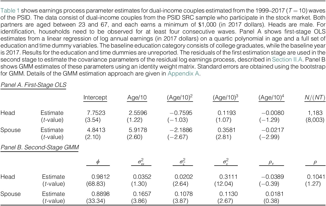
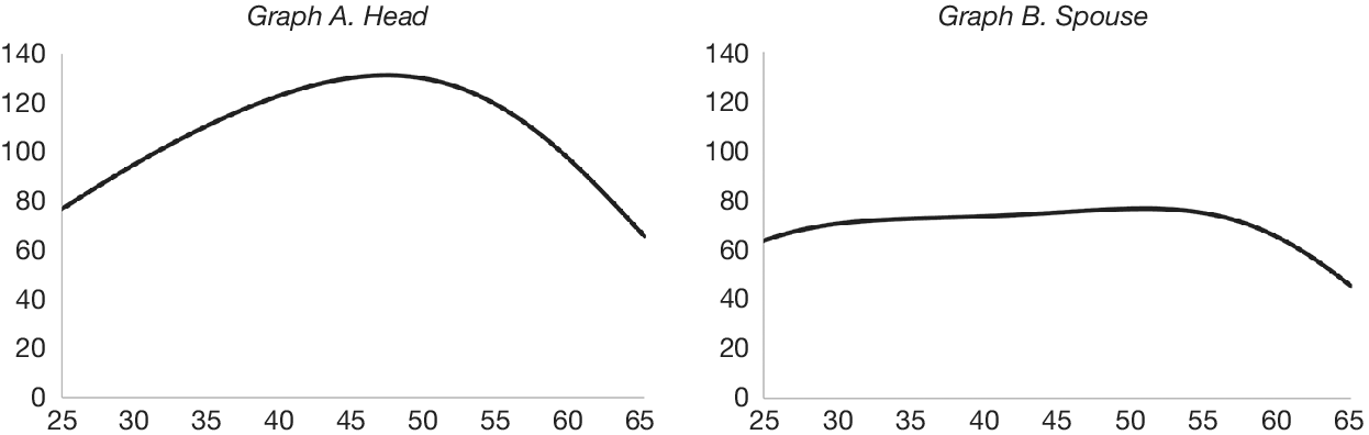

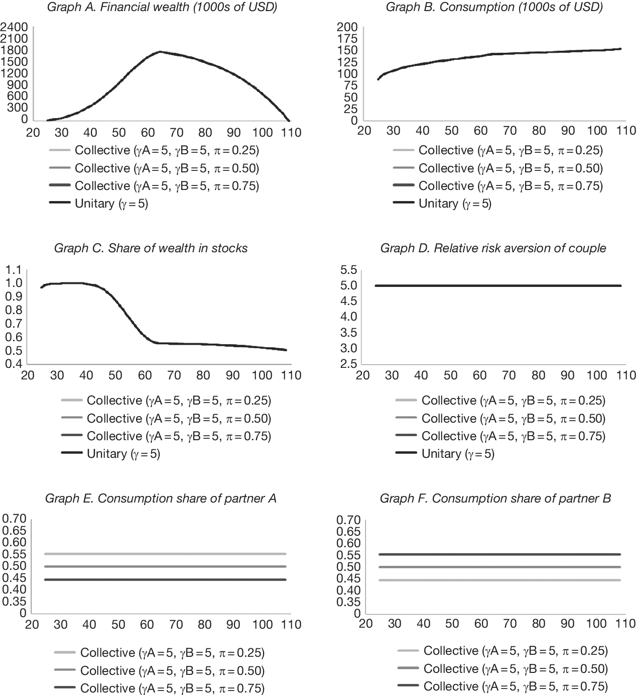


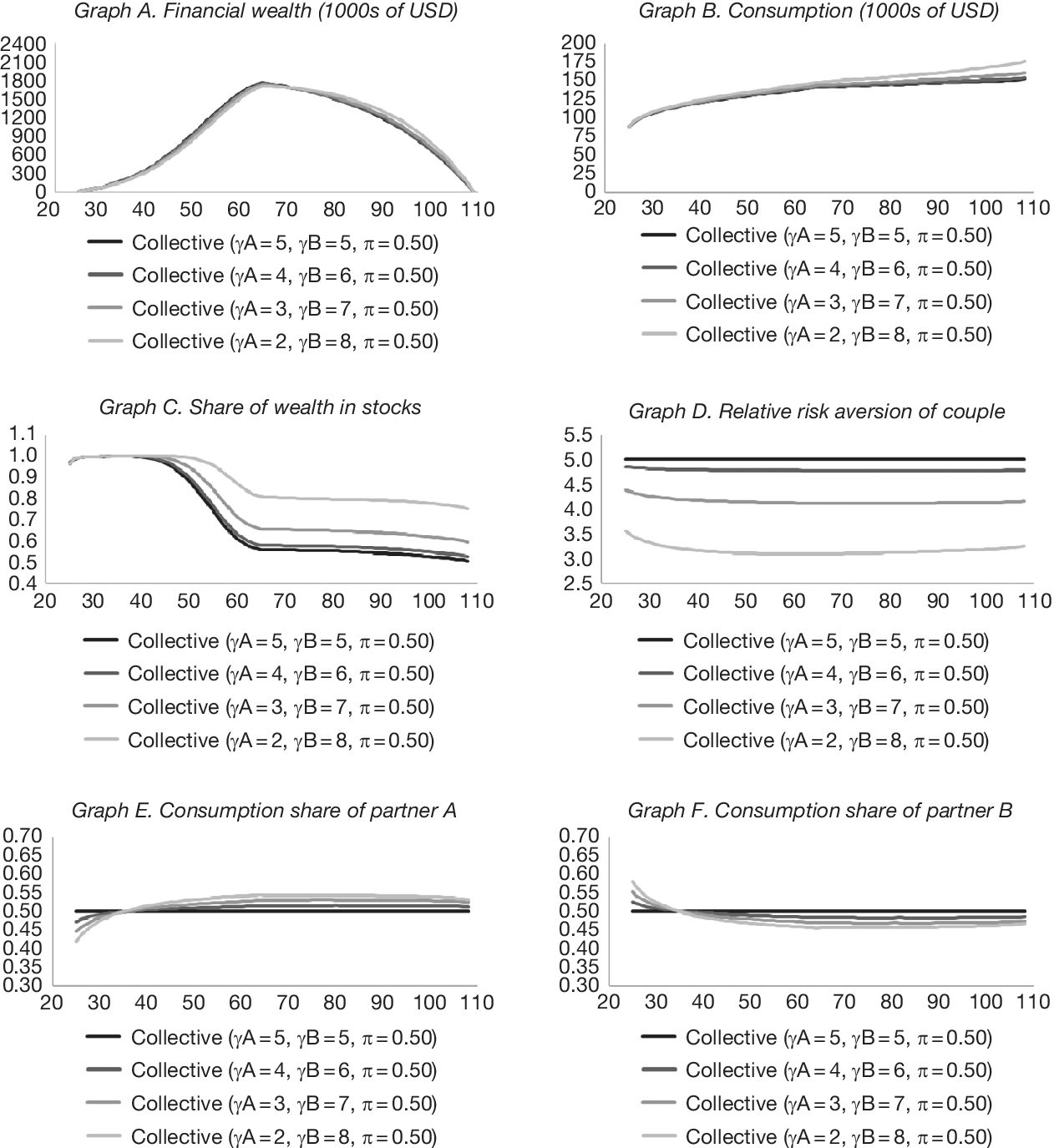


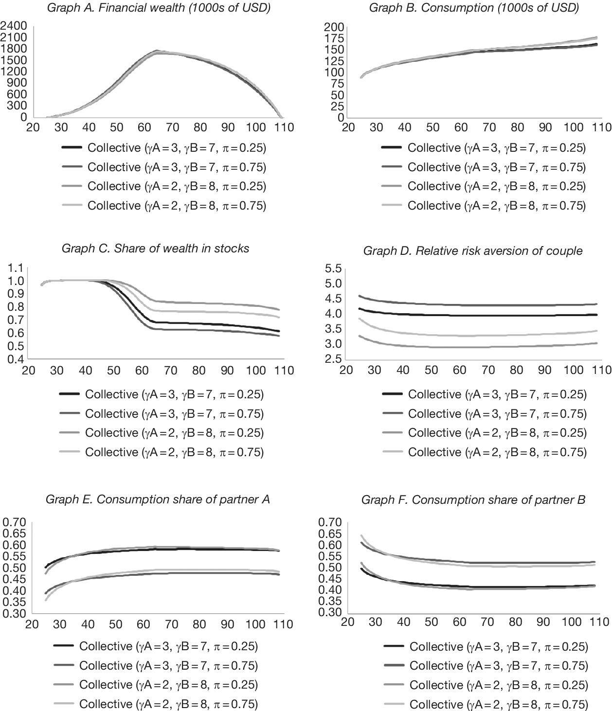


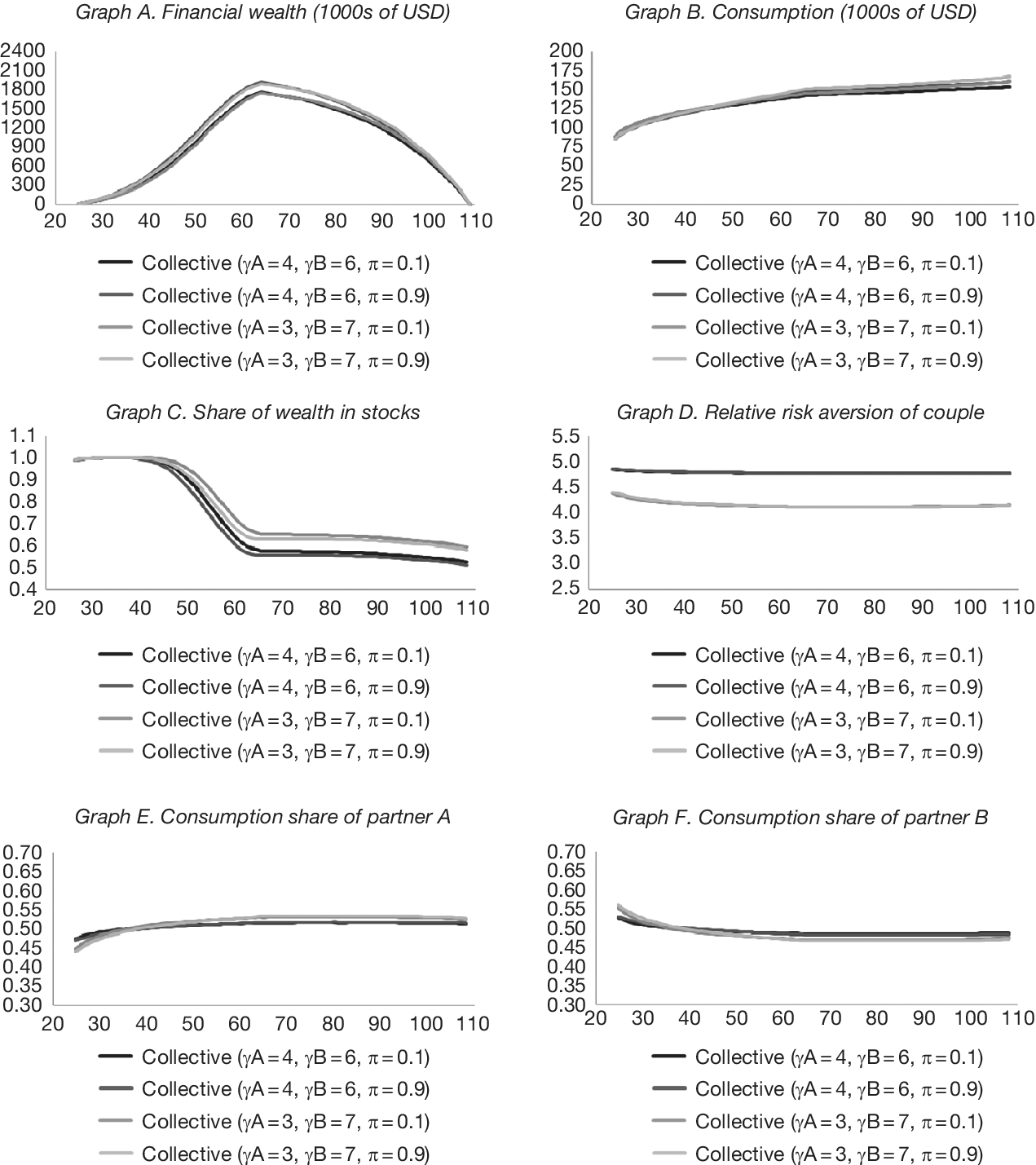


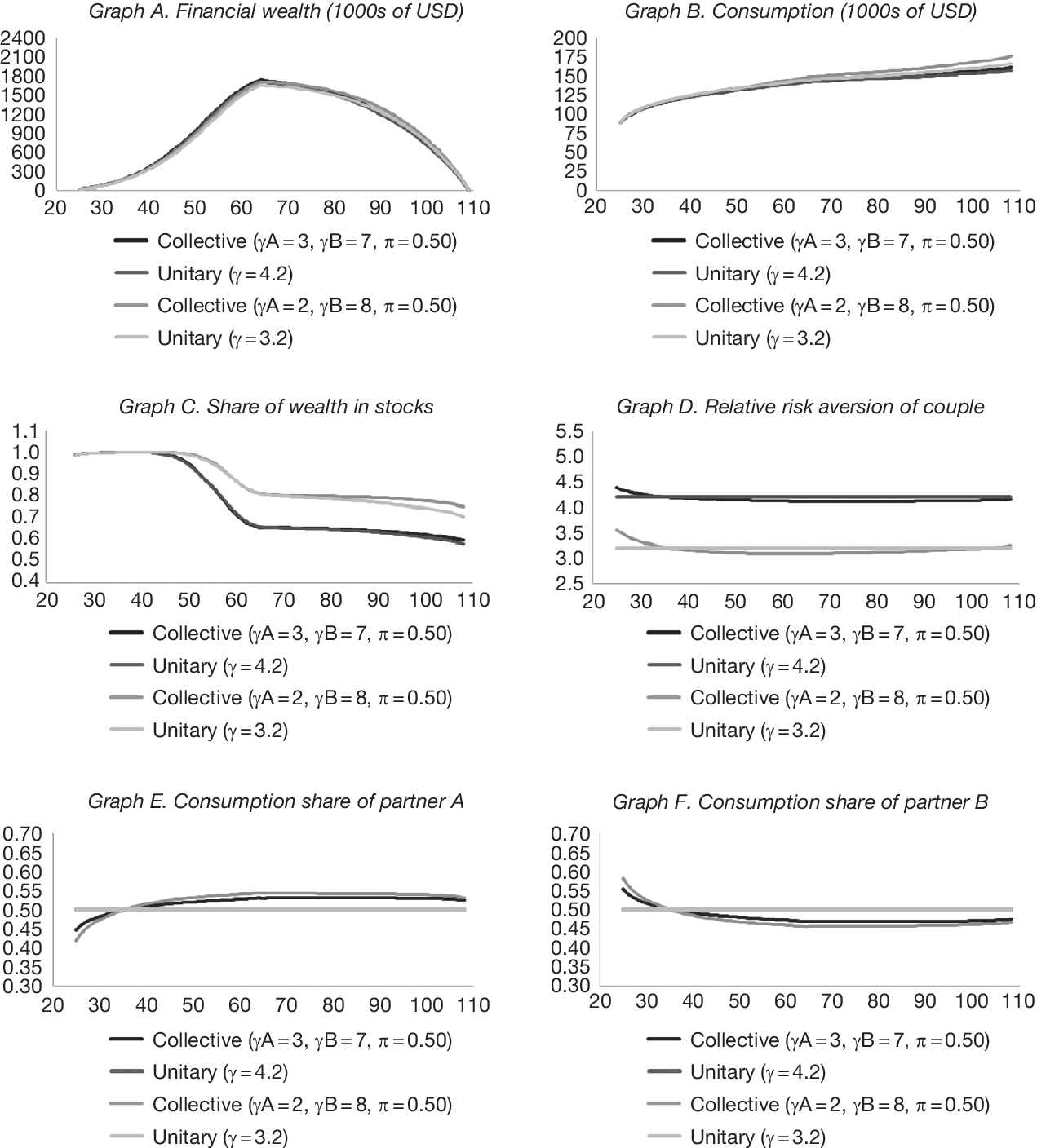


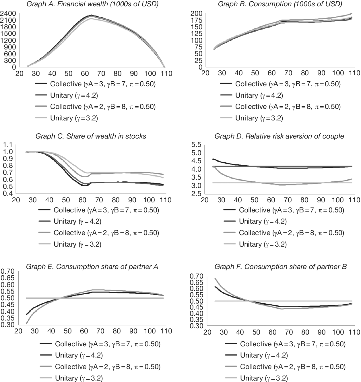


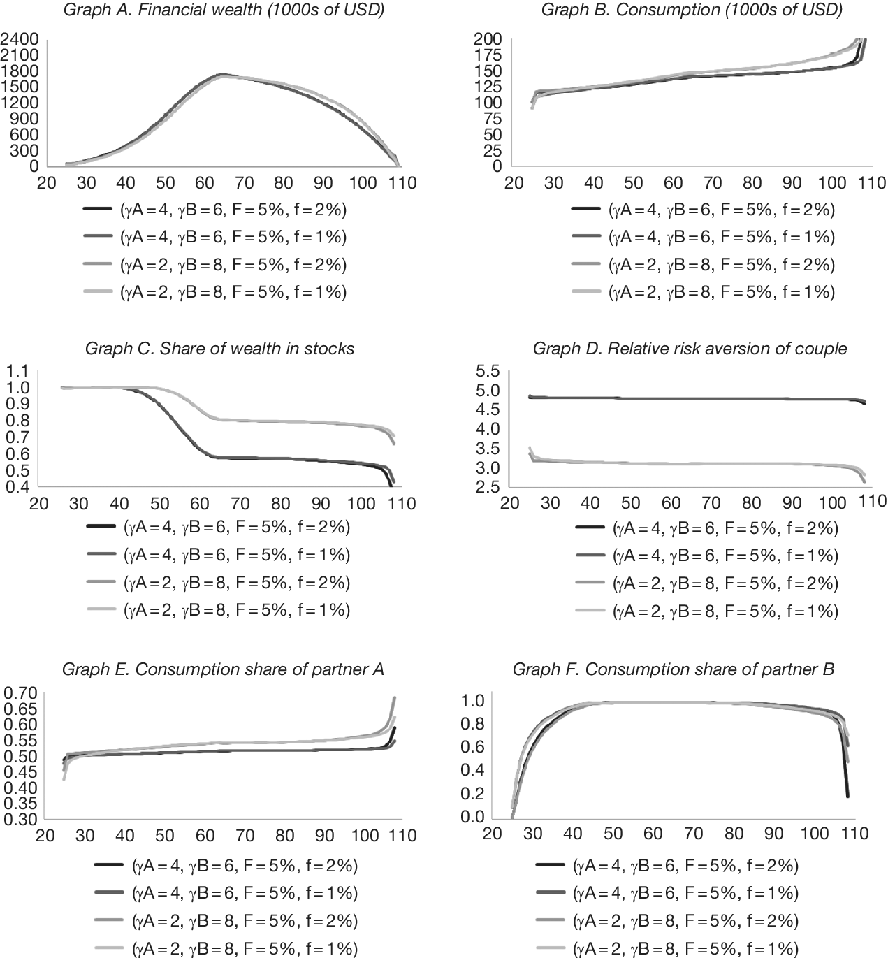


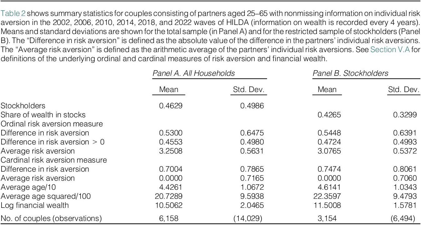
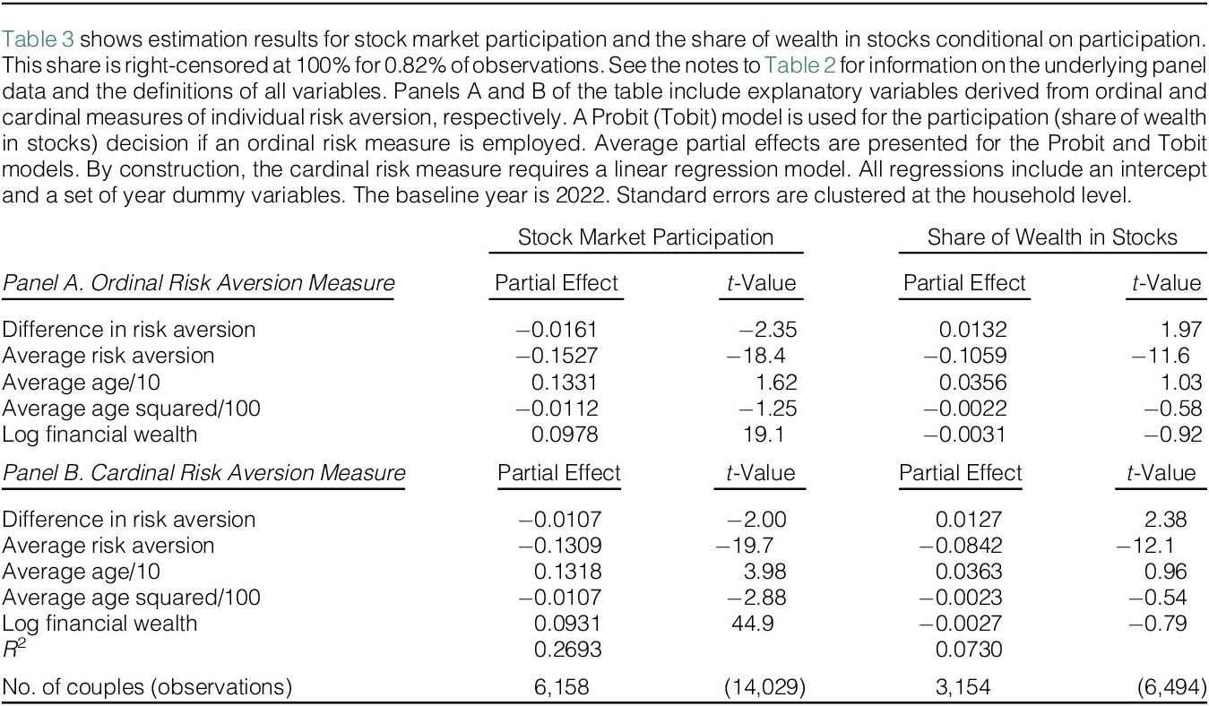

 Open access

