





1. Introduction
Droplet impact on solid surfaces is one of the most common fluid phenomena in nature, and research into its dynamics can be traced back more than a century (Worthington Reference Worthington1908). Generally, droplet impact dynamics is determined by surface configurations (e.g. surface geometry, wettability) and impact conditions (e.g. fluid properties, impact velocity) (Yarin Reference Yarin2006; Yu et al. Reference Yu, Zhang, Hu and Luo2021; Wang et al. Reference Wang, Xu, Guo, Zhao and Chen2023c ). Depending on the combination of these parameters, droplets exhibit different impact outcomes, such as adhesion, rebound or splashing (Rioboo, Tropea & Marengo Reference Rioboo, Tropea and Marengo2001; Josserand & Thoroddsen Reference Josserand and Thoroddsen2016). Numerous studies have investigated droplet morphologies and dynamic behaviours upon impact with substrates, aiming to achieve precise control over droplet impact outcomes (Liang & Mudawar Reference Liang and Mudawar2017a ; Zhao et al. Reference Zhao, Li, Liu, Li, Xue, Yuan, Yu, Li, Deng and Song2023). Such fundamental physical understanding provides essential theoretical foundations for industrial and engineering applications, including inkjet printing (Lohse Reference Lohse2021), spray cooling (Liang & Mudawar Reference Liang and Mudawar2017b ; Gu et al. Reference Gu2025) and anti-icing (Cao et al. Reference Cao2009).
Typically, the physical properties of a flat surface, such as solid–liquid and solid–gas interfacial tensions, remain homogeneous regardless of surface structure variations (Josyula et al. Reference Josyula2024), and the three-phase contact angle is also fixed as described by Young’s equation (Young Reference Young1805). Depending on the contact angle, these surfaces can be categorised as superhydrophilic, hydrophilic, hydrophobic or superhydrophobic (Yan, Gao & Barthlott Reference Yan, Gao and Barthlott2011). Among these, superhydrophobic surfaces, inspired by natural systems such as the lotus leaf (Barthlott & Neinhuis Reference Barthlott and Neinhuis1997), have received extensive attention due to their wide-ranging applications in self-cleaning and anti-icing technologies (Rothstein Reference Rothstein2010). When a droplet impacts a superhydrophobic surface, a typical evolution process includes spreading, retraction and bouncing. The work of Richard, Clanet & Quéré (Reference Richard, Clanet and Quéré2002a ) demonstrated that the bouncing time of the droplet is independent of impact velocity and follows the Rayleigh limit (Rayleigh Reference Rayleigh1879). In recent years, numerous superhydrophobic surface designs including column structures (Girard, Soto & Varanasi Reference Girard, Soto and Varanasi2019; Ding et al. Reference Ding2021), ridge structures (Gauthier et al. Reference Gauthier2015; Guo et al. Reference Guo2018; Hu et al. Reference Hu2022) or curved structures (Liu et al. Reference Liu, Andrew, Li, Yeomans and Wang2015; Shen et al. Reference Shen, Liu, Zhu, Tao, Chen, Tao, Pan, Wang and Wang2017; Abolghasemibizaki, McMasters & Mohammadi Reference Abolghasemibizaki, McMasters and Mohammadi2018) have been proposed to reduce the solid–liquid contact time, the review by Hu et al. (Reference Hu2023) has comprehensively summarised recent progress in this field. Among these advances, the study by Liu et al. (Reference Liu, Moevius, Xu, Qian, Yeomans and Wang2014) demonstrated that superhydrophobic micropillar arrays can trigger ‘pancake bouncing,’ where the droplet lifts off in a pancake-like shape. This effect converts capillary energy stored during penetration into upward kinetic energy (KE) (Moevius et al. Reference Moevius, Liu, Wang and Yeomans2014), thereby reducing the droplet–surface contact time by up to 80 %.
However, droplets impacting homogeneous wettability surfaces usually exhibit a uniform dynamic response, such as wetting and bouncing cannot occur simultaneously for a fixed surface design, regardless of the impact conditions. This limitation means that homogeneous surfaces cannot meet the complex requirements of cutting-edge engineering applications (Li et al. Reference Li and Li2020b ; Luo et al. Reference Luo, Zhang, Zeng, Zhang, Zeng and Zhou2023). A corresponding solution is to employ heterogeneous wettability surfaces with designed patterns of hydrophobic and hydrophilic regions to meet demanding requirements (Zhu et al. Reference Zhu, Huang, Lou and Xia2019; Yang et al. Reference Yang, Xu, Zhang and Wang2020). On such surfaces, different areas possess distinct wettabilities, thereby introducing complex solid–liquid interactions that enable precise control over droplet behaviour. A typical example is the Namib desert beetle (Stenocara), which collects and transports water for survival in the Namib Desert through a heterogeneous wettability strategy (Parker & Lawrence Reference Parker and Lawrence2001). This concept has greatly inspired the design and application of heterogeneous wettability in a variety of fields such as optical and electronic device fabrication (Leng et al. Reference Leng2018; Abe et al. Reference Abe2020), cellular interactions (Li et al. Reference Li2015; Leite et al. Reference Leite2017; Feng, Ueda & Levkin Reference Feng, Ueda and Levkin2018) and biosensing (Huang et al. Reference Huang2013; Li et al. Reference Li and Fang2020a ). Nevertheless, most existing studies on droplet impact on homogeneous wettability surfaces focus on applications and fabrication techniques (Li et al. Reference Li and Li2020b ), with relatively few addressing the impact dynamics or developing surface design criteria for determining droplet bouncing behaviours from a fluid mechanics perspective.
In recent years, droplet dynamics on structured surfaces have received extensive research attention (Wang, Wu & Nestler Reference Wang, Wu and Nestler2023a ; Wang et al. Reference Wang, Xu, Guo, Zhao and Chen2023c ), particularly on micropillar-structured surfaces, which are considered a typical design for achieving superhydrophobicity (Quéré Reference Quéré2002; Yoshimitsu et al. Reference Yoshimitsu, Nakajima, Watanabe and Hashimoto2002). One key issue in the research of droplet dynamics on pillar-structured surfaces is determining the critical conditions for the transition between the Wenzel state and the Cassie state (Lafuma & Quéré Reference Lafuma and Quéré2003; Reyssat & Quéré Reference Reyssat and Quéré2009). For example, both Deng et al. (Reference Deng2009) and Chen et al. (Reference Chen2011) suggested that, for impacting droplets, the criterion for achieving either the Wenzel state or the Cassie state is determined by balancing hammer pressure, dynamic pressure and capillary pressure. Murakami, Jinnai & Takahara (Reference Murakami, Jinnai and Takahara2014) developed an energy barrier model describing the energy landscape from the Cassie state to the Wenzel state, demonstrating that the transition is primarily dictated by the competition between the energy barrier and the Laplace pressure. On the other hand, some recent studies have reported droplet dynamics on surfaces with composite wettability, such as superhydrophobic dots (Lenz & Lipowsky Reference Lenz and Lipowsky1998; Majhy, Singh & Sen Reference Majhy, Singh and Sen2020), stripes (Bliznyuk et al. Reference Bliznyuk2009; Jansen et al. Reference Jansen2012; Wang et al. Reference Wang, Zhao, Zhang, Jian, Liu and Zhang2019; Wu et al. Reference Wu, Wang, Selzer and Nestler2019) or patterns (Kusumaatmaja & Yeomans Reference Kusumaatmaja and Yeomans2007; Wu et al. Reference Wu, Wang, Ma, Selzer and Nestler2020, Reference Wu, Wang, Ma, Selzer and Nestler2022) on hydrophilic substrates. However, these surfaces are mostly two-dimensional in design, and the research focus has been on droplet wetting behaviours (Wang et al. Reference Wang, Wu and Nestler2023a ). Studies on the droplet impact dynamics on three-dimensional micropillar-structured surfaces with heterogeneous wettability remain absent.
Usually, fabricating three-dimensional heterogeneous wettability surfaces is complex and costly (Li et al. Reference Li and Li2020b ; Luo et al. Reference Luo, Zhang, Zeng, Zhang, Zeng and Zhou2023). In particular, variations in the geometry and wettability contrast of microstructures can have a significant influence on droplet impact outcomes, which poses challenges for experiments. As an alternative, numerical simulations offer ‘controlled numerical experiments’, in which all geometric, physical and operating parameters can be specified precisely and easily while the complete dynamic process, in addition to the impact outcomes, can be studied under various conditions. Especially in studies of droplet dynamics on micropillar surfaces, numerical simulations can provide the opportunity to observe highly transient interfacial evolution within micropillar gaps at the microscale and to obtain quantitative data such as velocity distributions (Xia et al. Reference Xia, Yang, Chen, Liu, Tian and Zhang2024). In recent years, the lattice Boltzmann method (LBM) has emerged as a powerful and efficient computational fluid dynamics tool, particularly well suited for simulating multiphase flows with complex boundary geometries due to its inherent collision–streaming mechanism (Li et al. Reference Li2016; Hosseini & Karlin Reference Hosseini and Karlin2023). However, conventional multiphase LBM models are limited in their accessible parameter ranges, such as density and viscosity ratios (Aidun & Clausen Reference Aidun and Clausen2010). In response, many recent studies have focused on proposing advanced collision operators (Mazloomi, Chikatamarla & Karlin Reference Mazloomi, Chikatamarla and Karlin2015; Bösch, Dorschner & Karlin Reference Bösch, Dorschner and Karlin2018; Fei, Luo & Li Reference Fei, Luo and Li2018) and multiphase models (Li, Luo & Li Reference Li, Luo and Li2012; Geier, Fakhari & Lee Reference Geier, Fakhari and Lee2015; Wöhrwag et al. Reference Wöhrwag, Semprebon, Mazloomi Moqaddam, Karlin and Kusumaatmaja2018) to extend the boundary of simulation parameters. To facilitate flexible switching between different collision operators and to enable the extension of advanced models across various collision schemes, Luo, Fei & Wang (Reference Luo, Fei and Wang2021) have proposed a unified lattice Boltzmann (ULBM). Within this framework, multiphase flow models can be constructed according to specific simulation requirements, allowing for an optimal balance between computational efficiency and capability (Wang, Fei & Luo Reference Wang, Fei and Luo2022; Wang et al. Reference Wang2023b ).
In recent years, the LBM has been employed to simulate droplet impact on striped surfaces with heterogeneous wettability, enabling systematic studies of droplet splitting and spreading dynamics (Lee et al. Reference Lee2017; He et al. Reference He2024). However, current research on droplet impact dynamics on heterogeneous wettability surfaces remains insufficient to meet the broad range of application requirements. In particular, in biomedical fields, there is an urgent need to design surfaces that enable selective bouncing or wetting of droplets under different impact conditions for applications such as cell screening (Chen & Zhang Reference Chen and Zhang2020; Li et al. Reference Li and Li2020b ). To this end, we propose a heterogeneous wettability surface design composed of superhydrophobic micropillars on a hydrophilic substrate to achieve selective bouncing or wetting of impacting droplets. A force balance analysis of droplet penetration processes within the micropillar array is conducted, and a predictive model for droplet penetration is proposed. Then a systematic LBM simulation of the droplet impingement is performed, we demonstrate that droplets impacting such surfaces can exhibit four distinct outcomes: pancake bouncing, complete bouncing, partial wetting and complete wetting. We establish predictive criteria for the different impact outcomes through a proposed analytical model and perform an energy analysis of the droplet evolution. The paper is organised as follows, § 2 outlines the numerical methods and simulation set-up, § 3 presents the results and discussion, the conclusion is provided in § 4.
2. Numerical methods and set-up
2.1. Model description
To simulate the two-phase flow, a non-orthogonal phase-field (PF) model is employed. In the PF model, an improved conservative Allen–Cahn (AC) equation is used for interface tracking (Chiu & Lin Reference Chiu and Lin2011), i.e.
 \begin{equation} \begin{array}{c} \frac{\partial \phi }{\partial t}+\boldsymbol{\nabla }\boldsymbol{\cdot }\left(\phi \boldsymbol{u}\right)=\boldsymbol{\nabla }\boldsymbol{\cdot }M_{\phi }\left(\boldsymbol{\nabla }\phi -\frac{\boldsymbol{n}}{w_{in}}\left[1-\tanh ^{2}\left(\frac{2{T }}{W_{\textit{in}}}\right)\right]\right)\!, \end{array} \end{equation}
where $\phi$
is the phase indicator, for the liquid phase
$\phi$
is the phase indicator, for the liquid phase $\phi _{l}=1$
and for the gas phase
$\phi _{l}=1$
and for the gas phase $\phi _{g}=0$
, with
$\phi _{g}=0$
, with $\phi _{0}=(\phi _{l}+\phi _{g})/2=0.5$
indicating the position of the interface;
$\phi _{0}=(\phi _{l}+\phi _{g})/2=0.5$
indicating the position of the interface; $\boldsymbol{n}=\boldsymbol{\nabla }\phi /| \boldsymbol{\nabla }\phi |$
is the unit vector normal to the interface;
$\boldsymbol{n}=\boldsymbol{\nabla }\phi /| \boldsymbol{\nabla }\phi |$
is the unit vector normal to the interface; $M_{\phi }$
is the mobility and
$M_{\phi }$
is the mobility and $W_{\textit{in}}$
stands for the interface thickness. In this work, unless otherwise specified,
$W_{\textit{in}}$
stands for the interface thickness. In this work, unless otherwise specified, $W_{\textit{in}}$
is set to 5 lattices. Here
$W_{\textit{in}}$
is set to 5 lattices. Here $\boldsymbol{u}=[u_{x},\,u_{y},\,u_{z}]$
is the fluid velocity. A signed-distance function
$\boldsymbol{u}=[u_{x},\,u_{y},\,u_{z}]$
is the fluid velocity. A signed-distance function ${T }$
is introduced to avoid any jumps or discontinuities at the interface (Jain Reference Jain2022; Liang et al. Reference Liang2023), where
${T }$
is introduced to avoid any jumps or discontinuities at the interface (Jain Reference Jain2022; Liang et al. Reference Liang2023), where
 \begin{equation} \begin{array}{c} {T }=\frac{W_{\textit{in}}}{4}\ln \left(\frac{\phi }{1-\phi }\right)\!.\end{array} \end{equation}
For the PF multiphase model, the conservative AC equation is coupled with incompressible Navier–Stokes (NS) equations, where the fluid flow is described as (Unverdi & Tryggvason Reference Unverdi and Tryggvason1992)
 \begin{align} \boldsymbol{\nabla }\boldsymbol{\cdot }\boldsymbol{u}&=0,\notag\\ \frac{\partial \left(\rho \boldsymbol{u}\right)}{\partial t}+\boldsymbol{\nabla }\boldsymbol{\cdot }\left(\rho \boldsymbol{uu}\right)&=-\boldsymbol{\nabla }P+\boldsymbol{\nabla }\boldsymbol{\cdot }\left(\rho \nu \left(\boldsymbol{\nabla }\boldsymbol{u}+\boldsymbol{\nabla }\boldsymbol{u}^{T}\right)+\rho \left(\nu _{b}-\frac{2}{3}\nu \right)\left(\boldsymbol{\nabla }\boldsymbol{\cdot }\boldsymbol{u}\right)\boldsymbol{I}\right)\notag\\&\quad +\boldsymbol{F}_{\boldsymbol{s}}+\boldsymbol{F}_{\boldsymbol{b}}, \end{align}
with $\rho$
the fluid density,
$\rho$
the fluid density, $\nu$
the fluid kinematic viscosity,
$\nu$
the fluid kinematic viscosity, $\nu _{b}$
represents the non-hydrodynamic bulk viscosity and
$\nu _{b}$
represents the non-hydrodynamic bulk viscosity and $P$
is the pressure;
$P$
is the pressure; $\boldsymbol{F}_{\boldsymbol{s}}$
,
$\boldsymbol{F}_{\boldsymbol{s}}$
, $\boldsymbol{F}_{\boldsymbol{b}}$
are the surface tension and external body force, respectively:
$\boldsymbol{F}_{\boldsymbol{b}}$
are the surface tension and external body force, respectively:
 \begin{align} \boldsymbol{F}_{\boldsymbol{s}}&=\mu _{\phi }\boldsymbol{\nabla }\phi ,\notag\\ \boldsymbol{F}_{\boldsymbol{b}}&=\boldsymbol{g}\rho . \end{align}
Here $\boldsymbol{g}$
is gravity and
$\boldsymbol{g}$
is gravity and $\mu _{\phi }=4\beta (\phi -\phi _{l})(\phi -\phi _{g})(\phi -\phi _{0})-k\boldsymbol{\nabla} ^{2}\phi$
is the chemical potential, the surface tension
$\mu _{\phi }=4\beta (\phi -\phi _{l})(\phi -\phi _{g})(\phi -\phi _{0})-k\boldsymbol{\nabla} ^{2}\phi$
is the chemical potential, the surface tension $\gamma$
is related to the parameters
$\gamma$
is related to the parameters $\beta =12\gamma /w_{in}$
and
$\beta =12\gamma /w_{in}$
and $k=3\gamma w_{in}/2$
.
$k=3\gamma w_{in}/2$
.
In this study, the ULBM is adopted to solve the above governing equations, where the collision equation for the multiple relaxation time (MRT) ULBM model can be expressed as (Luo et al. Reference Luo, Fei and Wang2021)
 \begin{align} f_{i}\left(\boldsymbol{x}+\boldsymbol{e}_{i}{\unicode[Arial]{x0394}} t,t+{\unicode[Arial]{x0394}} t\right)&={f}_{i}^{{*}}\left(\boldsymbol{x},t\right)= \boldsymbol{M}^{-1}\left(\boldsymbol{I}-\boldsymbol{S}\right)\boldsymbol{M}f_{i}\left(\boldsymbol{x},t\right)\notag\\&\quad+\boldsymbol{M}^{-1}\boldsymbol{SM}{f}_{i}^{eq}\left(\boldsymbol{x},t\right)+{\unicode[Arial]{x0394}} t\boldsymbol{M}^{-1}\left(\boldsymbol{I}-\frac{\boldsymbol{S}}{2}\right)\boldsymbol{M}C_{i}, \end{align}
where $f_{i}\,$
and
$f_{i}\,$
and ${f}_{i}^{{*}}$
are the pre-collision and post-collision distribution functions, respectively,
${f}_{i}^{{*}}$
are the pre-collision and post-collision distribution functions, respectively, ${\,f}_{i}^{eq}$
is the equilibrium distribution function and
${\,f}_{i}^{eq}$
is the equilibrium distribution function and $C_{i}$
is the external forcing term,
$C_{i}$
is the external forcing term, $\boldsymbol{e}_{i}$
and
$\boldsymbol{e}_{i}$
and ${\unicode[Arial]{x0394}} t=1$
are the discrete velocities and the time step, respectively, and
${\unicode[Arial]{x0394}} t=1$
are the discrete velocities and the time step, respectively, and $\boldsymbol{I}$
stands for the unit matrix.
$\boldsymbol{I}$
stands for the unit matrix.
To capture the realistic dynamic behaviours of droplets in three dimensions, the D3Q19 discrete velocity model is adopted. Two different distribution functions are introduced to solve the conservation AC equation and the incompressible NS equations:
 \begin{equation} \begin{array}{c} {\boldsymbol{m}}_{\phi }^{{*}}=\left(\boldsymbol{I}-\boldsymbol{S}_{\phi }\right)\boldsymbol{m}_{\phi }+\boldsymbol{S}_{\phi }{\boldsymbol{m}}_{\phi }^{\boldsymbol{eq}}+{\unicode[Arial]{x0394}} t\left(\boldsymbol{I}-\frac{\boldsymbol{S}_{\phi }}{2}\right)\boldsymbol{R}_{{\unicode[Arial]{x03D5}} },\\ {\boldsymbol{m}}_{g}^{{*}}=\left(\boldsymbol{I}-\boldsymbol{S}_{g}\right)\boldsymbol{m}_{g}+\boldsymbol{S}_{g}{\boldsymbol{m}}_{g}^{eq}+{\unicode[Arial]{x0394}} t\left(\boldsymbol{I}-\frac{\boldsymbol{S}_{g}}{2}\right)\boldsymbol{R}_{g} .\end{array} \end{equation}
Here $\boldsymbol{m}_{\phi }=\boldsymbol{M}f_{\phi ,i}$
is for the conservation AC equation and
$\boldsymbol{m}_{\phi }=\boldsymbol{M}f_{\phi ,i}$
is for the conservation AC equation and $\boldsymbol{m}_{g}=\boldsymbol{M}{\kern-1pt}g_{i}$
is for the incompressible NS equations. For the non-orthogonal MRT collision operator, the transformation matrix
$\boldsymbol{m}_{g}=\boldsymbol{M}{\kern-1pt}g_{i}$
is for the incompressible NS equations. For the non-orthogonal MRT collision operator, the transformation matrix $\boldsymbol{M}$
is chosen as the simplified non-orthogonal moment set that was originally proposed by Fei et al. (Reference Fei, Luo and Li2018, Reference Fei2019). In (2.6) the discrete equilibrium moment sets and the discrete forcing terms such as
$\boldsymbol{M}$
is chosen as the simplified non-orthogonal moment set that was originally proposed by Fei et al. (Reference Fei, Luo and Li2018, Reference Fei2019). In (2.6) the discrete equilibrium moment sets and the discrete forcing terms such as ${\boldsymbol{m}}_{\phi }^{eq}=\boldsymbol{M}{f}_{\phi ,i}^{eq}$
,
${\boldsymbol{m}}_{\phi }^{eq}=\boldsymbol{M}{f}_{\phi ,i}^{eq}$
, ${\boldsymbol{m}}_{g}^{eq}=\boldsymbol{M}{g}_{i}^{eq}$
,
${\boldsymbol{m}}_{g}^{eq}=\boldsymbol{M}{g}_{i}^{eq}$
, $\boldsymbol{R}_{g}=\boldsymbol{M}C_{g,i}\,$
and
$\boldsymbol{R}_{g}=\boldsymbol{M}C_{g,i}\,$
and $\boldsymbol{R}_{\phi }=\,\boldsymbol{M}{\kern-1pt}C_{\phi ,i}$
are given explicitly in our previous work (Wang et al. Reference Wang2023b
). After the collision step in raw moment space (2.6), the distribution functions can be reconstructed as
$\boldsymbol{R}_{\phi }=\,\boldsymbol{M}{\kern-1pt}C_{\phi ,i}$
are given explicitly in our previous work (Wang et al. Reference Wang2023b
). After the collision step in raw moment space (2.6), the distribution functions can be reconstructed as $g_{i}=\boldsymbol{M}^{-1}{\boldsymbol{m}}_{g}^{{*}}$
and
$g_{i}=\boldsymbol{M}^{-1}{\boldsymbol{m}}_{g}^{{*}}$
and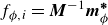 $f_{\phi ,i}=\boldsymbol{M}^{-1}{\boldsymbol{m}}_{\phi }^{\boldsymbol{*}}$
.
$f_{\phi ,i}=\boldsymbol{M}^{-1}{\boldsymbol{m}}_{\phi }^{\boldsymbol{*}}$
.
To model the wetting behaviours involved in the following cases, we employed an energy-based contact angle model, in which the relationship between the solid phase indicator ( $\phi _{s}$
) and the apparent contact angle (
$\phi _{s}$
) and the apparent contact angle ( $\theta$
) can be expressed as (Zarareh et al. Reference Zarareh, Khajepor, Burnside and Chen2021)
$\theta$
) can be expressed as (Zarareh et al. Reference Zarareh, Khajepor, Burnside and Chen2021)
 \begin{equation} \begin{array}{c} \boldsymbol{n}\boldsymbol{\cdot }\boldsymbol{\nabla }\phi _{s}=\,-\sqrt{\frac{2\beta }{\kappa }}\phi _{s}\left(1\,-\,\phi _{s}\right)\cos \theta . \end{array} \end{equation}
In the following simulations the solid boundaries are implemented as no-slip for the fluid momentum, while the singularity at the moving contact line is regularised by the diffuse-interface PF model (Jacqmin Reference Jacqmin2000; Yue, Zhou & Feng Reference Yue, Zhou and Feng2010). In the present study, a static contact angle model is adopted without considering contact angle hysteresis, since our focus is on droplet impingement dynamics rather than on the detailed evolution of the moving contact line. This modelling assumption leads to a significantly simplified treatment and is sufficient for the present purpose, as supported by the comparison between simulations and experiments shown in § 2.2. The effects associated with detailed moving-contact-line physics, which may become important on hydrophilic surfaces or surfaces with significant contact angle hysteresis, will be addressed in future work. The above contact angle model can be used to simulate complex surfaces with a wide range of wettabilities. Detailed validations are provided in Appendix A. The above ULBM PF model was implemented in C++ and parallelised using the message passing interface. It has been integrated into our in-house software suite UCLBM (unified cascaded LBM). We have used this model to simulate a range of complex multiphase flow behaviours, such as phase change multiphase flow in porous media (Yang et al. Reference Yang, Xu, Kou, Wang, Lei, Wang, Li and Luo2024) and droplet breakup in electric fields (Wang et al. Reference Wang, Lei, Yang, Fei, Chen and Luo2024).
2.2. Comparison with experiments
Before simulating the main cases, we first validated the numerical model in the above section. Specifically, we conducted a validation and mesh convergence study by simulating the impingement of a water droplet on a flat superhydrophobic surface and comparing the results with the experiments by Zhang et al. (Reference Zhang2022). The initial droplet radius was set to ${R}_{0}=1.05\,{\rm mm}$
, the impact Weber number
${R}_{0}=1.05\,{\rm mm}$
, the impact Weber number ${\textit{We}}=\rho _{l}R_{0}{{V}}_{0}^{2}/\sigma$
was 20 and the superhydrophobic surface had a contact angle of
${\textit{We}}=\rho _{l}R_{0}{{V}}_{0}^{2}/\sigma$
was 20 and the superhydrophobic surface had a contact angle of $\theta _{0}=165^{\circ}$
. The liquid phase is water and the gas phase is air, with their properties listed in table 1. The simulation domain is set as a rectangular box of size
$\theta _{0}=165^{\circ}$
. The liquid phase is water and the gas phase is air, with their properties listed in table 1. The simulation domain is set as a rectangular box of size $L_{x}\times L_{y}\times L_{z}=300\times 300\times 600$
. Considering the symmetric nature of the problem, planar symmetry boundary conditions are imposed at
$L_{x}\times L_{y}\times L_{z}=300\times 300\times 600$
. Considering the symmetric nature of the problem, planar symmetry boundary conditions are imposed at $L_{x}=0$
and
$L_{x}=0$
and $L_{y}=0$
. Figure 1(a) presents the time evolution of the spreading radius for different grid resolutions, the results demonstrate that the grid is sufficiently fine when
$L_{y}=0$
. Figure 1(a) presents the time evolution of the spreading radius for different grid resolutions, the results demonstrate that the grid is sufficiently fine when ${\rm d}x\leq R_{0}/45$
, and the mesh size has negligible influence on the final results. During the evolution, the average relative error between the simulation and the experiment is about 8 %, with the maximum error occurring at the point of maximum spreading diameter. This may be attributed to the absence of contact angle hysteresis effects in our simulation. Figure 1(b) presents qualitative comparison snapshots of our simulation results (left, blue) and the experimental results (right, black). It can be seen that our simulation accurately captures the droplet dynamics, including the splitting of a satellite droplet at
${\rm d}x\leq R_{0}/45$
, and the mesh size has negligible influence on the final results. During the evolution, the average relative error between the simulation and the experiment is about 8 %, with the maximum error occurring at the point of maximum spreading diameter. This may be attributed to the absence of contact angle hysteresis effects in our simulation. Figure 1(b) presents qualitative comparison snapshots of our simulation results (left, blue) and the experimental results (right, black). It can be seen that our simulation accurately captures the droplet dynamics, including the splitting of a satellite droplet at $t=9.1\,{\rm ms}$
.
$t=9.1\,{\rm ms}$
.
Comparison between simulation and experimental results for a water droplet impacting a flat superhydrophobic surface at We = 20: (a) time evolution of the droplet radius for various mesh sizes; (b) comparison of droplet morphology.

Figure 1. Long description
The image contains two parts: (a) a line graph and (b) a series of images. Part (a) shows the time evolution of the droplet radius for various mesh sizes. The x-axis represents time in milliseconds, and the y-axis represents the droplet radius in millimeters. The graph includes experimental data points and three simulation lines for different mesh sizes: dx equals R0/60, dx equals R0/50, and dx equals R0/45. Part (b) shows a comparison of droplet morphology at different time points: t equals 0 milliseconds, t equals 0.3 milliseconds, t equals 2.4 milliseconds, t equals 4.8 milliseconds, and t equals 9.1 milliseconds. The images depict the droplet's shape and behavior as it impacts the surface.
Fluid properties in current simulations.

Table 1. Long description
A table with two rows and three columns compares fluid properties in current simulations. The columns are labeled Density, Dynamic viscosity, and Surface tension. The gas phase has a density of 1.17 kilograms per cubic meter, a dynamic viscosity of 18.45 micropascal seconds, and a surface tension of 0.072 newtons per meter. The liquid phase has a density of 997.05 kilograms per cubic meter and a dynamic viscosity of 890.08 micropascal seconds. The table highlights the differences in physical properties between the gas and liquid phases used in the simulations.
To validate the accuracy of the adopted ULBM (PF) model in capturing droplet dynamics on microstructured surfaces, a comparative study was conducted between simulation results and experimental data (Liu et al. Reference Liu, Moevius, Xu, Qian, Yeomans and Wang2014). We first reproduced the experiment of a water droplet impacting a pillared superhydrophobic surface at two different Weber numbers, We = 4.7 and We = 7.9, using the same pillar geometry as in the experimental set-up (Liu et al. Reference Liu, Moevius, Xu, Qian, Yeomans and Wang2014). In this case, the simulation domain and boundary conditions are identical to those in figure 1. A mesh resolution of ${\rm d}x=R_{0}/43$
is employed to match the experimental ratio of droplet radius to micropillar size. Figure 2(a) shows the evolution of droplet bouncing morphologies, where the left (blue) side displays the simulation results and the right (black) side presents the experimental snapshots (Liu et al. Reference Liu, Moevius, Xu, Qian, Yeomans and Wang2014). It can be found that, for the case at We = 4.7, the droplet exhibits a typical complete rebound morphology, undergoing spreading, retraction and rebounding after contacting the surface. Consistent with Rayleigh’s theory (Richard, Clanet & Quéré Reference Quéré2002b
; Strutt Reference Strutt2011), the droplet–surface contact time is approximately
${\rm d}x=R_{0}/43$
is employed to match the experimental ratio of droplet radius to micropillar size. Figure 2(a) shows the evolution of droplet bouncing morphologies, where the left (blue) side displays the simulation results and the right (black) side presents the experimental snapshots (Liu et al. Reference Liu, Moevius, Xu, Qian, Yeomans and Wang2014). It can be found that, for the case at We = 4.7, the droplet exhibits a typical complete rebound morphology, undergoing spreading, retraction and rebounding after contacting the surface. Consistent with Rayleigh’s theory (Richard, Clanet & Quéré Reference Quéré2002b
; Strutt Reference Strutt2011), the droplet–surface contact time is approximately $t_{c}/\,t_{\sigma }\approx 2.2,$
where the inertial capillary time
$t_{c}/\,t_{\sigma }\approx 2.2,$
where the inertial capillary time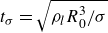 $\,t_{\sigma }=\sqrt{\rho _{l}{R}_{0}^{3}/\sigma }$
. For the case at We = 7.9, part of the droplet overcomes the capillary resistance between the superhydrophobic micropillars and penetrates into the pillar gaps. In this process, the KE is partially converted into surface energy (SE) and then the penetrated portion is rapidly expelled from the pillar gaps, resulting in a shortened liquid–solid contact time of approximately
$\,t_{\sigma }=\sqrt{\rho _{l}{R}_{0}^{3}/\sigma }$
. For the case at We = 7.9, part of the droplet overcomes the capillary resistance between the superhydrophobic micropillars and penetrates into the pillar gaps. In this process, the KE is partially converted into surface energy (SE) and then the penetrated portion is rapidly expelled from the pillar gaps, resulting in a shortened liquid–solid contact time of approximately $t_{c}/\,t_{\sigma }\approx \,0.65$
. In addition, we have verified that the results for droplet impact on micropillar surfaces are independent of both grid resolution and interface width, details can be found in Appendix B.
$t_{c}/\,t_{\sigma }\approx \,0.65$
. In addition, we have verified that the results for droplet impact on micropillar surfaces are independent of both grid resolution and interface width, details can be found in Appendix B.
Comparison between simulations and experimental results for a water droplet impacting on a pillared superhydrophobic surface at different We. (a) Qualitative comparison of droplet bouncing morphologies. (b) Quantitative comparison of contact time ( $t_{c}$
), maximum time (
$t_{c}$
), maximum time ( $t_{max}$
) and rebound factor (Q).
$t_{max}$
) and rebound factor (Q).

Figure 2. Long description
The image contains two graphs comparing simulations and experimental results of a water droplet impacting a pillared superhydrophobic surface at different Weber numbers. The first graph (a) shows a qualitative comparison of droplet bouncing morphologies at two different Weber numbers, 4.7 and 7.9. Each Weber number is represented by a series of images taken at different time intervals, illustrating the droplet's shape and position as it impacts and bounces off the surface. The second graph (b) presents a quantitative comparison of contact time, maximum time, and rebound factor as functions of the Weber number. The contact time and maximum time are plotted on the left y-axis in milliseconds, while the rebound factor is plotted on the right y-axis. The data points for experiments and simulations are distinguished by different symbols and colors. The contact time decreases with increasing Weber number, while the rebound factor shows a non-monotonic trend. The maximum time remains relatively constant across the range of Weber numbers. All values are approximated.
We then extended our simulations to a wider range of We and quantitatively compared the results with experimental data (Liu et al. Reference Liu, Moevius, Xu, Qian, Yeomans and Wang2014). Three key variables were examined: the contact time $t_{c}$
, representing the duration of droplet–surface interaction;
$t_{c}$
, representing the duration of droplet–surface interaction; $t_{max}$
, the time at which the droplet reaches its maximum spreading diameter; and the spreading factor Q, defined as the ratio of the droplet diameter at lift off to its maximum spreading diameter. As shown in figure 2(b), our simulated values show strong agreement with experimental measurements across a broad range of We. In particular, the model successfully captures the transition from complete rebound to pancake bouncing with increasing We. The good agreement in both the qualitative and quantitative evolution of the droplet between simulation and experiment confirms that the proposed model can accurately capture the complex interactions between droplets and structured surfaces.
$t_{max}$
, the time at which the droplet reaches its maximum spreading diameter; and the spreading factor Q, defined as the ratio of the droplet diameter at lift off to its maximum spreading diameter. As shown in figure 2(b), our simulated values show strong agreement with experimental measurements across a broad range of We. In particular, the model successfully captures the transition from complete rebound to pancake bouncing with increasing We. The good agreement in both the qualitative and quantitative evolution of the droplet between simulation and experiment confirms that the proposed model can accurately capture the complex interactions between droplets and structured surfaces.
2.3. Problem description
As summarised in the introduction, a knowledge gap still exists regarding the impact dynamics of droplets on heterogeneous wettability surfaces composed of superhydrophobic micropillars on a hydrophilic substrate. Such surface designs introduce complex interactions between the droplet and solid structures with contrasting wettability, resulting in droplet impingement outcomes that depend strongly on both surface geometry and impact conditions. For example, prior studies (Song et al. Reference Song, Gao, Zhao, Lu, Huang, Liu, Carmalt, Deng and Parkin2017; Tao et al. Reference Tao, Liang, Dou, Wu, Li and Hao2022) suggest that droplets can exhibit either pancake bouncing or complete bouncing when impacting on superhydrophobic micropillar surfaces under different We. Besides, it has been widely observed that droplets exhibit complete wetting or partial wetting when impacting on hydrophilic surfaces (Rioboo et al. Reference Rioboo, Tropea and Marengo2001; Dawson et al. Reference Dawson2023). Building on this knowledge, it can be expected that droplets may exhibit a variety of complex outcomes after impingement, like pancake bouncing, complete rebound and adhesion morphologies, depending on different impact conditions and surface geometries. Therefore, the key research objective of the present study is to reveal the underlying mechanisms of droplet impact on micropillar-structured surfaces with heterogeneous wettability and to identify the critical conditions that determine each bouncing morphology.
Figure 3 illustrates the simulation domain used for the subsequent cases, which has dimensions of length $L_{x}=360$
, width
$L_{x}=360$
, width $L_{y}=360$
and height
$L_{y}=360$
and height $L_{z}=540$
, in lattice grid units. Considering that we focus on vertically impacting droplets, only a quarter of the domain is simulated by employing symmetric boundary conditions to improve computational efficiency. As shown in figure 3, the lower boundary is configured as a heterogeneous wettability surface consisting of a hydrophilic substrate with a square array of superhydrophobic micropillars. The hydrophilic substrate has a contact angle
$L_{z}=540$
, in lattice grid units. Considering that we focus on vertically impacting droplets, only a quarter of the domain is simulated by employing symmetric boundary conditions to improve computational efficiency. As shown in figure 3, the lower boundary is configured as a heterogeneous wettability surface consisting of a hydrophilic substrate with a square array of superhydrophobic micropillars. The hydrophilic substrate has a contact angle $\,\theta _{{s}}=30^{\circ}$
, whereas the superhydrophobic micropillars have a contact angle
$\,\theta _{{s}}=30^{\circ}$
, whereas the superhydrophobic micropillars have a contact angle $\,\theta _{{p}}=150^{\circ}$
. A zoomed-in side view of the patterned surface is provided in the dashed box to highlight the micropillar configuration. Here,
$\,\theta _{{p}}=150^{\circ}$
. A zoomed-in side view of the patterned surface is provided in the dashed box to highlight the micropillar configuration. Here, $h_{{p}}\,$
and
$h_{{p}}\,$
and $s_{{p}}$
denote the pillar height and the centre-to-centre spacing between the pillars, respectively, while
$s_{{p}}$
denote the pillar height and the centre-to-centre spacing between the pillars, respectively, while ${w}_{{p}}$
represents the width of an individual micropillar. The surface opening fraction, defined as
${w}_{{p}}$
represents the width of an individual micropillar. The surface opening fraction, defined as $f=(s_{{p}}-w_{{p}})/s_{{p}}$
, is used to quantify the opening fraction density.
$f=(s_{{p}}-w_{{p}})/s_{{p}}$
, is used to quantify the opening fraction density.
Sketch of the simulation domain, with a zoomed-in view within the red dashed box illustrating the detailed configurations of the mixed-wettability micropillar surfaces.

Figure 3. Long description
The diagram illustrates the simulation domain of a droplet impacting a surface. The droplet, represented by a blue circle with radius R0 and velocity V0, impacts a surface with mixed-wettability micropillar structures. The zoomed-in view within the red dashed box shows detailed configurations of the micropillar surfaces. Each micropillar has a width wp, height hp, and spacing sp. The surface and pillar wettability are indicated by contact angles theta s and theta p, respectively. The fluid properties of the droplet and surrounding gas are denoted by density and viscosity terms.
For all subsequent cases, unless otherwise specified, the initial droplet radius is set to $R_{0}=290\,{\unicode{x03BC}} \text{m}$
, corresponding to 60 lattice grids (
$R_{0}=290\,{\unicode{x03BC}} \text{m}$
, corresponding to 60 lattice grids ( ${\rm d}x=4.8\,{\unicode{x03BC}} \text{m}$
) in the simulation domain. Notably, a finer mesh resolution was employed in the simulations of the main cases, enabling the study of micropillar geometries across a broader range of parameters. The micropillar width is fixed at
${\rm d}x=4.8\,{\unicode{x03BC}} \text{m}$
) in the simulation domain. Notably, a finer mesh resolution was employed in the simulations of the main cases, enabling the study of micropillar geometries across a broader range of parameters. The micropillar width is fixed at $\,w_{{p}}=R_{0}/15$
, the centre-to-centre spacing
$\,w_{{p}}=R_{0}/15$
, the centre-to-centre spacing $\,{s}_{{p}}\,$
varies from
$\,{s}_{{p}}\,$
varies from $\,s_{{p}}=R_{0}/12$
to
$\,s_{{p}}=R_{0}/12$
to $\,s_{{p}}=R_{0}/6$
, resulting in a surface opening fraction
$\,s_{{p}}=R_{0}/6$
, resulting in a surface opening fraction $\,f\,$
ranging from 0.2 to 0.6. In line with the validation cases in § 2.2, the liquid phase is water and the gas phase is air, with their properties listed in table 1. It is worth noting that, thanks to the robustness of the adopted ULBM (PF) model, we are able to achieve realistic water–air density and viscosity ratios in our simulations, which are usually difficult to achieve in traditional LBM multiphase models (Li et al. Reference Li2016; Mazloomi Moqaddam, Chikatamarla & Karlin Reference Mazloomi Moqaddam, Chikatamarla and Karlin2017). The Weber number (We) is used to characterise the effect of impact velocity
$\,f\,$
ranging from 0.2 to 0.6. In line with the validation cases in § 2.2, the liquid phase is water and the gas phase is air, with their properties listed in table 1. It is worth noting that, thanks to the robustness of the adopted ULBM (PF) model, we are able to achieve realistic water–air density and viscosity ratios in our simulations, which are usually difficult to achieve in traditional LBM multiphase models (Li et al. Reference Li2016; Mazloomi Moqaddam, Chikatamarla & Karlin Reference Mazloomi Moqaddam, Chikatamarla and Karlin2017). The Weber number (We) is used to characterise the effect of impact velocity ${V}_{0}$
and the dimensionless pillar height
${V}_{0}$
and the dimensionless pillar height $H^{*}={h_{{p}}}/R_{0}$
is used to represent the influence of micropillar height.
$H^{*}={h_{{p}}}/R_{0}$
is used to represent the influence of micropillar height.
2.4. Force balance analysis of droplet impingement
In this section we present a force balance analysis of the droplet impact and penetration processes. To predict wetting and bouncing behaviours of droplets on the heterogeneous wettability surfaces, it is essential to establish an analytical model that describes the liquid penetration process within the pillars after droplet impact. A key objective is to derive a predictive relation for the maximum penetration depth of the droplet as a function of $f$
and We. The penetration of liquid into the pillar gaps is governed by the competition among inertial force, viscous force and capillary force. In our work, the total capillary resistance force (
$f$
and We. The penetration of liquid into the pillar gaps is governed by the competition among inertial force, viscous force and capillary force. In our work, the total capillary resistance force ( $F_{\textit{capillary}}$
) is modelled as the sum of three contributions: (i) the meniscus pressure difference across the pillar gaps, given by
$F_{\textit{capillary}}$
) is modelled as the sum of three contributions: (i) the meniscus pressure difference across the pillar gaps, given by $\,2\gamma \cos (\theta _{{p}})/(s_{{p}}-w_{{p}})$
, (ii) the number of meniscus under the contact area, which can be approximated as
$\,2\gamma \cos (\theta _{{p}})/(s_{{p}}-w_{{p}})$
, (ii) the number of meniscus under the contact area, which can be approximated as ${R}_{{c}}^{2}/{s}_{{p}}^{2}$
, (iii) the effective meniscus area under the contact region, considering that the meniscus cannot completely wet the pillar gaps during penetration, it can be scaled as
${R}_{{c}}^{2}/{s}_{{p}}^{2}$
, (iii) the effective meniscus area under the contact region, considering that the meniscus cannot completely wet the pillar gaps during penetration, it can be scaled as $\,(1-\lambda f){R}_{{c}}^{2}$
, thus,
$\,(1-\lambda f){R}_{{c}}^{2}$
, thus,
 \begin{equation} \begin{array}{c} F_{\textit{capillary}}\sim \frac{2\gamma \cos \left(\theta _{{p}}\right)}{\left(s_{{p}}-w_{{p}}\right)}\boldsymbol{\cdot }\frac{{R}_{{c}}^{2}}{{s}_{{p}}^{2}\,}\boldsymbol{\cdot }\left(1-\lambda f\right){R}_{{c}}^{2},\end{array} \end{equation}
where $R_{{c}}$
is the contact radius between the droplet and the tops of the pillars, and the geometry related constant
$R_{{c}}$
is the contact radius between the droplet and the tops of the pillars, and the geometry related constant $\lambda$
is chosen as 1.5 in our model. As shown in previous studies (Riboux & Gordillo Reference Riboux and Gordillo2014; Philippi, Lagrée & Antkowiak Reference Philippi, Lagrée and Antkowiak2016), for droplets impacting and penetrating porous surfaces, the time evolution of the contact line follows
$\lambda$
is chosen as 1.5 in our model. As shown in previous studies (Riboux & Gordillo Reference Riboux and Gordillo2014; Philippi, Lagrée & Antkowiak Reference Philippi, Lagrée and Antkowiak2016), for droplets impacting and penetrating porous surfaces, the time evolution of the contact line follows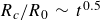 $R_{{c}}/R_{0}\,\sim \,t^{0.5}$
. Assuming that the vertical evolution of the droplet scales as
$R_{{c}}/R_{0}\,\sim \,t^{0.5}$
. Assuming that the vertical evolution of the droplet scales as $(R_{0}-{\unicode[Arial]{x0394}} h)/R_{0}\sim t^{-1}$
, we have
$(R_{0}-{\unicode[Arial]{x0394}} h)/R_{0}\sim t^{-1}$
, we have $((R_{0}-{\unicode[Arial]{x0394}} h)/{R_{0}})^{-0.5}\sim R_{{c}}/R_{0}$
. Substituting
$((R_{0}-{\unicode[Arial]{x0394}} h)/{R_{0}})^{-0.5}\sim R_{{c}}/R_{0}$
. Substituting $f=(s_{{p}}-w_{{p}})/s_{{p}}$
into (2.8) yields
$f=(s_{{p}}-w_{{p}})/s_{{p}}$
into (2.8) yields
 \begin{equation} \begin{array}{c} F_{\textit{capillary}}\sim \frac{\gamma \cos \left({\unicode[Arial]{x03B8}} _{{p}}\right){R}_{0}^{4}\left( 1-1.5f\right) }{{s}_{{p}}^{2}\left(R_{0}-{\unicode[Arial]{x0394}} h\right)}.\end{array} \end{equation}
In addition, the viscous force $F_{\textit{viscous}}$
during the droplet evolution can be scaled as
$F_{\textit{viscous}}$
during the droplet evolution can be scaled as
 , related to the reference velocity gradient
 (Delbos, Lorenceau & Pitois Reference Delbos, Lorenceau and Pitois2010). To facilitate the analysis, we only consider the forces on the symmetry plane of the droplet. In accordance with Newton’s second law, we can establish the equation of motion:
 \begin{equation} \begin{array}{c} m^{{*}}\frac{{\rm d}^{2}{\unicode[Arial]{x0394}} h}{{\rm d}t^{2}}\,=\frac{\gamma \cos \left({\unicode[Arial]{x03B8}} _{{p}}\right){R}_{0}^{4}\left( 1-1.5f\right) }{{s}_{{p}}^{2}\left(R_{0}-{\unicode[Arial]{x0394}} h\right)}-\frac{\mu _{l}}{R_{0}}\frac{{\rm d}{\unicode[Arial]{x0394}} {h}}{{\rm d}t}.\end{array} \end{equation}
Here $m^{{*}}$
is the effective mass on the two-dimensional plane with a dimension of
$m^{{*}}$
is the effective mass on the two-dimensional plane with a dimension of ${kg}\,{m}^{-2}$
, scaled as
${kg}\,{m}^{-2}$
, scaled as $m^{{*}}\,\sim \,\rho _{l}R_{0}$
. Normalising (2.10) using
$m^{{*}}\,\sim \,\rho _{l}R_{0}$
. Normalising (2.10) using ${\unicode[Arial]{x0394}} h^{{*}}={\unicode[Arial]{x0394}} h/R_{0}$
and
${\unicode[Arial]{x0394}} h^{{*}}={\unicode[Arial]{x0394}} h/R_{0}$
and $T^{{*}}$
, the equation becomes
$T^{{*}}$
, the equation becomes
 \begin{equation} \begin{array}{c} \frac{{\rm d}^{2}{\unicode[Arial]{x0394}} h^{{*}}}{{\rm d}T ^{*2}}=\frac{\cos \left(\theta _{{p}}\right){R}_{0}^{2}\left( 1-1.5f\right) }{{s}_{{p}}^{2}(1-{\unicode[Arial]{x0394}} h^{{*}})}-{Oh}\frac{{\rm d}{\unicode[Arial]{x0394}} h^{{*}}}{{\rm d}T^{{*}}}, \end{array} \end{equation}
where the Ohnesorge number is ${Oh }=\mu _{{l}}/\sqrt{\gamma \rho _{{l}}R_{0}}$
. By substituting the initial conditions, i.e.
${Oh }=\mu _{{l}}/\sqrt{\gamma \rho _{{l}}R_{0}}$
. By substituting the initial conditions, i.e. ${\unicode[Arial]{x0394}} h^{{*}}(0)=0$
and
${\unicode[Arial]{x0394}} h^{{*}}(0)=0$
and
 , the transient evolution of ${\unicode[Arial]{x0394}} h^{{*}}$
can be derived. It is noteworthy that in the above governing equation, a fitting parameter
${\unicode[Arial]{x0394}} h^{{*}}$
can be derived. It is noteworthy that in the above governing equation, a fitting parameter $\alpha =0.56$
is introduced to balance the effects of capillary and viscous forces. This parameter is determined by fitting the analytical model to simulation results for the maximum penetration depth across a range of cases. Its value may vary with different combinations of surface tension and viscosity. All other force terms are derived from realistic forcing balance. Thus, (2.11) can be directly applied to droplets of various sizes and different surface geometries. It should be clarified that the above model is only applicable to the penetration process after droplet impact on micropillar surfaces. For the rebound process, the direction of the viscous force changes, rendering this equation inapplicable. However, considering that the main objective here is to identify the relationship between the maximum droplet penetration depth and the parameters We and
$\alpha =0.56$
is introduced to balance the effects of capillary and viscous forces. This parameter is determined by fitting the analytical model to simulation results for the maximum penetration depth across a range of cases. Its value may vary with different combinations of surface tension and viscosity. All other force terms are derived from realistic forcing balance. Thus, (2.11) can be directly applied to droplets of various sizes and different surface geometries. It should be clarified that the above model is only applicable to the penetration process after droplet impact on micropillar surfaces. For the rebound process, the direction of the viscous force changes, rendering this equation inapplicable. However, considering that the main objective here is to identify the relationship between the maximum droplet penetration depth and the parameters We and $f$
, analysing the penetration process is sufficient.
$f$
, analysing the penetration process is sufficient.
During droplet impact, when the penetration depth exceeds the pillar height ( ${{\unicode[Arial]{x0394}} h}_{max}^{{*}}\gt H^{*}$
), the droplet exhibits a Wenzel state due to the hydrophilicity of the substrate; otherwise, the droplet remains in the Cassie state (
${{\unicode[Arial]{x0394}} h}_{max}^{{*}}\gt H^{*}$
), the droplet exhibits a Wenzel state due to the hydrophilicity of the substrate; otherwise, the droplet remains in the Cassie state ( ${{\unicode[Arial]{x0394}} h}_{max}^{{*}}\lt H^{*}$
). Therefore,
${{\unicode[Arial]{x0394}} h}_{max}^{{*}}\lt H^{*}$
). Therefore, ${{\unicode[Arial]{x0394}} h}_{max}^{{*}}$
can be used as a criterion for determining the bouncing outcomes of the impacting droplet. In the current study the capillary number
${{\unicode[Arial]{x0394}} h}_{max}^{{*}}$
can be used as a criterion for determining the bouncing outcomes of the impacting droplet. In the current study the capillary number ${Ca }=\mu _{l}V_{0}/\gamma$
, which represents the ratio of viscous force to surface tension, is at least one order of magnitude smaller than
${Ca }=\mu _{l}V_{0}/\gamma$
, which represents the ratio of viscous force to surface tension, is at least one order of magnitude smaller than $10^{-1}$
. As a result, the viscous term in (2.11) can be safely neglected. By implementing
$10^{-1}$
. As a result, the viscous term in (2.11) can be safely neglected. By implementing
 , the equation can thus be simplified as
 \begin{equation} \begin{array}{c} V\frac{{\rm d}V}{{\rm d}h^{{*}}}=\frac{\cos \left(\theta _{{p}}\right){R}_{0}^{2}\left( 1-1.5f\right) }{{s}_{{p}}^{2}(1-{\unicode[Arial]{x0394}} h^{{*}})},\end{array} \end{equation}
integrating both sides we obtain
 \begin{equation} \int V{\rm d}V=\int \frac{\cos \left(\theta _{{p}}\right){R}_{0}^{2}\left( 1-1.5f\right) }{{s}_{{p}}^{2}(1-{\unicode[Arial]{x0394}} h^{{*}})}{\rm d}h^{{*}}, \end{equation}
and applying the initial conditions, we have
 \begin{equation} \begin{array}{c} \frac{1}{2}V^{2}=-\frac{\cos \left(\theta _{{p}}\right){R}_{0}^{2}\left( 1-1.5f\right) }{{s}_{{p}}^{2}}\ln \left(1-{\unicode[Arial]{x0394}} h^{{*}}\right)+\frac{1}{2}{V}_{0}^{2}, \end{array} \end{equation}
considering that ${\unicode[Arial]{x0394}} h^{{*}}$
reaches its maximum value when
${\unicode[Arial]{x0394}} h^{{*}}$
reaches its maximum value when $\,V=0$
,
$\,V=0$
, ${{\unicode[Arial]{x0394}} h}_{max}^{*}$
can be predicted as
${{\unicode[Arial]{x0394}} h}_{max}^{*}$
can be predicted as
 \begin{equation} \begin{array}{c} {{\unicode[Arial]{x0394}} h}_{max}^{*}=1-\exp \left\{\frac{\alpha ^{2}{s}_{{p}}^{2}{\textit{We}}}{2{R}_{0}^{2}\cos \left(\theta _{{p}}\right)\left( 1-1.5f\right) }\right\}.\end{array} \end{equation}
Equation (2.15) can be used to determine the droplet impact outcomes under different impact conditions and surface geometries. It should be noted that the proposed model for predicting the maximum penetration depth covers a wide range of operating parameters, including droplet radius, impact velocity and micropillar geometry, and thus, requires extensive validation to demonstrate its reliability. In addition, several quantitative aspects of droplet dynamics remain to be explored, such as the dynamic evolution of the meniscus within micropillar arrays, the wetting state on hydrophilic substrates and the energy evolution of the droplet. It would be challenging and costly for experiments to provide well-resolved quantitative data of the required transient interfacial dynamics. On the other hand, the lattice Boltzmann simulations allow a systematic study of the dynamics process of droplet impact on heterogeneous wettability surfaces while providing quantitative data to validate the proposed model, as will be demonstrated in the following section.
3. Results and discussion
3.1. Droplet wetting and bouncing behaviours
Figure 4 illustrates the transient evolution of the droplet after impact at We = 12. Four cases were examined to explore the effects of $H^{*}\,$
and
$H^{*}\,$
and $f$
. In contrast to the dynamics of droplet impact on homogeneous wettability surfaces, four distinctly different impact outcomes were observed. For the case with the lowest pillar height and largest opening fraction (panel (a),
$f$
. In contrast to the dynamics of droplet impact on homogeneous wettability surfaces, four distinctly different impact outcomes were observed. For the case with the lowest pillar height and largest opening fraction (panel (a), $\,H^{*}=0.08,f=0.56$
), part of the liquid penetrates the micropillar array and contacts the substrate directly during droplet spreading (as shown in
$\,H^{*}=0.08,f=0.56$
), part of the liquid penetrates the micropillar array and contacts the substrate directly during droplet spreading (as shown in $T^{*}=t/\,t_{\sigma }=\,$
0.25 and 0.75). Subsequently, the droplet fully penetrates the pillars and reaches a complete Wenzel state (
$T^{*}=t/\,t_{\sigma }=\,$
0.25 and 0.75). Subsequently, the droplet fully penetrates the pillars and reaches a complete Wenzel state ( $T^{*}=1.25$
of panel a). Due to the hydrophilicity of the substrate, droplet rebound is suppressed and the droplet demonstrates a complete wetting morphology. For the case with a similar pillar height but smaller opening fraction (panel (b),
$T^{*}=1.25$
of panel a). Due to the hydrophilicity of the substrate, droplet rebound is suppressed and the droplet demonstrates a complete wetting morphology. For the case with a similar pillar height but smaller opening fraction (panel (b), $\,H^{*}=0.08,f=0.33$
), a similar liquid penetration and adhesion process is observed (see
$\,H^{*}=0.08,f=0.33$
), a similar liquid penetration and adhesion process is observed (see $T^{*}=0.75$
and 1.25 in panel b). Then, due to the droplet rebound, the Wenzel state is disrupted, and the main part of the droplet bounces off the surface. However, a small portion of the droplet remains adhered to the hydrophilic substrate, resulting in a partial wetting morphology.
$T^{*}=0.75$
and 1.25 in panel b). Then, due to the droplet rebound, the Wenzel state is disrupted, and the main part of the droplet bounces off the surface. However, a small portion of the droplet remains adhered to the hydrophilic substrate, resulting in a partial wetting morphology.
The wetting and bouncing behaviours of droplets impacting mixed-wettability pillared surfaces with varying We, pillar height $(H^{{*}})$
and opening fractions (f).
$(H^{{*}})$
and opening fractions (f).

Figure 4. Long description
The illustration shows four different scenarios of droplet impact behaviors on surfaces with varying wettability and pillar configurations. Each scenario is labeled with specific parameters such as We, f, and H*. The first scenario, labeled as complete wetting, shows a droplet spreading out and wetting the surface completely. The second scenario, labeled as partial wetting, shows a droplet partially wetting the surface. The third scenario, labeled as complete bouncing, shows a droplet bouncing off the surface without wetting it. The fourth scenario, labeled as pancake bouncing, shows a droplet flattening out and then bouncing off the surface. Each scenario is depicted with a series of images showing the droplet at different stages of impact.
As indicated in panels (a) and (b) of figure 4, Wenzel state droplets exhibit wetting morphologies due to the hydrophilicity of the substrate. On the other hand, Cassie state droplets show evolution similar to that observed during impingement on a superhydrophobic pillared surface. For example, for the case with a smaller opening fraction (panel (c), $H^{*}=0.05\,,f=0.2$
), the penetration of the liquid is suspended due to the increasing capillary resistance, and the droplet rebound follows a typical complete rebound morphology. For the case with the highest pillar height and largest opening fraction (panel (d),
$H^{*}=0.05\,,f=0.2$
), the penetration of the liquid is suspended due to the increasing capillary resistance, and the droplet rebound follows a typical complete rebound morphology. For the case with the highest pillar height and largest opening fraction (panel (d), $H^{*}=0.33\,,f=0.56$
), liquid first penetrates into the micropillar gaps and then retracts before it touches the substrate, the droplet presents a typical pancake bouncing morphology as shown in figure 2.
$H^{*}=0.33\,,f=0.56$
), liquid first penetrates into the micropillar gaps and then retracts before it touches the substrate, the droplet presents a typical pancake bouncing morphology as shown in figure 2.
We first focus on the rebound dynamics of droplets in the Cassie state. Figure 5(a) depicts the dynamics of a bouncing droplet at varying We ( $H^{*}=0.5\,,f=0.56$
). The droplet is coloured by the normalised pressure (
$H^{*}=0.5\,,f=0.56$
). The droplet is coloured by the normalised pressure ( $P/(2\gamma /R_{0})$
) with velocity vectors (coloured by velocity magnitude) superimposed. At the penetration stage (
$P/(2\gamma /R_{0})$
) with velocity vectors (coloured by velocity magnitude) superimposed. At the penetration stage ( $T^{*}=\,0.2$
), the droplet’s bottom penetrates into the pillar gaps, during which the dynamics is governed by the competition between inertial effects and capillary force. For cases with higher We, a higher pressure is observed in the penetrated liquid. As anticipated from a previous study (Moevius et al. Reference Moevius, Liu, Wang and Yeomans2014), the KE is converted into SE; therefore, a higher We increases the distance between the droplet’s bottom surface (P
1) and pillars’ top surface (denoted as h in the following). At
$T^{*}=\,0.2$
), the droplet’s bottom penetrates into the pillar gaps, during which the dynamics is governed by the competition between inertial effects and capillary force. For cases with higher We, a higher pressure is observed in the penetrated liquid. As anticipated from a previous study (Moevius et al. Reference Moevius, Liu, Wang and Yeomans2014), the KE is converted into SE; therefore, a higher We increases the distance between the droplet’s bottom surface (P
1) and pillars’ top surface (denoted as h in the following). At $T^{{*}}=0.4$
, the mother droplet above the pillar surface further spreads while the penetrated liquid begins to retract (as demonstrated by the velocity vector components), during which SE is transferred back to KE. By
$T^{{*}}=0.4$
, the mother droplet above the pillar surface further spreads while the penetrated liquid begins to retract (as demonstrated by the velocity vector components), during which SE is transferred back to KE. By $T^{{*}}=\,0.86$
, the droplet fully retracts and bounces off from the plate. A higher We leads to a larger amount of transferred KE, and therefore, pancake bouncing morphology is clearly observed for the large We cases (e.g. We = 16). The dynamics of droplet penetration into the pillar gaps is shown in figure 5(b) using two-dimensional slices along the symmetry plane. It can be seen that, for all cases in figure 5(a), the three-phase contact line moves below the top of the pillars during the penetration stage. Owing to the superhydrophobic wettability of the pillar surfaces, the liquid penetrating into the pillar gaps forms curved menisci, which provide one of the main contributions to the capillary resistance force.
$T^{{*}}=\,0.86$
, the droplet fully retracts and bounces off from the plate. A higher We leads to a larger amount of transferred KE, and therefore, pancake bouncing morphology is clearly observed for the large We cases (e.g. We = 16). The dynamics of droplet penetration into the pillar gaps is shown in figure 5(b) using two-dimensional slices along the symmetry plane. It can be seen that, for all cases in figure 5(a), the three-phase contact line moves below the top of the pillars during the penetration stage. Owing to the superhydrophobic wettability of the pillar surfaces, the liquid penetrating into the pillar gaps forms curved menisci, which provide one of the main contributions to the capillary resistance force.
(a) The dynamic evolution of droplet impact on mixed-wettability pillared surfaces ( $H^{{*}}=0.5\,,f=0.56$
) with varying We. (b) Two-dimensional slices along the symmetry plane showing the evolution of the droplet profile (highlighted by coloured lines) at
$H^{{*}}=0.5\,,f=0.56$
) with varying We. (b) Two-dimensional slices along the symmetry plane showing the evolution of the droplet profile (highlighted by coloured lines) at $T^{*}=0.1$
, 0.2 and 0.4 for cases in figure 5(a).
$T^{*}=0.1$
, 0.2 and 0.4 for cases in figure 5(a).

Figure 5. Long description
The image consists of two main parts labeled (a) and (b). Part (a) displays the dynamic evolution of droplet impact on mixed-wettability pillared surfaces with varying Weber numbers. It includes three rows, each representing different stages of droplet impact: penetrating and spreading, spreading and draining, and retracting and rebounding. Each row contains three columns showing different Weber numbers: 8, 12, and 16. The columns depict pressure factor and velocity magnitude using color gradients and arrows to indicate direction and magnitude. Part (b) shows two-dimensional slices along the symmetry plane, illustrating the evolution of the droplet profile at different time intervals (T* = 0.1, 0.2, and 0.4) for cases in figure 5(a). The profiles are highlighted by colored lines (red, blue, and green) corresponding to different Weber numbers (8, 12, and 16). The image provides a detailed visual representation of how droplets behave upon impact with substrates under different conditions.
The transient evolution of the normalised (a) droplet radius variation ( ${\unicode[Arial]{x0394}} R^{{*}}$
) and (b) droplet penetration depth within the pillars (
${\unicode[Arial]{x0394}} R^{{*}}$
) and (b) droplet penetration depth within the pillars ( $h^{{*}}$
) for cases with varying We and opening fractions (
$h^{{*}}$
) for cases with varying We and opening fractions ( $f$
). The inset figure in panel (b) illustrates the instant of droplet bouncing off the surface.
$f$
). The inset figure in panel (b) illustrates the instant of droplet bouncing off the surface.

Figure 6. Long description
The image contains two line graphs. The first graph (a) shows the transient evolution of the normalized droplet radius variation (•R*) over time (T*) for different Weber numbers (We) and opening fractions (f). The second graph (b) illustrates the droplet penetration depth (h*) within the pillars over time (T*) for the same varying conditions. The inset in panel (b) highlights the moment when the droplet bounces off the surface. The graphs compare cases with We values of 23, 12, and 8, and opening fractions of 0.43 and 0.56. The red line represents We = 23 and f = 0.43, the light blue dashed line represents We = 12 and f = 0.56, the blue dashed line represents We = 12 and f = 0.43, and the solid blue line represents We = 8 and f = 0.56. The graphs show how these parameters influence the droplet's behavior upon impact with the superhydrophobic surface.
To further investigate the influence of micropillar geometry and impact conditions on the transient dynamics of a Cassie state droplet, figure 6 presents the time evolution of the normalised droplet radius variation ( ${\unicode[Arial]{x0394}} R^{{*}}=(R-R_{0})/R_{0}$
, where R denotes the maximum horizontal displacement of the droplet) and penetration depth (
${\unicode[Arial]{x0394}} R^{{*}}=(R-R_{0})/R_{0}$
, where R denotes the maximum horizontal displacement of the droplet) and penetration depth ( ${\unicode[Arial]{x0394}} h^{{*}}=(0-\,h)/R_{0}$
) for different impact We and
${\unicode[Arial]{x0394}} h^{{*}}=(0-\,h)/R_{0}$
) for different impact We and $\,f$
. As demonstrated in figure 6(a), in all cases,
$\,f$
. As demonstrated in figure 6(a), in all cases, ${\unicode[Arial]{x0394}} R^{{*}}\,$
increases initially and then decreases as the droplet retracts. Similar to previous experimental observations for droplet impact on a non-wetting surface (Illias et al. Reference Illias2021; Gao et al. Reference Gao2024), the maximum spreading time is around
${\unicode[Arial]{x0394}} R^{{*}}\,$
increases initially and then decreases as the droplet retracts. Similar to previous experimental observations for droplet impact on a non-wetting surface (Illias et al. Reference Illias2021; Gao et al. Reference Gao2024), the maximum spreading time is around $\,t_{max}/t_{\sigma }\sim \,0.8$
and independent of We. The maximum spreading diameter of the droplet increases as We increases. Figure 6(b) shows the evolution of
$\,t_{max}/t_{\sigma }\sim \,0.8$
and independent of We. The maximum spreading diameter of the droplet increases as We increases. Figure 6(b) shows the evolution of $h^{*}$
, in agreement with the qualitative results shown in figures 4 and 5. Increasing both We and
$h^{*}$
, in agreement with the qualitative results shown in figures 4 and 5. Increasing both We and $\,f\,$
enhances the penetration of the liquid into the pillars, owing to the dominance of dynamic forcing over capillary force in the vertical direction. After reaching the maximum penetration depth, the penetrated liquid drains from the pillar gaps. For the cases with higher We, owing to the larger SE storage, the droplet directly rebounds from the plate (points (1, 2, 3) in the inset of figure 6
b) and exhibits the pancake bouncing morphology with contact time
$\,f\,$
enhances the penetration of the liquid into the pillars, owing to the dominance of dynamic forcing over capillary force in the vertical direction. After reaching the maximum penetration depth, the penetrated liquid drains from the pillar gaps. For the cases with higher We, owing to the larger SE storage, the droplet directly rebounds from the plate (points (1, 2, 3) in the inset of figure 6
b) and exhibits the pancake bouncing morphology with contact time $t_{c}/\,t_{\sigma }\lt \,1$
. For the cases with lower We (e.g. We = 8), the droplet remains in contact with the plate and follows a complete rebound morphology, which is similar to the transient evolution shown in figure 5.
$t_{c}/\,t_{\sigma }\lt \,1$
. For the cases with lower We (e.g. We = 8), the droplet remains in contact with the plate and follows a complete rebound morphology, which is similar to the transient evolution shown in figure 5.
(a) Maximum spreading factors ( $\beta _{max}$
) and (b) liquid–solid contact time (
$\beta _{max}$
) and (b) liquid–solid contact time ( $\,t_{c}/t_{\sigma }$
) of droplets impacting mixed-wettability pillared surfaces with varying Weber numbers and opening fractions.
$\,t_{c}/t_{\sigma }$
) of droplets impacting mixed-wettability pillared surfaces with varying Weber numbers and opening fractions.

Figure 7. Long description
The image contains two separate graphs labeled (a) and (b). Graph (a) is a plot of the maximum spreading factors (beta max) against the Weber number (We) on a logarithmic scale. It includes three datasets represented by different symbols: triangles for f equals 0.2, squares for f equals 0.43, and circles for f equals 0.56. The graph shows a solid line and a dashed line, which are theoretical models. The data points indicate that as the Weber number increases, the maximum spreading factor also increases, with different trends for each opening fraction. Graph (b) is a plot of the liquid-solid contact time (t_c/t_sigma) against the Weber number (We) on a linear scale. It includes the same three datasets represented by the same symbols. The graph shows that the contact time remains relatively constant for different opening fractions as the Weber number increases. The graphs illustrate the relationship between droplet impact dynamics and surface configurations.
In the following, we focus on the bouncing droplets and quantitatively examine two key parameters during impact: the maximum spreading diameter and the contact time, which are of particular interest for characterising droplet dynamics. In figure 7(a) we recorded the droplet maximum spreading diameters and compared our simulation results with the scaling model proposed by Wörner (Reference Wörner2023), which can give an accurate prediction of the maximum spreading coefficient $\beta _{max}$
(ratio of the maximum wetting radius to the initial radius) for a wide range of We, where (Wörner Reference Wörner2023)
$\beta _{max}$
(ratio of the maximum wetting radius to the initial radius) for a wide range of We, where (Wörner Reference Wörner2023)
 \begin{equation} \begin{array}{c} \beta _{\textit{max}}=\sqrt{\frac{2\left(Q_{\beta }+a\cos \theta _{{p}}\right)+2\sqrt{\left(Q_{\beta }+a\cos \theta _{{p}}\right)^{2}+4aQ_{\beta }\left(1-\cos \theta _{{p}}\right)}}{1-\cos \theta _{{p}}}}, \end{array} \end{equation}
where $\,a\,$
is a fitting parameter and
$\,a\,$
is a fitting parameter and $Q_{\beta }\,$
is given as
$Q_{\beta }\,$
is given as
 \begin{align} Q_{\beta }&=1-a+\frac{{\textit{We}}}{12}-f_{w}w_{{\infty }},\notag\\ w_{{\infty }}&=1-\left(\frac{1}{3}\sqrt{0.25\left(2+\theta _{{p}}\right)\left(1-\theta _{{p}}\right)^{2}+\frac{{\textit{We}}}{12}}\right),\notag\\ f_{w}&=\frac{{\textit{WeRe}}^{-2/5}}{1.2-\cos \theta _{{p}}+{\textit{WeRe}}^{-2/5}}. \end{align}
The solid line in figure 7(a) represents the experimental fitting parameter $a=0.75$
in Wörner’s work (Reference Wörner2023) and the dashed line corresponds to
$a=0.75$
in Wörner’s work (Reference Wörner2023) and the dashed line corresponds to $a=0.6$
, providing the best fit to our simulation results. It can be found that, at lower We (i.e.
$a=0.6$
, providing the best fit to our simulation results. It can be found that, at lower We (i.e. ${We }\lt 10^{1}$
), the opening fraction
${We }\lt 10^{1}$
), the opening fraction $f$
has negligible influence on
$f$
has negligible influence on $\beta _{max}$
owing to the limited penetrated liquid in the micropillar gaps. At higher We (i.e.
$\beta _{max}$
owing to the limited penetrated liquid in the micropillar gaps. At higher We (i.e. ${\textit{We}}\gt 10^{1}$
), for cases with a large
${\textit{We}}\gt 10^{1}$
), for cases with a large $\,f$
, liquid penetration into the micropillar array results in a nearly constant
$\,f$
, liquid penetration into the micropillar array results in a nearly constant $\,\beta _{max}\,$
of approximately 1.7. This saturation of the maximum spreading radius due to volume loss through penetration is similar to the observation reported for droplet impacts on superhydrophobic mesh arrays (Kumar et al. Reference Kumar2018) and the quantitative results shown in figure 7. For the cases with a smaller
$\,\beta _{max}\,$
of approximately 1.7. This saturation of the maximum spreading radius due to volume loss through penetration is similar to the observation reported for droplet impacts on superhydrophobic mesh arrays (Kumar et al. Reference Kumar2018) and the quantitative results shown in figure 7. For the cases with a smaller $\,f$
,
$\,f$
, $\beta _{max}\,$
aligns closely with the scaling prediction because of the small amount of liquid penetration in the pillar gaps.
$\beta _{max}\,$
aligns closely with the scaling prediction because of the small amount of liquid penetration in the pillar gaps.
Figure 7(b) illustrates $\,t_{c}/\,t_{\sigma }$
as a function of We for cases of the Cassie state droplet. It can be seen that the criterion determining the droplet rebound morphology mainly depends on the We. That is, for a lower impact We (i.e. We < 12), almost all cases demonstrate complete rebound with
$\,t_{c}/\,t_{\sigma }$
as a function of We for cases of the Cassie state droplet. It can be seen that the criterion determining the droplet rebound morphology mainly depends on the We. That is, for a lower impact We (i.e. We < 12), almost all cases demonstrate complete rebound with $\,t_{c}/\,t_{\sigma }\approx 2.2\,$
(solid line in figure 7
b), consistent with Rayleigh’s theory (Ernest, August & Strutt Reference Ernest, August and Strutt1879). For higher impact We (i.e. We > 12), most cases demonstrate pancake bouncing morphologies with a much shorter
$\,t_{c}/\,t_{\sigma }\approx 2.2\,$
(solid line in figure 7
b), consistent with Rayleigh’s theory (Ernest, August & Strutt Reference Ernest, August and Strutt1879). For higher impact We (i.e. We > 12), most cases demonstrate pancake bouncing morphologies with a much shorter $\,t_{c}/\,t_{\sigma }\approx 0.56$
(dashed line in figure 7
b), which aligns with previous experimentally measured values. Meanwhile, it can also be observed that a smaller
$\,t_{c}/\,t_{\sigma }\approx 0.56$
(dashed line in figure 7
b), which aligns with previous experimentally measured values. Meanwhile, it can also be observed that a smaller $f$
leads to a higher We for the pancake bouncing regime, as a higher dynamic force is needed to achieve penetration.
$f$
leads to a higher We for the pancake bouncing regime, as a higher dynamic force is needed to achieve penetration.
Simulation snapshots (taken along the symmetry plane of the droplet) of droplet impact on surfaces with different micropillar geometries at We = 16. Velocity vectors are coloured according to velocity magnitude.

Figure 8. Long description
The image contains three sets of simulation snapshots showing droplet impact on surfaces with different micropillar geometries at a Weber number of 16. Each set includes four snapshots taken along the symmetry plane of the droplet at different time points. The snapshots are labeled as complete wetting, partial wetting, and partial wetting with different parameters. Velocity vectors are colored according to velocity magnitude, ranging from blue to red. The snapshots illustrate the dynamic behavior of droplets upon impact with substrates, highlighting different impact outcomes such as adhesion, rebound, or splashing. The image provides a visual representation of the fundamental physical understanding of droplet impact dynamics, which is essential for various industrial and engineering applications.
We then focus on the wetting dynamics of droplets in the Wenzel state. Figure 8 shows the evolution of wetting droplets for cases with different micropillar geometries at We = 16. It can be seen that, for all cases, wetting of the hydrophilic substrate by the penetrated liquid occurs during the impact stage. For the complete wetting droplet (panel a), no fragmentation or separation of the main droplet is observed during retraction and rebound stages. Meanwhile, during the retraction stage, the liquid on the substrate retracts more slowly than the mother droplet due to the pinning effect. In contrast, for partially wetted droplets (panels b and c), either a higher pillar density (smaller $\,{s}_{{p}}$
) increases the capillary pressure (
$\,{s}_{{p}}$
) increases the capillary pressure ( $\sim \,2\gamma \cos (\theta _{{p}})/(s_{{p}}-w_{{p}})$
) or a greater pillar height (
$\sim \,2\gamma \cos (\theta _{{p}})/(s_{{p}}-w_{{p}})$
) or a greater pillar height ( $h_{{p}}$
) increases the risk of liquid bridge breakup between the mother droplet and the pinned liquid at the base. As a result, splitting of the pinned liquid from the mother droplet is observed during the retraction stage, and rebound of the mother droplet occurs at the end of the simulation. In this work we introduce an effective contact angle (
$h_{{p}}$
) increases the risk of liquid bridge breakup between the mother droplet and the pinned liquid at the base. As a result, splitting of the pinned liquid from the mother droplet is observed during the retraction stage, and rebound of the mother droplet occurs at the end of the simulation. In this work we introduce an effective contact angle ( $\theta _{{e}ff}$
) to characterise the competition between pinning (due to the hydrophilic substrate) and depinning (due to the superhydrophobic micropillars) effects. The effective contact angle is constructed using the full form of the Cassie equation (Milne, Amirfazli & Baxter Reference Milne, Amirfazli and Baxter2012), i.e.
$\theta _{{e}ff}$
) to characterise the competition between pinning (due to the hydrophilic substrate) and depinning (due to the superhydrophobic micropillars) effects. The effective contact angle is constructed using the full form of the Cassie equation (Milne, Amirfazli & Baxter Reference Milne, Amirfazli and Baxter2012), i.e.
 \begin{equation} \cos \left(\theta _{\textit{eff}}\right)=\sum _{n}f_{s,n}\cos \left(\theta _{n}\right)\!, \end{equation}
where the summation covers n interfaces under the droplet and $f_{s,n}$
denotes the surface fraction of each component. When the droplet contacts the substrate, the equation reduces to
$f_{s,n}$
denotes the surface fraction of each component. When the droplet contacts the substrate, the equation reduces to
 \begin{equation} \begin{array}{c} \cos \left(\theta _{\textit{eff}}\right)=\left(1-f_{s}\right)\cos \left(\theta _{{s}}\right)+f_{s}\cos \left(\theta _{{p}}\right)\!,\end{array} \end{equation}
and the solid fraction is given by
 \begin{equation} \begin{array}{c} f_{s}=\frac{\pi \left(\left(1-f\right)R_{0}\right)^{2}+4\left(1-f\right)R_{0}h_{{p}}}{\pi {R}_{0}^{2}}. \end{array} \end{equation}
It should be noted that (3.4) is only applicable for characterising the Wenzel state. For droplets in the Cassie state, the effective contact angle can be expressed as $\cos (\theta _{\textit{eff}})=f_{s}(\cos (\theta _{p})+1)-1$
. By comparing the qualitative results in figure 8 with
$\cos (\theta _{\textit{eff}})=f_{s}(\cos (\theta _{p})+1)-1$
. By comparing the qualitative results in figure 8 with $\theta _{\textit{eff}}$
calculated from (3.5), it is found that, as expected, a smaller
$\theta _{\textit{eff}}$
calculated from (3.5), it is found that, as expected, a smaller $\theta _{\textit{eff}}$
promotes pinning, while a larger
$\theta _{\textit{eff}}$
promotes pinning, while a larger $\theta _{\textit{eff}}$
facilitates rebound. As a result, the amount of liquid remaining on the surface after rebound is minimised for cases with larger
$\theta _{\textit{eff}}$
facilitates rebound. As a result, the amount of liquid remaining on the surface after rebound is minimised for cases with larger $\theta _{\textit{eff}}$
. It should be noted that we chose
$\theta _{\textit{eff}}$
. It should be noted that we chose $R_{0}$
as the reference length scale in (3.5), and the expansion effect of droplets for various We has been ignored. Therefore,
$R_{0}$
as the reference length scale in (3.5), and the expansion effect of droplets for various We has been ignored. Therefore, $\theta _{\textit{eff}}$
is only applicable for evaluating the pinning and depinning effects at a fixed impact We.
$\theta _{\textit{eff}}$
is only applicable for evaluating the pinning and depinning effects at a fixed impact We.
We now consider the effect of different impact We on the dynamics of Wenzel state droplets. Figure 9 illustrates the evolution of the normalised droplet radius ${\unicode[Arial]{x0394}} R^{*}$
(left axis) for both wetting droplets (dashed lines) and bouncing droplets (solid lines). It can be concluded that, for higher We (i.e. We = 12 and We = 16), the terminal droplet radius is larger for complete wetting cases than for rebound droplets, due to the pinning of liquid on the substrate that inhibits retraction (also demonstrated in figure 8). As expected, for lower impact We, the suppression of retraction caused by the pinning effect is less pronounced. We also plotted the transient evolution of the liquid–solid contact area (
${\unicode[Arial]{x0394}} R^{*}$
(left axis) for both wetting droplets (dashed lines) and bouncing droplets (solid lines). It can be concluded that, for higher We (i.e. We = 12 and We = 16), the terminal droplet radius is larger for complete wetting cases than for rebound droplets, due to the pinning of liquid on the substrate that inhibits retraction (also demonstrated in figure 8). As expected, for lower impact We, the suppression of retraction caused by the pinning effect is less pronounced. We also plotted the transient evolution of the liquid–solid contact area (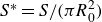 $S^{*}=S/(\pi\kern-1pt {R}_{0}^{2})$
, shown as filled patterns in figure 9
b) for wetting cases, complemented by qualitative snapshots (figures in dashed brackets) of the bottom surface contact area (blue patterns, coloured by velocity). As shown in the snapshots, a ring-shaped contact area with holes is initially formed, resulting from gas expulsion beneath the spreading film. As the penetrated liquid wets the surface, the contact area increases and reaches its maximum value. Both qualitative and quantitative results indicate that, similar to the case of droplets impacting hydrophilic surfaces, the maximum wetting area for fully wetted droplets also increases with increasing We and stabilises during the retraction process.
$S^{*}=S/(\pi\kern-1pt {R}_{0}^{2})$
, shown as filled patterns in figure 9
b) for wetting cases, complemented by qualitative snapshots (figures in dashed brackets) of the bottom surface contact area (blue patterns, coloured by velocity). As shown in the snapshots, a ring-shaped contact area with holes is initially formed, resulting from gas expulsion beneath the spreading film. As the penetrated liquid wets the surface, the contact area increases and reaches its maximum value. Both qualitative and quantitative results indicate that, similar to the case of droplets impacting hydrophilic surfaces, the maximum wetting area for fully wetted droplets also increases with increasing We and stabilises during the retraction process.
(a) The transient evolution of the normalised droplet radius variation (lines in the graph) and liquid–solid contact area (patterns in the graph), (b) the qualitative snapshots illustrating the liquid–solid contact area on the bottom surface.

Figure 9. Long description
The image contains two graphs and a series of qualitative snapshots illustrating droplet impact dynamics on solid surfaces. The first graph (a) shows the transient evolution of the normalized droplet radius variation and liquid-solid contact area for different Weber numbers (We = 8, 12, 16). The x-axis represents the normalized time (T*), and the y-axis represents the normalized droplet radius variation (•R*) and liquid-solid contact area (S'). The graph uses solid and dashed lines to differentiate between wetting and bouncing behaviors. The second part (b) presents qualitative snapshots illustrating the liquid-solid contact area on the bottom surface at different normalized times (T* = 0.53, 1.6, 2.4) for different Weber numbers (We = 8, 12, 16). Each row of snapshots corresponds to a specific Weber number and shows the normalized velocity within the droplet. The snapshots are color-coded to represent different values of normalized velocity.
In conclusion of the above findings, the wetting and bouncing behaviours of droplets on the heterogeneous wettability surfaces are directly governed by the penetration dynamics of liquid into the pillars. In following section, we validate the force balance analysis provided in § 2.4 over a wide range of surface geometrical parameters and impact conditions.
3.2. Droplet dynamic evolution
Figures 10(a) and 10(b) illustrate the evolution of ${\unicode[Arial]{x0394}} h^{{*}}$
for cases with different impact We at
${\unicode[Arial]{x0394}} h^{{*}}$
for cases with different impact We at $\,f=0.56\,$
(figure 10
a) and
$\,f=0.56\,$
(figure 10
a) and $\,f=0.43\,$
(figure 10
b), together with a comparison to the proposed model ((2.15), lines in figure). As shown in the figures, our proposed analytical model provides a good prediction of
$\,f=0.43\,$
(figure 10
b), together with a comparison to the proposed model ((2.15), lines in figure). As shown in the figures, our proposed analytical model provides a good prediction of ${\unicode[Arial]{x0394}} h^{{*}}$
during the penetration stage. In addition, it can be observed that
${\unicode[Arial]{x0394}} h^{{*}}$
during the penetration stage. In addition, it can be observed that ${\unicode[Arial]{x0394}} h^{{*}}$
increases almost linearly (slope = 1.0) with
${\unicode[Arial]{x0394}} h^{{*}}$
increases almost linearly (slope = 1.0) with $T^{{*}}$
for all cases during the early stage of penetration. This is because the droplet penetration is mainly governed by inertial effects at this stage. At the later stage of penetration, both viscous and capillary forces begin to act and resist further penetration, the penetrated portion eventually retracts after reaching the maximum penetration depth (
$T^{{*}}$
for all cases during the early stage of penetration. This is because the droplet penetration is mainly governed by inertial effects at this stage. At the later stage of penetration, both viscous and capillary forces begin to act and resist further penetration, the penetrated portion eventually retracts after reaching the maximum penetration depth ( ${{\unicode[Arial]{x0394}} h}_{max}^{*})$
. As expected, discrepancies between the analytical model and our lattice Boltzmann simulation results begin to emerge during the rebound phase (i.e. time instant after
${{\unicode[Arial]{x0394}} h}_{max}^{*})$
. As expected, discrepancies between the analytical model and our lattice Boltzmann simulation results begin to emerge during the rebound phase (i.e. time instant after ${{\unicode[Arial]{x0394}} h}_{max}^{*}$
).
${{\unicode[Arial]{x0394}} h}_{max}^{*}$
).
A quantitative comparison of the droplet penetration depth inside pillars under various We, with opening fractions of (a) f = 0.56 and (b) f = 0.43. Panel (c) presents a comparison between the simulation results and the analytical model of the maximum penetration depth, as determined by (2.15).

Figure 10. Long description
The image contains three graphs comparing droplet penetration depth under various conditions. Graphs (a) and (b) show the penetration depth inside pillars with opening fractions of 0.56 and 0.43, respectively. Each graph plots penetration depth (Delta h*) against a dimensionless time parameter (T*) for different Weber numbers (We = 23, 16, 12). The lines and symbols represent different Weber numbers and their corresponding data points. Graph (c) compares simulation results with an analytical model of the maximum penetration depth, plotting simulated penetration depth (Delta h*_Sim theory) against theoretical maximum penetration depth (Delta h*_max theory). The data points closely follow a diagonal line, indicating good agreement between the simulation and the model. All values are approximated.
A transition diagram of droplet impact outcomes under varying $We$
,
$We$
, ${{\unicode[Arial]{x0394}} h}_{max}^{*}-H^*$
in the vertical axis represents the critical value determined by (2.15).
${{\unicode[Arial]{x0394}} h}_{max}^{*}-H^*$
in the vertical axis represents the critical value determined by (2.15).

Figure 11. Long description
The image contains two graphs. The left graph is a scatter plot with different symbols representing various droplet impact outcomes: complete bouncing (red triangles), pancake bouncing (orange squares), and complete wetting/partial wetting (blue circles). The x-axis represents the Weber number (We), and the y-axis represents the normalized maximum height difference (•h*max - H*). The right graph is a heat map showing the ratio of spreading time to oscillation time (tσ/tc) as a function of We and •h*max - H*. The heat map uses a color gradient to indicate different values of tσ/tc. The scatter plot and heat map together illustrate how droplet impact outcomes vary with We and the critical value determined by (2.15).
Figure 10(c) compares the simulated maximum penetration depths (symbols) with the proposed model (line in the figure). It can be seen that our proposed model demonstrates good agreement with the simulation results over a wide range of ${\unicode[Arial]{x0394}} h^{{*}}$
. For most cases, the maximum error is less than 20 % (within the region between the dashed lines). It should be emphasised that the above analytical model is derived based on the competition between forces, and the size effects of both the micropillars and the droplet are taken into account. Therefore, the model is applicable to a wide range of micropillar surface structures, droplet sizes and impact conditions. This generality warrants further validation in future experimental and numerical studies.
${\unicode[Arial]{x0394}} h^{{*}}$
. For most cases, the maximum error is less than 20 % (within the region between the dashed lines). It should be emphasised that the above analytical model is derived based on the competition between forces, and the size effects of both the micropillars and the droplet are taken into account. Therefore, the model is applicable to a wide range of micropillar surface structures, droplet sizes and impact conditions. This generality warrants further validation in future experimental and numerical studies.
Figure 11 presents a transition diagram illustrating the impact outcomes of all cases explored in the current study. The vertical axis shows the criterion of the Cassie state and Wenzel state, which is determined by ${{\unicode[Arial]{x0394}} h}_{max}^{{*}}-H^{*}$
. For the Cassie state droplet with
${{\unicode[Arial]{x0394}} h}_{max}^{{*}}-H^{*}$
. For the Cassie state droplet with ${h}_{max}^{{*}}-H^{*}\lt 0$
and lower
${h}_{max}^{{*}}-H^{*}\lt 0$
and lower $We$
, the droplet undergoes complete rebound due to limited penetration of liquid in the pillars’ gap. As We increases, enhanced energy transfer between KE and SE promotes pancake bouncing. A dashed vertical line at We = 12 marks the empirical threshold between complete rebound and pancake bouncing, as suggested in previous studies (Liu et al. Reference Liu, Moevius, Xu, Qian, Yeomans and Wang2014; Wang et al. Reference Wang, Sohani, Yang, Lei, Chen, He and Luo2025) and supported by our current simulation results. It is worth noting that, near the regime boundary (We = 12 and
$We$
, the droplet undergoes complete rebound due to limited penetration of liquid in the pillars’ gap. As We increases, enhanced energy transfer between KE and SE promotes pancake bouncing. A dashed vertical line at We = 12 marks the empirical threshold between complete rebound and pancake bouncing, as suggested in previous studies (Liu et al. Reference Liu, Moevius, Xu, Qian, Yeomans and Wang2014; Wang et al. Reference Wang, Sohani, Yang, Lei, Chen, He and Luo2025) and supported by our current simulation results. It is worth noting that, near the regime boundary (We = 12 and $\,{{\unicode[Arial]{x0394}} h}_{max}^{{*}}-H^{*}\lt 0$
), we observed some overlap between pancake bouncing and complete rebound cases. This is because the critical We for the onset of pancake bouncing can vary with the micropillar geometry (as shown in figure 7
b). However, over a broader range of We outside the immediate boundary region, using We as the criterion to distinguish between pancake bouncing and complete rebound remains robust and effective. In addition, we plotted a contour map of
$\,{{\unicode[Arial]{x0394}} h}_{max}^{{*}}-H^{*}\lt 0$
), we observed some overlap between pancake bouncing and complete rebound cases. This is because the critical We for the onset of pancake bouncing can vary with the micropillar geometry (as shown in figure 7
b). However, over a broader range of We outside the immediate boundary region, using We as the criterion to distinguish between pancake bouncing and complete rebound remains robust and effective. In addition, we plotted a contour map of $\,t_{c}/\,t_{\sigma }$
for all Cassie state droplets in the inset of figure 11 (dashed box). Consistent with the results in figure 7(b), as We increases,
$\,t_{c}/\,t_{\sigma }$
for all Cassie state droplets in the inset of figure 11 (dashed box). Consistent with the results in figure 7(b), as We increases, $\,t_{c}/\,t_{\sigma }$
decreases due to the occurrence of pancake bouncing. In contrast, the value of
$\,t_{c}/\,t_{\sigma }$
decreases due to the occurrence of pancake bouncing. In contrast, the value of ${{\unicode[Arial]{x0394}} h}_{max}^{{*}}-H^{*}$
has little effect on the rebound time of the droplet.
${{\unicode[Arial]{x0394}} h}_{max}^{{*}}-H^{*}$
has little effect on the rebound time of the droplet.
For cases where ${{\unicode[Arial]{x0394}} h}_{max}^{{*}}-H^{*}\gt 0$
, the droplet exhibits a Wenzel state with the penetrated liquid wetting the hydrophilic surface. For higher We, partial wetting is observed when
${{\unicode[Arial]{x0394}} h}_{max}^{{*}}-H^{*}\gt 0$
, the droplet exhibits a Wenzel state with the penetrated liquid wetting the hydrophilic surface. For higher We, partial wetting is observed when ${{\unicode[Arial]{x0394}} h}_{max}^{{*}}-H^{*}\approx 0$
. As analysed in figure 8, this is due to the fact that a small penetration depth results in a limited liquid–surface contact area. In such cases, the pinning effect at the hydrophilic substrate is insufficient to overcome the inertia of the rebounding droplet, leading to separation between the mother droplet and the pinned liquid. When
${{\unicode[Arial]{x0394}} h}_{max}^{{*}}-H^{*}\approx 0$
. As analysed in figure 8, this is due to the fact that a small penetration depth results in a limited liquid–surface contact area. In such cases, the pinning effect at the hydrophilic substrate is insufficient to overcome the inertia of the rebounding droplet, leading to separation between the mother droplet and the pinned liquid. When ${{\unicode[Arial]{x0394}} h}_{max}^{{*}}-H^{*}\gg 0$
, the increased contact area strengthens the pinning effect and complete wetting is consistently observed. It should be noted that when
${{\unicode[Arial]{x0394}} h}_{max}^{{*}}-H^{*}\gg 0$
, the increased contact area strengthens the pinning effect and complete wetting is consistently observed. It should be noted that when ${{\unicode[Arial]{x0394}} h}_{max}^{{*}}-H^{*}$
approaches zero, there are some overlap cases between the Wenzel state and Cassie state. This is attributed to the non-negligible thickness of the gas–liquid interface in our adopted model. However, away from the regime boundary, our current model can robustly predict the outcomes of droplet impact. These results provide important physical insight for interfacial design, especially considering that our model and transition diagram have been validated over a wide range of surface geometries and impact conditions.
${{\unicode[Arial]{x0394}} h}_{max}^{{*}}-H^{*}$
approaches zero, there are some overlap cases between the Wenzel state and Cassie state. This is attributed to the non-negligible thickness of the gas–liquid interface in our adopted model. However, away from the regime boundary, our current model can robustly predict the outcomes of droplet impact. These results provide important physical insight for interfacial design, especially considering that our model and transition diagram have been validated over a wide range of surface geometries and impact conditions.
To validate the scalability of our proposed model, we further investigate the size effect on droplet impingement. Figure 12 presents the evolution of droplets during impact for different droplet sizes. For all cases in figure 12, the droplet impact conditions are set as ${\textit{We}}=24$
,
${\textit{We}}=24$
, $f=0.56$
and
$f=0.56$
and $h_{{p}}\approx106.3\,{\unicode{x03BC}} \text{m}$
. It can be observed that as the droplet radius increases, the penetration depth decreases. This can be attributed to the fact that a larger droplet radius results in a greater contact radius on the pillar surface, which in turn leads to an increased capillary force acting to overcome the droplet’s inertia. This effect has been incorporated into our expression for capillary force (2.8).
$h_{{p}}\approx106.3\,{\unicode{x03BC}} \text{m}$
. It can be observed that as the droplet radius increases, the penetration depth decreases. This can be attributed to the fact that a larger droplet radius results in a greater contact radius on the pillar surface, which in turn leads to an increased capillary force acting to overcome the droplet’s inertia. This effect has been incorporated into our expression for capillary force (2.8).
Dynamic evolution of droplet impact on mixed-wettability pillared surfaces ( $h_{{p}}\approx 106.3\,{\unicode{x03BC}} \text{m}\,,f=0.56$
) with varying
$h_{{p}}\approx 106.3\,{\unicode{x03BC}} \text{m}\,,f=0.56$
) with varying $R_{0}$
.
$R_{0}$
.

Figure 12. Long description
The diagram illustrates the dynamic evolution of a droplet impacting surfaces with mixed wettability and pillared structures. It shows three different scenarios with varying initial droplet radii (R0) and maximum height differences (•h*max - H*). Each scenario is depicted at four different time points (T*) showing the droplet's shape and interaction with the surface. The right side of each scenario provides a magnified view of the droplet's interaction with the pillared structures.
Furthermore, we extended the tests shown in figure 12 to a broader range of droplet sizes and impact conditions. As shown in figure 13, it is evident that the proposed criterion equation accurately describes the impact outcomes for droplets of different radius. It should be noted that the derivation of the penetration distance in (2.10) neglects the influence of gravity. As a result, the proposed analytical model may become invalid for droplets with a very large radius, where gravitational effects cannot be ignored. Nevertheless, for the typical droplet size range encountered in this work, our model can accurately predict the bouncing or wetting behaviour of droplets under different impact conditions and surface geometries.
A transition diagram of droplet impact outcomes under varying $R_{0}$
.
$R_{0}$
.

Figure 13. Long description
A scatter plot illustrates the relationship between droplet impact outcomes and varying parameters. The x-axis represents the initial droplet radius (R0) in micrometers, ranging from 400 to 720 micrometers. The y-axis represents the difference between the maximum height of the droplet and a reference height (H*) in centimeters, ranging from -0.12 to 0.12 centimeters. The plot includes several data points, with orange squares indicating 'Pancake bouncing' and blue circles indicating 'Complete wetting/partial wetting'. The data points are scattered around the x-axis, with some clustering near the zero line. There is no clear overall trend visible in the data. The plot includes a legend explaining the symbols used. All values are approximated.
3.3. Droplet energy evolutions
As discussed in § 3.1, the droplet impact process involves not only the competition among different forces, but also the interconversion between SE, viscous dissipation and KE. Owing to the flexibility of numerical simulations, we are able to obtain quantitative information that is difficult to access experimentally, such as velocity distributions and surface area evolution, enabling detailed energy analysis during droplet impact, which is crucial for understanding the dynamic evolution of the droplet. During the evolution of the droplet, its KE can be expressed as
 \begin{equation} {\textit{KE}}=\int \frac{1}{2}\rho \left({u}_{x}^{2}+{u}_{y}^{2}+{u}_{z}^{2}\right){\rm d}{\Omega} , \end{equation}
where Ω represents the volume of the liquid phase. When a droplet impacts a surface with hybrid wettability, its SE can be expressed as
 \begin{equation} {\textit{SE}}=\gamma _{\textit{lg}}S_{\textit{lg}}+\gamma _{{\textit{sl}},{b}}\boldsymbol{\cdot }S_{{\textit{sl}}.{b}}+\gamma _{{\textit{sl}},{p}}\boldsymbol{\cdot }S_{{\textit{sl}},{p}}+\gamma _{{\textit{sg}},{b}}\boldsymbol{\cdot }S_{{\textit{sg}},{b}}+\gamma _{{\textit{sg}},{p}}\boldsymbol{\cdot }S_{{\textit{sg}},{p}}, \end{equation}
where $\gamma \,$
denotes interfacial tension and
$\gamma \,$
denotes interfacial tension and $\,S\,$
denotes interfacial area. The subscripts
$\,S\,$
denotes interfacial area. The subscripts $\,lg ,{ sl}\,$
and
$\,lg ,{ sl}\,$
and $\,{\textit{sg}}$
refer to the liquid–gas, liquid–solid and solid–gas interfaces, respectively. The subscript b indicates the hydrophilic substrate, while p stands for the superhydrophobic micropillar surface. According to the area conservation relations
$\,{\textit{sg}}$
refer to the liquid–gas, liquid–solid and solid–gas interfaces, respectively. The subscript b indicates the hydrophilic substrate, while p stands for the superhydrophobic micropillar surface. According to the area conservation relations ${\unicode[Arial]{x0394}} S_{{\textit{sg}},{p}}=-{\unicode[Arial]{x0394}} S_{{\textit{sl}},{p}}$
and
${\unicode[Arial]{x0394}} S_{{\textit{sg}},{p}}=-{\unicode[Arial]{x0394}} S_{{\textit{sl}},{p}}$
and ${\unicode[Arial]{x0394}} S_{{\textit{sg}},{b}}=-{\unicode[Arial]{x0394}} S_{{\textit{sl}},{b}}$
, (3.7) can be simplified as
${\unicode[Arial]{x0394}} S_{{\textit{sg}},{b}}=-{\unicode[Arial]{x0394}} S_{{\textit{sl}},{b}}$
, (3.7) can be simplified as
 \begin{equation} {\textit{SE}}=\gamma _{\textit{lg}}S_{\textit{lg}}+\left(\gamma _{{\textit{sl}},{b}}-\gamma _{{\textit{sg}},{b}}\right)S_{{\textit{sl}},{b}}+\left(\gamma _{{\textit{sl}},{p}}-\gamma _{{\textit{sg}},{p}}\right)S_{{\textit{sl}},{p}}\,+\gamma _{{\textit{sg}},{b}}\,{S}_{{b}}^{\textit{tot}}+\gamma _{{\textit{sg}},{p}}\,{S}_{{p}}^{\textit{tot}}, \end{equation}
where ${S}_{b}^{{\textit{tot}}}=S_{{\textit{sl}},{b}}+S_{{\textit{sg}},{b}}$
and
${S}_{b}^{{\textit{tot}}}=S_{{\textit{sl}},{b}}+S_{{\textit{sg}},{b}}$
and ${S}_{p}^{{\textit{tot}}}=S_{{\textit{sl}},{p}}+S_{{\textit{sg}},{p}}$
denote the total substrate and micropillar surface areas, respectively. By applying Young’s equation,
${S}_{p}^{{\textit{tot}}}=S_{{\textit{sl}},{p}}+S_{{\textit{sg}},{p}}$
denote the total substrate and micropillar surface areas, respectively. By applying Young’s equation, $\gamma _{{\textit{sl}}}=\gamma _{{\textit{sg}}}-\gamma _{\textit{lg}}\cos \theta$
and the relation
$\gamma _{{\textit{sl}}}=\gamma _{{\textit{sg}}}-\gamma _{\textit{lg}}\cos \theta$
and the relation $\gamma _{{\textit{sg}},{b}}=\gamma _{{\textit{sg}},{p}}\approx 0$
as implied by our contact angle model (Zarareh et al. Reference Zarareh, Khajepor, Burnside and Chen2021), the SE expression can be further simplified as
$\gamma _{{\textit{sg}},{b}}=\gamma _{{\textit{sg}},{p}}\approx 0$
as implied by our contact angle model (Zarareh et al. Reference Zarareh, Khajepor, Burnside and Chen2021), the SE expression can be further simplified as
 \begin{equation} {\textit{SE}}=\gamma _{\textit{lg}}S_{\textit{lg}}-\gamma _{\textit{lg}}\left(\cos \left({\unicode[Arial]{x03B8}} _{{b}}\right)S_{{\textit{sl}},{b}}+\cos \left({\unicode[Arial]{x03B8}} _{p}\right)S_{{\textit{sl}},{p}}\right)\!. \end{equation}
During the droplet evolution, the viscous dissipation rate (VDR, ${\Theta}$
) at each fluid element is related to the local viscosity and the velocity gradients. According to the incompressible NS equations recovered from the LBM formulation (2.3), where
${\Theta}$
) at each fluid element is related to the local viscosity and the velocity gradients. According to the incompressible NS equations recovered from the LBM formulation (2.3), where
 \begin{equation} \begin{array}{c} {\Theta} =\rho \nu \left(\boldsymbol{\nabla }\boldsymbol{u}+\boldsymbol{\nabla }\boldsymbol{u}^{T}\right)\colon \boldsymbol{\nabla }\boldsymbol{u}+\rho \left(\nu _{b}-\left(\frac{2}{3}\right)\nu \right)\left(\boldsymbol{\nabla }\boldsymbol{\cdot }\boldsymbol{u}\right)^{2}, \end{array} \end{equation}
the viscous dissipation energy (VE) during the droplet evolution can be expressed as
 \begin{equation} {\textit{VE}}={\int }_{0}^{t}{\int }_{0}^{{\Lambda} }{\Theta} {\rm d}{\Lambda} {\rm d}t, \end{equation}
where ${\Lambda}$
stand for the whole simulation domain including gas phase and liquid–gas interface. It should be noted that our calculations of KE, SE and VE are based on physical definitions. As a result, achieving accurate energy conservation imposes very strict requirements on the conservation properties of the adopted LBM model. During the evolution of the droplet, the total energy (TE) is given by
${\Lambda}$
stand for the whole simulation domain including gas phase and liquid–gas interface. It should be noted that our calculations of KE, SE and VE are based on physical definitions. As a result, achieving accurate energy conservation imposes very strict requirements on the conservation properties of the adopted LBM model. During the evolution of the droplet, the total energy (TE) is given by
 \begin{equation} \begin{array}{c} \textit{TE}={\textit{VE}}+{\textit{SE}}+{\textit{KE}}. \end{array} \end{equation}
We first evaluated the energy evolution of droplets impacting the same surface ( $f=0.6$
,
$f=0.6$
, $H^{*}=0.17$
) at different We, with all energy components normalised by the TE at the initial moment. Theoretically, TE* should remain unity throughout the droplet evolution. As shown in figure 14, for all cases, the dimensionless TE remains close to 1, with a maximum deviation of about 5 %. These small discrepancies may result from statistical errors in measuring the contact area on the micropillars and the substrate. It can be observed that, for the small We case (i.e. We = 4), the energy conversion is mainly between KE and SE, with viscous dissipation less than 15 %. As We increases, the proportion of viscous dissipation increases rapidly, reaching up to about 50 % for We = 12. The evolution of the VDR in figure 14(d) clearly illustrates the mechanism behind the increase in VE: for droplets with higher impact We, VDR is significantly larger during the impact and spreading stages. Interestingly, a double-peak feature is observed in VDR curves, with the second peak corresponding to the retraction and rebound stage. For droplets with smaller We, VDR during this stage can even exceed that of the initial impact stage. This result is in good agreement with recent studies (Hu, Chu & Wu Reference Hu, Chu and Wu2022b
; Zhang et al. Reference Zhang2022) reporting a double-peak feature in the impact force of droplets, with the timing (
$H^{*}=0.17$
) at different We, with all energy components normalised by the TE at the initial moment. Theoretically, TE* should remain unity throughout the droplet evolution. As shown in figure 14, for all cases, the dimensionless TE remains close to 1, with a maximum deviation of about 5 %. These small discrepancies may result from statistical errors in measuring the contact area on the micropillars and the substrate. It can be observed that, for the small We case (i.e. We = 4), the energy conversion is mainly between KE and SE, with viscous dissipation less than 15 %. As We increases, the proportion of viscous dissipation increases rapidly, reaching up to about 50 % for We = 12. The evolution of the VDR in figure 14(d) clearly illustrates the mechanism behind the increase in VE: for droplets with higher impact We, VDR is significantly larger during the impact and spreading stages. Interestingly, a double-peak feature is observed in VDR curves, with the second peak corresponding to the retraction and rebound stage. For droplets with smaller We, VDR during this stage can even exceed that of the initial impact stage. This result is in good agreement with recent studies (Hu, Chu & Wu Reference Hu, Chu and Wu2022b
; Zhang et al. Reference Zhang2022) reporting a double-peak feature in the impact force of droplets, with the timing ( ${\approx} 1.22t_{\sigma }$
) of the second peak matching experimental observations. In comparison, the bouncing and wetting morphology of the droplet does not significantly affect the evolution of SE. For example, the terminal SE after droplet retraction for both the complete bouncing droplet (We = 4) and complete wetting droplets (We = 8 and We = 12) returns to levels similar to the initial state. However, for fully wetting droplets, a slight increase in SE is observed after retraction, which can be attributed to the wetting effect of the hydrophilic substrate.
${\approx} 1.22t_{\sigma }$
) of the second peak matching experimental observations. In comparison, the bouncing and wetting morphology of the droplet does not significantly affect the evolution of SE. For example, the terminal SE after droplet retraction for both the complete bouncing droplet (We = 4) and complete wetting droplets (We = 8 and We = 12) returns to levels similar to the initial state. However, for fully wetting droplets, a slight increase in SE is observed after retraction, which can be attributed to the wetting effect of the hydrophilic substrate.
(a–c) Energy evolution of droplets at different We,and (d) transient evolution of the viscous dissipation rate (VDR) for $f=0.6\text{ and }H^{{*}}=0.17$
.
$f=0.6\text{ and }H^{{*}}=0.17$
.

Figure 14. Long description
The image contains four line graphs. The first three graphs (a, b, c) show the normalized energy evolution of droplets at different Weber numbers (We = 4, We = 8, We = 12). The x-axis represents the dimensionless time (T*), and the y-axis represents the normalized energy. The graphs illustrate different behaviors: complete bouncing for We = 4 and complete wetting for We = 8 and We = 12. The fourth graph (d) shows the transient evolution of the viscous dissipation rate (VDR) for the same Weber numbers. The x-axis represents the dimensionless time (T*), and the y-axis represents the VDR. Each line in the graphs corresponds to different energy components: kinetic energy (KE*), viscous energy (VE*), surface energy (SE*), and total energy (TE*). The lines are color-coded: blue for We = 4, orange for We = 8, and red for We = 12. The black dashed line in graphs (a), (b), and (c) represents TE* = 1.0. The graphs collectively illustrate how energy components evolve over time for different Weber numbers, highlighting the differences in droplet behavior on superhydrophobic surfaces.
We now consider the energy evolution for different micropillar geometries at We = 16, using the effective contact angle ( $\theta _{\textit{eff}}$
) to characterise the influence of pillar geometry. It should be noted that, as We increases, the error in the time integration of VE (3.11) may be amplified due to the limited data sampling interval, potentially leading to an underestimation of viscous dissipation during the impact and retraction processes. Consequently, the error in TE also increases. For cases in figure 15, the maximum error in TE is approximately 15 %, which could be reduced in future work by employing denser data sampling. Quantitatively, as
$\theta _{\textit{eff}}$
) to characterise the influence of pillar geometry. It should be noted that, as We increases, the error in the time integration of VE (3.11) may be amplified due to the limited data sampling interval, potentially leading to an underestimation of viscous dissipation during the impact and retraction processes. Consequently, the error in TE also increases. For cases in figure 15, the maximum error in TE is approximately 15 %, which could be reduced in future work by employing denser data sampling. Quantitatively, as $\,\theta _{\textit{eff}}\,$
increases, the terminal KE of the droplet decreases and viscous dissipation increases. It is known that the evolution of SE and viscous dissipation is closely related to the spreading behaviour of the droplet, where a larger maximum spreading diameter results in a thinner liquid film, which implies higher SE and greater viscous dissipation. As shown in figure 6(a), at We = 16, there is no significant difference in the maximum spreading diameter across all cases. Therefore, no significant differences in the magnitude or evolution of the energy components are observed among the different micropillar geometries.
$\,\theta _{\textit{eff}}\,$
increases, the terminal KE of the droplet decreases and viscous dissipation increases. It is known that the evolution of SE and viscous dissipation is closely related to the spreading behaviour of the droplet, where a larger maximum spreading diameter results in a thinner liquid film, which implies higher SE and greater viscous dissipation. As shown in figure 6(a), at We = 16, there is no significant difference in the maximum spreading diameter across all cases. Therefore, no significant differences in the magnitude or evolution of the energy components are observed among the different micropillar geometries.
(a–c) Energy evolution of droplets at different effective contact angles ( $\theta _{\textit{eff}}$
), and (d) transient evolution of the VDR for We = 16
$\theta _{\textit{eff}}$
), and (d) transient evolution of the VDR for We = 16

Figure 15. Long description
The image contains four graphs. The first three graphs (a, b, and c) display the normalized energy as a function of T* for different effective contact angles. Graph (a) shows complete wetting with an effective contact angle of 63.8 degrees, graph (b) shows partial wetting with an effective contact angle of 78.7 degrees, and graph (c) shows pancake bouncing with an effective contact angle of 84.8 degrees. Each graph includes data points for kinetic energy, surface energy, and total energy. The fourth graph (d) illustrates the transient evolution of the VDR for We = 16, with lines representing different effective contact angles. The graphs collectively demonstrate how the rebound morphology of droplets depends on the Weber number and effective contact angle.
From the expression for SE, it can be seen that when a droplet impacts such a hybrid wettability surface, the total SE can be divided into three components, the gas–liquid interfacial energy ( ${\textit{SE}}_{1}=\gamma _{\textit{lg}}S_{lg}$
), the hydrophobic interfacial energy (
${\textit{SE}}_{1}=\gamma _{\textit{lg}}S_{lg}$
), the hydrophobic interfacial energy ( ${\textit{SE}}_{2}=-\gamma _{\textit{lg}}\cos (\theta _{p})S_{{\textit{sl}},{p}}$
) and the hydrophilic interfacial energy (
${\textit{SE}}_{2}=-\gamma _{\textit{lg}}\cos (\theta _{p})S_{{\textit{sl}},{p}}$
) and the hydrophilic interfacial energy ( ${\textit{SE}}_{3}=-\gamma _{\textit{lg}}\cos (\theta _{{b}})S_{{\textit{sl}},{b}}$
). We evaluated the average values of these components, as well as VE and KE, with all quantities normalised by the initial TE. As seen in figure 16(a), the proportion of viscous dissipation increases markedly with increasing We, consistent with the findings from figure 14. Notably, due to the increase in penetration depth and spreading diameter,
${\textit{SE}}_{3}=-\gamma _{\textit{lg}}\cos (\theta _{{b}})S_{{\textit{sl}},{b}}$
). We evaluated the average values of these components, as well as VE and KE, with all quantities normalised by the initial TE. As seen in figure 16(a), the proportion of viscous dissipation increases markedly with increasing We, consistent with the findings from figure 14. Notably, due to the increase in penetration depth and spreading diameter, ${\textit{SE}}_{2}$
increases significantly with We. For Wenzel state droplets, the spreading area on the hydrophilic surface increases with increasing We, and thus,
${\textit{SE}}_{2}$
increases significantly with We. For Wenzel state droplets, the spreading area on the hydrophilic surface increases with increasing We, and thus, ${\textit{SE}}_{3}$
also increases. It should be noted that this part of energy contribution is negative in magnitude, representing the energy input from capillary effects on the hydrophilic substrate. It should also be pointed out that, for the cases with the same impact We, although the proportions of VE and KE are similar across different
${\textit{SE}}_{3}$
also increases. It should be noted that this part of energy contribution is negative in magnitude, representing the energy input from capillary effects on the hydrophilic substrate. It should also be pointed out that, for the cases with the same impact We, although the proportions of VE and KE are similar across different $\theta _{\textit{eff}}$
(as discussed in figure 15), both
$\theta _{\textit{eff}}$
(as discussed in figure 15), both ${\textit{SE}}_{1}$
and
${\textit{SE}}_{1}$
and ${\textit{SE}}_{3}$
decrease as
${\textit{SE}}_{3}$
decrease as $\theta _{\textit{eff}}$
increases (as shown in figure 16
b), indicating that less liquid is able to penetrate and wet the micropillars and the substrate, this result confirmed our dynamic analysis in § 3.1.
$\theta _{\textit{eff}}$
increases (as shown in figure 16
b), indicating that less liquid is able to penetrate and wet the micropillars and the substrate, this result confirmed our dynamic analysis in § 3.1.
Time-averaged energy budget of the droplet during its evolution for cases with different (a) We and (b) effective contact angles ( $\theta _{\textit{eff}}$
)
$\theta _{\textit{eff}}$
)

Figure 16. Long description
The bar graph compares average normalized energy across different values of We and effective contact angles. The x-axis represents We values in subplot (a) and effective contact angles in subplot (b). The y-axis represents average normalized energy. Each bar is divided into segments representing different energy components: kinetic energy (KE), viscous energy (VE), surface energy 1 (SE1), surface energy 2 (SE2), and surface energy 3 (SE3). In subplot (a), We values are 4, 8, 12, and 16. In subplot (b), effective contact angles are 63.8, 78.7, 84.8, and 88.1. The color scheme includes dark blue for KE, medium blue for VE, light beige for SE1, light orange for SE2, and dark red for SE3. All values are approximated.
4. Conclusion
In this work we investigate droplet impact dynamics on a heterogeneous wettability surface composed of superhydrophobic micropillars on a hydrophilic substrate. A systematic parametric numerical study is conducted using an improved PF ULBM model to explore the effects of different surface geometries and impact conditions. Our study systematically addresses the following key problems for droplets impacting on heterogeneous wettability surfaces: (i) the bouncing and wetting morphologies and their underlying dynamic mechanisms, (ii) the analytical model for the droplet dynamic process and the criterion for determining the droplet’s bouncing outcomes, (iii) the energy budget of the droplet during its evolution.
Firstly, our results revealed that droplets impacting heterogeneous wettability surfaces with varying pillar height ( $H^{*}$
) and opening fraction (
$H^{*}$
) and opening fraction ( $f$
) can undergo either complete or partial penetration. For fully penetrated (Wenzel state) droplets, the liquid wets the hydrophilic substrate, resulting in partial wetting or complete wetting morphologies. In contrast, partially penetrated (Cassie state) droplets exhibit either complete bouncing or pancake bouncing morphologies, depending on the impact Weber number (We). Quantitative analysis of the spreading and penetration processes shows that at low We, limited penetration leads to complete rebound, with the maximum spreading factor
$f$
) can undergo either complete or partial penetration. For fully penetrated (Wenzel state) droplets, the liquid wets the hydrophilic substrate, resulting in partial wetting or complete wetting morphologies. In contrast, partially penetrated (Cassie state) droplets exhibit either complete bouncing or pancake bouncing morphologies, depending on the impact Weber number (We). Quantitative analysis of the spreading and penetration processes shows that at low We, limited penetration leads to complete rebound, with the maximum spreading factor $\beta _{\textit{max}}$
following classical scaling laws for droplet impact on flat superhydrophobic surfaces, and the solid–liquid contact time
$\beta _{\textit{max}}$
following classical scaling laws for droplet impact on flat superhydrophobic surfaces, and the solid–liquid contact time $\,(t_{c})$
approximating
$\,(t_{c})$
approximating $t_{c}/\,t_{\sigma }\approx 2.2$
. At higher We, increased penetration volume induces pancake bouncing with significantly reduced contact time, and
$t_{c}/\,t_{\sigma }\approx 2.2$
. At higher We, increased penetration volume induces pancake bouncing with significantly reduced contact time, and $\beta _{\textit{max}}$
tends to a saturation value of 1.7. In wetting cases, strong adhesion to the hydrophilic substrate suppresses droplet rebound, and the maximum wetting area increases with increasing impact We.
$\beta _{\textit{max}}$
tends to a saturation value of 1.7. In wetting cases, strong adhesion to the hydrophilic substrate suppresses droplet rebound, and the maximum wetting area increases with increasing impact We.
Then, based on a force balance analysis, we propose a model (2.11) to describe the droplet penetration process in micropillar arrays, accounting for the effects of We, ${H}^{*}\,$
and
${H}^{*}\,$
and $f$
. This model is further extended to predict the maximum penetration depth (2.15), providing a criterion for determining droplet morphologies based on the relationship between the maximum penetration depth
$f$
. This model is further extended to predict the maximum penetration depth (2.15), providing a criterion for determining droplet morphologies based on the relationship between the maximum penetration depth $({{\unicode[Arial]{x0394}} {h}}_{max}^{{*}})$
and pillar height
$({{\unicode[Arial]{x0394}} {h}}_{max}^{{*}})$
and pillar height $(H^{*})$
. A transition diagram is constructed to delineate the complete rebound, pancake bouncing and wetting regions, with threshold boundaries derived from the proposed model. It is shown that droplets exhibit complete wetting for cases with
$(H^{*})$
. A transition diagram is constructed to delineate the complete rebound, pancake bouncing and wetting regions, with threshold boundaries derived from the proposed model. It is shown that droplets exhibit complete wetting for cases with ${{\unicode[Arial]{x0394}} h}_{max}^{{*}}-H^{*}\gg 0$
and partial wetting when
${{\unicode[Arial]{x0394}} h}_{max}^{{*}}-H^{*}\gg 0$
and partial wetting when ${{\unicode[Arial]{x0394}} h}_{max}^{{*}}-H^{*}\approx 0$
. For Cassie state droplets with
${{\unicode[Arial]{x0394}} h}_{max}^{{*}}-H^{*}\approx 0$
. For Cassie state droplets with ${{\unicode[Arial]{x0394}} h}_{max}^{{*}}-H^{*}\lt 0$
, the droplet undergoes complete rebound when We < 12 and pancake bouncing when We > 12.
${{\unicode[Arial]{x0394}} h}_{max}^{{*}}-H^{*}\lt 0$
, the droplet undergoes complete rebound when We < 12 and pancake bouncing when We > 12.
Finally, we discuss the energy evolution during the droplet impact process. Our results show that for droplets impacting surfaces with the same geometry, viscous dissipation (VE) increases significantly with increasing We. In comparison, for cases with the same We, there is no significant difference in VE or KE among different surface geometries. By decomposing the SE contributions, we find that as We increases, the gas–liquid SE decreases, while the solid–liquid SE increases. In contrast, with increasing effective contact angle ( $\theta _{\textit{eff}}$
), the gas–liquid interfacial energy increases, whereas the solid–liquid interfacial energy decreases.
$\theta _{\textit{eff}}$
), the gas–liquid interfacial energy increases, whereas the solid–liquid interfacial energy decreases.
It should be emphasised that the force balance model proposed in this work (2.15) can be directly employed as a design criterion for heterogeneous wettability surfaces to achieve controllable droplet bouncing and wetting morphologies under different impacting parameters (as shown in figure 11). The physical insights developed in this study advance the fundamental understanding of droplet impact on heterogeneous wettability surfaces and establish a predictive framework for surface design. This framework holds significant potential for applications such as self-cleaning coatings, anti-icing surfaces and microfluidic devices, where controlled droplet behaviour is essential.
(a) Qualitative snapshots of steady-state droplets after wetting for different initial contact angles ( $\theta _{0}$
). (b) Quantitative comparison of normalised equilibrium heights (
$\theta _{0}$
). (b) Quantitative comparison of normalised equilibrium heights ( ${H}_{eq}^{{*}})$
from our simulations with analytical prediction and previous numerical results.
${H}_{eq}^{{*}})$
from our simulations with analytical prediction and previous numerical results.

Figure 17. Long description
The image consists of two parts. Part (a) displays qualitative snapshots of steady-state droplets after wetting for different initial contact angles. Four droplets are shown, each with a different initial contact angle: 30 degrees, 60 degrees, 90 degrees, and 120 degrees. The droplets are depicted with a blue background and a gray surface, illustrating the wetting behavior. Part (b) presents a quantitative comparison of normalized equilibrium heights (H_eq) from simulations with analytical predictions and previous numerical results. The graph plots H_eq against the initial contact angle (theta_0) ranging from 30 to 120 degrees. The analytical solution is represented by open squares, previous numerical results by solid black squares, and current simulation results by red circles. The graph shows a trend where H_eq increases with increasing theta_0, and the data points from different sources are compared to show consistency and differences.
Acknowledgements
The authors gratefully acknowledge computational support provided by CoSeC, the Computational Science Centre for Research Communities, through UKCOMES.
Funding
This work was supported by the National Natural Science Foundation of China (grant nos 12502317 and 52506104), the National Key R&D Program of China (grant no. 2022YFF0503501), the UK Engineering and Physical Sciences Research Council through the project UK Consortium on Mesoscale Engineering Sciences (UKCOMES) (grant no. EP/X035875/1), and the National Key Laboratory of Spacecraft Thermal Control (grant no. NKLST-JJ-202401009).
Declaration of interests
The authors report no conflict of interest.
Appendix A. Validation of the contact angle model
We conducted a validation of the adopted contact angle model. In line with the validation cases reported by Zarareh et al. (Reference Zarareh, Khajepor, Burnside and Chen2021), we simulated a droplet wetting a spherical solid surface with varying apparent contact angle ( $\theta _{0}$
). In the initial state, both the droplet and the solid sphere have radius of 40 lattice units (
$\theta _{0}$
). In the initial state, both the droplet and the solid sphere have radius of 40 lattice units ( $R_{0}=R_{s}=40$
). The gas–liquid density ratio (
$R_{0}=R_{s}=40$
). The gas–liquid density ratio ( $\rho _{l}/\rho _{g}$
) is 1000, the droplet viscosity (
$\rho _{l}/\rho _{g}$
) is 1000, the droplet viscosity ( $\mu _{l}$
) 0.1 and the surface tension (
$\mu _{l}$
) 0.1 and the surface tension ( $\sigma$
) 0.01 (all in lattice units). Figure 17(a) qualitatively displays the equilibrium heights (
$\sigma$
) 0.01 (all in lattice units). Figure 17(a) qualitatively displays the equilibrium heights ( $H_{{eq}}$
) of droplets after reaching a steady state for different wettabilities. Figure 17(b) quantitatively compares the normalised equilibrium heights (
$H_{{eq}}$
) of droplets after reaching a steady state for different wettabilities. Figure 17(b) quantitatively compares the normalised equilibrium heights ( ${H}_{eq}^{{*}}=H_{{eq}}/R_{0}$
) obtained from our simulations with the corresponding analytical prediction and the numerical results (Zarareh et al. Reference Zarareh, Khajepor, Burnside and Chen2021). It can be seen that our results are in excellent agreement with both previous numerical simulations and analytical prediction, demonstrating that our contact angle model can accurately simulate a wide range of wettability and complex surface geometries.
${H}_{eq}^{{*}}=H_{{eq}}/R_{0}$
) obtained from our simulations with the corresponding analytical prediction and the numerical results (Zarareh et al. Reference Zarareh, Khajepor, Burnside and Chen2021). It can be seen that our results are in excellent agreement with both previous numerical simulations and analytical prediction, demonstrating that our contact angle model can accurately simulate a wide range of wettability and complex surface geometries.
Appendix B. Grid independence test for droplet impact on micropillar surfaces
To verify the grid independence and interface thickness effects in the simulation of droplet impact on micropillar surfaces, we performed simulations for the case of We = 7.9 in figure 2 using various grid resolutions and interface thicknesses. In addition to the baseline grid parameters ( ${\rm d}x=R_{0}/43$
,
${\rm d}x=R_{0}/43$
, $W_{{i}nt}=5$
), we further refined the grid resolution (
$W_{{i}nt}=5$
), we further refined the grid resolution ( ${\rm d}x=R_{0}/72$
) and simultaneously reduced the interface thickness (
${\rm d}x=R_{0}/72$
) and simultaneously reduced the interface thickness ( ${\rm d}x=R_{0}/72$
,
${\rm d}x=R_{0}/72$
, $W_{{i}nt}=3$
). Figure 18(a) quantitatively presents the evolution of the dimensionless droplet radius. It can be seen that the evolution is similar for all cases. However, due to the limitations imposed by the minimum grid resolution, the micropillar size may exhibit slight variations among the cases, which lead to small differences in the transient disturbance process. Figure 18(b) displays qualitative snapshots of the droplet. For all cases, the morphological evolution of the droplet is identical, especially for the key physical quantities of interest in this study, such as penetration depth at various time points and the rebound time. The presented results validate the grid independence of our simulations for droplet impact on micropillar surfaces with the current grid resolution.
$W_{{i}nt}=3$
). Figure 18(a) quantitatively presents the evolution of the dimensionless droplet radius. It can be seen that the evolution is similar for all cases. However, due to the limitations imposed by the minimum grid resolution, the micropillar size may exhibit slight variations among the cases, which lead to small differences in the transient disturbance process. Figure 18(b) displays qualitative snapshots of the droplet. For all cases, the morphological evolution of the droplet is identical, especially for the key physical quantities of interest in this study, such as penetration depth at various time points and the rebound time. The presented results validate the grid independence of our simulations for droplet impact on micropillar surfaces with the current grid resolution.
(a) Transient evolution and (b) qualitative snapshots of the normalised droplet radius for different grid resolutions and interface thicknesses.

Figure 18. Long description
The image contains a line graph and qualitative snapshots. The line graph in panel (a) displays the transient evolution of the normalized droplet radius (R* = R/R0) over time (T*). Three different conditions are represented: red solid line for dx = R0/43 and W_int = 5, blue dashed line for dx = R0/72 and W_int = 5, and black dashed line for dx = R0/72 and W_int = 3. The x-axis represents the normalized time (T*), and the y-axis represents the normalized droplet radius (R* = R/R0). Panel (b) shows qualitative snapshots of the droplet at different normalized times (T* = 0.2, 0.5, 1.0, 2.0) for the same conditions. The snapshots illustrate the droplet's shape evolution under different grid resolutions and interface thicknesses.



 tc
tc tmax
tmax

 (H∗)
(H∗)
 H∗=0.5,f=0.56
 T∗=0.1
 ΔR∗
ΔR∗ h∗
h∗ f
f
 βmax
βmax tc/tσ
tc/tσ


 We
We Δhmax∗−H∗
 hp≈106.3μm,f=0.56
 R0
R0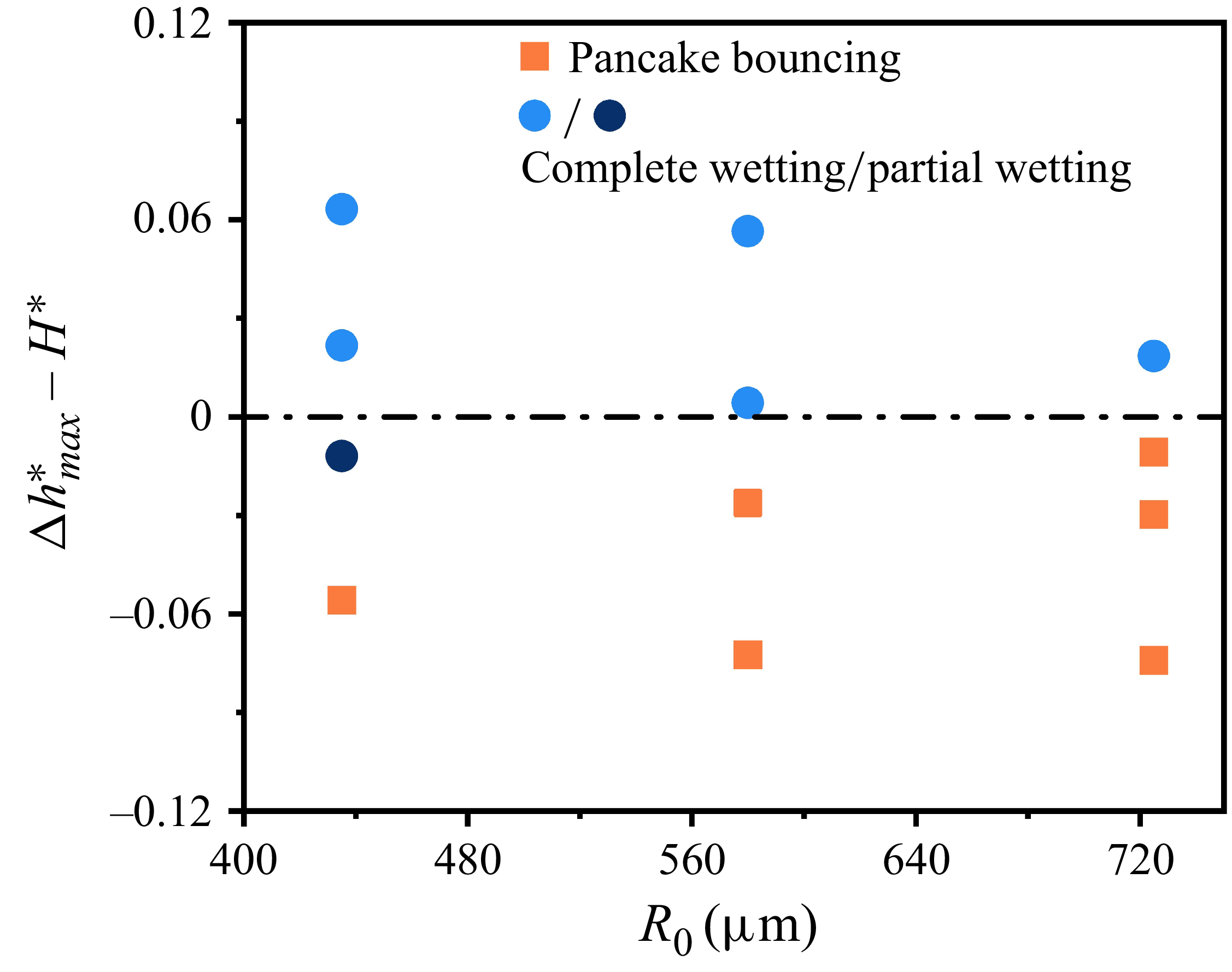
 R0
R0
 f=0.6 and H∗=0.17
 θeff
θeff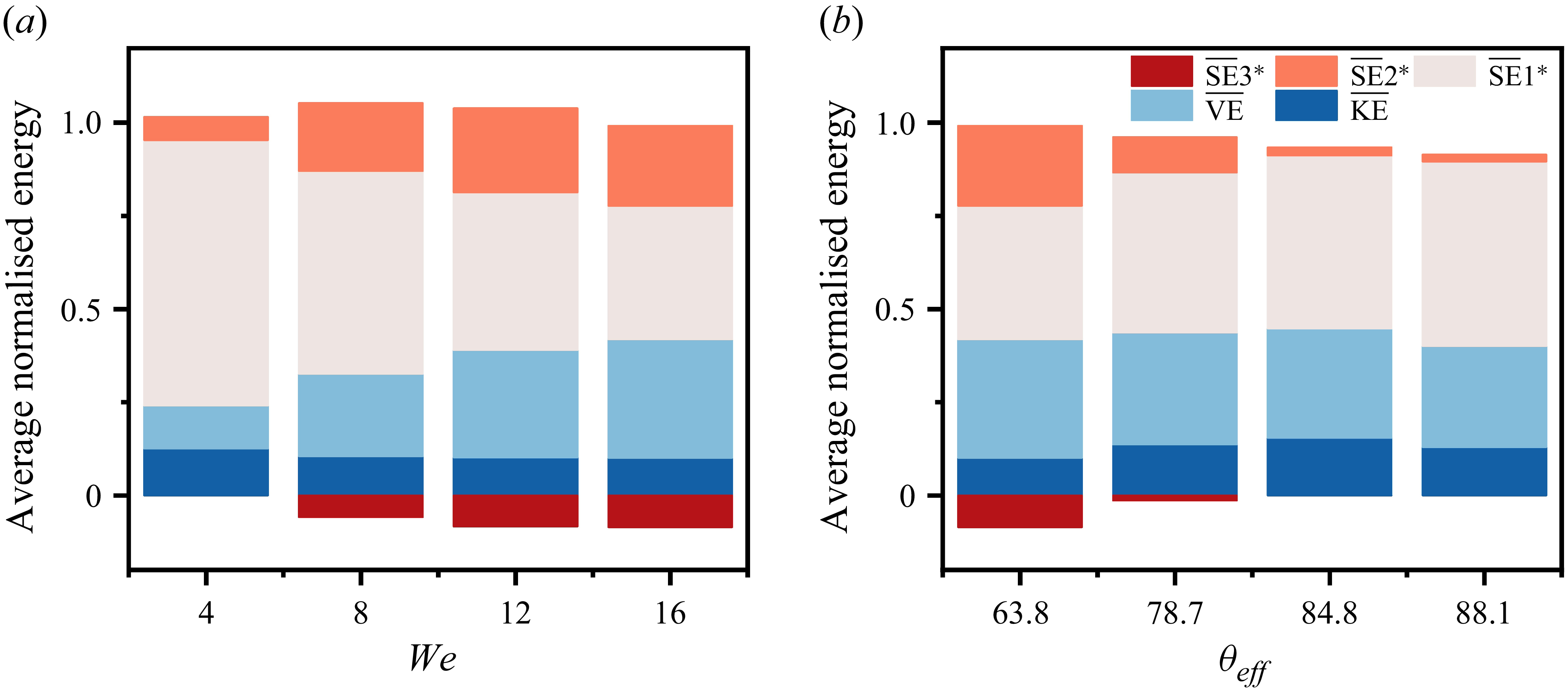
 θeff
θeff
 θ0
θ0 Heq∗)
Heq∗)

 Open access

