2 Flow simulation model

The lattice-Boltzmann method (LBM) solves the discrete form of the Boltzmann equation by using particle distribution functions to simulate the macroscopic flow properties. Through local integration of these particle distribution functions, the flow density, momentum and internal energy are obtained (Succi Reference Succi2001). The solution of the Boltzmann equation is performed on a Cartesian mesh (lattice), with an explicit time integration and collision model:

(2.1)$$\begin{eqnarray}f_{i}(\boldsymbol{x}+\boldsymbol{c}_{i}\unicode[STIX]{x0394}t,t+\unicode[STIX]{x0394}t)-f_{i}(\boldsymbol{x},t)=C_{i}(\boldsymbol{x},t),\end{eqnarray}$$

with $f_{i}$ representing the particle distribution function along the $i$th lattice direction. The particle motion is statistically described at a position $\boldsymbol{x}$ with a discrete velocity $\boldsymbol{c}_{i}$ in the $i$-direction at the time $t$. The space and time increments are represented by $\boldsymbol{c}_{i}\unicode[STIX]{x0394}t$ and $\unicode[STIX]{x0394}t$, respectively. For the collision term $C_{i}(x,t)$, the employed formulation is based on a Galilean invariant for thermal flows of non-unitary Prandtl number (Chen, Gopalakrishnan & Zhang Reference Chen, Gopalakrishnan and Zhang2014). The equilibrium Maxwell–Boltzmann distribution $f_{i}^{eq}$ is adopted (Chen, Chen & Matthaeus Reference Chen, Chen and Matthaeus1992). The distribution functions are projected on a basis of Hermite polynomials and the moments are computed over a discrete set of particle velocities, using Gaussian quadrature formulae for different lattices (Chen et al. Reference Chen, Gopalakrishnan and Zhang2014). For this work, a 19-state lattice, known as D3Q19, is adopted.

Given the high Reynolds number of the jet flow, a very-large-eddy simulation (VLES) model accounts for the unresolved scales of turbulence. A modified two-equation $k{-}\unicode[STIX]{x1D716}$ renormalization group (RNG) turbulence model is employed to compute a turbulent relaxation time that is added to the viscous relaxation time (Yakhot & Orszag Reference Yakhot and Orszag1986):

(2.2)$$\begin{eqnarray}\unicode[STIX]{x1D70F}_{eff}=\unicode[STIX]{x1D70F}+C_{\unicode[STIX]{x1D707}}\frac{k^{2}/\unicode[STIX]{x1D716}}{(1+\unicode[STIX]{x1D702}^{2})^{1/2}},\end{eqnarray}$$

where $C_{\unicode[STIX]{x1D707}}=0.09$, and $\unicode[STIX]{x1D702}$ is a combination of the local strain, local vorticity and local helicity parameters (Yakhot et al. Reference Yakhot, Orszag, Thangam, Gatski and Speziale1992). The term $\unicode[STIX]{x1D702}$ allows for the mitigation of the subgrid-scale viscosity, so that the resolved large-scale structures are not numerically damped. The relaxation time is then used to adapt the Boltzmann model to the characteristic time scales of a turbulent flow motion. Hence, the Reynolds stresses are not explicitly added to the governing equations, but they are an implicit consequence of the chaotic exchange of momentum driven by the turbulent flow, with characteristic times smaller than the slowly varying turbulent flow. The Reynolds stresses then have a nonlinear structure and are better suited to represent turbulence in a state far from equilibrium, as in the presence of distortion, shear and rotation (Chen et al. Reference Chen, Orszag, Staroselsky and Succi2004). A wall model is also adopted to approximate the no-slip boundary conditions, which is based on an extension of the generalized law-of-the-wall model, taking into account the effect of pressure gradients (Launder & Spalding Reference Launder and Spalding1974).

The low dissipation and dispersion of the LBM, coupled with a compressible and time-dependent solution, allow the sound field to be extracted directly from the pressure field (Brès, Pérot & Freed Reference Brès, Pérot and Freed2009). However, this approach would require a fairly large computational domain with respect to the nozzle and plate dimensions. A high degree of mesh refinement would also be necessary, even at regions far from the jet/surface, so that the number of points per wavelength would be sufficient for high-frequency far-field analyses. Therefore, to avoid high computational costs, the far-field noise is computed through the Ffowcs-Williams and Hawkings analogy (Ffowcs-Williams & Hawkings Reference Ffowcs-Williams and Hawkings1969), adopting the formulation 1A from Farassat & Succi (Reference Farassat and Succi1980), extended to a convective wave equation (Brès, Pérot & Freed Reference Brès, Pérot and Freed2010). The formulation is implemented in the time domain using a source-time-dominant algorithm (Casalino Reference Casalino2003).

A permeable surface is defined to include all the relevant noise sources, i.e. dipoles on the plate trailing edge and quadrupoles in the jet (da Silva et al. Reference da Silva, Deschamps, da Silva and Simões2015). Pressure and velocity fluctuations recorded on this surface are used for far-field noise estimation. A more detailed description of the FWH surface is reported in § 3.2. In addition, the FWH analogy can be applied to the pressure fluctuations on the solid plate surface, in order to isolate the noise contribution from the acoustic dipoles.

The methodology described above is implemented in the commercial software Simulia PowerFLOW 6-2019. This software has also been used and validated for aero-engine aeroacoustic applications to predict fan broadband noise in subsonic (Casalino, Hazir & Mann Reference Casalino, Hazir and Mann2017; Casalino et al. Reference Casalino, Avallone, Gonzalez-Martino and Ragni2019) and transonic (Gonzalez-Martino & Casalino Reference Gonzalez-Martino and Casalino2018) conditions. A validation study for the isolated SMC000 jet has been accomplished by van der Velden et al. (Reference van der Velden, Casalino, Gopalakrishnan, Jammalamadaka, Li, Zhang and Chen2018), showing a very good agreement with experimental results. For an installed jet, computations were performed by da Silva et al. (Reference da Silva, Deschamps, da Silva and Simões2015). The results, in terms of far-field noise spectra, also showed a good agreement with experimental data, indicating the capability of the solver to accurately predict JIN.

3 Numerical set-up

3.1 Installed jet configurations and flow conditions

The installed jet model replicates the NASA Glenn benchmark experiments (Brown Reference Brown2012; Podboy Reference Podboy2013), where a flat plate is placed in the vicinity of a single-stream jet nozzle (SMC000). The SMC000 is a round, convergent nozzle with an exit diameter $D_{j}=50.8~\text{mm}$, used for studies on subsonic jets (Brown & Bridges Reference Brown and Bridges2006). The primary convergent nozzle has a 152 mm diameter inlet, followed by a contraction with a $5^{\circ }$ taper angle up to the exit plane.

Figure 1.

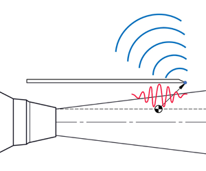
Schematic of the computational set-up, with the flat-plate length $L$ and height $h$. A permeable FWH surface encompasses the jet and the flat plate. Caps are placed at the downstream end of the surface, and cutouts are placed in the regions of the plate and nozzle.

Different geometric configurations are investigated, for which the length and height of the plate are varied. As shown in figure 1, the length $L$ is defined as the distance between the plate trailing edge and the nozzle exit plane, and the height $h$ as the radial position with respect to the jet centreline. The simulated cases are listed in table 1, marked with an X. For a given flat-plate length, the minimum radial position is determined based on a jet spreading angle of $7^{\circ }$ (Brown & Bridges Reference Brown and Bridges2006) to avoid grazing flow on the surface. The plate is 12.7 mm thick and it has a chamfer angle of $40^{\circ }$ at the trailing edge. It extends $0.75D_{j}$ upstream of the nozzle exit plane to avoid scattering effects at the leading edge. In the spanwise direction, the plate has a width of $36D_{j}$ to avoid side-edge scattering.

Table 1.

Investigated geometric cases, based on the flat-plate length $L$ and height $h$.

The simulated flow conditions are based on setpoints 01, 03 and 06 from the NASA wind tunnel experiments (Brown & Bridges Reference Brown and Bridges2006). All setpoints are characterized by subsonic jets with different acoustic Mach numbers ($M_{a}=U_{j}/c_{\infty }$). The jet flow characteristics are included in table 2, such as the nozzle pressure ratio (NPR), the temperature ratio $T_{R}$ (ratio between the jet and ambient static temperatures) and the Reynolds number $Re$, based on the nozzle exit diameter. Static flow parameters, such as ambient pressure and temperature, are taken from the work of Brown & Bridges (Reference Brown and Bridges2006).

Table 2.

Jet flow conditions for setpoints 01, 03 and 06 based on nozzle pressure ratio (NPR), acoustic Mach number $M_{a}$ and Reynolds number $Re$.

3.2 Computational set-up

The jet and the flat plate are placed in an almost quiescent domain, i.e. with a speed equal to 1 % of the jet exit velocity, at ambient pressure. This free-stream condition is added to avoid the situation in which eddies escaping the jet shear layer are trapped in the domain and do not dissipate, allowing the solver to operate and converge faster. This free-stream speed is considered negligible, compared to the jet velocity, and thus it does not alter the flow-field characteristics of the shear layer and the far-field noise. To generate the jet flow, an additional inlet boundary condition is placed $8D_{j}$ upstream of the nozzle exit plane (figure 1). The physical parameters used as boundary conditions are taken from experimental data (table 2). A zigzag trip, with a thickness of 1 mm ($0.02D_{j}$) and spacing of 1.62 mm ($0.03D_{j}$), is added inside the nozzle, $1.5D_{j}$ upstream of the exit plane, to force a fully turbulent boundary layer. This nozzle set-up was validated for the isolated jet case by van der Velden et al. (Reference van der Velden, Casalino, Gopalakrishnan, Jammalamadaka, Li, Zhang and Chen2018). The same strategy is adopted in this work for the installed case.

The main components of the set-up are shown in figure 1. A permeable FWH surface, represented by dashed lines, is used for the far-field noise computations. Its shape and dimensions are chosen such that the same surface can be used for all studied configurations. A length of $22D_{j}$ downstream of the nozzle exit plane and a width of $10D_{j}$ are used for the permeable surface to include all the sources of noise relevant for the current investigation.

Spurious effects due to hydrodynamic pressure fluctuations occurring on the FWH are avoided by placing cutouts at the nozzle and flat-plate regions. Additional sources caused by the jet crossing the downstream end of the FWH are mitigated by placing seven outflow surfaces (or end caps) at that region (figure 1). The far-field pressure signals obtained from each cap (located at different streamwise positions) are averaged, so that the spurious noise produced by the eddies crossing the permeable surface can be removed from the final far-field spectra (Brès et al. Reference Brès, Nichols, Lele and Ham2012).

Acoustic sponges, which consist of regions of increased viscosity, are added to the set-up in order to prevent wave reflection at solid boundaries and at the walls of the computational domain (Colonius, Lele & Moin Reference Colonius, Lele and Moin1997). Inside the nozzle, the sponge extends from the inlet plane up to $3.8D_{j}$ upstream of the exit plane. A spherical sponge with a diameter $130D_{j}$, centred at the nozzle exit plane and encompassing the entire geometry, is also added. A progressive coarsening of the grid towards the boundaries also contributes to the dampening of reflected acoustic waves.

The physical time of the simulations is divided into an initial transient, consisting of 10 flow passes through the FWH surface, and an acquisition time of 13 flow passes (total simulation time of 23 flow passes). The latter is defined based on the minimum output frequency to be analysed (defined as $St=0.04$), and the number of spectral averages (defined as 20), for an overlap coefficient of 0.5 in the fast Fourier transform (FFT) computation. For the finest grid resolution investigated, the physical time step is $1.5\times 10^{-7}~\text{s}$ for all setpoints, and the unsteady pressure on the FWH surface is sampled with a frequency of 416 kHz. The resultant physical simulation time and acquisition parameters are shown in table 3. The frequency resolution refers to the frequency band obtained from the FFT of the computed acoustic signals, based on the acquisition time and the selected number of averages.

Figure 2.

Far-field microphone positions: (a) 48 microphones in the polar array, divided for the reflected and shielded sides; (b) 12 microphones in the azimuthal array, normal to the jet axis. Microphone distances not to scale.

Table 3.

Simulation physical time and acquisition parameters for each setpoint.

Similarly as performed in the NASA benchmark experiments (Brown Reference Brown2012), the far-field noise levels are computed with a microphone arc array. The array is centred at the nozzle exit plane, with a radius of $100D_{j}$. Microphones are placed at an interval of $5^{\circ }$, ranging from $\unicode[STIX]{x1D703}=50^{\circ }$ to $\unicode[STIX]{x1D703}=165^{\circ }$ ($\unicode[STIX]{x1D703}=180^{\circ }$ corresponds to the jet axis). The noise levels are evaluated at both shielded and reflected sides of the plate, as shown in figure 2(a). An additional azimuthal array is located around the nozzle exit plane, normal to the jet axis, with 12 microphones spaced of $30^{\circ }$, as shown in figure 2(b).

4 Grid convergence and validation

A mesh convergence study is performed to assess the sensitivity of the numerical results to the discretization of the computational domain. The mesh resolution is defined as the number of voxels at the nozzle exit diameter. The resultant element size is used throughout the jet plume. Three grids are investigated: coarse ($\text{resolution}=32~\text{voxels}/D_{j}$), medium ($\text{resolution}=45~\text{voxels}/D_{j}$) and fine ($\text{resolution}=64~\text{voxels}/D_{j}$). The features of each grid are summarized in table 4. Details of the mesh set-up are reported in van der Velden et al. (Reference van der Velden, Casalino, Gopalakrishnan, Jammalamadaka, Li, Zhang and Chen2018).

Table 4.

Grid characteristics for convergence analysis.

The isolated and installed ($L=4D_{j}$ and $h=1D_{j}$) configurations, in the conditions of setpoint 03 ($M_{a}=0.5$), are used for the flow-field convergence study. The chosen installed case represents the configuration for which the surface is closest to the plume. Results are also compared with experimental data from Bridges & Wernet (Reference Bridges and Wernet2010) for validation. Flow-field measurements from particle image velocimetry are available for the isolated jet case (Bridges & Wernet Reference Bridges and Wernet2010). The absence of hydrodynamic interaction between the jet flow and the solid surface allows the use of these results for validation of all configurations. As can be appreciated from both the instantaneous flow realizations for the isolated and installed jet cases in figure 3, and the time-averaged velocity profiles and root mean square (r.m.s.) of velocity fluctuations in figure 4, no significant difference between isolated and installed configurations is found in either the jet-flow field or the centreline velocity profiles.

Figure 3.

Snapshots of the instantaneous flow field for (a) isolated and (b) installed jet configurations ($L=4D_{j}$ and $h=1D_{j}$). No visible change to the jet development is caused by the plate.

Figure 4.

Profiles of (a) time-averaged and (b) r.m.s. of fluctuations of the axial velocity component at the nozzle centreline for different grid resolutions, and compared to experimental data for setpoint 03.

From figure 4, it is shown that the potential core is well captured, compared to the experimental results, extending up to $6.5D_{j}$ from the exit plane. A small over-prediction of the velocity decay at the centreline, of the order of $0.04U_{j}$, is also found. Minor deviations in velocity amplitude are also seen between the medium and fine isolated cases around $12<x/D_{j}<15$, probably due to the strong unsteadiness of the flow in that region. Similarly, both the amplitude and the spatial development of the turbulent velocity fluctuations are well captured, with minor differences between the three grids and the experimental results. It is conjectured that these small deviations in the velocity r.m.s. occur due to the turbulence properties set at the nozzle inlet, which do not match perfectly the experimental conditions.

A key element for assessing the quality of the simulation is that turbulence in the mixing layer is accurately resolved in the frequency range of interest. The spectrum of turbulent kinetic energy $E$ versus Strouhal number ($St=f\times D_{j}/U_{j}$), obtained for setpoint 03, is shown in figure 5 for two probes placed at the nozzle lipline ($y=0.5D_{j}$) of the isolated jet, at positions $x=5D_{j}$ and $x=10D_{j}$. The spectra are shown to follow Kolmogorov’s $5/3$ decay law up to high frequencies, of the order of $St=2$ (6.7 kHz). These results indicate that the turbulence characteristics are correctly modelled and the resultant spectral analyses, including the far-field noise resultant from turbulent mixing, are reliable.

Figure 5.

Spectra of turbulent kinetic energy for two probes at the nozzle lipline ($y=0.5D_{j}$) of the isolated jet (setpoint 03).

The far-field spectra for the installed configuration are compared to the experimental results from Brown (Reference Brown2012). For the comparisons, an intermediate case ($L=4D_{j}$ and $h=1.25D_{j}$ at setpoint 03) is chosen. The narrowband sound pressure level (SPL), obtained for a constant frequency band of 100 Hz, is plotted against the Strouhal number in figure 6. Results are displayed for the reflected side of the plate (refer to figure 2a), at two polar angles: $\unicode[STIX]{x1D703}=90^{\circ }$, i.e. the sideline direction, and $\unicode[STIX]{x1D703}=150^{\circ }$, i.e. near the direction of the jet axis. A reference pressure of $2\times 10^{-5}~\text{Pa}$ is used for the conversion to decibels (dB). The frequency band of the experimental data has also been changed from 12.2 Hz to 100 Hz, so that it is comparable with the simulation results.

The spectral shape is correctly predicted by the simulations from all grids, at both polar angles. At low and mid-frequencies, the curves for the medium and fine grids display similar amplitudes, and convergence is achieved. For high frequencies, the effect of grid resolution is more evident, and it is related to the cutoff frequency. For the coarse mesh, the cutoff frequency occurs at $St\approx 1.8$, whereas, for the fine case, it occurs at $St\approx 3$, based on the chosen element sizes. At frequencies higher than $St=3$, there is less agreement between the numerical (fine case) and experimental results, probably due to grid resolution effects. Up to this frequency, which is the range of interest, the maximum deviation between the results of the fine mesh and the experiments is approximately 4 dB. This shows the capability of the model to correctly predict JIN with sufficient accuracy. The results shown in the next sections of this paper are therefore obtained from the fine resolution grid so that analyses can be performed up to high frequencies ($St<3$).

5 Installation effects and trailing-edge scattering

The far-field SPL for the isolated and installed jets ($L=4D_{j}$ and $h=1D_{j}$) at setpoint 03 are plotted versus the Strouhal number in figure 7. The spectra are obtained for a constant frequency band of 100 Hz, and at polar angles $\unicode[STIX]{x1D703}=\pm 90^{\circ }$ and $\unicode[STIX]{x1D703}=\pm 150^{\circ }$.

Figure 6.

Grid convergence and validation of aeroacoustic results for the installed jet ($L=4D_{j}$ and $h=1.25D_{j}$). Spectra obtained for the reflected side of the plate at (a) $\unicode[STIX]{x1D703}=90^{\circ }$ and (b) $\unicode[STIX]{x1D703}=150^{\circ }$ and setpoint 03.

Figure 7.

Far-field spectra of the installed jet ($L=4D_{j}$ and $h=1D_{j}$), at the reflected and shielded sides of the plate, at (a) $\unicode[STIX]{x1D703}=\pm 90^{\circ }$ and (b) $\unicode[STIX]{x1D703}=\pm 150^{\circ }$, compared to the isolated configuration (setpoint 03).

In the sideline direction ($\unicode[STIX]{x1D703}=\pm 90^{\circ }$), installation effects result in low-frequency noise amplification, up to $St=0.7$. The maximum increase, relative to the isolated case, is 14 dB at $St=0.19$. In the frequency range $0.05<St<0.7$, the spectra at the reflected and shielded sides display similar shape and amplitude, in agreement with Head & Fisher (Reference Head and Fisher1976). This confirms that, for this frequency range, the dominant noise generation mechanism is the scattering of the near-field hydrodynamic waves at the trailing edge of the flat plate. For $St>0.7$, the spectra for the installed cases are dominated by quadrupole noise sources. At the reflected side, noise levels are approximately 3 dB higher than those of the isolated case, as expected from the reflection on a half-plane (Cavalieri et al. Reference Cavalieri, Jordan, Wolf and Gervais2014). For $\unicode[STIX]{x1D703}=\pm 150^{\circ }$, i.e. towards the jet axis, installation effects are no longer visible and the spectra are similar to that of the isolated jet.

To determine the dominant noise sources for each configuration, instantaneous dilatation field contours for the jet at setpoint 03 are shown in figure 8(a,b). They are obtained for a frequency band of $0.18<St<0.21$, corresponding to the region of maximum noise increase due to installation effects. Contours are saturated so that pressure waves outside of the jet plume can be identified.

Figure 8.

Contours of the time derivative of the pressure field of isolated and installed jets, bandpass-filtered over a frequency range $0.18<St<0.21$. Contours are saturated so that pressure waves outside of the jet plume can be identified.

For the isolated case, the dilatation field shows pressure waves convecting with the jet. Given the low Mach number investigated ($M_{a}=0.5$), it is expected that a large portion of those waves convect at subsonic speeds. A distinct change of their amplitude, characterized by growth, saturation (peak region) and decay, can be observed. Therefore, due to this spatial modulation, a small portion of the energy of the waves in the evanescent near pressure field propagates to the far field as noise (Jordan & Colonius Reference Jordan and Colonius2013). For the installed jet, additional acoustic waves are generated due to scattering at the plate trailing edge. Waves on the shielded and reflected sides of the plate have opposite sign, indicating a phase shift of $\unicode[STIX]{x03C0}$, as described by Head & Fisher (Reference Head and Fisher1976) and Cavalieri et al. (Reference Cavalieri, Jordan, Wolf and Gervais2014). These scattered waves then propagate in the upstream direction of the jet.

The previous observations are confirmed by the directivity plots of overall sound pressure level (OASPL), integrated in the range $0.05<St<3$, shown in figure 9. In the polar direction (figure 9a), the maximum noise increase occurs at $\unicode[STIX]{x1D703}\approx \pm 50^{\circ }$. Smaller angles could not be computed due to the presence of the nozzle, which acts as a shielding body. However, the trend is consistent with the cardioid directivity, proposed by Ffowcs-Williams & Hall (Reference Ffowcs-Williams and Hall1970). Approaching the jet axis, the curves for the isolated and installed cases collapse, confirming that the quadrupole sources dominate. In the azimuthal direction, the OASPL values are plotted normal to the jet axis, for a fixed polar angle of $\unicode[STIX]{x1D703}=90^{\circ }$. The isolated jet displays an axisymmetric behaviour, with similar noise levels at all azimuthal angles. For the installed jet, a maximum noise increase of 5 dB is obtained in the direction normal to the flat plate ($\unicode[STIX]{x1D719}=\pm 90^{\circ }$), whereas no difference is present for $\unicode[STIX]{x1D719}=0^{\circ }$ and $\unicode[STIX]{x1D719}=180^{\circ }$. For intermediate angles, a small difference is visible between the upper and lower sides, due to shielding and reflection effects. This directivity pattern is consistent with the presence of acoustic dipoles, with axes perpendicular to the surface, in agreement with Head & Fisher (Reference Head and Fisher1976).

Figure 9.

(a) Polar and (b) azimuthal directivities of the isolated and installed jets ($L=4D_{j}$ and $h=1D_{j}$) for setpoint 03.

Spectra of surface pressure fluctuations for probes placed at the trailing edge and leading edge of the plate are plotted in order to verify that trailing-edge noise is the dominant source. The spectra in terms of pressure power amplitude (pressure squared), non-dimensionalized by the square of the jet nominal dynamic pressure ($q=0.5\unicode[STIX]{x1D70C}U_{j}^{2}$), are shown in figure 10. There is a large difference in amplitude between the curves, of approximately three orders of magnitude. This indicates that there are no significant hydrodynamic fluctuations at the leading edge, and, consequently, scattering at the leading edge has minor effects on the overall acoustic field.

Figure 10.

Far-field spectra of pressure fluctuations on probes at the leading and trailing edges of the plate, at the jet symmetry plane, obtained for setpoint 03.

Figure 11.

Far-field spectra of the installed jet ($L=4D_{j}$ and $h=1D_{j}$), at the reflected and shielded sides of the plate, compared to the isolated configuration for (a) setpoint 01 ($M_{a}=0.35$) and (b) setpoint 06 ($M_{a}=0.80$), for polar angles $\unicode[STIX]{x1D703}=\pm 90^{\circ }$.

The sound pressure levels of the installed jet ($L=4D_{j}$ and $h=1D_{j}$) for the other setpoints are plotted with the respective isolated configuration spectra in figure 11, for polar angles $\unicode[STIX]{x1D703}=\pm 90^{\circ }$. For the low-Mach-number jet ($M_{a}=0.35$), shown in figure 11(a), a strong amplification occurs at low frequencies, similar to the previous results for setpoint 03. At the spectral peak ($St=0.26$), there is a difference of 19 dB between installed and isolated noise levels. The spectra for shielded and reflected sides show similar values up to $St=0.77$, which marks the maximum frequency for which the scattering at the trailing edge is the dominant source. For the high-Mach-number case ($M_{a}=0.8$), installation effects result in a lower amplification with respect to the isolated case at the spectral peak (5 dB at $St=0.4$). This is due to the dependence of the sound intensity with the jet velocity, which is $U_{j}^{5}$ for the scattering (Ffowcs-Williams & Hall Reference Ffowcs-Williams and Hall1970) and $U_{j}^{8}$ for turbulence-mixing noise (Lighthill Reference Lighthill1952). Therefore, with a high-velocity jet, the spectrum is dominated by the isolated jet noise due to turbulent mixing.

The influence of the solid plate geometry on the installed far-field noise is also assessed. Results pertaining to the change of the plate radial position relative to the jet centreline are shown in figure 12, for the three investigated plate lengths and $M_{a}=0.5$. The spectra, plotted for $\unicode[STIX]{x1D703}=90^{\circ }$ (reflected side of the plate), show that moving the surface away from the plume results in lower noise levels, especially at mid-frequencies. For the case with $L=4D_{j}$, there is a decrease of 4 dB between $h=1D_{j}$ and $h=1.25D_{j}$, and 6 dB between $h=1D_{j}$ and $h=1.5D_{j}$ at the spectral peak ($St=0.2$). Similar trends occur for other plate lengths and jet setpoints. The cross-over point with respect to the isolated jet curve also moves to higher frequencies for surfaces closer to the jet. For $L=4D_{j}$, the cross-over shifts from $St=0.33$ ($h=1.5D_{j}$) to $St=0.70$ ($h=1D_{j}$). This is probably due to the increased proximity of the surface to smaller-scale eddies that generate higher-frequency noise when scattered.

Figure 12.

Effect of changing the plate radial position on the far-field noise levels. Spectra are plotted for different plate lengths of (a) $L=4D_{j}$, (b) $L=5D_{j}$ and (c) $L=6D_{j}$, at a polar angle $\unicode[STIX]{x1D703}=90^{\circ }$ (reflected side) and for $M_{a}=0.5$.

Figure 13.

Effect of changing the plate length on the far-field noise levels. Spectra are plotted for different plate heights of (a) $h=1.25D_{j}$ and (b) $h=1.5D_{j}$, at a polar angle$\unicode[STIX]{x1D703}=-90^{\circ }$ (shielded side) and for $M_{a}=0.5$.

The effect of changing the plate length is shown in figure 13. Spectra are obtained for three surface lengths, at fixed radial positions $h=1.25D_{j}$ and $h=1.5D_{j}$, for $\unicode[STIX]{x1D703}=-90^{\circ }$ and $M_{a}=0.5$. It is shown that, for longer surfaces, noise increase is higher at low frequencies, with a difference of 7 dB between the curves for $L=6D_{j}$ and $L=4D_{j}$, for $h=1.25D_{j}$ and $St=0.15$. For longer plates, the spectral peak also moves towards lower frequencies: for $h=1.25D_{j}$ the spectral peak is at $St=0.18$ and $0.15$ for the shortest and longest plates, respectively. This is due to the increase of energy content of large-scale structures in the mixing layer in the downstream direction of the jet (Lawrence et al. Reference Lawrence, Azarpeyvand and Self2011). Since these structures generate low-frequency hydrodynamic pressure waves, the scattering effects are also amplified in that frequency range. At frequencies higher than $St=0.2$, the difference between the curves is small, and the cross-over frequency with the isolated curve is not significantly changed for different plate lengths. At high frequencies, the scattering is not strongly affected by changing the surface length since small-scale structures show similar characteristics and amplitude in the streamwise direction (Arndt et al. Reference Arndt, Long and Glauser1997).

The results show that the far-field noise of the installed case is dependent on the characteristics of the near field of the jet and the position of the trailing edge. The phenomena behind JIN are therefore investigated in the next sections, linking the edge scattering phenomenon with jet near-field properties at the trailing-edge region.

6 Effect of source characteristics on jet-installation noise

The goal of this section is to identify the frequency range in which JIN is the dominant noise source, for a given plate length and radial position, starting from near-field data of the isolated jet.

This is performed by making use of the inequalities proposed by Ffowcs-Williams & Hall (Reference Ffowcs-Williams and Hall1970). They found that, for a half-plane, noise amplification is caused by the scattering of eddies within a wavelength from the edge; this satisfies the inequality $2kr_{0}\ll 1$, where $k$ is the wavenumber and $r_{0}$ is the distance from the centre of the eddy to the edge of the half-plane. On the other hand, for eddies far from the edge, which satisfy the inequality $(kr_{0})^{1/2}\gg 1$, there is no noise increase due to scattering. These parameters can then be regarded as a measure of source compactness, based on the Helmholtz number $kr_{0}$, which is dependent on the distance between the source and the edge. As a consequence, once this distance is known, a wavenumber envelope of flow structures that are effectively scattered at the trailing edge can be found.

To compute the envelope, an equivalent hydrodynamic source distant $r_{0}$ from the plate trailing edge is used, for a given wavenumber, as shown in figure 14. It is assumed that this equivalent source is located within the jet mixing layer, positioned at $(x_{source},y_{source})$. The radial position of the source is assumed to be at the nozzle lipline ($y_{source}\approx 0.5D_{j}$), which corresponds to the centre of the mixing region in the jet shear layer, i.e. the region of maximum amplitude of hydrodynamic fluctuations (Arndt et al. Reference Arndt, Long and Glauser1997). In more detail, the hypothesis assumes that small changes in the radial position of the equivalent source (around the lipline) are negligible with respect to the distance from the edge. The remaining variable, $x_{source}$, is determined by using the near-field pressure spectra of the isolated jet (Arndt et al. Reference Arndt, Long and Glauser1997).

Figure 14.

Sketch representation of an equivalent source located in the centre of the jet mixing layer (assumed to be the nozzle lipline), at a certain distance $r_{0}$ from a defined measurement point (plate trailing edge), for a given wavenumber.

Figure 15.

Near-field pressure spectrum at $x=4D_{j}$ and $y=1.5D_{j}$. At low frequencies, the spectrum display amplitudes increasing with frequency up to the spectral peak (energy-containing region), followed by a decay (inertial subrange). At higher frequencies, the pressure fluctuations display acoustic behaviour.

Following Arndt et al. (Reference Arndt, Long and Glauser1997), the pressure spectrum in the near field of an isolated jet can be divided into three regions (figure 15). At low frequencies, there is an energy-containing region, characterized by amplitude slowly increasing with frequency. This region extends up to the spectral peak, and then it is followed by the inertial subrange, where there is a steep amplitude decay. Finally, there is the acoustic region, where pressure fluctuations of this type are dominant. The intensity of the pressure fluctuations scales as

(6.1)$$\begin{eqnarray}I\propto \unicode[STIX]{x1D70C}_{0}a_{0}U_{0}^{2}(kr_{0})^{n},\end{eqnarray}$$

where $\unicode[STIX]{x1D70C}_{0}$ is the fluid density, $a_{0}$ is the speed of sound and $U_{0}$ is the source velocity. For the energy-containing region, where the sources display hydrodynamic behaviour, $n=-6$. For the inertial subrange, $n=-6.67$ to take into account the spectral decay with frequency. Finally, when $n=-2$, the sources display an acoustic behaviour (Arndt et al. Reference Arndt, Long and Glauser1997).

Since JIN is correlated to hydrodynamic pressure fluctuations (Papamoschou Reference Papamoschou2010), $x_{source}$ can be found by fitting the amplitude of pressure fluctuations from a set of near-field spectra of the isolated jet, for a given wavenumber. For a given plate length with the trailing edge located at $x_{m}$, the procedure for the fitting is the following:

1. (i) spectra in the near field of the isolated jet dataset are extracted at different radial positions ($y_{m}$);

2. (ii) a source position ($x_{source}$) is assumed upstream of $x_{m}$;

3. (iii) the Helmholtz number ($kr_{0}$) is computed at the radial locations defined in (i), using the source position from (ii);

4. (iv) for a given $St$ chosen as input, the exponent of $\hat{P}\propto (kr_{0})^{n}$, i.e. along the $r_{0}$ direction, as described in (6.1), is computed; and

5. (v) if $n\neq -6$, $x_{source}$ is shifted and the exponent is recomputed; when $n=-6$, the source position is converged.

An example of the method is shown in figure 16(a), where a set of near-field spectra extracted at $x_{m}=4D_{j}$ and at different radial stations, for setpoint 03 ($M_{a}=0.5$), is reported. After a source position is converged for a chosen frequency value, spectra are represented as a function of $kr_{0}$, as shown in figure 16(b). The thin black dotted line represents the slope of $kr_{0}^{-6}$, crossing the points of constant frequency $St=0.2$ for each radial position $y$. For this specific frequency and measurement point, the axial position of the source is found at $x_{source}=0.9x_{m}$, or $x_{source}=3.6D_{j}$. This analysis is then carried out similarly at other frequencies, and for the two other axial measurement positions ($x_{m}=5D_{j}$ and $x_{m}=6D_{j}$), as shown in figure 17. Similar trends are obtained for the other setpoints ($M_{a}=0.35$ and $M_{a}=0.8$).

It is shown that, for increasing frequency, the equivalent source position moves towards $x_{m}$ for all analysed cases. These results show that small-scale equivalent sources need to be positioned axially closer to the trailing-edge location in order to generate hydrodynamic pressure fluctuations able to scatter as noise at that point.

Figure 16.

Near-field pressure spectra at different radial positions for the calculation of source-edge distance, obtained at $x=4D_{j}$ and $M_{a}=0.5$. (a) Spectra as a function of Strouhal number. (b) Spectra as a function of the Helmholtz number $kr_{0}$, based on a converged equivalent source position. The thin dotted line represents a $r_{0}^{-6}$ (hydrodynamic characteristic) slope on the pressure data for a constant frequency $St=0.2$.

Figure 17.

Equivalent source position, obtained for different frequencies and axial measurement positions $x_{m}$, for setpoint 03. For increasing frequency, the equivalent source moves towards $x_{m}$.

The determination of the equivalent source position allows for the computation of an equivalent distance between source and measurement points, which can be used in the compactness analogy defined by Ffowcs-Williams & Hall (Reference Ffowcs-Williams and Hall1970). The plots in figures 18(a) and 18(b) show the dependence with frequency of the parameters $2kr_{0}$ (eddies near the edge) and $kr_{0}^{1/2}$ (eddies far from the edge), respectively. Results are included for the three jet setpoints and four geometrical cases. A dotted line is also included to mark the points where the curves are equal to 1. It can be seen that the values of both parameters increase with frequency, for all conditions. For $M_{a}=0.5$ and a case with $L=4D_{j}$ and $h=1D_{j}$, the condition $2kr_{0}$ reaches 1 for a frequency $St=0.21$. For the other cases, this occurs at lower frequencies ($St\approx 0.17$). For the same case, the other condition $kr_{0}^{1/2}$ reaches 1 for a frequency $St=0.65$ with a similar trend for the other cases. Therefore, it is concluded that there is a frequency range in each case where neither condition defined by Ffowcs-Williams & Hall (Reference Ffowcs-Williams and Hall1970) is satisfied. In this transition region, a less efficient scattering at the edge (lower sound amplification) is expected due to the structures becoming increasingly compact.

Figure 18.

Compactness parameters ($2kr_{0}$ and $kr_{0}^{1/2}$) as a function of frequency, obtained for different measurement points at three jet acoustic Mach numbers. A dotted line is included to determine the frequency where these parameters are equal to 1.

For a better understanding of the physical meaning of these two compactness conditions and how they relate to the produced noise, isolated and installed far-field spectra are plotted in figure 19, highlighting the frequencies where the compactness parameters are equal to 1 with dotted lines. The spectra are obtained for $M_{a}=0.5$ at the shielded side of the plate $(\unicode[STIX]{x1D703}=-90^{\circ })$, for a better visualization of the cross-over frequency between the installed and isolated curves.

Figure 19.

Far-field spectra with the frequency values where the compactness parameters $2kr_{0}$ and $kr_{0}^{1/2}$ are equal to 1, for different plate geometries, as indicated below each panel. The former approaches the peak frequency, whereas the latter approaches the cross-over between installed and isolated curves. Spectra obtained for $\unicode[STIX]{x1D703}=-90^{\circ }$ and $M_{a}=0.5$.

The compactness parameters relate to the far-field spectra in two different manners. The frequency limit for eddies very near the edge ($2kr_{0}=1$) occurs approximately at the location of the peak noise levels for the installed configuration. This is valid for all investigated configurations, and it indicates that the maximum amplification occurs at the limit Helmholtz number where the structures are regarded as non-compact with respect to the edge distance. On the other hand, the frequency limit for eddies far from the edge ($(kr_{0})^{1/2}=1$) occurs approximately at the location where the far-field noise levels for the installed configuration cross the curve of the isolated jet. This is consistent with the analytical formulation of Ffowcs-Williams & Hall (Reference Ffowcs-Williams and Hall1970), which states that eddies far from the edge produce noise levels equivalent to that of free turbulence, when effects of shielding and reflection by the surface are disregarded. Finally, the transition region, where neither inequality is satisfied, is characterized by a decay in noise levels with increasing frequency.

Spectra for two geometric cases, obtained for the other jet setpoints and $\unicode[STIX]{x1D703}=-90^{\circ }$, are plotted in figure 20. Similar trends are obtained for other configurations. The results for $M_{a}=0.35$ are in agreement with those obtained previously for $M_{a}=0.5$, where the condition $2kr_{0}=1$ occurs at a frequency near the spectral peak, and $kr_{0}^{1/2}=1$ occurs near the cross-over between isolated and installed curves. For $M_{a}=0.8$, however, this approach does not provide the same conclusions. While the cross-over frequency is still predicted fairly accurately, the first condition does not predict the spectral peak ($St=0.4$, for $L=4D_{j},h=1D_{j}$), but rather a much lower frequency ($St=0.12$).

Figure 20.

Far-field spectra with the frequency values where the compactness parameters $2kr_{0}$ and $kr_{0}^{1/2}$ are equal to 1, for $M_{a}=0.35$ (a,b) and $M_{a}=0.80$ (c,d). Spectra obtained for $\unicode[STIX]{x1D703}=-90^{\circ }$.

To better understand the reasons behind the discrepancy, figure 21 reports spectra for the isolated and installed configurations, at $\unicode[STIX]{x1D703}=-90^{\circ }$, along with those obtained by integrating only the surface pressure fluctuations on the plate using the FWH solid formulation (Ffowcs-Williams & Hawkings Reference Ffowcs-Williams and Hawkings1969). The latter only accounts for dipole sources on the plate, and thus noise from quadrupoles in the jet is disregarded. The spectra are computed on the upper (shielded side) and lower (reflected side) surfaces, separately, as well as considering the entire plate. On the upper side of the plate, two peaks are visible at $St=0.12$ and $St=0.4$, with similar amplitudes. The former occurs approximately at the frequency predicted by the method proposed in this section. The second spectral peak, which is dominant on the lower side of the plate, suggests that other sources of sound in addition to trailing-edge scattering might be present.

Figure 21.

Far-field spectra of the isolated and installed jets, with the noise from pressure fluctuations computed on the overall surface, and on the upper and lower sides separately. Spectra obtained for $\unicode[STIX]{x1D703}=-90^{\circ }$ and $M_{a}=0.8$.

It is concluded that the main characteristics of the frequencies related to JIN are related to the degree of compactness of the sources with respect to their distance to the scattering point. As a reminder, the methodology of this section provides information on the peak frequency of installation effects, as well as the maximum frequency where the trailing edge is the dominant source. This information can be used for assessing installation effects, solely with data from the isolated jet.

7 Far-field noise scaling based on near-field properties

In this section, the effect of near-field properties on the spectral amplitude of an installed jet is addressed. This is performed by finding scaling laws for the far-field spectra for different geometric cases, using only information from the isolated jet. Those scaling laws are deemed to predict the far-field noise independently of the geometric configuration adopted for the plate, reducing the need for testing or computing several cases. First, a scaling law is found for moving the plate in the radial direction, and afterwards for changing the plate length.

7.1 Radial-direction scaling law

The far-field noise data in figure 12 show higher noise levels and a broader frequency range of amplification when the surface is closer to the jet in the radial direction. To relate this behaviour to the near-field characteristics of the isolated jet, spectra of pressure fluctuations from the latter are computed at several locations outside of the plume, similarly as shown in figure 16(a). To determine how the pressure fluctuations for an isolated jet vary in the radial direction, they are plotted against $y$ in figure 22 for $M_{a}=0.5$. The curves display the decay at the axial position of $x=4D_{j}$ and frequencies equal to $St=0.2$ and $St=0.4$ (selected in the noise amplification region for the installed configuration with $h=1D_{j}$).

Figure 22.

Near-field decay of pressure fluctuations in the radial direction for an isolated jet, at $St=0.2$ and $St=0.4$, at an axial position $x=4D_{j}$ and for $M_{a}=0.5$.

Strong fluctuations occur at $y=0.5D_{j}$, a location that corresponds to the nozzle lipline. This is in agreement with the assumption made in the previous section that the lipline can be considered the centre of the structures in the mixing layer. Moving away from the jet axis, the near pressure field in the radial direction can be divided into three regions: a nonlinear hydrodynamic field, a linear hydrodynamic field and an acoustic field (Arndt et al. Reference Arndt, Long and Glauser1997). The first one is characterized by the flow inside the plume and nearby regions. Further away from the jet, the hydrodynamic pressure fluctuations display an exponential decay in the $y$-direction. For $St=0.2$, the linear hydrodynamic region is placed in the range $1<y/D_{j}<2.7$, whereas for $St=0.4$ it occurs closer to the plume, in the range $0.8<y/D_{j}<2.2$. Finally, even farther from the jet, pressure fluctuations display acoustic wave characteristics and an algebraic decay (Arndt et al. Reference Arndt, Long and Glauser1997). These results are in agreement with measurements performed in the near field of a jet (Arndt et al. Reference Arndt, Long and Glauser1997; Suzuki & Colonius Reference Suzuki and Colonius2006; Tinney & Jordan Reference Tinney and Jordan2008). The position and extension of the linear hydrodynamic field, which is the most relevant for this work, are shown to be frequency-dependent. At higher frequencies, the linear decay is steeper and the far field begins closer to the jet. This is consistent with the results from the previous section, where it was shown that small-scale structures become quickly compact when moving away from the lipline. Similar trends are obtained for the other setpoints.

Figure 23.

Far-field spectra of installed jets, scaled by the exponential of the plate radial position ($L=4D_{j}$ and $\unicode[STIX]{x1D703}=90^{\circ }$), for $M_{a}=0.5$. (a) Only the amplitude of the curves is scaled. (b) The amplitude is scaled and the curves are offset to match the spectral peak.

In the linear hydrodynamic region, the pressure fluctuations show an exponential pressure decay. Therefore, the installed far-field noise levels can be scaled with $\text{e}^{h}$, based on the respective plate height for each case. This is shown in figure 23(a), where there is a fairly good agreement between the curves for $0.18<St<0.65$. For $St>0.65$, the curves diverge since this region of the spectra is dominated by noise from quadrupole sources reflected on the surface. In the previous sections, it was shown that the spectral peak changes for plates at different radial positions. Therefore, if the scaled spectra are offset in frequency, a better agreement between the curves is found, as shown in figure 23(b). In these plots, the scaled SPL spectra ($\text{SPL}\times \text{e}^{h}$) for $h=1.25D_{j}$ and $h=1.5D_{j}$ are offset in frequency (‘Offset $St$’) so that their peak matches that of $h=1D_{j}$.

It is then concluded that a combination of amplitude and frequency scaling is necessary to match the noise levels of different radial configurations. While the amplitude can be easily scaled with the exponential of the plate height, knowledge of the spectral peak frequency is necessary beforehand. The method described in the previous section can provide a fairly good prediction of the spectral peak for low/mid-Mach-number jets, and thus it can be used together with the amplitude scaling in order to obtain the far-field spectra of different geometric configurations. This scaling is also applied for plates with different lengths ($L=5D_{j}$ and $L=6D_{j}$) as shown in figure 24, with a good agreement between the curves. Scaled spectra for the other jet setpoints are shown in figure 25. For these other conditions there is also a good agreement between the curves. For $M_{a}=0.8$, however, there is a slight difference in amplitude, particularly at low frequencies ($St<0.1$), possibly due to effects from sources other than scattering.

Figure 24.

Far-field spectra of installed jets, scaled by the exponential of the plate radial position, for $\unicode[STIX]{x1D703}=90^{\circ }$ and $M_{a}=0.5$. (a) $L=5D_{j}$, (b) $L=6D_{j}$.

Figure 25.

Far-field spectra of installed jets ($L=4D_{j}$), scaled by the exponential of the plate radial position, for $\unicode[STIX]{x1D703}=90^{\circ }$. (a) $M_{a}=0.35$, (b) $M_{a}=0.8$.

7.2 Axial-direction scaling law

A similar procedure is carried out to find a scaling law for the noise generated by plates with different lengths. Spectra of near-field pressure fluctuations computed at different axial locations, for $y=1.5D_{j}$ and $M_{a}=0.5$, are shown in figure 26(a). The results show an increase of low-frequency fluctuations at positions farther from the nozzle exit plane due to the presence of highly energetic large-scale structures. It can be noticed that, aside from $x=3D_{j}$, the curves tend to collapse at $St\approx 0.45$, suggesting that, at high frequencies, the amplitude of the pressure fluctuations remains constant in the axial direction.

Figure 26.

(a) Near-field pressure spectra. (b) Progression of near-field pressure in the axial direction. Data obtained for $y=1.5D_{j}$ and $M_{a}=0.5$.

This behaviour can be better visualized by plotting the amplitude of the pressure fluctuations in the axial direction for specific frequencies (figure 26b). At relatively low frequencies ($St=0.20$ and $St=0.28$), the amplitude of pressure fluctuations increases in the axial direction. Owing to the large wavelength associated with these structures, they grow and saturate at positions farther from the nozzle exit plane when compared to small-scale eddies. A nonlinear behaviour is also found downstream of $x=8D_{j}$ due to the presence of the rotational flow inside of the jet plume. At higher frequencies, the amplitude of the pressure fluctuations saturates and remains constant in the axial direction. This plateau is due to the contamination of the signal by the jet acoustic waves (Suzuki & Colonius Reference Suzuki and Colonius2006). If only the coherent, hydrodynamic fluctuations were present, a decay would be expected to follow the saturation point due to the wavepacket nature of the jet (Crighton & Huerre Reference Crighton and Huerre1990). Therefore, after the saturation point, acoustic fluctuations, which have a slower decay rate, become dominant with respect to hydrodynamic ones.

To remove the contribution of non-coherent fluctuations in the near field, a frequency domain form of POD, known as SPOD, is applied (Schmidt et al. Reference Schmidt, Towne, Rigas, Colonius and Brès2018; Towne et al. Reference Towne, Schmidt and Colonius2018), similarly as done in other studies on jet noise (Arndt et al. Reference Arndt, Long and Glauser1997; Tinney & Jordan Reference Tinney and Jordan2008; Breakey et al. Reference Breakey, Jordan, Cavalieri, Léon, Zhang, Lehnasch, Colonius and Rodríguez2013). SPOD is preferred to space-only POD because it can properly describe spatiotemporal coherent structures, due to its spectral-based kernel. In this way, the flow is decomposed at different time scales and, consequently, the characteristics of the structures can be analysed for each frequency band (Towne et al. Reference Towne, Schmidt and Colonius2018), which is necessary for a posterior scaling of the far-field noise. Moreover, due to the segmentation of the signals based on a specified block length, few eigenvectors are obtained and, therefore, few modes are required to reconstruct the wavepacket. On the other hand, to achieve similar results using space-only POD, several modes need to be selected since each of them contains information in the entire frequency range of the analysis. A brief description of the SPOD methodology is reported in appendix A.

The SPOD is applied to the near pressure field of the isolated jet. Data are extracted on a vertical plane crossing the centre of the nozzle. The plane extends $15D_{j}$ in the axial direction, relative to the nozzle exit plane, in order to capture low-frequency fluctuations. In the radial direction, the plane extends up to $2.5D_{j}$ from the jet centreline. Thus, only the upper half of the jet is considered, enforcing an axisymmetry condition. Based on the available flow-field data of 621 snapshots, eight blocks of 128 snapshots are created, with an overlap of 50 %. A standard Hann window is applied. This allows for the decomposition of the pressure field onto eight independent modes, orthogonal to each other at each computed frequency. The energy content of each mode is plotted in figure 27 for the isolated jet at $M_{a}=0.5$.

Figure 27.

Energy content of each SPOD mode as a function of frequency, obtained for $M_{a}=0.5$.

The spectral energy content shown in figure 27 is obtained from the eigenvalues $\unicode[STIX]{x1D706}_{j}(f)$ extracted from the SPOD analysis. The results show a progressive decrease of $\unicode[STIX]{x1D706}_{j}(f)$ for higher mode numbers. The large separation between modes 1 and 2 indicates that the former is dominant and the flow exhibits low-rank behaviour (Schmidt et al. Reference Schmidt, Towne, Rigas, Colonius and Brès2018). The eigenvectors $\unicode[STIX]{x1D713}_{j}(\boldsymbol{x},f)$ represent the modal shape. Contour plots in figure 28 represent the shapes of the two most energetic modes at $St=0.18$. The eigenvalues shown above each contour plot represent the fraction of the total energy content for that frequency; the first two modes collect 60 % of the total energy, and mode 1 alone has 36 %. This mode is shown to resemble structures that evolve coherently in space and time. For the remainder of the analysis, only the first SPOD mode is used. Based on the block length selected for the FFT of the near-field pressure data, the wavepacket structures are concentrated in the most energetic mode. Higher-order modes show a behaviour different from wavepacket-like structures and are disregarded. This is in agreement with analyses by Breakey et al. (Reference Breakey, Jordan, Cavalieri, Léon, Zhang, Lehnasch, Colonius and Rodríguez2013) and Unnikrishnan, Cavalieri & Gaitonde (Reference Unnikrishnan, Cavalieri and Gaitonde2019), where the results from the first SPOD mode compare well with analytical methods and experimental data. Therefore, proceeding in the investigation on the behaviour of the structures, the amplitude of mode 1 is then extracted in the axial direction for a fixed height, as shown in figure 29.

Figure 28.

First and second SPOD eigenvectors, for a frequency of $St=0.18$, obtained for $M_{a}=0.5$.

The curves in figure 29 display a sinusoidal shape as expected for instability waves or wavepackets. This indicates that SPOD extracts only the coherent part of the pressure field, while the acoustic waves, which cause the plateau in the axial distribution of the pressure fluctuations, are filtered out. It can also be seen that the instability waves start growing at $x=2D_{j}$ in agreement with the results of Suzuki & Colonius (Reference Suzuki and Colonius2006). The frequency dependence of mode 1 is shown in figure 29(a). For $St=0.18$, the amplitude of the wave increases in the axial direction, but no saturation or decay is found. At approximately $x=8D_{j}$, nonlinearities due to the rotational component of the jet flow become significant, as remarked by the modification of the sinusoidal behaviour in the plot. At higher frequencies ($St=0.49$), growth, saturation and decay occur upstream of the nonlinear region. The spatial dependence in the radial direction, for $St=0.18$ (figure 29b), shows a similar trend as the previous figure, with an increase in amplitude for locations closer to the jet axis. For a single axial position ($x=6D_{j}$), the radial decay is plotted in figure 30, similarly as done in § 7.1. The results are consistent with the ones shown in figure 22, where the hydrodynamic pressure field is divided into linear and nonlinear regions. Therefore, the SPOD analysis confirms the results concerning the exponential pressure decay in the radial direction, described in the previous section.

Figure 29.

Characteristics of SPOD mode 1 in the axial direction, as a function of (a) frequency and (b) radial position. Data obtained for $M_{a}=0.5$.

Figure 30.

Radial decay of SPOD mode 1 for $x=6D_{j}$ and $St=0.18$. Data obtained for $M_{a}=0.5$.

Figure 31.

Gaussian envelopes around SPOD mode 1, at $y=2.0D_{j}$ for frequencies$St=0.18$ and $St=0.33$. Data obtained for $M_{a}=0.5$.

Figure 32.

Convective velocity ($U_{c}$) of the structures present in the jet mixing layer, as a function of frequency, obtained from the axial evolution of SPOD mode 1 for three setpoints.

The spatial modulation of the instability waves, as plotted in figure 29, can be fitted with a Gaussian function (Crighton & Huerre Reference Crighton and Huerre1990). In figure 31, this fitting procedure is applied to SPOD mode 1 at $y=2.0D_{j}$ for $St=0.18$ and $St=0.33$. This height is chosen to avoid contamination of the data by nonlinearities in the jet plume. The Gaussian curves, aside from accurately describing the shape of the instability waves, offer the possibility to approximate the axial behaviour of the pressure fluctuations $\hat{P}(x,f)$ caused by coherent structures. The width of the Gaussian is related to the hydrodynamic wavelength $\unicode[STIX]{x1D706}_{H}(f)$ of the structures, as given by (7.1) (Crow Reference Crow1972; Laufer & Yen Reference Laufer and Yen1983), for a given frequency:

(7.1)$$\begin{eqnarray}\hat{P}(x,f)=\hat{P}_{max}(f)\exp \left[-\left(\frac{x-x_{max}(f)}{\unicode[STIX]{x1D706}_{H}(f)}\right)^{2}\right],\end{eqnarray}$$

where $\hat{P}_{max}(f)$ and $x_{max}(f)$ represent the maximum amplitude of the Gaussian envelope and its axial position, respectively. Therefore, by using (7.1), the hydrodynamic wavelength can be determined for every frequency and, consequently, the convective velocity $U_{c}$ of the structures ($U_{c}=\unicode[STIX]{x1D706}_{h}\,f$). Figure 32 shows the convective velocity for a wide range of frequencies, calculated from the instability waves of SPOD mode 1 at $y=2D_{j}$. At low frequencies ($St<0.15$), no results are present due to the nonlinear effects from the plume affecting the data fitting. Similarly, at high frequencies ($St>0.7$), the quality of the fitting does not allow for conclusions on the hydrodynamic wavelength. In the mid-frequency range, a consistent value of $U_{c}\approx 0.6U_{j}$ is obtained up to $St=0.52$. This is in agreement with the values usually applied in linear stability theory and wavepacket modelling of jets (Papamoschou Reference Papamoschou2010; Cavalieri et al. Reference Cavalieri, Jordan, Colonius and Gervais2012). The results also agree with those obtained by Arndt et al. (Reference Arndt, Long and Glauser1997), who used POD eigenfunctions for the estimation of the convective velocity. For $St>0.52$, a sudden jump is observed, and the convective velocity approximates the nominal jet speed. It is hypothesized that, at the height where this velocity is computed, the pressure fluctuations generated at those mid/high frequencies already display acoustic characteristics (refer to figure 15), and therefore no coherent behaviour can be obtained.

Based on the results of the convective velocity, the SPOD mode 1 represents the coherent hydrodynamic structures in the jet. Given the good agreement of the Gaussian fitting with the axial distribution of pressure fluctuations, equation (7.2) is used for the far-field noise scaling from axial position 1 to axial position 2 (scaled SPL):

(7.2)$$\begin{eqnarray}\text{SPL}_{x_{1}}(f)=\text{SPL}_{x_{2}}(f)\exp \left[-\left(\frac{x_{1}-x_{max}(f)}{\unicode[STIX]{x1D706}_{H}(f)}\right)^{2}+\left(\frac{x_{2}-x_{max}(f)}{\unicode[STIX]{x1D706}_{H}(f)}\right)^{2}\right].\end{eqnarray}$$

The maximum pressure at each frequency $\hat{P}_{max}$ is cancelled out when dividing the amplitudes at the two axial positions. Therefore, the only necessary inputs are the hydrodynamic wavelength, which has been calculated along with the convective velocity, and the axial position of the Gaussian peak, which depends on frequency as shown in figure 33 for the three jet setpoints. The positions $x_{1}$ and $x_{2}$ are considered to be the flat-plate lengths ($L=4D_{j}$, $L=5D_{j}$ and $L=6D_{j}$), which is consistent with the trailing-edge location for each case.

Figure 33.

Axial position of the Gaussian envelope peak ($x_{max}$), as a function of frequency for three setpoints.

With all the inputs available, the far-field noise levels of the cases with $L=4D_{j}$ and $L=5D_{j}$ are scaled to a position $x=6D_{j}$ (‘Scaled SPL’) through (7.2) and plotted against the spectra for the actual case with $L=6D_{j}$. This is equivalent to dividing the far-field SPL of each installed configuration by the amplitude of the Gaussian at the respective trailing-edge position, for every frequency. These spectra are shown in figure 34, for constant plate heights $h=1.25D_{j}$ and $h=1.5D_{j}$, and $M_{a}=0.5$. At low frequencies $St<0.06$, results are omitted since an appropriate Gaussian fitting was not possible due to the limited amount of points available. The scaling in the axial direction is performed only in the frequency range where the convective velocity is equal to $0.6U_{j}$ (up to $St=0.50$, as shown by the dotted line).

Figure 34.

Far-field spectra of installed jets for a fixed radial position, scaled from positions $L=4D_{j}$, $L=5D_{j}$ and $L=6D_{j}$ through the amplitude of the Gaussian fitting of SPOD mode 1. Spectra obtained for $\unicode[STIX]{x1D703}=-90^{\circ }$ and $M_{a}=0.5$.

Figure 35.

Far-field spectra of installed jets for a fixed radial position ($h=1.25D_{j}$), scaled from positions $L=4D_{j}$, $L=5D_{j}$ and $L=6D_{j}$ through the amplitude of the Gaussian fitting of SPOD mode 1. Spectra obtained for $\unicode[STIX]{x1D703}=-90^{\circ }$.

A good agreement is found for the scaled spectra for both plate heights, with minor deviations for very low frequencies ($St<0.1$) and when approaching the maximum frequency where $U_{c}=0.6U_{j}$ ($St=0.5$). Since the scaling factor is frequency-dependent, the spectral shape for the scaled curves changes, as well as the frequency of the spectral peak. Spectra for the other jet setpoints are shown in figure 35, with a good agreement between the curves as well, indicating that the procedure works for all investigated flow conditions.

The results show that the Gaussian fitting is an adequate parameter for scaling the pressure fluctuations that are scattered by flat plates with different lengths. To obtain this fitting, it is necessary either to have a predicted distribution of coherent structures, or to obtain it a priori from a narrow-band analysis of similar coherent structures in the isolated jet flow with a dedicated technique such as SPOD. The results also show that JIN is essentially related to coherent hydrodynamic structures present in the jet mixing layer. The characteristics of these structures determine the far-field noise signature of the installation effects for a given trailing-edge position (scattering region). The acoustic waves produced by quadrupole sources in the jet do not contribute to installation noise and can be considered uncorrelated to the acoustic dipoles on the surface. With scaling laws found for both radial and axial directions, rapid predictions of JIN can be performed without the need to investigate several geometric configurations. With results from the isolated jet and one installed configuration, the far-field spectra for other plate geometries can be found with relatively good accuracy, thus reducing the need for extensive parametric analyses.