


1. Introduction
Turbulence inevitably appears wherever nonlinear flows are at play, which applies to virtually all astrophysical plasmas, such as the solar wind (Engelbrecht et al. Reference Engelbrecht, Effenberger, Florinski, Potgieter, Ruffolo, Chhiber, Usmanov, Rankin and Els2022), the interstellar medium (Elmegreen & Scalo Reference Elmegreen and Scalo2004) or the intracluster medium (Ryu et al. Reference Ryu, Schleicher, Treumann, Tsagas and Widrow2012). It plays a key role in answering questions about the physics of cosmic rays, such as those regarding transport and energisation processes, as well as the effects of self-generated turbulence and dynamically relevant pressure (Amato & Blasi Reference Amato and Blasi2018). Applications, including those reported by Hopkins et al. (Reference Hopkins, Chan, Garrison-Kimmel, Ji, Su, Hummels, Kereš, Quataert and Faucher-Giguère2020), Dörner et al. (Reference Dörner, Reichherzer, Tjus and Heesen2023), Ewart et al. (Reference Ewart, Reichherzer, Bott, Kunz and Schekochihin2024) and Kamal Youssef & Grenier (Reference Kamal Youssef and Grenier2024), rely on a solid understanding of the transport of fast charged particles through turbulent magnetic fields, which has been intensively studied since the work of Parker (Reference Parker1965). However, due to the highly complex nature of plasma turbulence and the strong dependence of cosmic-ray transport on turbulence properties, a comprehensive description is difficult to attain. This is illustrated by the circumstance that, despite extensive work, existing phenomenological theories are hardly compatible with the available observed cosmic-ray data, as recently discussed by Hopkins et al. (Reference Hopkins, Squire, Butsky and Ji2022) and Kempski & Quataert (Reference Kempski and Quataert2022).
In large parts of the existing literature, the principal paradigm in understanding the interplay between cosmic rays and magnetic turbulence has been gyro-resonance, i.e. scattering of particles by Alfvén waves for comparable gyro radii and wavenumbers (Kulsrud Reference Kulsrud2005). These waves can either be self-generated by streaming cosmic rays (Skilling Reference Skilling1975) or emerge as the constituting parts of an extrinsic turbulent cascade. The latter case is classically treated with quasi-linear theory (QLT), where small-angle scattering in pitch angle caused by gyro-resonance accumulates to a random walk of the particle along a magnetic field line (Jokipii Reference Jokipii1966; Mertsch Reference Mertsch2020; Reichherzer et al. Reference Reichherzer, Becker Tjus, Zweibel, Merten and Pueschel2020; Els et al. Reference Els, Engelbrecht, Lang and Strauss2024). However, this paradigm views magnetic turbulence merely as an ensemble of linear space-filling magnetohydrodynamic (MHD) waves with a given energy spectrum. This is incompatible with strong MHD turbulence (Meyrand, Galtier & Kiyani Reference Meyrand, Galtier and Kiyani2016), which tends to form coherent structures, i.e. ordered patches characterised by strong alignment and reduced nonlinearity (see, e.g. Perez & Boldyrev Reference Perez and Boldyrev2009; Matthaeus et al. Reference Matthaeus, Wan, Servidio, Greco, Osman, Oughton and Dmitruk2015). A geometric perspective on magnetic turbulence is also advocated by, e.g. Grauer, Krug & Marliani (Reference Grauer, Krug and Marliani1994), Politano & Pouquet (Reference Politano and Pouquet1995), Grauer & Marliani (Reference Grauer and Marliani2000), Boldyrev (Reference Boldyrev2006), Mininni, Pouquet & Montgomery (Reference Mininni, Pouquet and Montgomery2006) and Malara, Perri & Zimbardo (Reference Malara, Perri and Zimbardo2021). Coherent structures have been extensively observed in the solar wind (Tu & Marsch Reference Tu and Marsch1995; Khabarova et al. Reference Khabarova2021; Vinogradov et al. Reference Vinogradov, Alexandrova, Démoulin, Artemyev, Maksimovic, Mangeney, Vasiliev, Petrukovich and Bale2024) and numerically studied in the context of cosmic-ray acceleration (Arzner et al. Reference Arzner, Knaepen, Carati, Denewet and Vlahos2006; Lemoine Reference Lemoine2021; Pezzi, Blasi & Matthaeus Reference Pezzi, Blasi and Matthaeus2022; Pugliese et al. Reference Pugliese, Brodiano, Andrés and Dmitruk2023).
While strong turbulence as a mixture of coherent and chaotic structures marginally reproduces the expected energy spectrum, such an averaging argument does not readily apply to cosmic-ray transport, because the transport coefficients depend strongly on the geometry and distribution of these structures. This was demonstrated by Shukurov et al. (Reference Shukurov, Snodin, Seta, Bushby and Wood2017), who found longer mean free paths (MFPs) of test particles in a fluctuating dynamo compared with random-phase synthetic turbulence with the same energy spectrum. Additionally, coherent structures may act as non-resonant magnetic mirrors (Chandran et al. Reference Chandran, Cowley, Ivanushkina and Sydora1999; Albright et al. Reference Albright, Chandran, Cowley and Loh2001; Bell et al. Reference Bell, Matthews, Taylor and Giacinti2025) and govern field-line wandering, which are two important mechanisms observed in test-particle experiments in snapshots of MHD simulations (Beresnyak, Yan & Lazarian Reference Beresnyak, Yan and Lazarian2011; Xu & Yan Reference Xu and Yan2013; Cohet & Marcowith Reference Cohet and Marcowith2016; Zhang & Xu Reference Zhang and Xu2024). The wandering of field lines is also important for the effective diffusion of streaming cosmic rays (Sampson et al. Reference Sampson, Beattie, Krumholz, Crocker, Federrath and Seta2023). Further, sharply curved magnetic field lines, which may arise at the interfaces between coherent structures, were recently invoked as an effective scattering agent for cross-field transport (Kempski et al. Reference Kempski, Fielding, Quataert, Galishnikova, Kunz, Philippov and Ripperda2023; Lemoine Reference Lemoine2023). Even though a micro-physical theory of cosmic-ray transport beyond gyro-resonance is not yet available, the general understanding of magnetic turbulence has improved significantly in recent years (see Schekochihin Reference Schekochihin2022 for a comprehensive review), thus providing the foundations for the development of such a theory. That is not to say that gyro-resonance is entirely obsolete; rather, actual transport behaviour likely results from the interplay of several different mechanisms with varying contributions, depending on the turbulent properties of a given astrophysical system, which may vary in space and scale.
In this paper, we explore how a theory of cosmic-ray transport mediated by turbulence-induced geometry may look like. We do this by means of test-particle experiments in an MHD simulation of a fluctuating dynamo, where a dynamically dominant flow amplifies an initially small magnetic field and produces pronounced coherent flux tubes (Schekochihin et al. Reference Schekochihin, Cowley, Taylor, Maron and McWilliams2004; Rincon Reference Rincon2019; Seta et al. Reference Seta, Bushby, Shukurov and Wood2020). This process is believed to play an important role in the generation of magnetic fields in galaxies (Rieder & Teyssier Reference Rieder and Teyssier2017; Gent et al. Reference Gent, Low and Korpi-Lagg2024) and the intracluster medium (Vazza et al. Reference Vazza, Brunetti, Brüggen and Bonafede2018; Steinwandel et al. Reference Steinwandel, Dolag, Böss and Marin-Gilabert2024), with initial seed fields possibly provided by the Weibel instability (Sironi, Comisso & Golant Reference Sironi, Comisso and Golant2023; Zhou et al. Reference Zhou, Zhdankin, Kunz, Loureiro and Uzdensky2024). To understand the connection between test-particle motion and magnetic field geometry, we investigate magnetic moment variations and mean squared displacements (MSDs) conditional on the gyro radii of the particles and their experienced field-line curvature. This reveals two distinct modes of transport, namely magnetised motion, where particles are closely bound to a strong and ordered magnetic field inside coherent structures, and unmagnetised motion consisting of chaotic scattering through a weak and tangled magnetic field. This description can be made more precise by fitting a stochastic model to the test-particle motion, where field-line wandering and mirroring in the magnetised case are represented by compound subdiffusion (Balescu, Wang & Misguich Reference Balescu, Wang and Misguich1994; Qin, Matthaeus & Bieber Reference Qin, Matthaeus and Bieber2002; Neuer & Spatschek Reference Neuer and Spatschek2006; Minnie et al. Reference Minnie, Matthaeus, Bieber, Ruffolo and Burger2009), and the chaotic scattering in the unmagnetised case is represented by a three-dimensional (3-D) Langevin equation (Chandrasekhar Reference Chandrasekhar1943; Bian & Li Reference Bian and Li2024). We conclude our treatment by discussing implications and open questions towards a proper theory for cosmic-ray transport.
The paper proceeds by presenting the MHD simulation and test-particle experiments in § 2, followed by the stochastic model and fitting procedure in § 3. We then discuss the implications of our results in § 4, and conclude with an outlook in § 5 and a summary in § 6.
2. MHD and test-particle simulations
2.1. MHD simulation set-up
We perform a simulation of incompressible visco-resistive MHD turbulence in a 3-D periodic box. The governing equations of the flow field $\boldsymbol{u}$
and the magnetic field
$\boldsymbol{u}$
and the magnetic field $\boldsymbol{B}$
, which are given by (Biskamp Reference Biskamp2003)
$\boldsymbol{B}$
, which are given by (Biskamp Reference Biskamp2003)
 \begin{align} \frac {\partial \boldsymbol{u}}{\partial t} +\boldsymbol{u} \boldsymbol{\cdot }\boldsymbol{\nabla }\boldsymbol{u} = \boldsymbol{B} \boldsymbol{\cdot }\boldsymbol{\nabla }\boldsymbol{B} -\boldsymbol{\nabla }p -\nu _h(-\varDelta )^h \boldsymbol{u} +\boldsymbol{f}, \quad \boldsymbol{\nabla }\boldsymbol{\cdot }\boldsymbol{u} = 0, \end{align}
 \begin{align} \frac {\partial \boldsymbol{B}}{\partial t}+\boldsymbol{u}\boldsymbol{\cdot }\boldsymbol{\nabla }\boldsymbol{B} -\boldsymbol{B} \boldsymbol{\cdot }\boldsymbol{\nabla }\boldsymbol{u} = -\eta _h(-\varDelta )^h \boldsymbol{B}, \quad \boldsymbol{\nabla }\boldsymbol{\cdot }\boldsymbol{B} = 0, \end{align}
with hyper-viscosity $\nu _h$
and hyper-resistivity
$\nu _h$
and hyper-resistivity $\eta _h$
of order
$\eta _h$
of order $h$
, are solved with our pseudo-spectral code SpecDyn (Wilbert, Giesecke & Grauer Reference Wilbert, Giesecke and Grauer2022; Wilbert Reference Wilbert2023). The equations are solved on a 3-D uniform grid with
$h$
, are solved with our pseudo-spectral code SpecDyn (Wilbert, Giesecke & Grauer Reference Wilbert, Giesecke and Grauer2022; Wilbert Reference Wilbert2023). The equations are solved on a 3-D uniform grid with $1024^3$
points and periodic boundary conditions. The length of the domain is
$1024^3$
points and periodic boundary conditions. The length of the domain is $L_{\mathrm{box}}=2\pi$
and the time scale of the flow is
$L_{\mathrm{box}}=2\pi$
and the time scale of the flow is $T_{\mathrm{eddy}}=L_{\mathrm{box}}/u_{\mathrm{rms}}$
. We set
$T_{\mathrm{eddy}}=L_{\mathrm{box}}/u_{\mathrm{rms}}$
. We set $\nu _h=\eta _h$
, resulting in the magnetic Prandtl number
$\nu _h=\eta _h$
, resulting in the magnetic Prandtl number $Pr_m=1$
. The magnetic field
$Pr_m=1$
. The magnetic field $\boldsymbol{B}$
, which is specified in Alfvénic units
$\boldsymbol{B}$
, which is specified in Alfvénic units $[B]=[u]$
, is initialised with a small-amplitude seed field with zero magnetic helicity and zero net magnetic flux. The flow field
$[B]=[u]$
, is initialised with a small-amplitude seed field with zero magnetic helicity and zero net magnetic flux. The flow field $\boldsymbol{u}$
is driven by a large-scale force density
$\boldsymbol{u}$
is driven by a large-scale force density $\boldsymbol{f}$
, operating on the wavenumber band
$\boldsymbol{f}$
, operating on the wavenumber band $1\leqslant k\leqslant 2$
, with random amplitudes, which are
$1\leqslant k\leqslant 2$
, with random amplitudes, which are $\delta$
-correlated in time to ensure constant power injection. The force density is constructed such that the injected net cross-helicity is zero (Alvelius Reference Alvelius1999). Due to the chosen wavenumber band of the forcing, the box contains only one flow correlation cell. We run the simulations until the magnetic energy has been amplified to a statistically saturated state, and then record eight snapshots of
$\delta$
-correlated in time to ensure constant power injection. The force density is constructed such that the injected net cross-helicity is zero (Alvelius Reference Alvelius1999). Due to the chosen wavenumber band of the forcing, the box contains only one flow correlation cell. We run the simulations until the magnetic energy has been amplified to a statistically saturated state, and then record eight snapshots of $\boldsymbol{u}(\boldsymbol{x})$
and
$\boldsymbol{u}(\boldsymbol{x})$
and $\boldsymbol{B}(\boldsymbol{x})$
separated in time by
$\boldsymbol{B}(\boldsymbol{x})$
separated in time by $T_{\mathrm{eddy}}$
.
$T_{\mathrm{eddy}}$
.
We simulate (2.1) with $h=1$
as the baseline case and with
$h=1$
as the baseline case and with $h=2$
as the production case. The parameters of the simulations are listed in table 1. Setting
$h=2$
as the production case. The parameters of the simulations are listed in table 1. Setting $h=2$
results in a sharper dissipative cut-off and, thus, an extended inertial range, which is reflected by the Reynolds numbers listed in table 1. Differences in the spectra and geometry are further reflected by the characteristic scales listed in table 2. For
$h=2$
results in a sharper dissipative cut-off and, thus, an extended inertial range, which is reflected by the Reynolds numbers listed in table 1. Differences in the spectra and geometry are further reflected by the characteristic scales listed in table 2. For $h=2$
, the magnetic energy saturates at a higher level compared with
$h=2$
, the magnetic energy saturates at a higher level compared with $h=1$
(see also Brandenburg & Sarson Reference Brandenburg and Sarson2002); however, this does not matter for our test particle simulations, because we normalise the magnetic field to unit root-mean-square (r.m.s.) strength. Despite differences in the flux rope geometries, as indicated in table 2, we do not observe significant differences in our conditional particle statistics. Thus, subsequently, we only show the results for the case
$h=1$
(see also Brandenburg & Sarson Reference Brandenburg and Sarson2002); however, this does not matter for our test particle simulations, because we normalise the magnetic field to unit root-mean-square (r.m.s.) strength. Despite differences in the flux rope geometries, as indicated in table 2, we do not observe significant differences in our conditional particle statistics. Thus, subsequently, we only show the results for the case $h=2$
, which additionally allows for the meaningful inclusion of lower-energy particles due to the shorter dissipation scale.
$h=2$
, which additionally allows for the meaningful inclusion of lower-energy particles due to the shorter dissipation scale.
See also § 2.3 for additional discussion of the geometric length scales.
MHD simulation parameters, for grid size $1024^3$
, box length
$1024^3$
, box length $L_{\mathrm{box}}=2\pi$
and fields
$L_{\mathrm{box}}=2\pi$
and fields $\boldsymbol{w}\in \{\boldsymbol{u},\boldsymbol{B}\}$
. The maximal resolved de-aliased wavenumber is
$\boldsymbol{w}\in \{\boldsymbol{u},\boldsymbol{B}\}$
. The maximal resolved de-aliased wavenumber is $k_{\mathrm{max}}=341$
. The Reynolds numbers are based on the Taylor scale
$k_{\mathrm{max}}=341$
. The Reynolds numbers are based on the Taylor scale $k_{w,T}$
reported in table 2, and for
$k_{w,T}$
reported in table 2, and for $h=2$
, on the effective viscosity
$h=2$
, on the effective viscosity $\nu _{\mathrm{eff}}$
and effective resistivity
$\nu _{\mathrm{eff}}$
and effective resistivity $\eta _{\mathrm{eff}}$
(Haugen & Brandenburg Reference Haugen and Brandenburg2004).
$\eta _{\mathrm{eff}}$
(Haugen & Brandenburg Reference Haugen and Brandenburg2004).

Characteristic length scales of the simulations. We report the correlation scale $k_{w,\mathrm{corr}}$
, Taylor scale
$k_{w,\mathrm{corr}}$
, Taylor scale $k_{w,T}$
and Kolmogorov dissipation scale
$k_{w,T}$
and Kolmogorov dissipation scale $k_{w,\mathrm{diss}}$
for both fields
$k_{w,\mathrm{diss}}$
for both fields $\boldsymbol{w}\in \{\boldsymbol{u},\boldsymbol{B}\}$
. Additionally, we show for the magnetic field, the characteristic parallel scale
$\boldsymbol{w}\in \{\boldsymbol{u},\boldsymbol{B}\}$
. Additionally, we show for the magnetic field, the characteristic parallel scale $k_\parallel$
, reversal scale
$k_\parallel$
, reversal scale $k_{\boldsymbol{B}\times \boldsymbol{j}}$
and perpendicular scale
$k_{\boldsymbol{B}\times \boldsymbol{j}}$
and perpendicular scale $k_{\boldsymbol{B}\boldsymbol{\cdot }\boldsymbol{j}}$
(see Schekochihin et al. Reference Schekochihin, Cowley, Taylor, Maron and McWilliams2004).
$k_{\boldsymbol{B}\boldsymbol{\cdot }\boldsymbol{j}}$
(see Schekochihin et al. Reference Schekochihin, Cowley, Taylor, Maron and McWilliams2004).

2.2. Test particle set-up
We then study the motion of cosmic rays in these static snapshots by integrating the Newton–Lorentz equations (see Appendix A)
 \begin{equation} \dot {\boldsymbol{X}}_t=\boldsymbol{V}_t, \quad \dot {\boldsymbol{V}}_t=\hat {\omega }_g\boldsymbol{V}_t {\times} \boldsymbol{B}(\boldsymbol{X}_t) \end{equation}
with the volume-preserving Boris scheme (Boris & Shanny Reference Boris and Shanny1971; Ripperda et al. Reference Ripperda, Bacchini, Teunissen, Xia, Porth, Sironi, Lapenta and Keppens2018). This test-particle approach is justified by assuming that relativistic cosmic rays with $V\approx c$
move in front of a non-relativistic plasma background with
$V\approx c$
move in front of a non-relativistic plasma background with $u_{\mathrm{rms}}\ll c$
, such that the time scales of the MHD and test particle simulations are well separated, i.e.
$u_{\mathrm{rms}}\ll c$
, such that the time scales of the MHD and test particle simulations are well separated, i.e. $T_{\mathrm{particle}}\ll T_{\mathrm{eddy}}$
with
$T_{\mathrm{particle}}\ll T_{\mathrm{eddy}}$
with $T_{\mathrm{particle}}=L_{\mathrm{box}}/V_0$
. We can then neglect the influence of the electric field, implying conservation of energy for our test particles. The particles are parametrised by the normalised r.m.s. gyro frequency
$T_{\mathrm{particle}}=L_{\mathrm{box}}/V_0$
. We can then neglect the influence of the electric field, implying conservation of energy for our test particles. The particles are parametrised by the normalised r.m.s. gyro frequency
 \begin{equation} \hat {\omega }_g=\frac {qB_{\mathrm{rms}}}{\gamma m}\frac {L_{\mathrm{box}}}{V_0}, \end{equation}
which includes the amplitudes $V_0$
of the particle velocity and
$V_0$
of the particle velocity and $B_{\mathrm{rms}}$
of the magnetic field; (2.2) is accordingly normalised to
$B_{\mathrm{rms}}$
of the magnetic field; (2.2) is accordingly normalised to $\|\boldsymbol{V}\|=1$
and
$\|\boldsymbol{V}\|=1$
and $B_{\mathrm{rms}}=\langle \|\boldsymbol{B}\|^2\rangle ^{1/2}=1$
. The parameter
$B_{\mathrm{rms}}=\langle \|\boldsymbol{B}\|^2\rangle ^{1/2}=1$
. The parameter $\hat {\omega }_g$
denotes how strongly particles are coupled to the magnetic field and inversely encodes their energy via
$\hat {\omega }_g$
denotes how strongly particles are coupled to the magnetic field and inversely encodes their energy via $E=\gamma mc^2=qB_{\mathrm{rms}}L_{\mathrm{box}}c/\hat {\omega }_g$
, with
$E=\gamma mc^2=qB_{\mathrm{rms}}L_{\mathrm{box}}c/\hat {\omega }_g$
, with $V_0=c$
. Table 3 provides a mapping to specific astrophysical systems, based on typical values of the magnetic field strengths and turbulence correlation scales. Due to limited numerical resolution and the requirement to constrain the particle gyro radii to the range of resolved turbulent fluctuations, the representable particle energies are very high for the respective physical systems. How our findings extend to lower energies, such as galactic GeV protons, can only be speculated about, as we attempt in § 4.1.
$V_0=c$
. Table 3 provides a mapping to specific astrophysical systems, based on typical values of the magnetic field strengths and turbulence correlation scales. Due to limited numerical resolution and the requirement to constrain the particle gyro radii to the range of resolved turbulent fluctuations, the representable particle energies are very high for the respective physical systems. How our findings extend to lower energies, such as galactic GeV protons, can only be speculated about, as we attempt in § 4.1.
Cosmic-ray protons affected by our considerations with $\hat {\omega }_g=64,\ldots ,256$
, characterised by the r.m.s. field strength
$\hat {\omega }_g=64,\ldots ,256$
, characterised by the r.m.s. field strength $B_{\mathrm{rms}}$
and turbulence correlation scale
$B_{\mathrm{rms}}$
and turbulence correlation scale $L_{\mathrm{corr}}\sim L_{\mathrm{box}}$
with values taken from: (1) Weygand et al. (Reference Weygand, Matthaeus, Dasso and Kivelson2011); (2) Weygand et al. (Reference Weygand, Matthaeus, Kivelson and Dasso2013); (3) Houde et al. (Reference Houde, Vaillancourt, Hildebrand, Chitsazzadeh and Kirby2009); (4) Crutcher (Reference Crutcher2012);, (5) Jansson & Farrar (Reference Jansson and Farrar2012); (6) Seta et al. (Reference Seta, Bushby, Shukurov and Wood2020); and (7) Domínguez Fernández (Reference Fernández2020). Note that values found in the literature tend to be widely spread due to the heterogeneous nature of astrophysical environments, as well as due to intrinsic observational uncertainties. The listed values serve merely as order-of-magnitude estimates. Also note that our fluctuating dynamo turbulence is not applicable to the anisotropic solar wind (Chen et al. Reference Chen2020; Wang et al. Reference Wang, Chhiber, Roy, Cuesta, Pecora, Yang, Fu, Li and Matthaeus2024) and that the reported particle energies are non-relativistic with
$L_{\mathrm{corr}}\sim L_{\mathrm{box}}$
with values taken from: (1) Weygand et al. (Reference Weygand, Matthaeus, Dasso and Kivelson2011); (2) Weygand et al. (Reference Weygand, Matthaeus, Kivelson and Dasso2013); (3) Houde et al. (Reference Houde, Vaillancourt, Hildebrand, Chitsazzadeh and Kirby2009); (4) Crutcher (Reference Crutcher2012);, (5) Jansson & Farrar (Reference Jansson and Farrar2012); (6) Seta et al. (Reference Seta, Bushby, Shukurov and Wood2020); and (7) Domínguez Fernández (Reference Fernández2020). Note that values found in the literature tend to be widely spread due to the heterogeneous nature of astrophysical environments, as well as due to intrinsic observational uncertainties. The listed values serve merely as order-of-magnitude estimates. Also note that our fluctuating dynamo turbulence is not applicable to the anisotropic solar wind (Chen et al. Reference Chen2020; Wang et al. Reference Wang, Chhiber, Roy, Cuesta, Pecora, Yang, Fu, Li and Matthaeus2024) and that the reported particle energies are non-relativistic with $V_0=(0.037,\ldots ,0.009)\,c$
. For these reasons, the solar wind values are shown only for reference.
$V_0=(0.037,\ldots ,0.009)\,c$
. For these reasons, the solar wind values are shown only for reference.

The typical gyro period is given by $T_g=2\pi \,\hat {\omega }_g^{-1}$
and we employ a fixed time step
$T_g=2\pi \,\hat {\omega }_g^{-1}$
and we employ a fixed time step $\Delta t=10^{-2}\,T_g$
for the integration of (2.2). The r.m.s. and instantaneous normalised gyro radii are respectively estimated by
$\Delta t=10^{-2}\,T_g$
for the integration of (2.2). The r.m.s. and instantaneous normalised gyro radii are respectively estimated by $\langle \hat {r}_g\rangle =({\pi }/{2})\hat {\omega }_g^{-1}$
and
$\langle \hat {r}_g\rangle =({\pi }/{2})\hat {\omega }_g^{-1}$
and $\hat {r}_{g,t}=\sqrt {1-\mu _t^2}\,\hat {\omega }_g^{-1}B^{-1}(\boldsymbol{X}_t)$
, where
$\hat {r}_{g,t}=\sqrt {1-\mu _t^2}\,\hat {\omega }_g^{-1}B^{-1}(\boldsymbol{X}_t)$
, where $\mu _t=\hat {\boldsymbol{V}}_t\boldsymbol{\cdot }\hat {\boldsymbol{B}\,}\!(\boldsymbol{X}_t)$
denotes the pitch angle cosine. We select five values between
$\mu _t=\hat {\boldsymbol{V}}_t\boldsymbol{\cdot }\hat {\boldsymbol{B}\,}\!(\boldsymbol{X}_t)$
denotes the pitch angle cosine. We select five values between $\hat {\omega }_g=256$
and
$\hat {\omega }_g=256$
and $\hat {\omega }_g=64$
, where particles with larger values follow field lines more closely, whereas particles with smaller values average magnetic structures more coarsely and exhibit behaviour akin to a random walk. The respective gyro scales
$\hat {\omega }_g=64$
, where particles with larger values follow field lines more closely, whereas particles with smaller values average magnetic structures more coarsely and exhibit behaviour akin to a random walk. The respective gyro scales $\langle \hat {r}_g\rangle ^{-1}$
are shown in figure 1 in relation to the radially averaged energy spectra of the flow and magnetic field.
$\langle \hat {r}_g\rangle ^{-1}$
are shown in figure 1 in relation to the radially averaged energy spectra of the flow and magnetic field.
Radially averaged power spectra of flow and magnetic field in the statistically saturated state of the simulation with $h=2$
. Indicated are the wavenumbers of the integral scales
$h=2$
. Indicated are the wavenumbers of the integral scales $k_u=2.139$
and
$k_u=2.139$
and $k_B=8.983$
, the effective Kolmogorov dissipation scales
$k_B=8.983$
, the effective Kolmogorov dissipation scales $k_\nu =409.148$
and
$k_\nu =409.148$
and $k_\eta =511.787$
, as well as the r.m.s. gyro wavenumbers
$k_\eta =511.787$
, as well as the r.m.s. gyro wavenumbers ${(\pi /2)^{-1}}{\hat {\omega }_g}$
of the considered gyro frequencies
${(\pi /2)^{-1}}{\hat {\omega }_g}$
of the considered gyro frequencies $\hat {\omega }_g=64; 90.51; 128; 181.019; 256$
.
$\hat {\omega }_g=64; 90.51; 128; 181.019; 256$
.

We solve (2.2) with our ParticlePusher code, which is able to record binned statistics of arbitrary quantities along particle trajectories. We use the local gyro average of a quantity $Q$
along a particle trajectory
$Q$
along a particle trajectory $\boldsymbol{X}_t$
, which is defined as
$\boldsymbol{X}_t$
, which is defined as
 \begin{equation} \bar {Q}(\boldsymbol{X}_t)=\frac {1}{\tilde {T}_g(\boldsymbol{X}_t)}\int \limits _0^{\tilde {T}_g(\boldsymbol{X}_t)}Q(\boldsymbol{X}_{t-t'})\mathop {}\!\mathrm{d}{t'}, \end{equation}
where the local gyro period is estimated as $\tilde {T}_g(\boldsymbol{X}_t)=2\pi ( {\hat {\omega }_g} \smallint _0^{T_g}B(\boldsymbol{X}_{t-t'})\mathop {}\!\mathrm{d}{t'} / T_g)^{-1}$
. In the magnetised limit
$\tilde {T}_g(\boldsymbol{X}_t)=2\pi ( {\hat {\omega }_g} \smallint _0^{T_g}B(\boldsymbol{X}_{t-t'})\mathop {}\!\mathrm{d}{t'} / T_g)^{-1}$
. In the magnetised limit $r_g\ll B/\boldsymbol{\nabla }B$
, particles coherently gyrate along an ordered field and
$r_g\ll B/\boldsymbol{\nabla }B$
, particles coherently gyrate along an ordered field and $\bar {Q}$
describes the well-defined gyro-centre motion, while in the unmagnetised limit
$\bar {Q}$
describes the well-defined gyro-centre motion, while in the unmagnetised limit $r_g\gg B/\boldsymbol{\nabla }B$
, particles exhibit highly chaotic motion and
$r_g\gg B/\boldsymbol{\nabla }B$
, particles exhibit highly chaotic motion and $\bar {Q}$
quantifies the competition between the particle’s inertia and the quickly varying Lorentz force. Analogously, we define the local gyro variance as
$\bar {Q}$
quantifies the competition between the particle’s inertia and the quickly varying Lorentz force. Analogously, we define the local gyro variance as
 \begin{equation} \,\overline {\!{\delta Q}}^2(\boldsymbol{X}_t)=\,\overline {\!{\left (Q(\boldsymbol{X}_t)-\bar {Q}(\boldsymbol{X}_t)\right )^2}}. \end{equation}
To investigate scattering and transport behaviour of particles in the magnetised and unmagnetised regimes, we consult the geometric picture of Lemoine (Reference Lemoine2023) and Kempski et al. (Reference Kempski, Fielding, Quataert, Galishnikova, Kunz, Philippov and Ripperda2023) based on the field-line curvature
 \begin{equation} \kappa =\frac {\|\boldsymbol{B}/B\times (\boldsymbol{B}\boldsymbol{\cdot }\boldsymbol{\nabla }\boldsymbol{B})\|}{B^2}, \end{equation}
where $\kappa r_g\ll 1$
corresponds to the magnetised case,
$\kappa r_g\ll 1$
corresponds to the magnetised case, $\kappa r_g\gg 1$
corresponds to the unmagnetised case and for
$\kappa r_g\gg 1$
corresponds to the unmagnetised case and for $\kappa r_g\sim 1$
order-unity variations of the magnetic moment,
$\kappa r_g\sim 1$
order-unity variations of the magnetic moment,
 \begin{equation} M=\frac {\gamma m V_\perp ^2}{2B}=\frac {\gamma m \left (1-\mu ^2\right )}{2B} \end{equation}
are expected. Based on these definitions, we record the average of the relative variation of the magnetic moment conditional on the field-line curvature and particle gyro radius,
 \begin{equation} \left \langle \frac {\,\overline {\!{\delta M}}}{\,\overline {\!{M}}} \middle | \bar {\kappa }, \bar {r}_g \right \rangle . \end{equation}
Further, we record spatial mean squared displacements (MSDs) of particles
 \begin{equation} \langle \Delta X^2_\tau \,|\,\mathrm{cond.}\rangle =\langle \|\boldsymbol{X}_{t+\tau }-\boldsymbol{X}_t\|^2\,|\,\mathrm{cond.}\rangle , \end{equation}
conditional on the magnetisation criteria $\bar {\kappa }\bar {r}_g\lt 1$
and
$\bar {\kappa }\bar {r}_g\lt 1$
and $\bar {\kappa }\bar {r}_g\gt 1$
, as well as an unconditional baseline. We assume stationarity
$\bar {\kappa }\bar {r}_g\gt 1$
, as well as an unconditional baseline. We assume stationarity $\langle \|\boldsymbol{X}_\tau -\boldsymbol{X}_0\|^2\rangle =\langle \|\boldsymbol{X}_{t+\tau }-\boldsymbol{X}_t\|^2\rangle$
, expressed by the local time scale
$\langle \|\boldsymbol{X}_\tau -\boldsymbol{X}_0\|^2\rangle =\langle \|\boldsymbol{X}_{t+\tau }-\boldsymbol{X}_t\|^2\rangle$
, expressed by the local time scale $\tau$
. The MSD, obtained from the displacement of individual particles, measures the time-dependent spread of the underlying particle distribution function, and classifies the motion as super-, normal or sub-diffusive, depending on
$\tau$
. The MSD, obtained from the displacement of individual particles, measures the time-dependent spread of the underlying particle distribution function, and classifies the motion as super-, normal or sub-diffusive, depending on $\langle \Delta X^2_\tau \rangle \sim \tau ^\alpha$
scaling with
$\langle \Delta X^2_\tau \rangle \sim \tau ^\alpha$
scaling with $\alpha \gt 1$
,
$\alpha \gt 1$
, $=1$
or
$=1$
or $\lt 1$
. For
$\lt 1$
. For $\alpha =1$
, the classical diffusion coefficient is given by
$\alpha =1$
, the classical diffusion coefficient is given by $D_\infty =\lim _{\tau \to \infty }\langle \Delta X^2_\tau \rangle /2\tau$
(Metzler & Klafter Reference Metzler and Klafter2000).
$D_\infty =\lim _{\tau \to \infty }\langle \Delta X^2_\tau \rangle /2\tau$
(Metzler & Klafter Reference Metzler and Klafter2000).
The unconditional MSD should be treated with care, because it averages over many different length scales, thus hiding relevant physical processes, which we address by conditioning on the magnetisation criterion. Further, since our simulation box only contains one flow correlation cell, and the parallel scale of the magnetic field $k_\parallel$
is comparable to the box size,
$k_\parallel$
is comparable to the box size, $D_\infty$
converges only after particles traverse the periodic domain multiple times. In doing so, particles likely re-enter the box at a different position and thus sample different regions of the magnetic field, which results in a meaningful albeit biased value for
$D_\infty$
converges only after particles traverse the periodic domain multiple times. In doing so, particles likely re-enter the box at a different position and thus sample different regions of the magnetic field, which results in a meaningful albeit biased value for $D_\infty$
.
$D_\infty$
.
To obtain the conditional statistics, we simulated for each $\hat {\omega }_g$
, in each of the eight statistically independent MHD snapshots,
$\hat {\omega }_g$
, in each of the eight statistically independent MHD snapshots, $400\,000$
independent test-particle trajectories for
$400\,000$
independent test-particle trajectories for $1000$
gyro periods. The unconditional baseline MSD is, per snapshot, based on
$1000$
gyro periods. The unconditional baseline MSD is, per snapshot, based on $40\,000$
independent test-particle trajectories with lengths of
$40\,000$
independent test-particle trajectories with lengths of $10\,000$
gyro periods. This ensures that the tails of the joint density
$10\,000$
gyro periods. This ensures that the tails of the joint density $p(\bar {\kappa },\bar {r}_g)$
are well resolved. However, the conditional MSD at large time scales is hard to resolve properly, even with increased sample sizes. This matter is discussed in more detail in § 3.2.
$p(\bar {\kappa },\bar {r}_g)$
are well resolved. However, the conditional MSD at large time scales is hard to resolve properly, even with increased sample sizes. This matter is discussed in more detail in § 3.2.
2.3. MHD simulation results
We start by inspecting the magnetic field snapshots extracted from the statistically saturated phase of the MHD simulation. Figure 2 shows isosurfaces of the magnetic field strength $B$
and the current density magnitude
$B$
and the current density magnitude $j=\|\boldsymbol{\nabla }\boldsymbol{\cdot} \boldsymbol{B}\|$
at different zoom levels in the simulation box. The isosurfaces of
$j=\|\boldsymbol{\nabla }\boldsymbol{\cdot} \boldsymbol{B}\|$
at different zoom levels in the simulation box. The isosurfaces of $B$
reveal characteristic structures of the saturated fluctuating dynamo (Miller Reference Miller2019; Seta et al. Reference Seta, Bushby, Shukurov and Wood2020), which can be described as long flattened tubes with length
$B$
reveal characteristic structures of the saturated fluctuating dynamo (Miller Reference Miller2019; Seta et al. Reference Seta, Bushby, Shukurov and Wood2020), which can be described as long flattened tubes with length $l$
, width
$l$
, width $w$
and height
$w$
and height $h$
, ordered as
$h$
, ordered as $l \gg w\gt h$
. As indicated in figure 4, they contain coherent bundles of field lines and approximately represent flux surfaces. Thus, henceforth, we refer to these coherent structures as flux tubes. The connection between field strength
$l \gg w\gt h$
. As indicated in figure 4, they contain coherent bundles of field lines and approximately represent flux surfaces. Thus, henceforth, we refer to these coherent structures as flux tubes. The connection between field strength $B$
and coherent geometry with small curvatures
$B$
and coherent geometry with small curvatures $\kappa$
is formally expressed by the anti-correlation between the two quantities
$\kappa$
is formally expressed by the anti-correlation between the two quantities $B\sim \kappa ^{-1/2}$
(Schekochihin et al. Reference Schekochihin, Cowley, Taylor, Maron and McWilliams2004).
$B\sim \kappa ^{-1/2}$
(Schekochihin et al. Reference Schekochihin, Cowley, Taylor, Maron and McWilliams2004).
Isosurfaces of the magnetic field strength $B$
(blue) and the current density magnitude
$B$
(blue) and the current density magnitude $j=\|\boldsymbol{\nabla }\boldsymbol{\cdot} \boldsymbol{B}\|$
(red). (a) Whole box with
$j=\|\boldsymbol{\nabla }\boldsymbol{\cdot} \boldsymbol{B}\|$
(red). (a) Whole box with $B_{\mathrm{iso}}/B_{\mathrm{max}}=0.7$
and
$B_{\mathrm{iso}}/B_{\mathrm{max}}=0.7$
and $j_{\mathrm{iso}}/j_{\mathrm{max}}=0.418$
. (b) Cutout with
$j_{\mathrm{iso}}/j_{\mathrm{max}}=0.418$
. (b) Cutout with $B_{\mathrm{iso}}/B_{\mathrm{max}}=0.489$
and
$B_{\mathrm{iso}}/B_{\mathrm{max}}=0.489$
and $j_{\mathrm{iso}}/j_{\mathrm{max}}=0.303$
. (c) Cutout with
$j_{\mathrm{iso}}/j_{\mathrm{max}}=0.303$
. (c) Cutout with $B_{\mathrm{iso}}/B_{\mathrm{max}}=0.245$
and
$B_{\mathrm{iso}}/B_{\mathrm{max}}=0.245$
and $j_{\mathrm{iso}}/j_{\mathrm{max}}=0.115$
. The subscript iso denotes the value at which the isosurfaces are drawn. The structures of the magnetic isosurfaces correspond to flux tubes, as indicated in figure 4, which are amplified by the fluctuating dynamo action. Most of the magnetic energy is concentrated on large scales in a few intense flux tubes, while small scales reveal less intense and tightly folded flux tubes. Current sheets appear in close proximity to intense flux tubes and are embedded between folds.
$j_{\mathrm{iso}}/j_{\mathrm{max}}=0.115$
. The subscript iso denotes the value at which the isosurfaces are drawn. The structures of the magnetic isosurfaces correspond to flux tubes, as indicated in figure 4, which are amplified by the fluctuating dynamo action. Most of the magnetic energy is concentrated on large scales in a few intense flux tubes, while small scales reveal less intense and tightly folded flux tubes. Current sheets appear in close proximity to intense flux tubes and are embedded between folds.

Slices through a magnetic flux tube, surrounded by tight folds, current sheets and plasmoids. (a) Field-line curvature divided by the field strength $\kappa /B$
for comparison with the magnetisation criterion
$\kappa /B$
for comparison with the magnetisation criterion $\kappa r_g\sim 1$
with
$\kappa r_g\sim 1$
with $r_g\propto B^{-1}$
. (b) Magnitude of the current density
$r_g\propto B^{-1}$
. (b) Magnitude of the current density $j$
indicating intense current sheets. (c) Alignment between the magnetic field and current density
$j$
indicating intense current sheets. (c) Alignment between the magnetic field and current density $\sigma _{j,B}=\hat {\boldsymbol{j}\,} \boldsymbol{\cdot }\hat {\boldsymbol{B}\,}\!$
indicating cellularisation into approximately force-free patches. Further indicated are the correlation scale of the magnetic field and the locations of the flux tube and example plasmoids.
$\sigma _{j,B}=\hat {\boldsymbol{j}\,} \boldsymbol{\cdot }\hat {\boldsymbol{B}\,}\!$
indicating cellularisation into approximately force-free patches. Further indicated are the correlation scale of the magnetic field and the locations of the flux tube and example plasmoids.

Magnetic field lines coloured by field strength $B$
and test-particle trajectories coloured by pitch angle cosine
$B$
and test-particle trajectories coloured by pitch angle cosine $\mu$
in the (a) flux tube and (b) one of the plasmoids from figure 3. In the coherent flux tube, particles are closely bound to field lines with occasional large-scale mirroring. The plasmoid exhibits highly tangled field lines and effectively confines particles with a mixture of small-scale mirroring and unmagnetised scattering. The magnetic correlation scale is indicated for reference.
$\mu$
in the (a) flux tube and (b) one of the plasmoids from figure 3. In the coherent flux tube, particles are closely bound to field lines with occasional large-scale mirroring. The plasmoid exhibits highly tangled field lines and effectively confines particles with a mixture of small-scale mirroring and unmagnetised scattering. The magnetic correlation scale is indicated for reference.

At the outermost zoom level in figure 2, we recognise that most of the magnetic energy is distributed intermittently throughout the domain, concentrated in a few intense flux tubes with almost circular cross-sections, which extend up to the flow correlation scale $l\lesssim L_u$
. These structures are sometimes observed wrapped up by intense current sheets. Further zooming into apparently quiet regions reveals a population of smaller, less intense, flattened flux tubes, organised in a tightly folded pattern (Schekochihin et al. Reference Schekochihin, Cowley, Taylor, Maron and McWilliams2004) with embedded current sheets. The networks of flux tubes and current sheets are dual to each other. Outside of coherent flux tubes, e.g. in the debris of disrupted structures, field lines tend to be chaotically tangled and highly disorganised. Additionally, reconnection (either due to resistive diffusion or due to tearing) of folded flux tubes is observed to seed small-scale plasmoids (Galishnikova, Kunz & Schekochihin Reference Galishnikova, Kunz and Schekochihin2022). This diverse picture is illustrated by a slice plot through an intense flux tube and its surroundings in figure 3.
$l\lesssim L_u$
. These structures are sometimes observed wrapped up by intense current sheets. Further zooming into apparently quiet regions reveals a population of smaller, less intense, flattened flux tubes, organised in a tightly folded pattern (Schekochihin et al. Reference Schekochihin, Cowley, Taylor, Maron and McWilliams2004) with embedded current sheets. The networks of flux tubes and current sheets are dual to each other. Outside of coherent flux tubes, e.g. in the debris of disrupted structures, field lines tend to be chaotically tangled and highly disorganised. Additionally, reconnection (either due to resistive diffusion or due to tearing) of folded flux tubes is observed to seed small-scale plasmoids (Galishnikova, Kunz & Schekochihin Reference Galishnikova, Kunz and Schekochihin2022). This diverse picture is illustrated by a slice plot through an intense flux tube and its surroundings in figure 3.
The conventionally computed correlation wavenumber $k_{B,\mathrm{corr}}$
does not adequately reflect the geometric structure of the magnetic field, as indicated by its rather large value
$k_{B,\mathrm{corr}}$
does not adequately reflect the geometric structure of the magnetic field, as indicated by its rather large value $O(10\,k_{\mathrm{forcing}})$
, because the intermittent and highly correlated flux tubes are averaged out. It is thus instructive to also report the characteristic geometric scales
$O(10\,k_{\mathrm{forcing}})$
, because the intermittent and highly correlated flux tubes are averaged out. It is thus instructive to also report the characteristic geometric scales $k_\parallel$
,
$k_\parallel$
, $k_{\boldsymbol{B}\boldsymbol{\cdot} \boldsymbol{j}}$
and
$k_{\boldsymbol{B}\boldsymbol{\cdot} \boldsymbol{j}}$
and $k_{\boldsymbol{B}\boldsymbol{\cdot }\boldsymbol{j}}$
, which are sensitive to the local direction of the magnetic field (see table 2; Schekochihin et al. Reference Schekochihin, Cowley, Taylor, Maron and McWilliams2004; Galishnikova et al. Reference Galishnikova, Kunz and Schekochihin2022). For
$k_{\boldsymbol{B}\boldsymbol{\cdot }\boldsymbol{j}}$
, which are sensitive to the local direction of the magnetic field (see table 2; Schekochihin et al. Reference Schekochihin, Cowley, Taylor, Maron and McWilliams2004; Galishnikova et al. Reference Galishnikova, Kunz and Schekochihin2022). For $h=2$
, these values confirm elongated tube-like structures with length
$h=2$
, these values confirm elongated tube-like structures with length $l_\parallel \approx L_u$
and an approximate aspect ratio of
$l_\parallel \approx L_u$
and an approximate aspect ratio of $1:6:6$
. However, the flow
$1:6:6$
. However, the flow $\boldsymbol{u}$
exhibits a lower degree of intermittency compared with
$\boldsymbol{u}$
exhibits a lower degree of intermittency compared with $\boldsymbol{B}$
, so the correlation wavenumber is more suitable to characterise its correlation structure. The small discrepancy between
$\boldsymbol{B}$
, so the correlation wavenumber is more suitable to characterise its correlation structure. The small discrepancy between $k_{u,\mathrm{corr}}$
and
$k_{u,\mathrm{corr}}$
and $k_{\mathrm{forcing}}$
results from the presence of a broadband turbulent energy spectrum (Seta et al. Reference Seta, Bushby, Shukurov and Wood2020).
$k_{\mathrm{forcing}}$
results from the presence of a broadband turbulent energy spectrum (Seta et al. Reference Seta, Bushby, Shukurov and Wood2020).
2.4. Test particle results
Figure 4 shows examples of test-particle trajectories. Particles are clearly magnetised with $\bar {\kappa }\bar {r}_g\lt 1$
inside the intense flux tube, where they closely follow magnetic field lines. Due to large-scale variations of the illustrated flux tube, particles undergo occasional mirroring events, which appear as sudden reversals of direction. These rare reversals imply a long parallel MFP. Outside of the flux tube, particle motion is unmagnetised with
$\bar {\kappa }\bar {r}_g\lt 1$
inside the intense flux tube, where they closely follow magnetic field lines. Due to large-scale variations of the illustrated flux tube, particles undergo occasional mirroring events, which appear as sudden reversals of direction. These rare reversals imply a long parallel MFP. Outside of the flux tube, particle motion is unmagnetised with $\bar {\kappa }\bar {r}_g\gt 1$
and appears much more erratic, as the particles bounce chaotically and with a short MFP through the tangled field. An additional interesting case is illustrated by the small-scale plasmoid, which appears to be an efficient device for trapping particles. However, since they appear to have a sub-dominant contribution in our statistics, and due to numerical concerns addressed in § 4.2, we focus here on the modelling of magnetised and unmagnetised motion, and leave a detailed study on the effect of plasmoids on particle transport for later work.
$\bar {\kappa }\bar {r}_g\gt 1$
and appears much more erratic, as the particles bounce chaotically and with a short MFP through the tangled field. An additional interesting case is illustrated by the small-scale plasmoid, which appears to be an efficient device for trapping particles. However, since they appear to have a sub-dominant contribution in our statistics, and due to numerical concerns addressed in § 4.2, we focus here on the modelling of magnetised and unmagnetised motion, and leave a detailed study on the effect of plasmoids on particle transport for later work.
These observations are substantiated by the conditional statistics given by (2.8) and (2.9). First, figure 5 confirms that particles are magnetised in the sense that their magnetic moments are weakly conserved, $\,\overline {\!{\delta M}}/\,\overline {\!{M}}\lt 1$
, when their gyro radii are smaller than the experienced field-line curvature radius, i.e.
$\,\overline {\!{\delta M}}/\,\overline {\!{M}}\lt 1$
, when their gyro radii are smaller than the experienced field-line curvature radius, i.e. $\bar {\kappa }\bar {r}_g\lt 1$
(Lemoine Reference Lemoine2023). If this condition is violated, i.e.
$\bar {\kappa }\bar {r}_g\lt 1$
(Lemoine Reference Lemoine2023). If this condition is violated, i.e. $\bar {\kappa }\bar {r}_g\gt 1$
, large variations of the magnetic moment are expected. Although
$\bar {\kappa }\bar {r}_g\gt 1$
, large variations of the magnetic moment are expected. Although $\bar {\kappa }\bar {r}_g=1$
does not constitute an exact decision boundary, we consider it as a useful heuristic, because our ensuing results remain qualitatively robust under minor refinements of this condition. Appendix B shows results for an alternative magnetisation criterion based on the perpendicular reversal scale
$\bar {\kappa }\bar {r}_g=1$
does not constitute an exact decision boundary, we consider it as a useful heuristic, because our ensuing results remain qualitatively robust under minor refinements of this condition. Appendix B shows results for an alternative magnetisation criterion based on the perpendicular reversal scale $\kappa _\perp$
introduced by Kempski et al. (Reference Kempski, Fielding, Quataert, Galishnikova, Kunz, Philippov and Ripperda2023), which can be approximated as
$\kappa _\perp$
introduced by Kempski et al. (Reference Kempski, Fielding, Quataert, Galishnikova, Kunz, Philippov and Ripperda2023), which can be approximated as $\bar {\kappa }_\perp \bar {r}_g^{1/2}\sim 30$
.
$\bar {\kappa }_\perp \bar {r}_g^{1/2}\sim 30$
.
(a) Average of the relative magnetic moment variation $\,\overline {\!{\delta M}}/\,\overline {\!{M}}$
conditional on particle gyro radius
$\,\overline {\!{\delta M}}/\,\overline {\!{M}}$
conditional on particle gyro radius $\bar {r}_g$
and field-line curvature
$\bar {r}_g$
and field-line curvature $\bar {\kappa }$
. All recorded quantities are gyro-averaged. The colour scale is centred at
$\bar {\kappa }$
. All recorded quantities are gyro-averaged. The colour scale is centred at $\,\overline {\!{\delta M}}/\,\overline {\!{M}}=1$
, where particles can be considered magnetised for smaller variations and unmagnetised for larger variations. Further, the colour scale is capped to
$\,\overline {\!{\delta M}}/\,\overline {\!{M}}=1$
, where particles can be considered magnetised for smaller variations and unmagnetised for larger variations. Further, the colour scale is capped to $\log _{10}\,\overline {\!{\delta M}}/\,\overline {\!{M}}\in (-0.6, 0.6)$
to highlight the transition region. This transition region is compared with the magnetisation criterion
$\log _{10}\,\overline {\!{\delta M}}/\,\overline {\!{M}}\in (-0.6, 0.6)$
to highlight the transition region. This transition region is compared with the magnetisation criterion $\bar {\kappa }\bar {r}_g\sim 1$
expected from the field-line curvature picture. The joint density
$\bar {\kappa }\bar {r}_g\sim 1$
expected from the field-line curvature picture. The joint density $p(\bar {\kappa }, \bar {r}_g)$
is indicated for reference. (b) Conditional average
$p(\bar {\kappa }, \bar {r}_g)$
is indicated for reference. (b) Conditional average $\langle \,\overline {\!{\delta M}}/\,\overline {\!{M}}|\bar {\kappa }\bar {r}_g\rangle$
also showing the transition from predominantly magnetised and to predominantly unmagnetised motion as
$\langle \,\overline {\!{\delta M}}/\,\overline {\!{M}}|\bar {\kappa }\bar {r}_g\rangle$
also showing the transition from predominantly magnetised and to predominantly unmagnetised motion as $\bar {\kappa }\bar {r}_g$
increases, although the joint density
$\bar {\kappa }\bar {r}_g$
increases, although the joint density $p(\,\overline {\!{\delta M}}/\,\overline {\!{M}},\bar {\kappa }\bar {r}_g)$
reveals some uncertainty of this criterion.
$p(\,\overline {\!{\delta M}}/\,\overline {\!{M}},\bar {\kappa }\bar {r}_g)$
reveals some uncertainty of this criterion.

(a) MSD of the test particles, depending on the time lag $\tau$
, revealing initial ballistic propagation, transient subdiffusion and asymptotic diffusive behaviour. Notably, diffusion only occurs for mean square displacements beyond the simulation box size. (b) Conditional MSD for magnetised and unmagnetised transport for a selected test-particle energy, as well as the respective relative bin counts. Longer consecutively magnetised or unmagnetised segments have a lower probability than shorter ones, which leads to a systematically smaller sample size for the conditional averages at larger time scales
$\tau$
, revealing initial ballistic propagation, transient subdiffusion and asymptotic diffusive behaviour. Notably, diffusion only occurs for mean square displacements beyond the simulation box size. (b) Conditional MSD for magnetised and unmagnetised transport for a selected test-particle energy, as well as the respective relative bin counts. Longer consecutively magnetised or unmagnetised segments have a lower probability than shorter ones, which leads to a systematically smaller sample size for the conditional averages at larger time scales $\tau$
. We describe magnetised transport by compound subdiffusion and unmagnetised transport by a Langevin equation. The discrepancy between magnetised data and model are likely due to this bias at large
$\tau$
. We describe magnetised transport by compound subdiffusion and unmagnetised transport by a Langevin equation. The discrepancy between magnetised data and model are likely due to this bias at large $\tau$
, which is addressed when tuning the combined model to the unconditional MSD, resulting in good agreement.
$\tau$
, which is addressed when tuning the combined model to the unconditional MSD, resulting in good agreement.

Second, figure 6 shows the unconditional MSD for our considered particles, as well as the conditional observations for $\hat {\omega }_g=181.019$
. The unconditional data reveal three time scales of transport: particles move ballistically on short time scales, followed by a transient subdiffusive phase, before becoming asymptotically diffusive. As noted in § 2.2, convergence to normal diffusion occurs only after the MSD reaches the box size, which means that particles may experience the same structures repeatedly due to the periodic boundary conditions. We address this issue partly by modelling the transport behaviour on short and intermediate time scales, where the bias of the periodic domain is negligible.
$\hat {\omega }_g=181.019$
. The unconditional data reveal three time scales of transport: particles move ballistically on short time scales, followed by a transient subdiffusive phase, before becoming asymptotically diffusive. As noted in § 2.2, convergence to normal diffusion occurs only after the MSD reaches the box size, which means that particles may experience the same structures repeatedly due to the periodic boundary conditions. We address this issue partly by modelling the transport behaviour on short and intermediate time scales, where the bias of the periodic domain is negligible.
The conditional data support two distinct transport behaviours, where magnetised particles exhibit much longer MFPs compared with unmagnetised particles. Also indicated are the relative bin counts contributing to the conditional averages. This number strongly decreases for both cases for larger time scales, because the probability of finding an uninterrupted conditional trajectory segment decreases with its desired length. The conditional averages at large time scales are thus likely dominated by a few very intense flux tubes, implying a systematic bias caused by our heuristic magnetisation criterion $\bar {\kappa }\bar {r}_g\sim 1$
. Our methodology for modelling the conditional and unconditional data, as well as addressing this bias, is presented in § 3.
$\bar {\kappa }\bar {r}_g\sim 1$
. Our methodology for modelling the conditional and unconditional data, as well as addressing this bias, is presented in § 3.
3. Stochastic transport model
Motivated by our previous findings, we present a simplified stochastic model for the transport of charged test particles, resulting from a competition between magnetised and unmagnetised behaviour. We assume that the magnetised behaviour is dictated by the most intense flux tubes which extend up to the correlation scale of the turbulence $\lambda _{\mathrm{fl}}\lesssim L_u$
. Particles are strictly bound to those field lines, but may undergo pitch-angle scattering with rate
$\lambda _{\mathrm{fl}}\lesssim L_u$
. Particles are strictly bound to those field lines, but may undergo pitch-angle scattering with rate $\theta _\mu$
. This scattering represents large-scale mirror interactions on the scale of the flux tubes, and thus, its MFP
$\theta _\mu$
. This scattering represents large-scale mirror interactions on the scale of the flux tubes, and thus, its MFP $\lambda _\mu \sim c/\theta _\mu$
is expected to be long and comparable to the flux tube scale, i.e.
$\lambda _\mu \sim c/\theta _\mu$
is expected to be long and comparable to the flux tube scale, i.e. $\lambda _\mu \sim \lambda _{\mathrm{fl}}$
. Particles remain in the magnetised transport state for some mean duration
$\lambda _\mu \sim \lambda _{\mathrm{fl}}$
. Particles remain in the magnetised transport state for some mean duration $t_\mu ^\ast$
, which represents the mean time until a scattering event due to sharp field-line curvature occurs.
$t_\mu ^\ast$
, which represents the mean time until a scattering event due to sharp field-line curvature occurs.
However, unmagnetised behaviour results from an interplay between the intrinsic particle momentum and random scattering due to highly tangled field lines, where no well-defined mean field is seen by the particle, so we expect a relatively short MFP and high scattering rate $\theta _{\mathrm{scatter}}\sim c/\lambda _{\mathrm{scatter}}$
. Particles wander around the domain for some mean duration
$\theta _{\mathrm{scatter}}\sim c/\lambda _{\mathrm{scatter}}$
. Particles wander around the domain for some mean duration $t^\ast _{\mathrm{scatter}}$
until they encounter a strong flux tube and become magnetised again.
$t^\ast _{\mathrm{scatter}}$
until they encounter a strong flux tube and become magnetised again.
For the sake of comparison, we can estimate the MFP of the unconditional asymptotic diffusion process as $\lambda _{\mathrm{asymp}}\sim D_\infty /c$
(this will be specified more precisely later), and we expect the ordering
$\lambda _{\mathrm{asymp}}\sim D_\infty /c$
(this will be specified more precisely later), and we expect the ordering
 \begin{equation} \lambda _{\mathrm{scatter}}\lt \lambda _{\mathrm{asymp}}\lt \lambda _\mu \sim \lambda _{\mathrm{fl}}. \end{equation}
The mean durations parametrise escape-time probability distributions $p_\mu (t|t^\ast _\mu )$
and
$p_\mu (t|t^\ast _\mu )$
and $p_{\mathrm{scatter}}(t|t^\ast _{\mathrm{scatter}})$
for both transport modes. They may be related to the distribution of field-line curvature, and from the dominance of low curvatures, we expect the ordering
$p_{\mathrm{scatter}}(t|t^\ast _{\mathrm{scatter}})$
for both transport modes. They may be related to the distribution of field-line curvature, and from the dominance of low curvatures, we expect the ordering
 \begin{equation} t^\ast _{\mathrm{scatter}}\lt t^\ast _\mu . \end{equation}
We assume here that each kind of motion (specifically field-line wandering, magnetised mirroring and unmagnetised scattering) is sufficiently characterised by its respective MFP $\lambda$
and thus adequately modelled by a Langevin equation, where both initial ballistic and asymptotic diffusive behaviour are resolved. The emergent combined transport behaviour can then be studied as a competition between the involved MFPs and mean durations. Further, the combination of two simple Langevin-like descriptions readily leads to compound subdiffusion and thus, a plausible explanation for the transient subdiffusion shown by the test particles. We emphasise that qualitative descriptions are linked to the relative sizes of the various MFPs, for instance, ‘coherent motion’ or ‘large-scale mirroring’ correspond to
$\lambda$
and thus adequately modelled by a Langevin equation, where both initial ballistic and asymptotic diffusive behaviour are resolved. The emergent combined transport behaviour can then be studied as a competition between the involved MFPs and mean durations. Further, the combination of two simple Langevin-like descriptions readily leads to compound subdiffusion and thus, a plausible explanation for the transient subdiffusion shown by the test particles. We emphasise that qualitative descriptions are linked to the relative sizes of the various MFPs, for instance, ‘coherent motion’ or ‘large-scale mirroring’ correspond to $\lambda _\mu \sim L_u$
, while ‘chaotic motion’ corresponds to
$\lambda _\mu \sim L_u$
, while ‘chaotic motion’ corresponds to $\lambda _{\mathrm{scatter}}\ll L_u$
.
$\lambda _{\mathrm{scatter}}\ll L_u$
.
3.1. Stochastic differential equations
We start with describing the motion of field lines and unmagnetised particles by a 3-D Langevin equation (Chandrasekhar Reference Chandrasekhar1943; Bian & Li Reference Bian and Li2024)
 \begin{equation} \mathop {}\!\mathrm{d}{\boldsymbol{X}}_s=\boldsymbol{V}_s\mathop {}\!\mathrm{d}{s},\quad \mathop {}\!\mathrm{d}{\boldsymbol{V}}_s=-\theta \boldsymbol{V}_s\mathop {}\!\mathrm{d}{s}+\sqrt {\frac {2}{3}\theta v^2_{\mathrm{rms}}}\mathop {}\!\mathrm{d}{\boldsymbol{W}}_s, \end{equation}
where $\boldsymbol{V}_s$
and
$\boldsymbol{V}_s$
and $\boldsymbol{X}_s$
denote velocity and position of the random walker at the generalised time or path parameter
$\boldsymbol{X}_s$
denote velocity and position of the random walker at the generalised time or path parameter $s$
. The walker is parametrised by the scattering rate
$s$
. The walker is parametrised by the scattering rate $\theta$
and thermal velocity
$\theta$
and thermal velocity $v_{\mathrm{rms}}$
, and driven by 3-D Gaussian white noise
$v_{\mathrm{rms}}$
, and driven by 3-D Gaussian white noise $\mathop {}\!\mathrm{d}{\boldsymbol{W}}_s$
with the correlation function
$\mathop {}\!\mathrm{d}{\boldsymbol{W}}_s$
with the correlation function $\langle \mathop {}\!\mathrm{d}{W}_{i,s}\mathop {}\!\mathrm{d}{W}_{j,s'}\rangle =\delta _{ij}\delta (s-s')$
. The MSD is given by (as shown in Appendix C.1)
$\langle \mathop {}\!\mathrm{d}{W}_{i,s}\mathop {}\!\mathrm{d}{W}_{j,s'}\rangle =\delta _{ij}\delta (s-s')$
. The MSD is given by (as shown in Appendix C.1)
 \begin{equation} \langle X^2_s \rangle = \langle \|\boldsymbol{X}_s\|^2 \rangle = \frac {2v^2_{\mathrm{rms}}}{\theta ^2}\left (e^{-\theta s}+\theta s-1\right ), \end{equation}
which scales asymptotically as $\langle X_s^2\rangle \underset {s\to 0}{\sim }v_{\mathrm{rms}}^2s^2$
and
$\langle X_s^2\rangle \underset {s\to 0}{\sim }v_{\mathrm{rms}}^2s^2$
and $\langle X_s^2\rangle \underset {s\to \infty }{\sim }{2v_{\mathrm{rms}}^2s}/{\theta }$
. The MFP is accordingly given by the scattering rate and thermal velocity as
$\langle X_s^2\rangle \underset {s\to \infty }{\sim }{2v_{\mathrm{rms}}^2s}/{\theta }$
. The MFP is accordingly given by the scattering rate and thermal velocity as
 \begin{equation} \lambda =\frac {v_{\mathrm{rms}}}{\theta } =\frac {D_{xx}}{v_{\mathrm{rms}}}, \end{equation}
with $D_{xx}=\lim _{s\to \infty }{\langle X_s^2\rangle }/{2s}$
. In the following, we set
$D_{xx}=\lim _{s\to \infty }{\langle X_s^2\rangle }/{2s}$
. In the following, we set $v_{\mathrm{rms}}=1$
for field lines and unmagnetised transport in accordance with the normalisation choices
$v_{\mathrm{rms}}=1$
for field lines and unmagnetised transport in accordance with the normalisation choices $\|\boldsymbol{V}\|=1$
and
$\|\boldsymbol{V}\|=1$
and $\langle \|\boldsymbol{B}\|^2\rangle =1$
according to § 2.
$\langle \|\boldsymbol{B}\|^2\rangle =1$
according to § 2.
Next, we describe pitch-angle motion of magnetised particles with an Itô stochastic differential equation of the form (Strauss & Effenberger Reference Strauss and Effenberger2017)
 \begin{equation} \mathop {}\!\mathrm{d}{s}_t=v_{\mathrm{eff}}\mu _t\mathop {}\!\mathrm{d}{t},\quad \mathop {}\!\mathrm{d}{\mu }_t= \frac {\mathop {}\!\mathrm{d}{D_{\mu \mu }(\mu _t)}}{\mathop {}\!\mathrm{d}{\mu }}\mathop {}\!\mathrm{d}{t} +\sqrt {2D_{\mu \mu }(\mu _t)}\mathop {}\!\mathrm{d}{W}_t, \end{equation}
where $s_t$
denotes the displacement along a field line at time
$s_t$
denotes the displacement along a field line at time $t$
and
$t$
and $\mu _t\in (-1,1)$
, with reflective boundary conditions, denotes the pitch angle cosine. The effective velocity
$\mu _t\in (-1,1)$
, with reflective boundary conditions, denotes the pitch angle cosine. The effective velocity $v_{\mathrm{eff}}$
reflects anisotropies of the pitch-angle-cosine distribution, where
$v_{\mathrm{eff}}$
reflects anisotropies of the pitch-angle-cosine distribution, where $v_{\mathrm{eff}}=1$
indicates an isotropic uniform distribution. The process is driven by uncorrelated Gaussian white noise with
$v_{\mathrm{eff}}=1$
indicates an isotropic uniform distribution. The process is driven by uncorrelated Gaussian white noise with $\langle \mathop {}\!\mathrm{d}{W}_t\mathop {}\!\mathrm{d}{W}_{t'}\rangle =\delta (t-t')$
and is characterised by the pitch angle diffusion coefficient
$\langle \mathop {}\!\mathrm{d}{W}_t\mathop {}\!\mathrm{d}{W}_{t'}\rangle =\delta (t-t')$
and is characterised by the pitch angle diffusion coefficient
 \begin{equation} D_{\mu \mu }(\mu )=D_0\left (1-\mu ^2\right ). \end{equation}
We choose this generic isotropic shape of $D_{\mu \mu }$
in accordance with the agnostic stance of this work towards the detailed pitch-angle physics (see also van den Berg, Els & Engelbrecht Reference van den Berg, Els and Engelbrecht2024). Analogously to (3.4), due to the Markovian nature of this process resulting in an exponential velocity correlation function, the MSD is given by
$D_{\mu \mu }$
in accordance with the agnostic stance of this work towards the detailed pitch-angle physics (see also van den Berg, Els & Engelbrecht Reference van den Berg, Els and Engelbrecht2024). Analogously to (3.4), due to the Markovian nature of this process resulting in an exponential velocity correlation function, the MSD is given by
 \begin{equation} \langle s_t^2\rangle =\frac {2\lambda _\mu ^2}{3}\left (e^{-\theta _\mu t}+\theta _\mu t-1\right ), \end{equation}
where the additional factor $1/3$
comes from the variance of the uniform distribution
$1/3$
comes from the variance of the uniform distribution $\mathcal{U}(-1, 1)$
. The MFP
$\mathcal{U}(-1, 1)$
. The MFP $\lambda _\mu =v_{\mathrm{eff}}/\theta _\mu$
of this process is known from the literature (Schlickeiser Reference Schlickeiser2002) as
$\lambda _\mu =v_{\mathrm{eff}}/\theta _\mu$
of this process is known from the literature (Schlickeiser Reference Schlickeiser2002) as
 \begin{equation} \lambda _\mu =\frac {3D_{ss}}{v_{\mathrm{eff}}} =\frac {3v_{\mathrm{eff}}}{8}\int _{-1}^{+1}\frac {\left (1-\mu ^2\right )^2}{D_{\mu \mu }(\mu )}\mathop {}\!\mathrm{d}{\mu }, \end{equation}
with $D_{ss}=\lim _{t\to \infty }\langle s_t^2\rangle /2t$
, where the integral evaluates together with (3.7) to
$D_{ss}=\lim _{t\to \infty }\langle s_t^2\rangle /2t$
, where the integral evaluates together with (3.7) to $\lambda _\mu =v_{\mathrm{eff}}/2D_0$
.
$\lambda _\mu =v_{\mathrm{eff}}/2D_0$
.
Further, a pitch-angle walker diffusing along a diffusing field line results in compound subdiffusion, with the MSD scaling as $t^{1/2}$
. The spatial position of such a random walker is found by evaluating the field-line trajectory
$t^{1/2}$
. The spatial position of such a random walker is found by evaluating the field-line trajectory $\boldsymbol{X}_{{\mathrm{fl}},s}$
, given by (3.3), at the pitch-angle displacement coordinate
$\boldsymbol{X}_{{\mathrm{fl}},s}$
, given by (3.3), at the pitch-angle displacement coordinate $s_t$
, given by (3.6), as
$s_t$
, given by (3.6), as
 \begin{equation} \boldsymbol{Y}_t=\boldsymbol{X}_{{\mathrm{fl}},s_t}. \end{equation}
This approach resembles Brownian yet non-Gaussian diffusion via subordination as presented by Chechkin et al. (Reference Chechkin, Seno, Metzler and Sokolov2017), and guided by their techniques, we can write the MSD as the integral
 \begin{equation} \left \langle Y_{t}^2\right \rangle =\int _{-\infty }^{+\infty }\left \langle X_{{\mathrm{fl}},|s|}^2\right \rangle \frac {1}{\sqrt {2\pi \langle s_t^2\rangle }} \exp \left ({-}\frac {s^2}{2\langle s_t^2\rangle }\right )\mathop {}\!\mathrm{d}{s}, \end{equation}
where the MSD of the field line $\langle X_{\mathrm{fl},s}^2\rangle$
is given by (3.4) and the MSD of the pitch-angle walker
$\langle X_{\mathrm{fl},s}^2\rangle$
is given by (3.4) and the MSD of the pitch-angle walker $\langle s_t^2\rangle$
is given by (3.8). For the purpose of fitting (3.11) to the data, we evaluate the integral numerically with an adaptive Gaussian quadrature rule; however, the asymptotic behaviour can be written explicitly as
$\langle s_t^2\rangle$
is given by (3.8). For the purpose of fitting (3.11) to the data, we evaluate the integral numerically with an adaptive Gaussian quadrature rule; however, the asymptotic behaviour can be written explicitly as $\langle Y^2_{s_t}\rangle \underset {t\to 0}{\sim }v_{\mathrm{eff}}^2t^2/3$
and
$\langle Y^2_{s_t}\rangle \underset {t\to 0}{\sim }v_{\mathrm{eff}}^2t^2/3$
and $\langle Y^2_{s_t}\rangle \underset {t\to \infty }{\sim }4\lambda _{\mathrm{fl}}\sqrt {v_{\mathrm{eff}}\lambda _\mu t}/3$
, as shown in Appendix C.2.
$\langle Y^2_{s_t}\rangle \underset {t\to \infty }{\sim }4\lambda _{\mathrm{fl}}\sqrt {v_{\mathrm{eff}}\lambda _\mu t}/3$
, as shown in Appendix C.2.
Based on these building blocks, we construct the combined stochastic model $\boldsymbol{Z}_{\mathrm{model},t}$
. A stochastic walker alternates between magnetised and unmagnetised transport behaviour, where the duration for each segment is sampled from the respective escape-time probability distributions
$\boldsymbol{Z}_{\mathrm{model},t}$
. A stochastic walker alternates between magnetised and unmagnetised transport behaviour, where the duration for each segment is sampled from the respective escape-time probability distributions $p(t|t^\ast _\mu )$
and
$p(t|t^\ast _\mu )$
and $p(t|t^\ast _{\mathrm{scatter}})$
. For magnetised transport, we simulate a field line
$p(t|t^\ast _{\mathrm{scatter}})$
. For magnetised transport, we simulate a field line $\boldsymbol{X}_{\mathrm{fl},s}$
according to (3.3) and let the walker diffuse with
$\boldsymbol{X}_{\mathrm{fl},s}$
according to (3.3) and let the walker diffuse with $s_t$
along this field line according to (3.6). This behaviour is parametrised by the field-line and mirror MFPs
$s_t$
along this field line according to (3.6). This behaviour is parametrised by the field-line and mirror MFPs $\lambda _{\mathrm{fl}}$
and
$\lambda _{\mathrm{fl}}$
and $\lambda _\mu$
, the effective velocity
$\lambda _\mu$
, the effective velocity $v_{\mathrm{eff}}$
, and the magnetised mean duration
$v_{\mathrm{eff}}$
, and the magnetised mean duration $t_\mu ^\ast$
. Note that we simulate a new independent field line for every time the walker enters magnetised behaviour. For unmagnetised transport, we simply simulate random scattering
$t_\mu ^\ast$
. Note that we simulate a new independent field line for every time the walker enters magnetised behaviour. For unmagnetised transport, we simply simulate random scattering $\boldsymbol{X}_{\mathrm{scatter},t}$
according to (3.3), which is parametrised by the scattering MFP
$\boldsymbol{X}_{\mathrm{scatter},t}$
according to (3.3), which is parametrised by the scattering MFP $\lambda _{\mathrm{scatter}}$
and the scattering mean duration
$\lambda _{\mathrm{scatter}}$
and the scattering mean duration $t_{\mathrm{scatter}}^\ast$
. The procedure is summarised in Algorithm 1.
$t_{\mathrm{scatter}}^\ast$
. The procedure is summarised in Algorithm 1.
Combined stochastic model

3.2. Fitting the model
As noted in § 2.4, finding connected segments of particle trajectories, which satisfy the desired conditions $\bar {\kappa }\bar {r}_g\lessgtr 1$
, becomes more difficult with increasing length of these segments. The reason for this is partly physical due to the distribution of field-line curvature, and partly methodical due to our magnetisation condition
$\bar {\kappa }\bar {r}_g\lessgtr 1$
, becomes more difficult with increasing length of these segments. The reason for this is partly physical due to the distribution of field-line curvature, and partly methodical due to our magnetisation condition $\bar {\kappa }\bar {r}_g\sim 1$
being merely a heuristic. Thus, the conditional data
$\bar {\kappa }\bar {r}_g\sim 1$
being merely a heuristic. Thus, the conditional data $\langle \Delta X_\tau ^2|\bar {\kappa }\bar {r}_g\lessgtr 1\rangle$
come with the caveat that data points at larger time scales
$\langle \Delta X_\tau ^2|\bar {\kappa }\bar {r}_g\lessgtr 1\rangle$
come with the caveat that data points at larger time scales $\tau$
are backed by a much smaller sample size compared with data points at smaller
$\tau$
are backed by a much smaller sample size compared with data points at smaller $\tau$
. This is illustrated by the relative bin counts in figure 6(b). When fitting our models, we address this issue by truncating the data at a cut-off time scale
$\tau$
. This is illustrated by the relative bin counts in figure 6(b). When fitting our models, we address this issue by truncating the data at a cut-off time scale $\tau _{\mathrm{cutoff}}$
, where the choice of
$\tau _{\mathrm{cutoff}}$
, where the choice of $\tau _{\mathrm{cutoff}}$
should be small enough for sufficient statistical significance and large enough to provide a meaningful fit result. For the magnetised case, we choose
$\tau _{\mathrm{cutoff}}$
should be small enough for sufficient statistical significance and large enough to provide a meaningful fit result. For the magnetised case, we choose $\tau _{\mathrm{cutoff}}=1.5\tau _{\mathrm{peak}}$
with
$\tau _{\mathrm{cutoff}}=1.5\tau _{\mathrm{peak}}$
with $\tau _{\mathrm{peak}}=\mathop {\mathrm{argmax}}_\tau \langle \Delta X^2_\tau |\bar {\kappa }\bar {r}_g\lt 1\rangle /2t$
and ensure a minimum relative bin count of
$\tau _{\mathrm{peak}}=\mathop {\mathrm{argmax}}_\tau \langle \Delta X^2_\tau |\bar {\kappa }\bar {r}_g\lt 1\rangle /2t$
and ensure a minimum relative bin count of $1\%$
. Analogously for the unmagnetised case, we choose
$1\%$
. Analogously for the unmagnetised case, we choose $\tau _{\mathrm{cutoff}}=1\tau _{\mathrm{peak}}$
with
$\tau _{\mathrm{cutoff}}=1\tau _{\mathrm{peak}}$
with $\tau _{\mathrm{peak}}=\mathop {\mathrm{argmax}}_\tau \langle \Delta X^2_\tau |\bar {\kappa }\bar {r}_g\gt 1\rangle /2t$
and ensure a minimum relative bin count of
$\tau _{\mathrm{peak}}=\mathop {\mathrm{argmax}}_\tau \langle \Delta X^2_\tau |\bar {\kappa }\bar {r}_g\gt 1\rangle /2t$
and ensure a minimum relative bin count of $1\,\%$
as well. Despite these precautions, a systematic bias likely remains in the data, most notably in the conditional magnetised data, which is dominated at long time scales by a small number of very intense flux tubes. This remaining bias is addressed by the Bayesian optimisation of the magnetised mean duration
$1\,\%$
as well. Despite these precautions, a systematic bias likely remains in the data, most notably in the conditional magnetised data, which is dominated at long time scales by a small number of very intense flux tubes. This remaining bias is addressed by the Bayesian optimisation of the magnetised mean duration $t^\ast _\mu$
and MFP
$t^\ast _\mu$
and MFP $\lambda _\mu$
discussed later.
$\lambda _\mu$
discussed later.
We proceed by fitting the compound subdiffusion model given by (3.11), which is parametrised by $\lambda _{\mathrm{fl}}$
,
$\lambda _{\mathrm{fl}}$
, $\lambda _\mu$
and
$\lambda _\mu$
and $v_{\mathrm{eff}}$
, to the magnetised data
$v_{\mathrm{eff}}$
, to the magnetised data $\langle \Delta X^2_\tau |\bar {\kappa }\bar {r}_g\lt 1\rangle$
. Since a clear distinction of the two MFPs requires reliable data at large
$\langle \Delta X^2_\tau |\bar {\kappa }\bar {r}_g\lt 1\rangle$
. Since a clear distinction of the two MFPs requires reliable data at large $\tau$
, we argue that large-scale magnetic mirrors mostly operate on the correlation scale of coherent flux tubes and fix
$\tau$
, we argue that large-scale magnetic mirrors mostly operate on the correlation scale of coherent flux tubes and fix $\lambda _{\mathrm{fl}}=\lambda _\mu$
, thereby reducing the number of free parameters by one. Further, we fit the Langevin model given by (3.4), which is parametrised by
$\lambda _{\mathrm{fl}}=\lambda _\mu$
, thereby reducing the number of free parameters by one. Further, we fit the Langevin model given by (3.4), which is parametrised by $\lambda _{\mathrm{scatter}}$
, to the unmagnetised data
$\lambda _{\mathrm{scatter}}$
, to the unmagnetised data $\langle \Delta X_\tau ^2|\bar {\kappa }\bar {r}_g\gt 1\rangle$
. We employ a nonlinear least squares method for both cases (Branch, Coleman & Li Reference Branch, Coleman and Li1999). For comparison, the unconditional asymptotic MFP of the unconditional data is estimated as
$\langle \Delta X_\tau ^2|\bar {\kappa }\bar {r}_g\gt 1\rangle$
. We employ a nonlinear least squares method for both cases (Branch, Coleman & Li Reference Branch, Coleman and Li1999). For comparison, the unconditional asymptotic MFP of the unconditional data is estimated as
 \begin{equation} \lambda _{\mathrm{asymp}}=\frac {D_\infty }{v_{\mathrm{rms}}} \end{equation}
with the asymptotic diffusion coefficient $D_\infty =\lim _{\tau \to \infty }\langle \Delta X_\tau ^2\rangle /2\tau$
and the particle r.m.s. velocity
$D_\infty =\lim _{\tau \to \infty }\langle \Delta X_\tau ^2\rangle /2\tau$
and the particle r.m.s. velocity $v_{\mathrm{rms}}^2= ({3}/{2})\lim _{\tau \to 0}\langle \Delta X_\tau ^2\rangle /\tau ^2$
. This choice of
$v_{\mathrm{rms}}^2= ({3}/{2})\lim _{\tau \to 0}\langle \Delta X_\tau ^2\rangle /\tau ^2$
. This choice of $v_{\mathrm{rms}}$
ensures consistency with the Langevin model for the unmagnetised motion. The resulting MFPs are shown in figure 7(a) and discussed in § 3.3. The effective pitch angle velocities
$v_{\mathrm{rms}}$
ensures consistency with the Langevin model for the unmagnetised motion. The resulting MFPs are shown in figure 7(a) and discussed in § 3.3. The effective pitch angle velocities $v_{\mathrm{eff}}$
are shown in figure 7(b), where
$v_{\mathrm{eff}}$
are shown in figure 7(b), where $v_{\mathrm{eff}}=1$
corresponds to an isotropic uniform pitch angle cosine distribution. We observe
$v_{\mathrm{eff}}=1$
corresponds to an isotropic uniform pitch angle cosine distribution. We observe $v_{\mathrm{eff}}\gt 1$
for higher particle energies, which is likely due to shorter durations of magnetised segments, thus those particles experience less mirroring, which would isotropise the pitch angles.
$v_{\mathrm{eff}}\gt 1$
for higher particle energies, which is likely due to shorter durations of magnetised segments, thus those particles experience less mirroring, which would isotropise the pitch angles.
(a) Fitted MFPs for conditional magnetised $\lambda _{\mathrm{fl}}$
and unmagnetised transport
$\lambda _{\mathrm{fl}}$
and unmagnetised transport $\lambda _{\mathrm{scatter}}$
, as well as for the unconditional asymptotic case
$\lambda _{\mathrm{scatter}}$
, as well as for the unconditional asymptotic case $\lambda _{\mathrm{asymp}}$
. As shown in the inset,
$\lambda _{\mathrm{asymp}}$
. As shown in the inset, $\lambda _{\mathrm{asymp}}$
converges to
$\lambda _{\mathrm{asymp}}$
converges to $\lambda _{\mathrm{scatter}}$
for high energies, where our magnetised model is no longer valid. Scalings
$\lambda _{\mathrm{scatter}}$
for high energies, where our magnetised model is no longer valid. Scalings $\hat {\omega }_g^{-1}$
and
$\hat {\omega }_g^{-1}$
and $\hat {\omega }_g^{-1/3}$
are indicated for reference. The field line MFP
$\hat {\omega }_g^{-1/3}$
are indicated for reference. The field line MFP $\lambda _{\mathrm{fl}}$
is obtained twice: once by naively fitting (3.11) to the biased magnetised MSD (measured), and once by optimising the unbiased loss function given by (3.14) (optimised). Both values are scaled by a factor
$\lambda _{\mathrm{fl}}$
is obtained twice: once by naively fitting (3.11) to the biased magnetised MSD (measured), and once by optimising the unbiased loss function given by (3.14) (optimised). Both values are scaled by a factor ${1}/{4}$
to simplify comparison with
${1}/{4}$
to simplify comparison with $\lambda _{\mathrm{scatter}}$
and
$\lambda _{\mathrm{scatter}}$
and $\lambda _{\mathrm{asymp}}$
. (b) Fitted effective velocity of magnetised pitch-angle diffusion. The error bars in both plots for the fitted models are given by
$\lambda _{\mathrm{asymp}}$
. (b) Fitted effective velocity of magnetised pitch-angle diffusion. The error bars in both plots for the fitted models are given by $1.96\,\times$
the standard error produced by the respective fit routines. The error bars for
$1.96\,\times$
the standard error produced by the respective fit routines. The error bars for $\lambda _{\mathrm{asymp}}$
are obtained by taking the mean and
$\lambda _{\mathrm{asymp}}$
are obtained by taking the mean and $1.96\,\times$
the standard deviation over the eight independent MHD snapshots.
$1.96\,\times$
the standard deviation over the eight independent MHD snapshots.

Escape-time probability distributions estimated from the conditional test-particle averages. (a) Magnetised cases exhibit heavier tails than an exponential distribution, indicating that the magnetised motion has some memory. The power-law scaling $t^{-3/2}$
expected for the classical first-passage time distribution of a random walker on a finite line is indicated for reference. (b) Unmagnetised cases closely resemble exponential distributions, indicating a memory-less Markov nature of the unmagnetised motion.
$t^{-3/2}$
expected for the classical first-passage time distribution of a random walker on a finite line is indicated for reference. (b) Unmagnetised cases closely resemble exponential distributions, indicating a memory-less Markov nature of the unmagnetised motion.

(a) Measured and fitted mean durations $t^\ast _\mu$
and
$t^\ast _\mu$
and $t^\ast _{\mathrm{scatter}}$
. Box-crossing and decoupling time scales are given for reference. The measured magnetised mean duration is much smaller than the expected decoupling time scale due to neglecting the correlation of large-scale flux tubes. However, the optimised mean magnetised duration is comparable to the decoupling time scale. The error bars of the optimised results are given by
$t^\ast _{\mathrm{scatter}}$
. Box-crossing and decoupling time scales are given for reference. The measured magnetised mean duration is much smaller than the expected decoupling time scale due to neglecting the correlation of large-scale flux tubes. However, the optimised mean magnetised duration is comparable to the decoupling time scale. The error bars of the optimised results are given by $1.96\times$
the estimated confidence interval of the Bayesian optimisation procedure (see Appendix D). (b) Ratio of measured unmagnetised and magnetised mean durations, as a proxy for the volume filling fraction of scattering sites experienced by the test particles. The optimised mean scattering duration is determined by multiplying this measured ratio with the optimised mean magnetised duration.
$1.96\times$
the estimated confidence interval of the Bayesian optimisation procedure (see Appendix D). (b) Ratio of measured unmagnetised and magnetised mean durations, as a proxy for the volume filling fraction of scattering sites experienced by the test particles. The optimised mean scattering duration is determined by multiplying this measured ratio with the optimised mean magnetised duration.

Next, we estimate the escape-time probability distributions by recording the lengths of observed conditional magnetised and unmagnetised segments into histograms. The densities of the histogram are plotted in figure 8, revealing an exponential shape for the unmagnetised case, which corroborates the view of the unmagnetised motion as a memory-less random walk. However, the magnetised case roughly resembles a tempered power-law shape, indicating a process with long memory governed by extended flux tubes. When picturing a one-dimensional (1-D) pitch-angle walker on a field line with finite length, one would expect the classical first-passage time distribution (Krapivsky, Redner & Ben-Naim Reference Krapivsky, Redner and Ben-Naim2010), which scales as $t^{-3/2}$
. This scaling is indicated for reference.
$t^{-3/2}$
. This scaling is indicated for reference.
To judge whether the results are reasonable, we compare the magnetised mean duration $t_\mu ^\ast$
with the typical box-crossing time scale
$t_\mu ^\ast$
with the typical box-crossing time scale $\tau _{\mathrm{box}}$
(see figure 6
a) and the decoupling time scale
$\tau _{\mathrm{box}}$
(see figure 6
a) and the decoupling time scale $\tau _{\mathrm{decouple}}$
, which is estimated as the inflection point of the unconditional running diffusion coefficient
$\tau _{\mathrm{decouple}}$
, which is estimated as the inflection point of the unconditional running diffusion coefficient $\langle \Delta X_\tau ^2\rangle /2\tau$
as
$\langle \Delta X_\tau ^2\rangle /2\tau$
as
 \begin{equation} \tau _{\mathrm{decouple}}=\mathop {\mathrm{argmin}}_{\tau \in (0,\infty )}\frac {\mathop {}\!\mathrm{d}{}\log {\langle \Delta X_\tau ^2\rangle }/{2\tau }}{\mathop {}\!\mathrm{d}{}\log \tau }. \end{equation}
First, since the dominant coherent structures which govern the particle transport are comparable to the fluid correlation scale $l\lesssim L_u\lt L_{\mathrm{box}}$
, we expect
$l\lesssim L_u\lt L_{\mathrm{box}}$
, we expect $t_\mu ^\ast \lt \tau _{\mathrm{box}}$
, i.e. that magnetised motion is clearly separated from the box-crossing time scale . Second, we assume that the initially ballistic and transiently subdiffusive behaviour of the unconditional MSD is given by magnetised transport, and asymptotic diffusion is linked to decoupling of particles from coherent field lines, so we expect
$t_\mu ^\ast \lt \tau _{\mathrm{box}}$
, i.e. that magnetised motion is clearly separated from the box-crossing time scale . Second, we assume that the initially ballistic and transiently subdiffusive behaviour of the unconditional MSD is given by magnetised transport, and asymptotic diffusion is linked to decoupling of particles from coherent field lines, so we expect $t^\ast _\mu \sim \tau _{\mathrm{decouple}}$
. The various time scales are shown in figure 9(a), which confirms the first expectations, but reveals that the measured magnetised mean durations are shorter than expected by an order of magnitude
$t^\ast _\mu \sim \tau _{\mathrm{decouple}}$
. The various time scales are shown in figure 9(a), which confirms the first expectations, but reveals that the measured magnetised mean durations are shorter than expected by an order of magnitude $\tau _{\mathrm{decouple}}/t_\mu ^\ast \sim O(10)$
. Additionally, the combined model given by Algorithm 1 does not reproduce the unconditional MSD with these naively measured parameters (not shown).
$\tau _{\mathrm{decouple}}/t_\mu ^\ast \sim O(10)$
. Additionally, the combined model given by Algorithm 1 does not reproduce the unconditional MSD with these naively measured parameters (not shown).
This severe underestimation is likely caused by the discrepancy between our combined stochastic model, which simulates a new independent stochastic field line for each magnetised segment, and test particles in MHD snapshots, where magnetised transport is governed by a finite number of spatially correlated intense flux tubes. To explore the capabilities of our combined model, we search for an optimal effective mean magnetised duration $t^\ast _\mu$
by means of Bayesian optimisation (see Appendix D for details). Specifically, we minimise the loss function
$t^\ast _\mu$
by means of Bayesian optimisation (see Appendix D for details). Specifically, we minimise the loss function
 \begin{equation} \mathcal{L}\big(t^\ast _\mu ,\lambda _{\mathrm{fl}}\big)= \max _{\tau \in (0,\tau _{\mathrm{max}})}\left |\log \frac {\langle \Delta X^2_\tau \rangle }{\big\langle Z_{\mathrm{model},\tau }^2|t^\ast _\mu ,\lambda _{\mathrm{fl}}\big\rangle }\right |, \end{equation}
which compares the unconditional MSD of test particles $\langle \Delta X_\tau ^2\rangle$
with the MSD of our combined model
$\langle \Delta X_\tau ^2\rangle$
with the MSD of our combined model $\langle Z^2_{\mathrm{model},\tau }|t^\ast _\mu ,\lambda _{\mathrm{fl}}\rangle$
. We also take the field line MFP
$\langle Z^2_{\mathrm{model},\tau }|t^\ast _\mu ,\lambda _{\mathrm{fl}}\rangle$
. We also take the field line MFP $\lambda _{\mathrm{fl}}$
as a tuneable parameter to account for the previously discussed bias of the magnetised data. Further, the effective pitch-angle walker velocity
$\lambda _{\mathrm{fl}}$
as a tuneable parameter to account for the previously discussed bias of the magnetised data. Further, the effective pitch-angle walker velocity $v_{\mathrm{eff}}$
and scattering MFP
$v_{\mathrm{eff}}$
and scattering MFP $\lambda _{\mathrm{scatter}}$
are taken from the conditional fit results, the pitch angle MFP is fixed as
$\lambda _{\mathrm{scatter}}$
are taken from the conditional fit results, the pitch angle MFP is fixed as $\lambda _\mu =\lambda _{\mathrm{fl}}$
, and the unmagnetised mean duration is determined from the fixed measured ratio
$\lambda _\mu =\lambda _{\mathrm{fl}}$
, and the unmagnetised mean duration is determined from the fixed measured ratio $t^\ast _{\mathrm{scatter}}/t^\ast _\mu$
(see figure 9
b), which serves as a proxy for the volume filling fraction of scattering sites.
$t^\ast _{\mathrm{scatter}}/t^\ast _\mu$
(see figure 9
b), which serves as a proxy for the volume filling fraction of scattering sites.
3.3. Model results
The MSDs of the combined model for the optimised values are plotted in figure 10 and agree well with the unconditional test-particle MSD for all considered particle energies. Note that the optimised magnetised mean durations are now comparable to the decoupling time scale, as shown in figure 9(a). Also plotted in figure 10 are the conditional MSDs and models, showing good agreement of the simple Langevin diffusion with the unmagnetised data, as well as some disagreement for the compound subdiffusion and the biased magnetised data. Specifically, as shown in figure 7(a), the optimisation procedure predicts for most particle energies smaller MFPs compared with the conditional data. These smaller values can account for transport by less intense flux tubes or constellations of strongly correlated flux tubes and, thus, correct the bias from the conditional magnetised data, dominated by isolated (intrinsic to the measurement methodology) and very intense flux tubes (fulfilling the heuristic magnetisation criterion for long time scales).
Time-dependent MSDs for conditional and unconditional test-particle measurements, as well as conditional and combined model results. The combined model with optimised parameters shows good agreement with the unconditional test-particle MSD. The compound subdiffusion model is also shown for the unbiased optimised parameters, thus some deviation from the biased conditional data is present.

4. Discussion
4.1. Implications on cosmic-ray transport
We emphasise that the considered regime of particle energies is non-asymptotic and limited by the available numerical resolution of the MHD simulation. However, in our results, consisting of MFPs in figure 7(a) and mean durations in figure 9(a), tendencies towards the asymptotic high- and low-energy regimes can be recognised. On one hand, the high-energy regime with $\hat {\omega }_g\lesssim 1$
will be entirely governed by unmagnetised motion, because particles with gyro radii
$\hat {\omega }_g\lesssim 1$
will be entirely governed by unmagnetised motion, because particles with gyro radii $r_g\gtrsim L_u$
average out any non-trivial structures, as shown by increasing
$r_g\gtrsim L_u$
average out any non-trivial structures, as shown by increasing $t^\ast _{\mathrm{scatter}}/t^\ast _\mu$
and
$t^\ast _{\mathrm{scatter}}/t^\ast _\mu$
and $\lambda _{\mathrm{asymp}}/\lambda _{\mathrm{scatter}}\to 1$
as
$\lambda _{\mathrm{asymp}}/\lambda _{\mathrm{scatter}}\to 1$
as $\hat {\omega }_g$
decreases. The expected random-walk scaling is
$\hat {\omega }_g$
decreases. The expected random-walk scaling is $\lambda \sim \hat {\omega }_g^{-2}$
(Reichherzer et al. Reference Reichherzer, Becker Tjus, Zweibel, Merten and Pueschel2020; the indicated scaling
$\lambda \sim \hat {\omega }_g^{-2}$
(Reichherzer et al. Reference Reichherzer, Becker Tjus, Zweibel, Merten and Pueschel2020; the indicated scaling $\lambda \sim \hat {\omega }_g^{-1}$
in figure 7(a) is only transitional, compare also Lübke et al. Reference Lübke, Effenberger, Wilbert, Fichtner and Grauer2024). The conditional magnetised model is valid to roughly
$\lambda \sim \hat {\omega }_g^{-1}$
in figure 7(a) is only transitional, compare also Lübke et al. Reference Lübke, Effenberger, Wilbert, Fichtner and Grauer2024). The conditional magnetised model is valid to roughly $\hat {\omega }_g\sim 64$
.
$\hat {\omega }_g\sim 64$
.
On the other hand, the low-energy regime $\hat {\omega }_g\gg 1$
becomes increasingly more dominated by magnetised motion as indicated by decreasing
$\hat {\omega }_g\gg 1$
becomes increasingly more dominated by magnetised motion as indicated by decreasing $t^\ast _{\mathrm{scatter}}/t^\ast _\mu$
. The asymptotic MFP
$t^\ast _{\mathrm{scatter}}/t^\ast _\mu$
. The asymptotic MFP $\lambda _{\mathrm{asymp}}$
likely becomes a function of the coherent field line MFP
$\lambda _{\mathrm{asymp}}$
likely becomes a function of the coherent field line MFP $\lambda _{\mathrm{fl}}$
and the large-scale mirror MFP
$\lambda _{\mathrm{fl}}$
and the large-scale mirror MFP $\lambda _\mu$
(our previous assumption
$\lambda _\mu$
(our previous assumption $\lambda _{\mathrm{fl}}=\lambda _\mu$
is not expected to hold in general), as well as the mean magnetised duration
$\lambda _{\mathrm{fl}}=\lambda _\mu$
is not expected to hold in general), as well as the mean magnetised duration $t^\ast _\mu$
, which indicates the typical particle time scale of decoupling from field lines. The scaling
$t^\ast _\mu$
, which indicates the typical particle time scale of decoupling from field lines. The scaling $\lambda \sim \hat {\omega }_g^{-1/3}$
indicated in figure 7(a) serves purely as reference and should be taken with care, as small gyro radii with
$\lambda \sim \hat {\omega }_g^{-1/3}$
indicated in figure 7(a) serves purely as reference and should be taken with care, as small gyro radii with $\hat {\omega }_g\gtrsim 256$
are significantly affected by the MHD dissipation scales (compare also figure 1).
$\hat {\omega }_g\gtrsim 256$
are significantly affected by the MHD dissipation scales (compare also figure 1).
Our results clearly highlight the crucial role of coherent magnetic structures, especially for the low-energy regime, and support the role of field-line wandering in cosmic ray transport, as discussed by Pezzi & Blasi (Reference Pezzi and Blasi2024). Further, highly magnetised low-energy particles such as GeV galactic cosmic rays are expected to be dynamically relevant on the plasma dynamics, requiring the consideration of streaming (Sampson et al. Reference Sampson, Beattie, Krumholz, Crocker, Federrath and Seta2023).
To speculate about the asymptotic behaviour of the parameters of magnetised motion, we presume that the field line MFP $\lambda _{\mathrm{fl}}$
for a particle with
$\lambda _{\mathrm{fl}}$
for a particle with $\hat {\omega }_g$
is given by the average coherent curvature radius, i.e. the average of curvature radii larger than the typical gyro radius
$\hat {\omega }_g$
is given by the average coherent curvature radius, i.e. the average of curvature radii larger than the typical gyro radius $({\pi }/{2})\hat {\omega }_g^{-1}$
,
$({\pi }/{2})\hat {\omega }_g^{-1}$
,
 \begin{equation} \lambda _{\mathrm{fl}}(\hat {\omega }_g)=\left [\int _0^{\kappa _c}p(\hat {\kappa })\mathop {}\!\mathrm{d}{\hat {\kappa }}\right ]^{-1}\int _0^{\kappa _c}\frac {p(\hat {\kappa })\mathop {}\!\mathrm{d}{\hat {\kappa }}}{\hat {\kappa }} \end{equation}
with $\kappa _c= ({2}/{\pi })\hat {\omega }_g$
. Following Lemoine (Reference Lemoine2023), we account for the influence of the magnetic field strength on the particle gyro radius by considering the compensated field-line curvature
$\kappa _c= ({2}/{\pi })\hat {\omega }_g$
. Following Lemoine (Reference Lemoine2023), we account for the influence of the magnetic field strength on the particle gyro radius by considering the compensated field-line curvature $\hat {\kappa }=\kappa /B$
, whose distribution scales as
$\hat {\kappa }=\kappa /B$
, whose distribution scales as $p(\hat {\kappa })\sim \hat {\kappa }^{-2}$
(see also Baggaley et al. Reference Baggaley, Shukurov, Barenghi and Subramanian2010; Yang et al. Reference Yang, Wan, Matthaeus, Shi, Parashar, Lu and Chen2019; Bandyopadhyay et al. Reference Bandyopadhyay2020). To compute (4.1), we assume the model distribution (motivated by Schekochihin et al. Reference Schekochihin, Maron, Cowley and McWilliams2002)
$p(\hat {\kappa })\sim \hat {\kappa }^{-2}$
(see also Baggaley et al. Reference Baggaley, Shukurov, Barenghi and Subramanian2010; Yang et al. Reference Yang, Wan, Matthaeus, Shi, Parashar, Lu and Chen2019; Bandyopadhyay et al. Reference Bandyopadhyay2020). To compute (4.1), we assume the model distribution (motivated by Schekochihin et al. Reference Schekochihin, Maron, Cowley and McWilliams2002)
 \begin{equation} p(\hat {\kappa })=s(s-1)\kappa _0^{s-1}\frac {\hat {\kappa }}{(\kappa _0+\hat {\kappa })^{s+1}}, \end{equation}
which agrees well with our MHD simulation for $s=2$
and
$s=2$
and $\kappa _0=1.5$
, and yields
$\kappa _0=1.5$
, and yields $\lim _{\hat {\omega }_g\to \infty }\lambda _{\mathrm{fl}}(\hat {\omega }_g)=\kappa _0^{-1}$
.
$\lim _{\hat {\omega }_g\to \infty }\lambda _{\mathrm{fl}}(\hat {\omega }_g)=\kappa _0^{-1}$
.
Further, the path lengths between large-scale mirror events likely follow a broad distribution, which is truncated by the typical length of coherent field lines, so we remain with our assumption $\lambda _\mu \approx \lambda _{\mathrm{fl}}$
for now. Given constant field-line and mirroring MFPs
$\lambda _\mu \approx \lambda _{\mathrm{fl}}$
for now. Given constant field-line and mirroring MFPs $\lambda _{\mathrm{fl}}\approx \lambda _\mu \approx \kappa _0^{-1}$
in the low-energy limit, the asymptotic MFP is then solely determined by the decoupling time scale
$\lambda _{\mathrm{fl}}\approx \lambda _\mu \approx \kappa _0^{-1}$
in the low-energy limit, the asymptotic MFP is then solely determined by the decoupling time scale $t^\ast _\mu$
, which, in combination with compound subdiffusion of particles along coherent field lines, predicts
$t^\ast _\mu$
, which, in combination with compound subdiffusion of particles along coherent field lines, predicts $\lambda _{\mathrm{asymp}}\sim {t^\ast _\mu }^{-1/2}$
. As shown in figure 8(a), the durations of magnetised motion follow a broad power-law distribution with a long-time cut-off, which increases with decreasing particle energy. The asymptotic scaling of
$\lambda _{\mathrm{asymp}}\sim {t^\ast _\mu }^{-1/2}$
. As shown in figure 8(a), the durations of magnetised motion follow a broad power-law distribution with a long-time cut-off, which increases with decreasing particle energy. The asymptotic scaling of $t^\ast _\mu$
is not resolved in our data and can only be speculated about at the moment. For instance,
$t^\ast _\mu$
is not resolved in our data and can only be speculated about at the moment. For instance, $\lambda _{\mathrm{asymp}}\sim \hat {\omega }_g^{-1/3}$
would suggest
$\lambda _{\mathrm{asymp}}\sim \hat {\omega }_g^{-1/3}$
would suggest $t^\ast _\mu \sim \hat {\omega }_g^{2/3}$
. We expect it to arise from a complex interplay of lengths of coherent structures
$t^\ast _\mu \sim \hat {\omega }_g^{2/3}$
. We expect it to arise from a complex interplay of lengths of coherent structures $\lambda _{\mathrm{fl}}$
, mirroring rates
$\lambda _{\mathrm{fl}}$
, mirroring rates $c/\lambda _\mu$
, drift motions and possibly gyro-resonance due to Alfvén waves travelling along coherent flux tubes.
$c/\lambda _\mu$
, drift motions and possibly gyro-resonance due to Alfvén waves travelling along coherent flux tubes.
Further, as noted in § 2.2, the reported values for $\lambda _{\mathrm{asymp}}=D_\infty /v_{\mathrm{rms}}$
in figure 7(a) are biased by the periodic boundary conditions of the simulation domain (compare figure 6
a). Despite this bias, our considerations clearly show that the value of
$\lambda _{\mathrm{asymp}}=D_\infty /v_{\mathrm{rms}}$
in figure 7(a) are biased by the periodic boundary conditions of the simulation domain (compare figure 6
a). Despite this bias, our considerations clearly show that the value of $D_\infty$
emerges from the short-time evolution of the particle distribution which is influenced by coherent structures on scales below the box size. Notably, these ‘structure-mediated’ values are larger than those obtained from random-phase turbulence (see also Shukurov et al. Reference Shukurov, Snodin, Seta, Bushby and Wood2017; Lübke et al. Reference Lübke, Effenberger, Wilbert, Fichtner and Grauer2024). However, on large scales
$D_\infty$
emerges from the short-time evolution of the particle distribution which is influenced by coherent structures on scales below the box size. Notably, these ‘structure-mediated’ values are larger than those obtained from random-phase turbulence (see also Shukurov et al. Reference Shukurov, Snodin, Seta, Bushby and Wood2017; Lübke et al. Reference Lübke, Effenberger, Wilbert, Fichtner and Grauer2024). However, on large scales $\gg L_{\mathrm{box}}$
, such as the ISM or ICM outer scales, this structure-mediated enhancement has to be weighted against confinement in structures if scattering is rare and
$\gg L_{\mathrm{box}}$
, such as the ISM or ICM outer scales, this structure-mediated enhancement has to be weighted against confinement in structures if scattering is rare and $t^\ast _\mu$
is large.
$t^\ast _\mu$
is large.
4.2. Discussion of coherent structures
Despite the idealised nature of our turbulence set-up, consisting of a visco-resistive incompressible MHD simulation with $Re_T\sim O(100)$
and
$Re_T\sim O(100)$
and $Pr={\nu }/{\eta }=1$
, our results can be contextualised with coherent structures ubiquitously found in simulations and observations (see, e.g. Robitaille et al. Reference Robitaille, Abdeldayem, Joncour, Moraux, Motte, Lesaffre and Khalil2020; Ntormousi et al. Reference Ntormousi, Vlahos, Konstantinou and Isliker2024). The fluctuating dynamo with compressible (Beattie et al. Reference Beattie, Federrath, Klessen, Cielo and Bhattacharjee2024) or kinetic (St-Onge & Kunz Reference St-Onge and Kunz2018) physics also exhibits pronounced coherent structures, although their statistics, such as
$Pr={\nu }/{\eta }=1$
, our results can be contextualised with coherent structures ubiquitously found in simulations and observations (see, e.g. Robitaille et al. Reference Robitaille, Abdeldayem, Joncour, Moraux, Motte, Lesaffre and Khalil2020; Ntormousi et al. Reference Ntormousi, Vlahos, Konstantinou and Isliker2024). The fluctuating dynamo with compressible (Beattie et al. Reference Beattie, Federrath, Klessen, Cielo and Bhattacharjee2024) or kinetic (St-Onge & Kunz Reference St-Onge and Kunz2018) physics also exhibits pronounced coherent structures, although their statistics, such as $p(B,\kappa )$
, likely differ from our case and a dedicated study of cosmic-ray transport in these cases would be useful. While our focus has been on intense flux tubes generated by the fluctuating dynamo, coherent structures also emerge as patch-wise aligned states due to selective decay (Matthaeus et al. Reference Matthaeus, Wan, Servidio, Greco, Osman, Oughton and Dmitruk2015; Hosking & Schekochihin Reference Hosking and Schekochihin2021; see also figure 3) or as intense aligned wave packets in critically balanced turbulence (Perez & Boldyrev Reference Perez and Boldyrev2009; Chandran, Schekochihin & Mallet Reference Chandran, Schekochihin and Mallet2015). Generally, different turbulence set-ups (e.g. forced or freely decaying, with or without an imposed background magnetic field, different degrees of compressibility, cross- and magnetic helicity) lead to different predominant kinds of structures, which may impact cosmic-ray transport in different ways. Here, we use the term ‘structure’ to loosely summarise relatively coherent phenomena with nonlinear qualities (see also Grošelj et al. (Reference Grošelj, Chen, Mallet, Samtaney, Schneider and Jenko2019) for a different, but not contradictory, point of view).
$p(B,\kappa )$
, likely differ from our case and a dedicated study of cosmic-ray transport in these cases would be useful. While our focus has been on intense flux tubes generated by the fluctuating dynamo, coherent structures also emerge as patch-wise aligned states due to selective decay (Matthaeus et al. Reference Matthaeus, Wan, Servidio, Greco, Osman, Oughton and Dmitruk2015; Hosking & Schekochihin Reference Hosking and Schekochihin2021; see also figure 3) or as intense aligned wave packets in critically balanced turbulence (Perez & Boldyrev Reference Perez and Boldyrev2009; Chandran, Schekochihin & Mallet Reference Chandran, Schekochihin and Mallet2015). Generally, different turbulence set-ups (e.g. forced or freely decaying, with or without an imposed background magnetic field, different degrees of compressibility, cross- and magnetic helicity) lead to different predominant kinds of structures, which may impact cosmic-ray transport in different ways. Here, we use the term ‘structure’ to loosely summarise relatively coherent phenomena with nonlinear qualities (see also Grošelj et al. (Reference Grošelj, Chen, Mallet, Samtaney, Schneider and Jenko2019) for a different, but not contradictory, point of view).
Current sheets emerge as the unifying feature of these various kinds of turbulence (see, e.g. Servidio et al. Reference Servidio, Dmitruk, Greco, Wan, Donato, Cassak, Shay, Carbone and Matthaeus2011; Zhdankin, Boldyrev & Uzdensky Reference Zhdankin, Boldyrev and Uzdensky2016), which, given sufficient dynamical range, become tearing-unstable, leading to fast reconnection and the seeding of small-scale plasmoid chains, i.e. complexes of highly tangled small-scale flux tubes. This process is associated with a reconnection-mediated turbulence regime at the transition to kinetic scales (Loureiro & Boldyrev Reference Loureiro and Boldyrev2017; Mallet, Schekochihin & Chandran Reference Mallet, Schekochihin and Chandran2017; Chernoglazov, Ripperda & Philippov Reference Chernoglazov, Ripperda and Philippov2021; Dong et al. Reference Dong, Wang, Huang, Comisso, Sandstrom and Bhattacharjee2022), which has important implications on cosmic-ray acceleration (Comisso & Sironi Reference Comisso and Sironi2019) and may be relevant for a transport theory of the lowest-energy cosmic rays or suprathermal particle populations. However, particular care must be taken when analysing simulations featuring plasmoids, such as ours, because they may also appear as numerical artefacts for insufficient numerical resolution (Morillo & Alexakis Reference Morillo and Alexakis2025).
Understanding these various structures and their interaction with charged particles is crucial for a comprehensive picture of cosmic-ray transport in realistic multiphase media (Armillotta, Ostriker & Jiang Reference Armillotta, Ostriker and Jiang2022; Beattie et al. Reference Beattie, Kolborg, Anne and Federrath2025). Also, given sufficiently high numerical resolution, gyro-resonance can be expected to re-appear, for instance, mediated by small-scale Alfvén wave turbulence emerging along coherent flux tubes, either as part of the turbulent cascade or self-generated by cosmic rays. A new cosmic-ray transport theory should carefully weigh these different processes and their varying predominance against each other (Hopkins et al. Reference Hopkins, Squire, Butsky and Ji2022; Kempski & Quataert Reference Kempski and Quataert2022).
4.3. Synthetic turbulence
Synthetic turbulence refers to a class of algorithms designed for overcoming the limited resolvable range of scales of first-principles simulations. They provide fast generation of random fields resembling certain statistics expected for realistic turbulence. Most commonly, guided by the paradigm of gyro-resonance, these fields are synthesised from a prescribed energy spectrum and random Fourier phases (see, e.g. Mertsch Reference Mertsch2020). These random-phase models have well-known shortcomings, such as the inability to reproduce intermittency and coherent structures, as illustrated by, e.g. Shukurov et al. (Reference Shukurov, Snodin, Seta, Bushby and Wood2017), which has led to the exploration of intermittent and structured models (Subedi et al. Reference Subedi, Chhiber, Tessein, Wan and Matthaeus2014; Pucci et al. Reference Pucci, Malara, Perri, Zimbardo, Sorriso-Valvo and Valentini2016; Durrive et al. Reference Durrive, Changmai, Keppens, Lesaffre, Maci and Momferatos2022; Lübke et al. Reference Lübke, Effenberger, Wilbert, Fichtner and Grauer2024; Maci, Keppens & Bacchini Reference Maci, Keppens and Bacchini2024; Lesaffre et al. Reference Lesaffre, Durrive, Goossaert, Poirier, Colombi, Richard, Allys and Bethune2025). To address the crucial geometric structure, future synthetic models for strong isotropic turbulence should include the field-line curvature distribution $p(\kappa )\sim \kappa ^{-5/2}$
as well as the anti-correlation between magnetic field strength and field-line curvature
$p(\kappa )\sim \kappa ^{-5/2}$
as well as the anti-correlation between magnetic field strength and field-line curvature $B\sim \kappa ^{-1/2}$
. Instead of generating a synthetic field directly, generative diffusion models, a recently developed machine learning technique, are able to learn and synthesise particle trajectories directly (Li et al. 2023; Martin et al. Reference Martin, Lübke, Li, Buzzicotti, Grauer and Biferale2025). Such a technique could also be useful for classifying the various transport behaviours and refining the heuristic magnetisation criterion
$B\sim \kappa ^{-1/2}$
. Instead of generating a synthetic field directly, generative diffusion models, a recently developed machine learning technique, are able to learn and synthesise particle trajectories directly (Li et al. 2023; Martin et al. Reference Martin, Lübke, Li, Buzzicotti, Grauer and Biferale2025). Such a technique could also be useful for classifying the various transport behaviours and refining the heuristic magnetisation criterion $\bar {\kappa }\bar {r}_g\sim 1$
.
$\bar {\kappa }\bar {r}_g\sim 1$
.
5. Outlook
5.1. Refinement of the combined stochastic model
We emphasise that our model is semi-empirical, where parameters are inferred from the test-particle data. It is essential for a proper transport theory to predict the involved MFPs and mean durations from the underlying turbulence. In particular, such a theory should account for the hierarchy of scales present in the problem, from scattering on gyro scales, over motion within individual coherent structures and up to large-scale network-like constellations of the population of coherent structures (Ntormousi et al. Reference Ntormousi, Vlahos, Konstantinou and Isliker2024). This task could be approached by projector-based coarse-graining of the dynamics, following the Mori–Zwanzig formalism (Hudson & Li Reference Hudson and Li2020; Lin et al. Reference Lin, Tian, Livescu and Anghel2021).
Another possible approach to accurately derive the required MFPs and mean durations would be to follow Drummond (Reference Drummond1982) and start with a path integral formulation of turbulent diffusion. However, in Drummond’s approach, the magnetic potential is assumed to be Gaussian. A possible, far from trivial approach would be a path integral formulation including the action $S_{\mathrm{MHD}}$
corresponding to the MHD dynamics plus the action
$S_{\mathrm{MHD}}$
corresponding to the MHD dynamics plus the action $S_{\mathrm{particle}}$
of the particle dynamics and applying non-perturbative methods to approximate this complex path integral (see, e.g. Grafke, Grauer & Schäfer Reference Grafke, Grauer and Schäfer2015; Bureković et al. Reference Bureković, Schäfer and Grauer2024; Schorlepp & Grafke Reference Schorlepp and Grafke2025).
$S_{\mathrm{particle}}$
of the particle dynamics and applying non-perturbative methods to approximate this complex path integral (see, e.g. Grafke, Grauer & Schäfer Reference Grafke, Grauer and Schäfer2015; Bureković et al. Reference Bureković, Schäfer and Grauer2024; Schorlepp & Grafke Reference Schorlepp and Grafke2025).
5.2. Alternative transport descriptions
A central assumption of our model is that all involved kinds of motion are Gaussian and sufficiently characterised by their MFPs or MSDs. While our combined model of Langevin and compound subdiffusion successfully reproduces the test-particle MSD, possibly relevant higher-order statistics are neglected. For instance, intermittent pitch-angle scattering (Zimbardo & Perri Reference Zimbardo and Perri2020) or streaming (Sampson et al. Reference Sampson, Beattie, Krumholz, Crocker, Federrath and Seta2023) can lead to superdiffusion of cosmic rays. In the context of our test-particle data, magnetised motion may be described by spatial superdiffusion (averaged over the pitch angle), and mirror-confinement in coherent structures may correspond to subdiffusion. A clever combination of Lévy walks and extended waiting times (Zaburdaev, Denisov & Klafter Reference Zaburdaev, Denisov and Klafter2015) with truncated distributions (Liang & Oh Reference Liang and Oh2025) may reproduce the intricate time evolution of the test-particle MSDs, while also accounting for possibly relevant higher-order statistics. In this case of competition between sub- and superdiffusion (Magdziarz & Weron Reference Magdziarz and Weron2007) of cosmic rays, a single (fractional) transport equation might be formulated that is equivalent to the stochastic model as presented for the superdiffusive case by Effenberger et al. (Reference Effenberger, Aerdker, Merten and Fichtner2024) and Aerdker et al. (Reference Aerdker, Merten, Effenberger, Fichtner and Becker Tjus2025).
Alternatively, especially when modelling large-scale ( $\gg L_u$
) multiphase media, the structured nature of turbulence may be reflected by distinct diffusion coefficients. For the example of two spatially distinguishable phases, one can employ a regular Fokker–Planck equation
$\gg L_u$
) multiphase media, the structured nature of turbulence may be reflected by distinct diffusion coefficients. For the example of two spatially distinguishable phases, one can employ a regular Fokker–Planck equation $\partial _t f(\boldsymbol{x},t)=\Delta D(\boldsymbol{x})f(\boldsymbol{x},t)$
with a mixed diffusion coefficient
$\partial _t f(\boldsymbol{x},t)=\Delta D(\boldsymbol{x})f(\boldsymbol{x},t)$
with a mixed diffusion coefficient $D(\boldsymbol{x})=D_1$
for
$D(\boldsymbol{x})=D_1$
for $\boldsymbol{x}\in \text{phase 1}$
and
$\boldsymbol{x}\in \text{phase 1}$
and $D(\boldsymbol{x})=D_2$
for
$D(\boldsymbol{x})=D_2$
for $\boldsymbol{x}\in \text{phase 2}$
, which is readily applicable to astrophysical problems (see, e.g. Reichherzer et al. Reference Reichherzer, Bott, Ewart, Gregori, Kempski, Kunz and Schekochihin2025). Otherwise, a temporal switching Fokker–Planck equation
$\boldsymbol{x}\in \text{phase 2}$
, which is readily applicable to astrophysical problems (see, e.g. Reichherzer et al. Reference Reichherzer, Bott, Ewart, Gregori, Kempski, Kunz and Schekochihin2025). Otherwise, a temporal switching Fokker–Planck equation $\partial _tf_i(\boldsymbol{x},t)=D_i\Delta f_i(\boldsymbol{x},t)+A_{ij}f_j(\boldsymbol{x},t)$
with Markovian switching rates
$\partial _tf_i(\boldsymbol{x},t)=D_i\Delta f_i(\boldsymbol{x},t)+A_{ij}f_j(\boldsymbol{x},t)$
with Markovian switching rates $A_{ij}$
may be useful (see, e.g. Bressloff & Lawley Reference Bressloff and Lawley2017; Balcerek et al. Reference Balcerek, Wyłomańska, Burnecki, Metzler and Krapf2023), which could be applied as a sub-grid model for cosmic-ray transport.
$A_{ij}$
may be useful (see, e.g. Bressloff & Lawley Reference Bressloff and Lawley2017; Balcerek et al. Reference Balcerek, Wyłomańska, Burnecki, Metzler and Krapf2023), which could be applied as a sub-grid model for cosmic-ray transport.
All presented models involve a competition between two transport regimes to capture the transient phases of the observed MSD. Similar switching or competing models are also known in other complex systems (see, e.g. Doerries, Chechkin & Metzler Reference Doerries, Chechkin and Metzler2022; Datta, Beta & Großmann Reference Datta, Beta and Großmann2024).
5.3. Generalised transport equation
To study structure-mediated transport of cosmic rays in astrophysical applications, the physics described by our combined stochastic model needs to be encapsulated in a generalised transport equation for the $5+1$
-dimensional particle distribution function
$5+1$
-dimensional particle distribution function $f(\boldsymbol{x},\mu ,\hat {\omega }_g,t)$
. This transport equation takes the form
$f(\boldsymbol{x},\mu ,\hat {\omega }_g,t)$
. This transport equation takes the form $\partial _tf=\mathcal{D}[f]$
, where the generalised transport operator
$\partial _tf=\mathcal{D}[f]$
, where the generalised transport operator $\mathcal{D}[\boldsymbol{\cdot }]$
can describe a wide range and combination of processes, such as (anomalous) spatial diffusion
$\mathcal{D}[\boldsymbol{\cdot }]$
can describe a wide range and combination of processes, such as (anomalous) spatial diffusion $\mathcal{D}=D_{xx}\varDelta ^{(\alpha )}$
, pitch-angle diffusion
$\mathcal{D}=D_{xx}\varDelta ^{(\alpha )}$
, pitch-angle diffusion $\mathcal{D}=\partial _\mu D_{\mu \mu }\partial _\mu$
or momentum diffusion
$\mathcal{D}=\partial _\mu D_{\mu \mu }\partial _\mu$
or momentum diffusion $\mathcal{D}=p^{-2}\partial _pp^2D_{pp}\partial _p$
(with momentum
$\mathcal{D}=p^{-2}\partial _pp^2D_{pp}\partial _p$
(with momentum $p\propto \hat {\omega }_g$
in our notation) (Metzler & Klafter Reference Metzler and Klafter2000; Schlickeiser Reference Schlickeiser2002). Since transport properties are strong functions of the local plasma conditions and cosmic rays can exert a dynamically relevant feedback on the plasma, the transport equation needs to be coupled with the astrophysical simulation for a self-consistent treatment (Bai et al. Reference Bai, Caprioli, Sironi and Spitkovsky2015; Pfrommer et al. Reference Pfrommer, Pakmor, Schaal, Simpson and Springel2017; Böss et al. Reference Böss, Steinwandel, Dolag and Lesch2023). With such a set-up, one could, for instance, study the effect of streaming on coherent structures (compare, e.g. Rieder & Teyssier Reference Rieder and Teyssier2017; Sampson et al. Reference Sampson, Beattie, Krumholz, Crocker, Federrath and Seta2023).
$p\propto \hat {\omega }_g$
in our notation) (Metzler & Klafter Reference Metzler and Klafter2000; Schlickeiser Reference Schlickeiser2002). Since transport properties are strong functions of the local plasma conditions and cosmic rays can exert a dynamically relevant feedback on the plasma, the transport equation needs to be coupled with the astrophysical simulation for a self-consistent treatment (Bai et al. Reference Bai, Caprioli, Sironi and Spitkovsky2015; Pfrommer et al. Reference Pfrommer, Pakmor, Schaal, Simpson and Springel2017; Böss et al. Reference Böss, Steinwandel, Dolag and Lesch2023). With such a set-up, one could, for instance, study the effect of streaming on coherent structures (compare, e.g. Rieder & Teyssier Reference Rieder and Teyssier2017; Sampson et al. Reference Sampson, Beattie, Krumholz, Crocker, Federrath and Seta2023).
Possible approaches to construct an operator $\mathcal{D}$
, which describes the competition between two modes of transport, are contemplated in § 5.2. We also note that
$\mathcal{D}$
, which describes the competition between two modes of transport, are contemplated in § 5.2. We also note that $\mathcal{D}$
must not necessarily be known explicitly, as it can be represented and solved by the corresponding stochastic differential equations (Effenberger et al. Reference Effenberger, Aerdker, Merten and Fichtner2024; Aerdker et al. Reference Aerdker, Merten, Effenberger, Fichtner and Becker Tjus2025). The remaining challenge is then to parametrise our transport model in terms of characteristic turbulence quantities, which may vary across the large-scale simulation domain, such as the turbulence correlation scale, turbulence strength or sonic Mach number.
$\mathcal{D}$
must not necessarily be known explicitly, as it can be represented and solved by the corresponding stochastic differential equations (Effenberger et al. Reference Effenberger, Aerdker, Merten and Fichtner2024; Aerdker et al. Reference Aerdker, Merten, Effenberger, Fichtner and Becker Tjus2025). The remaining challenge is then to parametrise our transport model in terms of characteristic turbulence quantities, which may vary across the large-scale simulation domain, such as the turbulence correlation scale, turbulence strength or sonic Mach number.
Such an integrated study can provide data for validating this or other non-standard transport models against observational data. Ultimately, this study should not only be consistent with the data, but provide falsifiable predictions. Observational constraints for intermittent cosmic-ray scattering theories are, for instance, considered by Butsky et al. (Reference Butsky, Hopkins, Kempski, Ponnada, Quataert and Squire2024) and Kempski et al. (Reference Kempski, Li, Fielding, Quataert, Phinney, Kunz, Jow and Philippov2025).
6. Summary
To gain a deeper understanding of the transport of highly energetic charged particles, such as cosmic rays, through isotropic structured magnetic turbulence, we studied the motion of test particles in snapshots obtained from a magnetohydrodynamic simulation of a saturated fluctuating dynamo. Based on a careful analysis of the data, we propose a model that separates particle motion into two distinct modes: non-diffusive magnetised transport along strong coherent flux tubes, and diffusive unmagnetised transport in weak and highly tangled regions of the magnetic field. We present a stochastic process for each mode, parametrised by separate mean free paths for coherent field line wandering, large-scale mirroring and unmagnetised scattering. The global transport behaviour emerging from the competition of these processes is described by a combined model, which consists of a stochastic walker that alternates between the two transport modes, where the duration of each segment is sampled from the respective escape-time probability distribution.
The central result of our study is that this combined model accurately reproduces the time-dependent test-particle mean squared displacements, thus providing an explanation for the observed behaviour. Specifically, field-line wandering and large-scale mirroring with long mean free paths along coherent structures give rise to compound subdiffusion, accounting for the pronounced initial ballistic phase and the transient subdiffusive phase. Intermittent scattering and unmagnetised motion with short mean free paths facilitate cross-field transport, giving rise to asymptotically diffusive behaviour.
The regime of particle energies, which is currently numerically accessible, is clearly non-asymptotic, i.e. the energy-dependent scaling of the unconditional mean free path does not yet exhibit the expected low-energy power-law behaviour. However, our results reveal a clear tendency towards the dominance of magnetised motion at small energies, which implies that field-line wandering, non-resonant mirroring and decoupling of particles from field lines due to intermittent encounters with sharp curvatures are the primary mechanisms for cosmic-ray transport in the asymptotic low-energy regime. We emphasise that their modelling should be done with care to appropriately account for the highly complex nature of structured turbulence, which is evident in the vastly different length scales characterising individual structures (long coherence lengths and sharp folds), as well as non-trivial correlations between separate structures.
Acknowledgements
We gratefully acknowledge helpful discussions with Martin Lemoine, as well as the warm hospitality of Gaetano Zimbardo and Silvia Perri, who organised stimulating workshops at the University of Calabria in September 2024 and February 2025. J.L. is grateful to Alex Schekochihin and Luca Biferale for the opportunities to present and discuss early stages of this work at the University of Oxford in July 2023 and at the University of Rome Tor Vergata in March 2024, respectively. J.L., P.R. and S.A. would like to acknowledge the Princeton Center for Theoretical Science for hosting the stimulating workshop ‘Synergistic approaches to particle transport in magnetised turbulence: from the laboratory to astrophysics’ in April 2024. The authors also thank the anonymous referee, whose comments helped to improve this manuscript.
Editor Antoine C. Bret thanks the referees for their advice in evaluating this article.
Funding
This work was supported by the Deutsche Forschungsgemeinschaft (DFG, German Research Foundation) through the Collaborative Research Center SFB1491 ‘Cosmic Interacting Matters – From Source to Signal’ (grant no. 445052434); and the International Space Science Institute (ISSI) in Bern through ISSI International Team project #24-608 ‘Energetic Particle Transport in Space Plasma Turbulence’. The work of P.R. was initially funded through a Gateway Fellowship and subsequently by the DFG through the Walter Benjamin Fellowship (grant no. 518672034). F.E. acknowledges partial support from NASA LWS grant 80NSSC21K1327. The authors gratefully acknowledge the Gauss Centre for Supercomputing e.V. (www.gauss-centre.eu) for funding this project by providing computing time on the SuperMUC-NG at Leibniz Supercomputing Centre (www.lrz.de) and through the John von Neumann Institute for Computing (NIC) on the GCS Supercomputers JUWELS at Jülich Supercomputing Centre (JSC).
Declaration of interests
The authors report no conflict of interest.
Appendix A. Non-dimensionalisation of the relativistic Newton–Lorentz equations
The relativistic Newton–Lorentz equations are given by
 \begin{equation} \dot {\boldsymbol{X}\,}\!_t=\boldsymbol{V}_t, \quad \dot {\boldsymbol{P}\,}\!_t=\frac {q}{m}\left (\boldsymbol{E}(\boldsymbol{X}_t)+\boldsymbol{V}_t\times \boldsymbol{B}(\boldsymbol{X}_t)\right ) \end{equation}
with the relativistic particle momentum $\boldsymbol{P}_t=\gamma (V_t)\boldsymbol{V}_t$
. By writing amplitudes and normalised quantities separately, and re-arranging
$\boldsymbol{P}_t=\gamma (V_t)\boldsymbol{V}_t$
. By writing amplitudes and normalised quantities separately, and re-arranging
 \begin{align} \frac {V_0}{T_0}\frac {\mathop {}\!\mathrm{d}{\hat {\boldsymbol{P}\,}\!_t}}{\mathop {}\!\mathrm{d}{\hat {t}}}&=\frac {q}{m}V_0B_{\mathrm{rms}}\hat {\boldsymbol{V}}_t\times \hat {\boldsymbol{B}\,}\!(\boldsymbol{X}_t) + \frac {q}{m}E_{\mathrm{rms}}\hat {\boldsymbol{E}\,}\!(\boldsymbol{X}_t), \nonumber \\[6pt] \frac {\mathop {}\!\mathrm{d}{\hat {\boldsymbol{P}\,}\!_t}}{\mathop {}\!\mathrm{d}{\hat {t}}}&=\alpha \hat {\boldsymbol{V}}_t\times \hat {\boldsymbol{B}\,}\!(\boldsymbol{X}_t) + \beta \hat {\boldsymbol{E}\,}\!(\boldsymbol{X}_t), \end{align}
we can introduce the coupling constants
 \begin{align} \alpha =\frac {q}{m}\frac {L_0B_{\mathrm{rms}}}{V_0},\quad \beta =\frac {q}{m}\frac {L_0E_{\mathrm{rms}}}{V_0^2}, \end{align}
where we replaced the characteristic time $T_0$
by the outer scale
$T_0$
by the outer scale $L_0=V_0T_0$
. In the limit
$L_0=V_0T_0$
. In the limit $E_{\mathrm{rms}}\ll V_0$
, the particle energy is conserved,
$E_{\mathrm{rms}}\ll V_0$
, the particle energy is conserved, $\gamma (V_t)=\mathrm{const.}$
, and we can write
$\gamma (V_t)=\mathrm{const.}$
, and we can write
 \begin{equation} \dot {\boldsymbol{V}\,}\!_t=\frac {\mathop {}\!\mathrm{d}{\boldsymbol{V}_t}}{\mathop {}\!\mathrm{d}{t}}=\hat {\omega }_g\boldsymbol{V}_t\times \boldsymbol{B}(\boldsymbol{X}_t), \end{equation}
where the hats $\hat {\boldsymbol{\cdot }}$
are dropped for notational convenience, and we obtain the normalised gyro frequency
$\hat {\boldsymbol{\cdot }}$
are dropped for notational convenience, and we obtain the normalised gyro frequency
 \begin{equation} \hat {\omega }_g=\frac {\alpha }{\gamma }=\frac {qB_{\mathrm{rms}}L_0}{\gamma m v_0}. \end{equation}
Appendix B. Alternative magnetisation criterion
In addition to the magnetic moment variation conditional on the regular curvature, as given by (2.8), we also study the dependence on the perpendicular reversal scale (Kempski et al. Reference Kempski, Fielding, Quataert, Galishnikova, Kunz, Philippov and Ripperda2023)
 \begin{equation} \kappa _\perp =\frac {\|(\boldsymbol{\nabla }\times \boldsymbol{B})\times \boldsymbol{B} - \boldsymbol{B}/B\times (\boldsymbol{B} \boldsymbol{\cdot }\boldsymbol{\nabla }\boldsymbol{B})\|}{B^2}=\frac {\|\boldsymbol{B}\times (\boldsymbol{B}\times \boldsymbol{\nabla }\log B)\|}{B^2}. \end{equation}
The results are shown in figure 11, and the decision boundary at $\,\overline {\!{\delta M}}/\,\overline {\!{M}}\sim 1$
is roughly described by
$\,\overline {\!{\delta M}}/\,\overline {\!{M}}\sim 1$
is roughly described by
 \begin{equation} \bar {\kappa }_\perp \bar {r}_g^{1/2}\sim 30. \end{equation}
Although this decision boundary appears to be cleaner when compared with figure 5, transport statistics conditional on $\kappa _\perp$
do not yield significant improvements when compared with
$\kappa _\perp$
do not yield significant improvements when compared with $\kappa$
, especially in respect to the bias of the magnetised data. Additionally, the criterion given by (B2) does not convey the compelling physical interpretation of
$\kappa$
, especially in respect to the bias of the magnetised data. Additionally, the criterion given by (B2) does not convey the compelling physical interpretation of $\bar {\kappa }\bar {r}_g\sim 1$
.
$\bar {\kappa }\bar {r}_g\sim 1$
.
(a) Average of the relative magnetic moment variation $\,\overline {\!{\delta M}}/\,\overline {\!{M}}$
conditional on the particle gyro radius
$\,\overline {\!{\delta M}}/\,\overline {\!{M}}$
conditional on the particle gyro radius $\bar {r}_g$
and the field-line perpendicular reversal scale
$\bar {r}_g$
and the field-line perpendicular reversal scale $\kappa _\perp$
. The transition region
$\kappa _\perp$
. The transition region $\,\overline {\!{\delta M}}/\,\overline {\!{M}}\sim 1$
between magnetised and unmagnetised transport is approximately described by
$\,\overline {\!{\delta M}}/\,\overline {\!{M}}\sim 1$
between magnetised and unmagnetised transport is approximately described by $\bar {\kappa }_\perp \bar {r}_g^{1/2}\sim 30$
. The joint density
$\bar {\kappa }_\perp \bar {r}_g^{1/2}\sim 30$
. The joint density $p(\bar {\kappa }_\perp ,\bar {r}_g)$
is indicated for reference. The remarks for the colour scale of figure 5 apply here as well. (b) Joint density of the relative magnetic moment variation
$p(\bar {\kappa }_\perp ,\bar {r}_g)$
is indicated for reference. The remarks for the colour scale of figure 5 apply here as well. (b) Joint density of the relative magnetic moment variation $\,\overline {\!{\delta M}}/\,\overline {\!{M}}$
and perpendicular magnetisation criterion
$\,\overline {\!{\delta M}}/\,\overline {\!{M}}$
and perpendicular magnetisation criterion $({1}/{30})\bar {\kappa }_\perp \bar {r}_g^{1/2}$
, as well as the conditional average
$({1}/{30})\bar {\kappa }_\perp \bar {r}_g^{1/2}$
, as well as the conditional average $\langle \,\overline {\!{\delta M}}/\,\overline {\!{M}}|({1}/{30})\bar {\kappa }_\perp \bar {r}_g^{1/2}\rangle$
.
$\langle \,\overline {\!{\delta M}}/\,\overline {\!{M}}|({1}/{30})\bar {\kappa }_\perp \bar {r}_g^{1/2}\rangle$
.

Appendix C. Derivations of MSD expressions
C.1 Langevin equation
We consider the Langevin equation
 \begin{equation} \mathop {}\!\mathrm{d}{\boldsymbol{X}}_s=\boldsymbol{V}_s\mathop {}\!\mathrm{d}{s},\quad \mathop {}\!\mathrm{d}{\boldsymbol{V}}_s=-\theta \boldsymbol{V}_s\mathop {}\!\mathrm{d}{s}+\sqrt {\frac {2\theta v^2_{\mathrm{rms}}}{3}}\mathop {}\!\mathrm{d}{\boldsymbol{W}}_s, \end{equation}
with initial conditions $X_{i,0}=0$
and
$X_{i,0}=0$
and $V_{i,0}\sim \mathcal{N}(0, v_{\mathrm{rms}}^2/3)$
, and uncorrelated Gaussian noise
$V_{i,0}\sim \mathcal{N}(0, v_{\mathrm{rms}}^2/3)$
, and uncorrelated Gaussian noise $\langle \mathop {}\!\mathrm{d}{W}_{i,s}\mathop {}\!\mathrm{d}{W}_{j,s'}\rangle =\delta _{ij}\delta (s-s')$
. The formal solutions of the components of
$\langle \mathop {}\!\mathrm{d}{W}_{i,s}\mathop {}\!\mathrm{d}{W}_{j,s'}\rangle =\delta _{ij}\delta (s-s')$
. The formal solutions of the components of $\boldsymbol{X}_s$
and
$\boldsymbol{X}_s$
and $\boldsymbol{V}_s$
can be written as
$\boldsymbol{V}_s$
can be written as
 \begin{equation} X_{i,s}=\int \limits _{0}^sV_{i,s'}\mathop {}\!\mathrm{d}{s'} ,\quad V_{i,s}=\sqrt {\frac {2\theta v_{\mathrm{rms}}^2}{3}}\int \limits _{-\infty }^s e^{-\theta (s-s')} \mathop {}\!\mathrm{d}{W}_{s'}, \end{equation}
where the initial conditions are reflected in the lower integral limits. The auto-covariance function of $V_{i,s}$
can be computed by means of the Itô isometry as
$V_{i,s}$
can be computed by means of the Itô isometry as
 \begin{align} \langle V_{i,r}V_{i,s}\rangle &=\frac {2\theta v_{\mathrm{rms}}^2}{3}e^{-\theta (r+s)} \left \langle \int \limits _{-\infty }^r\int \limits _{-\infty }^s e^{\theta r'} e^{\theta s'} \mathop {}\!\mathrm{d}{W}_{r'}\mathop {}\!\mathrm{d}{W}_{s'} \right \rangle \nonumber \\ &=\frac {2\theta v_{\mathrm{rms}}^2}{3}e^{-\theta (r+s)} \int \limits _{-\infty }^{\min (r,s)}\int \limits _{-\infty }^{\min (r,s)} e^{\theta r'} e^{\theta s'} \mathop {}\!\mathrm{d}{r'}\mathop {}\!\mathrm{d}{s'} \nonumber \\ &=\frac {2\theta v_{\mathrm{rms}}^2}{6\theta } e^{-\theta (r+s)} e^{2\theta \min (r,s)} \nonumber \\ &=\frac {v_{\mathrm{rms}}^2}{3}e^{-\theta |r-s|}, \end{align}
which can then be used to find the variance of $X_{i,s}$
as
$X_{i,s}$
as
 \begin{align} \langle X_{i,s}^2\rangle &=\int \limits _{0}^{s}\int \limits _{0}^{s}\langle V_{i,s'}V_{i,s''}\rangle \mathop {}\!\mathrm{d}{s'}\mathop {}\!\mathrm{d}{s''} \nonumber \\ &=\frac {v_{\mathrm{rms}}^2}{3}\int \limits _{0}^{s}\int \limits _{0}^{s}e^{-\theta |s'-s''|}\mathop {}\!\mathrm{d}{s'}\mathop {}\!\mathrm{d}{s''} \nonumber \\ &=\frac {v_{\mathrm{rms}}^2}{3}\int \limits _{0}^{s}\left (\int \limits _{0}^{s'}e^{-\theta (s'-s'')}\mathop {}\!\mathrm{d}{s''}+\int \limits _{s'}^{s}e^{-\theta (s''-s')}\mathop {}\!\mathrm{d}{s''}\right )\mathop {}\!\mathrm{d}{s'} \nonumber \\ &=\frac {v_{\mathrm{rms}}^2}{3}\int \limits _{0}^{s}\left (e^{-\theta s'}\frac {e^{\theta s'}-1}{\theta }-e^{\theta s'}\frac {e^{-\theta s}-e^{-\theta s'}}{\theta }\right )\mathop {}\!\mathrm{d}{s'} \nonumber \\ &=\frac {v_{\mathrm{rms}}^2}{3\theta }\int \limits _{0}^{s}\left (2-e^{-\theta s'}-e^{-\theta (s-s')}\right )\mathop {}\!\mathrm{d}{s'} \nonumber \\ &=\frac {v_{\mathrm{rms}}^2}{3\theta }\left (2s+\frac {e^{-\theta s}-1}{\theta }-e^{-\theta s}\frac {e^{\theta s}-1}{\theta }\right ) \nonumber \\ &=\frac {2v_{\mathrm{rms}}^2}{3\theta ^2}\left (e^{-\theta s}+\theta s-1\right ). \end{align}
The variance is equivalent to the MSD, because the processes have zero mean and the initial position is fixed to $X_{i,0}=0$
.
$X_{i,0}=0$
.
C.2 Compound subdiffusion
We find the MSD of the subordinated process
 \begin{equation} \boldsymbol{Y}_t=\boldsymbol{X}_{\mathrm{fl},s_t} \end{equation}
by computing the average MSD of $\boldsymbol{X}_{\mathrm{fl},s}$
weighted by the displacement
$\boldsymbol{X}_{\mathrm{fl},s}$
weighted by the displacement $s_t$
at time
$s_t$
at time $t$
$t$
 \begin{equation} \left \langle Y_{t}^2\right \rangle =\int \limits _{-\infty }^{+\infty }\left \langle X_{\mathrm{fl},|s|}^2\right \rangle \frac {1}{\sqrt {2\pi \langle s_t^2\rangle }} \exp \left (-\frac {s^2}{2\langle s_t^2\rangle }\right )\mathop {}\!\mathrm{d}{s}, \end{equation}
where we assume a Gaussian distribution for $s_t$
. For the short-time asymptotic behaviour, we recall
$s_t$
. For the short-time asymptotic behaviour, we recall $\langle X_s^2\rangle \underset {s\to 0}{\sim }v_{\mathrm{rms}}^2s^2$
and
$\langle X_s^2\rangle \underset {s\to 0}{\sim }v_{\mathrm{rms}}^2s^2$
and $\langle s_t^2\rangle \underset {t\to 0}{\sim }{v_{\mathrm{eff}}^2t^2}/{3}$
, for which we can evaluate the integral as
$\langle s_t^2\rangle \underset {t\to 0}{\sim }{v_{\mathrm{eff}}^2t^2}/{3}$
, for which we can evaluate the integral as
 \begin{align*} \langle Y^2_t\rangle \underset {t\to 0}{\sim }& \int \limits _{-\infty }^{+\infty } v_{\mathrm{rms}}^2s^2 \frac {1}{\sqrt {2\pi {v_{\mathrm{eff}}^2t^2}/{3}}} \exp \left (-\frac {s^2}{2{v_{\mathrm{eff}}^2t^2}/{3}}\right )\mathop {}\!\mathrm{d}{s} \nonumber \\ =& \frac {v_{\mathrm{rms}}^2}{\sqrt {2\pi }} \frac {\sqrt {3}}{v_{\mathrm{eff}}t} \int \limits _{-\infty }^{+\infty } s^2 \exp \left (-\frac {3s^2}{2{v_{\mathrm{eff}}^2t^2}}\right )\mathop {}\!\mathrm{d}{s} \nonumber \end{align*}
 \begin{align} =& \frac {v_{\mathrm{rms}}^2}{\sqrt {2\pi }} \frac {\sqrt {3}}{v_{\mathrm{eff}}t} \frac {\sqrt {\pi }}{2\left ({3}/{2v_{\mathrm{eff}}^2t^2}\right )^{3/2}} \nonumber \\ =& \frac {v_{\mathrm{rms}}^2v_{\mathrm{eff}}^2 t^2}{3}. \end{align}
Additionally, for the long-time asymptotic behaviour with $\langle X_s^2\rangle \underset {s\to \infty }{\sim }{2v_{\mathrm{rms}}^2}s/{\theta }$
and
$\langle X_s^2\rangle \underset {s\to \infty }{\sim }{2v_{\mathrm{rms}}^2}s/{\theta }$
and $\langle s_t^2\rangle \underset {t\to \infty }{\sim } {2v_{\mathrm{eff}}^2 t}/{3\theta _\mu }$
, we can work out
$\langle s_t^2\rangle \underset {t\to \infty }{\sim } {2v_{\mathrm{eff}}^2 t}/{3\theta _\mu }$
, we can work out
 \begin{align} \langle Y^2_t) \rangle \underset {t\to \infty }{\sim } & \int \limits _{-\infty }^{+\infty } \frac {2v_{\mathrm{rms}}^2|s|}{\theta } \frac {1}{\sqrt {4\pi {v_{\mathrm{eff}}^2t}/{3\theta _\mu }}} \exp \left ( -\frac {s^2}{4 {v_{\mathrm{eff}}^2 t}/{3\theta _\mu }} \right ) \mathop {}\!\mathrm{d}{s} \nonumber \\[5pt] = & \frac {v_{\mathrm{rms}}^2\sqrt {3\theta _\mu }}{v_{\mathrm{eff}}\theta \sqrt {\pi t}} \int \limits _{-\infty }^{+\infty } |s| \exp \left ( -\frac {3\theta _\mu s^2}{4 {v_{\mathrm{eff}}^2 t}} \right ) \mathop {}\!\mathrm{d}{s} \nonumber \\[5pt] = & \frac {v_{\mathrm{rms}}^2\sqrt {3\theta _\mu }}{v_{\mathrm{eff}}\theta \sqrt {\pi t}} \sqrt {\pi } \frac {4 {v_{\mathrm{eff}}^2 t}}{3\theta _\mu } \nonumber \\[5pt] = & \frac {4 {v_{\mathrm{rms}}^2 v_{\mathrm{eff}}\sqrt {t}}}{\theta \sqrt {3\theta _\mu }} \nonumber \\[5pt] = & \frac {4v_{\mathrm{rms}} \lambda _{\mathrm{fl}}\sqrt {v_{\mathrm{eff}}\lambda _\mu t}}{3}, \end{align}
where we made use of the MFP expressions $\lambda _{\mathrm{fl}}=v_{\mathrm{rms}}/\theta$
and
$\lambda _{\mathrm{fl}}=v_{\mathrm{rms}}/\theta$
and $\lambda _\mu =v_{\mathrm{eff}}/\theta _\mu$
.
$\lambda _\mu =v_{\mathrm{eff}}/\theta _\mu$
.
Appendix D. Bayesian optimisation
Optimising the loss function given by (3.14) requires the simulation of a sufficiently large number of samples of our combined stochastic model given by Algorithm 1 at each step of the optimisation procedure. The number of samples needs to be large enough to produce a sufficiently converged average $\langle \Delta Z_{\mathrm{model},\tau }^2\rangle$
, but also small enough to remain within reasonable computational cost. However, even for a carefully chosen number of samples, evaluating (3.14) remains relatively expensive and noisy.
$\langle \Delta Z_{\mathrm{model},\tau }^2\rangle$
, but also small enough to remain within reasonable computational cost. However, even for a carefully chosen number of samples, evaluating (3.14) remains relatively expensive and noisy.
Landscapes of the loss function (3.14) as estimated by Bayesian optimisation, including the expected minimum and estimated confidence intervals.

We therefore turn to Bayesian optimisation as implemented in the software package
scikit-optimize
(Head et al. Reference Head, Kumar, Nahrstaedt, Louppe and Shcherbatyi2021), which treats evaluations of the loss function as samples drawn from a Gaussian process. Based on previous observations, a cheap acquisition function is optimised, which gives the next point in the parameter space to evaluate. In this way, a reliable estimate of the optimal parameters is achievable for a small number of evaluations of the loss function. The procedure additionally provides a hyper-parameter $\xi$
to balance exploration of uncertain regions of the parameter space against exploitation of regions, which likely contain a minimum of the loss function.
$\xi$
to balance exploration of uncertain regions of the parameter space against exploitation of regions, which likely contain a minimum of the loss function.
For each $\hat {\omega }_g$
, we run 64 steps with
$\hat {\omega }_g$
, we run 64 steps with $\xi =1$
for exploration, followed by 64 steps with
$\xi =1$
for exploration, followed by 64 steps with $\xi =0.01$
for exploitation of likely minima. For
$\xi =0.01$
for exploitation of likely minima. For $96\,000$
samples of the combined stochastic model, distributed on 96 CPU cores, a single evaluation of the loss function takes approximately 35 seconds. The resulting loss functions are shown in figure 12, including the expected minima and roughly estimated confidence intervals.
$96\,000$
samples of the combined stochastic model, distributed on 96 CPU cores, a single evaluation of the loss function takes approximately 35 seconds. The resulting loss functions are shown in figure 12, including the expected minima and roughly estimated confidence intervals.
Confidence intervals for Bayesian optimisation are not provided by the software package and hard to find in the literature. We thus produce, for each $\hat {\omega }_g$
, a naive estimate based on 480 independent realisations of the underlying trained Gaussian process. The realisations are generated for random points on the parameter grid in the neighbourhood of the expected minimum and the minimum of each realisation is recorded. The mean of the minima of the realisations converges to the expected minimum and their standard deviation is taken as confidence bounds on the parameters.
$\hat {\omega }_g$
, a naive estimate based on 480 independent realisations of the underlying trained Gaussian process. The realisations are generated for random points on the parameter grid in the neighbourhood of the expected minimum and the minimum of each realisation is recorded. The mean of the minima of the realisations converges to the expected minimum and their standard deviation is taken as confidence bounds on the parameters.


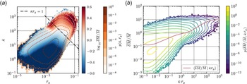


 Open access