


1. Introduction
Freezing of interstitial water in sediments commonly occurs in subaerial and subglacial environments, contributing to effects such as frost heave, needle ice and the transport of subglacial debris (Hemming Reference Hemming2004; Dash, Rempel & Wettlaufer Reference Dash, Rempel and Wettlaufer2006; Wettlaufer & Worster Reference Wettlaufer and Worster2006). Through multiple cycles of freeze and thaw in high-latitude environments, sediment patterns can develop such as the Arctic stone circles (Kessler & Werner Reference Kessler and Werner2003). In this paper, we consider the thermodynamical and fluid dynamical processes that occur as water freezes in a porous medium. We describe the melting and freezing processes using an enthalpy formulation, which facilitates our numerical method as we avoid tracking phase change interfaces. The enthalpy formulation also elucidates the role of the frozen fringe as a mushy zone of ice- and water-saturated sediments. Our treatment is general enough to apply in a variety of industrial and environmental contexts (e.g. Deville et al. Reference Deville, Saiz, Nalla and Tomsia2006) where interstitial freezing occurs, yet here we focus primarily on geophysical applications.
Consider frost heave, the common freeze/thaw phenomenon that takes place throughout high latitudes. As water held within sediments freezes, horizontally continuous, sediment-free ice lenses can form. These ice lenses cleave the sediment and expand, causing vertical displacement of the ground surface. Such surface displacement causes significant damage to infrastructure at high latitudes and is due to the growth of distinct ice lenses within the soil rather than the water density change on freezing. Taber (Reference Taber1930) demonstrated this fact by freezing a sediment pack saturated with benzene, which contracts on solidification; the benzene produced significant heave through the expansion of discrete solid lenses.
Early models for frost heave relied on surface tension to draw water to the lowest ice lens, i.e. the so-called ‘primary model for frost heave’ (Miller Reference Miller1978). This model suffers from several deficiencies, most importantly that surface tension acts tangential to the ice surface and cannot provide the upward force to drive heave. In addition, there is no mechanism to form distinct ice lenses in primary heave, which led O'Neill & Miller (Reference O'Neill and Miller1985) to derive the ‘secondary model of frost heave,’ wherein a zone of partially ice saturated sediment extends below the lowest ice lens (i.e. a frozen fringe; for reviews see Rempel Reference Rempel2010; Peppin & Style Reference Peppin and Style2013). Fowler & Krantz (Reference Fowler and Krantz1994) clarified the mathematical model for secondary frost heave and analysed an asymptotically reduced form of the model. Rempel, Wettlaufer & Worster (Reference Rempel, Wettlaufer and Worster2004) highlighted the role of premelting at the interface between ice and sediment grains. The disjoining pressure across the liquid between ice and sediment grains relates the local melting temperature to the vertical force balance. Fowler & Krantz (Reference Fowler and Krantz1994), on the other hand, choose the liquid pressure to be given as a function of soil water content as set by surface tension, reminiscent of a primary frost heave model. In what follows, we build on the Rempel et al. (Reference Rempel, Wettlaufer and Worster2004) formulation, highlighting an alternate derivation, writing out the equations, and systematically reducing the equations asymptotically, similar to Fowler & Krantz (Reference Fowler and Krantz1994).
Field observations show that several metres of frozen sediment are commonly attached to the base of glaciers, motivating efforts to understand alternative entrainment mechanisms that include glaciohydraulic supercooling (e.g. Röthlisberger & Lang Reference Röthlisberger and Lang1987; Lawson et al. Reference Lawson, Strasser, Evenson, Alley, Larson and Arcone1998; Creyts, Clarke & Church Reference Creyts, Clarke and Church2013) and frost heave. In the fastest flowing reaches of glaciers and ice sheets, sliding dominates glacier motion and the rate of sliding is tied to the temperature and water pressure at the glacier base: the same factors that control the growth of a frozen fringe. Rempel (Reference Rempel2008) treats the overlying glacier as a large lowest ice lens and predicts metre-scale frozen fringes below glaciers for typical parameters, in line with observations, while not accounting for the potential of initiating new ice lenses.
Anderson & Worster (Reference Anderson and Worster2012, Reference Anderson and Worster2014) analysed freezing colloid suspensions through directional solidification experiments with aqueous suspensions of alumina particles. Anderson & Worster (Reference Anderson and Worster2014) developed a model extending from the Rempel et al. (Reference Rempel, Wettlaufer and Worster2004) framework to include compaction and cohesion of the colloid suspension. The model of Anderson & Worster (Reference Anderson and Worster2014) assumes a steady-state linear temperature profile throughout the experiment and boils down to a system of ordinary differential equations for the location of the compaction front and frozen fringe extent, reminiscent of Fowler & Noon (Reference Fowler and Noon1993). Based on their model, Anderson & Worster (Reference Anderson and Worster2014) described a regime diagram showing the three primary freezing regimes observed in their experiments: periodic ice lenses, disordered ice lenses and periodic ice banding. Further work on solidification in colloidal suspensions has identified mechanisms of ice lens formation that are seeded by vertical dendritic growth into anomalously large pores that subsequently extend as propagating horizontal cracks, displacing particles to either side as they extend and develop into lenses (Style et al. Reference Style, Peppin, Cocks and Wettlaufer2011; Style & Peppin Reference Style and Peppin2012; Peppin Reference Peppin2020). By designing experiments that use heat exchangers to impose a desired, fixed temperature gradient, attention is focused on the mechanical interactions within these ice–liquid–colloid systems, justifying model treatments that ignore energy balance constraints despite the large role that latent heat plays in natural systems.
Frozen fringes and freeze–thaw cycles are inherently problems of phase change and partial melting. In these types of problems, it can be valuable to solve the energy conservation equation in an enthalpy form rather than for the temperature to avoid explicitly tracking phase change interfaces. The enthalpy (i.e. sum of the sensible and latent heat) accommodates the phase change, which facilitates numerical solutions. From sea ice (Katz & Worster Reference Katz and Worster2008), permafrost (Clow Reference Clow2018) and meltwater percolation through snow (Meyer & Hewitt Reference Meyer and Hewitt2017) to industrial processes (Voller & Prakash Reference Voller and Prakash1987), the enthalpy approach to phase change problems is useful for many applications. Enthalpy methods have been used extensively for polythermal glaciers, where part of the glacier is below the melting point and the rest of the glacier is at the melting point, i.e. temperate ice (Aschwanden et al. Reference Aschwanden, Bueler, Khroulev and Blatter2012; Schoof & Hewitt Reference Schoof and Hewitt2016; Meyer & Minchew Reference Meyer and Minchew2018). Here we use the enthalpy method to solve for energy conservation within a frozen fringe. Our thermomechanical model of a frozen fringe is more general than previous treatments. We use the enthalpy method numerical framework, which allows us to avoid the interface tracking issues of Rempel (Reference Rempel2007, Reference Rempel2008). We determine the local temperature from the enthalpy as opposed to using the constant temperature gradient models of Rempel et al. (Reference Rempel, Wettlaufer and Worster2004) and Anderson & Worster (Reference Anderson and Worster2014). Writing out the enthalpy method, we lay down the foundation for generalising the model to two- and three-dimensional versions in the future. We write out the full equations for mass, momentum and energy conservation as well as the boundary conditions. We then systematically scale the equations, allowing us to identify the important non-dimensional groups, neglect terms that are small and justify the idealisations used in Rempel et al. (Reference Rempel, Wettlaufer and Worster2004).
In this paper, we focus on the conditions relevant for subaerial frost heave and subglacial environments. Although numerous treatments of frost heave exist in the literature (e.g. Fowler & Krantz Reference Fowler and Krantz1994; Rempel et al. Reference Rempel, Wettlaufer and Worster2004; Style & Peppin Reference Style and Peppin2012), here we derive our model from scratch for completeness and clarity. In § 2, we start by writing down mass, momentum and energy conservation equations for a frozen fringe. Then, we non-dimensionalise and systematically reduce the equations by exploiting the small density difference between ice and water as well as the large latent heat of fusion upon freezing water (i.e. a large Stefan number). We solve our reduced model using an enthalpy method, where phase-change boundaries are determined implicitly on a fixed grid. In § 3, we demonstrate the results of our enthalpy model. We analyse a steady-state frozen fringe thickness in melting and balanced thermodynamic conditions in both a semi-analytical model and an enthalpy framework. Then, we examine the local effective pressure for melting and freezing conditions, highlighting ice lens formation. Lastly, we show the formation of periodic ice lenses and map out the different behaviour in a regime diagram for the heave rate and effective pressure. Finally, we offer conclusions and discuss future directions in § 4. The advances in this paper are (i) a systematic scaling of the model, which is not presented elsewhere, (ii) a numerical method that generalises to higher dimensions and (iii) a calculation of ice lens initiation and spacing, which we compare with laboratory experiments.
2. Model
Inside the frozen fringe, which is shown schematically in figure 1, we define a coordinate system that is fixed with respect to the immobile, water-saturated sediment below, with  $z$ vertical, $x$ the lateral coordinate and $y$ pointing into the page. We label the deepest extent of the fringe as $z=z_f$ and the top of the fringe as $z=z_{\ell }$, or equivalently $z_{\ell } = z_f+h$, where $h$ is the fringe thickness.
Schematic of the a frozen fringe system: (a) components including the lowermost ice lens or the bottom of a glacier, the frozen fringe and the unfrozen porous mixture of water-saturated sediments (after Rempel et al. Reference Rempel, Wettlaufer and Worster2004; Anderson & Worster Reference Anderson and Worster2014); (b) surface integral path  $\varGamma$ and inward-pointing normal vector ${\rm d}\boldsymbol {\varGamma }$; (c) volume integral domain $\varOmega$ with the outward-pointing normal vector ${\rm d}\boldsymbol {\varOmega }$.

2.1. Mass conservation
The frozen fringe is partitioned into three components: ice, water and sediment. The porosity  $\phi$ denotes the volume of voids (i.e. ice and water) within a representative control volume. The fraction of the voids that is taken up by ice is the ice saturation $S$. Mass conservation for sediment, ice and water implies that
 $$\begin{gather} \frac{\partial{\left[\rho_s(1-\phi)\right]}}{\partial{t}} + \boldsymbol{\nabla}\boldsymbol{\cdot} \left[ \rho_s (1-\phi) \boldsymbol{V_{s}}\right] = 0,\quad (\mbox{sediment}) \end{gather}$$
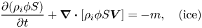 $$\begin{gather}\frac{\partial{\left(\rho_i\phi S\right)}}{\partial{t}} + \boldsymbol{\nabla}\boldsymbol{\cdot} \left[ \rho_i\phi S \boldsymbol{V}\right] =-m,\quad (\mbox{ice}) \end{gather}$$
 $$\begin{gather}\frac{\partial{\left[\rho_w\phi (1-S)\right]}}{\partial{t}} + \boldsymbol{\nabla}\boldsymbol{\cdot} \left[ \rho_w\phi \left(1-S\right) \boldsymbol{U}\right] = m,\quad (\mbox{water}) \end{gather}$$
where  $m$ is the rate at which ice (density $\rho _i$) is melted, i.e. converted into liquid water (density $\rho _w$), $\boldsymbol {V}$ is the speed at which the ice moves through the fringe due to heaving at the ice lens above the fringe and $\boldsymbol {V_{s}}$ is the sediment (density $\rho _s$) velocity. Here we treat the sediment, ice and water densities as constants, i.e. independent of space and time, so that each component is incompressible. The water flux through the fringe is $\boldsymbol {U}$, which is given by Darcy's law as
 \begin{equation} \phi \left(1-S\right) \boldsymbol{U} =-\frac{k}{\mu} \left[\boldsymbol{\nabla}p_w+\rho_w g \boldsymbol{k}\right], \end{equation}
where the permeability  $k$ depends on the ice saturation as well as the porosity $\phi$ and other properties of the sediment matrix. Here $g$ is the acceleration due to gravity and $\boldsymbol {k}$ is the unit vector in the
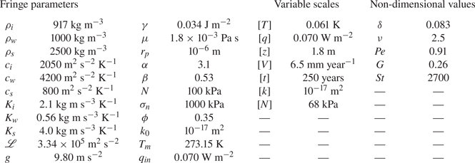
  $z$-direction. Values for all of the parameters are given in table 1.
Table of parameters for frozen fringe.
In this paper, we assume that the porosity  $\phi$ is constant throughout the fringe. There may be significant compaction below both the frozen fringe and in its interior due to the reduced water pressure as the lens pulls in water to freeze (Fowler & Noon Reference Fowler and Noon1999; Anderson & Worster Reference Anderson and Worster2012, Reference Anderson and Worster2014). We neglect such complications for now and take the entire sediment pack to maintain a constant porosity $\phi$ that jumps to $\phi =1$ at ice lenses. A new ice lens forms when the force between sediment grains reaches zero, as described in the next section.
2.2. Force balance
The force balance within the fringe is composed of three components: the weight of the material above and within the fringe, the water pressure within and below the fringe, as well as the thermomolecular force between sediment grains and interstitial ice, which acts across a thin film of premelted water (Dash et al. Reference Dash, Rempel and Wettlaufer2006). Integrating these components over the surface area of the fringe gives
 \begin{equation} \int_{\varGamma}{p_i \boldsymbol{n}\,{\rm d}\varGamma} = \int_{\varGamma}{\left(\,p_i - p_w\right) \boldsymbol{n}\,{\rm d}\varGamma} +\int_{\varGamma}{p_w \boldsymbol{n}\,{\rm d}\varGamma},\end{equation}
in which  $p_i$ is the isotropic ice pressure (i.e. local normal stress) at the ice–water interface within the fringe, $p_w$ is the water pressure at the boundary and $\boldsymbol {n}$ is the inward-pointing unit normal to the boundary $\varGamma$ (cf. figure 1). The difference between the ice and water pressure, i.e. the first term on the right-hand side of (2.5), is balanced by a thermomolecular force (Rempel, Wettlaufer & Worster Reference Rempel, Wettlaufer and Worster2001; Rempel et al. Reference Rempel, Wettlaufer and Worster2004; Wettlaufer & Worster Reference Wettlaufer and Worster2006).
We convert these surface integrals over  $\varGamma$ to volume integrals over the unfrozen component of the fringe $\varOmega$. We construct a closed surface by adding surface integrals with flat surfaces at $z_f$ and $z$, as shown schematically in figure 1. That is, for a generic pressure field $p$, we have the integrals
 \begin{equation} \int_{\varOmega}\boldsymbol{\nabla} p\,{\rm d}\varOmega = \int_{\varGamma}p \boldsymbol{n}\,{\rm d}\varGamma + \int_{\varGamma_z}p \boldsymbol{n}\,{\rm d}\varGamma + \int_{\varGamma_{z_f}}p \boldsymbol{n}\,{\rm d}\varGamma,\end{equation}
where  $\boldsymbol {n}$ is the outward-pointing normal for the volume $\varOmega$. In other words, $\boldsymbol {n}=\boldsymbol {k}$ on the upper cap at $z$, the lowest ice lens, and $\boldsymbol {n}=-\boldsymbol {k}$ on the lower cap at the bottom of the fringe $z_{f}$, where $\boldsymbol {k}$ is the unit vector in the $z$-direction.
We take the surface  $\varGamma _z$ to be the ice boundary at some height $z$, which we can write $|\varGamma _z| = (1-\phi S)A$ where $A$ is the cross-sectional area. This surface has the two limits of $|\varGamma _{z_{\ell }}| = 0$ at the bottom boundary of the lowest active ice lens ( $\phi =1$, $S=1$) and $|\varGamma _{z_{f}}| = A$ at the bottom of the fringe ( $S=0$). For this reason, no upper cap is necessary when integrating across the entire fringe, and (2.6) reduces to
 \begin{equation} \int_{\varOmega}\boldsymbol{\nabla} p\,{\rm d}\varOmega = \int_{\varGamma}p \boldsymbol{n}\,{\rm d}\varGamma + \int_{\varGamma_{z_f}}p \boldsymbol{n}\,{\rm d}\varGamma. \end{equation}
 We assume that water flow through ice-saturated porous fringe is governed by Darcy's law and that the water pressure varies only on a length scale set by the fringe and not on the scale of individual grains. This assumption allows us to define the water pressure throughout the volume  $\varOmega$, even though part of the domain is filled with ice and sediment. Crucially, we follow Rempel et al. (Reference Rempel, Wettlaufer and Worster2004) and assume that the microscale pressure is the homogenised pore pressure given by Darcy's law. In other words, we treat the water pressure in the thin films between sediment and ice as well as the water pressure in the pore throats between sediment grains as determined by Darcy's law, which is a key difference between Fowler & Krantz (Reference Fowler and Krantz1994) and Rempel et al. (Reference Rempel, Wettlaufer and Worster2004).
At this stage, we restrict our focus to a one-dimensional water pressure that only depends on the vertical coordinate  $z$ and assume that there are no transverse pressure gradients. Therefore, inserting the water pressure $p_w$ into (2.6), we find that
 \begin{equation} \int_{\varGamma}p_w \boldsymbol{n}\,{\rm d}\varGamma = A\left[ \int_{z_f}^{z}(1-\phi S)\frac{\partial{p_w}}{\partial{z'}}\,{\rm d}z' - (1-\phi S)p_w(z) + p_w(z_f)\right]\boldsymbol{k},\end{equation}
where the porosity  $\phi$ and saturation $S$ also depend on the vertical coordinate $z$. Now integrating across the entire fringe from $z_f$ to $z_{\ell }$ gives
 \begin{equation} \int_{\varGamma}p_w \boldsymbol{n}\,{\rm d}\varGamma = A\left[ \int_{z_f}^{z_{\ell}}(1-\phi S)\frac{\partial{p_w}}{\partial{z'}}\,{\rm d}z' + p_w(z_f)\right]\boldsymbol{k}.\end{equation}
The analogous equation for  $p_i-p_w$ represents the thermomolecular contribution to the force balance (Rempel & Worster Reference Rempel and Worster1999; Rempel et al. Reference Rempel, Wettlaufer and Worster2004) and is given by
 \begin{equation} \int_{\varGamma}\left(\,p_i-p_w\right) \boldsymbol{n}\,{\rm d}\varGamma = A\left[ \int_{z_f}^{z_{\ell}}(1-\phi S)\frac{\partial{\left(\,p_i - p_w\right)}}{\partial{z'}}\,{\rm d}z' + p_i(z_f)-p_w(z_f)\right]\boldsymbol{k}.\end{equation}
 When integrated across the entire fringe, the water pressure and thermomolecular force balance the total normal stress  $\sigma _n$ at $z_f$ resulting from the weight of the overlying material (e.g. (2.5) and figure 1). With this in mind, we write
 \begin{equation} \int_{\varGamma}p_i \boldsymbol{n}\,{\rm d}\varGamma = \left\{\sigma_n - \int_{z_f}^{z_{\ell}}\left[\rho_s g (1-\phi) + \rho_w g \phi (1-S)\right]{\rm d}z' \right\} A \boldsymbol{k},\end{equation}
where we have included the weight of fringe material as the integral over each constituent.
We now combine the equations for ice (2.11), water (2.9) and thermomolecular pressure (2.10) as well as include the effects of gravity (2.11) to arrive at
 \begin{align} \sigma_n &= \int_{z_f}^{z_{\ell}}\left[\rho_s g (1-\phi) + \rho_w g \phi (1-S)\right]{\rm d}z' \nonumber\\ &\quad +\int_{z_f}^{z_{\ell}}(1-\phi S)\frac{\partial{\left(\,p_i-p_w\right)}}{\partial{z'}}{\rm d}z' + p_i(z_f) -p_w(z_f) \nonumber\\ &\quad +\int_{z_f}^{z_{\ell}}(1-\phi S)\frac{\partial{p_w}}{\partial{z'}}\,{\rm d}z' + p_w(z_f). \end{align}
We define the effective pressure at the base of the fringe  $N$ as the total normal stress $\sigma _n$ at $z_f$ supported by the fringe less the water pressure at the base of the fringe $p_w(z_f)$ so that
 \begin{equation} N = \sigma_n - p_w(z_f), \end{equation}
and
 \begin{align} N &= \int_{z_f}^{z_{\ell}}\left[\rho_s g (1-\phi) + \rho_w g \phi (1-S)\right]{\rm d}z' \nonumber\\ &\quad +\int_{z_f}^{z_{\ell}}(1-\phi S)\frac{\partial{\left(\,p_i-p_w\right)}}{\partial{z'}}\,{\rm d}z' + p_i(z_f) -p_w(z_f) + \int_{z_f}^{z_{\ell}}{(1-\phi S)\frac{\partial{p_w}}{\partial{z'}}\,{\rm d}z'}. \end{align}
We recognise  $N$ as the load supported by contacts between sediment grains at $z_f$.
In addition, we define the local effective pressure  $N_{loc}(z)$ as the portion of the overlying load that is supported at a height $z$ by sediment grain contacts. The rest of the overlying load is supported by thermomolecular forces or water pressure acting on the ice fringe below the height $z$ as well as water pressure at height $z$. The thermomolecular and water pressure contributions from below $z$ are given as
 \begin{align} \int_{\varGamma}p_i
\boldsymbol{n}\,{\rm d}\varGamma & =
A\left\{\int_{z_f}^{z}\left[\rho_s g (1-\phi) + \rho_w g
\phi (1-S) \right]{\rm d}z'\right. \nonumber\\ &\quad
\left.+ \int_{z_f}^{z}(1-\phi
S)\frac{\partial{(\,p_i-p_w)}}{\partial{z'}}\,{\rm d}z' +
p_i(z_f)-p_w(z_f) - (1-\phi S)\left[ p_i(z)-p_w(z) \right]
\right. \nonumber\\ &\quad \left. + \int_{z_f}^{z}(1-\phi
S)\frac{\partial{p_w}}{\partial{z'}}\,{\rm d}z' + p_w(z_f)
- (1-\phi S)p_w(z) \right\}\boldsymbol{k}.
\end{align}
\begin{align} \int_{\varGamma}p_i
\boldsymbol{n}\,{\rm d}\varGamma & =
A\left\{\int_{z_f}^{z}\left[\rho_s g (1-\phi) + \rho_w g
\phi (1-S) \right]{\rm d}z'\right. \nonumber\\ &\quad
\left.+ \int_{z_f}^{z}(1-\phi
S)\frac{\partial{(\,p_i-p_w)}}{\partial{z'}}\,{\rm d}z' +
p_i(z_f)-p_w(z_f) - (1-\phi S)\left[ p_i(z)-p_w(z) \right]
\right. \nonumber\\ &\quad \left. + \int_{z_f}^{z}(1-\phi
S)\frac{\partial{p_w}}{\partial{z'}}\,{\rm d}z' + p_w(z_f)
- (1-\phi S)p_w(z) \right\}\boldsymbol{k}.
\end{align}
We assume that sediment grains have infinitesimal contacts and, therefore, the water pressure at the height  $z$ supports the force $A(1-\phi S)p_w(z)\boldsymbol {k}$, which excludes the areas occupied by ice. The total force supported by grain contacts at a height $z$ is the overburden $\sigma _n$ minus both (2.15) and the water pressure at $z$. Thus, we can write the effective pressure $N_{loc}(z)$ as
 \begin{align} N_{loc}(z) &= N - \left\{\int_{z_f}^{z}\left[\rho_s g (1-\phi) + \rho_w g \phi (1-S)\right]{\rm d}z' \right. \nonumber\\ &\quad \left.-\int_{z_f}^{z}\phi S\frac{\partial{(\,p_i-p_w)}}{\partial{z'}}\,{\rm d}z' + \phi S\left[ p_i(z)-p_w(z) \right] + \int_{z_f}^{z}(1-\phi S)\frac{\partial{p_w}}{\partial{z'}}\,{\rm d}z' \right\}. \end{align}
A new ice lens initiates at the height  $z_n$ where the local effective pressure is zero, i.e. $N_{loc}(z_n) = 0$, as there is no longer any force on the sediment grains (O'Neill & Miller Reference O'Neill and Miller1985; Rempel et al. Reference Rempel, Wettlaufer and Worster2004; Anderson & Worster Reference Anderson and Worster2014). We do not consider geometric supercooling and ice-lens initiation through crack propagation (Style et al. Reference Style, Peppin, Cocks and Wettlaufer2011), but our model is flexible enough to incorporate these effects in the future. We treat the effective pressure at the bottom of the fringe $N$ as an input to the model that is determined by groundwater hydrology or subglacial drainage (e.g. Schoof Reference Schoof2010).
2.3. Generalised Clausius–Clapeyron and Gibbs–Thomson
The pressure difference between ice and water is related to temperature through the generalised Clausius–Clapeyron equation, which in its linearised form is given by
 \begin{equation} p_i - p_w = \rho_i \mathscr{L} \frac{T_m-T}{T_m} + \left( p_m - p_w\right) \frac{\rho_w-\rho_i}{\rho_w}, \end{equation}
where the bulk melting temperature at the reference pressure  $p_m$ is $T_m$, the specific latent heat of fusion for ice is $\mathscr {L}$ and the densities of ice and water are given as $\rho _i$ and $\rho _w$, respectively (Worster & Wettlaufer Reference Worster and Wettlaufer1999; Worster Reference Worster2000; Clarke Reference Clarke2005). We choose the reference pressure to be the overburden $\sigma _n$, so that at the bottom of the fringe $z=z_f$, we have
 \begin{equation} p_i(z_f) - p_w(z_f) = \rho_i \mathscr{L} \frac{T_m-T}{T_m} + \frac{\rho_w-\rho_i}{\rho_w}N, \end{equation}
and in the interior of the fringe, we have
 \begin{equation} p_i(z) - p_w(z) = \rho_i \mathscr{L} \frac{T_m-T}{T_m} + \frac{\rho_w-\rho_i}{\rho_w}\left[N + p_w(z_f) - p_w(z)\right].\end{equation}
Note that in this formulation changes to  $\sigma _n$ affect the value of $N$ and $T_m$.
At the bottom of the fringe, the ice is in contact with water in between pore throats, as shown in the schematic in figure 1. The curvature induced by the space between sediment grains, leads to a difference in the pressure in ice and water phases due to the Gibbs–Thomson effect (Worster Reference Worster2000), which is given by
 \begin{equation} p_i(z_f) - p_w(z_f) = \gamma \kappa, \end{equation}
where  $\gamma$ is the ice–water surface energy and $\kappa$ is the curvature of the ice–water interface. Moreover, the curvature $\kappa$ at the bottom of the fringe is related to the radius of curvature for sediment pore throats $r_p$ as $\kappa =2/r_p$. The critical effective pressure required to overcome the pore throat curvature is given by the Gibbs–Thomson effect and defined by the right-hand side of (2.20), i.e.
 \begin{equation} N_c = \frac{2\gamma}{r_p} \end{equation}
(e.g. Fowler Reference Fowler1997; Rempel Reference Rempel2008; Meyer, Downey & Rempel Reference Meyer, Downey and Rempel2018).
Combining the generalised Claussius–Clapeyron equation (2.19) and the Gibbs–Thomson effect (2.20) at the bottom of the fringe, we can relate the curvature induced by pore throats to the temperature at the interface, which is given by
 \begin{equation} \rho_i \mathscr{L} \frac{T_m-T}{T_m} = N_c - \frac{\rho_w-\rho_i}{\rho_w}N. \end{equation}
The contribution from surface energy on the right-hand side typically dominates the term proportional to the density difference, because ice and water densities differ by less than 10 %. Therefore, it is useful to define the undercooling temperature  $T_f$ that supports this balance as
 \begin{equation} T_f = T_m-\frac{N_c T_m}{\rho_i \mathscr{L}}, \end{equation}
which allows us to write (2.22) as
 \begin{equation} T(z_f) = T_f + \frac{\left(\rho_w-\rho_i\right)N}{\rho_i \rho_w \mathscr{L}}T_m. \end{equation}
Rempel (Reference Rempel2008) dropped the second term on the right arguing that it is small, which is consistent with the dominant balance for the small difference between ice and water densities. We, however, keep all terms for now and reduce the model systematically in § 2.7.2.
At this stage, we can now insert the generalised Clausius–Clapeyron equation (2.19) and the Gibbs–Thomson effect (2.20) into the effective pressure integrals (2.14) and (2.16). The effective pressure at the bottom of the fringe  $N$ is then
 \begin{align} N &= N_c+\int_{z_f}^{z_{\ell}}\left[\rho_s g (1-\phi) + \rho_w g \phi (1-S) \right]{\rm d}z'\nonumber\\ &\quad - \int_{z_f}^{z_{\ell}}(1-\phi S)\left[\frac{\rho_i \mathscr{L}}{T_m}\frac{\partial{T}}{\partial{z'}}-\frac{\rho_i}{\rho_w}\frac{\partial{p_w}}{\partial{z'}}\right]{\rm d}z'. \end{align}
In the interior of the fringe, the local effective pressure is given by
 \begin{align} N_{loc}(z) &= N - \left\{\int_{z_f}^{z}\left[\rho_s g (1-\phi) + \rho_w g \phi (1-S)\right]{\rm d}z' +\frac{\rho_i \mathscr{L}}{T_m} \int_{z_f}^{z}{\phi S \frac{\partial{T}}{\partial{z'}} \,{\rm d}z'} \right. \nonumber\\ &\quad + \phi S\left[ \rho_i \mathscr{L} \frac{T_m-T}{T_m} + \frac{\rho_w-\rho_i}{\rho_w}\left[N + p_w(z_f) - p_w(z)\right] \right] \nonumber\\ &\quad\left. +\int_{z_f}^{z}\left(1-\frac{\rho_i}{\rho_w} \phi S \right)\frac{\partial{p_w}}{\partial{z'}}\,{\rm d}z' \right\}, \end{align}
which connects the local pressure and temperature.
If there is not a fringe, the development of the force balance at the base of the fringe still holds, except that  $z_{f} = z_{\ell }$ and the integrals vanish. In addition, the curvature at the bottom of the ice is no longer $\kappa = 2/r_p$ and so the effective pressure is given by
 \begin{equation} N = p_i(z_f) - p_w(z_f) < N_c, \end{equation}
while the temperature at bottom of the ice is given by
 \begin{equation} T(z_f) = T_m - \frac{T_m}{\rho_w \mathscr{L}}N, \end{equation}
which is modulated by the effective pressure.
2.4. Energy conservation
Mass exchange between the liquid and solid phases within the fringe leads to changes in ice saturation. Conservation of energy determines the temperature and phase change within the fringe and can be expressed in terms of the enthalpy,  $H_\alpha$. For the constituents $\alpha$ that make up the fringe, sediment ( $s$), ice ( $i$) and water ( $w$), conservation of energy in enthalpy form is given as
 \begin{align} &\int_{\varOmega}{\frac{\partial{}}{\partial{t}} \left[ (1-\phi)\rho_s H_s + \phi S\rho_{i}H_{i} + \phi (1-S) \rho_{w}H_{w}\right] {\rm d}\varOmega} \nonumber\\ &\quad =\int_{\varGamma}{ \left\{ -\phi S \rho_i H_i \boldsymbol{V} - \phi \left( 1- S\right) \rho_{w}H_{w}\boldsymbol{U} - \left( 1- \phi \right)\rho_{s}H_{s}\boldsymbol{V}_s + K_e\boldsymbol{\nabla}T\right\}\boldsymbol{\cdot} {\rm d}\boldsymbol{\varGamma}}, \end{align}
where  $K_e$ is the effective thermal conductivity (Appendix B of Rempel Reference Rempel2008), which can be represented as
 \begin{equation} K_e = K_s^{(1-\phi)}K_i^{S\phi}K_w^{(1-S)\phi},\end{equation}
for randomly packed fringe constituents, sediment  $K_s$, ice $K_i$ and water $K_w$ (Clauser & Huenges Reference Clauser and Huenges1995). Using the divergence theorem, we can write (2.29) as
 \begin{align} &\frac{\partial{}}{\partial{t}}\left[ (1-\phi)\rho_s H_s + \phi S\rho_{i}H_{i} + \phi (1-S) \rho_{w}H_{w}\right] \nonumber\\ &\quad =-\boldsymbol{\nabla}\boldsymbol{\cdot} \left\{\phi S \rho_i H_i \boldsymbol{V} + \phi \left( 1- S\right) \rho_{w}H_{w}\boldsymbol{U} + \left( 1- \phi \right)\rho_{s}H_{s}\boldsymbol{V}_s \right\} + \boldsymbol{\nabla}\boldsymbol{\cdot}\left( K_e \boldsymbol{\nabla}T\right). \end{align}
We define the difference between the water flux  $\boldsymbol {U}$ and the heave rate $\boldsymbol {V}$ as $\boldsymbol {u}$, i.e.
 \begin{equation} \boldsymbol{u} = \boldsymbol{U}-\boldsymbol{V}, \end{equation}
which will typically be small as it is the flow of water that allows for heave. Water flow is given by Darcy's law (2.4) as
 \begin{equation} \phi (1-S) \boldsymbol{u} =-\phi (1-S) \boldsymbol{V} - \frac{k(S)}{\mu}\left(\frac{\partial{p_w}}{\partial{z}}+\rho_w g\right). \end{equation}
Thus, we combine the mass conservation equations (2.2) and (2.3) as
 \begin{align} \frac{\partial{}}{\partial{t}}\left[\phi S\rho_i + \phi (1-S)\rho_{w}\right] + \boldsymbol{\nabla} \boldsymbol{\cdot} \left\{\left[\phi S\rho_i + \phi (1-S)\rho_{w}\right]\boldsymbol{V}\right\} + \boldsymbol{\nabla}\boldsymbol{\cdot}\left[\rho_w \phi \left(1-S\right) \boldsymbol{u}\right] = 0,\end{align}
which allows us to define the total water  $W$ (e.g. Meyer & Hewitt Reference Meyer and Hewitt2017) that is given by
 \begin{equation} W = \phi S\rho_i + \phi (1-S) \rho_{w}, \end{equation}
so that in the rigid-ice limit with  $\boldsymbol {\nabla } \boldsymbol {\cdot } \boldsymbol {V}=0$ where the heave rate is spatially independent, mass conservation (2.34) can be written succinctly as
 \begin{equation} \frac{\partial{W}}{\partial{t}}+ \boldsymbol{V}\boldsymbol{\cdot}\boldsymbol{\nabla}W + \boldsymbol{\nabla}\boldsymbol{\cdot} \left[ \rho_w \phi \left(1-S\right) \boldsymbol{u}\right] = 0.\end{equation}
 Similarly, for conservation of energy we can define the water enthalpy  $H$ as
 \begin{equation} H = H_0+\phi S\rho_{i}H_{i} + \phi (1-S) \rho_{w}H_{w},\end{equation}
which is specified up to a constant, reference enthalpy  $H_0$, which we choose to make $H=0$ at $T=T_f$. Thus, (2.31) reduces to
 \begin{align} &\frac{\partial{H}}{\partial{t}}+\boldsymbol{V}\boldsymbol{\cdot}\boldsymbol{\nabla}H +\frac{\partial{}}{\partial{t}}\left[ (1-\phi)\rho_s H_s\right] + \boldsymbol{\nabla}\boldsymbol{\cdot}\left[\phi \left( 1- S\right) \rho_{w}H_{w}\boldsymbol{u} + \left( 1- \phi\right) \rho_{s}H_{s}\boldsymbol{V}_s \right]\nonumber\\ &\quad = \boldsymbol{\nabla}\boldsymbol{\cdot}\left( K_e \boldsymbol{\nabla}T\right). \end{align}
Using the fact that the latent heat  $\mathscr {L}$ is equal to the difference between the liquid and ice enthalpies, i.e. $\mathscr {L} = H_w - H_i$, we find that
 \begin{equation} H = H_0+WH_{i} +\rho_w \mathscr{L} \phi (1-S), \end{equation}
which is a sum of sensible and latent heat contributions to energy. We leave (2.38) in enthalpy form to facilitate the description of the numerical method. For an incompressible medium, the enthalpy  $H_\alpha$ is equivalent to a change in temperature, i.e. ${\rm d}H_\alpha = c_\alpha \,{\rm d}T$, where $c_\alpha$ is the specific heat capacity with $\alpha$ representing ice, liquid or sediments. Thus, the enthalpy can be related to temperature as
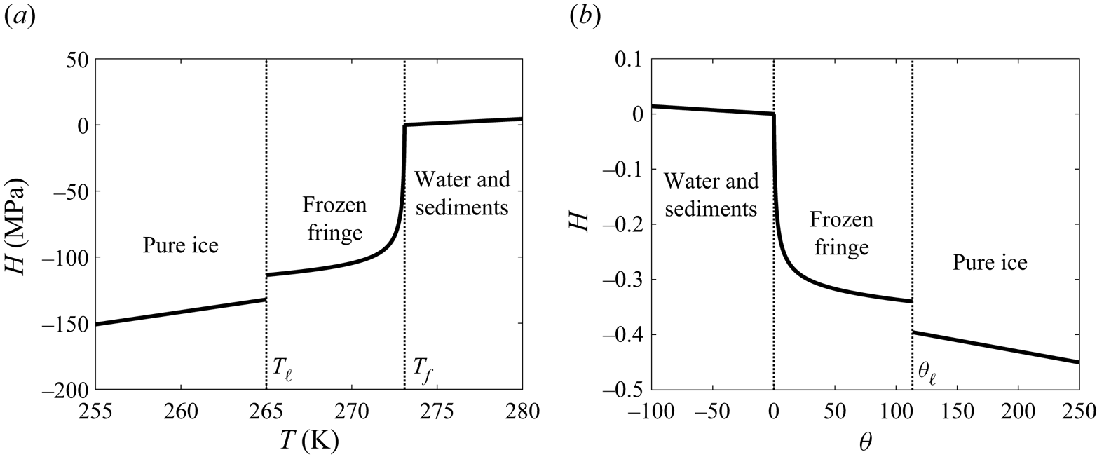
 \begin{equation} H = \left \{\begin{array}{@{}lll} \rho_i c_i \left(T - T_f\right)-\rho_w \mathscr{L} & T < T_\ell & \mbox{(pure ice)}\\ W c_i \left(T - T_f\right)-\rho_w \mathscr{L} \phi S & T_\ell \le T < T_f & \mbox{(frozen fringe)}\\ \rho_w c_i \phi \left(T - T_f\right) & T_f \le T & \mbox{(water and sediments)}, \end{array}\right. \end{equation}
which we show schematically in figure 2. Our choice of reference enthalpy implies that  $H_0 = -\rho _w \phi \mathscr {L}$. As we describe in the next section, the ice saturation in the fringe is a function of the temperature.
Schematic for the enthalpy H below an ice lens. (a) Temperatures below  $T_\ell$ occur above the lowest ice lens; within the fringe, the temperature is tied to the ice saturation curve; and below the fringe, the water and sediment temperatures rise above $T_f$. (b) Non-dimensional version of (a) showing that the enthalpy is zero at $\theta =0$ and negative non-dimensional temperatures correspond to unfrozen water with positive enthalpy.
2.5. Constitutive relations for saturation and permeability
The ice saturation  $S$ and, therefore, the permeability $k$ of the frozen fringe depend on the local thermodynamics with the pressure difference between the phases controlled by the Gibbs–Thomson effect and interfacial premelting (Andersland & Ladanyi Reference Andersland and Ladanyi2004; Hansen-Goos & Wettlaufer Reference Hansen-Goos and Wettlaufer2010; Rempel Reference Rempel2012). Here we use the generalised Clausius–Claperyon relation to specify the ice saturation $S$ and permeability $k$ as functions of the local difference between ice pressure and water pressure. That is, we generalise the relationships used by Rempel (Reference Rempel2007, Reference Rempel2008) and define the function $\varXi$ as the ratio of the critical effective stress to the local pressure difference $p_i-p_w$, i.e.
 \begin{equation} \varXi = \frac{N_c}{p_i - p_w} = \frac{T_m - T_f}{T_m - T(z) + \dfrac{\left(\rho_w - \rho_i\right)T_m}{\rho_i \rho_w \mathscr{L}}\left(N_{loc} + p_w(z_f) - p_w(z) \right)}. \end{equation}
This reduces to the expression used by Rempel (Reference Rempel2007, Reference Rempel2008) if we ignore the density difference between ice and water. For now, we proceed with the definition in (2.41) and write the ice saturation and permeability as
 $$\begin{gather} S = 1 - \varXi^{\beta}, \end{gather}$$
 $$\begin{gather}k = k_0 \left(1 - S\right)^{\alpha/\beta}, \end{gather}$$
where the empirical exponents are  $\beta >0$ and $\alpha >\beta$ (typically $\alpha >1$; see Watanabe & Mizoguchi Reference Watanabe and Mizoguchi2002; Rempel Reference Rempel2008; Chen et al. Reference Chen, Mei, Irizarry and Rempel2020; Chen, Rempel & Mei Reference Chen, Rempel and Mei2021).
2.6. Boundary conditions
Now that we have specified the governing equations for enthalpy  $H$ and total water $W$, we describe the boundary conditions. At the top of the lowest fringe, i.e. $z=z_{\ell }$, a finite jump in saturation can occur as the ice lens is fully occupied by ice ( $\phi =1$ and $S=1$) whereas ice only partially saturates the interstices in the underlying fringe ( $\phi <1$ and $S<1$). Integrating mass and energy conservation across the jump at the lowest ice lens boundary gives the following conditions:
 $$\begin{gather} \left[W \boldsymbol{V} + \rho_w\phi \left(1-S\right) \boldsymbol{u}\right]_-^+ \boldsymbol{\cdot} \boldsymbol{n} = 0\quad \mbox{across}\ z=z_{\ell}, \end{gather}$$
 $$\begin{gather}\left[-K_e \boldsymbol{\nabla}T + H\boldsymbol{V} + \phi \left( 1- S\right) \rho_{w}H_{w}\boldsymbol{u} + \left( 1- \phi\right) \rho_{s}H_{s}\boldsymbol{V}_s\right]_-^+\boldsymbol{\cdot}\boldsymbol{n} = 0\quad \mbox{across}\ z=z_{\ell}. \end{gather}$$
Taking the heat flux into the ice lens and material above as  $q$, we can simplify these conditions to
 $$\begin{gather} \left[W \boldsymbol{V} + \rho_w\phi \left(1-S\right) \boldsymbol{u}\right]_-\boldsymbol{\cdot}\boldsymbol{n} = \rho_i \boldsymbol{V}\boldsymbol{\cdot}\boldsymbol{n}\quad \mbox{at}\ z=z_{\ell} \end{gather}$$
 $$\begin{gather}\left[-K_e \boldsymbol{\nabla}T + H\boldsymbol{V} + \phi \left( 1- S\right) \rho_{w}H_{w}\boldsymbol{u} + \left( 1- \phi\right) \rho_{s}H_{s}\boldsymbol{V}_s\right]_-\boldsymbol{\cdot}\boldsymbol{n} = \boldsymbol{q}\boldsymbol{\cdot}\boldsymbol{n}\quad \mbox{at}\ z=z_{\ell}, \end{gather}$$
where mass conservation implies that at the top of the fringe, all of the liquid water must freeze onto the lowest ice lens, and conservation of energy implies that all the heat that enters the fringe at the bottom must leave through the top. At the bottom of the fringe (or at any point below the fringe), we impose a conductive heat flux  $q$ which includes contributions from geothermal heat and friction from sliding, i.e.
 \begin{equation} \left.-K_e \boldsymbol{\nabla}T\right |^+\boldsymbol{\cdot}\boldsymbol{n} = q_{in} \quad \mbox{on}\ z=z_{f}, \end{equation}
which is the full heat flux as  $H=0$ at the base of the fringe (i.e. where we have chosen $H_0$ such that $H=0$ when $T=T_f$). The ice saturation transitions smoothly from $0\le S<1$ within the fringe to $S=0$ below the fringe and, therefore, no jump condition is required at $z=z_f$. The water pressure $p_w$ at the bottom of the fringe is set by the effective pressure $N$ and is given by
 \begin{equation} p_w = \sigma_n - N\quad \mbox{on}\ z=z_{f}. \end{equation}
2.7. Non-dimensionalisation
We now scale our model to find the dominant physical balances. For example, we write  $t = [t]t^{*}$ for the time $t$, where $[t]$ is the scale and $t^{*}$ is the non-dimensional variable. Proceeding in this way, we write all variables as
 \begin{align} \left.\begin{gathered} N = [N]N^{*},\quad p_w = \sigma_n - N + [N]p_w^{*},\quad T = T_f - [T]\theta,\quad K_e = K_i K^{*},\quad V = [V]V^{*} \\ z = [z]z^{*},\quad t= [t]t^{*},\quad k = [k]k^{*},\quad H = \rho_w \mathscr{L} H^{*},\quad W = \rho_w W^{*},\quad h = c_i [T] h^{*}, \end{gathered}\right\} \end{align}
and choose the scales for the variables based on the expected physical balances.
A scale for the effective pressure within the fringe is the threshold entry pressure, i.e.  $[N] = N_c$, and a scale for the heat flux into the fringe is the geothermal heat flux, i.e. $[q]=q_{in}$. We choose the temperature scale to be the temperature difference implied by premelting, i.e.
 \begin{equation} [N] = \frac{\rho_i \mathscr{L} [T]}{T_m}\longrightarrow [T] = \frac{T_m [N]}{\rho_i \mathscr{L}}. \end{equation}
A scale for the vertical distance  $[z]$ comes from the heat flux scale, i.e.
 \begin{equation} [q] = K_i\frac{[T]}{[z]} \longrightarrow [z] = K_i\frac{[T]}{[q]}. \end{equation}
The rate of heaving is determined by water percolation, so we choose
 \begin{equation} [V] = \frac{[k][N]}{\mu[z]}, \end{equation}
and time can be scaled for the solidification as
 \begin{equation} \frac{\rho_w \mathscr{L}}{[t]}=K_i \frac{[T]}{[z]^2} \longrightarrow [t]=\frac{\rho_w \mathscr{L}[z]^2}{K_i [T]}. \end{equation}
For the permeability, we choose the scale to be the prefactor as
 \begin{equation} [k] = k_0. \end{equation}
We also define the dimensionless variables
 \begin{equation} \delta = 1 -
\frac{\rho_i}{\rho_w},\quad \nu =
\frac{\rho_s}{\rho_w},\quad {\textit{Pe}} = \frac{[V][t]}{[z]},\quad
{\textit{G}} = \frac{\rho_w g [z]}{[N]},\quad {\textit{St}} = \frac{\mathscr{L}}{c_i
[T]},
\end{equation}
\begin{equation} \delta = 1 -
\frac{\rho_i}{\rho_w},\quad \nu =
\frac{\rho_s}{\rho_w},\quad {\textit{Pe}} = \frac{[V][t]}{[z]},\quad
{\textit{G}} = \frac{\rho_w g [z]}{[N]},\quad {\textit{St}} = \frac{\mathscr{L}}{c_i
[T]},
\end{equation}
where  $\delta$ is the scaled density difference, $\nu$ is the ratio of the sediment density to water density, ${\textit{Pe}}$ is the Péclet number, ${\textit{G}}$ is the ratio of gravitational hydrostatic pressure to infiltration pressure and ${\textit{St}}$ is the Stefan number.
2.7.1. Full model
We now write the model in non-dimensional variables and for concision, we drop the asterisks. Rewriting (2.25), the force balance across the fringe is
 \begin{align} N =1 + {\textit{G}}\int_{z_f}^{z_{\ell}}{\left[\nu (1-\phi) + \phi\left(1-S\right)\right]{\rm d}z'}+ \int_{z_f}^{z_{\ell}}\left( 1 - \phi S\right) \left[\frac{\partial{\theta}}{\partial{z'}}+ \left( 1-\delta\right) \frac{\partial{p_w}}{\partial{z'}}\right]{\rm d}z', \end{align}
if a fringe exists, or the effective pressure is constrained by  $N<1$ if there is not a fringe. The local effective pressure in the fringe is
 \begin{align} N_{loc}(z) &= N - \left\{{\textit{G}}\int_{z_f}^{z}\left[\nu (1-\phi) + \phi\left(1-S\right)\right]{\rm d}z' - \int_{z_f}^{z}\phi S \frac{\partial{\theta}}{\partial{z'}} \,{\rm d}z' \right. \nonumber\\ &\quad + \left. \phi S\left[1 + \theta+ \delta\left(N - p_w(z)\right)\right] + \int_{z_f}^{z}\left[1-\left( 1-\delta \right) \phi S \right]\frac{\partial{p_w}}{\partial{z'}}\,{\rm d}z' \right\}. \end{align}
The total water in the fringe is
 \begin{equation} W = \phi\left(1-\delta S\right), \end{equation}
and the enthalpy is
 \begin{align}
H &= \frac{1}{{\textit{St}}}WH_{i} - \phi S \nonumber\\
&= \left \{ {\begin{array}{@{}lll}
-(1-\delta)(\theta/{\textit{St}})-1 & \theta > 0 \& \phi=1 & \textrm{ (pure ice), }\\
-\phi (1-\delta S)(\theta/{\textit{St}})-\phi S & \theta > 0 & \textrm{ (frozen fringe), }\\
-\phi(\theta/{\textit{St}}) & \theta \le 0 & \textrm{ (water and sediments). }
\end{array}}\right.
\end{align}
\begin{align}
H &= \frac{1}{{\textit{St}}}WH_{i} - \phi S \nonumber\\
&= \left \{ {\begin{array}{@{}lll}
-(1-\delta)(\theta/{\textit{St}})-1 & \theta > 0 \& \phi=1 & \textrm{ (pure ice), }\\
-\phi (1-\delta S)(\theta/{\textit{St}})-\phi S & \theta > 0 & \textrm{ (frozen fringe), }\\
-\phi(\theta/{\textit{St}}) & \theta \le 0 & \textrm{ (water and sediments). }
\end{array}}\right.
\end{align}Non-dimensionalising (2.38) results in
 \begin{align}
&\frac{\partial{H}}{\partial{t}}+{\textit{Pe}}\boldsymbol{V}\boldsymbol{\cdot}\boldsymbol{\nabla}H
+\frac{\nu}{{\textit{St}}} \frac{\partial{}}{\partial{t}}\left[
(1-\phi) H_s\right] + \frac{{\textit{Pe}}}{{\textit{St}}}
\boldsymbol{\nabla}\boldsymbol{\cdot}\left[\phi \left( 1-
S\right) H_{w}\boldsymbol{u} + \nu (1-\phi) H_s
\boldsymbol{V}_s\right] \nonumber\\ &\quad
=-\boldsymbol{\nabla}\boldsymbol{\cdot}\left( K
\boldsymbol{\nabla}\theta\right).
\end{align}
\begin{align}
&\frac{\partial{H}}{\partial{t}}+{\textit{Pe}}\boldsymbol{V}\boldsymbol{\cdot}\boldsymbol{\nabla}H
+\frac{\nu}{{\textit{St}}} \frac{\partial{}}{\partial{t}}\left[
(1-\phi) H_s\right] + \frac{{\textit{Pe}}}{{\textit{St}}}
\boldsymbol{\nabla}\boldsymbol{\cdot}\left[\phi \left( 1-
S\right) H_{w}\boldsymbol{u} + \nu (1-\phi) H_s
\boldsymbol{V}_s\right] \nonumber\\ &\quad
=-\boldsymbol{\nabla}\boldsymbol{\cdot}\left( K
\boldsymbol{\nabla}\theta\right).
\end{align}
The scaled total water equation is given by
 \begin{equation} \frac{\partial{W}}{\partial{t}}+ {\textit{Pe}}\boldsymbol{V}\boldsymbol{\cdot}\boldsymbol{\nabla}W + {\textit{Pe}}\boldsymbol{\nabla}\boldsymbol{\cdot} \left[ \phi \left(1-S\right) \boldsymbol{u}\right] = 0,\end{equation}
which depends on both the flow of water  $\boldsymbol {u}$ and the rate of heave $\boldsymbol {V}$.
The constitutive laws for permeability and saturation are written non-dimensionally as
 $$\begin{gather} k = \varXi^{\alpha}, \end{gather}$$
 $$\begin{gather}S = 1 - \varXi^{\beta}, \end{gather}$$
where
 \begin{equation} \varXi = \frac{1}{1+ \theta + \delta\left[N_{loc} - p_w(z) \right]}. \end{equation}
Finally, the non-dimensional boundary conditions are given as
 $$\begin{gather} \left[W\boldsymbol{V} +\phi \left(1-S\right) \boldsymbol{u}\right]_-\boldsymbol{\cdot}\boldsymbol{n} = \left(1-\delta\right) \boldsymbol{V}\boldsymbol{\cdot}\boldsymbol{n}\quad \mbox{at}\ z=z_{\ell}, \end{gather}$$
 $$\begin{gather}\left[K\boldsymbol{\nabla}\theta + {\textit{Pe}}\,H\boldsymbol{V} + \frac{{\textit{Pe}}}{{\textit{St}}}\phi \left( 1- S\right) H_{w}\boldsymbol{u} + \frac{\nu\,{{\textit{Pe}}}}{{\textit{St}}}\left( 1- \phi\right) H_{s}\boldsymbol{V}_s\right]_-\boldsymbol{\cdot} \boldsymbol{n} = 1\quad \mbox{at}\ z=z_{\ell}, \end{gather}$$
 $$\begin{gather}K\left.\boldsymbol{\nabla}\theta\right|^+\boldsymbol{\cdot}\boldsymbol{n} = 1\quad \mbox{below}\ z=z_{f}, \end{gather}$$
 $$\begin{gather}p_w =0\quad \mbox{on}\ z=z_{f}. \end{gather}$$
2.7.2. Model reduction
Typical values for the non-dimensional variables based on the parameters are given in table 1. The scaled density difference  $\delta$ is a small value and therefore it is reasonable to neglect terms that are multiplied by $\delta$ (Rempel Reference Rempel2008). Taking this limit, we find that the vertical force balance reduces to
 \begin{equation} N = 1 + {\textit{G}}\int_{z_f}^{z_{\ell}}\left[\nu (1-\phi) + \phi (1-S)\right]{\rm d}z' + \int_{z_f}^{z_{\ell}}\left( 1 - \phi S\right) \left[\frac{\partial{\theta}}{\partial{z'}}+ \frac{\partial{p_w}}{\partial{z'}}\right]{\rm d}z',\end{equation}
unless  $N<1$, in which case there is not a fringe. In the same way, the local effective pressure $N_{loc}(z)$ is
 \begin{align} N_{loc}(z) &= N - \left\{{\textit{G}}\int_{z_f}^{z}\left[\nu (1-\phi) + \phi (1-S)\right]{\rm d}z' - \int_{z_f}^{z}\phi S \frac{\partial{\theta}}{\partial{z'}} \,{\rm d}z' \right. \nonumber\\ &\quad +\left. \phi S\left[1 + \theta\right] + \int_{z_f}^{z}\left(1-\phi S\right) \frac{\partial{p}}{\partial{z'}}\,{\rm d}z' \right\}. \end{align}
 Now because the Stefan number  ${\textit{St}}$ is large, the sensible heat contributions to the enthalpy $H$ within the fringe can be ignored. Thus, we have that
 \begin{equation} H =
\left\{\begin{array}{@{}lll} -(\theta/{\textit{St}})-1 & \theta>0\ \& \
\phi=1 & \mbox{(pure ice)}\\ -\phi S & \theta>0 &
\mbox{(frozen fringe)}\\ -\phi( \theta/{\textit{St}}) & \theta \le
0 & \mbox{(water and sediments)} \end{array}\right.
\end{equation}
\begin{equation} H =
\left\{\begin{array}{@{}lll} -(\theta/{\textit{St}})-1 & \theta>0\ \& \
\phi=1 & \mbox{(pure ice)}\\ -\phi S & \theta>0 &
\mbox{(frozen fringe)}\\ -\phi( \theta/{\textit{St}}) & \theta \le
0 & \mbox{(water and sediments)} \end{array}\right.
\end{equation}
to leading order in  $1/{\textit{St}}$ in the fringe. Only sensible heat terms persist in the pure ice and water and sediments and we retain the $1/{\textit{St}}$ dependence to meet flux boundary conditions. The enthalpy variation in the frozen fringe is tied to the temperature $\theta$ through the ice saturation $S$ as
 \begin{equation} H =-\phi S =-\phi\left[1 - \left( 1+\theta\right)^{-\beta}\right], \end{equation}
analogous to the liquidus condition in a mushy zone (Worster Reference Worster2000).
Given that frozen fringes are often much wider than thick, we now restrict our attention to one vertical dimension for conservation of mass and energy. Thus, in the same large Stefan number limit, the evolution equation for enthalpy is
 \begin{equation} \frac{\partial{H}}{\partial{t}}+{\textit{Pe}}\,V\frac{\partial{H}}{\partial{z}} =-\frac{\partial{}}{\partial{z}}\left( K \frac{\partial{\theta}}{\partial{z}}\right),\end{equation}
where we have neglected terms proportional to  ${\textit{Pe}}/{\textit{St}}$ as well. In the limit $\delta =0$, the total water $W$ reduces to
 \begin{equation} W = \phi, \end{equation}
which is a constant, meaning that the pore space is entirely occupied by ice and water, yet there is no distinction in this limit due to the small density difference. Therefore, mass conservation implies
 \begin{equation} V\frac{\partial{}}{\partial{z}}\left[ \phi \left(1-S\right)\right] = \frac{\partial{}}{\partial{z}}\left[k(S)\left(\frac{\partial{p_w}}{\partial{z}}+{\textit{G}}\right)\right].\end{equation}
The boundary conditions for mass, momentum and energy conservation reduce to
 $$\begin{gather} \left[\phi S V +k(S)\left(\frac{\partial{p_w}}{\partial{z}}+{\textit{G}}\right)\right]_- = V\quad \mbox{at}\ z=z_{\ell}, \end{gather}$$
 $$\begin{gather}\left[K\frac{\partial{\theta}}{\partial{z}} + {\textit{Pe}}\,VH \right]_- = 1\quad \mbox{at}\ z=z_{\ell}, \end{gather}$$
 $$\begin{gather}K\left.\frac{\partial{\theta}}{\partial{z}}\right|^+= 1\quad \mbox{below}\ z=z_{f}, \end{gather}$$
 $$\begin{gather}p_w = 0\quad \mbox{on}\ z=z_{f}. \end{gather}$$
We now integrate (2.76) and impose the boundary condition (2.77), which implies that the water pressure gradient is
 \begin{equation} \frac{\partial{p_w}}{\partial{z}}=-{\textit{G}} -\frac{V}{k}\left(1-\phi S\right). \end{equation}
We can now insert this water pressure gradient into the vertical force balance (2.70) to find that the heave rate  $V$ is given by
 \begin{equation} V = \frac{1 -N+ {\textit{G}}\left(\nu-1\right) (1-\phi) \left(z_{\ell}- z_f\right) + \displaystyle\int\nolimits_{z_f}^{z_{\ell}}\left( 1 - \phi S\right)\dfrac{\partial \theta}{\partial z'}\,{\rm d}z'}{ \displaystyle\int\nolimits_{z_f}^{z_{\ell}}{\dfrac{(1-\phi S)^2}{k}\,{\rm d}z'}}, \end{equation}
as shown previously by Rempel (Reference Rempel2008). This prescription of the heave rate is determined by force balance as well as conservation of mass and requires integrating the temperature field  $\theta$ and the attendant saturation $S$. Thus, we can summarise our full model for the transient evolution of a frozen fringe as: enthalpy evolution (2.74) with heave rate (2.82) subject to boundary conditions (2.78) and (2.79).
2.8. Enthalpy numerical method
We write (2.74) in conservative form, defining the flux as the sum of the advective and diffusive components. We then discretise the conserved fluxes in space using a finite-volume method implemented in Python. In this numerical method, we divide the domain into cells and each variable is constant within a cell whereas velocities and fluxes are evaluated at cell edges. For advection, we use an upwinding scheme where the advective fluxes on cell edges are given by the cell values below (above) for positive (negative) heave rates. We evolve explicitly (2.74) in time using  $\mathtt {solve\_ivp}$ (‘LSODA’) and the method of lines in Python. With these choices, the finite-volume implementation is conservative, meaning that the flux transferred between cells respects conservation of energy and phase change. The code is in a github repository (doi: 10.5281/zenodo.7868088).
The two input parameters for the model are the effective pressure  $N$ and the heave rate $V$. Thus, coupling the governing equation (2.74) with the heave rate equation (2.82), this problem takes an integro-differential equation form, where at each timestep we integrate (2.82). Rather than implementing the top boundary condition (2.78) as a total flux, we apply a boundary condition to the diffusive part as
 \begin{equation} K\frac{\partial{\theta}}{\partial{z}} = 1 - {\textit{Pe}}\,V_{input}H \quad \mbox{at}\ z=z_{\ell}, \end{equation}
where  $V_{input}$ is the input value. The steady state is diagnosed when the value of $V$ computed through (2.82) is equal to $V_{input}$. We study the steady-state problem in more detail in the next section. The outputs for the model are the frozen fringe thickness $h = z_{\ell }-z_f$, the temperature profile through the fringe and the ice saturation profile in the fringe, as well as the initiation, timing and spacing of ice lenses.
3. Results
3.1. Steady-state frozen fringe
To understand the development of a frozen fringe as well as the relationship between a free boundary representation and the enthalpy method, we start by considering a steady-state frozen fringe with constant thermal conductivity. The problem is then: for a fixed location of the lowest ice lens  $z_\ell$ (e.g. the glacier–sediment interface), a constant heave rate $V$ and a known effective pressure $N$, what is the steady-state temperature profile $\theta (z)$ and fringe-front location $z_f$?
Conservation of energy in the fringe and the water-saturated region in front of it is given by
 $$\begin{gather} {\textit{Pe}} \,V\frac{{\rm d} H}{{\rm d} z} =-\frac{{\rm d} ^2\theta}{{\rm d} z^2}\quad (z_{f}< z< z_{\ell}), \end{gather}$$
 $$\begin{gather}\frac{{\rm d} ^2\theta}{{\rm d} z^2}=0\quad (0< z< z_f), \end{gather}$$
where the enthalpy  $H$ in the fringe is given by (2.73) as $H=-\phi S$.
The boundary conditions are
 $$\begin{gather} \frac{{\rm d} \theta}{{\rm d} z} + {\textit{Pe}}\, V H = 1\quad \mbox{on}\ z=z_{\ell}, \end{gather}$$
 $$\begin{gather}\frac{{\rm d} \theta}{{\rm d} z} = 1\quad \mbox{on}\ z=0, \end{gather}$$
with the internal conditions
 $$\begin{gather} \theta = 0\quad \mbox{on}\ z=z_f, \end{gather}$$
 $$\begin{gather}\left[\frac{{\rm d} \theta}{{\rm d} z}\right]^+_- = 0\quad \mbox{at}\ z=z_f. \end{gather}$$
We start by deriving the temperature profile for the region below the fringe. By integrating (3.2), we have
 \begin{equation} \theta = z - z_f\quad (0\le z \le z_f), \end{equation}
which satisfies the geothermal heat flux boundary condition (3.4) and the scaled temperature goes to zero at the bottom of the fringe to satisfy the internal condition (3.5).
Now in the fringe, we integrate (3.1) once and apply the boundary condition (3.3), which results in
 \begin{equation} \frac{{\rm d} \theta}{{\rm d} z} = 1+{\textit{Pe}}\,V\phi \left[1 - \left( 1+\theta\right)^{-\beta}\right], \end{equation}
which is the governing ordinary differential equation for the temperature profile in the fringe, subject to the boundary condition  $\theta =0$ at $z=z_f$. Thus, for a given heave rate $V$ and effective pressure $N$, the temperature profile is specified by (3.8). The only piece of information that is missing is the location of the bottom of the fringe $z_f$, which we determine through force balance (2.82). To solve for $\theta$ and $z_f$, we numerically integrate (3.8) for the temperature, insert the solution into the force balance (2.82), and find the fringe front $z_f$ using a root-finding algorithm (i.e. similar to a shooting method).
The result of this numerical procedure with the parameters given in table 1 is shown as the red line in figure 3. The black line shows the solution to the same problem using the enthalpy method, where the  $z$ domain runs from $0$ to $z_{\ell }$. Here we set $z_{\ell }=1$. We find the steady state through a relaxation method, i.e. we integrate (2.74) in time until the difference between the computed heave rate and the target value $V_{input}$ is less than $10^{-3}$. The enthalpy in the frozen fringe is negative, taking on its smallest value at the base of the lowest ice lens $z_\ell$ and rising monotonically up to zero at the base of the fringe $z_f$. The enthalpy is positive in the water-saturated sediments, yet is very small due to the large Stefan number ${\textit{St}}$. The non-dimensional temperature $\theta$ is shown in figure 3(b). In line with $T=T_f-[T]\theta$, we see that $\theta$ is positive in the fringe and negative below. The temperature profile is close to linear, which makes sense given that the heave rate $V$ is small, and is exactly linear in the thermodynamically balanced case where $V=0$ and when the thermal conductivity is constant. At the bottom of the fringe $\theta =0$ and the location $z_f$ is determined through force balance. The non-dimensional fringe thickness is given as $h=z_\ell - z_f$ and we find $h=0.36$ for the parameters in figure 3. This equates to a 0.65-m-thick fringe under 100 kPa of effective pressure, which could be expected below a glacier for this parameter combination.
Comparison between the finite-volume enthalpy method and the steady-state ordinary differential equation (ODE) solution (non-dimensional parameters  $V=-0.055$ and $N=1.5$). (a) Enthalpy $H$ with height $z$ below the lowest ice lens at $z_{\ell }=1$. The frozen fringe extends from $z_f = 0.64$ to $z_{\ell }=1$, with water and sediments below. The non-dimensional fringe thickness is $h = z_{\ell }-z_f = 0.36$. The enthalpy in the water and sediments portion is close to zero throughout the depth. (b) Temperature $\theta$ as a function of height $z$ as calculated from the enthalpy.
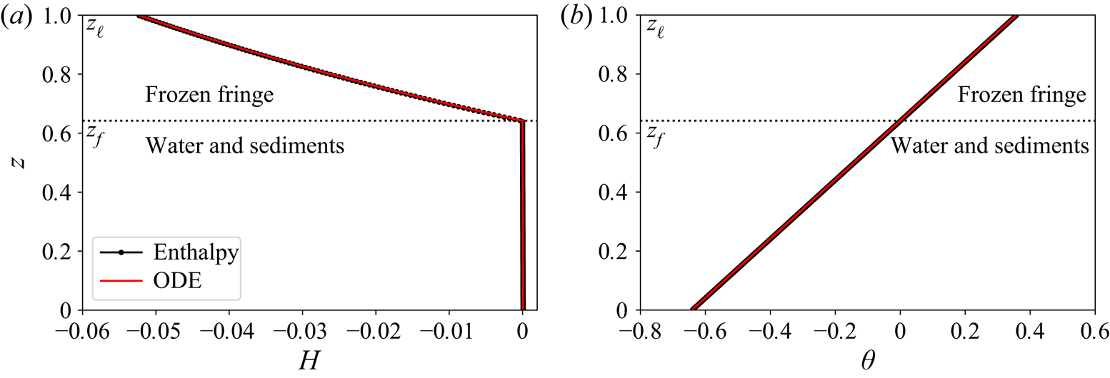
In figure 4, we show the dimensional fringe thickness  $h = [h](z_\ell - z_f)$ in metres as a function of the non-dimensional effective pressure $N/N_c$ for balanced ( $V=0$, figure 4a) and temperate melting ( $V = -q/(\rho _i \mathscr {L} [V])$, figure 4b) thermodynamics using five different solution methods. The first two techniques are what we just described: ‘ODE’ is the solution to (3.8) subject to (2.82) and ‘enthalpy’ is the conserved finite-volume method for solving (2.74). In the thermodynamically balanced case, (2.82) can be integrated exactly and the fringe thickness can be found with a root-finding algorithm, which we name ‘root’ in figure 4. The last two methods ‘uega’ and ‘shooting’ are from Rempel (Reference Rempel2008) and are run here using the parameters in table 1. In the uniform external gradient approximation (uega) method Rempel (Reference Rempel2008) maps the fringe with imposed external heat fluxes to a Stefan problem domain whereas the ‘shooting’ method searches for a consistent temperature at the base of the lowest ice lens. As expected, all five of these solution methods give the same result. The fringe thicknesses are much lower in the temperate melting case because the liquid pressure distribution in the fringe needed to expel meltwater supports a larger portion of the overburden and the fringe melts as the ice infiltrates into the sediments.
Compilation of benchmark solutions for dimensional fringe thickness  $h$ for two non-dimensional heave rates (a) $V=0$ and (b) $V=-q/(\rho _i \mathscr {L} [V]) = -1.1$. The ‘uega’ and ‘shooting’ are solution methods from Rempel (Reference Rempel2008). The ‘enthalpy’ solution is from the finite-volume method, ‘ODE’ is the steady-state ODE solution and ‘root’ is the semi-analytical root-finding method. All methods give the same result.

3.2. Ice lens initiation
In the calculation of the steady-state fringe thicknesses, we focused on melting ( $V<0$) and balanced ( $V=0$) thermodynamics. Although steady states do exist for relatively small freezing rates and relatively small effective pressures (Meyer et al. Reference Meyer, Downey and Rempel2018), transient behaviour such as ice lens initiation can occur when there is net freezing ( $V>0$). In figure 5, we show the local effective pressure $N_{loc}$ as a function of depth $z$ for melting (figure 5a) and freezing (figure 5b). Here the top of the domain is the lowest ice lens $z_\ell = 20$ and $N_{loc}$ is evaluated in the fringe region above $z_f \approx 18$ (a) and $z_f \approx 6$ (b). In the steady melting case, $N_{loc}$ monotonically increases from the ice lens to the effective pressure at the bottom of the fringe $N$. The low pressure at the base of the ice lens draws in water as the ice lens infiltrates into the sediments through regelation (Gilpin Reference Gilpin1980; Fowler & Krantz Reference Fowler and Krantz1994; Rempel & Meyer Reference Rempel and Meyer2019). In the transient freezing case, water is drawn into the fringe and freezes onto the base of the lowest ice lens. The ice saturation increases, which lowers the permeability and requires a larger hydrodynamic pressure gradient to continue freezing. The fringe thickens until, at some point in time, the local effective pressure reaches zero, i.e.
 \begin{equation} N_{loc}(z_n)=0, \end{equation}
and a new ice lens forms at  $z_n$.
Local effective pressure  $N_{loc}(z)$ with height $z$ scaled with the effective pressure $N$ at the base of the fringe for: (a) a melting steady state ( $V=-0.01$ and $N=2.9$) where $N_{loc}>0$ throughout the fringe and (b) a transient freezing simulation ( $V=0.20$ and $N=2.9$) where the local effective pressure goes to zero $N_{loc}(z_n)=0$, at point in the fringe $z_n$, initiating a new ice lens.
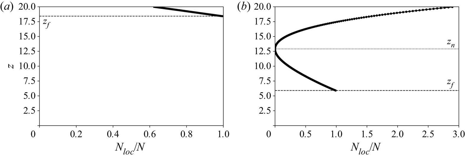
We determine the time when a new ice lens forms using the ‘events’ functionality built into  $\mathtt {solve\_ivp}$, which flags the location and time of the new ice lens as an event and stops the integration. We then shift our domain up so that the new ice lens is at the top and pad the bottom of the domain with water-saturated sediments following the same incoming heat flux. Then, we restart the integration until the next ice lens forms. Written inside a loop, we generate sequences of ice lenses with an interlens time $t_\ell$.
Using the constant heave rate  $V$ and interlens time $t_\ell$, we can reconstruct the porosity structure a posteriori. We treat the porosity as a constant $\phi$ in the fringe and water-saturated sediment. In the ice lenses, the porosity is also constant with $\phi =1$. In one vertical dimension, mass conservation for sediments from (2.1) is
 \begin{equation} \frac{\partial{\left( 1-\phi\right)}}{\partial{t}} + \frac{\partial{\left[V_s \left( 1-\phi\right)\right]}}{\partial{z}} = 0, \end{equation}
for a constant sediment density  $\rho _s$. If we say that the sediment advection $V_s$ is given by the heave according to
 \begin{equation} V_s = \begin{cases} 0, & \mbox{below the lowest lens,} \\ V, & \mbox{above the lowest lens,} \end{cases} \end{equation}
we find that
 \begin{equation} \frac{\partial{\phi}}{\partial{t}} + V \frac{\partial{\phi}}{\partial{z}} = 0, \end{equation}
above  $z_f$ because $V$ is constant in this region. This model assures that the ice lenses and interstitial fringe advect vertically as one unit of rigid ice (O'Neill & Miller Reference O'Neill and Miller1985). Importantly, this treatment assumes that there is no volume expansion upon freezing and the water freezes in place, treating the ice and water densities as equal. This approximation is valid to leading order in the scaled and simplified model we describe in § 2.7.2. We solve (3.12) equation analytically using the travelling-wave form, i.e.
 \begin{equation} \phi = f\left( z - V t\right), \end{equation}
which we apply at the initiation of each new ice lens, where we have that  $\phi = 1$ at $z=z_n$. The ice lens then grows at the rate $V$, lifting the overlying material following (3.12). In figure 6, we show the evolution of the porosity $\phi$ with time as three new ice lenses sequentially nucleate and grow. With these parameters, the lenses form periodically with equal spacing and interlens times.
Porosity structure of a freezing sediment pack. (a) Initial porosity profile with  $z_\ell =25$. The region above $z_\ell$ is the lowest ice lens and the region below is fringe as well as water-saturated sediments. (b) A posteriori travelling-wave solutions for porosity after initiation and growth of three periodic ice lenses. The non-dimensional parameters $V=0.5$ and $N=1.5$ and the non-dimensional interlens time is $t_{\ell }=9.6$.

3.3. Ice lens spacing
With a constant heave rate  $V$, the interlens time $t_{\ell }$ allows us to compute the ice lens spacing $\ell$ as
 \begin{equation} \ell = V t_{\ell}. \end{equation}
For a set value of the effective pressure  $N$, we find that the ice lens spacing $\ell$ decreases with an increasing heave rate $V$ (cf. figure 7). To capture the general trend of lens spacing with heave rate, we can scale the boundary condition at $z_{\ell }$ given in (2.78), which we repeat here
 \begin{equation} K\frac{\partial{\theta}}{\partial{z}} + {\textit{Pe}}\,VH = 1,\end{equation}
i.e. the Stefan condition at the interface. We take the temperature gradient to scale with the ice lens temperature  $\theta _{\ell }$ divided by the ice lens spacing $\ell$, take the thermal conductivity to scale as unity and set the ice saturation $S$ using the lens temperature $\theta _{\ell }$, with enthalpy in the fringe given by $H=-\phi S$. We find that
 \begin{equation} \ell\sim \frac{\theta_{\ell}}{1+{\textit{Pe}}\,V\phi S}.\end{equation}
For each simulation, we tabulate the ice lens spacing  $\ell$, the heave rate $V$ and the lens temperature $\theta _{\ell }$. We compare the simulation results and the (3.16) scaling in figure 7. At moderate $V$, (3.16) shows that there is a regime where the ice lens spacing is largely independent of the heaving rate and predominantly a function of the lens temperature (cf. Rempel et al. Reference Rempel, Wettlaufer and Worster2004; Rempel Reference Rempel2007). In this regime, the ice lens temperature becomes colder in pace with the increasing freezing rate, leading to a balance. For large $V$, (3.16) implies a scaling where $\ell \sim 1/V$. The rapid freezing rate does not allow the temperature at the lens to decrease concomitantly, and $\theta _{\ell }$ asymptotes to a constant value, leading to more closely spaced ice lenses. In figure 7(a), the blue line for (3.16) includes no fitting constants, whereas the black line for the $\ell \sim 1/V$ is proportional to a fitted prefactor for illustration. The vertical dashed line shows the heave rate onset of periodic lenses for this effective pressure. Heave rates below the dashed line support a steady fringe without producing periodic lenses, i.e. the interlens time $t_{\ell }$ is infinite. For heave rates slightly larger than the dashed line, the interlens time $t_{\ell }$ approaches infinity, leading to the uptick in lens spacing near the critical value.
Ice lens spacing  $\ell$ as a function of heave rate $V$. (a) Non-dimensional simulation results (green dots) compared with a $1/V$ (black line) and Stefan condition scalings (blue line) with $N=1.103$ and the default parameters from table 1. Dashed black vertical line shows the onset of period lenses. (b) Comparison between simulation results (black dots) and Wang et al. (Reference Wang, Wang, Ma, Wen, Chen and Xu2018) laboratory experiments (blue dots). Here we use parameters following the experiments, i.e. $N/N_c = 1.001$, $\alpha = 4$, $\phi =0.33$, $r_p = 60\times 10^{-6}$ m, $\rho _s = 2700\ {\rm kg}\ {\rm m}^{-3}$ and default otherwise. The model includes enthalpy evolution (2.74) with heave rate (2.82) subject to boundary conditions (2.78) and (2.79) as well as the ice lens nucleation condition (3.9).
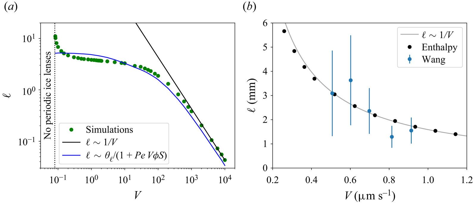
We compare our simulations for ice lens spacing to laboratory observations from Wang et al. (Reference Wang, Wang, Ma, Wen, Chen and Xu2018), as shown in figure 7(b). We select these experiments because of the range of heave rates and clear images. We digitised the spacing between lenses from their figure 5 at three points across the sample and show the mean as well as standard deviation as error bars. We computed the average heave rate  $\bar {V}_{Wang}$ for the experiment as
 \begin{equation} \bar{V}_{Wang} = \frac{K_i}{\rho_i \mathscr{L}} \frac{\Delta T}{h_0}, \end{equation}
from the temperature difference  $\Delta T$ and initial sample height $h_0$ given in their table 2. There are inherent errors in this tabulation of ice lens spacing and the approximation of the heave rate, but the general trend and model agreement are encouraging.
3.4. Regime diagram and subglacial observations
The two primary control parameters for the geophysical system are the heave rate  $V$ and the effective pressure $N$. So far we have shown steady states for balanced ( $V=0$) and melting ( $V<0$) conditions as well as ice lens initiation for freezing conditions ( $V>0$). In figure 8, we show a regime diagram for the system behaviour as a function of $V$ and $N$. Each point on the figure is a simulation and the colour denotes the grouping. For $N< N_c$, no fringe forms and the lens either melts or grows, depending on the sign of $V$. When $N>N_c$, ice infiltrates into the sediment forming a fringe. In melting or balanced cases where $V\le 0$, a steady-state fringe thickness emerges (e.g. figures 3 and 4). For positive heave rates $V>0$, steady states for relatively small effective pressures give way to periodic lenses as the heave rate increases. In the Appendix, we calculate the maximum steady fringe by considering the largest load that can be supported by a steady fringe. Just below this boundary between the steady and periodic regimes, there is a zone of hysteresis, where depending on the initial conditions the system either relaxes to a steady state or periodically generates new ice lenses, consistent with the Rempel et al. (Reference Rempel, Wettlaufer and Worster2004) regime diagram. Here we find that large freezing rates result in closely spaced ice lenses (cf.figure 7). Although we observe some small variability in the interlens times, we do not see anything reminiscent of the chaotic regime found by Anderson & Worster (Reference Anderson and Worster2014).
Regime diagram showing the system behaviour as a function of the heave rate  $V$ and effective pressure $N$. The maximum steady fringe thickness is shown as a solid black line and the theory is described in the Appendix.

Rempel et al. (Reference Rempel, Wettlaufer and Worster2004) constructed their regime diagram with constant heat flux experiments in mind, whereas the regime diagram of Rempel (Reference Rempel2007) was designed for the step freezing sub-aerial case. In contrast, here we focus on the geophysical applications, e.g. subglacial behaviour, permafrost regions and frost-heaving soils. A key difference between our figure 8 and the previously published regime diagrams are the variables plotted on both axes. While we define  $N$ as the difference between the ice and water pressures at min( $z_f, z_l$), the unscaled $p_0$ in figure 8 of Rempel et al. (Reference Rempel, Wettlaufer and Worster2004) is the gauge pressure of the ice itself, with the water pressure defined as hydrostatic at some location $z_h$ that is treated as 0 in all of their calculated results. Partly as a result, the boundary at $N_c$ between lens no fringe and (i) steady lens with fringe, (ii) hysteresis or (iii) periodic lensing that we find is not a reproduction of the result from Rempel et al. (Reference Rempel, Wettlaufer and Worster2004). Figure 8 of Rempel et al. (Reference Rempel, Wettlaufer and Worster2004) also has a different $y$-axis. The scaled $v$ in Rempel et al. (Reference Rempel, Wettlaufer and Worster2004) is the constant pulling rate or imposed rate of advance of isotherms. In our new work it is the heave rate, or rate of advance of the lens boundary. Because of this difference, in the treatment of Rempel et al. (Reference Rempel, Wettlaufer and Worster2004) there is the potential for sufficiently rapid freezing that no lenses can nucleate, leading to a region of their regime diagram that collapses onto the $x$-axis in our new regime diagram. The regime diagram of Rempel et al. (Reference Rempel, Wettlaufer and Worster2004) focused on experimental controls (pulling speed and applied load) with water pressure set at a remote warm location rather than the furthest extent of pore ice. The regime diagram we develop here focuses on key system observables, i.e. heave rate and effective pressure. Rempel (Reference Rempel2007) shows regime diagrams for different soils in figures 7 and 8, but these are plotted with axes of $P_0$ and undercooling, which is related but distinct from our results.
Based on figure 8, if we have estimates for  $V$ and $N$ in a geophysical context such as below a glacier, we can predict the system behaviour such as whether ice lenses will form. For example, Rada & Schoof (Reference Rada and Schoof2018) measure the effective pressure $N = 87$ kPa in a subglacial conduit. With $N_c = 68$ kPa, the ratio is $N/N_c = 1.3$ and if we take balanced thermodynamics $V=0$, then the resulting fringe thickness in the sediments adjacent to the conduit will be about 40 cm (0.23 $[z]$). Results for similar parameters are shown in figure 3 and the same value could be read off of figure 4(a). For melting below temperate ice at $V=-1.1$ corresponding to $7.9\ {\rm mm}\ {\rm year}^{-1}$, the predicted fringe is about 20 cm thick (0.11 $[z]$), as shown in figure 4(b) and closer to observations from Rada & Schoof (Reference Rada and Schoof2018).
4. Conclusions
In this paper, we have derived the thermodynamical and fluid mechanical equations governing frost heave in a geophysical context. We have systematically reduced the equations using the fact that ice and water have similar densities (i.e. small  $\delta$) as well as the large Stefan number ${\textit{St}}$. We have solved the reduced set of equations using an enthalpy method where the interstitial ice saturation acts like a liquidus condition in the frozen fringe and conservation of enthalpy allows us to determine the fringe interface implicitly. For melting and balanced thermodynamics, we have compared our enthalpy method to a steady state obtained by solving an ordinary differential equation for temperature and found excellent agreement. In freezing cases, we have found that the local effective pressure can go to zero within the fringe and nucleate a new ice lens. We accommodate this process in our enthalpy model using an ‘events’ function that stops the integration when a new ice lens forms and restarts the integration with a domain shifted below the new ice lens. Based on our solutions for the time between lenses, we have reconstructed the porosity profile showing the sequence of ice lenses. We have found that the spacing of ice lenses follows a scaling set by the Stefan condition and that the simulation results agreed with experimental data. Finally, we have compiled a regime diagram of our simulation results, showing the onset of periodic lensing and behaviour including hysteresis. Our results advance the understanding of frozen sediments in subaerial and subglacial environments through providing a systematic scaling of the full model, a novel numerical implementation and a new scaling for ice lens spacing which we have compared directly with laboratory experiments. Our regime diagram shows similar features to previous work, but is tailored to the geophysical environment. Our results inform the interpretation of geophysical systems and are a foundation for future investigations into the role of compaction as well as further comparisons with laboratory experiments.
Acknowledgements
We thank L. Arenson, A. Fowler, I. Hewitt and L. Zoet for insightful conversations. A.W.R. and C.S. are grateful to have participated in the 2006 Geophysical Fluid Dynamics summer school at the Woods Hole Oceanographic Institution, where part of this collaboration began.
Funding
We acknowledge support from NSF-2012958 (CRM and AWR) and NSF-1603907 (AWR) as well as ERDC/CRREL-W913E519C0008 (CRM) and NASA-80NSSC21M0329 (CRM).
Declaration of interests
The authors report no conflict of interest.
Appendix. Steady heave near thermal balance
For an effective pressure  $N$ greater than the infiltration threshold $N_c$, a steady fringe will form for melting ( $V<0$), balanced ( $V=0$) and weakly freezing ( $0< V< V_{max}(N)$) thermodynamics, where $V_{max}$ depends on the effective pressure $N$ (namely, figures 4 and 8). Alternatively, the maximum freezing heave rate can be thought of in the reverse: for a given heave rate ( $V>0$), there is a maximum effective pressure $N_{max}(V)$, which is the largest load that can be supported by a steady fringe. For larger effective pressures, periodic lenses form. Here we will show how to calculate $V_{max}(N)$ and $N_{max}(V)$.
We start by rearranging (2.82) for  $N$, which is
 \begin{align} N =1 + {\textit{G}}\left(\nu-1\right) (1-\phi) \left(z_{\ell}- z_f\right) + \int_{z_f}^{z_{\ell}}\left( 1 - \phi S\right)\frac{\partial{\theta}}{\partial{z'}}\,{\rm d}z' - V\int_{z_f}^{z_{\ell}}\frac{(1-\phi S)^2}{k}\,{\rm d}z'. \end{align}
To find the maximum effective pressure, we treat  $z_f$ as fixed and set the derivative of $N$ with respect to $z_\ell$ equal to zero, i.e.
 \begin{equation} \frac{\partial{N}}{\partial{z_\ell}} ={\textit{G}}\left(\nu-1\right) (1-\phi) + \left.\left( 1 - \phi S\right)\frac{\partial{\theta}}{\partial{z}}\right|_{z_\ell} - V\left.\frac{(1-\phi S)^2}{k}\right|_{z_\ell} = 0. \end{equation}
Treating the thermal conductivity variation as negligible, we insert the heat flux from (3.8) to find
 \begin{equation} {\textit{G}}\left(\nu-1\right) (1-\phi) + \left[ 1 - \phi S(\theta_\ell^*)\right] \left[1 + {\textit{Pe}}\,V\phi S(\theta_\ell^*)\right] - V\frac{\left[1-\phi S(\theta_\ell^*)\right]^2}{k(\theta_\ell^*)} = 0, \end{equation}
which can be solved using a root-finding algorithm for the lens temperature  $\theta _\ell ^*(V)$, i.e. the lowest lens temperature that can be supported for a given heave rate $V$. We now change the integration variable from $z$ to $\theta$ in the force balance equation (A1) using (3.8) and use the minimum lens temperature $\theta _{\ell }^*$ in the limits of integration, i.e.
 \begin{align} N &=1 +
\int_{0}^{\theta_\ell^*(V)}{\frac{{\textit{G}}\left(\nu-1\right)
(1-\phi)}{1 + {\textit{Pe}}\,V\phi S(\theta)}\,{\rm d}\theta} +
\int_{0}^{\theta_\ell^*(V)}\left[ 1 - \phi
S(\theta)\right]{\rm d}\theta \nonumber\\ &\quad -
V\int_{0}^{\theta_\ell^*(V)}\frac{[1-\phi
S(\theta)]^2}{k(\theta) \left[1 + {\textit{Pe}}\,V\phi
S(\theta)\right]}\,{\rm d}\theta.
\end{align}
\begin{align} N &=1 +
\int_{0}^{\theta_\ell^*(V)}{\frac{{\textit{G}}\left(\nu-1\right)
(1-\phi)}{1 + {\textit{Pe}}\,V\phi S(\theta)}\,{\rm d}\theta} +
\int_{0}^{\theta_\ell^*(V)}\left[ 1 - \phi
S(\theta)\right]{\rm d}\theta \nonumber\\ &\quad -
V\int_{0}^{\theta_\ell^*(V)}\frac{[1-\phi
S(\theta)]^2}{k(\theta) \left[1 + {\textit{Pe}}\,V\phi
S(\theta)\right]}\,{\rm d}\theta.
\end{align}
For a given value of  $N$, we use another root-finding algorithm to find the heave rate $V$ that satisfies (A4), which is the maximum heave rate with a steady fringe. Repeated application of this root-finding algorithm results in the black curve $V_{max}(N)$ shown on figure 8 and partitions the periodic lens regime from the hysteresis/steady lens regime.


 Open access