


1 Introduction
Transitional flow past a blade in a compressor passage has been thoroughly investigated owing to its rich dynamics associated with pressure gradients, free-stream noise, leading-edge effects and surface curvature (Gostelow, Blunden & Walker Reference Gostelow, Blunden and Walker1994; Spalart & Strelets Reference Spalart and Strelets2000). Both orderly and bypass transition scenarios have been observed to occur on various sections of the blade (Zaki et al. Reference Zaki, Wissink, Rodi and Durbin2010). In the present work, the linear perturbation growth that triggers transition is studied.
1.1 Transition induced by instability waves
Breakdown to turbulence triggered by instability waves, e.g. Tollmien–Schlichting (TS) waves, is commonly termed orderly transition in boundary-layer flows. In this scenario, spanwise periodic $\unicode[STIX]{x1D6EC}$
structures have been observed to develop on top of TS waves (Klebanoff, Tidstorm & Sargent Reference Klebanoff, Tidstorm and Sargent1962). These structures can be further stretched by the mean shear to create hairpin vortices before breaking down to turbulence. In terms of perturbation growth, the
$\unicode[STIX]{x1D6EC}$
structures have been observed to develop on top of TS waves (Klebanoff, Tidstorm & Sargent Reference Klebanoff, Tidstorm and Sargent1962). These structures can be further stretched by the mean shear to create hairpin vortices before breaking down to turbulence. In terms of perturbation growth, the $\unicode[STIX]{x1D6EC}$
structures are associated with three-dimensional (3-D) secondary instabilities of two-dimensional (2-D) TS waves. In the present work,
$\unicode[STIX]{x1D6EC}$
structures are associated with three-dimensional (3-D) secondary instabilities of two-dimensional (2-D) TS waves. In the present work, $\unicode[STIX]{x1D6EC}$
structures are also observed, but are created in the nonlinear evolution of 3-D optimal initial perturbations that are firstly amplified by the linear Orr mechanism (Orr Reference Orr1907).
$\unicode[STIX]{x1D6EC}$
structures are also observed, but are created in the nonlinear evolution of 3-D optimal initial perturbations that are firstly amplified by the linear Orr mechanism (Orr Reference Orr1907).
In direct numerical simulations (DNS) of a NACA 65 blade geometry, adverse pressure gradient and separation are observed on most of the blade surface except the leading edge on the suction surface and trailing edge on the pressure surface (Zaki et al. Reference Zaki, Wissink, Rodi and Durbin2010). When the pressure gradient is adverse, the boundary-layer profile becomes inflectional and therefore is prone to inviscid instabilities. If the adverse pressure gradient is sufficiently strong, the boundary layer separates and generates detached rolls. These rolls are subject to 3-D instabilities, which induce transition when the unstable modes saturate. In this process, the strong reverse flow in braid regions, which advects perturbations upstream and therefore keeps the rolls perturbed, is critical for the instability to sustain itself (Jones, Sandberg & Sandham Reference Jones, Sandberg and Sandham2008; Zaki et al. Reference Zaki, Wissink, Rodi and Durbin2010). It has been also reported that small-scale perturbations in the wake are responsible for triggering transition inside the Kelvin–Helmholtz (K–H) rolls (Wissink & Rodi Reference Wissink and Rodi2006). Rocco et al. (Reference Rocco, Zaki, Mao, Blackburn and Sherwin2015) have applied a Floquet stability analysis to the phase-averaged unsteady base flow to study the flow stability downstream of the separation bubble.
1.2 Bypass transition
Bypass transition refers to scenarios where breakdown to turbulence does not strictly follow the orderly route. High- and low-speed velocity streaks are typically observed. The flow in the streaks is dominated by the streamwise velocity component. These streaks have spanwise wavenumber higher than the $\unicode[STIX]{x1D6EC}$
structures introduced above and are elongated in the streamwise direction. The transition to turbulence is initiated by the distortion or secondary instabilities, of the streaks around the top of the boundary layer, activated by high-frequency noise in the free stream (Jacobs & Durbin Reference Jacobs and Durbin2001).
$\unicode[STIX]{x1D6EC}$
structures introduced above and are elongated in the streamwise direction. The transition to turbulence is initiated by the distortion or secondary instabilities, of the streaks around the top of the boundary layer, activated by high-frequency noise in the free stream (Jacobs & Durbin Reference Jacobs and Durbin2001).
The streaks can be generated by streamwise vortices, which tilt the mean shear via a linear ‘lift-up’ mechanism (Phillips Reference Phillips1969). In linear theory, low- and high-speed streaks have identical spanwise velocity profiles, and they alternate periodically in the span. In DNS, however, the spanwise velocity profiles of high- and low-speed streaks differ. In the present work, a nonlinear mechanism is proposed to explain their form, or specifically how the low-speed streaks are lifted above the high-speed ones. Streamwise vortices have been found to be optimal initial perturbations in boundary-layer flow without a leading edge (Andersson, Berggren & Henningson Reference Andersson, Berggren and Henningson1999; Monokrousos et al. Reference Monokrousos, Åkervik, Brandt and Henningson2010). In a swept-wing boundary-layer flow with a leading edge, the optimal free-stream perturbation yielding maximum receptivity amplitude at a downstream location was found to take the form of a streak (Tempelmann et al. Reference Tempelmann, Schrader, Hani, Brandt and Henningson2012). In the present work, a free-stream optimal initial perturbation in the form of streamwise vortices upstream of the leading edge is obtained for the first time.
Broadband free-stream vortical forcing causes the amplification of boundary-layer streaks and induces bypass transition in DNS (Jacobs & Durbin Reference Jacobs and Durbin2001). Zaki & Durbin (Reference Zaki and Durbin2005) were able to reproduce the same features using only two free-stream vortical perturbations. When both free-stream forcing and TS waves are present, breakdown to turbulence features $\unicode[STIX]{x1D6EC}$
structures (similar to the secondary instability of TS waves), whose spanwise wavenumber is related with the streaks (Liu, Zaki & Durbin Reference Liu, Zaki and Durbin2008).
$\unicode[STIX]{x1D6EC}$
structures (similar to the secondary instability of TS waves), whose spanwise wavenumber is related with the streaks (Liu, Zaki & Durbin Reference Liu, Zaki and Durbin2008).
1.3 Secondary instabilities of streaks
When the magnitude of the streaks is sufficiently large, streamwise travelling waves are excited and the streaks start to lose stability and ultimately break down to turbulence. Brandt et al. (Reference Brandt, Cossu, Chomaz, Huerre and Henningson2003) found that the instability of optimal streaks is convective and that the streaks behave as amplifiers of external noise. The secondary instabilities and the associated modes can be calculated through linear Floquet analyses of the streak base flow extracted from DNS or experiential results (Elofsson, Kawakami & Alfredsson Reference Elofsson, Kawakami and Alfredsson1999; Ricco, Luo & Wu Reference Ricco, Luo and Wu2011).
Two types of secondary instabilities of streaks, inner mode and outer mode, have been obtained by using either idealized streaks or real streaks extracted from DNS as the base flow (Vaughan & Zaki Reference Vaughan and Zaki2011; Hack & Zaki Reference Hack and Zaki2014). The inner modes, which occur around the local overlap between high- and low-speed streaks, are symmetric and are also termed as varicose modes. The outer modes, which occur around low-speed streaks that are lifted towards the edge of the boundary layer, are anti-symmetric and are also termed as sinuous modes. The critical streak amplitudes for the streaks to lose stability to inner and outer modes are 26 % and 37 %, respectively (Andersson et al. Reference Andersson, Brandt, Bottaro and Henningson2001). Blasius boundary layers favour the amplification of outer instabilities, while an adverse pressure gradient promotes breakdown to turbulence via the inner mode, as observed in a statistical study by Hack & Zaki (Reference Hack and Zaki2014). Earlier results by Swearingen & Blackwelder (Reference Swearingen and Blackwelder1987) in the context of Görtler vortices, and by Ehrenstein, Marquillie & Laval (Reference Ehrenstein, Marquillie and Laval2011) in channel flow with a lower curved wall can be ascribed to the inner and outer classes.
1.4 Motivations of the present work
The main objective of the present work is to examine the linear mechanisms behind the laminar–turbulent transition on various regions of the compressor blade, with a focus on bypass transition triggered by noise upstream of the leading edge. To be aligned with previous studies, we adopt a NACA 65 blade at $44^{\circ }$
incidence and chord Reynolds number
$44^{\circ }$
incidence and chord Reynolds number $138\,500$
(Hilgenfeld & Pfitzner Reference Hilgenfeld and Pfitzner2004; Zaki et al.
Reference Zaki, Durbin, Wissink and Rodi2006, Reference Zaki, Wissink, Rodi and Durbin2010; Rocco et al.
Reference Rocco, Zaki, Mao, Blackburn and Sherwin2015). The phase-averaged base flow around the shedding vortices on the suction side has been found to be globally most unstable in Floquet analyses (Rocco et al.
Reference Rocco, Zaki, Mao, Blackburn and Sherwin2015). In the present work, a transient growth analysis is adopted, and the base flow is the time-dependent solution of the NS equations without phase averaging. Furthermore, a weight factor is applied to filter perturbation growth in the globally most unstable region and subsequently enable the examination of perturbation development in any regions of interest (Schmidt et al.
Reference Schmidt, Hosseini, Rist, Hanifi and Henningson2015; Theobald et al.
Reference Theobald, Mao, Jaworski and Berson2015). Through this approach, we can spatially localize the analysis, and the optimal perturbation located upstream of the leading edge as well as the induced bypass transition is highlighted. During the development of this optimal perturbation, streamwise velocity streaks are generated via a linear lift-up mechanism. These streaks are shifted to an unstable layout through a nonlinear lift-up mechanism before breaking up into turbulence.
$138\,500$
(Hilgenfeld & Pfitzner Reference Hilgenfeld and Pfitzner2004; Zaki et al.
Reference Zaki, Durbin, Wissink and Rodi2006, Reference Zaki, Wissink, Rodi and Durbin2010; Rocco et al.
Reference Rocco, Zaki, Mao, Blackburn and Sherwin2015). The phase-averaged base flow around the shedding vortices on the suction side has been found to be globally most unstable in Floquet analyses (Rocco et al.
Reference Rocco, Zaki, Mao, Blackburn and Sherwin2015). In the present work, a transient growth analysis is adopted, and the base flow is the time-dependent solution of the NS equations without phase averaging. Furthermore, a weight factor is applied to filter perturbation growth in the globally most unstable region and subsequently enable the examination of perturbation development in any regions of interest (Schmidt et al.
Reference Schmidt, Hosseini, Rist, Hanifi and Henningson2015; Theobald et al.
Reference Theobald, Mao, Jaworski and Berson2015). Through this approach, we can spatially localize the analysis, and the optimal perturbation located upstream of the leading edge as well as the induced bypass transition is highlighted. During the development of this optimal perturbation, streamwise velocity streaks are generated via a linear lift-up mechanism. These streaks are shifted to an unstable layout through a nonlinear lift-up mechanism before breaking up into turbulence.
The methodology of spatially weighted transient growth is introduced in § 2; the numerical method is discussed in § 3; the linear and nonlinear perturbation growth in three typical regions are presented in §§ 4–6. Finally conclusions are drawn in § 7.
2 Optimal transient growth methodology
Assuming the fluid is Newtonian and the flow is incompressible, the non-dimensionalized Navier–Stokes (NS) equations are:
 $$\begin{eqnarray}\unicode[STIX]{x2202}_{t}\boldsymbol{u}=-\boldsymbol{u}\boldsymbol{\cdot }\unicode[STIX]{x1D735}\boldsymbol{u}-\unicode[STIX]{x1D735}p+Re^{-1}\unicode[STIX]{x1D6FB}^{2}\boldsymbol{u},\quad \unicode[STIX]{x1D735}\boldsymbol{\cdot }\boldsymbol{u}=0,\end{eqnarray}$$
where $t$
denotes the time coordinate;
$t$
denotes the time coordinate; $Re$
is the Reynolds number based on the inflow velocity and the axial blade chord length (see figure 1);
$Re$
is the Reynolds number based on the inflow velocity and the axial blade chord length (see figure 1); $\boldsymbol{u}$
is the velocity vector field and
$\boldsymbol{u}$
is the velocity vector field and $p$
denotes pressure, all considered in a spatial domain
$p$
denotes pressure, all considered in a spatial domain $\unicode[STIX]{x1D6FA}$
. Decomposing the flow field into the sum of a base flow and a perturbation,
$\unicode[STIX]{x1D6FA}$
. Decomposing the flow field into the sum of a base flow and a perturbation, $\boldsymbol{u}=\boldsymbol{U}+\boldsymbol{u}^{\prime }$
,
$\boldsymbol{u}=\boldsymbol{U}+\boldsymbol{u}^{\prime }$
, $p=P+p^{\prime }$
, inserting into (2.1), and retaining only terms linear in the perturbation, one obtains the linearized NS equations
$p=P+p^{\prime }$
, inserting into (2.1), and retaining only terms linear in the perturbation, one obtains the linearized NS equations
 $$\begin{eqnarray}\unicode[STIX]{x2202}_{t}\boldsymbol{u}^{\prime }=-\boldsymbol{U}\boldsymbol{\cdot }\unicode[STIX]{x1D735}\boldsymbol{u}^{\prime }-\boldsymbol{u}^{\prime }\boldsymbol{\cdot }\unicode[STIX]{x1D735}\boldsymbol{U}-\unicode[STIX]{x1D735}p^{\prime }+Re^{-1}\unicode[STIX]{x1D6FB}^{2}\boldsymbol{u}^{\prime },\quad \unicode[STIX]{x1D735}\boldsymbol{\cdot }\boldsymbol{u}^{\prime }=0.\end{eqnarray}$$
If the base flow is homogeneous in one direction, e.g. the spanwise direction, the perturbation can be further decomposed, such that $\boldsymbol{u}^{\prime }=\sum _{\unicode[STIX]{x1D6FD}=0}^{\infty }\hat{\boldsymbol{u}}_{\unicode[STIX]{x1D6FD}}\exp (\text{i}\unicode[STIX]{x1D6FD}z)+\text{c.c.}$
, where
$\boldsymbol{u}^{\prime }=\sum _{\unicode[STIX]{x1D6FD}=0}^{\infty }\hat{\boldsymbol{u}}_{\unicode[STIX]{x1D6FD}}\exp (\text{i}\unicode[STIX]{x1D6FD}z)+\text{c.c.}$
, where $\unicode[STIX]{x1D6FD}$
is the spanwise wavenumber. Since the governing equations (2.2) are linearized, Fourier modes with different
$\unicode[STIX]{x1D6FD}$
is the spanwise wavenumber. Since the governing equations (2.2) are linearized, Fourier modes with different $\unicode[STIX]{x1D6FD}$
are decoupled and can be studied separately. In the following, the term perturbation refers to the Fourier mode and the subscript
$\unicode[STIX]{x1D6FD}$
are decoupled and can be studied separately. In the following, the term perturbation refers to the Fourier mode and the subscript $\unicode[STIX]{x1D6FD}$
will be omitted.
$\unicode[STIX]{x1D6FD}$
will be omitted.
To evaluate the growth of disturbances over the entire or a part of the domain, we define the optimal transient growth of perturbations over time $\unicode[STIX]{x1D70F}$
as
$\unicode[STIX]{x1D70F}$
as
 $$\begin{eqnarray}G=\max _{\hat{\boldsymbol{u}}(0)}\frac{(F\hat{\boldsymbol{u}}(\unicode[STIX]{x1D70F}),F\hat{\boldsymbol{u}}(\unicode[STIX]{x1D70F}))}{(\hat{\boldsymbol{u}}(0),\hat{\boldsymbol{u}}(0))}=\max _{\hat{\boldsymbol{u}}(0)}\frac{(F{\mathcal{A}}\hat{\boldsymbol{u}}(0),F{\mathcal{A}}\hat{\boldsymbol{u}}(0))}{(\hat{\boldsymbol{u}}(0),\hat{\boldsymbol{u}}(0))},\end{eqnarray}$$
where $F$
is a scalar spatial window function which isolates the region of interest, with value 0 to 1; the inner product is defined as
$F$
is a scalar spatial window function which isolates the region of interest, with value 0 to 1; the inner product is defined as $(\boldsymbol{a},\boldsymbol{b})\equiv \int _{\unicode[STIX]{x1D6FA}}\boldsymbol{a}\boldsymbol{\cdot }\boldsymbol{b}\,\text{d}v$
;
$(\boldsymbol{a},\boldsymbol{b})\equiv \int _{\unicode[STIX]{x1D6FA}}\boldsymbol{a}\boldsymbol{\cdot }\boldsymbol{b}\,\text{d}v$
; ${\mathcal{A}}$
is an operator whose action is obtained by integrating the linearized NS equations;
${\mathcal{A}}$
is an operator whose action is obtained by integrating the linearized NS equations; $\unicode[STIX]{x1D70F}$
represents the time interval to calculate the optimal transient growth.
$\unicode[STIX]{x1D70F}$
represents the time interval to calculate the optimal transient growth.

Considering that the function $F$
satisfies
$F$
satisfies $(\boldsymbol{a},F\boldsymbol{b})=(F\boldsymbol{a},\boldsymbol{b})$
, equation (2.3) can be reformulated as
$(\boldsymbol{a},F\boldsymbol{b})=(F\boldsymbol{a},\boldsymbol{b})$
, equation (2.3) can be reformulated as
 $$\begin{eqnarray}G=\max _{\hat{\boldsymbol{u}}(0)}\frac{({\mathcal{A}}^{\ast }F^{2}{\mathcal{A}}\hat{\boldsymbol{u}}(0),\hat{\boldsymbol{u}}(0))}{(\hat{\boldsymbol{u}}(0),\hat{\boldsymbol{u}}(0))},\end{eqnarray}$$
where ${\mathcal{A}}^{\ast }$
is the adjoint operator of
${\mathcal{A}}^{\ast }$
is the adjoint operator of ${\mathcal{A}}$
satisfying
${\mathcal{A}}$
satisfying $(\boldsymbol{a},{\mathcal{A}}\boldsymbol{b})=({\mathcal{A}}^{\ast }\boldsymbol{a},\boldsymbol{b})$
. The action of
$(\boldsymbol{a},{\mathcal{A}}\boldsymbol{b})=({\mathcal{A}}^{\ast }\boldsymbol{a},\boldsymbol{b})$
. The action of ${\mathcal{A}}^{\ast }$
can be obtained by integrating the adjoint equation:
${\mathcal{A}}^{\ast }$
can be obtained by integrating the adjoint equation:
 $$\begin{eqnarray}-\unicode[STIX]{x2202}_{t}\boldsymbol{u}^{\ast }=\boldsymbol{U}\boldsymbol{\cdot }\unicode[STIX]{x1D735}\boldsymbol{u}^{\ast }-\boldsymbol{u}^{\ast }\boldsymbol{\cdot }(\unicode[STIX]{x1D735}\boldsymbol{U})^{\text{T}}-\unicode[STIX]{x1D735}p^{\ast }+Re^{-1}\unicode[STIX]{x1D6FB}^{2}\boldsymbol{u}^{\ast },\quad \text{with}~\unicode[STIX]{x1D735}\boldsymbol{\cdot }\boldsymbol{u}^{\ast }=0.\end{eqnarray}$$
From (2.4), the optimal growth $G$
and the corresponding optimal initial perturbation are the largest eigenvalue and the corresponding eigenvector of the operator
$G$
and the corresponding optimal initial perturbation are the largest eigenvalue and the corresponding eigenvector of the operator ${\mathcal{A}}^{\ast }(\unicode[STIX]{x1D70F})F^{2}{\mathcal{A}}(\unicode[STIX]{x1D70F})$
. Therefore the optimal energy growth (and the corresponding optimal initial perturbation) can be obtained by applying an Arnoldi method to a Krylov sequence, established by repeated action the joint operator
${\mathcal{A}}^{\ast }(\unicode[STIX]{x1D70F})F^{2}{\mathcal{A}}(\unicode[STIX]{x1D70F})$
. Therefore the optimal energy growth (and the corresponding optimal initial perturbation) can be obtained by applying an Arnoldi method to a Krylov sequence, established by repeated action the joint operator ${\mathcal{A}}^{\ast }(\unicode[STIX]{x1D70F})F^{2}{\mathcal{A}}(\unicode[STIX]{x1D70F})$
on a random initial perturbation (Barkley, Blackburn & Sherwin Reference Barkley, Blackburn and Sherwin2008).
${\mathcal{A}}^{\ast }(\unicode[STIX]{x1D70F})F^{2}{\mathcal{A}}(\unicode[STIX]{x1D70F})$
on a random initial perturbation (Barkley, Blackburn & Sherwin Reference Barkley, Blackburn and Sherwin2008).
The calculation can be performed according to the following steps.
-
(i) Initialize the perturbation velocity $\boldsymbol{u}^{\prime }(0)$
using 2-D white noise with a prescribed spanwise wavenumber.
$\boldsymbol{u}^{\prime }(0)$
using 2-D white noise with a prescribed spanwise wavenumber. -
(ii) Integrate the linearized NS equations (2.2) to obtained
${\mathcal{A}}\boldsymbol{u}^{\prime }(0)$
. -
(iii) Apply the weight function to the final velocity condition to obtain
$F^{2}{\mathcal{A}}\boldsymbol{u}^{\prime }(0)$
. -
(iv) Use the weighted velocity to initialize the adjoint velocity variables.
-
(v) Integrate the adjoint equation to calculate
${\mathcal{A}}^{\ast }F^{2}{\mathcal{A}}\boldsymbol{u}^{\prime }(0)$
. -
(vi) Apply an Arnoldi method to extract the leading eigenvalue and eigenvector of
${\mathcal{A}}^{\ast }F^{2}{\mathcal{A}}$
. If not converged, return to step (ii).


In this calculation, the weight function $F$
localizes the outcome of the initial perturbation. Similar localization techniques have been adopted to restrict the spatial extension of perturbation outcomes (Theobald et al.
Reference Theobald, Mao, Jaworski and Berson2015) or optimal initial perturbations (Schmidt et al.
Reference Schmidt, Hosseini, Rist, Hanifi and Henningson2015). The advantage of this approach is that boundary conditions of the region of interest are handled implicitly at the edges of the window and therefore one is free to choose the scope of the objective to be optimized. Note that when
$F$
localizes the outcome of the initial perturbation. Similar localization techniques have been adopted to restrict the spatial extension of perturbation outcomes (Theobald et al.
Reference Theobald, Mao, Jaworski and Berson2015) or optimal initial perturbations (Schmidt et al.
Reference Schmidt, Hosseini, Rist, Hanifi and Henningson2015). The advantage of this approach is that boundary conditions of the region of interest are handled implicitly at the edges of the window and therefore one is free to choose the scope of the objective to be optimized. Note that when $F$
is not constant across the domain, the initial condition of the adjoint operator, e.g.
$F$
is not constant across the domain, the initial condition of the adjoint operator, e.g. $F^{2}{\mathcal{A}}(\unicode[STIX]{x1D70F})\hat{\boldsymbol{u}}(0)$
, can become non-solenoidal. The results presented herein are not affected by this issue – a point addressed in appendix A. We note that the form of the optimal initial perturbation may not be observed directly in practical configurations. However, the downstream response highlights the preferred form of the perturbation field when the flow is exposed to random, inflow noise. Another noteworthy point is that the present approach evaluates the linearly optimal disturbance, while for large optimal perturbations a nonlinear optimization should be adopted (Pringle & Kerswell Reference Pringle and Kerswell2010).
$F^{2}{\mathcal{A}}(\unicode[STIX]{x1D70F})\hat{\boldsymbol{u}}(0)$
, can become non-solenoidal. The results presented herein are not affected by this issue – a point addressed in appendix A. We note that the form of the optimal initial perturbation may not be observed directly in practical configurations. However, the downstream response highlights the preferred form of the perturbation field when the flow is exposed to random, inflow noise. Another noteworthy point is that the present approach evaluates the linearly optimal disturbance, while for large optimal perturbations a nonlinear optimization should be adopted (Pringle & Kerswell Reference Pringle and Kerswell2010).
3 Discretization and convergence
Flow through a low-pressure compressor passage comprised of NACA 65 blades is examined, and the configuration is based on the experiments by Hilgenfeld & Pfitzner (Reference Hilgenfeld and Pfitzner2004). The governing equations are discretized via quadrilateral spectral elements with nodal tensor-product expansion bases in the $x{-}y$
plane, and Fourier decomposed in the spanwise
$x{-}y$
plane, and Fourier decomposed in the spanwise $z$
direction. A second-order backward-difference time-splitting scheme with equal-order interpolation of velocity and pressure is used for time integration (Karniadakis, Israeli & Orszag Reference Karniadakis, Israeli and Orszag1991). A side view of the computational domain is provided in figure 1, with 10 340 spectral elements in each
$z$
direction. A second-order backward-difference time-splitting scheme with equal-order interpolation of velocity and pressure is used for time integration (Karniadakis, Israeli & Orszag Reference Karniadakis, Israeli and Orszag1991). A side view of the computational domain is provided in figure 1, with 10 340 spectral elements in each $x{-}y$
plane. The domain is repeated in the
$x{-}y$
plane. The domain is repeated in the $y$
-direction for clarity. The grid resolution is determined based on the discretization and pressure distributions in Zaki et al. (Reference Zaki, Wissink, Rodi and Durbin2010). The number of Fourier modes calculated in the spanwise direction depends on the spanwise domain size and will be reported for each case in the following sections. We note that the outflow section is significantly elongated in order to accommodate the unsteady wake, which acts as an ‘amplifier’ to upstream disturbances.
$y$
-direction for clarity. The grid resolution is determined based on the discretization and pressure distributions in Zaki et al. (Reference Zaki, Wissink, Rodi and Durbin2010). The number of Fourier modes calculated in the spanwise direction depends on the spanwise domain size and will be reported for each case in the following sections. We note that the outflow section is significantly elongated in order to accommodate the unsteady wake, which acts as an ‘amplifier’ to upstream disturbances.
The boundary conditions are also denoted in figure 1. An incident free-stream velocity at $42^{\circ }$
is applied at the inflow boundary. A stress-free outflow velocity condition combined with a zero pressure condition is adopted for (2.1), while a zero Dirichlet velocity condition is used for (2.2) and (2.5) (Blackburn, Barkley & Sherwin Reference Blackburn, Barkley and Sherwin2008). Whenever the velocity condition is of the Dirichlet type, a high-order computed Neumann condition is applied for the pressure term (Karniadakis et al.
Reference Karniadakis, Israeli and Orszag1991). On the upper and lower boundaries, conditions are applied for both velocity and pressure. The Reynolds number based on the inflow velocity and the axial chord length is
$42^{\circ }$
is applied at the inflow boundary. A stress-free outflow velocity condition combined with a zero pressure condition is adopted for (2.1), while a zero Dirichlet velocity condition is used for (2.2) and (2.5) (Blackburn, Barkley & Sherwin Reference Blackburn, Barkley and Sherwin2008). Whenever the velocity condition is of the Dirichlet type, a high-order computed Neumann condition is applied for the pressure term (Karniadakis et al.
Reference Karniadakis, Israeli and Orszag1991). On the upper and lower boundaries, conditions are applied for both velocity and pressure. The Reynolds number based on the inflow velocity and the axial chord length is $138\,500$
. This choice of non-dimensionalization and Reynolds number are the same as adopted in previous DNS studies (Zaki et al.
Reference Zaki, Wissink, Durbin and Rodi2009, Reference Zaki, Wissink, Rodi and Durbin2010) and Floquet and transient growth analyses (Rocco et al.
Reference Rocco, Zaki, Mao, Blackburn and Sherwin2015).
$138\,500$
. This choice of non-dimensionalization and Reynolds number are the same as adopted in previous DNS studies (Zaki et al.
Reference Zaki, Wissink, Durbin and Rodi2009, Reference Zaki, Wissink, Rodi and Durbin2010) and Floquet and transient growth analyses (Rocco et al.
Reference Rocco, Zaki, Mao, Blackburn and Sherwin2015).

Figure 2. Contour of spanwise vorticity for a time slice of the base flow. ‘A’, ‘B’ and ‘C’ denote the region downstream of $x=0.55$
on the suction side, upstream of
$x=0.55$
on the suction side, upstream of $x=0.55$
on the suction side and upstream of
$x=0.55$
on the suction side and upstream of $x=0.2$
on the pressure side, respectively. These three regions are studied separately in the following sections.
$x=0.2$
on the pressure side, respectively. These three regions are studied separately in the following sections.
A 2-D simulation was performed by integrating the NS equations (2.1) and snapshots were stored every $\unicode[STIX]{x0394}T=0.03$
after the flow converges to a quasi-periodic state, as presented in figure 2. Considering that the dominant period of the base flow is 0.22, there are 73 slices within one period. These snapshots are then used to construct the time-dependent base flow through a third-order Lagrangian interpolation when solving (2.2) and (2.5) (Mao, Sherwin & Blackburn Reference Mao, Sherwin and Blackburn2011). On the suction side, the boundary layer separates and forms a ‘secondary bubble’ featuring forward flow inside the main separation region, followed by vortex shedding. The regions upstream and downstream of this point will be marked by ‘A’ and ‘B’ and will be examined separately in §§ 4 and 5, respectively. On the pressure side, the leading-edge region, marked by ‘C’ in the figure, will be examined in § 6. It is important to note that the base flow is essentially steady in region ‘B’ and ‘C’, and quasi-periodic in region ‘A’. The maximum boundary-layer thickness in this flow is 0.02 (Zaki et al.
Reference Zaki, Wissink, Rodi and Durbin2010).
$\unicode[STIX]{x0394}T=0.03$
after the flow converges to a quasi-periodic state, as presented in figure 2. Considering that the dominant period of the base flow is 0.22, there are 73 slices within one period. These snapshots are then used to construct the time-dependent base flow through a third-order Lagrangian interpolation when solving (2.2) and (2.5) (Mao, Sherwin & Blackburn Reference Mao, Sherwin and Blackburn2011). On the suction side, the boundary layer separates and forms a ‘secondary bubble’ featuring forward flow inside the main separation region, followed by vortex shedding. The regions upstream and downstream of this point will be marked by ‘A’ and ‘B’ and will be examined separately in §§ 4 and 5, respectively. On the pressure side, the leading-edge region, marked by ‘C’ in the figure, will be examined in § 6. It is important to note that the base flow is essentially steady in region ‘B’ and ‘C’, and quasi-periodic in region ‘A’. The maximum boundary-layer thickness in this flow is 0.02 (Zaki et al.
Reference Zaki, Wissink, Rodi and Durbin2010).

Figure 3. Pressure coefficient, $C_{P}$
on the surface of the blade. Solid line represents the result from Zaki et al. (Reference Zaki, Wissink, Rodi and Durbin2010). Hollow circles denote the present results.
$C_{P}$
on the surface of the blade. Solid line represents the result from Zaki et al. (Reference Zaki, Wissink, Rodi and Durbin2010). Hollow circles denote the present results.
In order to verify the accuracy of the numerical solution, the pressure coefficient $C_{P}$
is calculated and compared against the results by Zaki et al. (Reference Zaki, Wissink, Rodi and Durbin2010) in figure 3. The two sets of data agree well and there is slight discrepancy on the suction surface downstream of the secondary bubble due to the quasi-periodicity of the flow in this region.
$C_{P}$
is calculated and compared against the results by Zaki et al. (Reference Zaki, Wissink, Rodi and Durbin2010) in figure 3. The two sets of data agree well and there is slight discrepancy on the suction surface downstream of the secondary bubble due to the quasi-periodicity of the flow in this region.
Table 1. Convergence of the energy growth $G$
with uniform weight (
$G$
with uniform weight ( $F=1$
all over the domain) with respect to the polynomial order
$F=1$
all over the domain) with respect to the polynomial order ${\mathcal{P}}$
at
${\mathcal{P}}$
at $Re=138\,500$
,
$Re=138\,500$
, $\unicode[STIX]{x1D6FD}=0$
and
$\unicode[STIX]{x1D6FD}=0$
and $\unicode[STIX]{x1D70F}=0.1$
. The choice of relatively low value of
$\unicode[STIX]{x1D70F}=0.1$
. The choice of relatively low value of $\unicode[STIX]{x1D70F}$
is to enable the calculation at high resolution within the limit of computational resources.
$\unicode[STIX]{x1D70F}$
is to enable the calculation at high resolution within the limit of computational resources.
In the comparison of $C_{P}$
to published data, the polynomial order used in the spectral element method is
$C_{P}$
to published data, the polynomial order used in the spectral element method is ${\mathcal{P}}=7$
. The accuracy of the numerical solutions of the linearized NS and adjoint equations are verified by calculating the transient growth with uniform weight (
${\mathcal{P}}=7$
. The accuracy of the numerical solutions of the linearized NS and adjoint equations are verified by calculating the transient growth with uniform weight ( $F=1$
everywhere) at
$F=1$
everywhere) at $\unicode[STIX]{x1D70F}=0.1$
,
$\unicode[STIX]{x1D70F}=0.1$
, $\unicode[STIX]{x1D6FD}=0$
and various values of
$\unicode[STIX]{x1D6FD}=0$
and various values of ${\mathcal{P}}$
, as shown in table 1. The optimal energy growth converges to three significant figures at
${\mathcal{P}}$
, as shown in table 1. The optimal energy growth converges to three significant figures at ${\mathcal{P}}=7$
. Therefore
${\mathcal{P}}=7$
. Therefore ${\mathcal{P}}=7$
is adopted throughout this study.
${\mathcal{P}}=7$
is adopted throughout this study.
4 Perturbation development in region ‘A’

Figure 4. Contour of the logarithm of the energy amplification, $\log (G)$
, over the entire domain (
$\log (G)$
, over the entire domain ( $F=1$
everywhere).
$F=1$
everywhere).
Optimal energy growth across all the computational domain ( $F=1$
everywhere) is illustrated in figure 4. Here the largest time interval considered is
$F=1$
everywhere) is illustrated in figure 4. Here the largest time interval considered is $\unicode[STIX]{x1D70F}=0.3$
, which is close to the limit of the computational resources. The energy growth increases monotonically for longer time horizons of the optimization procedure,
$\unicode[STIX]{x1D70F}=0.3$
, which is close to the limit of the computational resources. The energy growth increases monotonically for longer time horizons of the optimization procedure, $\unicode[STIX]{x1D70F}$
. The maximum occurs near
$\unicode[STIX]{x1D70F}$
. The maximum occurs near $\unicode[STIX]{x1D6FD}=300\unicode[STIX]{x03C0}$
, which corresponds to small-scale structures of the same order as the smallest eddies captured in a previous study (Zaki et al.
Reference Zaki, Wissink, Rodi and Durbin2010) and the current DNS. The profiles of the optimal are localized in region ‘A’. In other words, this region is globally the most sensitive to perturbations, and is therefore the focus of the rest of this section.
$\unicode[STIX]{x1D6FD}=300\unicode[STIX]{x03C0}$
, which corresponds to small-scale structures of the same order as the smallest eddies captured in a previous study (Zaki et al.
Reference Zaki, Wissink, Rodi and Durbin2010) and the current DNS. The profiles of the optimal are localized in region ‘A’. In other words, this region is globally the most sensitive to perturbations, and is therefore the focus of the rest of this section.

Figure 5. Contours of spanwise perturbation vorticity, with contour levels chosen to highlight structures. Red and blue colours denote the most positive and negative contours, respectively, as will be used in all the following contour figures. (a) The optimal initial perturbation at $\unicode[STIX]{x1D6FD}=300\unicode[STIX]{x03C0}$
and
$\unicode[STIX]{x1D6FD}=300\unicode[STIX]{x03C0}$
and $\unicode[STIX]{x1D70F}=0.25$
. (b–d) The development of the optimal perturbation at
$\unicode[STIX]{x1D70F}=0.25$
. (b–d) The development of the optimal perturbation at $t=0.25$
, 0.7 and 1, respectively. The thin lines represent contour lines of spanwise base-flow vorticity of
$t=0.25$
, 0.7 and 1, respectively. The thin lines represent contour lines of spanwise base-flow vorticity of $-100$
at corresponding instants.
$-100$
at corresponding instants.
The distributions of the optimal perturbation and its outcome at $\unicode[STIX]{x1D70F}=0.25$
and
$\unicode[STIX]{x1D70F}=0.25$
and $\unicode[STIX]{x1D6FD}=300\unicode[STIX]{x03C0}$
, corresponding to
$\unicode[STIX]{x1D6FD}=300\unicode[STIX]{x03C0}$
, corresponding to $G=1.9\times 10^{8}$
, are shown in figure 5(a,b). The initial perturbation is concentrated below the separating rolls, which consist of thin shear layers that are sensitive to perturbations. Later time instances in the evolution of the perturbation are illustrated in figure 5(c,d). After the initial perturbation is convected downstream, the region around the secondary bubble remains perturbed. This observation highlights that perturbations are advected upstream so as to generate an instability cycle. This mechanism is driven by the reverse base flow from the downstream roll, which convects the amplified perturbations upstream into the braid region (Zaki et al.
Reference Zaki, Wissink, Rodi and Durbin2010). This ‘globally maximum’ instability downstream of the secondary bubble has been observed and examined using the Floquet theory based on a phase-averaged periodic base flow (Rocco et al.
Reference Rocco, Zaki, Mao, Blackburn and Sherwin2015).
$G=1.9\times 10^{8}$
, are shown in figure 5(a,b). The initial perturbation is concentrated below the separating rolls, which consist of thin shear layers that are sensitive to perturbations. Later time instances in the evolution of the perturbation are illustrated in figure 5(c,d). After the initial perturbation is convected downstream, the region around the secondary bubble remains perturbed. This observation highlights that perturbations are advected upstream so as to generate an instability cycle. This mechanism is driven by the reverse base flow from the downstream roll, which convects the amplified perturbations upstream into the braid region (Zaki et al.
Reference Zaki, Wissink, Rodi and Durbin2010). This ‘globally maximum’ instability downstream of the secondary bubble has been observed and examined using the Floquet theory based on a phase-averaged periodic base flow (Rocco et al.
Reference Rocco, Zaki, Mao, Blackburn and Sherwin2015).
Since the base flow is quasi-periodic, the transient growth is dependent not only on the time horizon for the optimization but also on the starting or ending phase of the base state. We have studied the transient growth over time intervals $0.1\leqslant t\leqslant 0.25$
,
$0.1\leqslant t\leqslant 0.25$
, $0.15\leqslant t\leqslant 0.25$
and
$0.15\leqslant t\leqslant 0.25$
and $0.2\leqslant t\leqslant 0.25$
(not shown here). Considering that the (quasi-) period of the base-flow velocity in this region is 0.22 time units (Rocco et al.
Reference Rocco, Zaki, Mao, Blackburn and Sherwin2015), the three cases start at different phases of the base flow but terminate at the same phase. For each of the three starting times, the optimal initial perturbation is always in the recirculation zone. The lack of sensitivity of the noise amplification process to the time horizon of the optimization demonstrates that the observed mechanism is robust and effective in amplifying the perturbations.
$0.2\leqslant t\leqslant 0.25$
(not shown here). Considering that the (quasi-) period of the base-flow velocity in this region is 0.22 time units (Rocco et al.
Reference Rocco, Zaki, Mao, Blackburn and Sherwin2015), the three cases start at different phases of the base flow but terminate at the same phase. For each of the three starting times, the optimal initial perturbation is always in the recirculation zone. The lack of sensitivity of the noise amplification process to the time horizon of the optimization demonstrates that the observed mechanism is robust and effective in amplifying the perturbations.

Figure 6. Iso-surfaces of spanwise vorticity $-50$
on the suction side obtained from DNS, coloured by streamwise velocity, at (a)
$-50$
on the suction side obtained from DNS, coloured by streamwise velocity, at (a) $t=0.3$
, (b)
$t=0.3$
, (b) $t=0.5$
, (c)
$t=0.5$
, (c) $t=0.8$
and (d)
$t=0.8$
and (d) $t=1$
.
$t=1$
.
The instability cycle observed above can be described as: the perturbations are convected downstream into the shed vortices and amplified, and then they are convected upstream into the braid region by the reverse flow. The most amplified perturbations in this cycle are short in the spanwise dimension and can trigger periodic transition to turbulence. To examine this transition process, the nonlinear development of the optimal initial perturbation obtained at $\unicode[STIX]{x1D70F}=0.25$
and
$\unicode[STIX]{x1D70F}=0.25$
and $\unicode[STIX]{x1D6FD}=300\unicode[STIX]{x03C0}$
is computed using 3-D DNS. The spanwise domain length was 0.2, which is the same as in the simulations by Zaki et al. (Reference Zaki, Wissink, Rodi and Durbin2010). It accommodates 30 waves with wavenumber
$\unicode[STIX]{x1D6FD}=300\unicode[STIX]{x03C0}$
is computed using 3-D DNS. The spanwise domain length was 0.2, which is the same as in the simulations by Zaki et al. (Reference Zaki, Wissink, Rodi and Durbin2010). It accommodates 30 waves with wavenumber $\unicode[STIX]{x1D6FD}=300\unicode[STIX]{x03C0}$
and 128 Fourier modes (corresponding to 256 spanwise nodes) were used in that dimension. As shown in figure 6, the amplification and upstream advection of perturbations result in quasi-periodic transition downstream of the secondary bubble. This observation indicates that once the region around the secondary bubble is perturbed, the disturbance will be amplified and cause breakdown to turbulence and that the turbulence persists even if the free-stream forcing ceases.
$\unicode[STIX]{x1D6FD}=300\unicode[STIX]{x03C0}$
and 128 Fourier modes (corresponding to 256 spanwise nodes) were used in that dimension. As shown in figure 6, the amplification and upstream advection of perturbations result in quasi-periodic transition downstream of the secondary bubble. This observation indicates that once the region around the secondary bubble is perturbed, the disturbance will be amplified and cause breakdown to turbulence and that the turbulence persists even if the free-stream forcing ceases.
5 Perturbation development in region ‘B’
While region ‘A’ supports the maximum transient growth across the domain, laminar–turbulence transition can potentially stem from perturbation growth upstream of the secondary bubble. Therefore the transient growth is evaluated on the suction side with $x<0.55$
i.e. the region ‘B’ upstream of the secondary bubble in figure 2, and the results are shown in figure 7. The weight factor
$x<0.55$
i.e. the region ‘B’ upstream of the secondary bubble in figure 2, and the results are shown in figure 7. The weight factor $F$
is 1 in region ‘B’ and 0 elsewhere. Clearly this weighted transient growth is much weaker than the uniformly weighted case previously reported in figure 4, and the maximum value of
$F$
is 1 in region ‘B’ and 0 elsewhere. Clearly this weighted transient growth is much weaker than the uniformly weighted case previously reported in figure 4, and the maximum value of $G$
occurs around
$G$
occurs around $\unicode[STIX]{x1D6FD}=0$
.
$\unicode[STIX]{x1D6FD}=0$
.

Figure 7. Contour of the logarithm of the energy amplification, $\log (G)$
, in region ‘B’ marked in figure 2.
$\log (G)$
, in region ‘B’ marked in figure 2.

Figure 8. Contours of spanwise perturbation vorticity at (a) $t=0$
, (b)
$t=0$
, (b) $t=0.25$
, (c)
$t=0.25$
, (c) $t=1$
and (d)
$t=1$
and (d) $t=2$
. The initial perturbation is optimal at
$t=2$
. The initial perturbation is optimal at $\unicode[STIX]{x1D70F}=0.25$
and
$\unicode[STIX]{x1D70F}=0.25$
and $\unicode[STIX]{x1D6FD}=0$
in region ‘B’. The thin lines represent the contour lines of spanwise base vorticity of
$\unicode[STIX]{x1D6FD}=0$
in region ‘B’. The thin lines represent the contour lines of spanwise base vorticity of $-100$
. Contour levels are selected to highlight structures and are the same in (c) and (d).
$-100$
. Contour levels are selected to highlight structures and are the same in (c) and (d).
From the distribution of the optimal perturbation and its outcome at $\unicode[STIX]{x1D70F}=0.25$
and
$\unicode[STIX]{x1D70F}=0.25$
and $\unicode[STIX]{x1D6FD}=0$
(energy growth
$\unicode[STIX]{x1D6FD}=0$
(energy growth $G=2.4\times 10^{4}$
), the transient growth is due to the Orr amplification. This mechanism can be described by rapid distortion theory (RDT) (Batchelor & Proudmia Reference Batchelor and Proudmia1954); the base-flow realigns perturbations that are initially titled in the upstream direction (figure 8
a) and reorients them in the direction of the mean shear (figure 8
b). The final condition resembles a discrete instability wave, which is two-dimensional and is concentrated around the separating shear layer. Further development of the perturbation beyond the optimal time is shown in figure 8(c,d). Even though the perturbation ultimately decays, e.g. the perturbation magnitude reduces from
$G=2.4\times 10^{4}$
), the transient growth is due to the Orr amplification. This mechanism can be described by rapid distortion theory (RDT) (Batchelor & Proudmia Reference Batchelor and Proudmia1954); the base-flow realigns perturbations that are initially titled in the upstream direction (figure 8
a) and reorients them in the direction of the mean shear (figure 8
b). The final condition resembles a discrete instability wave, which is two-dimensional and is concentrated around the separating shear layer. Further development of the perturbation beyond the optimal time is shown in figure 8(c,d). Even though the perturbation ultimately decays, e.g. the perturbation magnitude reduces from $t=1$
to
$t=1$
to $2$
, it persists longer than the advection time across the streamwise length of the blade. This observation is consistent with the argument that perturbations are convected upstream by the reverse mean flow, and thus the separated rolls remain perturbed over many cycles.
$2$
, it persists longer than the advection time across the streamwise length of the blade. This observation is consistent with the argument that perturbations are convected upstream by the reverse mean flow, and thus the separated rolls remain perturbed over many cycles.

Figure 9. Contours of spanwise perturbation vorticity at $t=1$
, with contour levels selected to highlight structures. The initial perturbation is optimal at
$t=1$
, with contour levels selected to highlight structures. The initial perturbation is optimal at $\unicode[STIX]{x1D70F}=0.25$
and
$\unicode[STIX]{x1D70F}=0.25$
and $\unicode[STIX]{x1D6FD}=0$
in region ‘B’. The thin lines represent the contour lines of zero base velocity in the
$\unicode[STIX]{x1D6FD}=0$
in region ‘B’. The thin lines represent the contour lines of zero base velocity in the $x$
direction. Thick arrows denote the upstream convection of perturbations.
$x$
direction. Thick arrows denote the upstream convection of perturbations.
We notice from figure 8(b) that part of the outcome of the optimal initial perturbation is outside region ‘B’. In the transient growth calculation, the adjoint equation is initialized by a non-solenoidal condition, owing to the action of the weight function $F$
. The validation of this calculation is provided in appendix A.
$F$
. The validation of this calculation is provided in appendix A.
To better illustrate the upstream advection of perturbations by the reverse base flow, the contours of base velocity in the $x$
direction and perturbation spanwise vorticity are plotted together in figure 9. The region between the thin solid lines indicates reverse base flow. A portion of the amplified perturbation is clearly advected upstream in this region. This portion will be subsequently amplified and advected downstream in the following period. Comparing figures 5 and 8, we notice that the upstream convection results in sustained instability at
$x$
direction and perturbation spanwise vorticity are plotted together in figure 9. The region between the thin solid lines indicates reverse base flow. A portion of the amplified perturbation is clearly advected upstream in this region. This portion will be subsequently amplified and advected downstream in the following period. Comparing figures 5 and 8, we notice that the upstream convection results in sustained instability at $\unicode[STIX]{x1D6FD}=300\unicode[STIX]{x03C0}$
while it merely extends the lifetime of perturbations with
$\unicode[STIX]{x1D6FD}=300\unicode[STIX]{x03C0}$
while it merely extends the lifetime of perturbations with $\unicode[STIX]{x1D6FD}=0$
. Since transition was not observed in this region, nonlinear perturbation growth in ‘B’ is not presented.
$\unicode[STIX]{x1D6FD}=0$
. Since transition was not observed in this region, nonlinear perturbation growth in ‘B’ is not presented.
The above analysis focused on the region $x<0.55$
, which includes the separated shear layer. Similar computations were performed within a region restricted to the attached flow at
$x<0.55$
, which includes the separated shear layer. Similar computations were performed within a region restricted to the attached flow at $x<0.45$
on the suction side. The transient growth in this region also reaches maximum when
$x<0.45$
on the suction side. The transient growth in this region also reaches maximum when $\unicode[STIX]{x1D6FD}=0$
and the optimal initial perturbation is again tilted against the mean shear. Therefore these results are not presented here.
$\unicode[STIX]{x1D6FD}=0$
and the optimal initial perturbation is again tilted against the mean shear. Therefore these results are not presented here.
6 Perturbation developments in region ‘C’
6.1 Linear transient growth in region ‘C’
On the pressure surface where the pressure gradient is predominantly adverse, both streaks and discrete instability waves were observed in previous DNS, depending on the magnitude of the free-stream noise (Zaki et al.
Reference Zaki, Wissink, Rodi and Durbin2010). In the present study, these instabilities will be examined by evaluating energy growth in region ‘C’. The weight factor is defined as unity in the region enclosed by the pressure surface, $x=0$
,
$x=0$
, $x=0.2$
and above the line
$x=0.2$
and above the line $y=0.65x+0.3$
, as shown by the thick red lines in figure 1, and zero elsewhere.
$y=0.65x+0.3$
, as shown by the thick red lines in figure 1, and zero elsewhere.


The transient energy growth in region ‘C’ is shown in figure 10. The maximum amplification takes place around $\unicode[STIX]{x1D70F}=0.3$
and
$\unicode[STIX]{x1D70F}=0.3$
and $\unicode[STIX]{x1D6FD}=40\unicode[STIX]{x03C0}$
; at longer target times, e.g.
$\unicode[STIX]{x1D6FD}=40\unicode[STIX]{x03C0}$
; at longer target times, e.g. $\unicode[STIX]{x1D70F}=0.5$
, the peak growth appears at approximately
$\unicode[STIX]{x1D70F}=0.5$
, the peak growth appears at approximately $\unicode[STIX]{x1D6FD}=120\unicode[STIX]{x03C0}$
. Considering that the boundary-layer thickness at
$\unicode[STIX]{x1D6FD}=120\unicode[STIX]{x03C0}$
. Considering that the boundary-layer thickness at $x=0.2$
on the pressure side of the base flow is approximately 0.01, the streamwise wavelengths of the perturbation with
$x=0.2$
on the pressure side of the base flow is approximately 0.01, the streamwise wavelengths of the perturbation with $\unicode[STIX]{x1D6FD}=40\unicode[STIX]{x03C0}$
and
$\unicode[STIX]{x1D6FD}=40\unicode[STIX]{x03C0}$
and $120\unicode[STIX]{x03C0}$
are approximately five and two times of the boundary-layer thickness, respectively. We note that in a zero-pressure-gradient boundary-layer flow, the spanwise wavelength of optimal perturbations in the form of streamwise vorticity is also of the order of the boundary-layer thickness. (Monokrousos et al.
Reference Monokrousos, Åkervik, Brandt and Henningson2010). These two peaks correspond to different transient growth mechanisms and, as a result, transition scenarios which will be demonstrated in §§ 6.2 and 6.3, respectively. Relative to the energy amplification on the suction surface (region ‘A’, figure 4), the transient growth in region ‘C’ is significantly (six orders) weaker. Even though the base flow in regions ‘B’ and ‘C’ have some qualitative similarities, namely the presence of an attached boundary layer upstream of separation, the transient growth is significantly different. Region ‘B’ shows strongest amplification of perturbations with
$120\unicode[STIX]{x03C0}$
are approximately five and two times of the boundary-layer thickness, respectively. We note that in a zero-pressure-gradient boundary-layer flow, the spanwise wavelength of optimal perturbations in the form of streamwise vorticity is also of the order of the boundary-layer thickness. (Monokrousos et al.
Reference Monokrousos, Åkervik, Brandt and Henningson2010). These two peaks correspond to different transient growth mechanisms and, as a result, transition scenarios which will be demonstrated in §§ 6.2 and 6.3, respectively. Relative to the energy amplification on the suction surface (region ‘A’, figure 4), the transient growth in region ‘C’ is significantly (six orders) weaker. Even though the base flow in regions ‘B’ and ‘C’ have some qualitative similarities, namely the presence of an attached boundary layer upstream of separation, the transient growth is significantly different. Region ‘B’ shows strongest amplification of perturbations with $\unicode[STIX]{x1D6FD}=0$
, while ‘C’ exhibits a more complicated
$\unicode[STIX]{x1D6FD}=0$
, while ‘C’ exhibits a more complicated $\unicode[STIX]{x1D6FD}$
dependence.
$\unicode[STIX]{x1D6FD}$
dependence.
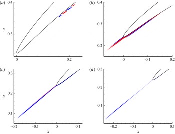
Figure 11. Contours of streamwise vorticity for the optimal initial perturbations in region ‘C’ at (a) $(\unicode[STIX]{x1D6FD},\unicode[STIX]{x1D70F})=(40\unicode[STIX]{x03C0},0.3)$
, (b)
$(\unicode[STIX]{x1D6FD},\unicode[STIX]{x1D70F})=(40\unicode[STIX]{x03C0},0.3)$
, (b) $(\unicode[STIX]{x1D6FD},\unicode[STIX]{x1D70F})=(120\unicode[STIX]{x03C0},0.3)$
, (c)
$(\unicode[STIX]{x1D6FD},\unicode[STIX]{x1D70F})=(120\unicode[STIX]{x03C0},0.3)$
, (c) $(\unicode[STIX]{x1D6FD},\unicode[STIX]{x1D70F})=(120\unicode[STIX]{x03C0},0.5)$
and (d)
$(\unicode[STIX]{x1D6FD},\unicode[STIX]{x1D70F})=(120\unicode[STIX]{x03C0},0.5)$
and (d) $(\unicode[STIX]{x1D6FD},\unicode[STIX]{x1D70F})=(120\unicode[STIX]{x03C0},0.6)$
, respectively, corresponding to points marked as ‘a’, ‘b’, ‘c’ and ‘d’ in figure 10.
$(\unicode[STIX]{x1D6FD},\unicode[STIX]{x1D70F})=(120\unicode[STIX]{x03C0},0.6)$
, respectively, corresponding to points marked as ‘a’, ‘b’, ‘c’ and ‘d’ in figure 10.
The optimal initial perturbations in region ‘C’ are shown in figure 11. At small values of $\unicode[STIX]{x1D70F}$
and
$\unicode[STIX]{x1D70F}$
and $\unicode[STIX]{x1D6FD}$
, specifically
$\unicode[STIX]{x1D6FD}$
, specifically $\unicode[STIX]{x1D70F}=0.3$
and
$\unicode[STIX]{x1D70F}=0.3$
and $\unicode[STIX]{x1D6FD}=40\unicode[STIX]{x03C0}$
with energy growth
$\unicode[STIX]{x1D6FD}=40\unicode[STIX]{x03C0}$
with energy growth $G=3.5\times 10^{2}$
, the optimal initial perturbation is located inside the boundary layer and is tilted against the shear to take advantage of the Orr mechanism, which realigns the optimal initial perturbation with the shear and amplifies it through the action of the pressure (figure 11
a). This Orr mechanism is dominant over small values of the target time
$G=3.5\times 10^{2}$
, the optimal initial perturbation is located inside the boundary layer and is tilted against the shear to take advantage of the Orr mechanism, which realigns the optimal initial perturbation with the shear and amplifies it through the action of the pressure (figure 11
a). This Orr mechanism is dominant over small values of the target time $\unicode[STIX]{x1D70F}<0.2$
.
$\unicode[STIX]{x1D70F}<0.2$
.
At higher spanwise wavenumbers, another form of the optimal initial perturbation is introduced, and it involves streamwise vorticity. At $\unicode[STIX]{x1D6FD}=120\unicode[STIX]{x03C0}$
and
$\unicode[STIX]{x1D6FD}=120\unicode[STIX]{x03C0}$
and $\unicode[STIX]{x1D70F}=0.3$
, the optimal perturbation is a combination of the tilted structure and streamwise vorticity (see figure 11
b). Increasing the target time,
$\unicode[STIX]{x1D70F}=0.3$
, the optimal perturbation is a combination of the tilted structure and streamwise vorticity (see figure 11
b). Increasing the target time, $\unicode[STIX]{x1D70F}$
, displaces the optimal perturbation upstream of the leading edge; the Orr mechanism vanishes, and only the streamwise vorticity remains (see figure 11
c,d).
$\unicode[STIX]{x1D70F}$
, displaces the optimal perturbation upstream of the leading edge; the Orr mechanism vanishes, and only the streamwise vorticity remains (see figure 11
c,d).
Based on figures 10 and 11, on the pressure surface, when the target time is short, the Orr mechanism is dominant and perturbations with lower spanwise wavenumber are most amplified as they are reoriented by the mean shear. At sufficiently large target times, the optimal initial perturbation starts upstream of the leading edge and takes the form of streamwise vorticity with high spanwise wavenumbers.

Figure 12. Contours of streamwise velocity for the outcome of the optimal perturbation in region ‘C’ at (a) $(\unicode[STIX]{x1D6FD},\unicode[STIX]{x1D70F},t)=(40\unicode[STIX]{x03C0},0.3,0.3)$
and (b)
$(\unicode[STIX]{x1D6FD},\unicode[STIX]{x1D70F},t)=(40\unicode[STIX]{x03C0},0.3,0.3)$
and (b) $(\unicode[STIX]{x1D6FD},\unicode[STIX]{x1D70F},t)=(120\unicode[STIX]{x03C0},0.5,0.5)$
.
$(\unicode[STIX]{x1D6FD},\unicode[STIX]{x1D70F},t)=(120\unicode[STIX]{x03C0},0.5,0.5)$
.
The two linear responses to the optimal perturbations are illustrated in figure 12. The first disturbance is tilted forward at $t=\unicode[STIX]{x1D70F}$
(see figure 12
a). The streamwise vorticity perturbation, on the other hand, generates streamwise velocity streaks with low streamwise and high spanwise wavenumbers (see figure 12
b).
$t=\unicode[STIX]{x1D70F}$
(see figure 12
a). The streamwise vorticity perturbation, on the other hand, generates streamwise velocity streaks with low streamwise and high spanwise wavenumbers (see figure 12
b).
Both the Orr amplification at low spanwise wavenumber, and the lift up at high spanwise wavenumber have been reported in a Blasius boundary-layer flow, although earlier analyses excluded the leading edge (Andersson et al. Reference Andersson, Berggren and Henningson1999; Monokrousos et al. Reference Monokrousos, Åkervik, Brandt and Henningson2010). Here, in contrast, the region upstream of the leading edge is included in the analysis. The present work is therefore the first investigation to demonstrate the origin of boundary-layer streaks when the finite thickness leading edge is fully resolved. It is worth noting that in this concave region ‘C’, no Görtler instability was observed in the present work or in the DNS by Zaki et al. (Reference Zaki, Wissink, Rodi and Durbin2010) where transition was initiated in response to forcing by free-stream turbulence.
In §§ 6.2 and 6.3, the nonlinear flow responses to the two types of optimal perturbations, namely the Orr distortions and the streamwise vortices, will be discussed. In addition to finite-amplitude effects, the nonlinear computations also capture the process of laminar-to-turbulence transition due to each type of disturbance.
6.2 The origin of
$\unicode[STIX]{x1D6EC}$
-structures

The results presented in § 6.1 are based on linearized analyses. In this section the nonlinear evolution and the subsequent laminar–turbulent transition are investigated using DNS, where the initial condition is a superposition of the base flow and a linearly optimal disturbance but with finite initial amplitude. We define a perturbation relative magnitude, denoted as $r$
, which is the ratio of the maximum initial perturbation velocity to the free-stream base-flow velocity. A typical disturbance, namely the optimal initial perturbation obtained at
$r$
, which is the ratio of the maximum initial perturbation velocity to the free-stream base-flow velocity. A typical disturbance, namely the optimal initial perturbation obtained at $\unicode[STIX]{x1D70F}=0.3$
and
$\unicode[STIX]{x1D70F}=0.3$
and $\unicode[STIX]{x1D6FD}=40\unicode[STIX]{x03C0}$
, is considered. To activate the nonlinear effects at an early time, a large relative magnitude of the perturbation, i.e.
$\unicode[STIX]{x1D6FD}=40\unicode[STIX]{x03C0}$
, is considered. To activate the nonlinear effects at an early time, a large relative magnitude of the perturbation, i.e. $r=0.1$
is applied. The spanwise domain size is set to
$r=0.1$
is applied. The spanwise domain size is set to $2\unicode[STIX]{x03C0}/(40\unicode[STIX]{x03C0})=0.05$
, in order to accommodate the initial perturbation as well as the higher harmonic modes, and 32 Fourier modes are evaluated in the span. In figure 13, the simulation domain is reproduced three times in the spanwise direction so that it matches the domain width in figure 6. For clarity, to reference a particular spanwise wavenumber
$2\unicode[STIX]{x03C0}/(40\unicode[STIX]{x03C0})=0.05$
, in order to accommodate the initial perturbation as well as the higher harmonic modes, and 32 Fourier modes are evaluated in the span. In figure 13, the simulation domain is reproduced three times in the spanwise direction so that it matches the domain width in figure 6. For clarity, to reference a particular spanwise wavenumber $\unicode[STIX]{x1D6FD}$
, we will refer to
$\unicode[STIX]{x1D6FD}$
, we will refer to $n$
, which is an integer number satisfying
$n$
, which is an integer number satisfying $\unicode[STIX]{x1D6FD}=40\unicode[STIX]{x03C0}n$
. In this definition, mode 0 represents the spanwise mean flow and mode 1 refers to the optimal initial perturbation.
$\unicode[STIX]{x1D6FD}=40\unicode[STIX]{x03C0}n$
. In this definition, mode 0 represents the spanwise mean flow and mode 1 refers to the optimal initial perturbation.

Figure 13. Iso-surfaces of streamwise perturbation velocity 0.05 (red) and $-0.05$
(blue) at (a)
$-0.05$
(blue) at (a) $t=0$
, (b)
$t=0$
, (b) $t=0.1$
, (c)
$t=0.1$
, (c) $t=0.4$
and (d)
$t=0.4$
and (d) $t=1$
, as obtained via DNS. The initial perturbation level is
$t=1$
, as obtained via DNS. The initial perturbation level is $r=0.1$
and the distribution is optimal at
$r=0.1$
and the distribution is optimal at $\unicode[STIX]{x1D6FD}=40\unicode[STIX]{x03C0}$
and
$\unicode[STIX]{x1D6FD}=40\unicode[STIX]{x03C0}$
and $\unicode[STIX]{x1D70F}=0.3$
in region ‘C’.
$\unicode[STIX]{x1D70F}=0.3$
in region ‘C’.
In the 3-D view, the initial perturbation (figure 13
a) is rotated from its initial tilt against the shear to a forward tilt and subsequently develops $\unicode[STIX]{x1D6EC}$
structures at
$\unicode[STIX]{x1D6EC}$
structures at $t=0.1$
(figure 13
b). The streamwise wavelength of the
$t=0.1$
(figure 13
b). The streamwise wavelength of the $\unicode[STIX]{x1D6EC}$
structures is of the same order as that of the unstable modes associated with TS waves. The spanwise length of the
$\unicode[STIX]{x1D6EC}$
structures is of the same order as that of the unstable modes associated with TS waves. The spanwise length of the $\unicode[STIX]{x1D6EC}$
structures is approximately five times the boundary-layer thickness, similar to the results by Liu et al. (Reference Liu, Zaki and Durbin2008) for their ‘mode 2’ case for the interaction of streaks and TS waves. At
$\unicode[STIX]{x1D6EC}$
structures is approximately five times the boundary-layer thickness, similar to the results by Liu et al. (Reference Liu, Zaki and Durbin2008) for their ‘mode 2’ case for the interaction of streaks and TS waves. At $t=0.4$
, the
$t=0.4$
, the $\unicode[STIX]{x1D6EC}$
structures are further stretched to form hairpin vortices (figure 13
c) and the perturbation energy is transferred to shorter waves in the span. Finally, a late stage of transition is observed in figure 13(d). This laminar–turbulent transition scenario can be divided into two steps: a linear transient growth owing to the Orr mechanism and the nonlinear breakdown of the ensuing
$\unicode[STIX]{x1D6EC}$
structures are further stretched to form hairpin vortices (figure 13
c) and the perturbation energy is transferred to shorter waves in the span. Finally, a late stage of transition is observed in figure 13(d). This laminar–turbulent transition scenario can be divided into two steps: a linear transient growth owing to the Orr mechanism and the nonlinear breakdown of the ensuing $\unicode[STIX]{x1D6EC}$
structures. The nonlinear stage features energy transfer from the dominant mode to shorter spanwise waves.
$\unicode[STIX]{x1D6EC}$
structures. The nonlinear stage features energy transfer from the dominant mode to shorter spanwise waves.

Figure 14. Energy of various spanwise Fourier modes at initial perturbation level (a) $r=0.001$
, (b)
$r=0.001$
, (b) $r=0.01$
and (c)
$r=0.01$
and (c) $r=0.1$
. The initial perturbation is optimal at
$r=0.1$
. The initial perturbation is optimal at $\unicode[STIX]{x1D6FD}=40\unicode[STIX]{x03C0}$
and
$\unicode[STIX]{x1D6FD}=40\unicode[STIX]{x03C0}$
and $\unicode[STIX]{x1D70F}=0.3$
in region ‘C’.
$\unicode[STIX]{x1D70F}=0.3$
in region ‘C’.
In order to examine the energy transfer between Fourier waves, the time evolution of the spectra is plotted in figure 14. For all three magnitudes of the initial perturbation, there is no exponential growth of any of the harmonics, which precludes the possibility of secondary instability via parametric resonance. In addition, the energy of spanwise shorter waves is almost uniformly smaller than that of longer ones. These results demonstrate that the energy growth is nonlinear via energy transfer. At the highest perturbation amplitude (figure 15
c), mode 2 overtakes mode 1 at $t\approx 0.1$
, which corresponds to the generation of the
$t\approx 0.1$
, which corresponds to the generation of the $\unicode[STIX]{x1D6EC}$
structures in figure 13(b).
$\unicode[STIX]{x1D6EC}$
structures in figure 13(b).

Figure 15. Iso-surfaces of positive (red) and negative (blue) streamwise perturbation velocity at $t=0.1$
and perturbation level (a)
$t=0.1$
and perturbation level (a) $r=0.001$
, (b)
$r=0.001$
, (b) $r=0.01$
and (c)
$r=0.01$
and (c) $r=0.1$
, as obtained via DNS. The horizontal and vertical directions in the plots are aligned with the streamwise and spanwise directions, respectively.
$r=0.1$
, as obtained via DNS. The horizontal and vertical directions in the plots are aligned with the streamwise and spanwise directions, respectively.
To better illustrate the formation of the $\unicode[STIX]{x1D6EC}$
structures, the perturbations that result from three different initial magnitudes,
$\unicode[STIX]{x1D6EC}$
structures, the perturbations that result from three different initial magnitudes, $r=0.001$
,
$r=0.001$
, $0.01$
and
$0.01$
and $0.1$
, are compared at
$0.1$
, are compared at $t=0.1$
in figure 15. For the smallest initial amplitude,
$t=0.1$
in figure 15. For the smallest initial amplitude, $r=0.001$
, the perturbation is predominantly monochromatic in the span. At the intermediate amplitude,
$r=0.001$
, the perturbation is predominantly monochromatic in the span. At the intermediate amplitude, $r=0.01$
, the positive streamwise velocity perturbations cover a larger area than the negative ones, which is a manifestation of quadratic-type nonlinearity being active. At the highest amplitude,
$r=0.01$
, the positive streamwise velocity perturbations cover a larger area than the negative ones, which is a manifestation of quadratic-type nonlinearity being active. At the highest amplitude, $r=0.1$
, the
$r=0.1$
, the $\unicode[STIX]{x1D6EC}$
structures are clearly visible.
$\unicode[STIX]{x1D6EC}$
structures are clearly visible.

Figure 16. Iso-surfaces of filtered streamwise perturbation velocity 0.05 (red) and $-0.05$
(blue) at perturbation level
$-0.05$
(blue) at perturbation level $r=0.1$
and
$r=0.1$
and $t=0.1$
. (a) Fourier modes 0 and 1; (b) Fourier modes 0, 1 and 2; (c) Fourier modes 0, 1, 2 and 3. The horizontal and vertical directions in the plots are aligned with the streamwise and spanwise directions, respectively.
$t=0.1$
. (a) Fourier modes 0 and 1; (b) Fourier modes 0, 1 and 2; (c) Fourier modes 0, 1, 2 and 3. The horizontal and vertical directions in the plots are aligned with the streamwise and spanwise directions, respectively.
The nonlinear nature of the $\unicode[STIX]{x1D6EC}$
structures in figure 15(c) is further studied by filtering the high wavenumber components (see figure 16). By only retaining modes 0 and 1 (figure 16
a), the perturbation field appreciably deviates from the unfiltered results. On the other hand, the superposition of modes 0, 1 and 2 (figure 16
b) is almost identical to the unfiltered perturbation, as is the sum of modes 0, 1, 2 and 3 (figure 16
c). These observations indicate that the
$\unicode[STIX]{x1D6EC}$
structures in figure 15(c) is further studied by filtering the high wavenumber components (see figure 16). By only retaining modes 0 and 1 (figure 16
a), the perturbation field appreciably deviates from the unfiltered results. On the other hand, the superposition of modes 0, 1 and 2 (figure 16
b) is almost identical to the unfiltered perturbation, as is the sum of modes 0, 1, 2 and 3 (figure 16
c). These observations indicate that the $\unicode[STIX]{x1D6EC}$
structures are mostly due to mode 2, which is the direct nonlinear interaction of the dominant mode with itself.
$\unicode[STIX]{x1D6EC}$
structures are mostly due to mode 2, which is the direct nonlinear interaction of the dominant mode with itself.
6.3 The formation of streaks and bypass transition

Figure 17. (a) Iso-surfaces of streamwise perturbation vorticity 10 (red) and $-10$
(blue) at
$-10$
(blue) at $t=0$
; (b), (c) and (d) iso-surfaces of streamwise velocity perturbation
$t=0$
; (b), (c) and (d) iso-surfaces of streamwise velocity perturbation $-0.05$
(blue) and 0.05 (red) at
$-0.05$
(blue) and 0.05 (red) at $t=0.1$
,
$t=0.1$
, $t=0.5$
and
$t=0.5$
and $t=0.8$
, respectively. The initial perturbation is optimal at
$t=0.8$
, respectively. The initial perturbation is optimal at $\unicode[STIX]{x1D70F}=0.5$
and
$\unicode[STIX]{x1D70F}=0.5$
and $\unicode[STIX]{x1D6FD}=120\unicode[STIX]{x03C0}$
, and has a relative magnitude
$\unicode[STIX]{x1D6FD}=120\unicode[STIX]{x03C0}$
, and has a relative magnitude $r=0.08$
, as will be used in all the following plots if not otherwise stated.
$r=0.08$
, as will be used in all the following plots if not otherwise stated.
Similar to § 6.2, in this section the optimal initial perturbation with $\unicode[STIX]{x1D70F}=0.5$
and
$\unicode[STIX]{x1D70F}=0.5$
and $\unicode[STIX]{x1D6FD}=120\unicode[STIX]{x03C0}$
, is superimposed onto the base flow. A nonlinear initial perturbation amplitude of
$\unicode[STIX]{x1D6FD}=120\unicode[STIX]{x03C0}$
, is superimposed onto the base flow. A nonlinear initial perturbation amplitude of $r=0.08$
is considered first, in order to examine the full transition process. Subsequently, other initial perturbation levels will also be discussed. The development of the streamwise disturbance velocity is shown in figure 17. The spanwise domain size is 0.05 and is resolved using 32 spanwise Fourier modes. Again for clarity, the results are reproduced in the spanwise direction three times.
$r=0.08$
is considered first, in order to examine the full transition process. Subsequently, other initial perturbation levels will also be discussed. The development of the streamwise disturbance velocity is shown in figure 17. The spanwise domain size is 0.05 and is resolved using 32 spanwise Fourier modes. Again for clarity, the results are reproduced in the spanwise direction three times.
The perturbation has a low streamwise wavenumber, and is initially localized upstream of the blade leading edge (figure 17
a). The initial disturbance triggers the formation of streamwise velocity streaks via the lift-up mechanism (figure 17
b). These streaks are further amplified, while the high- (low-) speed ones move towards (away from) the blade surface (figure 17
c). Finally the streaks break down to turbulence with the apparent formation of hairpin vortices (figure 17
d). The generation, dynamics and secondary instability of the streaks are examined in detail in each of the subsequent sections (§§ 6.3.1–6.3.3). Unless otherwise stated, the optimal initial perturbation for $\unicode[STIX]{x1D6FD}=120\unicode[STIX]{x03C0}$
and
$\unicode[STIX]{x1D6FD}=120\unicode[STIX]{x03C0}$
and $\unicode[STIX]{x1D70F}=0.5$
is adopted, with relative magnitude
$\unicode[STIX]{x1D70F}=0.5$
is adopted, with relative magnitude $r=0.08$
.
$r=0.08$
.
6.3.1 Nonlinear streaks
The streamwise velocity perturbation at various downstream locations is plotted in figure 18. The high- and low-speed streaks appear periodically at $x=0.1$
. Their initial amplification is due to the linear lift-up mechanism, which can be traced to the action of the streamwise vorticity perturbation onto the base-flow shear. Downstream the streamwise vorticity perturbation acts on the streaks themselves, which is a nonlinear effect (since both the vorticity and the streaks are perturbation quantities). This nonlinear interaction alters the spanwise harmonic appearance of the streaks into trapezoidal shapes (figure 18
b). Farther downstream (figure 18
c), the nonlinear lift up displaces the streaks in the wall-normal direction, with the low-speed structures overhanging the high-speed ones. This configuration is prone to secondary instabilities, which are visible in figure 18(e) and will be discussed in detail in § 6.3.3. The instability can be classified as an inner mode, which is symmetric with respect to the streak and can originate in the overlap region between the high- and low-speed streaks (Vaughan & Zaki Reference Vaughan and Zaki2011; Hack & Zaki Reference Hack and Zaki2014). Another instability, featuring asymmetric deformation of the upper part of low-speed streaks, or the outer mode, is clearly observed in figure 18(f). These streak instabilities are discussed in detail in § 6.3.3.
$x=0.1$
. Their initial amplification is due to the linear lift-up mechanism, which can be traced to the action of the streamwise vorticity perturbation onto the base-flow shear. Downstream the streamwise vorticity perturbation acts on the streaks themselves, which is a nonlinear effect (since both the vorticity and the streaks are perturbation quantities). This nonlinear interaction alters the spanwise harmonic appearance of the streaks into trapezoidal shapes (figure 18
b). Farther downstream (figure 18
c), the nonlinear lift up displaces the streaks in the wall-normal direction, with the low-speed structures overhanging the high-speed ones. This configuration is prone to secondary instabilities, which are visible in figure 18(e) and will be discussed in detail in § 6.3.3. The instability can be classified as an inner mode, which is symmetric with respect to the streak and can originate in the overlap region between the high- and low-speed streaks (Vaughan & Zaki Reference Vaughan and Zaki2011; Hack & Zaki Reference Hack and Zaki2014). Another instability, featuring asymmetric deformation of the upper part of low-speed streaks, or the outer mode, is clearly observed in figure 18(f). These streak instabilities are discussed in detail in § 6.3.3.

Figure 18. Contours of streamwise perturbation velocity at $t=0.52$
and
$t=0.52$
and $x=0.1$
, 0.15, 0.2, 0.25, 0.27 and 0.285 for (a), (b), (c), (d), (e) and (f), respectively. The dotted lines denote the border between high-speed and low-speed streaks. Vertical and horizontal axes represent
$x=0.1$
, 0.15, 0.2, 0.25, 0.27 and 0.285 for (a), (b), (c), (d), (e) and (f), respectively. The dotted lines denote the border between high-speed and low-speed streaks. Vertical and horizontal axes represent $y$
and
$y$
and $z$
, respectively.
$z$
, respectively.

Figure 19. Side view of iso-surfaces of streamwise velocity $-0.05$
(blue) and 0.05 (red) at
$-0.05$
(blue) and 0.05 (red) at $t=0.6$
and perturbation magnitude (a)
$t=0.6$
and perturbation magnitude (a) $r=0.004$
, (b)
$r=0.004$
, (b) $r=0.04$
and (c)
$r=0.04$
and (c) $r=0.08$
.
$r=0.08$
.
The above observations are based on results from simulations with initial perturbation magnitude equal to 0.08. The streaks amplify in response to three initial amplitudes are compared in figure 19. As the initial amplitude is increased, the streak becomes energetic, and the low-speed ones are increasingly lifted away from the wall. In figure 19(b), when the initial perturbation magnitude reaches 0.04, the streaks exhibit signs of the onset of secondary instabilities, which become much more evident at higher amplitudes (figure 19 c).

Figure 20. Schematic plot of the linear and nonlinear lift-up mechanisms. The resulting perturbed shear flow is plotted on the right. Symbols ‘ $+$
’ and ‘
$+$
’ and ‘ $-$
’ denote the sign of the streaks; the dashed lines represent the streamwise vorticity, with the direction denoted by arrows.
$-$
’ denote the sign of the streaks; the dashed lines represent the streamwise vorticity, with the direction denoted by arrows.
A schematic of the linear and nonlinear stages of the streak amplification are shown in figure 20. The optimal initial perturbations are streamwise vortices which displace, or lift up, the mean flow and create low- and high-speed streaks. In the linear limit of infinitesimal disturbance amplitudes, the interaction of the streamwise vorticity and streaks is negligible. However, when the initial magnitude of the perturbation is sufficiently large, the streamwise vorticity acts on the streaks, and induces a vertical displacement and a lateral deformation. The nonlinear streaks distort the mean shear profile. The distortion is an excess velocity near the wall and a deficit higher in the boundary layer, which is consistent with previous studies (Jacobs & Durbin Reference Jacobs and Durbin2001; Brandt et al. Reference Brandt, Cossu, Chomaz, Huerre and Henningson2003; Nolan & Zaki Reference Nolan and Zaki2013).
6.3.2 Streak development

Figure 21. Iso-surfaces of streamwise perturbation velocity 0.05 (a,c,e,g) and $-0.05$
(b,d,f,h) at
$-0.05$
(b,d,f,h) at $t=0.52$
,
$t=0.52$
, $0.58$
and
$0.58$
and $0.66$
from top to bottom. The first row is lateral view with the dotted lines denoting
$0.66$
from top to bottom. The first row is lateral view with the dotted lines denoting $x=0.27$
; all the following rows are top view.
$x=0.27$
; all the following rows are top view.
The low- and high-speed streaks introduce spanwise and wall-normal inflection points in the velocity profile, and render it unstable. Two classes of secondary instabilities of the streaky base state have been defined: an outer instability and an inner instability (Vaughan & Zaki Reference Vaughan and Zaki2011; Hack & Zaki Reference Hack and Zaki2014). The former affects the lifted low-speed streaks, and the latter is due to the near-wall inflection point that can form at the overlap between the low- and high-speed streaks. It is noted that a spanwise inflectional distortion of the velocity profile can also promote secondary instability and breakdown to turbulence (Goldstein, Leib & Cowley Reference Goldstein, Leib and Cowley1992). In order to highlight the differences between the two classes of secondary instabilities, the low- and high-speed streaks are shown separately in figure 21. The high-speed streaks are deformed in a manner suggestive of varicose instability. In the meantime, the lifted low-speed streaks are meandering in a sinuous motion. At $t=0.58$
, the further development of the unstable high-speed streaks leads to the formation of the
$t=0.58$
, the further development of the unstable high-speed streaks leads to the formation of the $\unicode[STIX]{x1D6EC}$
structures (figure 21
e). At
$\unicode[STIX]{x1D6EC}$
structures (figure 21
e). At $t=0.66$
(figure 21
g), they start to locally break down to turbulence. This process features the formation of hairpin vortices from the stretching of the
$t=0.66$
(figure 21
g), they start to locally break down to turbulence. This process features the formation of hairpin vortices from the stretching of the $\unicode[STIX]{x1D6EC}$
structures, as previously discussed in connection with figure 17(d). The low-speed streaks, on the other hand, continue to meander, and the spanwise wavenumber of the secondary instability is subharmonic relative to the underlying streaks (see figure 21
h).
$\unicode[STIX]{x1D6EC}$
structures, as previously discussed in connection with figure 17(d). The low-speed streaks, on the other hand, continue to meander, and the spanwise wavenumber of the secondary instability is subharmonic relative to the underlying streaks (see figure 21
h).

Figure 22. Contours of streamwise perturbation velocity at $x=0.27$
and
$x=0.27$
and $t=0.52$
for (a) mode 0, (b) mode 1, (c) mode 2 and (d) mode 3. The dotted lines denote the border between high-speed and low-speed streaks. Vertical and horizontal axes represent
$t=0.52$
for (a) mode 0, (b) mode 1, (c) mode 2 and (d) mode 3. The dotted lines denote the border between high-speed and low-speed streaks. Vertical and horizontal axes represent $y$
and
$y$
and $z$
, respectively.
$z$
, respectively.
The velocity fields associated with various spanwise Fourier modes are shown in figure 22. The distorted base flow (mode 0) and the fundamental streak wavenumber (mode 3) have the highest energy. Modes 1 and 2 are concentrated around the location of low-speed streaks and are related to the outer instability; they will be shown to become energetic late in the transition process (see figure 23).

Figure 23. Energy of various spanwise Fourier modes at perturbation magnitude (a) $r=0.0004$
, (b)
$r=0.0004$
, (b) $r=0.004$
, (c)
$r=0.004$
, (c) $r=0.04$
and (d)
$r=0.04$
and (d) $r=0.08$
. The symbols used in four plots are the same, as presented in (d).
$r=0.08$
. The symbols used in four plots are the same, as presented in (d).
To quantitatively characterize the development of streaks, the energy spectral density is plotted in figure 23. The four panels correspond to different initial optimal disturbance amplitudes. The base spanwise wavenumber of the streaks (mode 3) and its first harmonic (mode 6) are dominant. The remaining modes, and in particular, the high wavenumbers (e.g. mode 8), exhibit strong transient growth over short time intervals, followed by exponential growth, signalling the onset of bypass breakdown to turbulence. Modes which are not harmonics of the fundamental streak wavenumber are initialized by round-off errors with energy of the order of $10^{-37}$
and amplify through interactions with the harmonic waves. The two stages of the streak instability (transient followed by exponential growth) are examined in detail using a secondary perturbation analysis in the following section.
$10^{-37}$
and amplify through interactions with the harmonic waves. The two stages of the streak instability (transient followed by exponential growth) are examined in detail using a secondary perturbation analysis in the following section.
6.3.3 Secondary instability

Figure 24. Streamwise velocity profile extracted on the pressure side at (a) $x=0.1$
and
$x=0.1$
and $t=0.05$
, and (b)
$t=0.05$
, and (b) $x=0.27$
and
$x=0.27$
and $t=0.52$
;
$t=0.52$
; $z$
and
$z$
and $y_{n}$
denote the spanwise and wall-normal directions, respectively.
$y_{n}$
denote the spanwise and wall-normal directions, respectively.
To study the early stage of the streak instability, which features transient growth of modes with high spanwise wavenumbers, the velocity profile near the leading edge at $x=0.1$
and
$x=0.1$
and $t=0.05$
is adopted as the base state, as shown in figure 24(a). Owing to the presence of streaks, the streamwise velocity profile undulates slightly along the spanwise dimension, which has non-negligible effects on the results of the analysis (as will be illustrated in figure 26). To examine the late stage secondary instability, which features exponential growth of modes with low spanwise wavenumbers, the velocity profile is also extracted at
$t=0.05$
is adopted as the base state, as shown in figure 24(a). Owing to the presence of streaks, the streamwise velocity profile undulates slightly along the spanwise dimension, which has non-negligible effects on the results of the analysis (as will be illustrated in figure 26). To examine the late stage secondary instability, which features exponential growth of modes with low spanwise wavenumbers, the velocity profile is also extracted at $x=0.27$
and
$x=0.27$
and $t=0.52$
. As shown in figure 24(b), at this location and time, the high-amplitude low-speed streaks have been lifted above the high-speed ones.
$t=0.52$
. As shown in figure 24(b), at this location and time, the high-amplitude low-speed streaks have been lifted above the high-speed ones.

Figure 25. Logarithm of the energy amplification, based on the velocity profile extracted at $x=0.1$
and
$x=0.1$
and $t=0.05$
on the pressure side;
$t=0.05$
on the pressure side; $k$
is the streamwise wavenumber. The optimal initial perturbations at points ‘
$k$
is the streamwise wavenumber. The optimal initial perturbations at points ‘ $\mathbf{a}$
’, ‘
$\mathbf{a}$
’, ‘ $\mathbf{b}$
’, ‘
$\mathbf{b}$
’, ‘ $\mathbf{c}$
’ and ‘
$\mathbf{c}$
’ and ‘ $\mathbf{d}$
’ are illustrated in figure 26(a), (b), (c) and (d), respectively.
$\mathbf{d}$
’ are illustrated in figure 26(a), (b), (c) and (d), respectively.

Figure 26. Contours of the streamwise velocity of secondary optimal initial perturbations (left) and outcomes (right) at (a) $(\unicode[STIX]{x1D70F},k)=(0.01,150\unicode[STIX]{x03C0})$
, (b)
$(\unicode[STIX]{x1D70F},k)=(0.01,150\unicode[STIX]{x03C0})$
, (b) $(\unicode[STIX]{x1D70F},k)=(0.03,120\unicode[STIX]{x03C0})$
, (c)
$(\unicode[STIX]{x1D70F},k)=(0.03,120\unicode[STIX]{x03C0})$
, (c) $(\unicode[STIX]{x1D70F},k)=(0.05,90\unicode[STIX]{x03C0})$
and (d)
$(\unicode[STIX]{x1D70F},k)=(0.05,90\unicode[STIX]{x03C0})$
and (d) $(\unicode[STIX]{x1D70F},k)=(0.1,50\unicode[STIX]{x03C0})$
. The base flow is extracted from the cross-section at
$(\unicode[STIX]{x1D70F},k)=(0.1,50\unicode[STIX]{x03C0})$
. The base flow is extracted from the cross-section at $x=0.1$
and
$x=0.1$
and $t=0.05$
. The streamwise wavenumber
$t=0.05$
. The streamwise wavenumber $k$
is selected to maximize the transient growth.
$k$
is selected to maximize the transient growth.
The secondary transient growth based on the upstream profile is shown in figure 25. We only considered time interval $\unicode[STIX]{x1D70F}\leqslant 0.1$
, since the state is assumed to be frozen and therefore the analysis is only valid over short times. With these restrictions, short streamwise waves are the most dominant.
$\unicode[STIX]{x1D70F}\leqslant 0.1$
, since the state is assumed to be frozen and therefore the analysis is only valid over short times. With these restrictions, short streamwise waves are the most dominant.
The secondary optimal perturbations and the associated flow responses at various final times are shown in figure 26. The streamwise wavenumbers are selected to maximize the transient growth. At small values of $\unicode[STIX]{x1D70F}$
, the scale of the perturbation is small. As
$\unicode[STIX]{x1D70F}$
, the scale of the perturbation is small. As $\unicode[STIX]{x1D70F}$
increases, the optimal perturbation becomes larger and tends to the spanwise width of the streaks (mode 3, or three waves in the domain). This observation suggests that the streaky shear profile supports transient growth of high-spanwise-wavenumber perturbations, which is consistent with the results in figure 23.
$\unicode[STIX]{x1D70F}$
increases, the optimal perturbation becomes larger and tends to the spanwise width of the streaks (mode 3, or three waves in the domain). This observation suggests that the streaky shear profile supports transient growth of high-spanwise-wavenumber perturbations, which is consistent with the results in figure 23.
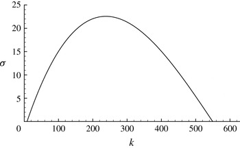
Figure 27. Growth rate ( $\unicode[STIX]{x1D70E}$
) of secondary instability based on the streaky profile extracted at
$\unicode[STIX]{x1D70E}$
) of secondary instability based on the streaky profile extracted at $x=0.27$
and
$x=0.27$
and $t=0.52$
.
$t=0.52$
.

Figure 28. Most unstable secondary modes at streamwise wavenumber (a) $k=10\unicode[STIX]{x03C0}$
, (b)
$k=10\unicode[STIX]{x03C0}$
, (b) $k=20\unicode[STIX]{x03C0}$
, (c)
$k=20\unicode[STIX]{x03C0}$
, (c) $k=50\unicode[STIX]{x03C0}$
and (d)
$k=50\unicode[STIX]{x03C0}$
and (d) $k=85\unicode[STIX]{x03C0}$
. The base flow is extracted at
$k=85\unicode[STIX]{x03C0}$
. The base flow is extracted at $t=0.52$
and
$t=0.52$
and $x=0.27$
. The contour flood denotes high-speed (red) and low-speed (blue) streaks in the base flow. Solid and dashed contour lines represent positive and negative contour levels for the secondary mode.
$x=0.27$
. The contour flood denotes high-speed (red) and low-speed (blue) streaks in the base flow. Solid and dashed contour lines represent positive and negative contour levels for the secondary mode.
The secondary instability of the streaky profile (see figure 24
b) is presented in figure 27. The growth rate reaches a maximum value that slightly exceeds $\unicode[STIX]{x1D70E}=20$
at streamwise wavenumber
$\unicode[STIX]{x1D70E}=20$
at streamwise wavenumber $k=85\unicode[STIX]{x03C0}$
, which is much higher than the wavenumber of the streak meandering motion observed in figure 21. The shapes of the most unstable modes are illustrated in figure 28. At
$k=85\unicode[STIX]{x03C0}$
, which is much higher than the wavenumber of the streak meandering motion observed in figure 21. The shapes of the most unstable modes are illustrated in figure 28. At $k=10\unicode[STIX]{x03C0}$
, the most unstable mode includes a symmetric part around the border of high- and low-speed streaks, which resembles an inner instability, and an asymmetric part near the free-stream edge of the low-speed streaks (outer mode). As
$k=10\unicode[STIX]{x03C0}$
, the most unstable mode includes a symmetric part around the border of high- and low-speed streaks, which resembles an inner instability, and an asymmetric part near the free-stream edge of the low-speed streaks (outer mode). As $k$
increases, the instability tends more to the symmetric inner mode while the outer component diminishes. At
$k$
increases, the instability tends more to the symmetric inner mode while the outer component diminishes. At $k=85\unicode[STIX]{x03C0}$
, where the instability has the highest growth rate, the mode is localized to particular streaks – a result consistent with the previous work by Hack & Zaki (Reference Hack and Zaki2014) who predicted the localized secondary instability that precedes breakdown to turbulence in bypass transition.
$k=85\unicode[STIX]{x03C0}$
, where the instability has the highest growth rate, the mode is localized to particular streaks – a result consistent with the previous work by Hack & Zaki (Reference Hack and Zaki2014) who predicted the localized secondary instability that precedes breakdown to turbulence in bypass transition.
In summary, at the leading edge the streaky flow supports transient energy growth of perturbations with high spanwise wavenumbers. Further downstream, secondary exponential instability of the streaks dominates. At low streamwise wavenumbers, the secondary instability consists of both inner and outer modes. The latter one vanishes at high streamwise wavenumbers, and the inner instability prevails.
7 Conclusion
The flow around a NACA 65 airfoil in a compressor passage is studied using both modal and non-modal stability analyses, and DNS. The chord Reynolds number is fixed at $138\,500$
, and the computational set-up and accuracy were based on the earlier DNS study by Zaki et al. (Reference Zaki, Wissink, Rodi and Durbin2010).
$138\,500$
, and the computational set-up and accuracy were based on the earlier DNS study by Zaki et al. (Reference Zaki, Wissink, Rodi and Durbin2010).
The flow on the suction side downstream of the separation bubble is found to be most sensitive to perturbations. The global optimal initial perturbation has spanwise wavenumber $\unicode[STIX]{x1D6FD}=300\unicode[STIX]{x03C0}$
and its energy amplifies up to eight orders of magnitude within the shedding vortices. Due to the reverse base flow, the disturbance advects upstream into the braid region for another round of amplification. The repeated cycles of noise amplification induce a reoccurring transition process in DNS.
$\unicode[STIX]{x1D6FD}=300\unicode[STIX]{x03C0}$
and its energy amplifies up to eight orders of magnitude within the shedding vortices. Due to the reverse base flow, the disturbance advects upstream into the braid region for another round of amplification. The repeated cycles of noise amplification induce a reoccurring transition process in DNS.
In order to highlight the perturbation dynamics in other regions of interest, weighted transient growth analyses were adopted to localize perturbation growth in space. On the suction side upstream of the secondary bubble, the optimal initial perturbation is tilted against the shear and is amplified to an outcome that resembles discrete TS modes. Owing to the reverse base flow, a much longer duration than the optimal target time is required to recover the unperturbed state.
On the pressure side, two types of optimal initial perturbations are obtained. One has low spanwise wavenumber $\unicode[STIX]{x1D6FD}=40\unicode[STIX]{x03C0}$
and is initially tilted against the mean shear. In DNS, this perturbation amplifies as it is advected and reoriented by the mean flow. When the magnitude of the perturbation becomes sufficiently large,
$\unicode[STIX]{x1D6FD}=40\unicode[STIX]{x03C0}$
and is initially tilted against the mean shear. In DNS, this perturbation amplifies as it is advected and reoriented by the mean flow. When the magnitude of the perturbation becomes sufficiently large, $\unicode[STIX]{x1D6EC}$
structures appear and are stretched to hairpin vortices before breaking down to turbulence. In this transition scenario, transient energy growth and nonlinear effects are observed while absolute instabilities are absent.
$\unicode[STIX]{x1D6EC}$
structures appear and are stretched to hairpin vortices before breaking down to turbulence. In this transition scenario, transient energy growth and nonlinear effects are observed while absolute instabilities are absent.
Another type of optimal initial perturbation has higher spanwise wavenumber, $\unicode[STIX]{x1D6FD}=120\unicode[STIX]{x03C0}$
and is in the form of streamwise vortices. By increasing the value of the final time and only considering perturbation growth around the leading edge, the optimal initial perturbation is localized upstream of the leading edge, which was not possible in earlier studies that excluded the leading-edge region from the analysis. The initial disturbance generates high- and low-speed streaks through a linear ‘lift-up’ mechanism. These linear streaks are spanwise periodic.
$\unicode[STIX]{x1D6FD}=120\unicode[STIX]{x03C0}$
and is in the form of streamwise vortices. By increasing the value of the final time and only considering perturbation growth around the leading edge, the optimal initial perturbation is localized upstream of the leading edge, which was not possible in earlier studies that excluded the leading-edge region from the analysis. The initial disturbance generates high- and low-speed streaks through a linear ‘lift-up’ mechanism. These linear streaks are spanwise periodic.
In DNS, when the perturbation magnitude is sufficiently large, the spanwise vortices act on the streaks and lift the low-speed streaks above the high-speed ones. Since both the vortices and the streaks are perturbations, this mechanism is nonlinear. Such a configuration is prone to instabilities and both inner and outer modes. The inner mode appears at the boundary between high- and low-speed streaks. The outer modes, which manifest as a meandering motion of the low-speed streaks, was subharmonic in the span. Based on the secondary instability analysis, both the inner and outer modes coexist at low streamwise wavenumbers, while the latter one vanishes at higher streamwise numbers.
The present work demonstrates that linear modal and non-modal analyses and DNS can shed light on transition phenomena in complex configurations, such as flow over the compressor blade considered herein. By localizing the analysis, we have highlighted the most relevant disturbance amplification processes in various regions of the flow domain, and by aid of DNS the nonlinear lift-up mechanism was explained.
Acknowledgements
This work made use of the facilities of NCI under the project d77 and N8 HPC. X.M. would like to acknowledge financial support under Engineering and Physical Sciences Research Council (EPSRC) grant EP/M025039/1. S.J.S. and T.A.Z. acknowledge the support of EPSRC grant EP/H050507/1. H.M.B. and X.M. acknowledge the support of ARC grant DP1094851.
Appendix A. Validation of the spatially weighted transient growth
Owing to the application of the weight function $F$
, which is a regularized step function that is approximated in the computation using Lagrange polynomials, the adjoint variables can be initialized by a non-solenoidal condition as shown in figure 8. To validate these calculations, we compared the optimal energy growth
$F$
, which is a regularized step function that is approximated in the computation using Lagrange polynomials, the adjoint variables can be initialized by a non-solenoidal condition as shown in figure 8. To validate these calculations, we compared the optimal energy growth $G$
with the energy growth of individual optimal initial perturbations, denoted as
$G$
with the energy growth of individual optimal initial perturbations, denoted as $G_{i}$
(figure 29). Here
$G_{i}$
(figure 29). Here $G$
is obtained by applying an Arnoldi method to a Krylov sequence as discussed in § 2, and
$G$
is obtained by applying an Arnoldi method to a Krylov sequence as discussed in § 2, and
 $$\begin{eqnarray}G_{i}=\frac{(F{\mathcal{A}}\hat{\boldsymbol{u}}(0),F{\mathcal{A}}\hat{\boldsymbol{u}}(0))}{(\hat{\boldsymbol{u}}(0),\hat{\boldsymbol{u}}(0))}\end{eqnarray}$$
is obtained by evolving the optimal initial perturbation using the linearized NS equations. Therefore the non-solenoidal field appears in the calculation of $G$
, but not in that of
$G$
, but not in that of $G_{i}$
; the divergence-free condition is imposed at each time step implicitly when integrating the governing equations (Karniadakis et al.
Reference Karniadakis, Israeli and Orszag1991). The optimal transient growth curve acts as an envelope of each individual energy growth curve, and intersects with individual curves at
$G_{i}$
; the divergence-free condition is imposed at each time step implicitly when integrating the governing equations (Karniadakis et al.
Reference Karniadakis, Israeli and Orszag1991). The optimal transient growth curve acts as an envelope of each individual energy growth curve, and intersects with individual curves at $t=\unicode[STIX]{x1D70F}$
. This method has been widely used to validate the optimal perturbation calculations (Blackburn et al.
Reference Blackburn, Barkley and Sherwin2008; Mao, Blackburn & Sherwin Reference Mao, Blackburn and Sherwin2012). The agreement between
$t=\unicode[STIX]{x1D70F}$
. This method has been widely used to validate the optimal perturbation calculations (Blackburn et al.
Reference Blackburn, Barkley and Sherwin2008; Mao, Blackburn & Sherwin Reference Mao, Blackburn and Sherwin2012). The agreement between $G_{i}$
and
$G_{i}$
and $G$
indicates that the non-solenoidal condition used to initialize the adjoint equation does not change the optimality of the results reported in this work. A convergence test indicated that with the present definition of
$G$
indicates that the non-solenoidal condition used to initialize the adjoint equation does not change the optimality of the results reported in this work. A convergence test indicated that with the present definition of $F$
, the perturbation growth converges to three significant figures.
$F$
, the perturbation growth converges to three significant figures.

Figure 29. Validation of transient growth in region ‘B’ at $\unicode[STIX]{x1D6FD}=0$
.
$\unicode[STIX]{x1D6FD}=0$
. $G$
(see (2.4)) is the optimal weighted transient growth obtained from the Arnoldi method.
$G$
(see (2.4)) is the optimal weighted transient growth obtained from the Arnoldi method. $G_{i}$
(see (A 1)) denotes the weighted energy growth of an individual optimal initial perturbation is obtained by integrating the linearized NS equation.
$G_{i}$
(see (A 1)) denotes the weighted energy growth of an individual optimal initial perturbation is obtained by integrating the linearized NS equation.


 Open access