


1. Introduction
Slender fibres are ubiquitous in environmental and industrial turbulence (Chiarini, Rosti & Mazzino Reference Chiarini, Rosti and Mazzino2024; Marchioli, Rosti & Verhille Reference Marchioli, Rosti and Verhille2026), from textile microfibres and fishing-line fragments released along coasts to engineered fibrous suspensions (Suaria et al. Reference Suaria, Achtypi, Perold, Lee, Pierucci, Bornman, Aliani and Ryan2020; Liu et al. Reference Liu, Liu, An, Wang, Yang, Zhu, Ding, Ye and Xu2022). Oceanic surveys further show that many microplastic fibres observed in surface waters have lengths well above the Kolmogorov length scale $\eta$
(e.g. Kooi et al. Reference Kooi, Primpke, Mintenig, Lorenz, Gerdts and Koelmans2021), making inertial-range dynamics directly relevant for realistic environmental scenarios. This inertial-range setting contrasts with the extensively studied sub-Kolmogorov limit for non-spherical particles, where the dynamics is governed by local velocity-gradient statistics (Pumir & Wilkinson Reference Pumir and Wilkinson2011; Voth & Soldati Reference Voth and Soldati2017). Recent reviews have begun to explore fibre-turbulence interactions beyond the dissipative regime. For example, Chiarini et al. (Reference Chiarini, Rosti and Mazzino2024) provide a comprehensive overview of the dynamics of finite-size fibre-like objects in turbulent flows, focusing on two-way coupling and the resulting turbulence modulation. Similarly, Olivieri, Mazzino & Rosti (Reference Olivieri, Mazzino and Rosti2022) report fully resolved simulations of flexible fibres across scales (from sub-Kolmogorov to integral), revealing how elasticity, inertia and concentration affect curvature distributions, alignment and back-reaction on the flow. Complementing these studies, Brizzolara et al. (Reference Brizzolara, Rosti, Olivieri, Brandt, Holzner and Mazzino2021) introduced fibre tracking velocimetry, an experimental technique in which rigid fibres of prescribed length are tracked to probe two-point statistics of turbulence, thereby enabling direct access to fluctuations at inertial or dissipative scales. Together, these studies highlight the need to extend small-scale fibre-fracture models toward the inertial range, where fragmentation controls the fate and length spectra of fibrous debris (e.g. microplastics) advected from rivers into the surf zone and beyond (Zhao et al. Reference Zhao2025).
$\eta$
(e.g. Kooi et al. Reference Kooi, Primpke, Mintenig, Lorenz, Gerdts and Koelmans2021), making inertial-range dynamics directly relevant for realistic environmental scenarios. This inertial-range setting contrasts with the extensively studied sub-Kolmogorov limit for non-spherical particles, where the dynamics is governed by local velocity-gradient statistics (Pumir & Wilkinson Reference Pumir and Wilkinson2011; Voth & Soldati Reference Voth and Soldati2017). Recent reviews have begun to explore fibre-turbulence interactions beyond the dissipative regime. For example, Chiarini et al. (Reference Chiarini, Rosti and Mazzino2024) provide a comprehensive overview of the dynamics of finite-size fibre-like objects in turbulent flows, focusing on two-way coupling and the resulting turbulence modulation. Similarly, Olivieri, Mazzino & Rosti (Reference Olivieri, Mazzino and Rosti2022) report fully resolved simulations of flexible fibres across scales (from sub-Kolmogorov to integral), revealing how elasticity, inertia and concentration affect curvature distributions, alignment and back-reaction on the flow. Complementing these studies, Brizzolara et al. (Reference Brizzolara, Rosti, Olivieri, Brandt, Holzner and Mazzino2021) introduced fibre tracking velocimetry, an experimental technique in which rigid fibres of prescribed length are tracked to probe two-point statistics of turbulence, thereby enabling direct access to fluctuations at inertial or dissipative scales. Together, these studies highlight the need to extend small-scale fibre-fracture models toward the inertial range, where fragmentation controls the fate and length spectra of fibrous debris (e.g. microplastics) advected from rivers into the surf zone and beyond (Zhao et al. Reference Zhao2025).
Most direct studies of fibre fracture in homogeneous and isotropic turbulence (HIT) address the sub-Kolmogorov limit. In that limit the fibre experiences a locally smooth flow; its dynamics along a Lagrangian path is governed by the instantaneous velocity-gradient tensor, leading to stretching, intermittent buckling, and two dominant failure modes (tensile versus flexural) controlled by an effective flexibility. Within this framework, Allende et al. (Reference Allende, Henry and Bec2018, Reference Allende, Henry and Bec2020) combined theory and direct numerical simulation (DNS) to investigate the two dominant fibre-breakup mechanisms (tensile and flexural failure) for small inextensible fibres in turbulence, as well as the resulting breakup statistics and daughter-size distributions. They show that this fragmentation dynamics is governed by the local Lagrangian velocity-gradient statistics and characterise how the evolution of the length distribution unfolds in time. While their results provide the essential ingredients, statistical laws of breakup and daughter fibre sizes, for constructing population-balance models in the sub-Kolmogorov limit, they do not yet present formal expressions for hazard functions and daughter kernels. Moreover, their scope is inherently limited by the length-scale assumption $L\ll \eta$
. While highly valuable in this regime, such models do not yet capture eddy-turnover-limited hazards for spans in the inertial range, nor do they account for the impact of intermittency at coarse-grained scales on curvature statistics, or the spanwise-odd loading that arises when finite-length beams are subjected to strain variations along their span. Extending these approaches to the inertial range therefore requires careful adaptation and further development.
$L\ll \eta$
. While highly valuable in this regime, such models do not yet capture eddy-turnover-limited hazards for spans in the inertial range, nor do they account for the impact of intermittency at coarse-grained scales on curvature statistics, or the spanwise-odd loading that arises when finite-length beams are subjected to strain variations along their span. Extending these approaches to the inertial range therefore requires careful adaptation and further development.
A parallel and mature literature treats the fragmentation of compact objects–solid/floc aggregates and droplets-using population-balance equations calibrated on dissipation-scale stresses. For aggregates in HIT, models and simulations specify breakup rates as functions of hydrodynamic stress and report daughter distributions, enabling kinetic descriptions of mass or size distributions (Bäbler et al. Reference Bäbler, Morbidelli and Bałdyga2008; Babler et al. Reference Babler2015). Methodologically, the hazard-kernel-population-balance equation architecture is exactly what is needed for fibres as well. Physically, however, compact-body closures rely on near- $\eta$
stress criteria and do not include the bending mechanics specific to slender beams under spanwise-odd loads. Moreover, when
$\eta$
stress criteria and do not include the bending mechanics specific to slender beams under spanwise-odd loads. Moreover, when $L\gg \eta$
the relevant time scale is the eddy-turnover time at scale
$L\gg \eta$
the relevant time scale is the eddy-turnover time at scale $L$
, and the statistics entering the hazard are those of coarse-grained dissipation and velocity increments, not single-point viscous stress. Even for droplets, where fully resolved simulations report Poissonian (`memoryless’) breakup with a Weber-number-controlled rate (Vela-Martín & Avila Reference Vela-Martín and Avila2022), this phenomenology does not straightforwardly transfer to slender fibres: their failure is governed by bending-induced curvature exceedances of a material threshold (set by the flexural rigidity
$L$
, and the statistics entering the hazard are those of coarse-grained dissipation and velocity increments, not single-point viscous stress. Even for droplets, where fully resolved simulations report Poissonian (`memoryless’) breakup with a Weber-number-controlled rate (Vela-Martín & Avila Reference Vela-Martín and Avila2022), this phenomenology does not straightforwardly transfer to slender fibres: their failure is governed by bending-induced curvature exceedances of a material threshold (set by the flexural rigidity $EI$
and flaw statistics), which yields a strongly length- and orientation-dependent hazard and a distinct scaling structure.
$EI$
and flaw statistics), which yields a strongly length- and orientation-dependent hazard and a distinct scaling structure.
Experimental evidence specific to inertial-range fibre fragmentation shows that turbulence–structure coupling can arrest the cascade at a physical small-scale cutoff. In turbulence experiments with deformable elastic objects that break in the inertial range, Brouzet et al. (Reference Brouzet, Guiné, Dalbe, Favier, Vandenberghe, Villermaux and Verhille2021) demonstrated an accumulation of fragments just above a cutoff length set by the fluid–structure interaction, rather than by material brittleness alone. This is a key qualitative constraint for any kinetic theory in the inertial range. However, while that study did introduce a statistical population-balance equation for the fragment-length distribution, the breakup probability $p(L)$
is inferred from curvature statistics and the model time scale is not tied to a physical clock; a turbulence-informed closure of the hazard in terms of inertial-range quantities (e.g. coarse-grained dissipation or eddy time) was not provided by the authors.
$p(L)$
is inferred from curvature statistics and the model time scale is not tied to a physical clock; a turbulence-informed closure of the hazard in terms of inertial-range quantities (e.g. coarse-grained dissipation or eddy time) was not provided by the authors.
On the mathematical side, the kinetics of fragmentation is well understood in abstract settings. Self-similar fragmentation kernels lead to freely decaying or steady-state solutions; moments satisfy closed balance laws; and similarity profiles display branch-dependent asymptotics (Ziff & McGrady Reference Ziff and McGrady1985; Escobedo, Mischler & Rodriguez Ricard Reference Escobedo, Mischler and Rodriguez Ricard2005). Monographs survey a broad toolkit for coagulation–fragmentation equations (Bertoin Reference Bertoin2006; Banasiak, Lamb & Laurençot Reference Banasiak, Lamb and Laurençot2019).
What is missing for inertial-range fibres is a physics-grounded bridge from turbulence and slender-beam mechanics to the kinetic coefficients: (i) a load-to-curvature map that isolates the spanwise-odd forcing at scale $L$
; (ii) a breakup hazard
$L$
; (ii) a breakup hazard $h(L)$
derived from curvature-threshold exceedances over eddy-time blocks, distinguishing an eddy-time-limited regime for larger spans from a rare-event regime for smaller spans; and (iii) a closure for the daughter-length distribution to complete the kinetic description; in the low-inertia (overdamped) regime considered here, breakup events are effectively binary (Brouzet et al. Reference Brouzet, Guiné, Dalbe, Favier, Vandenberghe, Villermaux and Verhille2021), motivating a minimal self-similar, exchange-symmetric binary daughter kernel.
$h(L)$
derived from curvature-threshold exceedances over eddy-time blocks, distinguishing an eddy-time-limited regime for larger spans from a rare-event regime for smaller spans; and (iii) a closure for the daughter-length distribution to complete the kinetic description; in the low-inertia (overdamped) regime considered here, breakup events are effectively binary (Brouzet et al. Reference Brouzet, Guiné, Dalbe, Favier, Vandenberghe, Villermaux and Verhille2021), motivating a minimal self-similar, exchange-symmetric binary daughter kernel.
The present work addresses these gaps by formulating a turbulence-informed kinetic framework for the fragmentation of slender fibres whose spans lie in the inertial range. Filling this gap is not only of theoretical interest but also of direct relevance to marine microplastics. Field surveys consistently report power-law spectra for the length distribution of microplastic fibres, yet the physical origin of these scaling laws remains unresolved (Kooi et al. Reference Kooi, Primpke, Mintenig, Lorenz, Gerdts and Koelmans2021). A physics-grounded kinetic theory of inertial-range fibre fragmentation can therefore provide a mechanistic basis for interpreting the observed distributions, linking turbulence–structure interactions to the fate and scaling properties of fibrous debris in the ocean.
The paper is organised as follows. Section 2 introduces the fibre model, notation and kinematic conventions. Section 3 defines the residual normal velocity and the quasi-static regime. Section 4 develops the load-to-curvature map and the block-peak moments. Section 5 connects turbulent intermittency to curvature statistics via refined similarity, defines intermittency-corrected critical spans, and quantifies their dependence on material and flow parameters. Section 6 links these statistics to fracture exceedance and derives necessary conditions and moment-based bounds. Section 7 formulates the fragmentation cascade as a continuous kinetics, embedding the hazard and daughter kernel into a population-balance equation with sources and sinks, and develops the self-similar description and typical-size dynamics. Section 8 collects the main scaling laws for the kinematic response, the self-similar transient regime and the stationary bulk. Section 9 connects the theoretical predictions to environmental observations of microfibre size distributions. Finally, § 10 offers conclusions and perspectives.
2. Fibre model
Before starting the analysis, we remark that, as a general rule, symbols are defined upon first use in the text; for ease of reference, however, a complete list is provided in Appendix A (table 1).
We consider slender, elastic Euler–Bernoulli fibres (Timoshenko & Goodier Reference Timoshenko and Goodier1970) of span $L$
and (effective) radius
$L$
and (effective) radius $a$
, with high aspect ratio
$a$
, with high aspect ratio $\lambda \equiv L/a\gg 1$
. We write
$\lambda \equiv L/a\gg 1$
. We write $E$
for the Young’s modulus,
$E$
for the Young’s modulus, $I$
for the second moment of area (about the neutral axis) and
$I$
for the second moment of area (about the neutral axis) and $EI$
for the flexural rigidity, so that the internal-bending torque
$EI$
for the flexural rigidity, so that the internal-bending torque $T$
along the fibre and the fibre curvature
$T$
along the fibre and the fibre curvature $\kappa$
are related by
$\kappa$
are related by $T=EI\,\kappa$
. The symbol
$T=EI\,\kappa$
. The symbol $\kappa _{\textit{frac}}$
denotes the material curvature threshold for brittle failure, a parameter controlled by embrittlement and flaw statistics (Weibull Reference Weibull1951; Peterson Reference Peterson1974; Anderson Reference Anderson2017). The fibres are neutrally buoyant, overdamped and embedded in homogeneous, isotropic turbulence; unless stated otherwise we focus on spans in the inertial range
$\kappa _{\textit{frac}}$
denotes the material curvature threshold for brittle failure, a parameter controlled by embrittlement and flaw statistics (Weibull Reference Weibull1951; Peterson Reference Peterson1974; Anderson Reference Anderson2017). The fibres are neutrally buoyant, overdamped and embedded in homogeneous, isotropic turbulence; unless stated otherwise we focus on spans in the inertial range $L\gg \eta$
,
$L\gg \eta$
, $\eta$
being the Kolmogorov scale (Frisch Reference Frisch1995). The centreline is
$\eta$
being the Kolmogorov scale (Frisch Reference Frisch1995). The centreline is ${\boldsymbol{r}}(s,t)$
, where the arclength coordinate is
${\boldsymbol{r}}(s,t)$
, where the arclength coordinate is $s\in [-L/2,L/2]$
. The unit tangent and the projector onto its normal plane are
$s\in [-L/2,L/2]$
. The unit tangent and the projector onto its normal plane are
 \begin{equation} \boldsymbol t(s,t)=\partial _s{\boldsymbol{r}}(s,t),\qquad \|\boldsymbol t\|=1,\qquad \boldsymbol P(s,t)={\boldsymbol{I}}-\boldsymbol t(s,t)\,\boldsymbol t(s,t). \end{equation}
Midpoint quantities carry a subscript $0$
:
$0$
: ${\boldsymbol{r}}_0\equiv {\boldsymbol{r}}(0,t)$
,
${\boldsymbol{r}}_0\equiv {\boldsymbol{r}}(0,t)$
, $\boldsymbol t_0\equiv \boldsymbol t(0,t)$
,
$\boldsymbol t_0\equiv \boldsymbol t(0,t)$
, $\boldsymbol P_0\equiv {\boldsymbol{I}}-\boldsymbol t_0\boldsymbol t_0$
. A fixed unit normal at the midpoint is denoted by
$\boldsymbol P_0\equiv {\boldsymbol{I}}-\boldsymbol t_0\boldsymbol t_0$
. A fixed unit normal at the midpoint is denoted by $\boldsymbol n_0\perp \boldsymbol t_0$
.
$\boldsymbol n_0\perp \boldsymbol t_0$
.
We repeatedly use the standard decomposition of the fluid velocity gradient at the midpoint (Batchelor Reference Batchelor1970; Tennekes & Lumley Reference Tennekes and Lumley1972; Kim & Karrila Reference Kim and Karrila1991), where $\boldsymbol{u}$
(and thus
$\boldsymbol{u}$
(and thus $(\boldsymbol{\nabla }{\boldsymbol{u}})_0$
) is understood as the coarse-grained (filtered at scale
$(\boldsymbol{\nabla }{\boldsymbol{u}})_0$
) is understood as the coarse-grained (filtered at scale $L$
) velocity field in the neighbourhood of the fibre (eddy-scale field). In particular,
$L$
) velocity field in the neighbourhood of the fibre (eddy-scale field). In particular, ${\boldsymbol{u}}({\boldsymbol{r}}_0,t)$
defines the rigid-body translation and the antisymmetric part of
${\boldsymbol{u}}({\boldsymbol{r}}_0,t)$
defines the rigid-body translation and the antisymmetric part of $(\boldsymbol{\nabla }{\boldsymbol{u}})_0$
defines the rigid-body rotation of the co-moving/co-rotating frame. Accordingly,
$(\boldsymbol{\nabla }{\boldsymbol{u}})_0$
defines the rigid-body rotation of the co-moving/co-rotating frame. Accordingly,
 \begin{equation} (\boldsymbol{\nabla }{\boldsymbol{u}})_0=\boldsymbol S_0+\boldsymbol W_0,\qquad \boldsymbol S_0^\top =\boldsymbol S_0,\quad \boldsymbol W_0^\top =-\boldsymbol W_0,\quad \boldsymbol W_0\,\boldsymbol x=\boldsymbol \varOmega _0\times \boldsymbol x, \end{equation}
so that $\boldsymbol S_0$
is the rate-of-strain tensor and
$\boldsymbol S_0$
is the rate-of-strain tensor and $\boldsymbol W_0$
generates the rigid-body rotation associated with the vorticity
$\boldsymbol W_0$
generates the rigid-body rotation associated with the vorticity $\boldsymbol \varOmega _0$
.
$\boldsymbol \varOmega _0$
.
For a very slender filament ( $L\gg a$
), the Stokes traction per unit length admits the resistive-force form (Gray & Hancock Reference Gray and Hancock1955; Batchelor Reference Batchelor1970; Cox Reference Cox1970; Lighthill Reference Lighthill1976; Kim & Karrila Reference Kim and Karrila1991):
$L\gg a$
), the Stokes traction per unit length admits the resistive-force form (Gray & Hancock Reference Gray and Hancock1955; Batchelor Reference Batchelor1970; Cox Reference Cox1970; Lighthill Reference Lighthill1976; Kim & Karrila Reference Kim and Karrila1991):
 \begin{equation} \boldsymbol f(s,t)\,=\,-\Big [\,\xi _{\perp }\,({\boldsymbol{I}}-\boldsymbol{t}\boldsymbol{t})\;+\;\xi _{\parallel }\,\boldsymbol{t}\boldsymbol{t}\,\Big ]\boldsymbol{\cdot }\big ({\boldsymbol{u}}({\boldsymbol{r}}(s),t)-\dot {{\boldsymbol{r}}}(s,t)\big ). \end{equation}
The leading logarithmic asymptotics gives
 \begin{equation} \xi _{\perp } \simeq \frac {4\pi \mu }{\ln \lambda +\delta _\perp },\qquad \xi _{\parallel } \simeq \frac {2\pi \mu }{\ln \lambda +\delta _\parallel },\qquad \lambda \equiv L/a\gg 1, \end{equation}
with $\delta _{\perp ,\parallel }=O(1)$
and
$\delta _{\perp ,\parallel }=O(1)$
and $\xi _{\perp }/\xi _{\parallel }\to 2$
as
$\xi _{\perp }/\xi _{\parallel }\to 2$
as $\lambda \to \infty$
(Batchelor Reference Batchelor1970; Cox Reference Cox1970; Kim & Karrila Reference Kim and Karrila1991), and where
$\lambda \to \infty$
(Batchelor Reference Batchelor1970; Cox Reference Cox1970; Kim & Karrila Reference Kim and Karrila1991), and where $\mu$
is the dynamic viscosity of the fluid.
$\mu$
is the dynamic viscosity of the fluid.
Since bending is driven by the normal component of the hydrodynamic load, we define the signed normal load entering the Euler–Bernoulli equation for the fibre as
 \begin{equation} q(s,t)\equiv \boldsymbol n_0\!\boldsymbol{\cdot }\!\boldsymbol f(s,t) \end{equation}
and compute, using (2.3),
 \begin{equation} \begin{aligned} q(s,t) \equiv \boldsymbol n_0\!\boldsymbol{\cdot }\!\boldsymbol f(s,t) &= -\,\xi _\perp \,\boldsymbol n_0\!\boldsymbol{\cdot }\!({\boldsymbol{I}}-\boldsymbol t\boldsymbol t)\big (\boldsymbol u-\dot {\boldsymbol r}\big ) \;-\;\xi _\parallel \,\boldsymbol n_0\!\boldsymbol{\cdot }\!\big (\boldsymbol t\boldsymbol t(\boldsymbol u-\dot {\boldsymbol r})\big )\\ &= -\,\xi _\perp \Big [\boldsymbol n_0\!\boldsymbol{\cdot }\!(\boldsymbol u-\dot {\boldsymbol r}) -(\boldsymbol n_0\!\boldsymbol{\cdot }\!\boldsymbol t)\,\boldsymbol t\!\boldsymbol{\cdot }\!(\boldsymbol u-\dot {\boldsymbol r})\Big ] \;-\;\xi _\parallel (\boldsymbol n_0\!\boldsymbol{\cdot }\!\boldsymbol t)\,\boldsymbol t\!\boldsymbol{\cdot }\!(\boldsymbol u-\dot {\boldsymbol r}) . \end{aligned} \end{equation}
Near the midpoint one has $\boldsymbol t(s)=\boldsymbol t_0+O(s)$
and
$\boldsymbol t(s)=\boldsymbol t_0+O(s)$
and $\boldsymbol n_0\!\boldsymbol{\cdot }\!\boldsymbol t_0=0$
, hence
$\boldsymbol n_0\!\boldsymbol{\cdot }\!\boldsymbol t_0=0$
, hence $\boldsymbol n_0\!\boldsymbol{\cdot }\!\boldsymbol t=O(s)$
. In the co-moving frame we set
$\boldsymbol n_0\!\boldsymbol{\cdot }\!\boldsymbol t=O(s)$
. In the co-moving frame we set $\dot {\boldsymbol r}_0=\boldsymbol u(\boldsymbol r_0,t)$
; therefore, for
$\dot {\boldsymbol r}_0=\boldsymbol u(\boldsymbol r_0,t)$
; therefore, for $\boldsymbol \phi (s)\equiv \boldsymbol u(\boldsymbol r(s),t)-\dot {\boldsymbol r}(s,t)$
one has
$\boldsymbol \phi (s)\equiv \boldsymbol u(\boldsymbol r(s),t)-\dot {\boldsymbol r}(s,t)$
one has $\boldsymbol \phi (0)=\boldsymbol 0$
and, by Taylor expansion of the coarse-grained (eddy-scale) velocity field at scale
$\boldsymbol \phi (0)=\boldsymbol 0$
and, by Taylor expansion of the coarse-grained (eddy-scale) velocity field at scale $L$
used throughout (hence smooth in a neighbourhood of the fibre),
$L$
used throughout (hence smooth in a neighbourhood of the fibre), $\boldsymbol \phi (s)=O(s)$
. Consequently
$\boldsymbol \phi (s)=O(s)$
. Consequently $\boldsymbol t\!\boldsymbol{\cdot }\!\boldsymbol \phi (s)=O(s)$
and the parallel contributions (i.e. the explicit term
$\boldsymbol t\!\boldsymbol{\cdot }\!\boldsymbol \phi (s)=O(s)$
and the parallel contributions (i.e. the explicit term $-\xi _\parallel \,\boldsymbol n_0\!\boldsymbol{\cdot }\![\boldsymbol t\boldsymbol t\,\boldsymbol \phi ]$
and the leakage
$-\xi _\parallel \,\boldsymbol n_0\!\boldsymbol{\cdot }\![\boldsymbol t\boldsymbol t\,\boldsymbol \phi ]$
and the leakage $+\xi _\perp \,(\boldsymbol n_0\!\boldsymbol{\cdot }\!\boldsymbol t)\,\boldsymbol t\!\boldsymbol{\cdot }\!\boldsymbol \phi$
inside the
$+\xi _\perp \,(\boldsymbol n_0\!\boldsymbol{\cdot }\!\boldsymbol t)\,\boldsymbol t\!\boldsymbol{\cdot }\!\boldsymbol \phi$
inside the $\xi _\perp$
-bracket) are
$\xi _\perp$
-bracket) are $O(s)\times O(s)=O(s^2)$
, hence negligible at first order. This leaves
$O(s)\times O(s)=O(s^2)$
, hence negligible at first order. This leaves
 \begin{align} q(s,t)\;\simeq \; -\,\xi _\perp \,\boldsymbol n_0\!\boldsymbol{\cdot }\!\big (\boldsymbol u(\boldsymbol r(s),t)-\dot {\boldsymbol r}(s,t)\big )\; , \end{align}
the symbol $\simeq$
indicating the neglect of
$\simeq$
indicating the neglect of $O(s^2)$
terms.
$O(s^2)$
terms.
A spatially uniform translation and the rigid rotation induced by $\boldsymbol \varOmega _0$
do not bend the fibre; they merely advect/rotate it as a whole. We thus remove those components by working in a co-moving, co-rotating frame at
$\boldsymbol \varOmega _0$
do not bend the fibre; they merely advect/rotate it as a whole. We thus remove those components by working in a co-moving, co-rotating frame at $s=0$
, as shown in the next section.
$s=0$
, as shown in the next section.
3. Residual normal velocity
The load-to-curvature reduction adopted here (co-moving/co-rotating frame) assumes that the fibre adjusts quasi-statically to the local turbulent straining. In practice, this requires the visco-elasto-hydrodynamic relaxation of bending to be much faster than the evolution of the eddy at the same span $L$
. When this separation holds, the instantaneous load profile and the ensuing scaling laws are controlled kinematically. Accordingly, let
$L$
. When this separation holds, the instantaneous load profile and the ensuing scaling laws are controlled kinematically. Accordingly, let $\tau _L\sim \bar {\varepsilon }^{-1/3}L^{2/3}$
be the eddy turnover time at scale
$\tau _L\sim \bar {\varepsilon }^{-1/3}L^{2/3}$
be the eddy turnover time at scale $L$
(Frisch Reference Frisch1995). In the overdamped regime, bending relaxes diffusively under viscous drag with (Powers Reference Powers2010; Rosti et al. Reference Rosti, Banaei, Brandt and Mazzino2018)
$L$
(Frisch Reference Frisch1995). In the overdamped regime, bending relaxes diffusively under viscous drag with (Powers Reference Powers2010; Rosti et al. Reference Rosti, Banaei, Brandt and Mazzino2018)
 \begin{equation} \tau _{{visc}}\sim \frac {\xi _{\perp }\,L^4}{EI}. \end{equation}
The quasi-static requirement $\tau _{{visc}}\ll \tau _L$
reads
$\tau _{{visc}}\ll \tau _L$
reads
 \begin{equation} \frac {\xi _{\perp }}{EI}\,L^4\ll \bar \varepsilon ^{-1/3}\,L^{2/3} \qquad \Longleftrightarrow \qquad L\ll L_{{QS}}\;\equiv \left (\frac {EI\,\bar \varepsilon ^{-1/3}}{\xi _{\perp }}\right )^{3/10}, \end{equation}
or, in non-dimensional form, $L/\mathcal L\ll (EI/(\xi _{\perp }\,u_{rms}\,\mathcal L) )^{3/10}$
where
$L/\mathcal L\ll (EI/(\xi _{\perp }\,u_{rms}\,\mathcal L) )^{3/10}$
where $u_{rms}$
is the root-mean-square velocity at the integral scale
$u_{rms}$
is the root-mean-square velocity at the integral scale $\mathcal L$
.
$\mathcal L$
.
Note that (3.2) is a scaling criterion up to $O(1)$
constants set by the first-mode shape and the eddy-time prefactor. Also note that, in a full inextensible-filament formulation, an additional axial-tension contribution may enter the force balance. In the present work, we restrict to the quasi-static window
$O(1)$
constants set by the first-mode shape and the eddy-time prefactor. Also note that, in a full inextensible-filament formulation, an additional axial-tension contribution may enter the force balance. In the present work, we restrict to the quasi-static window $L\ll L_{{QS}}$
, where the leading-order response is bending-dominated and tension yields only higher-order corrections. For
$L\ll L_{{QS}}$
, where the leading-order response is bending-dominated and tension yields only higher-order corrections. For $L\gtrsim L_{{QS}}$
, tension may become comparable and a coupled tension-bending treatment would be required, which we, however, do not pursue here.
$L\gtrsim L_{{QS}}$
, tension may become comparable and a coupled tension-bending treatment would be required, which we, however, do not pursue here.
We now remove rigid-body translation and rotation. Introducing $\delta {\boldsymbol{r}}(s)={\boldsymbol{r}}(s,t)-{\boldsymbol{r}}_0$
, a Taylor expansion about
$\delta {\boldsymbol{r}}(s)={\boldsymbol{r}}(s,t)-{\boldsymbol{r}}_0$
, a Taylor expansion about ${\boldsymbol{r}}_0$
yields
${\boldsymbol{r}}_0$
yields
 \begin{equation} {\boldsymbol{u}}({\boldsymbol{r}}(s),t)={\boldsymbol{u}}({\boldsymbol{r}}_0,t)+ (\,\boldsymbol S_0+\boldsymbol W_0\,)\,\delta {\boldsymbol{r}}(s)+O(\|\delta {\boldsymbol{r}}\|^2), \end{equation}
while arclength geometry gives
 \begin{equation} \delta {\boldsymbol{r}}(s)=\int _0^s \boldsymbol t(\sigma ,t)\,{\rm d}\sigma =s\,\boldsymbol t_0+O(s^2). \end{equation}
In the quasi-static limit, the midpoint may translate with the (solid) velocity ${\boldsymbol{u}}_s({\boldsymbol{r}}_0,t)\equiv \dot {\boldsymbol{r}}_0$
, and the spanwise relative velocity due to rigid rotation is
${\boldsymbol{u}}_s({\boldsymbol{r}}_0,t)\equiv \dot {\boldsymbol{r}}_0$
, and the spanwise relative velocity due to rigid rotation is $\boldsymbol W_0\,\delta {\boldsymbol{r}}$
:
$\boldsymbol W_0\,\delta {\boldsymbol{r}}$
:
 \begin{equation} \dot {\boldsymbol{r}}_0={{\boldsymbol{u}}_s({\boldsymbol{r}}_0,t)},\qquad \dot {\boldsymbol{r}}(s,t)-\dot {\boldsymbol{r}}_0\;\approx \;\boldsymbol W_0\,\delta {\boldsymbol{r}}(s). \end{equation}
We define the midpoint slip velocity as ${\boldsymbol{u}}_{{slip}}(t)\equiv {\boldsymbol{u}}({\boldsymbol{r}}_0,t)-{\boldsymbol{u}}_s({\boldsymbol{r}}_0,t)$
.
${\boldsymbol{u}}_{{slip}}(t)\equiv {\boldsymbol{u}}({\boldsymbol{r}}_0,t)-{\boldsymbol{u}}_s({\boldsymbol{r}}_0,t)$
.
The normal residual velocity is defined by removing translation and rigid rotation and projecting onto the midpoint normal plane:
 \begin{equation} \boldsymbol U_\perp (s,t)\;\equiv \; \boldsymbol P_0\big ({\boldsymbol{u}}({\boldsymbol{r}}(s),t)-{{\boldsymbol{u}}_s({\boldsymbol{r}}_0,t)}-\boldsymbol W_0\,\delta {\boldsymbol{r}}(s)\big ). \end{equation}
If ${\boldsymbol{u}}_{{slip}}\neq \boldsymbol 0$
, then (3.3)–(3.6) yield an additional
${\boldsymbol{u}}_{{slip}}\neq \boldsymbol 0$
, then (3.3)–(3.6) yield an additional $s$
-independent contribution
$s$
-independent contribution $\boldsymbol P_0{\boldsymbol{u}}_{\textit{slip}}(t)$
in
$\boldsymbol P_0{\boldsymbol{u}}_{\textit{slip}}(t)$
in $\boldsymbol U_\perp$
. Since this contribution is spanwise-even, it does not affect the leading-order spanwise-odd forcing extracted as follows; accordingly, we focus on the odd component and drop the slip term.
$\boldsymbol U_\perp$
. Since this contribution is spanwise-even, it does not affect the leading-order spanwise-odd forcing extracted as follows; accordingly, we focus on the odd component and drop the slip term.
Combining (3.3)–(3.6) with (3.4) gives the leading spanwise structure
 \begin{equation} \boldsymbol U_\perp (s,t)= s\boldsymbol P_0\boldsymbol S_0\boldsymbol t_0\;+\;O(s^2), \end{equation}
which is linear and odd in $s$
. Equivalently, the spanwise-odd part of the relative velocity itself reads
$s$
. Equivalently, the spanwise-odd part of the relative velocity itself reads
 \begin{equation} {\boldsymbol{u}}({\boldsymbol{r}}(s),t)-\dot {\boldsymbol{r}}(s,t)=s\boldsymbol S_0\boldsymbol t_0\;+\;O(s^2). \end{equation}
Starting from the definition of the signed normal load in (2.5) and using $\boldsymbol n_0\!\boldsymbol{\cdot }\!\boldsymbol t_0=0$
with
$\boldsymbol n_0\!\boldsymbol{\cdot }\!\boldsymbol t_0=0$
with $\boldsymbol t(s)=\boldsymbol t_0+O(s)$
(so that
$\boldsymbol t(s)=\boldsymbol t_0+O(s)$
(so that $\boldsymbol n_0\!\boldsymbol{\cdot }\!\boldsymbol P(s)=\boldsymbol n_0+O(s)$
),
$\boldsymbol n_0\!\boldsymbol{\cdot }\!\boldsymbol P(s)=\boldsymbol n_0+O(s)$
),
 \begin{equation} \begin{aligned} q(s,t) &= -\,\xi _{\perp }\,\boldsymbol n_0\boldsymbol{\cdot }\boldsymbol P(s)\big ({\boldsymbol{u}}({\boldsymbol{r}}(s),t)-\dot {\boldsymbol{r}}(s,t)\big )\\&= -\,\xi _{\perp }\,\boldsymbol n_0\boldsymbol{\cdot }\big (\left[\boldsymbol P_0+O(s)\right ]\, \big[s\,\boldsymbol S_0\,\boldsymbol t_0+O(s^2)\big ]\big )\\&= -\,\xi _{\perp }\,\boldsymbol n_0\boldsymbol{\cdot }\big (\boldsymbol P_0\,\boldsymbol S_0\,\boldsymbol t_0\big )\,s \;+\;O(s^2), \end{aligned} \end{equation}
where the mixed term $O(s)\times O(s)$
is
$O(s)\times O(s)$
is $O(s^2)$
and is thus negligible at first order.
$O(s^2)$
and is thus negligible at first order.
For compactness in what follows, we define the operational amplitude and the orientation factor as
 \begin{equation} U_L(t)\equiv L\,\|\boldsymbol P_0\,\boldsymbol S_0\,\boldsymbol t_0\|,\qquad \cos \varTheta (t)\equiv -\,\frac {\boldsymbol n_0\boldsymbol{\cdot }(\boldsymbol P_0\,\boldsymbol S_0\,\boldsymbol t_0)} {\|\boldsymbol P_0\,\boldsymbol S_0\,\boldsymbol t_0\|}, \end{equation}
so that the signed load profile reads
 \begin{equation} q(s,t)=\xi _{\perp }\,U_L(t)\,\frac {\cos \varTheta (t)}{L}\,s\;+\;O(s^2), \end{equation}
which is odd in $s$
and produces zero net force on the symmetric span. For scaling purposes,
$s$
and produces zero net force on the symmetric span. For scaling purposes, $|\cos \varTheta |=O(1)$
.
$|\cos \varTheta |=O(1)$
.
4. Load-to-curvature map and block-peak moments
To compute the leading-order internal-bending moment over the whole span, we replace the instantaneous load by its leading-order (LO) odd component $q_{{LO}}$
about the midpoint (the linear term) and extend it across
$q_{{LO}}$
about the midpoint (the linear term) and extend it across $[-L/2,L/2]$
:
$[-L/2,L/2]$
:
 \begin{equation} q_{{LO}}(s,t)\;\equiv \;q_0(t)\,\frac {s}{L},\qquad q_0(t)=\xi _\perp \,U_L(t)\cos \varTheta (t). \end{equation}
The extension to the whole span is justified because, over eddy-turnover-time intervals at the fibre scale, the rate-of-strain of the coarse-grained velocity field is nearly uniform along the span; in addition, the beam filters turbulence across the span: motions at scales much larger than the fibre length produce near-uniform sweeping, sub-span fluctuations are attenuated, and the fibre-scale forcing dominates.
With free ends, anchoring the internal-bending torque integral at the tip gives, for $0\le s\le L/2$
,
$0\le s\le L/2$
,
 \begin{equation} {T}(s,t)=\int _{s}^{L/2}\!(\zeta -s)\,q_{{LO}} (\zeta ,t)\,{\rm d}\zeta =\frac {q_0(t)}{24L}\,\Big (L^2(L-3s)+4s^3\Big ), \end{equation}
so that ${T}(L/2,t)=0$
and the peak occurs at midspan:
${T}(L/2,t)=0$
and the peak occurs at midspan:
 \begin{equation} {T}_{max }(t)={T}(0,t)=\frac {q_0(t)\,L^2}{24}\ \propto \ \xi _\perp \,U_L(t)\,L^{2}. \end{equation}
Consistent with (3.10)–(4.3), the fibre acts as a spanwise low-pass filter: $\kappa _\ell$
is the curvature contributed by any sub-span scale
$\kappa _\ell$
is the curvature contributed by any sub-span scale $\ell \le L$
scales as
$\ell \le L$
scales as
 \begin{align} \kappa _\ell \;\sim \; \frac {\xi _\perp }{E I}\, U_\ell \, \ell ^{2}, \end{align}
where $U_\ell$
denotes the transverse velocity increment across separation
$U_\ell$
denotes the transverse velocity increment across separation $\ell$
(same definition as
$\ell$
(same definition as $U_L$
with
$U_L$
with $L\to \ell$
). Using inertial-range scaling
$L\to \ell$
). Using inertial-range scaling $U_\ell \sim (\bar {\varepsilon }\,\ell )^{1/3}$
, one obtains
$U_\ell \sim (\bar {\varepsilon }\,\ell )^{1/3}$
, one obtains $\kappa _\ell \propto \ell ^{7/3}$
. Hence, among all
$\kappa _\ell \propto \ell ^{7/3}$
. Hence, among all $\ell \le L$
, the largest coherent scale
$\ell \le L$
, the largest coherent scale $\ell \simeq L$
dominates, and the relative contribution of a sub-span scale satisfies
$\ell \simeq L$
dominates, and the relative contribution of a sub-span scale satisfies
 \begin{align} \frac {\kappa _\ell }{\kappa _L} \;\sim \; \frac {U_\ell }{U_L}\Big (\frac {\ell }{L}\Big )^2 \;\sim \; \Big (\frac {\ell }{L}\Big )^{7/3}\!\ll 1, \end{align}
up to the $O(1)$
orientation factor
$O(1)$
orientation factor $|\cos \varTheta |$
already appearing in (3.10) and (3.11).
$|\cos \varTheta |$
already appearing in (3.10) and (3.11).
To connect the instantaneous load profile to statistically robust peak curvatures, we sample the time series in non-overlapping eddy-time blocks of duration
 \begin{align} \Delta T = c\,\tau _L,\qquad \tau _L \sim \bar \varepsilon ^{-1/3}L^{2/3},\quad c=O(1). \end{align}
Within each block $b=[t_b,t_b+\Delta T)$
, where
$b=[t_b,t_b+\Delta T)$
, where $t_b$
denotes the start time of the time block
$t_b$
denotes the start time of the time block $b$
, the large-scale strain is slowly varying at scale
$b$
, the large-scale strain is slowly varying at scale $L$
while rare curvature spikes are captured. Denoting the block-peak curvature as
$L$
while rare curvature spikes are captured. Denoting the block-peak curvature as
 \begin{align} \kappa ^{(b)}_{ {blk}}\;=\max _{\,t\in b}\ \frac {{T}_{max }(t)}{E I } \equiv \frac {{T}_{max }^{(b)}}{E I }, \end{align}
at block level ( $\Delta T\sim \tau _L$
) we obtain
$\Delta T\sim \tau _L$
) we obtain
 \begin{align} \kappa _{{blk}}^{(b)}\ \sim \ \frac {{T}_{max }^{(b)}}{EI}\ \sim \ \frac {\xi _{\perp }}{EI}\,U_L^{(b)}\,L^{2}, \end{align}
where (4.3) has been used and
 \begin{align} U_L^{(b)}\;\equiv \;\max _{\,t\in b}\ U_L(t). \end{align}
Hence the $p$
th curvature moment reads
$p$
th curvature moment reads
 \begin{equation} M_p(L)\equiv \big \langle \big (\kappa _{{blk}}^{(b)}\big )^p\big \rangle _b \ \sim \ \left (\frac {\xi _{\perp }}{EI}\right )^{\!p} L^{2p}\,\Big \langle (U_L^{(b)})^{p}\Big \rangle _b, \end{equation}
where block averages at fixed $L$
(or ensemble averages over independent realisations at fixed
$L$
(or ensemble averages over independent realisations at fixed $L$
) are indicated by
$L$
) are indicated by $\langle \boldsymbol{\cdot }\rangle _b$
.
$\langle \boldsymbol{\cdot }\rangle _b$
.
We adopt the block/ensemble mean as the typical block-peak curvature:
 \begin{equation} \kappa ^\star (L)\;\equiv \;M_1(L)=\big \langle \kappa _{{blk}}^{(b)}\big \rangle _b, \end{equation}
so that
 \begin{equation} \kappa ^\star (L)\ \sim \ \frac {\xi _{\perp }}{EI}\,\big \langle U_L^{(b)}\big \rangle _b\,L^{2}. \end{equation}
For later use we define the $p$
th moment normalised by the third moment,
$p$
th moment normalised by the third moment,
 \begin{equation} \widehat M^{(3)}_p(L)\;\equiv \;\frac {M_p(L)}{M_3(L)^{\,p/3}} =\frac {\big \langle \big (\kappa _{{blk}}^{(b)}\big )^p\big \rangle _b}{\big (\big \langle \big (\kappa _{{blk}}^{(b)}\big )^3\big \rangle _b\big )^{p/3}},\qquad p\gt 0. \end{equation}
5. Connecting turbulent intermittency to fibre curvature statistics via refined similarity
This section connects turbulent intermittency to fibre curvature statistics and defines the critical spans that separate frequent from rare breakage.
Let $\varepsilon _L$
be the coarse-grained dissipation at scale
$\varepsilon _L$
be the coarse-grained dissipation at scale $L$
(spatial average near the fibre), and
$L$
(spatial average near the fibre), and $ \mathcal L$
the integral scale. Define the moment-scaling function
$ \mathcal L$
the integral scale. Define the moment-scaling function $\tau (q)$
(Frisch Reference Frisch1995) by
$\tau (q)$
(Frisch Reference Frisch1995) by
 \begin{equation} \Big \langle \Big (\frac {\varepsilon _L}{\bar \varepsilon }\Big )^{q} \Big \rangle \sim \Big (\frac {L}{\mathcal L}\Big )^{\tau (q)},\qquad {L \lesssim \min \{\mathcal L,\,L_{{QS}}\}.} \end{equation}
Refined similarity (Kolmogorov Reference Kolmogorov1962) yields, for the $p$
th moment of the transverse velocity increment across separation
$p$
th moment of the transverse velocity increment across separation $L$
, the following relationships valid up to
$L$
, the following relationships valid up to $O(1)$
prefactors:
$O(1)$
prefactors:
 \begin{equation} S_p(L) \;\equiv \; \big \langle U_L^p(t)\big \rangle \;\sim \; \big \langle \big (U_L^{(b)}\big )^p \big \rangle _b \;\sim \; L^{p/3}\,\big \langle \varepsilon _L^{p/3}\big \rangle . \end{equation}
Comparing with $S_p(L)\sim L^{\zeta _p}$
yields
$S_p(L)\sim L^{\zeta _p}$
yields
 \begin{equation} \tau (q)=\zeta _{3q}-q. \end{equation}
In particular, for $q={1}/{3}$
,
$q={1}/{3}$
,
 \begin{equation} \ \ \big \langle \varepsilon _L^{1/3}\big \rangle = \bar \varepsilon ^{1/3}\,\Big (\frac {L}{\mathcal L}\Big )^{\alpha },\qquad \alpha \equiv \tau \!\Big (\frac {1}{3}\Big )=\zeta _{1}-\frac {1}{3}.\ \ \end{equation}
Since $x\mapsto x^{1/3}$
is concave and
$x\mapsto x^{1/3}$
is concave and $\langle \varepsilon _L\rangle =\bar \varepsilon$
(stationarity), Jensen’s inequality implies
$\langle \varepsilon _L\rangle =\bar \varepsilon$
(stationarity), Jensen’s inequality implies $\langle \varepsilon _L^{1/3}\rangle \le \bar \varepsilon ^{1/3}$
; in (5.4) this corresponds to
$\langle \varepsilon _L^{1/3}\rangle \le \bar \varepsilon ^{1/3}$
; in (5.4) this corresponds to $\alpha \ge 0$
, typically small and positive.
$\alpha \ge 0$
, typically small and positive.
Exploiting (5.2), (4.10) can be recast as
 \begin{equation} M_p(L)\ \sim \ \left (\frac {\xi _\perp }{EI}\right )^{\!p} L^{2p}L^{p/3}\,\big \langle \varepsilon _L^{p/3}\big \rangle , \end{equation}
and, using (5.1),
 \begin{equation} \quad M_p(L)\ \sim \ \left (\frac {\xi _{\perp }}{EI}\right )^{\!p}\, \bar \varepsilon ^{\,p/3}\, \mathcal L^{-\tau (p/3)}\, L^{\,\frac {7}{3}p+\tau (p/3)}\ ,\qquad p\gt 0, \end{equation}
i.e. the intermittency-corrected scaling of the $p$
th raw moment.
$p$
th raw moment.
To isolate a pure scaling law where only intermittency is involved, it is convenient to resort to the $p$
th normalised moments (4.13). Using (5.6), the following expression is obtained:
$p$
th normalised moments (4.13). Using (5.6), the following expression is obtained:
 \begin{equation} \widehat M^{(3)}_p(L)\ \equiv \ \frac {M_p(L)}{M_3(L)^{\,p/3}} \ \sim \ \left (\frac {L}{\mathcal L}\right )^{\tau (p/3)}\!, \qquad p\gt 0. \end{equation}
Hence, intermittency is encoded in the $L$
-dependence of the normalised curvature moments: the log–log slope of
$L$
-dependence of the normalised curvature moments: the log–log slope of $\widehat M^{(3)}_p(L)$
versus
$\widehat M^{(3)}_p(L)$
versus $L$
is exactly
$L$
is exactly $\tau (p/3)$
. Moreover,
$\tau (p/3)$
. Moreover, $\widehat M^{(3)}_3(L)=1$
identically, and in the Kolmogorov’s 1941 theory (K41) limit (
$\widehat M^{(3)}_3(L)=1$
identically, and in the Kolmogorov’s 1941 theory (K41) limit ( $\tau \equiv 0$
) all
$\tau \equiv 0$
) all $\widehat M^{(3)}_p(L)$
are
$\widehat M^{(3)}_p(L)$
are $L$
-independent. In a mean-field setting (neglecting intermittency), one replaces
$L$
-independent. In a mean-field setting (neglecting intermittency), one replaces $\langle \varepsilon _L^{1/3}\rangle$
with
$\langle \varepsilon _L^{1/3}\rangle$
with $\bar {\varepsilon }^{1/3}$
. Using (4.11) and (5.5) (for
$\bar {\varepsilon }^{1/3}$
. Using (4.11) and (5.5) (for $p=1$
), this yields a mean-field estimate of the typical peak-type curvature (i.e. the block-averaged maximum curvature along the span),
$p=1$
), this yields a mean-field estimate of the typical peak-type curvature (i.e. the block-averaged maximum curvature along the span),
 \begin{equation} \kappa ^\star _{ {MF}}(L)\;\equiv \;\langle \kappa ^{(b)}_{{blk}}\rangle _b \;\simeq \;\frac {\xi _\perp }{EI}\,\bar \varepsilon ^{1/3}\,L^{7/3}, \end{equation}
from which the definition of the mean-field critical span $\ell _c$
by
$\ell _c$
by $\kappa ^\star _{{ MF}}(\ell _c)=\kappa _{\textit{frac}}$
naturally emerges. Namely,
$\kappa ^\star _{{ MF}}(\ell _c)=\kappa _{\textit{frac}}$
naturally emerges. Namely,
 \begin{equation} \ell _c=\left (\frac {\kappa _{\textit{frac}}\,EI}{\xi _\perp \,\bar \varepsilon ^{1/3}}\right )^{\!3/7}\ . \end{equation}
We remark that the quasi-static bound in (3.2) defines the scale $L_{{QS}}= (EI\,\bar \varepsilon ^{-1/3}/\xi _{\perp } )^{3/10}$
up to
$L_{{QS}}= (EI\,\bar \varepsilon ^{-1/3}/\xi _{\perp } )^{3/10}$
up to $O(1)$
constants (first-mode shape and eddy-time prefactor); it is a scaling criterion, not a hard numerical cutoff. By contrast, the critical size
$O(1)$
constants (first-mode shape and eddy-time prefactor); it is a scaling criterion, not a hard numerical cutoff. By contrast, the critical size $\ell _c$
from (5.9) is a material threshold set by the block-peak curvature balance and, for consistency with the quasi-static assumption, should fall within the quasi-static window (i.e.
$\ell _c$
from (5.9) is a material threshold set by the block-peak curvature balance and, for consistency with the quasi-static assumption, should fall within the quasi-static window (i.e. $\ell _c\lesssim L_{{QS}}$
up to those
$\ell _c\lesssim L_{{QS}}$
up to those $O(1)$
constants).
$O(1)$
constants).
The scaling $\kappa ^\star _{{MF}}(L)\propto L^{7/3}$
in (5.8) refers to a peak-type curvature (the block-peak over an eddy-time interval at scale
$\kappa ^\star _{{MF}}(L)\propto L^{7/3}$
in (5.8) refers to a peak-type curvature (the block-peak over an eddy-time interval at scale $L$
) obtained from the instantaneous Euler–Bernoulli mapping with
$L$
) obtained from the instantaneous Euler–Bernoulli mapping with $U_L\sim (\bar \varepsilon L)^{1/3}$
. This is fully consistent with Olivieri et al. (Reference Olivieri, Mazzino and Rosti2022), who analyse the spanwise maximum curvature at each instant (then averaged over time/realisations) and, in the linear-bending regime, obtain the same
$U_L\sim (\bar \varepsilon L)^{1/3}$
. This is fully consistent with Olivieri et al. (Reference Olivieri, Mazzino and Rosti2022), who analyse the spanwise maximum curvature at each instant (then averaged over time/realisations) and, in the linear-bending regime, obtain the same $L^{7/3}$
exponent. By contrast, Brouzet et al. (Reference Brouzet, Guiné, Dalbe, Favier, Vandenberghe, Villermaux and Verhille2021) analyse the time/ensemble-averaged curvature profile and report that its maximum scales as
$L^{7/3}$
exponent. By contrast, Brouzet et al. (Reference Brouzet, Guiné, Dalbe, Favier, Vandenberghe, Villermaux and Verhille2021) analyse the time/ensemble-averaged curvature profile and report that its maximum scales as $L^{3}$
for short fibres (
$L^{3}$
for short fibres ( $L\lt 1$
in elastic-length units), and that this maximum approaches an order-one constant for
$L\lt 1$
in elastic-length units), and that this maximum approaches an order-one constant for $L\gtrsim 1$
. This is a different observable (the maximum of the averaged profile) from our peak-type measure (the mean, over eddy-time blocks, of the instantaneous spanwise maxima), so distinct exponents are expected and no contradiction arises.
$L\gtrsim 1$
. This is a different observable (the maximum of the averaged profile) from our peak-type measure (the mean, over eddy-time blocks, of the instantaneous spanwise maxima), so distinct exponents are expected and no contradiction arises.
Including now intermittency, the order-1 critical span $\ell _c^{(1)}$
(defined by
$\ell _c^{(1)}$
(defined by $\kappa ^\star (\ell _c^{(1)})=\kappa _{\textit{frac}}$
with
$\kappa ^\star (\ell _c^{(1)})=\kappa _{\textit{frac}}$
with $\kappa ^\star (L)\propto L^{7/3+\alpha }\mathcal L^{-\alpha }$
,
$\kappa ^\star (L)\propto L^{7/3+\alpha }\mathcal L^{-\alpha }$
, $\alpha =\tau (1/3)$
) relates to
$\alpha =\tau (1/3)$
) relates to $\ell _c$
via
$\ell _c$
via
 \begin{equation} \ell _c^{(1)} =\ell _c\left (\frac {\mathcal L}{\ell _c}\right )^{\!\frac {\alpha }{7/3+\alpha }} \;\simeq \; \ell _c\Big [1+\frac {3}{7}\alpha \ln \!\Big (\frac {\mathcal L}{\ell _c}\Big )\Big ]\quad (\alpha \ll 1). \end{equation}
It is convenient to introduce the dimensionless loading parameters
 \begin{align} y_1(L)\;\equiv \;\frac {\kappa ^\star (L)}{\kappa _{\textit{frac}}} =\left (\frac {L}{\ell _c^{(1)}}\right )^{\!7/3+\alpha }, \qquad \theta (L)\;\equiv \;\frac {\kappa _{\textit{frac}}}{\kappa ^\star (L)}=\frac {1}{y_1(L)}. \end{align}
Two regimes follow: for $L\lt \ell _c^{(1)}$
(i.e.
$L\lt \ell _c^{(1)}$
(i.e. $y_1\lt 1$
,
$y_1\lt 1$
, $\theta \gt 1$
) exceedances are rare (subcritical); for
$\theta \gt 1$
) exceedances are rare (subcritical); for $L\gt \ell _c^{(1)}$
(i.e.
$L\gt \ell _c^{(1)}$
(i.e. $y_1\gt 1$
,
$y_1\gt 1$
, $\theta \lt 1$
) exceedances are frequent (supercritical). In the non-intermittent limit (
$\theta \lt 1$
) exceedances are frequent (supercritical). In the non-intermittent limit ( $\alpha =0$
) one simply has
$\alpha =0$
) one simply has $y_1(L)=(L/\ell _c)^{7/3}$
.
$y_1(L)=(L/\ell _c)^{7/3}$
.
Given the $p$
th raw moment of the block-peak curvature
$p$
th raw moment of the block-peak curvature $M_p(L)=\big \langle (\kappa _{{blk}}^{(b)})^{p}\big \rangle _b$
and its intermittency-corrected scaling in (5.6), the moment-based critical span
$M_p(L)=\big \langle (\kappa _{{blk}}^{(b)})^{p}\big \rangle _b$
and its intermittency-corrected scaling in (5.6), the moment-based critical span $\ell _c^{(p)}$
is defined as the scale at which the
$\ell _c^{(p)}$
is defined as the scale at which the $p$
th moment reaches the material threshold to the
$p$
th moment reaches the material threshold to the $p$
th power:
$p$
th power:
 \begin{equation} M_p\!\big (\ell _c^{(p)}\big )=\kappa _{\textit{frac}}^{\,p},\qquad p\gt 0. \end{equation}
Using (5.6) gives
 \begin{equation} \ell _c^{(p)} = \left (\frac {\kappa _{\textit{frac}}\,EI}{\xi _{\perp }\,\bar \varepsilon ^{1/3}}\right )^{\!\frac {p}{\,\frac {7}{3}p+\tau (p/3)\,}} \;\mathcal L^{\,\frac {\tau (p/3)}{\,\frac {7}{3}p+\tau (p/3)\,}} ,\qquad p\gt 0. \end{equation}
In the K41 limit, $\tau (p/3)=0$
and
$\tau (p/3)=0$
and $\ell _c^{(p)}$
becomes independent of
$\ell _c^{(p)}$
becomes independent of $p$
, namely
$p$
, namely $\ell _c^{(p)}=\ell _c=(\kappa _{\textit{frac}}\,EI/(\xi _{\perp }\,\bar \varepsilon ^{1/3}))^{3/7}$
. Since
$\ell _c^{(p)}=\ell _c=(\kappa _{\textit{frac}}\,EI/(\xi _{\perp }\,\bar \varepsilon ^{1/3}))^{3/7}$
. Since $\tau (q)=\zeta _{3q}-q$
is concave with
$\tau (q)=\zeta _{3q}-q$
is concave with $\tau (1)=0$
, one has
$\tau (1)=0$
, one has $\tau (p/3)\gt 0$
for
$\tau (p/3)\gt 0$
for $p\lt 3$
,
$p\lt 3$
, $\tau (p/3)=0$
for
$\tau (p/3)=0$
for $p=3$
, and
$p=3$
, and $\tau (p/3)\lt 0$
for
$\tau (p/3)\lt 0$
for $p\gt 3$
. Consequently,
$p\gt 3$
. Consequently, $\ell _c^{(p)}$
increases relative to K41 for
$\ell _c^{(p)}$
increases relative to K41 for $p\lt 3$
, is unchanged at
$p\lt 3$
, is unchanged at $p=3$
, and can decrease for
$p=3$
, and can decrease for $p\gt 3$
, with the deviation growing with
$p\gt 3$
, with the deviation growing with $|\tau (p/3)|$
.
$|\tau (p/3)|$
.
We conclude this section with a remark to clarify the scope and robustness of our use of $\tau (q)$
. Here
$\tau (q)$
. Here $\tau (q)$
is employed solely as a compact descriptor for the
$\tau (q)$
is employed solely as a compact descriptor for the $L$
-dependence of coarse-grained dissipation moments in the normalised-moment diagnostic (5.7); we neither adopt nor adjudicate between specific mechanisms (e.g. finite-Reynolds-number effects versus ‘intermittency’) behind departures from pure K41 scaling. All fragmentation predictions developed below-load-to-curvature mapping, eddy-time-limited branch, critical span and bulk slopes remain valid with
$L$
-dependence of coarse-grained dissipation moments in the normalised-moment diagnostic (5.7); we neither adopt nor adjudicate between specific mechanisms (e.g. finite-Reynolds-number effects versus ‘intermittency’) behind departures from pure K41 scaling. All fragmentation predictions developed below-load-to-curvature mapping, eddy-time-limited branch, critical span and bulk slopes remain valid with $\tau \equiv 0$
, and small departures (when present) only tilt this diagnostic without altering the regime structure. For completeness, recent discussions of finite-Reynolds number effects on small-scale departures from K41 are available in the literature (e.g. Tang et al. Reference Tang, Antonia, Djenidi, Danaila and Zhou2017, Reference Tang, Antonia, Djenidi and Zhou2020, Reference Tang, Antonia and Djenidi2023), but our use of
$\tau \equiv 0$
, and small departures (when present) only tilt this diagnostic without altering the regime structure. For completeness, recent discussions of finite-Reynolds number effects on small-scale departures from K41 are available in the literature (e.g. Tang et al. Reference Tang, Antonia, Djenidi, Danaila and Zhou2017, Reference Tang, Antonia, Djenidi and Zhou2020, Reference Tang, Antonia and Djenidi2023), but our use of $\tau (\boldsymbol{\cdot })$
here is purely notational and does not affect the fragmentation results.
$\tau (\boldsymbol{\cdot })$
here is purely notational and does not affect the fragmentation results.
6. Fracture exceedance: necessary condition and moment bounds
We link the fibre-level kinematics to exceedance probabilities for curvature-threshold fracture. First, a necessary condition expresses fracture as an increment-threshold event. Then, without assuming a specific tail shape, we derive non-parametric upper and lower bounds directly from curvature moments, consistent with refined similarity.
6.1. Necessary condition via an increment threshold
From the load-to-curvature map, the block peak obeys (up to $O(1)$
factors)
$O(1)$
factors)
 \begin{equation} \kappa _{{blk}}^{(b)}\ \simeq \ \frac {\xi _\perp }{EI}\,L^2\,U_L^{(b)}\,C^{(b)}, \qquad C^{(b)}\equiv |\cos \varTheta ^{(b)}|\in [0,1], \end{equation}
where $U_L^{(b)}\equiv \max _{t\in b} U_L(t)$
is the operational shear amplitude at scale
$U_L^{(b)}\equiv \max _{t\in b} U_L(t)$
is the operational shear amplitude at scale $L$
, and
$L$
, and $C^{(b)}$
is the orientation factor ((3.10)).
$C^{(b)}$
is the orientation factor ((3.10)).
The dynamic velocity threshold is defined as
 \begin{equation} u_{ {thr}}(L)\ \equiv \ \frac {EI}{\xi _\perp }\,\frac {\kappa _{\textit{frac}}}{L^2}\ \propto \ L^{-2}, \end{equation}
which shows that shorter spans are harder to break. Then the block fracture probability is
 \begin{equation} p_{\textit{block}}(L)\ =\ \mathbb E_{C}\!\left [\,\mathbb P\!\left ( U_L^{(b)}\gt \frac {u_{ {thr}}(L)}{C}\ \middle |\ C\right )\right ], \end{equation}
where $\mathbb{P}(\boldsymbol{\cdot })$
denotes probability and
$\mathbb{P}(\boldsymbol{\cdot })$
denotes probability and $\mathbb{E}_{C}[\boldsymbol{\cdot }]$
denotes expectation with respect to the distribution of the random orientation factor
$\mathbb{E}_{C}[\boldsymbol{\cdot }]$
denotes expectation with respect to the distribution of the random orientation factor $C\in [0,1]$
(here
$C\in [0,1]$
(here $C\equiv |\cos \varTheta ^{(b)}|$
).
$C\equiv |\cos \varTheta ^{(b)}|$
).
For every fixed $c\in (0,1]$
, the events satisfy
$c\in (0,1]$
, the events satisfy
 \begin{align} \big \{\,U_L^{(b)}\gt \frac {u_{{thr}}(L)}{c}\,\big \}\ \subseteq \ \big \{\,U_L^{(b)}\gt u_{ {thr}}(L)\,\big \}, \end{align}
hence, averaging with respect to the law of $C$
and using the law of total probability,
$C$
and using the law of total probability,
 \begin{equation} p_{\textit{block}}(L)\ \le \ \mathbb P\!\left (U_L^{(b)}\gt u_{ {thr}}(L)\right ). \end{equation}
Deterministically, fracture requires
 \begin{equation} U_L^{(b)}\,C^{(b)}\ \gt \ u_{{thr}}(L),\qquad C^{(b)}\in [0,1], \end{equation}
so a necessary orientation is $C^{(b)}\gt \,u_{{thr}}(L)/U_L^{(b)}$
.
$C^{(b)}\gt \,u_{{thr}}(L)/U_L^{(b)}$
.
6.2. Moment bounds from curvature statistics
The necessary condition expresses fracture in terms of an increment tail evaluated at the mechanical threshold (6.2). To avoid assuming a tail model, we bound $p_{\textit{block}}(L)$
using only the existence of curvature moments, which also connects directly to refined similarity.
$p_{\textit{block}}(L)$
using only the existence of curvature moments, which also connects directly to refined similarity.
Two classical inequalities will be used (Boucheron, Lugosi & Massart Reference Boucheron, Lugosi and Massart2013):
 \begin{equation} \mathbb P(X\gt a)\ \le \ \frac {\mathbb E[X^{p}]}{a^{p}},\qquad X\ge 0,\ a\gt 0,\ p\gt 0 \quad \text{(Markov)}, \end{equation}
and, for $X\ge 0$
with
$X\ge 0$
with $0\lt \mathbb E[X]\lt \infty$
and
$0\lt \mathbb E[X]\lt \infty$
and $\mathbb E[X^2]\lt \infty$
,
$\mathbb E[X^2]\lt \infty$
,
 \begin{equation} \mathbb P\big (X\gt \theta \,\mathbb E[X]\big )\ \ge \ (1-\theta )^{2}\,\frac {\mathbb E[X]^{2}}{\mathbb E[X^{2}]},\qquad \theta \in (0,1)\quad \text{(Paley-Zygmund)}. \end{equation}
Applying (6.7) to $X=\kappa _{{blk}}^{(b)}$
with
$X=\kappa _{{blk}}^{(b)}$
with $a=\kappa _{\textit{frac}}$
gives
$a=\kappa _{\textit{frac}}$
gives
 \begin{equation} p_{\textit{block}}(L) \;\le \; \frac {M_p(L)}{\kappa _{\textit{frac}}^{\,p}},\qquad M_p(L)\equiv \Big \langle \big (\kappa _{{blk}}^{(b)}\big )^{p}\Big \rangle _b,\ \ p\gt 0. \end{equation}
Using the intermittency-corrected scaling $M_p(L)\sim (\xi _{\perp }/EI)^p\,\bar \varepsilon ^{p/3}\,\mathcal L^{-\tau (p/3)}\,L^{\gamma _p}$
with
$M_p(L)\sim (\xi _{\perp }/EI)^p\,\bar \varepsilon ^{p/3}\,\mathcal L^{-\tau (p/3)}\,L^{\gamma _p}$
with $\gamma _p=({7}/{3})p+\tau (p/3)$
(see (5.6)), or equivalently the moment-based critical span
$\gamma _p=({7}/{3})p+\tau (p/3)$
(see (5.6)), or equivalently the moment-based critical span $\ell _c^{(p)}$
defined by
$\ell _c^{(p)}$
defined by $M_p(\ell _c^{(p)})=\kappa _{\textit{frac}}^p$
((5.12)), one obtains the compact form
$M_p(\ell _c^{(p)})=\kappa _{\textit{frac}}^p$
((5.12)), one obtains the compact form
 \begin{equation} p_{\textit{block}}(L)\;\lesssim \;\Big (\frac {L}{\ell _c^{(p)}}\Big )^{\gamma _p}, \qquad \gamma _p=\frac {7}{3}p+\tau (p/3), \end{equation}
where $\lesssim$
hides
$\lesssim$
hides $O(1)$
orientation factors.
$O(1)$
orientation factors.
For a lower bound, we have already defined $\kappa ^\star (L)=M_1(L)=\langle \kappa _{{blk}}^{(b)}\rangle _b\gt 0$
and
$\kappa ^\star (L)=M_1(L)=\langle \kappa _{{blk}}^{(b)}\rangle _b\gt 0$
and $\theta (L)\equiv \kappa _{\textit{frac}}/\kappa ^\star (L)\in (0,1)$
. Applying (6.8) with
$\theta (L)\equiv \kappa _{\textit{frac}}/\kappa ^\star (L)\in (0,1)$
. Applying (6.8) with $X=\kappa _{{blk}}^{(b)}$
yields
$X=\kappa _{{blk}}^{(b)}$
yields
 \begin{equation} p_{\textit{block}}(L) \ \ge \ \frac {\big (1-\theta (L)\big )^{2}\,M_1(L)^2}{M_2(L)} =\frac {\big (1-\theta (L)\big )^{2}}{\,M_2(L)/M_1(L)^2\,}. \end{equation}
With the inertial-range scalings
 \begin{align} M_1(L)\ \sim \ \frac {\xi _{\perp }}{EI}\,\bar \varepsilon ^{1/3}\,\mathcal L^{-\alpha }\,L^{\,7/3+\alpha },\qquad M_2(L)\ \sim \ \left (\frac {\xi _{\perp }}{EI}\right )^{\!2}\bar \varepsilon ^{2/3}\,\mathcal L^{-\tau (2/3)}\,L^{\,14/3+\tau (2/3)}, \end{align}
(where $\alpha \equiv \tau (1/3)$
), the ratio simplifies to
$\alpha \equiv \tau (1/3)$
), the ratio simplifies to
 \begin{align} \frac {M_2(L)}{M_1(L)^2}\ \sim \ \left (\frac {L}{\mathcal L}\right )^{\tau (2/3)-2\alpha }, \end{align}
and the threshold fraction becomes
 \begin{align} \theta (L)=\frac {\kappa _{\textit{frac}}}{M_1(L)} \ \sim \ \Big (\frac {EI}{\xi _{\perp }}\Big )\,\bar \varepsilon ^{-1/3}\,\kappa _{\textit{frac}}\;\mathcal L^{\alpha }\,L^{-\,(7/3+\alpha )}. \end{align}
Hence,
 \begin{equation} p_{\textit{block}}(L)\ \gtrsim \ \big (1-\theta (L)\big )^2\, \left (\frac {L}{\mathcal L}\right )^{-\,[\,\tau (2/3)-2\,\tau (1/3)\,]},\qquad \theta (L)\in (0,1). \end{equation}
This condition of validity ( $\kappa _{\textit{frac}}\lt \kappa ^\star (L)$
) marks the supercritical range where exceedances are frequent; once it holds, (6.15) provides a closed
$\kappa _{\textit{frac}}\lt \kappa ^\star (L)$
) marks the supercritical range where exceedances are frequent; once it holds, (6.15) provides a closed $L$
-scaling controlled by intermittency through
$L$
-scaling controlled by intermittency through $\tau (2/3)-2\tau (1/3)$
.
$\tau (2/3)-2\tau (1/3)$
.
7. Fragmentation cascade: continuous kinetics
7.1. Subcritical versus supercritical spans: regimes, bounds and hazard
We sample time in non-overlapping blocks of duration $\Delta T=c\,\tau _L$
with
$\Delta T=c\,\tau _L$
with $c=O(1)$
and
$c=O(1)$
and $\tau _L\sim \bar \varepsilon ^{-1/3}L^{2/3}$
. In each block, a fragment of span
$\tau _L\sim \bar \varepsilon ^{-1/3}L^{2/3}$
. In each block, a fragment of span $L$
breaks with probability
$L$
breaks with probability $p_{{ block}}(L)=\mathbb P(\kappa ^{(b)}_{{blk}}\gt \kappa _{\textit{frac}})$
. Let
$p_{{ block}}(L)=\mathbb P(\kappa ^{(b)}_{{blk}}\gt \kappa _{\textit{frac}})$
. Let $\mathcal S(t)$
be the survival probability up to
$\mathcal S(t)$
be the survival probability up to $t=n\Delta T$
. Assuming decorrelation at the block scale,
$t=n\Delta T$
. Assuming decorrelation at the block scale, $\mathcal S(t)=(1-p_{{ block}}(L))^{n}$
. By definition of a time-homogeneous hazard
$\mathcal S(t)=(1-p_{{ block}}(L))^{n}$
. By definition of a time-homogeneous hazard $h(L)$
,
$h(L)$
, $\mathcal S(t)=\exp [-\,h(L)\,t]$
. Matching the two expressions at
$\mathcal S(t)=\exp [-\,h(L)\,t]$
. Matching the two expressions at $t=n\Delta T$
yields the exact identity
$t=n\Delta T$
yields the exact identity
 \begin{equation} h(L)=\frac {-\ln \!\big (1-p_{\textit{block}}(L)\big )}{\Delta T} =\frac {-\ln \!\big (1-p_{{ block}}(L)\big )}{c\,\tau _L}. \end{equation}
This simply equates the discrete survival over independent eddy-time ‘trials’ with the continuous-time memoryless survival: $S(n\Delta T)=(1-p_{\textit{block}})^n=\exp [-h\,n\Delta T]$
. Physically,
$S(n\Delta T)=(1-p_{\textit{block}})^n=\exp [-h\,n\Delta T]$
. Physically, $p_{\textit{block}}(L)$
is the probability that at least one curvature-threshold event occurs during one eddy-turnover-time block at scale
$p_{\textit{block}}(L)$
is the probability that at least one curvature-threshold event occurs during one eddy-turnover-time block at scale $L$
, while
$L$
, while $h(L)$
is the corresponding mean breakup rate per unit physical time.
$h(L)$
is the corresponding mean breakup rate per unit physical time.
Within the inertial subrange, if the hazard is eddy-time-limited, i.e. $h(L)\propto \tau _L^{-1}$
, (7.1) yields an
$h(L)\propto \tau _L^{-1}$
, (7.1) yields an $O(1)$
per-block exceedance probability
$O(1)$
per-block exceedance probability $p_{{ block}}(L)=1-\exp [-\,\text{const}]$
; this concerns block-level sampling at scale
$p_{{ block}}(L)=1-\exp [-\,\text{const}]$
; this concerns block-level sampling at scale $L$
and does not invoke the unphysical limit
$L$
and does not invoke the unphysical limit $L\to \infty$
. Elementary bounds for
$L\to \infty$
. Elementary bounds for $-\ln (1-x)$
with
$-\ln (1-x)$
with $x\in [0,1)$
(equivalently, convexity of
$x\in [0,1)$
(equivalently, convexity of $-\ln (1-x)$
) give
$-\ln (1-x)$
) give
 \begin{equation} \frac {p_{\textit{block}}(L)}{c\,\tau _L} \;\le \; h(L) \;\le \; \frac {p_{\textit{block}}(L)}{(1-p_{{ block}}(L))\,c\,\tau _L}. \end{equation}
In the rare-event limit $p_{\textit{block}}(L)\ll 1$
, (7.1) further reduces to
$p_{\textit{block}}(L)\ll 1$
, (7.1) further reduces to $h(L)\simeq p_{{ block}}(L)/(c\,\tau _L)$
up to
$h(L)\simeq p_{{ block}}(L)/(c\,\tau _L)$
up to $O(p_{\textit{block}})$
corrections, making explicit that on the subcritical branch the hazard is controlled by the small exceedance probability per eddy-time block.
$O(p_{\textit{block}})$
corrections, making explicit that on the subcritical branch the hazard is controlled by the small exceedance probability per eddy-time block.
7.1.1. Subcritical spans ( $L\lt \ell _c^{(1)}$
, i.e.
$y_1(L)\lt 1$
).
$L\lt \ell _c^{(1)}$
, i.e.
$y_1(L)\lt 1$
).


In this regime, the typical block-peak curvature lies below threshold ( $\kappa ^\star \lt \kappa _{\textit{frac}}$
) and fracture requires rare fluctuations, hence
$\kappa ^\star \lt \kappa _{\textit{frac}}$
) and fracture requires rare fluctuations, hence $p_{\textit{block}}(L)\ll 1$
. In this rare-event limit, (7.1) linearises to
$p_{\textit{block}}(L)\ll 1$
. In this rare-event limit, (7.1) linearises to $h(L)\simeq p_{\textit{block}}(L)/(c\,\tau _L)$
when
$h(L)\simeq p_{\textit{block}}(L)/(c\,\tau _L)$
when $p_{\textit{block}}\ll 1$
. Markov’s inequality on
$p_{\textit{block}}\ll 1$
. Markov’s inequality on $\kappa _{{blk}}^{(b)}$
gives
$\kappa _{{blk}}^{(b)}$
gives $p_{\textit{block}}(L)\le y_1(L)$
since
$p_{\textit{block}}(L)\le y_1(L)$
since $p_{\textit{block}}(L)=\mathbb P(\kappa _{{blk}}^{(b)}\gt \kappa _{\textit{frac}})\le \langle \kappa _{{blk}}^{(b)}\rangle _b/\kappa _{\textit{frac}}=M_1(L)/\kappa _{\textit{frac}}=y_1(L)$
. Physically,
$p_{\textit{block}}(L)=\mathbb P(\kappa _{{blk}}^{(b)}\gt \kappa _{\textit{frac}})\le \langle \kappa _{{blk}}^{(b)}\rangle _b/\kappa _{\textit{frac}}=M_1(L)/\kappa _{\textit{frac}}=y_1(L)$
. Physically, $y_1(L)\lt 1$
means that a typical eddy-time forcing bends the fibre below its fracture curvature, so breakup is controlled by rare tail events rather than by the mean load. Combining with (7.1)–(7.2) yields
$y_1(L)\lt 1$
means that a typical eddy-time forcing bends the fibre below its fracture curvature, so breakup is controlled by rare tail events rather than by the mean load. Combining with (7.1)–(7.2) yields
 \begin{align} h(L)\ \le \ \frac {-\ln \!\big (1-y_1(L)\big )}{c\,\tau _L} \ \le \ \frac {y_1(L)}{(1-y_1(L))\,c\,\tau _L}. \end{align}
Using $\tau _L\sim \bar \varepsilon ^{-1/3}L^{2/3}$
together with the inertial-range scaling of
$\tau _L\sim \bar \varepsilon ^{-1/3}L^{2/3}$
together with the inertial-range scaling of $M_1$
gives the estimate
$M_1$
gives the estimate
 \begin{equation} h(L)\ \lesssim \ C_1\,\frac {\xi _\perp }{EI\kappa _{\textit{frac}}}\; \bar \varepsilon ^{2/3}\,\mathcal L^{-\alpha }\,L^{\,5/3+\alpha }, \end{equation}
where $C_1=O(1)$
incorporates the orientation factor and
$C_1=O(1)$
incorporates the orientation factor and $c^{-1}$
. Paley–Zygmund bound does not apply here because
$c^{-1}$
. Paley–Zygmund bound does not apply here because $\theta (L)\gt 1$
.
$\theta (L)\gt 1$
.
7.1.2. Supercritical spans (
$L\gt \ell _c^{(1)}$
, i.e.
$y_1(L)\gt 1$
).


When the typical curvature exceeds the material threshold ( $\kappa ^\star \gt \kappa _{\textit{frac}}$
), exceedances within an eddy-time block are not rare:
$\kappa ^\star \gt \kappa _{\textit{frac}}$
), exceedances within an eddy-time block are not rare: $p_{\textit{block}}(L)=O(1)$
. Here
$p_{\textit{block}}(L)=O(1)$
. Here $y_1(L)\gt 1$
means that a typical eddy-time block already samples curvatures at/above threshold, so the breakup ‘clock’ is set by the eddy turnover at scale
$y_1(L)\gt 1$
means that a typical eddy-time block already samples curvatures at/above threshold, so the breakup ‘clock’ is set by the eddy turnover at scale $L$
. Writing
$L$
. Writing $y_1(L)\equiv \kappa ^\star (L)/\kappa _{\textit{frac}}\gt 1$
and
$y_1(L)\equiv \kappa ^\star (L)/\kappa _{\textit{frac}}\gt 1$
and $\theta (L)=1/y_1(L)\in (0,1)$
, Paley–Zygmund applied to the block peak
$\theta (L)=1/y_1(L)\in (0,1)$
, Paley–Zygmund applied to the block peak $\kappa _{{blk}}^{(b)}$
gives
$\kappa _{{blk}}^{(b)}$
gives
 \begin{align} p_{\textit{block}}(L)\ \ge \ \frac {\big (1-\theta (L)\big )^{2}\,M_1(L)^{2}}{M_2(L)} \ =\ \frac {\big (1-1/y_1(L)\big )^{2}}{\,M_2(L)/M_1(L)^2\,}. \end{align}
The ratio $C_2(L)\equiv M_2(L)/M_1(L)^2$
is a normalised-moment ratio and remains
$C_2(L)\equiv M_2(L)/M_1(L)^2$
is a normalised-moment ratio and remains $O(1)$
in the inertial range (under refined similarity it does not introduce additional powers of
$O(1)$
in the inertial range (under refined similarity it does not introduce additional powers of $L$
); hence, for any
$L$
); hence, for any $y_1(L)\gt 1$
, the right-hand side is strictly positive, and as
$y_1(L)\gt 1$
, the right-hand side is strictly positive, and as $y_1\to \infty$
it approaches a branch-dependent constant
$y_1\to \infty$
it approaches a branch-dependent constant ${\lt } 1$
(namely
${\lt } 1$
(namely $1/C_2$
).
$1/C_2$
).
The hazard follows from the block relation $h(L)=[-\ln (1-p_{\textit{block}}(L))]/(c\,\tau _L)$
, with
$h(L)=[-\ln (1-p_{\textit{block}}(L))]/(c\,\tau _L)$
, with $\tau _L\sim \bar \varepsilon ^{-1/3}L^{2/3}$
and
$\tau _L\sim \bar \varepsilon ^{-1/3}L^{2/3}$
and $c=O(1)$
. Using
$c=O(1)$
. Using $x\le -\ln (1-x)\le x/(1-x)$
for
$x\le -\ln (1-x)\le x/(1-x)$
for $x\in (0,1)$
,
$x\in (0,1)$
,
 \begin{align} \frac {p_{\textit{block}}^{\rm (lb)}(L)}{c\,\tau _L}\ \le \ h(L)\ \le \ \frac {p_{\textit{block}}(L)}{(1-p_{{ block}}(L))\,c\,\tau _L}, \end{align}
where $(lb)$
stands for ‘lower bound’. The Paley–Zygmund lower bound thus yields a quantitative floor
$(lb)$
stands for ‘lower bound’. The Paley–Zygmund lower bound thus yields a quantitative floor $h(L)\gtrsim \text{const}\, \tau _L^{-1}=O(\bar \varepsilon ^{1/3}L^{-2/3})$
. In contrast, Markov’s inequality supplies only
$h(L)\gtrsim \text{const}\, \tau _L^{-1}=O(\bar \varepsilon ^{1/3}L^{-2/3})$
. In contrast, Markov’s inequality supplies only $p_{\textit{block}}\le M_p/\kappa _{\textit{frac}}^{\,p}$
; for
$p_{\textit{block}}\le M_p/\kappa _{\textit{frac}}^{\,p}$
; for $p=1$
this is
$p=1$
this is $p_{\textit{block}}\le y_1\gt 1$
(clipped to
$p_{\textit{block}}\le y_1\gt 1$
(clipped to $1$
), and for
$1$
), and for $p\ge 2$
it scales like
$p\ge 2$
it scales like $C_2\,y_1^{\,p}\ge 1$
, so it becomes non-informative above threshold.
$C_2\,y_1^{\,p}\ge 1$
, so it becomes non-informative above threshold.
In summary, for $L\lt \ell _c^{(1)}$
, Markov’s inequality gives the upper bound
$L\lt \ell _c^{(1)}$
, Markov’s inequality gives the upper bound $h(L)\lesssim C\,L^{5/3+\alpha }$
. As a closure, we assume bound saturation up to order-one factors and simply take
$h(L)\lesssim C\,L^{5/3+\alpha }$
. As a closure, we assume bound saturation up to order-one factors and simply take $h(L)\propto L^{5/3+\alpha }$
on the subcritical branch; the proportionality constant will be introduced later when specifying the hazard law. For
$h(L)\propto L^{5/3+\alpha }$
on the subcritical branch; the proportionality constant will be introduced later when specifying the hazard law. For $L\gt \ell _c^{(1)}$
, the process is eddy-time-limited,
$L\gt \ell _c^{(1)}$
, the process is eddy-time-limited, $h(L)=O(1/\tau _L)$
, with a strictly positive lower bound from Paley–Zygmund.
$h(L)=O(1/\tau _L)$
, with a strictly positive lower bound from Paley–Zygmund.
Let us conclude this section with a comparison with the fragmentation results of Brouzet et al. (Reference Brouzet, Guiné, Dalbe, Favier, Vandenberghe, Villermaux and Verhille2021). Our hazard $h(L)$
is a physical rate defined by (7.1) with block length
$h(L)$
is a physical rate defined by (7.1) with block length $\Delta T=c\,\tau _L$
. In Brouzet et al. (Reference Brouzet, Guiné, Dalbe, Favier, Vandenberghe, Villermaux and Verhille2021), the breaking probability
$\Delta T=c\,\tau _L$
. In Brouzet et al. (Reference Brouzet, Guiné, Dalbe, Favier, Vandenberghe, Villermaux and Verhille2021), the breaking probability $p(L)$
is inferred from curvature statistics and made extensive in
$p(L)$
is inferred from curvature statistics and made extensive in $L$
by treating a long fibre as
$L$
by treating a long fibre as $L$
independent elastic-length pieces; their kinetic equation (their equation (18)) uses a model time scale that, as stated by the authors, cannot be related to any physical quantity, and a mapping to physical time is provided only for the numerical tails (their figure 5c), while the experiments do not show a linear-in-time scaling. For these reasons, we do not attempt a rate-to-rate fit; instead we compare structural signatures: (i) the strong decrease of breaking probability for short
$L$
independent elastic-length pieces; their kinetic equation (their equation (18)) uses a model time scale that, as stated by the authors, cannot be related to any physical quantity, and a mapping to physical time is provided only for the numerical tails (their figure 5c), while the experiments do not show a linear-in-time scaling. For these reasons, we do not attempt a rate-to-rate fit; instead we compare structural signatures: (i) the strong decrease of breaking probability for short $L$
and the minimal fragment length near
$L$
and the minimal fragment length near $L\approx 1$
(their figure 4a), consistent with our critical span and rare-event branch; (ii) for large
$L\approx 1$
(their figure 4a), consistent with our critical span and rare-event branch; (ii) for large $L$
, differences expected from distinct closures (their extensive
$L$
, differences expected from distinct closures (their extensive $p(L)$
versus our eddy-time-limited
$p(L)$
versus our eddy-time-limited $h(L)\propto \tau _L^{-1}$
).
$h(L)\propto \tau _L^{-1}$
).
7.2. Fragmentation operator and kinetic equation with sources and sinks
The population-balance description of fragmentation processes has a long tradition in chemical and environmental engineering, as reviewed for instance by Hulburt & Katz (Reference Hulburt and Katz1964), Ramkrishna (Reference Ramkrishna2000), and rigorously developed in the mathematical literature on coagulation–fragmentation equations (e.g. Ziff & McGrady Reference Ziff and McGrady1985; Escobedo et al. Reference Escobedo, Mischler and Rodriguez Ricard2005; Bertoin Reference Bertoin2006; Banasiak et al. Reference Banasiak, Lamb and Laurençot2019). Let $n(L,t)$
be the number density (per unit
$n(L,t)$
be the number density (per unit $L$
). On breakage of a parent of length
$L$
). On breakage of a parent of length $L_p$
, the daughter-length intensity is described by a kernel
$L_p$
, the daughter-length intensity is described by a kernel $B(L\,|\,L_p)$
with units
$B(L\,|\,L_p)$
with units $1/$
length, defined so that the expected number of daughters in
$1/$
length, defined so that the expected number of daughters in $[L,L+{\rm d}L]$
is
$[L,L+{\rm d}L]$
is $B(L\,|\,L_p)\,{\rm d}L$
for
$B(L\,|\,L_p)\,{\rm d}L$
for $0\lt L\lt L_p$
. This is the standard daughter distribution kernel used in population-balance equations for droplet and aggregate breakup (e.g. Bäbler et al. Reference Bäbler, Morbidelli and Bałdyga2008; Babler et al. Reference Babler2015).
$0\lt L\lt L_p$
. This is the standard daughter distribution kernel used in population-balance equations for droplet and aggregate breakup (e.g. Bäbler et al. Reference Bäbler, Morbidelli and Bałdyga2008; Babler et al. Reference Babler2015).
With hazard $h(L)$
from (7.1), the loss at size
$h(L)$
from (7.1), the loss at size $L$
is
$L$
is $h(L)\,n(L,t)$
; the gain is the contribution from larger parents breaking into daughters of size
$h(L)\,n(L,t)$
; the gain is the contribution from larger parents breaking into daughters of size $L$
. To include environmental inputs/removal, we add a source
$L$
. To include environmental inputs/removal, we add a source $S(L,t)\ge 0$
and a sink
$S(L,t)\ge 0$
and a sink $Q(L)\ge 0$
, as is standard in environmental transport models (see e.g. Ramkrishna Reference Ramkrishna2000). The kinetic equation then reads
$Q(L)\ge 0$
, as is standard in environmental transport models (see e.g. Ramkrishna Reference Ramkrishna2000). The kinetic equation then reads
 \begin{align} \partial _t n(L,t)= &-\,\underbrace {h(L)\,n(L,t)}_{\text{loss by breakage}} \;+\;\underbrace {\int _{L}^{\mathcal L} h(L_p)\,n(L_p,t)\, B(L\,|\,L_p)\,{\rm d}L_p}_{\text{gain from larger parents}} \nonumber \\ &+\;\underbrace {S(L,t)}_{\text{external input}} \;-\;\underbrace {Q(L)\,n(L,t)}_{\text{removal (sink)}}. \end{align}
We take $L\in (L_{min },\mathcal L]$
. The upper bound
$L\in (L_{min },\mathcal L]$
. The upper bound $\mathcal L$
is the largest admissible parent size. Small-size removal can be implemented either as an absorbing boundary at
$\mathcal L$
is the largest admissible parent size. Small-size removal can be implemented either as an absorbing boundary at $L_{min }\gt 0$
(then
$L_{min }\gt 0$
(then $Q\equiv 0$
on
$Q\equiv 0$
on $(L_{min },\mathcal L]$
) or as a bulk sink
$(L_{min },\mathcal L]$
) or as a bulk sink $Q(L)\gt 0$
increasing toward small
$Q(L)\gt 0$
increasing toward small $L$
. Such sink terms are widely used to represent physical removal by deposition, filtration or beaching (e.g. Ramkrishna Reference Ramkrishna2000; Doumic, Escobedo & Tournus Reference Doumic, Escobedo and Tournus2018). Typical inputs are monodisperse,
$L$
. Such sink terms are widely used to represent physical removal by deposition, filtration or beaching (e.g. Ramkrishna Reference Ramkrishna2000; Doumic, Escobedo & Tournus Reference Doumic, Escobedo and Tournus2018). Typical inputs are monodisperse, $S(L,t)=J(t)\,\delta (L-\mathcal L)$
here
$S(L,t)=J(t)\,\delta (L-\mathcal L)$
here $J(t)$
is the prescribed injection flux (number of fibres injected per unit time and unit volume) at the parent size
$J(t)$
is the prescribed injection flux (number of fibres injected per unit time and unit volume) at the parent size $\mathcal{L}$
, or distributed sources over large sizes, as in environmental fragmentation cascades of aggregates and fibres (Andrady Reference Andrady2011; Kalogerakis et al. Reference Kalogerakis, Karkanorachaki, Kalogerakis, Triantafyllidi, Gotsis, Partsinevelos and Fava2017; Suaria et al. Reference Suaria, Achtypi, Perold, Lee, Pierucci, Bornman, Aliani and Ryan2020).
$\mathcal{L}$
, or distributed sources over large sizes, as in environmental fragmentation cascades of aggregates and fibres (Andrady Reference Andrady2011; Kalogerakis et al. Reference Kalogerakis, Karkanorachaki, Kalogerakis, Triantafyllidi, Gotsis, Partsinevelos and Fava2017; Suaria et al. Reference Suaria, Achtypi, Perold, Lee, Pierucci, Bornman, Aliani and Ryan2020).
Number and length constraints on $B$
are (see, e.g. Ziff & McGrady Reference Ziff and McGrady1985; Bertoin Reference Bertoin2006; Bäbler et al. Reference Bäbler, Morbidelli and Bałdyga2008; Babler et al. Reference Babler2015):
$B$
are (see, e.g. Ziff & McGrady Reference Ziff and McGrady1985; Bertoin Reference Bertoin2006; Bäbler et al. Reference Bäbler, Morbidelli and Bałdyga2008; Babler et al. Reference Babler2015):
 \begin{equation} K(L_p)=\int _0^{L_p} B(L\,|\,L_p)\,{\rm d}L,\qquad \int _0^{L_p} L\,B(L\,|\,L_p)\,{\rm d}L=L_p, \end{equation}
so that $K(L_p)$
is the expected multiplicity while total length is conserved at each break. These balance conditions are the direct analogue of mass conservation in aggregate and droplet breakup models (e.g. Bäbler et al. Reference Bäbler, Morbidelli and Bałdyga2008; Villermaux Reference Villermaux2007).
$K(L_p)$
is the expected multiplicity while total length is conserved at each break. These balance conditions are the direct analogue of mass conservation in aggregate and droplet breakup models (e.g. Bäbler et al. Reference Bäbler, Morbidelli and Bałdyga2008; Villermaux Reference Villermaux2007).
7.3. Freely decaying case: a self-similar binary kernel
We now set $S\equiv 0$
and
$S\equiv 0$
and $Q\equiv 0$
and consider
$Q\equiv 0$
and consider $L\in (0,\mathcal L]$
. The Kolmogorov scale
$L\in (0,\mathcal L]$
. The Kolmogorov scale $\eta \sim (\nu ^3/\bar \varepsilon )^{1/4}$
(Frisch Reference Frisch1995) marks the onset of a smooth viscous subrange, where
$\eta \sim (\nu ^3/\bar \varepsilon )^{1/4}$
(Frisch Reference Frisch1995) marks the onset of a smooth viscous subrange, where $\nu$
is the kinematic viscosity of the carrier fluid; for
$\nu$
is the kinematic viscosity of the carrier fluid; for $L\lesssim \eta$
(Allende et al. Reference Allende, Henry and Bec2018, Reference Allende, Henry and Bec2020), the hazard is expected to be very small and the flux toward vanishing sizes negligible on observational times. We nevertheless keep
$L\lesssim \eta$
(Allende et al. Reference Allende, Henry and Bec2018, Reference Allende, Henry and Bec2020), the hazard is expected to be very small and the flux toward vanishing sizes negligible on observational times. We nevertheless keep $0$
for the formal lower bound; all integrals are well defined if
$0$
for the formal lower bound; all integrals are well defined if $n(\boldsymbol{\cdot },t)$
is integrable at
$n(\boldsymbol{\cdot },t)$
is integrable at $0^+$
.
$0^+$
.
When a parent of length $L_p$
breaks into two daughters, set the shrinkage
$L_p$
breaks into two daughters, set the shrinkage $r\equiv L_{ {dau}}/L_p\in (0,1)$
, where
$r\equiv L_{ {dau}}/L_p\in (0,1)$
, where $L_{dau}$
denotes a daughter (fragment) length produced by the breakup of a parent of length
$L_{dau}$
denotes a daughter (fragment) length produced by the breakup of a parent of length $L_p$
and let
$L_p$
and let $\rho (r)$
be an exchange-symmetric probability density function (p.d.f.),
$\rho (r)$
be an exchange-symmetric probability density function (p.d.f.), $\rho (r)=\rho (1-r)$
, normalised on
$\rho (r)=\rho (1-r)$
, normalised on $(0,1)$
. A convenient scale-invariant binary kernel is (e.g. Ziff & McGrady Reference Ziff and McGrady1985; McGrady & Ziff Reference McGrady and Ziff1987; Bertoin Reference Bertoin2006)
$(0,1)$
. A convenient scale-invariant binary kernel is (e.g. Ziff & McGrady Reference Ziff and McGrady1985; McGrady & Ziff Reference McGrady and Ziff1987; Bertoin Reference Bertoin2006)
 \begin{equation} B(L\,|\,L_p)=\frac {2}{L_p}\,\rho \!\left (\frac {L}{L_p}\right ),\qquad 0\lt L\lt L_p, \end{equation}
which satisfies (7.8) with $K\equiv 2$
and exact length conservation by symmetry. In the small-slope, bending-dominated regime underlying the present load-to-curvature map, the curvature peak is typically attained near midspan, so breakup is expected to be predominantly quasi-central; accordingly, in what follows we interpret
$K\equiv 2$
and exact length conservation by symmetry. In the small-slope, bending-dominated regime underlying the present load-to-curvature map, the curvature peak is typically attained near midspan, so breakup is expected to be predominantly quasi-central; accordingly, in what follows we interpret $\rho (r)$
as concentrated around
$\rho (r)$
as concentrated around $r=1/2$
(with negligible weight near
$r=1/2$
(with negligible weight near $r\to 0$
or
$r\to 0$
or $1$
), while keeping the scale-invariant form (7.9) for notational generality. By contrast, impact-driven fragmentation of slender brittle rods can involve dynamic buckling and bending-wave effects, leading to different daughter-size statistics and possibly multiple secondary breaks (Vandenberghe & Villermaux Reference Vandenberghe and Villermaux2013).
$1$
), while keeping the scale-invariant form (7.9) for notational generality. By contrast, impact-driven fragmentation of slender brittle rods can involve dynamic buckling and bending-wave effects, leading to different daughter-size statistics and possibly multiple secondary breaks (Vandenberghe & Villermaux Reference Vandenberghe and Villermaux2013).
Multiplying (7.7) by $L^k$
and integrating over
$L^k$
and integrating over $L$
, Tonelli’s theorem (Banasiak et al. Reference Banasiak, Lamb and Laurençot2019) justifies exchanging the order of integration in the gain term and yields the moment balance
$L$
, Tonelli’s theorem (Banasiak et al. Reference Banasiak, Lamb and Laurençot2019) justifies exchanging the order of integration in the gain term and yields the moment balance
 \begin{equation} \dot m_k(t) =\int _0^{\mathcal L} h(L)\,n(L,t)\,\big (\beta _k(L)-1\big )\,L^{k}\,{\rm d}L, \qquad \beta _k(L)\equiv \frac {1}{L^{k}}\int _{0}^{L} \lambda ^{k}\,B(\lambda \,|\,L)\,{\rm d}\lambda . \end{equation}
For the kernel (7.9), $\beta _k=2\,\langle r^{k}\rangle _\rho$
is constant, so
$\beta _k=2\,\langle r^{k}\rangle _\rho$
is constant, so
 \begin{align} \dot m_1 &= 0 && (\text{length conserved}) \nonumber \\ \dot m_0 &= \int h\,n\,{\rm d}L \gt 0 && (\text{fragment count grows}) \nonumber \\ \dot m_k &\lt 0 ,\qquad k\gt 1 && (\text{higher moments decrease}). \end{align}
A succinct derivation of (7.10) and the convexity argument for $k\gt 1$
are deferred to Appendix B.
$k\gt 1$
are deferred to Appendix B.
7.4. Self-similar description, typical size and fixed-shape equation
Self-similar formulations are natural in fragmentation kinetics, since both theory and experiments show that fragment-size distributions evolve toward scaling profiles under broad conditions (e.g. Ziff & McGrady Reference Ziff and McGrady1985; McGrady & Ziff Reference McGrady and Ziff1987; Leyvraz Reference Leyvraz2003; Bertoin Reference Bertoin2006; Villermaux Reference Villermaux2007). For a recent perspective contrasting principle-based and mechanism-based views of fragmentation statistics, and discussing the emergence (and limitations) of power-law fragment-size distributions under maximal-randomness arguments, see Villermaux (Reference Villermaux2025).
Physically, this reflects the absence of any intrinsic length scale in the binary breakup kernel: once the typical size $L_\ast (t)$
is factored out, the fragment distribution collapses onto a stationary shape
$L_\ast (t)$
is factored out, the fragment distribution collapses onto a stationary shape $F(x)$
when expressed in terms of the rescaled variable
$F(x)$
when expressed in terms of the rescaled variable $x=L/L_\ast (t)$
. In other words, the cascade proceeds by a continual shift of the typical length, while the normalised profile remains statistically invariant. We therefore introduce the similarity representation
$x=L/L_\ast (t)$
. In other words, the cascade proceeds by a continual shift of the typical length, while the normalised profile remains statistically invariant. We therefore introduce the similarity representation
 \begin{align} n(L,t)\equiv A(t)\,F\!\left (x\right ),\qquad x\equiv \frac {L}{L_\ast (t)},\qquad L_\ast (t)\equiv \frac {m_1(t)}{m_0(t)}, \end{align}
with the length-preserving normalisation $\int _0^{x_{max }(t)} x\,F(x)\,{\rm d}x=1$
, where
$\int _0^{x_{max }(t)} x\,F(x)\,{\rm d}x=1$
, where $x_{max }(t)=\mathcal L/L_\ast (t)$
. This choice implies
$x_{max }(t)=\mathcal L/L_\ast (t)$
. This choice implies $A(t)=L_\ast (t)^{-2}$
and
$A(t)=L_\ast (t)^{-2}$
and $m_0(t)=L_\ast ^{-1}\!\int _0^{x_{max }}F(x)\,{\rm d}x$
. Note that
$m_0(t)=L_\ast ^{-1}\!\int _0^{x_{max }}F(x)\,{\rm d}x$
. Note that $L_\ast (t)=m_1(t)/m_0(t)$
is the mean fragment length; its time evolution is an experimentally accessible observable that can be confronted (only qualitatively) with mean-length curves reported in laboratory/numerical studies (e.g. Brouzet et al. Reference Brouzet, Guiné, Dalbe, Favier, Vandenberghe, Villermaux and Verhille2021). A point-by-point quantitative overlay would require specifying the corresponding
$L_\ast (t)=m_1(t)/m_0(t)$
is the mean fragment length; its time evolution is an experimentally accessible observable that can be confronted (only qualitatively) with mean-length curves reported in laboratory/numerical studies (e.g. Brouzet et al. Reference Brouzet, Guiné, Dalbe, Favier, Vandenberghe, Villermaux and Verhille2021). A point-by-point quantitative overlay would require specifying the corresponding $O(1)$
prefactors in the hazard (and, in experiments, the statistics of the breaking threshold), which are set-up-dependent and not constrained in the present scaling treatment.
$O(1)$
prefactors in the hazard (and, in experiments, the statistics of the breaking threshold), which are set-up-dependent and not constrained in the present scaling treatment.
A mean-lineage argument shows that the geometric typical size satisfies
 \begin{equation} \frac {d}{{\rm d}t}\,\ln L_\ast (t) = -\,c_{\textit{eff}}\,h\!\big (L_\ast (t)\big ), \qquad c_{\textit{eff}}\equiv \mathbb E[-\ln r]\gt 0, \end{equation}
which integrates to
 \begin{equation} \int _{L_\ast (t)}^{L_\ast (0)} \frac {{\rm d}\ell }{\,\ell \,h(\ell )\,}=c_{\textit{eff}}\,t. \end{equation}
It is convenient to non-dimensionalise time with the integral (large-eddy) turnover time at $\mathcal L$
, i.e.
$\mathcal L$
, i.e. $T_0\equiv \tau _{\mathcal L}\sim \bar \varepsilon ^{-1/3}\mathcal L^{2/3}$
, and to consider the trajectory
$T_0\equiv \tau _{\mathcal L}\sim \bar \varepsilon ^{-1/3}\mathcal L^{2/3}$
, and to consider the trajectory $L_\ast (t)/\mathcal L$
as a function of
$L_\ast (t)/\mathcal L$
as a function of $t/T_0$
. Figure 1 shows illustrative mean-length trajectories obtained by integrating (7.13) with the two inertial-range hazard branches (eddy-time-limited for
$t/T_0$
. Figure 1 shows illustrative mean-length trajectories obtained by integrating (7.13) with the two inertial-range hazard branches (eddy-time-limited for $L\gt \ell _c$
and rare-event for
$L\gt \ell _c$
and rare-event for $L\lt \ell _c$
), for different values of
$L\lt \ell _c$
), for different values of $\ell _c/\mathcal L$
(mimicking different breaking thresholds).
$\ell _c/\mathcal L$
(mimicking different breaking thresholds).
The short proof (Poisson clock at rate $h(L_\ast )$
and multiplicative shrinkage
$h(L_\ast )$
and multiplicative shrinkage $r$
) and the equivalence with the arithmetic definition
$r$
) and the equivalence with the arithmetic definition $m_1/m_0$
up to a time-independent factor are given in Appendix C.
$m_1/m_0$
up to a time-independent factor are given in Appendix C.
For a power-law hazard $h(L)=K\,L^\beta$
, substituting
$h(L)=K\,L^\beta$
, substituting $-\dot L_\ast /L_\ast =c_{\textit{eff}}K\,L_\ast ^{\beta }$
into the similarity form of (7.7) with the kernel (7.9) eliminates explicit time dependence and yields the fixed-shape equation
$-\dot L_\ast /L_\ast =c_{\textit{eff}}K\,L_\ast ^{\beta }$
into the similarity form of (7.7) with the kernel (7.9) eliminates explicit time dependence and yields the fixed-shape equation
 \begin{equation} c_{\textit{eff}}\,(2F+xF')\;+\;x^{\beta }F(x) = \underbrace {\int _{x}^{\infty } y^{\beta -1}F(y)\,2\,\rho \!\left (\frac {x}{y}\right )\,\mathrm{d}y}_{\text{gain integral}}, \qquad x\gt 0, \end{equation}
with $\int _0^\infty xF=1$
. Technical steps (change of variables, support truncation
$\int _0^\infty xF=1$
. Technical steps (change of variables, support truncation $x_{max }\gg 1$
, and the autonomous limit) are summarised in Appendix D.
$x_{max }\gg 1$
, and the autonomous limit) are summarised in Appendix D.
Illustrative evolution of the mean fragment length $L_\ast (t)=m_1(t)/m_0(t)$
predicted by (7.13) (equivalently (7.14)), shown as
$L_\ast (t)=m_1(t)/m_0(t)$
predicted by (7.13) (equivalently (7.14)), shown as $L_\ast (t)/\mathcal L$
versus
$L_\ast (t)/\mathcal L$
versus $t/T_0$
with
$t/T_0$
with $T_0\equiv \tau _{\mathcal L}\sim \bar \varepsilon ^{-1/3}\mathcal L^{2/3}$
. The curves are obtained by integrating (7.13) using a two-branch inertial-range hazard:
$T_0\equiv \tau _{\mathcal L}\sim \bar \varepsilon ^{-1/3}\mathcal L^{2/3}$
. The curves are obtained by integrating (7.13) using a two-branch inertial-range hazard: $h\propto L^{-2/3}$
for
$h\propto L^{-2/3}$
for $L\gt \ell _c$
(eddy-time-limited) and
$L\gt \ell _c$
(eddy-time-limited) and $h\propto L^{5/3}$
for
$h\propto L^{5/3}$
for $L\lt \ell _c$
(rare-event; here
$L\lt \ell _c$
(rare-event; here $\alpha =0$
for simplicity). Different values of
$\alpha =0$
for simplicity). Different values of $\ell _c/\mathcal L$
mimic different breaking thresholds (‘brittleness’;) as in Brouzet et al. Reference Brouzet, Guiné, Dalbe, Favier, Vandenberghe, Villermaux and Verhille2021. All
$\ell _c/\mathcal L$
mimic different breaking thresholds (‘brittleness’;) as in Brouzet et al. Reference Brouzet, Guiné, Dalbe, Favier, Vandenberghe, Villermaux and Verhille2021. All $O(1)$
prefactors are set to unity, hence the plot is meant as a qualitative comparison rather than a quantitative fit.
$O(1)$
prefactors are set to unity, hence the plot is meant as a qualitative comparison rather than a quantitative fit.

7.5. Start-up time to the critical span
The time to decrease from $L_\ast (0)\approx \mathcal L$
to a target size
$L_\ast (0)\approx \mathcal L$
to a target size $L_{\textit{tgt}}$
follows from (7.14):
$L_{\textit{tgt}}$
follows from (7.14):
 \begin{equation} t\big (\mathcal L\!\to \!L_{\textit{tgt}}\big )=\frac {1}{c_{\textit{eff}}}\, \int _{L_{\textit{tgt}}}^{\mathcal L}\frac {{\rm d}\ell }{\,\ell \,h(\ell )\,}. \end{equation}
Along the supercritical branch ( $L\downarrow \ell _c^{(1)}$
), the hazard is eddy-time limited,
$L\downarrow \ell _c^{(1)}$
), the hazard is eddy-time limited, $h(L)=\kappa _h\,\bar \varepsilon ^{1/3}L^{-2/3}$
with
$h(L)=\kappa _h\,\bar \varepsilon ^{1/3}L^{-2/3}$
with $\kappa _h=O(1)$
, giving
$\kappa _h=O(1)$
, giving
 \begin{equation} t\big (\mathcal L\!\to \!\ell _c^{(1)}\big )\;\simeq \; \frac {3}{2\,c_{\textit{eff}}\,\kappa _h}\; \bar \varepsilon ^{-1/3}\, \Big (\mathcal L^{2/3}-\ell _c^{\,2/3}\Big ), \end{equation}
and the mean-field closed form upon substituting $\ell _c=(\kappa _{ { frac}}EI/(\xi _\perp \,\bar \varepsilon ^{1/3}))^{3/7}$
:
$\ell _c=(\kappa _{ { frac}}EI/(\xi _\perp \,\bar \varepsilon ^{1/3}))^{3/7}$
:
 \begin{equation} t\big (\mathcal L\!\to \!\ell _c\big )\;\simeq \; \frac {3}{2\,c_{\textit{eff}}\,\kappa _h}\; \bar \varepsilon ^{-1/3}\, \left [ \mathcal L^{2/3} -\left (\frac {\kappa _{\textit{frac}}\,EI}{\xi _\perp \,\bar \varepsilon ^{1/3}}\right )^{\!2/7} \right ]. \end{equation}
Here $c_{\textit{eff}}=\mathbb E[-\ln r]$
is an
$c_{\textit{eff}}=\mathbb E[-\ln r]$
is an $O(1)$
constant set by the daughter-ratio p.d.f.
$O(1)$
constant set by the daughter-ratio p.d.f. $\rho (r)$
(for an ideal central split
$\rho (r)$
(for an ideal central split $r\equiv 1/2$
,
$r\equiv 1/2$
, $c_{\textit{eff}}=\ln 2$
), while
$c_{\textit{eff}}=\ln 2$
), while $\kappa _h=O(1)$
is the eddy-time-limited prefactor in
$\kappa _h=O(1)$
is the eddy-time-limited prefactor in $h(L)=\kappa _h\,\bar \varepsilon ^{1/3}L^{-2/3}$
(equivalently
$h(L)=\kappa _h\,\bar \varepsilon ^{1/3}L^{-2/3}$
(equivalently $h=\kappa _h/\tau _L$
). Combining this closure with the block identity (7.1) (with
$h=\kappa _h/\tau _L$
). Combining this closure with the block identity (7.1) (with $\Delta T=c\,\tau _L$
) shows that
$\Delta T=c\,\tau _L$
) shows that $\kappa _h$
can be interpreted as the dimensionless log-survival decrement per eddy-time block in the supercritical range,
$\kappa _h$
can be interpreted as the dimensionless log-survival decrement per eddy-time block in the supercritical range, $-\ln (1-p_{\textit{block}})=c\,\kappa _h$
; in the present scaling treatment, we leave both prefactors unspecified since they affect only the amplitudes of the time scales.
$-\ln (1-p_{\textit{block}})=c\,\kappa _h$
; in the present scaling treatment, we leave both prefactors unspecified since they affect only the amplitudes of the time scales.
7.6. Subcritical branch: halving time and slow-down below
$\ell _c$

Below $\ell _c^{(1)}$
, exceedances are rare and the hazard increases with size. We model
$\ell _c^{(1)}$
, exceedances are rare and the hazard increases with size. We model $h(L)=K_{ { sub}}\,L^{\beta }$
with
$h(L)=K_{ { sub}}\,L^{\beta }$
with $\beta \gt 0$
; in our prototype
$\beta \gt 0$
; in our prototype $\beta = 5/3+\alpha$
and
$\beta = 5/3+\alpha$
and
 \begin{align} K_{\textit{sub}}=\kappa _{\textit{sub}}\,\frac {\xi _\perp }{EI\,\kappa _{\textit{frac}}}\;\bar \varepsilon ^{2/3}\,\mathcal L^{-\alpha }, \qquad \kappa _{\textit{sub}}=O(1). \end{align}
Using (7.16) (i.e. $t(L_1\!\to \!L_2)=({1}/{c_{\textit{eff}}})\int _{L_2}^{L_1}( {{\rm d}\ell }/{\ell \,h(\ell )})$
along a typical lineage) between
$t(L_1\!\to \!L_2)=({1}/{c_{\textit{eff}}})\int _{L_2}^{L_1}( {{\rm d}\ell }/{\ell \,h(\ell )})$
along a typical lineage) between $L_1$
and
$L_1$
and $L_2\lt L_1$
gives
$L_2\lt L_1$
gives
 \begin{equation} t(L_1\!\to \!L_2) =\frac {1}{c_{\textit{eff}}K_{\textit{sub}}\,\beta }\,\Big (L_2^{-\beta }-L_1^{-\beta }\Big ), \end{equation}
and the halving time
 \begin{equation} t_{1/2}(L)\ =\ t(L\!\to \!L/2) =\frac {2^{\beta }-1}{c_{\textit{eff}}\,K_{\textit{sub}}\,\beta }\;L^{-\beta }. \end{equation}
With $\beta =5/3+\alpha$
this becomes
$\beta =5/3+\alpha$
this becomes
 \begin{equation} t_{1/2}(L)=\frac {2^{\,5/3+\alpha }-1}{\,(5/3+\alpha )\,c_{\textit{eff}}\,\kappa _{\textit{sub}}}\; \left (\frac {EI\,\kappa _{\textit{frac}}}{\xi _\perp }\right )\; \bar \varepsilon ^{-2/3}\;\mathcal L^{\alpha }\;L^{-\,(5/3+\alpha )}. \end{equation}
An equivalent form in terms of $\ell _c$
is
$\ell _c$
is
 \begin{equation} t_{1/2}(L) =\frac {2^{\beta }-1}{\beta \,c_{\textit{eff}}\,\kappa _{\textit{sub}}}\; \tau _L(\ell _c)\,\Big (\frac {\ell _c}{L}\Big )^{\beta }, \qquad \beta =5/3+\alpha ,\quad \tau _L(L)=\bar \varepsilon ^{-1/3}L^{2/3}, \end{equation}
showing that $t_{1/2}(L)$
increases sharply as
$t_{1/2}(L)$
increases sharply as $L$
decreases: there is no finite-time collapse below
$L$
decreases: there is no finite-time collapse below $\ell _c$
. Indeed, for
$\ell _c$
. Indeed, for $\beta \gt 0$
one has
$\beta \gt 0$
one has $t_{1/2}(L)\propto L^{-\beta }\to \infty$
as
$t_{1/2}(L)\propto L^{-\beta }\to \infty$
as $L\downarrow 0$
: physically, below
$L\downarrow 0$
: physically, below $\ell _c$
the typical curvature falls further below
$\ell _c$
the typical curvature falls further below $\kappa _{\textit{frac}}$
, so breakage is controlled by increasingly rare bursts rather than by an eddy-time clock.
$\kappa _{\textit{frac}}$
, so breakage is controlled by increasingly rare bursts rather than by an eddy-time clock.
It is also useful to compute the time required for the typical size to decrease from the critical span $\ell _c$
down to the Kolmogorov scale
$\ell _c$
down to the Kolmogorov scale $\eta$
. This follows by integrating the inverse hazard rate
$\eta$
. This follows by integrating the inverse hazard rate $h(L)^{-1}$
across the subcritical branch, yielding
$h(L)^{-1}$
across the subcritical branch, yielding
 \begin{equation} t(\ell _c \!\to \! \eta ) =\frac {1}{\beta \,c_{\textit{eff}}\,K_{\textit{sub}}}\left (\eta ^{-\beta }-\ell _c^{-\beta }\right ) =\frac {1}{\beta \,c_{\textit{eff}}\,\kappa _{\textit{sub}}}\,\tau _L(\ell _c)\, \left (\frac {\ell _c}{\eta }\right )^{\beta }, \qquad \beta =5/3+\alpha , \end{equation}
where $\tau _L(L)=\bar \varepsilon ^{-1/3}L^{2/3}$
. For
$\tau _L(L)=\bar \varepsilon ^{-1/3}L^{2/3}$
. For $\eta \ll \ell _c$
, this asymptotic form demonstrates that the descent towards the dissipative scale is progressively slowed down.
$\eta \ll \ell _c$
, this asymptotic form demonstrates that the descent towards the dissipative scale is progressively slowed down.
To make parameter dependences explicit, we substitute the mean-field expressions $ \ell _c= (\kappa _{\textit{frac}}EI/(\xi _\perp \bar \varepsilon ^{1/3}) )^{3/7}$
and
$ \ell _c= (\kappa _{\textit{frac}}EI/(\xi _\perp \bar \varepsilon ^{1/3}) )^{3/7}$
and $ \eta =(\nu ^3/\bar \varepsilon )^{1/4}$
into (7.24). This yields the compact scaling
$ \eta =(\nu ^3/\bar \varepsilon )^{1/4}$
into (7.24). This yields the compact scaling
 \begin{equation} t(\ell _c\!\to \!\eta ) \simeq \frac {1}{\beta \,c_{\textit{eff}}\,\kappa _{\textit{sub}}}\; \Big (\frac {\kappa _{\textit{frac}}\,EI}{\xi _\perp }\Big )\; \nu ^{-\,\frac {3\beta }{4}}\; \bar \varepsilon ^{\frac {3\beta -8}{12}}\; \mathcal L^{\alpha }, \qquad \beta =5/3+\alpha , \end{equation}
up to $O(1)$
shape/orientation factors in
$O(1)$
shape/orientation factors in $\xi _\perp$
. For a circular section,
$\xi _\perp$
. For a circular section, $I=\pi a^4/4$
and
$I=\pi a^4/4$
and $\xi _\perp \simeq 4\pi \mu /(\ln \lambda +\delta _\perp )$
with
$\xi _\perp \simeq 4\pi \mu /(\ln \lambda +\delta _\perp )$
with $\lambda =L/a\gg 1$
(evaluated at
$\lambda =L/a\gg 1$
(evaluated at $L\simeq \ell _c$
).
$L\simeq \ell _c$
).
(i) The dependence on fibre geometry/material is strong: since $EI\propto a^4$
, one has
$EI\propto a^4$
, one has $t\propto a^{3}$
up to a weak logarithmic correction from
$t\propto a^{3}$
up to a weak logarithmic correction from $\xi _\perp$
. Moreover
$\xi _\perp$
. Moreover $t$
is linear in
$t$
is linear in $\kappa _{\textit{frac}}$
. (ii) The dependence on viscosity is strong,
$\kappa _{\textit{frac}}$
. (ii) The dependence on viscosity is strong, $t\propto \nu ^{-3\beta /4}$
, together with an additional linear factor
$t\propto \nu ^{-3\beta /4}$
, together with an additional linear factor $\mu ^{-1}$
hidden in
$\mu ^{-1}$
hidden in $\xi _\perp$
. (iii) The dependence on mean dissipation is comparatively weak,
$\xi _\perp$
. (iii) The dependence on mean dissipation is comparatively weak, $t\propto \bar \varepsilon ^{(3\beta -8)/12}$
(for
$t\propto \bar \varepsilon ^{(3\beta -8)/12}$
(for $\beta \simeq 5/3$
,
$\beta \simeq 5/3$
, $t\propto \bar \varepsilon ^{-1/4}$
). (iv) The drag coefficient
$t\propto \bar \varepsilon ^{-1/4}$
). (iv) The drag coefficient $\xi _\perp$
contributes only through a mild (logarithmic) variation with
$\xi _\perp$
contributes only through a mild (logarithmic) variation with $a$
and
$a$
and $\lambda$
, but also carries the inverse viscosity dependence mentioned in (ii). Intermittency enters via
$\lambda$
, but also carries the inverse viscosity dependence mentioned in (ii). Intermittency enters via $\beta =5/3+\alpha$
, introducing the explicit prefactor
$\beta =5/3+\alpha$
, introducing the explicit prefactor $\mathcal L^{\alpha }$
and slightly modifying the exponents, without altering the qualitative hierarchy of sensitivities.
$\mathcal L^{\alpha }$
and slightly modifying the exponents, without altering the qualitative hierarchy of sensitivities.
7.7. Similarity-profile asymptotics
In the deep-cascade regime ( $L_\ast \ll \mathcal L$
), the fixed-shape problem (7.15) admits clean small- and large-
$L_\ast \ll \mathcal L$
), the fixed-shape problem (7.15) admits clean small- and large- $x$
asymptotics that depend only on
$x$
asymptotics that depend only on $\beta$
and on the behaviour of
$\beta$
and on the behaviour of $\rho$
near
$\rho$
near $r=0,1$
.
$r=0,1$
.
Small $x$
. For
$x$
. For $\beta \gt 0$
(rare-event branch),
$\beta \gt 0$
(rare-event branch), $x^{\beta }F(x)\to 0$
and
$x^{\beta }F(x)\to 0$
and $\rho (x/y)\to \rho (0)$
inside the gain integral in (7.15), so the right-hand side approaches a finite constant
$\rho (x/y)\to \rho (0)$
inside the gain integral in (7.15), so the right-hand side approaches a finite constant
 \begin{align} A \;:=\; 2\rho (0)\int _{0}^{\infty } y^{\beta -1}F(y)\,\mathrm{d}y \;\in \;(0,\infty ). \end{align}
Writing $G(x):=x^{2}F(x)$
, note that
$G(x):=x^{2}F(x)$
, note that $2F+xF'=( {1}/{x})G'(x)$
. Hence (7.15) yields
$2F+xF'=( {1}/{x})G'(x)$
. Hence (7.15) yields $c_{\textit{eff}}({1}/{x})G'(x)=A+o(1)$
as
$c_{\textit{eff}}({1}/{x})G'(x)=A+o(1)$
as $x\downarrow 0$
, i.e.
$x\downarrow 0$
, i.e. $G'(x)=(A/c_{\textit{eff}})x+o(x)$
. Integrating gives
$G'(x)=(A/c_{\textit{eff}})x+o(x)$
. Integrating gives $G(x)=(A/2c_{\textit{eff}})x^{2}+o(x^{2})$
, and therefore
$G(x)=(A/2c_{\textit{eff}})x^{2}+o(x^{2})$
, and therefore
 \begin{align} F(x)=F(0)+O(x^{2}), \qquad F(0)=\frac {A}{2c_{\textit{eff}}}\gt 0. \end{align}
For $\beta \lt 0$
(eddy-time-limited branch), a dominant balance between
$\beta \lt 0$
(eddy-time-limited branch), a dominant balance between $x^\beta F$
and the gain term fixes a power-law depletion
$x^\beta F$
and the gain term fixes a power-law depletion $F(x)\sim C\,x^{\mu }$
with
$F(x)\sim C\,x^{\mu }$
with $\mu =m-\beta \gt 0$
if
$\mu =m-\beta \gt 0$
if $\rho (r)\sim c_m r^{\,m}$
as
$\rho (r)\sim c_m r^{\,m}$
as $r\downarrow 0$
(near-central splitting). These small-
$r\downarrow 0$
(near-central splitting). These small- $x$
limits follow from a standard dominant-balance expansion of (7.15) as
$x$
limits follow from a standard dominant-balance expansion of (7.15) as $x\downarrow 0$
; see e.g. Ziff & McGrady (Reference Ziff and McGrady1985), Escobedo et al. (Reference Escobedo, Mischler and Rodriguez Ricard2005).
$x\downarrow 0$
; see e.g. Ziff & McGrady (Reference Ziff and McGrady1985), Escobedo et al. (Reference Escobedo, Mischler and Rodriguez Ricard2005).
Large $x$
. If
$x$
. If $\beta \gt 0$
, the dominant balance is the homogeneous transport-reaction ordinary differential equation
$\beta \gt 0$
, the dominant balance is the homogeneous transport-reaction ordinary differential equation $c_{\textit{eff}}(2F+xF')+x^\beta F=0$
, giving the stretched-exponential tail
$c_{\textit{eff}}(2F+xF')+x^\beta F=0$
, giving the stretched-exponential tail
 \begin{align} F(x)\ \sim \ C_\infty \,x^{-2}\,\exp \!\left (-\frac {x^{\beta }}{\beta \,c_{\textit{eff}}}\right )\qquad (x\to \infty ). \end{align}
where $C_{\infty}$
is a positive constant prefactor. If
$C_{\infty}$
is a positive constant prefactor. If $\beta \lt 0$
,
$\beta \lt 0$
, $x^\beta \to 0$
and the leading tail is
$x^\beta \to 0$
and the leading tail is $F(x)\sim C_-\,x^{-2} (1+O(x^{\beta }) )$
. These large-
$F(x)\sim C_-\,x^{-2} (1+O(x^{\beta }) )$
. These large- $x$
tails follow from the leading-order balance of (7.15) as
$x$
tails follow from the leading-order balance of (7.15) as $x\to \infty$
; see e.g. Ziff & McGrady (Reference Ziff and McGrady1985), Bertoin (Reference Bertoin2006).
$x\to \infty$
; see e.g. Ziff & McGrady (Reference Ziff and McGrady1985), Bertoin (Reference Bertoin2006).
Branch-aware interpretation. In the similarity variable $x\equiv L/L_\ast (t)$
, ‘large-
$x\equiv L/L_\ast (t)$
, ‘large- $x$
’ must be read within the active hazard branch. Let
$x$
’ must be read within the active hazard branch. Let $x_c(t)\equiv \ell _c^{(1)}/L_\ast (t)$
. For
$x_c(t)\equiv \ell _c^{(1)}/L_\ast (t)$
. For $\beta \gt 0$
(valid for
$\beta \gt 0$
(valid for $L\lt \ell _c^{(1)}$
), the tail applies on
$L\lt \ell _c^{(1)}$
), the tail applies on $1\ll x\ll x_c(t)$
and matches to the
$1\ll x\ll x_c(t)$
and matches to the $\beta \lt 0$
tail for
$\beta \lt 0$
tail for $x\gg x_c(t)$
; for early times
$x\gg x_c(t)$
; for early times $x_c\lt 1$
, only the
$x_c\lt 1$
, only the $\beta \lt 0$
tail is sampled.
$\beta \lt 0$
tail is sampled.
Summarising, (i) the decay law for $L_\ast (t)$
is fixed by
$L_\ast (t)$
is fixed by $h(\boldsymbol{\cdot })$
via (7.14), hence by turbulence through
$h(\boldsymbol{\cdot })$
via (7.14), hence by turbulence through $p_{\textit{block}}$
and
$p_{\textit{block}}$
and $\tau _L$
. (ii) For
$\tau _L$
. (ii) For $L_\ast \ll \mathcal L$
, histograms of
$L_\ast \ll \mathcal L$
, histograms of $L$
collapse under
$L$
collapse under $L\mapsto L/L_\ast (t)$
onto the fixed profile
$L\mapsto L/L_\ast (t)$
onto the fixed profile $F$
. (iii) The outer-tail rate
$F$
. (iii) The outer-tail rate $1/(\beta c_{\textit{eff}})$
diagnoses the hazard exponent and the daughter-ratio dispersion, connecting fragmentation statistics to both turbulent forcing and splitting physics.
$1/(\beta c_{\textit{eff}})$
diagnoses the hazard exponent and the daughter-ratio dispersion, connecting fragmentation statistics to both turbulent forcing and splitting physics.
7.8. Bulk power-law scaling in steady-state fragmentation
In the stationary regime, the population balance (7.7) with the binary self-similar kernel (7.9) reads
 \begin{equation} 0 = -\,h(L)\,n(L)\;+\;\int _{L}^{\mathcal L} h(L_p)\,n(L_p)\,B(L\,|\,L_p)\,\mathrm{d}L_p \;+\;S(L,t)\;-\;Q(L)\,n(L). \end{equation}
In the inertial bulk, we assume negligible local support of input and sink,
 \begin{equation} L_{min }\ll L\ll \mathcal L,\qquad S(L,t)\simeq 0,\quad Q(L)\simeq 0, \end{equation}
so that (7.29) reduces to
 \begin{equation} h(L)\,n(L)=\int _{L}^{\mathcal L} h(L_p)\,n(L_p)\,\frac {2}{L_p}\, \rho \!\left (\frac {L}{L_p}\right )\,\mathrm{d}L_p. \end{equation}
Assume a single hazard branch governs the bulk and seek a power law
 \begin{equation} h(L)=K\,L^{\beta },\qquad n(L)=C\,L^{-\tau }. \end{equation}
Substituting (7.32) into (7.31) and setting $r=L/L_p$
yields
$r=L/L_p$
yields
 \begin{equation} 1=2\int _0^1 r^{\,\tau -\beta -1}\,\rho (r)\,\mathrm{d}r. \end{equation}
Because $\rho (r)=\rho (1-r)$
, we have
$\rho (r)=\rho (1-r)$
, we have $\mathbb{E}[r]=1/2$
; since
$\mathbb{E}[r]=1/2$
; since $2\int _0^1 r^{\,s}\rho (r)\,\mathrm{d}r$
is strictly decreasing in
$2\int _0^1 r^{\,s}\rho (r)\,\mathrm{d}r$
is strictly decreasing in $s$
, the unique solution is
$s$
, the unique solution is $s=1$
from which we have
$s=1$
from which we have
 \begin{equation} \tau =\beta +2. \end{equation}
7.9. Horizontal-convergence removal: model, rationale and scaling
In § 7.8 we have derived the bulk power laws assuming no removal across the vertical boundaries of the sampled layer. Here we make removal explicit and, motivated by ocean surface kinematics, focus on breakup events occurring near horizontal-convergence lines, where the same kinematics that promotes breakup also induces downwelling/subduction and can remove a fraction of daughters. We capture this with a bulk-constant retention $q\in (0,1]$
in (7.31). Namely,
$q\in (0,1]$
in (7.31). Namely,
 \begin{equation} h(L)\,n(L)=\int _{L}^{\mathcal L} h(L_p)\,n(L_p)\, \frac {2\,q}{L_p}\,\rho \!\left (\frac {L}{L_p}\right )\,\mathrm{d}L_p . \end{equation}
With the single-branch ansatz $h(L)=K L^\beta$
,
$h(L)=K L^\beta$
, $n(L)=C L^{-\tau _q}$
where
$n(L)=C L^{-\tau _q}$
where $\tau_q$
is the exponent of the steady power-law distribution with retention
$\tau_q$
is the exponent of the steady power-law distribution with retention $q$
and
$q$
and $r=L/L_p$
, one obtains the moment condition
$r=L/L_p$
, one obtains the moment condition
 \begin{equation} 1=2q\int _0^1 r^{\,\tau _q-\beta -1}\,\rho (r)\,\mathrm{d}r . \end{equation}
Let $S\equiv \tau _q-\beta -1$
. Then
$S\equiv \tau _q-\beta -1$
. Then $S$
is determined by
$S$
is determined by
 \begin{equation} \mathcal M(S)\;\equiv \;2\int _0^1 r^{\,S}\rho (r)\,\mathrm{d}r = \frac {1}{q}, \qquad \text{with } \mathcal M(1)=1 \text{ (length conservation)} . \end{equation}
For quasi-central binary kernels, $\mathcal M(S)\simeq 2^{\,1-S}$
and (7.37) gives the compact result
$\mathcal M(S)\simeq 2^{\,1-S}$
and (7.37) gives the compact result
 \begin{equation} \begin{aligned} S &= 1+\log _2 q,\\ \tau _q &= \beta + 2 + \log _{2} q \; . \end{aligned} \end{equation}
Two reference cases follow immediately:
 \begin{align} q&=1 \ (\text{no removal, recovers } \S \text{7.8}) &&\Rightarrow \ \tau _{1}=\beta +2 , \end{align}
 \begin{align} q&=\frac 12 \ (\text{on average, one of the two daughters is removed}) &&\Rightarrow \ \tau _{1/2}=\beta +1. \end{align}
Here $q= 1/2$
is used as a symmetry-based benchmark consistent with convergence-line removal (on average, one daughter is exported and one is retained); no tuning of
$q= 1/2$
is used as a symmetry-based benchmark consistent with convergence-line removal (on average, one daughter is exported and one is retained); no tuning of $q$
was performed when comparing exponents to observations. Note that the
$q$
was performed when comparing exponents to observations. Note that the $q= 1/2$
scaling behaviour is shallower than that of
$q= 1/2$
scaling behaviour is shallower than that of $q=1$
(
$q=1$
( $\tau _{1/2}=\beta +1\lt \tau _{1}=\beta +2$
). Removal thus exports a fraction of daughters before they can fragment further, weakening the forward cascade toward small sizes and leaving relatively more weight at larger
$\tau _{1/2}=\beta +1\lt \tau _{1}=\beta +2$
). Removal thus exports a fraction of daughters before they can fragment further, weakening the forward cascade toward small sizes and leaving relatively more weight at larger $L$
.
$L$
.
7.10. Amplitude and length flux with removal
Let $\varPi _1\equiv \int _0^{\mathcal L}L\,S(L,t)\,{\rm d}L$
be the stationary injection of the conserved length moment. We now compute the local downscale flux of length through scale
$\varPi _1\equiv \int _0^{\mathcal L}L\,S(L,t)\,{\rm d}L$
be the stationary injection of the conserved length moment. We now compute the local downscale flux of length through scale $L$
in a thin logarithmic bin. Set
$L$
in a thin logarithmic bin. Set $\xi \equiv \ln L$
and consider the shell
$\xi \equiv \ln L$
and consider the shell $[\xi ,\xi +\Delta \xi ]$
with
$[\xi ,\xi +\Delta \xi ]$
with $\Delta \xi \ll 1$
(so
$\Delta \xi \ll 1$
(so ${\rm d}L=L\,{\rm d}\xi$
). The number of parents in the shell is
${\rm d}L=L\,{\rm d}\xi$
). The number of parents in the shell is $n(L)\,{\rm d}L=n(L)\,L\,\Delta \xi$
, and the breakage events per unit time are
$n(L)\,{\rm d}L=n(L)\,L\,\Delta \xi$
, and the breakage events per unit time are
 \begin{align} \text{events} = h(L)\,n(L)\,L\,\Delta \xi . \end{align}
With retention $q$
(§ 7.9), the expected in-layer daughter length that crosses the lower edge of the shell for one such event (parent length
$q$
(§ 7.9), the expected in-layer daughter length that crosses the lower edge of the shell for one such event (parent length $L$
) is
$L$
) is
 \begin{align} \Delta \mathcal{L}_q= 2q\!\int _{0}^{1}\!(rL)\,\rho (r)\,\boldsymbol{1}\{rL\lt L\}\,{\rm d}r = \varLambda _1(q)\,L,\qquad \varLambda _1(q)\;\equiv \;2q\!\int _0^1 r\,\rho (r)\,{\rm d}r, \end{align}
where $\boldsymbol{1}\{rL\lt L\}$
is the indicator function, which is 1 if the condition is true and 0 otherwise. Consequently, the flux of length across
$\boldsymbol{1}\{rL\lt L\}$
is the indicator function, which is 1 if the condition is true and 0 otherwise. Consequently, the flux of length across $L$
per unit time and per unit
$L$
per unit time and per unit $\xi$
is
$\xi$
is
 \begin{equation} \mathcal{J}_q(L)\;\equiv \;\lim _{\Delta \xi \to 0}\frac {\text{events}\times \Delta \mathcal{L}_q}{\Delta \xi } =\varLambda _1(q)\,h(L)\,n(L)\,L^{2}. \end{equation}
For symmetric splits, $\int _0^1 r\,\rho (r)\,{\rm d}r= 1/2$
, hence
$\int _0^1 r\,\rho (r)\,{\rm d}r= 1/2$
, hence $\varLambda _1(q)=q$
.
$\varLambda _1(q)=q$
.
With the bulk ansatz $h(L)=K L^{\beta }$
and
$h(L)=K L^{\beta }$
and $n(L)=C\,L^{-\tau _q}$
and using
$n(L)=C\,L^{-\tau _q}$
and using $\tau _q=\beta +2+\log _2 q$
(§ 7.9, quasi-central kernel), (7.43) gives
$\tau _q=\beta +2+\log _2 q$
(§ 7.9, quasi-central kernel), (7.43) gives
 \begin{equation} \mathcal{J}_q(L)=\varLambda _1(q)\,K\,C\,L^{\,\beta +2-\tau _q} =\varLambda _1(q)\,K\,C\,L^{-\log _2 q}. \end{equation}
Thus the downscale length flux is $L$
-independent only for
$L$
-independent only for $q=1$
; for
$q=1$
; for $q\lt 1$
it decreases toward small
$q\lt 1$
it decreases toward small $L$
as
$L$
as $L^{-\log _2 q}$
.
$L^{-\log _2 q}$
.
Amplitudes in two reference cases.
-
(i)
$q=1$
(no removal). Then
$\varLambda _1(1)=1$
and
$\mathcal{J}_1(L)\equiv \varPi _1$
is constant, so(7.45)
\begin{equation} n(L)=\frac {\varPi _1}{K}\;L^{-(\beta +2)}, \qquad L_{min }\ll L\ll \mathcal L. \end{equation}
-
(ii)
$q= 1/2$
(on average, one of the two daughters is removed). Here
$\varLambda _1( 1/2)= 1/2$
and
$\mathcal{J}_{1/2}(L)=( 1/2 )K C\,L$
. Let
$\varPi _1^{\downarrow }\equiv \lim _{\varepsilon \to 0^+}\mathcal{J}_{1/2}(\mathcal L-\varepsilon )$
be the top-of-cascade in-layer flux just below
$\mathcal L$
. Then(7.46)
\begin{equation} C = \frac {2\,\varPi _1^{\downarrow }}{K\,\mathcal L}, \qquad \Rightarrow \qquad n(L)=\frac {2\,\varPi _1^{\downarrow }}{K\,\mathcal L}\;L^{-(\beta +1)}, \qquad L_{min }\ll L\ll \mathcal L. \end{equation}


7.10.1. Scaling law in the subcritical bulk
On the subcritical branch the hazard is
 \begin{equation} h(L)=K_{\textit{sub}}\,L^{\beta _{\textit{sub}}},\qquad \beta _{\textit{sub}}=5/3+\alpha ,\qquad K_{\textit{sub}}=\kappa _{\textit{sub}}\,\frac {\xi _{\perp }}{EI\,\kappa _{\textit{frac}}}\,\bar \varepsilon ^{2/3}\,\mathcal L^{-\alpha }, \end{equation}
with $\kappa _{\textit{sub}}=O(1)$
and
$\kappa _{\textit{sub}}=O(1)$
and $\alpha \ge 0$
from refined similarity. Using (7.45) with
$\alpha \ge 0$
from refined similarity. Using (7.45) with $K=K_{{ sub}}$
and
$K=K_{{ sub}}$
and $\beta =\beta _{\textit{sub}}$
,
$\beta =\beta _{\textit{sub}}$
,
 \begin{equation} n(L)=\frac {\varPi _1}{K_{\textit{sub}}}\;L^{-\,(11/3+\alpha )}. \end{equation}
In the case with removal $q=1/2$
(on average, one of the two daughters is removed), using (7.46) with
$q=1/2$
(on average, one of the two daughters is removed), using (7.46) with $K=K_{\textit{sub}}$
and
$K=K_{\textit{sub}}$
and $\beta =\beta _{\textit{sub}}$
,
$\beta =\beta _{\textit{sub}}$
,
 \begin{equation} n(L)=\frac {2\,\varPi _1^{\downarrow }}{K_{\textit{sub}}\,\mathcal L}\;L^{-\,(8/3+\alpha )}. \end{equation}
7.10.2. Scaling law in the supercritical bulk
For $L$
above the critical span, the hazard is eddy-time limited,
$L$
above the critical span, the hazard is eddy-time limited, $h(L)=\kappa _h/\tau _L(L)$
with
$h(L)=\kappa _h/\tau _L(L)$
with $\tau _L(L)\sim \bar \varepsilon ^{-1/3}L^{2/3}$
, i.e.
$\tau _L(L)\sim \bar \varepsilon ^{-1/3}L^{2/3}$
, i.e.
 \begin{equation} h(L)=K_{\textit{sup}}\,L^{\beta _{\textit{sup}}},\qquad \beta _{\textit{sup}}=-\frac {2}{3},\qquad K_{\textit{sup}}=\kappa _h\,\bar \varepsilon ^{1/3}, \end{equation}
where $\kappa _h=O(1)$
. Equation (7.45) with
$\kappa _h=O(1)$
. Equation (7.45) with $K=K_{\textit{sup}}$
and
$K=K_{\textit{sup}}$
and $\beta =\beta _{\textit{sup}}$
gives
$\beta =\beta _{\textit{sup}}$
gives
 \begin{equation} n(L)=\frac {\varPi _1}{K_{\textit{sup}}}\;L^{-\,4/3}, \qquad \max \{L_{min },\,\ell _c^{(1)}\}\ \ll \ L\ \ll \ \mathcal L. \end{equation}
In the case of removal $q= 1/2$
, using (7.46) with
$q= 1/2$
, using (7.46) with $K=K_{\textit{sup}}$
and
$K=K_{\textit{sup}}$
and $\beta =\beta _{{ sup}}$
,
$\beta =\beta _{{ sup}}$
,
 \begin{equation} n(L)=\frac {2\,\varPi _1^{\downarrow }}{K_{\textit{sup}}\,\mathcal L}\;L^{-\,1/3}, \qquad \max \{L_{min },\,\ell _c^{(1)}\}\ \ll \ L\ \ll \ \mathcal L. \end{equation}
8. Scaling summary
In this section we collect the main scaling results established in the paper, both for the self-similar transient response and for the stationary bulk with sources/sinks. In what follows, the hazard is written $h(L)=K\,L^{\beta }$
with regime-dependent
$h(L)=K\,L^{\beta }$
with regime-dependent $\beta$
.
$\beta$
.
8.1. Kinematic response
Here we report the results of the kinematic response at scale $L$
: how the coarse-grained turbulent forcing bends a single element, quantified by the peak curvature
$L$
: how the coarse-grained turbulent forcing bends a single element, quantified by the peak curvature $\kappa ^\star (L)$
and by the curvature moments
$\kappa ^\star (L)$
and by the curvature moments $M_p(L)$
. These laws are determined solely by beam mechanics and turbulence statistics; they do not rely on the kinetic (population-balance) model. In plain words,
$M_p(L)$
. These laws are determined solely by beam mechanics and turbulence statistics; they do not rely on the kinetic (population-balance) model. In plain words,
 \begin{equation} \kappa ^\star (L)\;\sim \;\frac {\xi _\perp }{EI}\,\big \langle \varepsilon _L^{1/3}\big \rangle _b\,L^{7/3}, \qquad M_p(L)\;\sim \;\Big (\frac {\xi _\perp }{EI}\Big )^{p}\,L^{7p/3}\,\big \langle \varepsilon _L^{p/3}\big \rangle _b. \end{equation}
Under refined similarity,
 \begin{equation} \big \langle \varepsilon _L^{p/3}\big \rangle _b=\bar \varepsilon ^{p/3}\,\Big (\frac {L}{\mathcal L}\Big )^{\tau (p/3)}, \quad \alpha \equiv \tau (1/3), \end{equation}
we finally obtain
 \begin{equation} M_p(L)\;\sim \;\Big (\frac {\xi _\perp }{EI}\Big )^{p}\,\bar \varepsilon ^{p/3}\,\mathcal L^{-\tau (p/3)}\,L^{7p/3+\tau (p/3)}, \end{equation}
or, in the dimensionless form,
 \begin{equation} \widehat M^{(3)}_p(L)\ \equiv \ \frac {M_p(L)}{M_3(L)^{\,p/3}} \ \sim \ \left (\frac {L}{\mathcal L}\right )^{\tau (p/3)}\!, \qquad p\gt 0. \end{equation}
8.2. Self-similar transient regime
Let $x\equiv L/L_\ast (t)$
and
$x\equiv L/L_\ast (t)$
and $n(L,t)=L_\ast (t)^{-2}F(x)$
be the self-similar description in the deep-cascade regime
$n(L,t)=L_\ast (t)^{-2}F(x)$
be the self-similar description in the deep-cascade regime $L_\ast \ll \mathcal L$
. The fixed-shape function
$L_\ast \ll \mathcal L$
. The fixed-shape function $F(x)$
exhibits branch-dependent asymptotics in the limits
$F(x)$
exhibits branch-dependent asymptotics in the limits $x\to 0$
and
$x\to 0$
and $x\to \infty$
.
$x\to \infty$
.
8.2.1. Small
$x$

 \begin{align} \begin{cases} \text{subcritical}\, (\beta _{\textit{sub}}=5/3+\alpha ): & F(x)=F(0)+O(x^2),\quad F(0)\gt 0,\\[3pt] \text{supercritical}\, (\beta _{\textit{sup}}=-2/3): & F(x)\sim C\,x^{\mu },\ \ \mu =m+\frac {2}{3}\gt 0\ \text{ if } \rho (r)\sim c_m r^{\,m}\ (r\downarrow 0). \end{cases} \end{align}
8.2.2. Large
$x$

 \begin{align} \begin{cases} \text{subcritical }(\beta _{\textit{sub}}=5/3+\alpha ): & F(x)\sim C_\infty \,x^{-2}\exp \!\Big (-\frac {x^{\beta _{\textit{sub}}}}{\beta _{\textit{sub}}\,c_{\textit{eff}}}\Big ),\\[6pt] \text{supercritical }(\beta _{\textit{sup}}=-2/3): \!\!\!\!& F(x)\sim C_-\,x^{-2}\big (1\!+\!O(x^{\beta _{\textit{sup}}})\big ) =C_-\,x^{-2}\big (1\!+\!O(x^{-2/3})\big ). \end{cases} \end{align}
8.2.3. Branch-aware matching
Since the hazard law switches at $L\simeq \ell _c$
, the notion of ‘large
$L\simeq \ell _c$
, the notion of ‘large $x$
’ must be read within the active branch. Setting
$x$
’ must be read within the active branch. Setting $x_c(t)\equiv \ell _c/L_\ast (t)$
, the stretched-exponential tail with
$x_c(t)\equiv \ell _c/L_\ast (t)$
, the stretched-exponential tail with $\beta _{{ sub}}=5/3 +\alpha$
applies on
$\beta _{{ sub}}=5/3 +\alpha$
applies on $1\ll x\ll x_c(t)$
and matches to the algebraic tail with
$1\ll x\ll x_c(t)$
and matches to the algebraic tail with $\beta _{\textit{sup}}=-2/3$
for
$\beta _{\textit{sup}}=-2/3$
for $x\gg x_c(t)$
.
$x\gg x_c(t)$
.
8.2.4. Typical-size dynamics and time scales
The geometric typical size obeys the lineage law
 \begin{equation} \frac {\rm d}{{\rm d}t}\ln L_\ast (t)=-\,c_{\textit{eff}}\,h\!\left (L_\ast (t)\right ), \qquad \int _{L_\ast (t)}^{L_\ast (0)} \frac {{\rm d}\ell }{\ell \,h(\ell )} = c_{\textit{eff}}\,t . \end{equation}
Along the supercritical branch, $h(L)=\kappa _h\,\bar \varepsilon ^{1/3}L^{-2/3}$
, the start-up time from
$h(L)=\kappa _h\,\bar \varepsilon ^{1/3}L^{-2/3}$
, the start-up time from $\mathcal L$
to the critical span scales as
$\mathcal L$
to the critical span scales as
 \begin{equation} t(\mathcal L\!\to \!\ell _c)=\frac {3}{2\,c_{\textit{eff}}\,\kappa _h}\,\bar \varepsilon ^{-1/3}\!\left (\mathcal L^{2/3}-\ell _c^{2/3}\right ), \end{equation}
while in the subcritical branch, $h(L)=K_{\textit{sub}}\,L^{\beta }$
with
$h(L)=K_{\textit{sub}}\,L^{\beta }$
with $\beta =5/3+\alpha \gt 0$
, the halving time reads
$\beta =5/3+\alpha \gt 0$
, the halving time reads
 \begin{equation} t_{1/2}(L)=\frac {2^{\beta }-1}{\beta \,c_{\textit{eff}}\,K_{\textit{sub}}}\;L^{-\beta }. \end{equation}
8.3. Scaling laws in the stationary bulk
No removal ( $q=1$
). Constant length-moment flux
$q=1$
). Constant length-moment flux $\varPi _1$
fixes the amplitude:
$\varPi _1$
fixes the amplitude:
 \begin{equation} \varPi _1=h(L)\,L^{2}\,n(L),\qquad n(L)=\frac {\varPi _1}{K}\,L^{-(\beta +2)},\qquad \tau _{1}=\beta +2,\quad L_{min }\ll L\ll \mathcal L. \end{equation}
Using $\ell _c$
as regime splitter,
$\ell _c$
as regime splitter,
 \begin{align} h_{\textit{sub}}(L) \;&=\; K_{\textit{sub}}\,L^{5/3+\alpha }, &&\Rightarrow \quad n_{\textit{sub}}(L)\propto L^{-(11/3+\alpha )}, \end{align}
 \begin{align} h_{\textit{sup}}(L) \;&=\; K_{\textit{sup}}\,L^{-2/3}, &&\Rightarrow \quad n_{\textit{sup}}(L)\propto L^{-4/3}. \end{align}
With removal ( $q= 1/2$
). The in-layer flux just below
$q= 1/2$
). The in-layer flux just below $\mathcal L$
is
$\mathcal L$
is $\varPi _1^{\downarrow }=\varPi _1/2$
and
$\varPi _1^{\downarrow }=\varPi _1/2$
and $\tau _{1/2}=\beta +1$
. Hence
$\tau _{1/2}=\beta +1$
. Hence
 \begin{equation} n(L)=\frac {\varPi _1}{K\,\mathcal L}\,L^{-(\beta +1)},\qquad L_{min }\ll L\ll \mathcal L, \end{equation}
and, with $\ell _c$
as splitter,
$\ell _c$
as splitter,
 \begin{align} h_{\textit{sub}}(L) \;&=\; K_{\textit{sub}}\,L^{5/3+\alpha }, &&\Rightarrow \quad n_{\textit{sub}}(L)\propto L^{-(8/3+\alpha )}, \end{align}
 \begin{align} h_{\textit{sup}}(L) \;&=\; K_{\textit{sup}}\,L^{-2/3}, &&\Rightarrow \quad n_{\textit{sup}}(L)\propto L^{-1/3}. \end{align}
9. Connection to observed scaling laws in environmental microfibres
Kooi et al. (Reference Kooi, Primpke, Mintenig, Lorenz, Gerdts and Koelmans2021) reported extensive datasets of environmental microfibres across aquatic compartments, consistently finding power-law size distributions in the range from tens of micrometres up to a few millimetres, with exponents between $2.1$
and
$2.1$
and $3.3$
and a mean slope
$3.3$
and a mean slope $\simeq 2.68$
. These empirical laws are robust but, as the authors note, lack a clear mechanistic explanation. In what follows we show how our turbulence-informed kinetic theory provides a quantitative interpretation of these observations by placing the system under controlled physical conditions.
$\simeq 2.68$
. These empirical laws are robust but, as the authors note, lack a clear mechanistic explanation. In what follows we show how our turbulence-informed kinetic theory provides a quantitative interpretation of these observations by placing the system under controlled physical conditions.
We consider aged polyethylene terephthalate (PET) as the representative polymer, motivated by its widespread occurrence in textile-derived microfibres and its prominence among the polymers identified by Kooi et al. (Reference Kooi, Primpke, Mintenig, Lorenz, Gerdts and Koelmans2021) . The Young’s modulus $E\simeq 3$
GPa and fracture strain
$E\simeq 3$
GPa and fracture strain $\varepsilon _{\textit{frac}}\simeq 1\,\%$
(Panowicz et al. Reference Panowicz, Konarzewski, Durejko, Szala, Łazińska, Czerwińska and Prasuła2021), giving a fracture curvature
$\varepsilon _{\textit{frac}}\simeq 1\,\%$
(Panowicz et al. Reference Panowicz, Konarzewski, Durejko, Szala, Łazińska, Czerwińska and Prasuła2021), giving a fracture curvature $\kappa _{\textit{frac}}=\varepsilon _{\textit{frac}}/a$
. The fibres are embedded in water with kinematic viscosity
$\kappa _{\textit{frac}}=\varepsilon _{\textit{frac}}/a$
. The fibres are embedded in water with kinematic viscosity $\nu =10^{-6}\,\mathrm{m^2\,s^{-1}}$
and dynamic viscosity
$\nu =10^{-6}\,\mathrm{m^2\,s^{-1}}$
and dynamic viscosity $\mu =10^{-3}\,\mathrm{Pa\,s}$
, subject to energetic turbulence with mean dissipation rate
$\mu =10^{-3}\,\mathrm{Pa\,s}$
, subject to energetic turbulence with mean dissipation rate $\bar \varepsilon =10^{-3}\,\mathrm{m^2\,s^{-3}}$
, representative of surf-zone (Feddersen Reference Feddersen2012) and breaking-wave conditions in coastal seas, which are widely recognised as primary environments for fibre fragmentation before subsequent transport and dispersal. The dependence on
$\bar \varepsilon =10^{-3}\,\mathrm{m^2\,s^{-3}}$
, representative of surf-zone (Feddersen Reference Feddersen2012) and breaking-wave conditions in coastal seas, which are widely recognised as primary environments for fibre fragmentation before subsequent transport and dispersal. The dependence on $\bar \varepsilon$
is comparatively weak, scaling only as
$\bar \varepsilon$
is comparatively weak, scaling only as $\bar \varepsilon ^{-1/4}$
in (7.25), so this choice is not critical for the following estimates.
$\bar \varepsilon ^{-1/4}$
in (7.25), so this choice is not critical for the following estimates.
Two diameters are examined, $d=10\,\mu$
m and
$d=10\,\mu$
m and $d=50\,{\unicode{x03BC}}$
m, corresponding to radii
$d=50\,{\unicode{x03BC}}$
m, corresponding to radii $a=5\,{\unicode{x03BC}}$
m and
$a=5\,{\unicode{x03BC}}$
m and $a=25\,\mu$
m, which fall within the lower and intermediate range of fibre diameters documented in the datasets of Kooi et al. (Reference Kooi, Primpke, Mintenig, Lorenz, Gerdts and Koelmans2021).
$a=25\,\mu$
m, which fall within the lower and intermediate range of fibre diameters documented in the datasets of Kooi et al. (Reference Kooi, Primpke, Mintenig, Lorenz, Gerdts and Koelmans2021).
The flexural rigidity follows $EI=E\,(\pi a^4/4)$
, while the transverse drag is
$EI=E\,(\pi a^4/4)$
, while the transverse drag is $\xi _\perp \simeq 4\pi \mu /(\ln \lambda +\delta _\perp )$
with
$\xi _\perp \simeq 4\pi \mu /(\ln \lambda +\delta _\perp )$
with $\lambda =L/a$
evaluated at
$\lambda =L/a$
evaluated at $L=\ell _c$
and
$L=\ell _c$
and $\delta _\perp =O(1)$
. For
$\delta _\perp =O(1)$
. For $d=10\,\mu$
m one finds
$d=10\,\mu$
m one finds $EI\simeq 1.47\times 10^{-12}$
N m
$EI\simeq 1.47\times 10^{-12}$
N m $^2$
and
$^2$
and $\kappa _{ { frac}}\simeq 2.0\times 10^{3}$
m
$\kappa _{ { frac}}\simeq 2.0\times 10^{3}$
m $^{-1}$
, giving a critical span
$^{-1}$
, giving a critical span $\ell _c\simeq 9\times 10^{-3}$
m (
$\ell _c\simeq 9\times 10^{-3}$
m ( $\approx 1$
cm), i.e. comparable to but slightly above the upper end of the observed range reported by Kooi et al. (Reference Kooi, Primpke, Mintenig, Lorenz, Gerdts and Koelmans2021). For
$\approx 1$
cm), i.e. comparable to but slightly above the upper end of the observed range reported by Kooi et al. (Reference Kooi, Primpke, Mintenig, Lorenz, Gerdts and Koelmans2021). For $d=50\,\mu$
m one obtains
$d=50\,\mu$
m one obtains $EI\simeq 9.2\times 10^{-10}$
N m
$EI\simeq 9.2\times 10^{-10}$
N m $^2$
and
$^2$
and $\kappa _{ { frac}}\simeq 4.0\times 10^{2}$
m
$\kappa _{ { frac}}\simeq 4.0\times 10^{2}$
m $^{-1}$
, yielding
$^{-1}$
, yielding $\ell _c\simeq 7.7\times 10^{-2}$
m (several cm), well above the lengths present in those datasets. In both cases the Kolmogorov scale is
$\ell _c\simeq 7.7\times 10^{-2}$
m (several cm), well above the lengths present in those datasets. In both cases the Kolmogorov scale is $\eta =(\nu ^3/\bar \varepsilon )^{1/4}\simeq 1.8\times 10^{-4}$
m, so that the ratios are
$\eta =(\nu ^3/\bar \varepsilon )^{1/4}\simeq 1.8\times 10^{-4}$
m, so that the ratios are $\ell _c/\eta \simeq 53$
for
$\ell _c/\eta \simeq 53$
for $d=10\,\mu$
m and
$d=10\,\mu$
m and $\ell _c/\eta \simeq 430$
for
$\ell _c/\eta \simeq 430$
for $d=50\,\mu$
m. Thus, the inertial-range separation
$d=50\,\mu$
m. Thus, the inertial-range separation $\eta \ll \ell _c$
is well satisfied for both diameters (up to
$\eta \ll \ell _c$
is well satisfied for both diameters (up to $O(1)$
variations associated with the resistive-force theory (RFT) logarithm and orientation/orbit factors).
$O(1)$
variations associated with the resistive-force theory (RFT) logarithm and orientation/orbit factors).
The lineage law (7.14) then provides the travel time from $\ell _c$
to
$\ell _c$
to $\eta$
along the subcritical branch. Since the intermittency correction
$\eta$
along the subcritical branch. Since the intermittency correction $\alpha$
is small, setting
$\alpha$
is small, setting $\alpha =0$
one obtains
$\alpha =0$
one obtains
 \begin{equation} t(\ell _c \!\to \! \eta ) =\frac {1}{\beta \,c_{\textit{eff}}}\, \tau _L(\ell _c)\,\Big (\frac {\ell _c}{\eta }\Big )^{\beta },\qquad \beta =5/3,\quad \tau _L(L)=\bar \varepsilon ^{-1/3}L^{2/3}, \end{equation}
with $c_{\textit{eff}}\simeq \ln 2$
and
$c_{\textit{eff}}\simeq \ln 2$
and $\kappa _{\textit{sub}}\simeq 1$
. Inserting the critical spans gives, numerically,
$\kappa _{\textit{sub}}\simeq 1$
. Inserting the critical spans gives, numerically, $t\simeq 4.3$
min for
$t\simeq 4.3$
min for $d=10\,\mu$
m (
$d=10\,\mu$
m ( $\ell _c\simeq 9\times 10^{-3}$
m) and
$\ell _c\simeq 9\times 10^{-3}$
m) and $t\simeq 10.6$
h for
$t\simeq 10.6$
h for $d=50\,\mu$
m (
$d=50\,\mu$
m ( $\ell _c\simeq 7.7\times 10^{-2}$
m). Thus, in energetic surf conditions the cascade from
$\ell _c\simeq 7.7\times 10^{-2}$
m). Thus, in energetic surf conditions the cascade from $\ell _c$
to
$\ell _c$
to $\eta$
proceeds on observable time scales, but slows markedly for larger diameters; combining
$\eta$
proceeds on observable time scales, but slows markedly for larger diameters; combining $\ell _c\propto a^{9/7}$
with (9.1) yields the strong diameter dependence
$\ell _c\propto a^{9/7}$
with (9.1) yields the strong diameter dependence $t\propto a^{3}$
(for fixed fluid parameters). These numerical values may vary by factors of
$t\propto a^{3}$
(for fixed fluid parameters). These numerical values may vary by factors of $2$
–
$2$
– $3$
owing to
$3$
owing to $O(1)$
orientation and hydrodynamic prefactors absorbed in the slender-body drag coefficient.
$O(1)$
orientation and hydrodynamic prefactors absorbed in the slender-body drag coefficient.
Under the constant-flux/no-removal baseline ( $q=1$
), (7.45) gives
$q=1$
), (7.45) gives $n(L)\propto L^{-(\beta +2)}$
, i.e.
$n(L)\propto L^{-(\beta +2)}$
, i.e. $n(L)\propto L^{-(11/3+\alpha )}\approx L^{-3.7}$
for
$n(L)\propto L^{-(11/3+\alpha )}\approx L^{-3.7}$
for $\beta =5/3+\alpha$
with
$\beta =5/3+\alpha$
with $\alpha \simeq 0.05$
– much steeper than the observed
$\alpha \simeq 0.05$
– much steeper than the observed $2.1$
–
$2.1$
– $3.3$
(mean
$3.3$
(mean $2.68$
) of Kooi et al. (Reference Kooi, Primpke, Mintenig, Lorenz, Gerdts and Koelmans2021). By contrast, with horizontal-convergence removal (
$2.68$
) of Kooi et al. (Reference Kooi, Primpke, Mintenig, Lorenz, Gerdts and Koelmans2021). By contrast, with horizontal-convergence removal ( $q=1/2$
) one has
$q=1/2$
) one has $\tau _{1/2}=\beta +1$
, hence
$\tau _{1/2}=\beta +1$
, hence $n(L)\propto L^{-8/3-\alpha }\approx L^{-2.7}$
, in striking agreement with the data. This points to removal processes as an important control on environmental microfibre size distributions; residual variability can arise from differences in effective retention
$n(L)\propto L^{-8/3-\alpha }\approx L^{-2.7}$
, in striking agreement with the data. This points to removal processes as an important control on environmental microfibre size distributions; residual variability can arise from differences in effective retention $q$
and from fits sampling sizes near/above
$q$
and from fits sampling sizes near/above $\ell _c$
(which include flatter supercritical contributions).
$\ell _c$
(which include flatter supercritical contributions).
Using a consistent perpendicular drag (slender-body/RFT) and PET properties ( $d=10\,\mu \mathrm{m}$
,
$d=10\,\mu \mathrm{m}$
, $I=\pi d^4/64$
,
$I=\pi d^4/64$
, $E$
as in § 3), with
$E$
as in § 3), with $\bar \varepsilon =10^{-3}\,\mathrm{m}^2\mathrm{s}^{-3}$
and
$\bar \varepsilon =10^{-3}\,\mathrm{m}^2\mathrm{s}^{-3}$
and $\xi _{\perp }\simeq 1.5\times 10^{-3}\,\mathrm{N\,s\,m^{-2}}$
, we obtain
$\xi _{\perp }\simeq 1.5\times 10^{-3}\,\mathrm{N\,s\,m^{-2}}$
, we obtain $L_{{QS}}\approx 1.5\,\mathrm{cm}$
and
$L_{{QS}}\approx 1.5\,\mathrm{cm}$
and $\ell _c\approx 1-2\,\mathrm{cm}$
, i.e. the two scales are of the same order. Moreover, moderate departures from the strict
$\ell _c\approx 1-2\,\mathrm{cm}$
, i.e. the two scales are of the same order. Moreover, moderate departures from the strict $\tau _{{visc}}/\tau _L\to 0$
limit at
$\tau _{{visc}}/\tau _L\to 0$
limit at $L\sim \ell _c$
affect only
$L\sim \ell _c$
affect only $O(1)$
prefactors and do not alter the
$O(1)$
prefactors and do not alter the $L$
-exponents or the branch structure presented in this section.
$L$
-exponents or the branch structure presented in this section.
10. Conclusions and perspectives
We have presented a mechanistic framework that directly connects hydrodynamic loading on a fibre to its curvature, fracture and population dynamics in turbulence. In the quasi-static response to random spanwise-odd forcing, the breakage hazard $h(L)$
is expressed in terms of the length scale
$h(L)$
is expressed in terms of the length scale $L$
and the turbulent dissipation rate
$L$
and the turbulent dissipation rate $\bar \varepsilon$
, with two complementary regimes: subcritical, when
$\bar \varepsilon$
, with two complementary regimes: subcritical, when $L\lt \ell _c$
, where
$L\lt \ell _c$
, where $h(L)\sim L^{5/3+\alpha }$
, and supercritical, when
$h(L)\sim L^{5/3+\alpha }$
, and supercritical, when $L\gt \ell _c$
, where
$L\gt \ell _c$
, where $h(L)\sim \bar \varepsilon ^{1/3}L^{-2/3}$
. The critical length
$h(L)\sim \bar \varepsilon ^{1/3}L^{-2/3}$
. The critical length $\ell _c$
emerges from the coupling between material properties and turbulent excitation, with explicit dependence on the flexural rigidity
$\ell _c$
emerges from the coupling between material properties and turbulent excitation, with explicit dependence on the flexural rigidity $EI$
and the fracture curvature
$EI$
and the fracture curvature $\kappa _{\textit{frac}}$
. Inserting this hazard into a conservative fragmentation kinetics leads to a stationary bulk spectrum
$\kappa _{\textit{frac}}$
. Inserting this hazard into a conservative fragmentation kinetics leads to a stationary bulk spectrum $n(L)\propto L^{-8/3-\alpha } \approx L^{-2.7}$
, an exponent that already captures the experimental distributions available to date and thus provides a firm quantitative benchmark for both laboratory and numerical studies.
$n(L)\propto L^{-8/3-\alpha } \approx L^{-2.7}$
, an exponent that already captures the experimental distributions available to date and thus provides a firm quantitative benchmark for both laboratory and numerical studies.
These results are directly relevant to the problem of microplastic generation in aquatic environments. A significant fraction of plastic debris is fibrous in nature, originating from textiles or technical filaments. For such objects, breakage is governed predominantly by viscous bending rather than impact. The present formalism connects environmental parameters ( $\bar \varepsilon$
), material properties (
$\bar \varepsilon$
), material properties ( $EI$
,
$EI$
, $\kappa _{\textit{frac}}$
) and turbulence intermittency (
$\kappa _{\textit{frac}}$
) and turbulence intermittency ( $\alpha$
) to the evolution of fibre size, clarifying how macro- and meso-scale plastic fibres are transferred, through successive breakup events, into the micro-scale. Fragmentation conserves fibre mass and, at fixed diameter, it does not increase the lateral surface area per unit mass but it redistributes the material into many shorter and more readily dispersed fragments, which may increase the effective exposure of polymer surfaces to the surrounding fluid (e.g. leaching, biofilm colonisation, sorption). At the same time, the resulting length classes can enter the ingestion window of planktonic organisms, with direct implications for bioavailability and trophic transfer.
$\alpha$
) to the evolution of fibre size, clarifying how macro- and meso-scale plastic fibres are transferred, through successive breakup events, into the micro-scale. Fragmentation conserves fibre mass and, at fixed diameter, it does not increase the lateral surface area per unit mass but it redistributes the material into many shorter and more readily dispersed fragments, which may increase the effective exposure of polymer surfaces to the surrounding fluid (e.g. leaching, biofilm colonisation, sorption). At the same time, the resulting length classes can enter the ingestion window of planktonic organisms, with direct implications for bioavailability and trophic transfer.
The explicit link between $\bar \varepsilon$
and
$\bar \varepsilon$
and $h(L)$
also allows for operational use of the model in environmental contexts. Fields of turbulent dissipation obtained from wave-ocean models or regional reconstructions can be projected onto length space through
$h(L)$
also allows for operational use of the model in environmental contexts. Fields of turbulent dissipation obtained from wave-ocean models or regional reconstructions can be projected onto length space through $\ell _c$
and
$\ell _c$
and $h(L)$
, producing maps of breakage intensity and characteristic downshift times
$h(L)$
, producing maps of breakage intensity and characteristic downshift times $t^{\ast }(L)\sim h(L)^{-1}$
. Two practical consequences follow. First, the predicted bulk slope
$t^{\ast }(L)\sim h(L)^{-1}$
. Two practical consequences follow. First, the predicted bulk slope $8/3+\alpha$
offers a diagnostic for interpreting observed spectra: systematic deviations may indicate additional mechanisms such as collisions, fatigue or photo-degradation, or departures from binary splitting. Second, the combination of measured spectra and estimates of
$8/3+\alpha$
offers a diagnostic for interpreting observed spectra: systematic deviations may indicate additional mechanisms such as collisions, fatigue or photo-degradation, or departures from binary splitting. Second, the combination of measured spectra and estimates of $\alpha$
enables an inverse use of the model, constraining effective pairs
$\alpha$
enables an inverse use of the model, constraining effective pairs $(EI,\kappa _{\textit{frac}})$
and typical
$(EI,\kappa _{\textit{frac}})$
and typical $\bar \varepsilon$
, thereby reconstructing mechanical exposure histories and discriminating among different sources.
$\bar \varepsilon$
, thereby reconstructing mechanical exposure histories and discriminating among different sources.
The framework also highlights a dynamical threshold. Once the fibre length drops below $\ell _c$
, the scaling
$\ell _c$
, the scaling $h(L)\sim L^{5/3+\alpha }$
implies that the hazard decreases with decreasing size, so that the cascade systematically slows down as fragmentation proceeds toward the micro-scale.
$h(L)\sim L^{5/3+\alpha }$
implies that the hazard decreases with decreasing size, so that the cascade systematically slows down as fragmentation proceeds toward the micro-scale.
Environmental and material modifiers remain crucial. Biofouling and photo-oxidation gradually reduce $EI$
and can alter
$EI$
and can alter $\kappa _{\textit{frac}}$
, with the net effect of lowering
$\kappa _{\textit{frac}}$
, with the net effect of lowering $\ell _c$
and increasing hazard at fixed
$\ell _c$
and increasing hazard at fixed $\bar \varepsilon$
. Boundary-layer shear and intermittency
$\bar \varepsilon$
. Boundary-layer shear and intermittency $\alpha$
further modulate effective exponents in space and time. These dependencies offer levers for seasonal scenarios and comparisons across habitats, from river plumes to coastal shelves and pelagic mixed layers.
$\alpha$
further modulate effective exponents in space and time. These dependencies offer levers for seasonal scenarios and comparisons across habitats, from river plumes to coastal shelves and pelagic mixed layers.
Although parsimonious, the model can be extended along several directions. Incorporating stochastic and fatigue-induced thresholds, non-binary kernels and collision-driven events will refine the description in dense environments. Coupling with advection, settling and biofouling growth will enable predictions not only of size spectra but also of vertical distribution and residence times. Finally, calibration with experiments, high-resolution DNS and coordinated field campaigns, where $\bar \varepsilon$
, mechanical properties and spectra are measured simultaneously, is essential to fix prefactors and consolidate predictive use.
$\bar \varepsilon$
, mechanical properties and spectra are measured simultaneously, is essential to fix prefactors and consolidate predictive use.
In perspective, the quantitative bridge between turbulence statistics, fracture kinetics and emergent spectra provides a predictive basis for integrating the generation of fibrous microplastics into regional transport models. Such integration promises more robust estimates of hotspots, residence times and bioavailability, and yields mechanistic indicators for targeted monitoring and mitigation strategies.
Acknowledgements
The author gratefully acknowledges the valuable discussions with S. Brizzolara, S. Olivieri and M.E. Rosti.
Declaration of Interests
The author reports no conflict of interest.
Appendix A. Notation and symbols
This appendix summarises the principal symbols used throughout the paper; symbols are not necessarily listed in the order of appearance in the text.
Summary of symbols used. Bold symbols denote vectors/tensors; subscript $0$
denotes midpoint quantities; superscript
$0$
denotes midpoint quantities; superscript $(b)$
denotes a block index;
$(b)$
denotes a block index; $\langle \boldsymbol{\cdot }\rangle$
denotes averaging and
$\langle \boldsymbol{\cdot }\rangle$
denotes averaging and $\langle \boldsymbol{\cdot }\rangle _b$
averaging over blocks.
$\langle \boldsymbol{\cdot }\rangle _b$
averaging over blocks.

Appendix B. Moment balances by Tonelli’s theorem and convexity
This appendix derives the moment balance (7.10) and the sign properties (7.11).
Start from the breakage equation (no sources/sinks):
 \begin{equation} \partial _t n(L,t) = -\,h(L)\,n(L,t) + \int _{L}^{\mathcal L} h(L_p)\,n(L_p,t)\,B(L\,|\,L_p)\,{\rm d}L_p, \qquad 0\lt L\lt \mathcal L. \end{equation}
For $k\ge 0$
define
$k\ge 0$
define
 \begin{equation} m_k(t)\;\equiv \;\int _{0}^{\mathcal L} L^k\,n(L,t)\,{\rm d}L. \end{equation}
Multiplying (B1) by $L^k$
and integrating over
$L^k$
and integrating over $L\in (0,\mathcal L)$
gives
$L\in (0,\mathcal L)$
gives
 \begin{equation} \dot m_k(t) = -\int _{0}^{\mathcal L} h(L)\,n(L,t)\,L^k\,{\rm d}L + \int _{0}^{\mathcal L}\!\int _{L}^{\mathcal L} h(L_p)\,n(L_p,t)\,B(L\,|\,L_p)\,L^k\,{\rm d}L_p\,{\rm d}L. \end{equation}
Since the integrand in the double integral is non-negative, Tonelli’s theorem swaps the order and yields
 \begin{equation} \dot m_k(t) = -\int _{0}^{\mathcal L} h(L)\,n(L,t)\,L^k\,{\rm d}L + \int _{0}^{\mathcal L} h(L_p)\,n(L_p,t)\,\varPhi _k(L_p)\,{\rm d}L_p, \end{equation}
with
 \begin{equation} \varPhi _k(L_p)\;\equiv \;\int _{0}^{L_p} L^k\,B(L\,|\,L_p)\,{\rm d}L, \qquad \beta _k(L_p)\;\equiv \;\frac {\varPhi _k(L_p)}{L_p^{\,k}}. \end{equation}
Thus
 \begin{equation} \dot m_k(t) = \int _{0}^{\mathcal L} h(L)\,n(L,t)\,\left[\beta _k(L)-1\right ]\,L^k\,{\rm d}L. \end{equation}
Self-similar binary kernel
For (7.9),
 \begin{equation} B(L\,|\,L_p)=\frac {2}{L_p}\,\rho \!\left (\frac {L}{L_p}\right ), \qquad r\equiv \frac {L}{L_p}\in (0,1),\quad \int _{0}^{1}\rho (r)\,{\rm d}r=1, \end{equation}
one finds
 \begin{equation} \beta _k(L_p)=2\int _0^1 r^{k}\rho (r)\,{\rm d}r =2\,\langle r^{k}\rangle _{\rho }. \end{equation}
In particular,
 \begin{align} \text{fragment multiplicity:}\quad \beta _0 &=\int _{0}^{L_p}\! B(L\,|\,L_p)\,{\rm d}L =2, \nonumber \\ &\Rightarrow \quad \dot m_0(t)=\int _{0}^{\mathcal L}\! h(L)\,n(L,t)\,{\rm d}L \ \ge \ 0, \end{align}
 \begin{align} \text{length conservation:}\quad \int _{0}^{L_p}\! L\,B(L\,|\,L_p)\,{\rm d}L &=L_p \ \Longleftrightarrow \ \langle r\rangle _{\rho }=\frac 12 \ \Longleftrightarrow \ \beta _1=1, \nonumber \\ &\Rightarrow \quad \dot m_1(t)=0. \end{align}
If $\rho$
is exchange-symmetric (
$\rho$
is exchange-symmetric ( $\rho (r)=\rho (1-r)$
), then
$\rho (r)=\rho (1-r)$
), then $\langle r\rangle _{\rho }=1/2$
holds automatically. Moreover, for
$\langle r\rangle _{\rho }=1/2$
holds automatically. Moreover, for $k\gt 1$
, strict convexity implies
$k\gt 1$
, strict convexity implies $2\langle r^k\rangle _{\rho }\lt 1$
(non-degenerate binary splits), hence
$2\langle r^k\rangle _{\rho }\lt 1$
(non-degenerate binary splits), hence $\beta _k\lt 1$
and therefore
$\beta _k\lt 1$
and therefore
 \begin{equation} \dot m_k(t)\;\lt \;0,\qquad k\gt 1. \end{equation}
Appendix C. Typical-size dynamics and equivalence of definitions
This appendix supports the typical-size dynamics: it provides a short ‘lineage’ derivation of the drift law (7.13)–(7.14), and shows that in a self-similar regime the arithmetic mean length $m_1/m_0$
tracks the geometric typical size
$m_1/m_0$
tracks the geometric typical size $L_\ast (t)$
up to a time-independent shape factor.
$L_\ast (t)$
up to a time-independent shape factor.
Lineage argument for the geometric typical size
Consider a tagged lineage $L(t)$
, i.e. the length of a fragment followed along its successive breakups. Under the standard fragmentation (memoryless) assumption, break events occur with instantaneous rate (hazard)
$L(t)$
, i.e. the length of a fragment followed along its successive breakups. Under the standard fragmentation (memoryless) assumption, break events occur with instantaneous rate (hazard) $h(L(t))$
, and upon a break the tagged fragment length is multiplied by a random daughter ratio
$h(L(t))$
, and upon a break the tagged fragment length is multiplied by a random daughter ratio $r\in (0,1)$
. For the self-similar binary kernel (7.9),
$r\in (0,1)$
. For the self-similar binary kernel (7.9), $r$
has density
$r$
has density $\rho (r)$
and is independent of the pre-break length.
$\rho (r)$
and is independent of the pre-break length.
Over a short time increment ${\rm d}t$
, either no break occurs (probability
${\rm d}t$
, either no break occurs (probability $1-h(L(t))\,{\rm d}t$
), or one break occurs (probability
$1-h(L(t))\,{\rm d}t$
), or one break occurs (probability $h(L(t))\,{\rm d}t$
) and then
$h(L(t))\,{\rm d}t$
) and then $L\mapsto rL$
. Therefore, to leading order in
$L\mapsto rL$
. Therefore, to leading order in ${\rm d}t$
,
${\rm d}t$
,
 \begin{align} \mathbb E\!\left[\ln L(t+{\rm d}t)-\ln L(t)\right ] =\mathbb E\!\left[h(L(t))\,{\rm d}t\right ]\;\mathbb E[\ln r]\;+\;o({\rm d}t), \end{align}
where $\mathbb E[\boldsymbol{\cdot }]$
denotes ensemble expectation (and we used independence of
$\mathbb E[\boldsymbol{\cdot }]$
denotes ensemble expectation (and we used independence of $r$
). Dividing by
$r$
). Dividing by ${\rm d}t$
and letting
${\rm d}t$
and letting ${\rm d}t\to 0$
yields the exact drift identity
${\rm d}t\to 0$
yields the exact drift identity
 \begin{align} \frac {\rm d}{{\rm d}t}\,\mathbb E[\ln L(t)] =\mathbb E[h(L(t))]\;\mathbb E[\ln r]. \end{align}
To close this at the level of a single ‘typical size’, we use the standard mean-lineage approximation $\mathbb E[h(L(t))]\simeq h(L_\ast (t))$
, where
$\mathbb E[h(L(t))]\simeq h(L_\ast (t))$
, where $L_\ast (t)$
is defined later. Since
$L_\ast (t)$
is defined later. Since $\mathbb E[\ln r]\lt 0$
, it is convenient to introduce the positive constant
$\mathbb E[\ln r]\lt 0$
, it is convenient to introduce the positive constant
 \begin{equation} c_{\textit{eff}}\;\equiv \;\mathbb E[-\ln r] =\int _0^1 (-\ln r)\,\rho (r)\,{\rm d}r\;\gt \;0, \end{equation}
so that $\mathbb E[\ln r]=-c_{\textit{eff}}$
.
$\mathbb E[\ln r]=-c_{\textit{eff}}$
.
Define the geometric typical size as
 \begin{equation} L_\ast (t)\;\equiv \;\exp \!\big (\mathbb E[\ln L(t)]\big ). \end{equation}
Then the drift identity gives the lineage law
 \begin{equation} \frac {\rm d}{{\rm d}t}\ln L_\ast (t)=-\,c_{\textit{eff}}\,h\!\big (L_\ast (t)\big ), \qquad \int _{L_\ast (t)}^{L_\ast (0)}\frac {{\rm d}\ell }{\ell \,h(\ell )}=c_{\textit{eff}}\,t, \end{equation}
which is (7.13)–(7.14) in the main text (written here with the compact label (C5)).
As a reference case, if breakup were always exactly midspan, $r\equiv 1/2$
and hence
$r\equiv 1/2$
and hence
 \begin{equation} c_{ \textit{eff}}=\ln 2. \end{equation}
Equivalence with the arithmetic mean length in a self-similar regime
Assume that, in the deep-cascade regime, the solution admits the self-similar form $n(L,t)=A(t)\,F(L/L_\ast (t))$
(with fixed profile
$n(L,t)=A(t)\,F(L/L_\ast (t))$
(with fixed profile $F$
and typical size
$F$
and typical size $L_\ast (t)$
). Define the
$L_\ast (t)$
). Define the $k$
th length moment of the distribution as
$k$
th length moment of the distribution as $m_k(t)\equiv \int _0^\infty L^k\,n(L,t)\,{\rm d}L$
(or equivalently with the finite upper cutoff
$m_k(t)\equiv \int _0^\infty L^k\,n(L,t)\,{\rm d}L$
(or equivalently with the finite upper cutoff $L\le \mathcal L$
; the argument is unchanged). Changing variables
$L\le \mathcal L$
; the argument is unchanged). Changing variables $L=L_\ast x$
gives
$L=L_\ast x$
gives
 \begin{equation} m_k(t) =\int _0^\infty L^k\,n(L,t)\,{\rm d}L =A(t)\,L_\ast ^{\,k+1}(t)\!\int _0^\infty x^k F(x)\,{\rm d}x, \end{equation}
so the arithmetic mean fragment length satisfies
 \begin{equation} \frac {m_1(t)}{m_0(t)}=C_F\,L_\ast (t), \qquad C_F\equiv \frac {\int _0^\infty x\,F(x)\,{\rm d}x}{\int _0^\infty F(x)\,{\rm d}x}\gt 0. \end{equation}
Thus $m_1/m_0$
and the geometric typical size
$m_1/m_0$
and the geometric typical size $L_\ast$
differ only by the time-independent shape factor
$L_\ast$
differ only by the time-independent shape factor $C_F$
and therefore obey the same time law (C5) (equivalently (7.13) in the main text).
$C_F$
and therefore obey the same time law (C5) (equivalently (7.13) in the main text).
Appendix D. Fixed-shape equation: derivation
This appendix derives the autonomous fixed-shape (7.15) from the population-balance (7.7) in the freely decaying case ( $S=Q=0$
), under a homogeneous hazard
$S=Q=0$
), under a homogeneous hazard $h(L)=K\,L^\beta$
and the binary self-similar kernel (7.9). In (7.7), at fixed size
$h(L)=K\,L^\beta$
and the binary self-similar kernel (7.9). In (7.7), at fixed size $L$
, the contribution
$L$
, the contribution $-\,h(L)\,n(L,t)$
decreases the density because fragments of length
$-\,h(L)\,n(L,t)$
decreases the density because fragments of length $L$
break at rate
$L$
break at rate $h(L)$
and therefore leave the size class
$h(L)$
and therefore leave the size class $L$
(this is why it is referred to as a loss contribution). Conversely, the integral term increases
$L$
(this is why it is referred to as a loss contribution). Conversely, the integral term increases $n(L,t)$
because it accounts for daughters of size
$n(L,t)$
because it accounts for daughters of size $L$
created when larger parents
$L$
created when larger parents $L_p\gt L$
break: for a given parent
$L_p\gt L$
break: for a given parent $L_p$
, the quantity
$L_p$
, the quantity $B(L\,|\,L_p)\,{\rm d}L$
is the expected number of daughters in
$B(L\,|\,L_p)\,{\rm d}L$
is the expected number of daughters in $[L,L+{\rm d}L]$
, and integrating over all
$[L,L+{\rm d}L]$
, and integrating over all $L_p\in [L,\mathcal L]$
gives the total gain into the class
$L_p\in [L,\mathcal L]$
gives the total gain into the class $L$
.
$L$
.
Insert the similarity ansatz
 \begin{equation} n(L,t)=L_\ast ^{-2}(t)\,F(x),\qquad x\equiv \frac {L}{L_\ast (t)}, \end{equation}
into (7.7) with $S=Q=0$
and
$S=Q=0$
and $h(L)=K\,L^\beta$
. At fixed
$h(L)=K\,L^\beta$
. At fixed $L$
,
$L$
, $x=L/L_\ast (t)$
depends on time through
$x=L/L_\ast (t)$
depends on time through $L_\ast (t)$
, so
$L_\ast (t)$
, so
 \begin{align} \partial _t n(L,t) =\partial _t\!\big (L_\ast ^{-2}F(x)\big ) =L_\ast ^{-2}\left [-\frac {\dot L_\ast }{L_\ast }\,\big (2F+xF'(x)\big )\right ]. \end{align}
The loss-by-breakage term in (7.7) becomes
 \begin{align} -h(L)\,n(L,t) = -K\,L^\beta \,L_\ast ^{-2}F(x) = -K\,L_\ast ^{\beta }\,x^\beta \,L_\ast ^{-2}F(x). \end{align}
For the gain term in (7.7) we use the binary kernel (7.9), $ B(L\,|\,L_p)=(2/L_p)\rho (L/L_p),$
and change variables
$ B(L\,|\,L_p)=(2/L_p)\rho (L/L_p),$
and change variables $L_p=L_\ast (t)\,y$
(so
$L_p=L_\ast (t)\,y$
(so ${\rm d}L_p=L_\ast \,{\rm d}y$
). Introducing
${\rm d}L_p=L_\ast \,{\rm d}y$
). Introducing $ x_{max }(t)\equiv \mathcal L/L_\ast (t),$
one finds
$ x_{max }(t)\equiv \mathcal L/L_\ast (t),$
one finds
 \begin{align} \int _L^{\mathcal L}\!h(L_p)\,n(L_p,t)\,B(L\,|\,L_p)\,{\rm d}L_p &=\int _L^{\mathcal L}\! \big (K\,L_p^\beta \big )\,\big (L_\ast ^{-2}F(L_p/L_\ast )\big )\, \frac {2}{L_p}\rho \!\left (\frac {L}{L_p}\right ){\rm d}L_p \nonumber \\ &=K\,L_\ast ^{\beta }\,L_\ast ^{-2} \int _{x}^{x_{max }(t)} y^{\beta -1}F(y)\,2\,\rho \!\left (\frac {x}{y}\right ){\rm d}y . \end{align}
Collecting the time derivative, the loss contribution $-h(L)n(L,t)$
, and the gain integral in (7.7) yields
$-h(L)n(L,t)$
, and the gain integral in (7.7) yields
 \begin{equation} -\frac {\dot L_\ast }{L_\ast }\,\big (2F+xF'\big ) =K\,L_\ast ^\beta \left [ -x^\beta F(x) +\int _x^{x_{max }(t)} y^{\beta -1}F(y)\,2\,\rho \!\Big (\frac {x}{y}\Big )\,{\rm d}y \right ]. \end{equation}
On the homogeneous branch $h(L)=K\,L^\beta$
, the typical-size law (7.13) reduces to
$h(L)=K\,L^\beta$
, the typical-size law (7.13) reduces to
 \begin{equation} -\frac {\dot L_\ast }{L_\ast }=c_{\textit{eff}}\,K\,L_\ast ^\beta , \end{equation}
so the explicit factor $K\,L_\ast ^\beta$
cancels in (D5), leaving an autonomous equation for
$K\,L_\ast ^\beta$
cancels in (D5), leaving an autonomous equation for $F$
.
$F$
.
Finally, in the deep-cascade regime $L_\ast \ll \mathcal L$
one has
$L_\ast \ll \mathcal L$
one has $x_{max }(t)=\mathcal L/L_\ast (t)\gg 1$
. In this limit the similarity profile is supported on
$x_{max }(t)=\mathcal L/L_\ast (t)\gg 1$
. In this limit the similarity profile is supported on $x\ll x_{max }$
, and the upper limit in the gain integral can be extended to
$x\ll x_{max }$
, and the upper limit in the gain integral can be extended to $\infty$
(the contribution from
$\infty$
(the contribution from $y\gt x_{max }$
is absent in the finite-support problem and becomes negligible asymptotically). This yields the fixed-shape equation stated in (7.15).
$y\gt x_{max }$
is absent in the finite-support problem and becomes negligible asymptotically). This yields the fixed-shape equation stated in (7.15).

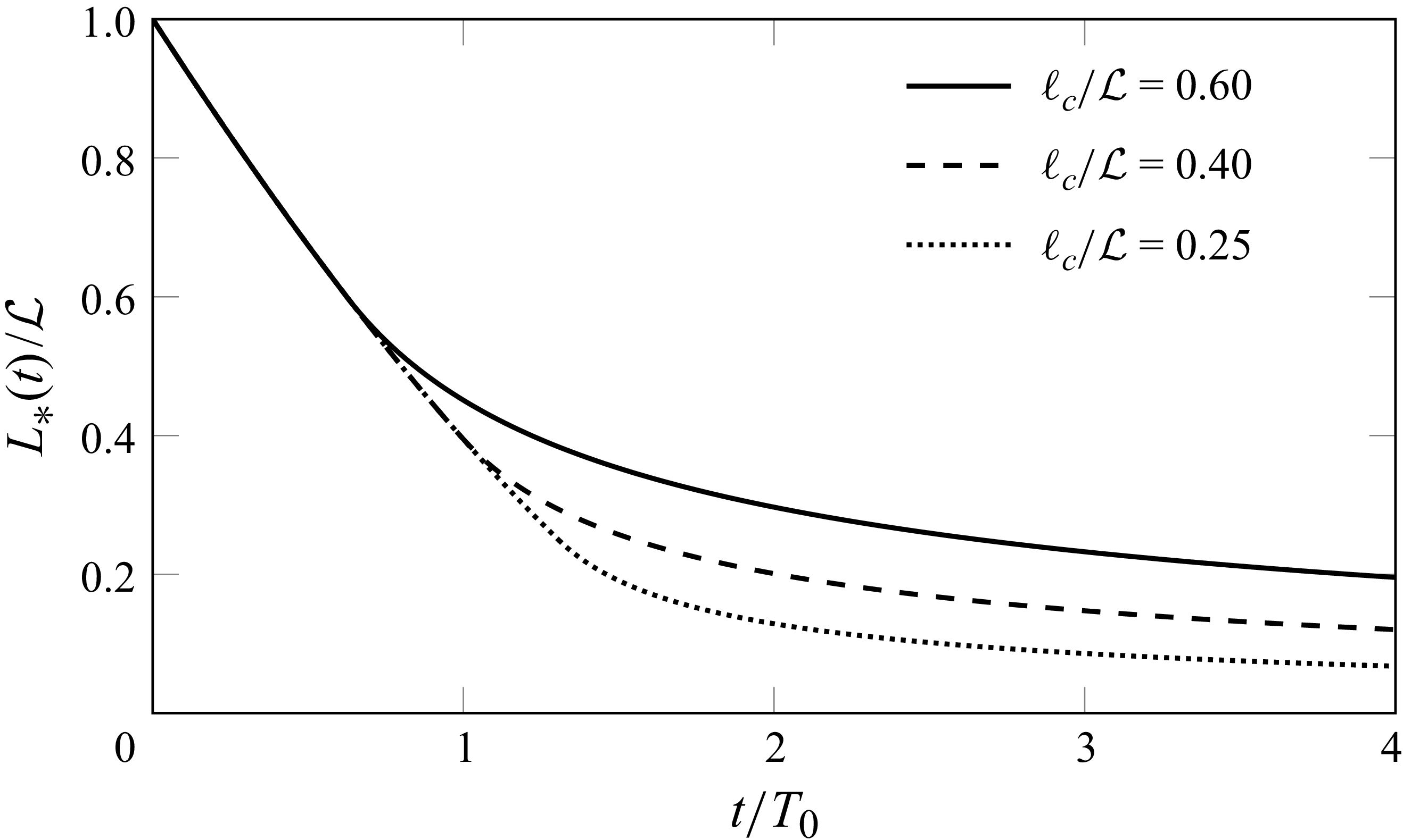


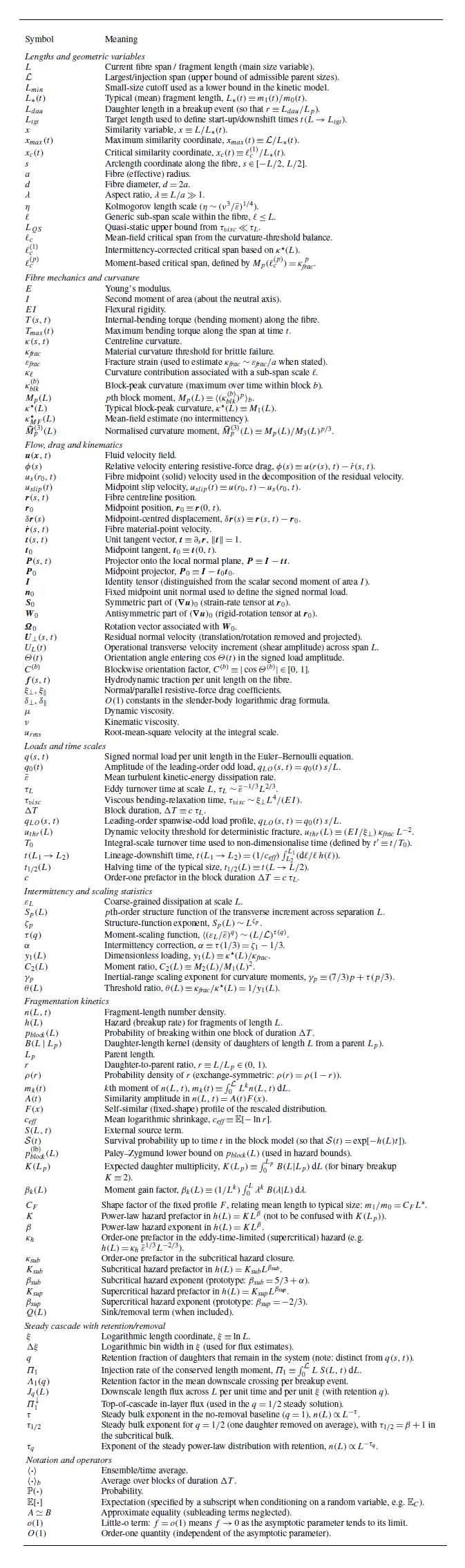


 Open access