





1. Introduction
The interaction between compressibility, surface roughness and heat transfer poses a longstanding challenge in the understanding and modelling of wall-bounded high-speed flows. These effects are central to many high-speed applications and directly impact drag and heat transfer, which are critical to the structural integrity of vehicles operating in and out of the atmosphere. In particular, the accurate prediction of thermal loads is inherently tied to our ability to assess the relation between velocity and temperature fields, which are nonlinearly coupled through density. However, surface roughness further complicates this coupling, and our predictive capabilities for such flows still rely heavily on semi-empirical correlations that do not generalise across the vast parameter space spanned by Mach number, wall-thermal conditions and roughness geometries (Bowersox Reference Bowersox2007).
In smooth-wall compressible boundary layers (BLs), mean thermodynamic quantities are related to the mean momentum field through the Reynolds analogy, independently formulated by Busemann (Reference Busemann1931) and Crocco (Reference Crocco1932) under the assumption of unit Prandtl number ( $ \textit{Pr}=1$
). Under this hypothesis, the mean temperature
$ \textit{Pr}=1$
). Under this hypothesis, the mean temperature $\bar {T}$
becomes a quadratic function of the mean streamwise velocity
$\bar {T}$
becomes a quadratic function of the mean streamwise velocity $\bar {u}$
, establishing a direct and remarkably simple connection between temperature and momentum fields.
$\bar {u}$
, establishing a direct and remarkably simple connection between temperature and momentum fields.
The assumption $ \textit{Pr}=1$
is central to the original derivation, as it implies identical molecular diffusivities of momentum and heat. However, real gases typically exhibit
$ \textit{Pr}=1$
is central to the original derivation, as it implies identical molecular diffusivities of momentum and heat. However, real gases typically exhibit $ \textit{Pr} \neq 1$
, and turbulent flows introduce an additional turbulent Prandtl number
$ \textit{Pr} \neq 1$
, and turbulent flows introduce an additional turbulent Prandtl number $ \textit{Pr}_t$
, reflecting the relative efficiency of turbulent momentum and heat transport. Deviations from unity, both at the molecular and turbulent levels, therefore, play a crucial role in determining the validity and accuracy of Reynolds-analogy-based relations.
$ \textit{Pr}_t$
, reflecting the relative efficiency of turbulent momentum and heat transport. Deviations from unity, both at the molecular and turbulent levels, therefore, play a crucial role in determining the validity and accuracy of Reynolds-analogy-based relations.
Subsequent studies introduced progressively refined corrections accounting for non-unity Prandtl number, wall heat transfer and more complex boundary conditions (Walz Reference Walz1969; Huang & Coleman Reference Huang and Coleman1994; Zhang et al. Reference Zhang, Bi, Hussain and She2014). These developments retained the quadratic temperature–velocity structure while modifying the coefficients to reflect realistic transport properties. A particularly systematic formulation is the generalised Reynolds analogy (GRA) proposed by Zhang et al. (Reference Zhang, Bi, Hussain and She2014). Rather than prescribing a specific recovery factor $r$
, the GRA introduces a generalised version,
$r$
, the GRA introduces a generalised version, $r_g$
, which incorporates Mach number and wall temperature effects.
$r_g$
, which incorporates Mach number and wall temperature effects.
The GRA has been assessed against an extensive set of direct numerical simulation (DNS) databases, including compressible channel flows, pipe flows and BLs with both adiabatic and cooled walls (Cogo et al. Reference Cogo, Baù, Chinappi, Bernardini and Picano2023), and has proven highly effective in rationalising smooth-wall compressible turbulence. Additionally, it serves as a general theoretical framework within which different modelling assumptions, including earlier formulations of Walz (Reference Walz1969) or Huang & Coleman (Reference Huang and Coleman1994), can be interpreted and systematically compared.
From an engineering standpoint, one of the most important observations of the extensive work dedicated to the Reynolds analogy is the universality of the Reynolds analogy factor $s=2C_h/C_{\kern-1.5pt f}$
, which is shown to hold approximately constant when coupled with the Prandtl number (
$s=2C_h/C_{\kern-1.5pt f}$
, which is shown to hold approximately constant when coupled with the Prandtl number ( $\textit{sPr}\approx 0.8)$
, with weak dependence on the Mach number and wall temperature condition (Zhang et al. Reference Zhang, Bi, Hussain and She2014; Cogo et al. Reference Cogo, Baù, Chinappi, Bernardini and Picano2023). Here,
$\textit{sPr}\approx 0.8)$
, with weak dependence on the Mach number and wall temperature condition (Zhang et al. Reference Zhang, Bi, Hussain and She2014; Cogo et al. Reference Cogo, Baù, Chinappi, Bernardini and Picano2023). Here, $C_{\kern-1.5pt f}=2\tau _w/(\rho _\infty u_\infty ^2)$
is the skin friction coefficient and
$C_{\kern-1.5pt f}=2\tau _w/(\rho _\infty u_\infty ^2)$
is the skin friction coefficient and $C_h=q_w/(\rho _{\infty }u_{\infty }c_{\kern-1pt p}(T_w-T_r))$
is the Stanton number, whose relation through
$C_h=q_w/(\rho _{\infty }u_{\infty }c_{\kern-1pt p}(T_w-T_r))$
is the Stanton number, whose relation through $s$
has far-reaching implications for reduced-order modelling, given that it directly relates the wall-shear stress
$s$
has far-reaching implications for reduced-order modelling, given that it directly relates the wall-shear stress $\tau _w$
and heat transfer
$\tau _w$
and heat transfer $q_w$
, where
$q_w$
, where $u_{\infty }$
is the freestream velocity,
$u_{\infty }$
is the freestream velocity, $\rho _{\infty }$
is the freestream density, and
$\rho _{\infty }$
is the freestream density, and $c_{\kern-1pt p}$
is the heat capacity at constant pressure.
$c_{\kern-1pt p}$
is the heat capacity at constant pressure.
In this context, it is well known that the presence of surface roughness clearly affects the value of $s$
(Hill, Voisinet & Wagner Reference Hill, Voisinet and Wagner1980; Modesti et al. Reference Modesti, Sathyanarayana, Salvadore and Bernardini2022), being usually lower than the reference smooth-wall case. The general consensus is that the increase in skin friction caused by roughness is greater than the corresponding increase in heat transfer. This is because the additional wall-shear stress is transmitted to the surface as a form drag on the individual asperities, while the heat flux is only controlled by the thermal conductivity (Owen & Thomson Reference Owen and Thomson1963). Several studies have been conducted to account for this effect with semi-empirical relations (Owen & Thomson Reference Owen and Thomson1963; Chen Reference Chen1972; Hill et al. Reference Hill, Voisinet and Wagner1980), which nevertheless suffer from poor generalisability.
$s$
(Hill, Voisinet & Wagner Reference Hill, Voisinet and Wagner1980; Modesti et al. Reference Modesti, Sathyanarayana, Salvadore and Bernardini2022), being usually lower than the reference smooth-wall case. The general consensus is that the increase in skin friction caused by roughness is greater than the corresponding increase in heat transfer. This is because the additional wall-shear stress is transmitted to the surface as a form drag on the individual asperities, while the heat flux is only controlled by the thermal conductivity (Owen & Thomson Reference Owen and Thomson1963). Several studies have been conducted to account for this effect with semi-empirical relations (Owen & Thomson Reference Owen and Thomson1963; Chen Reference Chen1972; Hill et al. Reference Hill, Voisinet and Wagner1980), which nevertheless suffer from poor generalisability.
Notwithstanding the additional layer of complexity added by rough surfaces, it is important to note that $s$
can be interpreted as an integral measure of the Reynolds analogy (RA) (Wenzel, Gibis & Kloker Reference Wenzel, Gibis and Kloker2022), and in this sense its departure from universality for rough-wall flows does not directly imply that the analogy between averaged momentum and energy equations is invalid locally everywhere in the flow.
$s$
can be interpreted as an integral measure of the Reynolds analogy (RA) (Wenzel, Gibis & Kloker Reference Wenzel, Gibis and Kloker2022), and in this sense its departure from universality for rough-wall flows does not directly imply that the analogy between averaged momentum and energy equations is invalid locally everywhere in the flow.
The present study aims to build on this consideration by assessing the validity of the RA throughout the entirety of the BL, which has important implications for the prediction of the wall heat transfer for compressible flows over rough walls. To this end, we leverage a novel DNS dataset of compressible turbulent BLs over prism-shaped roughness based on the works of Cogo et al. (Reference Cogo, Modesti, Bernardini and Picano2025a , Reference Cogo, Modesti, Picano and Bernardinib ), encompassing Mach numbers 2 and 4 and two wall temperature conditions: adiabatic and cold wall. Building on our findings, we propose a wall model for compressible rough-wall flows by extending the drag-predictive method introduced by Yang et al. (Reference Yang, Sadique, Mittal and Meneveau2016) for incompressible flows, which explicitly accounts for the sheltering mechanism induced by prism-shaped roughness.
2. Computational set-up
The present study is based on a novel dataset of DNSs of supersonic, zero-pressure-gradient, turbulent BL at free-stream Mach numbers of $M_\infty =2$
and
$M_\infty =2$
and $M_\infty =4$
, over cubical, aligned roughness elements. For each Mach number, we conduct one simulation at adiabatic conditions
$M_\infty =4$
, over cubical, aligned roughness elements. For each Mach number, we conduct one simulation at adiabatic conditions $\partial T/\partial y=0$
(or
$\partial T/\partial y=0$
(or $\varTheta = (T_w - T_\infty )/(T_r -T_\infty )\approx 1$
where
$\varTheta = (T_w - T_\infty )/(T_r -T_\infty )\approx 1$
where $T_r=T_\infty +r(\gamma -1)M_\infty ^2/2$
is the recovery temperature and
$T_r=T_\infty +r(\gamma -1)M_\infty ^2/2$
is the recovery temperature and $r= \textit{Pr}^{1/3}$
is the recovery factor), where
$r= \textit{Pr}^{1/3}$
is the recovery factor), where $\gamma$
is the speific heat ratio and cold wall isothermal conditions
$\gamma$
is the speific heat ratio and cold wall isothermal conditions $\varTheta = 0.25$
, for a total of four cases. In the present database, the use of the diabatic parameter
$\varTheta = 0.25$
, for a total of four cases. In the present database, the use of the diabatic parameter $\varTheta$
is adopted given its capability to recover the same behaviour in terms of wall cooling across different Mach numbers (Cogo et al. Reference Cogo, Baù, Chinappi, Bernardini and Picano2023).
$\varTheta$
is adopted given its capability to recover the same behaviour in terms of wall cooling across different Mach numbers (Cogo et al. Reference Cogo, Baù, Chinappi, Bernardini and Picano2023).
Throughout the manuscript, the four supersonic rough-wall boundary-layer cases are denoted as M2A, M2I, M4A and M4I, indicating the two Mach numbers considered and the wall-thermal condition, either adiabatic (A) or isothermal (I) (see table 2).
Schematic of the computational domain (not to scale), featuring an initial smooth surface followed by a rough region. The roughness pattern consists of three-dimensional wall-mounted cubical elements of height $k$
and spacing
$k$
and spacing $2k$
.
$2k$
.

Figure 1. Long description
A diagram of a computational domain representing a smooth-wall compressible BL followed by a rough region. The roughness pattern consists of three-dimensional wall-mounted cubical elements. The diagram includes labels for the dimensions of the domain and the spacing of the cubical elements. The flow direction is indicated by an arrow. The diagram is not to scale.
All rough cases in the present study feature the same roughness pattern, which is shared with the previous work of Cogo et al. (Reference Cogo, Modesti, Bernardini and Picano2025a
) and case CB_A of Cogo et al. (Reference Cogo, Modesti, Picano and Bernardini2025b
). This pattern consists of cubical elements of equal size $k$
equally spaced in the streamwise and spanwise directions by a length of
$k$
equally spaced in the streamwise and spanwise directions by a length of $2k$
. Compared with the inflow boundary-layer thickness
$2k$
. Compared with the inflow boundary-layer thickness $\delta _{\textit{in}}$
, the roughness height is
$\delta _{\textit{in}}$
, the roughness height is $k = 0.12\,\delta _{\textit{in}}$
. All DNS calculations are carried out using STREAmS (Bernardini et al. Reference Bernardini, Modesti, Salvadore, Sathyanarayana, Della Posta and Pirozzoli2023; Sathyanarayana et al. Reference Sathyanarayana, Bernardini, Modesti, Pirozzoli and Salvadore2025), an open source numerical solver orientated to modern high-performance-computing platforms using message-passing-interface parallelisation and supporting multi-GPU architectures. We solve the compressible Navier–Stokes equations for a viscous, heat-conducting gas, where molecular viscosity
$k = 0.12\,\delta _{\textit{in}}$
. All DNS calculations are carried out using STREAmS (Bernardini et al. Reference Bernardini, Modesti, Salvadore, Sathyanarayana, Della Posta and Pirozzoli2023; Sathyanarayana et al. Reference Sathyanarayana, Bernardini, Modesti, Pirozzoli and Salvadore2025), an open source numerical solver orientated to modern high-performance-computing platforms using message-passing-interface parallelisation and supporting multi-GPU architectures. We solve the compressible Navier–Stokes equations for a viscous, heat-conducting gas, where molecular viscosity $\mu$
is assumed to follow Sutherland’s law, with a reference free-stream temperature
$\mu$
is assumed to follow Sutherland’s law, with a reference free-stream temperature $T_\infty = 220 \ \text{K}$
. The thermal conductivity
$T_\infty = 220 \ \text{K}$
. The thermal conductivity $\lambda = \mu c_{\kern-1pt p}/ \textit{Pr}$
is related to the viscosity through the Prandtl number
$\lambda = \mu c_{\kern-1pt p}/ \textit{Pr}$
is related to the viscosity through the Prandtl number $ \textit{Pr} = 0.72$
. Convective terms are discretised using sixth-order, energy-preserving schemes in shock-free regions, while a high-order shock-capturing scheme weighted essentially non-oscillatory (WENO) is activated in the presence of shock waves, as identified by the Ducros sensor (Ducros et al. Reference Ducros, Ferrand, Nicoud, Weber, Darracq, Gacherieu and Poinsot1999). Viscous terms are discretised using a locally conservative formulation (De Vanna et al. Reference De Vanna, Benato, Picano and Benini2021) with sixth-order accuracy. The system of equations is completed by the equation of state for a calorically perfect gas and is solved on a Cartesian grid using a ghost-point-forcing immersed boundary method (IBM) to handle the complexity of the geometry. This method has been extensively validated for roughness in previous works by the same group (Cogo et al. Reference Cogo, Modesti, Bernardini and Picano2025a
,Reference Cogo, Modesti, Picano and Bernardini
b
). According to Chaudhuri et al. (Reference Chaudhuri, Hadjadj and Chinnayya2011), when combined with shock-capturing schemes and a fifth-order WENO discretisation, the IBM exhibits second-order accuracy in the vicinity of solid boundaries. The computational domain consists of a smooth-wall inflow region used to generate a fully turbulent BL of initial thickness
$ \textit{Pr} = 0.72$
. Convective terms are discretised using sixth-order, energy-preserving schemes in shock-free regions, while a high-order shock-capturing scheme weighted essentially non-oscillatory (WENO) is activated in the presence of shock waves, as identified by the Ducros sensor (Ducros et al. Reference Ducros, Ferrand, Nicoud, Weber, Darracq, Gacherieu and Poinsot1999). Viscous terms are discretised using a locally conservative formulation (De Vanna et al. Reference De Vanna, Benato, Picano and Benini2021) with sixth-order accuracy. The system of equations is completed by the equation of state for a calorically perfect gas and is solved on a Cartesian grid using a ghost-point-forcing immersed boundary method (IBM) to handle the complexity of the geometry. This method has been extensively validated for roughness in previous works by the same group (Cogo et al. Reference Cogo, Modesti, Bernardini and Picano2025a
,Reference Cogo, Modesti, Picano and Bernardini
b
). According to Chaudhuri et al. (Reference Chaudhuri, Hadjadj and Chinnayya2011), when combined with shock-capturing schemes and a fifth-order WENO discretisation, the IBM exhibits second-order accuracy in the vicinity of solid boundaries. The computational domain consists of a smooth-wall inflow region used to generate a fully turbulent BL of initial thickness $\delta _{\textit{in}}$
via a recycling–rescaling procedure, followed downstream by a rough-wall region starting from
$\delta _{\textit{in}}$
via a recycling–rescaling procedure, followed downstream by a rough-wall region starting from $x = 55\,\delta _{\mathit{in}}$
, where prism-shaped roughness elements are embedded, see figure 1. The domain extends
$x = 55\,\delta _{\mathit{in}}$
, where prism-shaped roughness elements are embedded, see figure 1. The domain extends $L_x \times L_y \times L_z = 150 \times 25 \times 8.28\, \delta _{\textit{in}}$
, with the recycling plane at
$L_x \times L_y \times L_z = 150 \times 25 \times 8.28\, \delta _{\textit{in}}$
, with the recycling plane at $x = 40\,\delta _{\textit{in}}$
, the rough region spanning
$x = 40\,\delta _{\textit{in}}$
, the rough region spanning $55 \leqslant x/\delta _{\textit{in}} \leqslant 147$
and a short smooth-wall buffer before the outflow. Non-reflecting boundary conditions based on characteristic decomposition are imposed at the upper and outflow boundaries. The spanwise boundary condition is periodic and implemented with the same formal accuracy as the interior scheme. The spanwise domain accommodates 23 repetitive roughness units (each of width
$55 \leqslant x/\delta _{\textit{in}} \leqslant 147$
and a short smooth-wall buffer before the outflow. Non-reflecting boundary conditions based on characteristic decomposition are imposed at the upper and outflow boundaries. The spanwise boundary condition is periodic and implemented with the same formal accuracy as the interior scheme. The spanwise domain accommodates 23 repetitive roughness units (each of width $3k$
), ensuring that the periodic boundary condition does not artificially constrain the turbulent structures in the spanwise direction and that statistical homogeneity is well preserved.
$3k$
), ensuring that the periodic boundary condition does not artificially constrain the turbulent structures in the spanwise direction and that statistical homogeneity is well preserved.
All simulations share the same grid resolution, composed of $20240 \times 556 \times 1408$
points in the streamwise, wall-normal and spanwise directions, respectively. The spanwise grid spacing is uniform throughout the domain. In the streamwise direction, a coarser spacing is used in the smooth inflow region and gradually refined towards the rough-wall region, with a streamwise refinement ratio of
$20240 \times 556 \times 1408$
points in the streamwise, wall-normal and spanwise directions, respectively. The spanwise grid spacing is uniform throughout the domain. In the streamwise direction, a coarser spacing is used in the smooth inflow region and gradually refined towards the rough-wall region, with a streamwise refinement ratio of $2.5$
. In the wall-normal direction, approximately 40 grid points are distributed within the roughness height
$2.5$
. In the wall-normal direction, approximately 40 grid points are distributed within the roughness height $k$
, with nearly uniform spacing up to the roughness crest; the mesh is then progressively coarsened through the BL up to
$k$
, with nearly uniform spacing up to the roughness crest; the mesh is then progressively coarsened through the BL up to $y \approx 3.8\,\delta _{\textit{in}}$
(local stretching ratio
$y \approx 3.8\,\delta _{\textit{in}}$
(local stretching ratio $\approx 8$
), beyond which a stronger stretching (local ratio
$\approx 8$
), beyond which a stronger stretching (local ratio $\approx 20$
) is applied up to the top of the domain.
$\approx 20$
) is applied up to the top of the domain.
The local grid resolution in wall units at representative smooth- and rough-wall streamwise stations is reported in table 1, together with key boundary-layer properties. From this table it is evident that the resolution requirements imposed by the need to accurately resolve the roughness elements are more demanding than those dictated by the turbulent flow alone, and that the present simulations are well within DNS quality standards for all cases.
Grid resolution and boundary-layer properties at selected smooth and rough streamwise stations for each DNS case. Here, $\Delta x^+$
and
$\Delta x^+$
and $\Delta z^+$
are the streamwise and spanwise grid spacings in wall units,
$\Delta z^+$
are the streamwise and spanwise grid spacings in wall units, $\Delta y_w^+$
is the wall-normal spacing at the bottom wall,
$\Delta y_w^+$
is the wall-normal spacing at the bottom wall, $\Delta y_k^+$
at the roughness crest and
$\Delta y_k^+$
at the roughness crest and $\Delta y_\delta ^+$
at the boundary-layer edge. Here,
$\Delta y_\delta ^+$
at the boundary-layer edge. Here, $Re_\theta =\rho _\infty u_\infty \theta / \mu _\infty$
, where
$Re_\theta =\rho _\infty u_\infty \theta / \mu _\infty$
, where $\theta$
is the momentum thickness.
$\theta$
is the momentum thickness.

Table 1. Long description
The table presents data on grid resolution and boundary-layer properties at selected smooth and rough streamwise stations for each DNS case. It includes four rows and eight columns. The columns are labeled as Case, Station, Δx+, Δz+, Δy+_w, Δy+_k, Δy+_δ, δ_99/δ_in, Re_τ, and Re_θ. The rows are labeled with specific cases and stations. Each row provides values for the streamwise and spanwise grid spacings in wall units, wall-normal spacing at different levels, and Reynolds numbers. For example, Row 1: Case M2A, Station x/δ_in = 50, Δx+ = 2.6, Δz+ = 2.3, Δy+_w = 0.4, Δy+_k = —, Δy+_δ = 5.1, δ_99/δ_in = 1.8, Re_τ = 694, Re_θ = 3314.
Summary of parameters for DNS study at selected station, $x=127 \delta _{\textit{in}}$
. Here,
$x=127 \delta _{\textit{in}}$
. Here,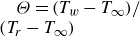 $\varTheta =(T_w-T_\infty )/(T_r-T_\infty )$
is the diabatic parameter,
$\varTheta =(T_w-T_\infty )/(T_r-T_\infty )$
is the diabatic parameter, $T_w/T_r$
the wall-to-recovery temperature ratio,
$T_w/T_r$
the wall-to-recovery temperature ratio, $Re_\tau =\rho _wu_\tau \delta _{99}/\mu _w$
the friction Reynolds number,
$Re_\tau =\rho _wu_\tau \delta _{99}/\mu _w$
the friction Reynolds number, $k$
the roughness height and
$k$
the roughness height and $\bar {M}_k$
the averaged Mach number at the roughness crest. The boundary-layer thickness
$\bar {M}_k$
the averaged Mach number at the roughness crest. The boundary-layer thickness $\delta _{99}$
is computed using the location where
$\delta _{99}$
is computed using the location where $\bar {u}/u_\infty =0.99$
.
$\bar {u}/u_\infty =0.99$
.

Table 2. Long description
A table comparing parameters for different supersonic rough-wall boundary-layer cases. The table has six columns and five rows, including a header row. The columns are labeled Colour, Case, M infinity, M tilde k, Surface, Theta, T w over T r, R e tau, delta 99 over k, and k plus. The rows provide data for cases M 03, M 2 A, M 2 I, M 4 A, and M 4 I. Each row lists specific values for the parameters. For example, the first row for case M 03 shows values like 0.3 for M infinity, Cubical for Surface, 1.0 for Theta, 1.0 for T w over T r, 1600 for R e tau, 28.5 for delta 99 over k, and 56 for k plus. The table provides a detailed comparison of these parameters across different cases.
Reynolds averages are computed by combining averaging in the spanwise direction, temporal averaging over at least $500\,\delta _{\mathit{in}}/u_\infty$
and averaging over a short streamwise window of four roughness wavelengths. Below the roughness crest, an intrinsic (fluid-only) spatial average is applied. Resources for one simulation consisted of 64 nodes with 4 x GPUs/node (256 GPUs in total) for a domain discretised with approximately 16 billion nodes and it was computed by the Leonardo cluster at CINECA. All four cases have been sampled at the streamwise station
$500\,\delta _{\mathit{in}}/u_\infty$
and averaging over a short streamwise window of four roughness wavelengths. Below the roughness crest, an intrinsic (fluid-only) spatial average is applied. Resources for one simulation consisted of 64 nodes with 4 x GPUs/node (256 GPUs in total) for a domain discretised with approximately 16 billion nodes and it was computed by the Leonardo cluster at CINECA. All four cases have been sampled at the streamwise station $x/\delta _{\mathit{in}} = 127$
, ensuring an acceptable adjustment of the flow to the rough surface after the smooth-to-rough transition, and related properties are reported in table 2, including the friction Reynolds number
$x/\delta _{\mathit{in}} = 127$
, ensuring an acceptable adjustment of the flow to the rough surface after the smooth-to-rough transition, and related properties are reported in table 2, including the friction Reynolds number $Re_\tau$
, the ratio
$Re_\tau$
, the ratio $k/\delta _{99}$
and the roughness Reynolds number
$k/\delta _{99}$
and the roughness Reynolds number $k^+$
.
$k^+$
.
3. Database overview
3.1. Instantaneous and mean flow fields
To provide a qualitative overview of the interaction between the mean flow dynamics and the roughness elements, figure 2 shows portions of streamwise- wall-normal $x$
–
$x$
– $y$
planes coloured by the instantaneous temperature, whose variability clearly reflects Mach number effects (increasing from top to bottom) and diabatic parameter (increasing from left to right). The influence of the Mach number is evident across all cases with an increase in the maximum temperature near the wall, especially in adiabatic cases (right column). However, strong wall cooling (left column) attenuates this effect, as the flow is required to equilibrate with a wall temperature that is considerably lower than the adiabatic wall temperature. These observations are in qualitative agreement with the general trends found in smooth-wall flows at the same
$y$
planes coloured by the instantaneous temperature, whose variability clearly reflects Mach number effects (increasing from top to bottom) and diabatic parameter (increasing from left to right). The influence of the Mach number is evident across all cases with an increase in the maximum temperature near the wall, especially in adiabatic cases (right column). However, strong wall cooling (left column) attenuates this effect, as the flow is required to equilibrate with a wall temperature that is considerably lower than the adiabatic wall temperature. These observations are in qualitative agreement with the general trends found in smooth-wall flows at the same $M_\infty$
and
$M_\infty$
and $\varTheta$
(Cogo et al. Reference Cogo, Baù, Chinappi, Bernardini and Picano2023), and are inherently tied to the distribution of wall-normal temperature, reflecting both Mach number (higher
$\varTheta$
(Cogo et al. Reference Cogo, Baù, Chinappi, Bernardini and Picano2023), and are inherently tied to the distribution of wall-normal temperature, reflecting both Mach number (higher $T_{aw}$
with increasing
$T_{aw}$
with increasing $M_\infty$
) and wall cooling effects (
$M_\infty$
) and wall cooling effects ( $T_w\lt T_{aw}$
as
$T_w\lt T_{aw}$
as $\varTheta \lt 1$
).
$\varTheta \lt 1$
).
Instantaneous temperature field $T/T_\infty$
visualised in an
$T/T_\infty$
visualised in an $x$
–
$x$
– $y$
slice bisecting half the roughness elements. Panels show cases (a) M2I, (b) M2A, (c) M4I, (d) M4A. The white dashed line denotes the average location of the boundary-layer thickness
$y$
slice bisecting half the roughness elements. Panels show cases (a) M2I, (b) M2A, (c) M4I, (d) M4A. The white dashed line denotes the average location of the boundary-layer thickness $\delta _{99}$
.
$\delta _{99}$
.

Numerical schlieren $\textit{exp}(-100|\boldsymbol{\nabla }\bar {\rho }|)$
obtained from the averaged density field
$\textit{exp}(-100|\boldsymbol{\nabla }\bar {\rho }|)$
obtained from the averaged density field $\bar {\rho }/\rho _\infty$
visualised in an
$\bar {\rho }/\rho _\infty$
visualised in an $x$
–
$x$
– $y$
slice. Values range from
$y$
slice. Values range from $0.5$
to
$0.5$
to $1.1$
. In dashed red: sonic line representative of unity local Mach number. White dashed lines represent the boundary-layer thickness
$1.1$
. In dashed red: sonic line representative of unity local Mach number. White dashed lines represent the boundary-layer thickness $\delta _{99}$
. (Inset) Contour of averaged Mach number with values ranging from 0 (red) to 1 (blue). (a) M2I, (b) M2A, (c) M4I, (d) M4A.
$\delta _{99}$
. (Inset) Contour of averaged Mach number with values ranging from 0 (red) to 1 (blue). (a) M2I, (b) M2A, (c) M4I, (d) M4A.

Figure 3. Long description
Panel A: A numerical schlieren image showing the density field in a slice. The x-axis is labeled x/delta_in and the y-axis is labeled y/delta_in. The dashed red line represents the sonic line at a local Mach number of unity. The white dashed lines indicate the boundary-layer thickness. The inset shows a contour of the averaged Mach number, with values ranging from 0 (red) to 1 (blue). Panel B: Similar to Panel A, this numerical schlieren image also shows the density field with the same labels and lines. The inset again displays the contour of the averaged Mach number. Panel C: Another numerical schlieren image depicting the density field with identical labels and lines. The inset shows the contour of the averaged Mach number. Panel D: The final numerical schlieren image in the series, with the same labels and lines. The inset shows the contour of the averaged Mach number.
The mean dynamics of the near-wall region is reported as numerical schlieren in figure 3, where we consider both time and spanwise averages. Several important features emerge from this figure. First, the overall darkness of the visualisation varies systematically with wall-thermal conditions: figure 3(a) for case M2I appears notably darker than its adiabatic counterpart, figure 3(b), and similarly for figures 3(c) and 3(d) at Mach 4. This reflects the more uniform temperature distribution in isothermal cases noted for figure 2.
The red dashed contour line in figure 3 delineates the sonic line, where the local flow velocity magnitude equals the local speed of sound $\bar {a}=\sqrt {\gamma R \bar {T}}$
, where
$\bar {a}=\sqrt {\gamma R \bar {T}}$
, where $R$
is a specific gas constant, corresponding to unit local Mach number. This contour effectively separates the supersonic outer region from the subsonic near-wall layer. As expected, in the Mach 4 cases the sonic line is located considerably closer to the wall than in Mach 2, indicating that a larger fraction of the BL operates in supersonic conditions. Furthermore, within each Mach number pair, the isothermal-wall cases exhibit sonic lines positioned even closer to the surface. This reflects the reduced near-wall temperature in cooled-wall configurations, which lowers the local speed of sound and causes the sonic condition to be reached at smaller wall-normal distances.
$R$
is a specific gas constant, corresponding to unit local Mach number. This contour effectively separates the supersonic outer region from the subsonic near-wall layer. As expected, in the Mach 4 cases the sonic line is located considerably closer to the wall than in Mach 2, indicating that a larger fraction of the BL operates in supersonic conditions. Furthermore, within each Mach number pair, the isothermal-wall cases exhibit sonic lines positioned even closer to the surface. This reflects the reduced near-wall temperature in cooled-wall configurations, which lowers the local speed of sound and causes the sonic condition to be reached at smaller wall-normal distances.
An important observation is that, at the selected measurement station and for both Mach numbers, the roughness elements do not generate discernible shock waves that would introduce large discontinuities in the mean flow. This suggests that the roughness height remains sufficiently submerged within the subsonic layer. This behaviour is also evident in the insets of figure 3, which display the average local Mach number. As reported in table 2, the Mach number at the roughness crest, $\bar {M}_k$
, remains below unity, and the ratios between the height of the sonic line and the roughness crest are:
$\bar {M}_k$
, remains below unity, and the ratios between the height of the sonic line and the roughness crest are: $5.35$
for M2I,
$5.35$
for M2I, $5.95$
for M2A,
$5.95$
for M2A, $1.88$
for M4I and
$1.88$
for M4I and $2.08$
for M4A. Nevertheless, we do not exclude that at different flow conditions or for more complex roughness configurations, the elements could protrude into the local supersonic region for a portion of their height, potentially generating shock structures, as observed by Peltier, Humble & Bowersox (Reference Peltier, Humble and Bowersox2016).
$2.08$
for M4A. Nevertheless, we do not exclude that at different flow conditions or for more complex roughness configurations, the elements could protrude into the local supersonic region for a portion of their height, potentially generating shock structures, as observed by Peltier, Humble & Bowersox (Reference Peltier, Humble and Bowersox2016).
Finally, the insets in figure 3, representative of the average local Mach number, show a distinct region of low-momentum fluid in the immediate wake of each roughness element. The spatial extent of this sheltered region, characterised by reduced velocity and elevated temperature relative to the undisturbed flow at the same wall-normal location, plays a crucial role in determining the associated form drag (Cogo et al. Reference Cogo, Modesti, Picano and Bernardini2025b ). This sheltering mechanism has been systematically modelled by Yang et al. (Reference Yang, Sadique, Mittal and Meneveau2016) for incompressible flows over prism-shaped roughness and will be considered in this study in § 6.
3.2. Streamwise evolution of wall statistics
Figure 4 presents the streamwise evolution of key integral quantities following the smooth-to-rough transition at $x/\delta _{\mathit{in}} = 55$
; the periodic oscillations visible in the rough-wall region reflect the streamwise-periodic modulation imprinted by the roughness array, spaced at multiples of the roughness wavelength
$x/\delta _{\mathit{in}} = 55$
; the periodic oscillations visible in the rough-wall region reflect the streamwise-periodic modulation imprinted by the roughness array, spaced at multiples of the roughness wavelength $\lambda$
.
$\lambda$
.
Mean streamwise profiles of (a) skin friction coefficient $C_{\kern-1.5pt f}=\tau _w/(1/2\rho _\infty u_\infty ^2)$
, (b) Stanton number
$C_{\kern-1.5pt f}=\tau _w/(1/2\rho _\infty u_\infty ^2)$
, (b) Stanton number $C_h=q_w/(\rho _\infty u_\infty c_{\kern-1pt p}(T_w-T_r))$
, (c) RA factor
$C_h=q_w/(\rho _\infty u_\infty c_{\kern-1pt p}(T_w-T_r))$
, (c) RA factor $s Pr = 2 C_h/ C_{\kern-1.5pt f} Pr$
.
$s Pr = 2 C_h/ C_{\kern-1.5pt f} Pr$
.

Figure 4(a) shows the skin friction coefficient $C_{\kern-1.5pt f}$
for all four configurations. A sharp peak occurs immediately downstream of the transition, followed by a gradual relaxation as the flow adjusts to the new wall condition, consistent with previous studies (Rouhi, Chung & Hutchins Reference Rouhi, Chung and Hutchins2019; Cogo et al. Reference Cogo, Modesti, Picano and Bernardini2025b
). The influence of Mach number and wall temperature in the rough region follows the same trends as the smooth-wall counterpart (Huang, Duan & Choudhari Reference Huang, Duan and Choudhari2022; Cogo et al. Reference Cogo, Baù, Chinappi, Bernardini and Picano2023):
$C_{\kern-1.5pt f}$
for all four configurations. A sharp peak occurs immediately downstream of the transition, followed by a gradual relaxation as the flow adjusts to the new wall condition, consistent with previous studies (Rouhi, Chung & Hutchins Reference Rouhi, Chung and Hutchins2019; Cogo et al. Reference Cogo, Modesti, Picano and Bernardini2025b
). The influence of Mach number and wall temperature in the rough region follows the same trends as the smooth-wall counterpart (Huang, Duan & Choudhari Reference Huang, Duan and Choudhari2022; Cogo et al. Reference Cogo, Baù, Chinappi, Bernardini and Picano2023): $C_{\kern-1.5pt f}$
decreases with increasing Mach number and increases with wall cooling (
$C_{\kern-1.5pt f}$
decreases with increasing Mach number and increases with wall cooling ( $T_w\lt T_{aw}$
).
$T_w\lt T_{aw}$
).
Figure 4(b) shows the Stanton number $C_h$
for the isothermal cases (M2I, M4I), which exhibits qualitatively similar behaviour to
$C_h$
for the isothermal cases (M2I, M4I), which exhibits qualitatively similar behaviour to $C_{\kern-1.5pt f}$
. The case M2I consistently shows higher heat transfer than M4I in both smooth and rough regions. Both cases show a gradual decay downstream of the transition, with M2I maintaining approximately twice the heat transfer rate of M4I throughout the domain.
$C_{\kern-1.5pt f}$
. The case M2I consistently shows higher heat transfer than M4I in both smooth and rough regions. Both cases show a gradual decay downstream of the transition, with M2I maintaining approximately twice the heat transfer rate of M4I throughout the domain.
Figure 4(c) presents the RA factor multiplied by the Prandtl number, $ \textit{sPr}$
, where
$ \textit{sPr}$
, where $s = 2C_h/C_{\kern-1.5pt f}$
. This is a classical integral measure of the RA that has been extensively studied in smooth-wall flows (Zhang et al. Reference Zhang, Bi, Hussain and She2014; Wenzel et al. Reference Wenzel, Gibis and Kloker2022; Cogo et al. Reference Cogo, Baù, Chinappi, Bernardini and Picano2023). These studies showed that smooth-wall compressible flows exhibit excellent universality, with
$s = 2C_h/C_{\kern-1.5pt f}$
. This is a classical integral measure of the RA that has been extensively studied in smooth-wall flows (Zhang et al. Reference Zhang, Bi, Hussain and She2014; Wenzel et al. Reference Wenzel, Gibis and Kloker2022; Cogo et al. Reference Cogo, Baù, Chinappi, Bernardini and Picano2023). These studies showed that smooth-wall compressible flows exhibit excellent universality, with $\textit{sPr} = 0.8 \pm 0.03$
(Cogo et al. Reference Cogo, Baù, Chinappi, Bernardini and Picano2023) regardless of Mach number, wall temperature or Reynolds number. This value is clearly observed here for both M2I and M4I in the smooth region before the onset of roughness. After the smooth-to-rough transition, both cases show a dramatic drop to
$\textit{sPr} = 0.8 \pm 0.03$
(Cogo et al. Reference Cogo, Baù, Chinappi, Bernardini and Picano2023) regardless of Mach number, wall temperature or Reynolds number. This value is clearly observed here for both M2I and M4I in the smooth region before the onset of roughness. After the smooth-to-rough transition, both cases show a dramatic drop to $ \textit{sPr} \approx 0.4$
–
$ \textit{sPr} \approx 0.4$
– $0.5$
at the transition, followed by gradual relaxation that does not recover the smooth-wall reference value. More importantly, M4I exhibits a distinctly lower
$0.5$
at the transition, followed by gradual relaxation that does not recover the smooth-wall reference value. More importantly, M4I exhibits a distinctly lower $ \textit{sPr}$
than M2I, undermining its universality among rough-wall cases.
$ \textit{sPr}$
than M2I, undermining its universality among rough-wall cases.
This behaviour is well documented not only in high-speed flows but also in incompressible wall-bounded flows with heat transfer (Bons Reference Bons2005), where $ \textit{sPr}$
varies significantly depending on the roughness geometry. This fact reflects the fundamental differences between momentum transport (dominated by form drag on roughness elements) and heat transfer (governed by thermal conduction) in the roughness sublayer, which prevent the use of an integral indicator for the RA (Owen & Thomson Reference Owen and Thomson1963). Despite this, § 4 demonstrates that a local formulation of the RA for the mean flow can still be applied outside the direct influence of roughness. We address this by examining a wall-normal location far from the roughness transition, at
$ \textit{sPr}$
varies significantly depending on the roughness geometry. This fact reflects the fundamental differences between momentum transport (dominated by form drag on roughness elements) and heat transfer (governed by thermal conduction) in the roughness sublayer, which prevent the use of an integral indicator for the RA (Owen & Thomson Reference Owen and Thomson1963). Despite this, § 4 demonstrates that a local formulation of the RA for the mean flow can still be applied outside the direct influence of roughness. We address this by examining a wall-normal location far from the roughness transition, at $x/\delta _{\mathit{in}} = 127$
, where all cases appear reasonably equilibrated.
$x/\delta _{\mathit{in}} = 127$
, where all cases appear reasonably equilibrated.
4. Validity of the Reynolds analogy
4.1. Framework of the Reynolds analogy for mean flows
The formulation of the RA for mean flows, generalised by Zhang et al. (Reference Zhang, Bi, Hussain and She2014), establishes a direct relation between the mean velocity $\bar {u}$
and the defect of a generalised recovery enthalpy,
$\bar {u}$
and the defect of a generalised recovery enthalpy, $\bar {H}_g-\bar {H}_w$
, namely
$\bar {H}_g-\bar {H}_w$
, namely
 \begin{align} \bar {H}_g-\bar {H}_w = U_w \bar {u}, \end{align}
where $H_g=c_{\kern-1pt p}T+r_g u^2/2$
is a generalised recovery enthalpy defined in terms of the recovery factor
$H_g=c_{\kern-1pt p}T+r_g u^2/2$
is a generalised recovery enthalpy defined in terms of the recovery factor $r_g$
.
$r_g$
.
Equation (4.1) implies that the proportionality between the mean enthalpy and velocity fields is governed by a constant velocity scale $U_w$
. Rewriting (4.1) in terms of temperature yields a quadratic relation between the mean temperature and velocity
$U_w$
. Rewriting (4.1) in terms of temperature yields a quadratic relation between the mean temperature and velocity
 \begin{align} \bar {T}=T_w+\frac {U_w}{c_{\kern-1pt p}}\bar {u}-\frac {r_g}{2c_{\kern-1pt p}}\bar {u}^2, \end{align}
which satisfies the wall boundary condition $\bar {T}=T_w$
when
$\bar {T}=T_w$
when $\bar {u}=0$
. In this formulation, the coefficients
$\bar {u}=0$
. In this formulation, the coefficients $U_w$
and
$U_w$
and $r_g$
determine the linear and quadratic contributions of the velocity field to the temperature distribution.
$r_g$
determine the linear and quadratic contributions of the velocity field to the temperature distribution.
Equation (4.2) provides a convenient framework to interpret several classical temperature–velocity relations proposed in the literature, which can be viewed as particular closures for the coefficients $U_w$
and
$U_w$
and $r_g$
depending on the assumed coupling between momentum and heat transfer.
$r_g$
depending on the assumed coupling between momentum and heat transfer.
4.2. Classical formulations
The earliest form of this relation can be traced back to the Crocco–Busemann theory (Crocco Reference Crocco1932), derived for compressible BLs under the assumptions of constant properties and unit Prandtl number. Under these conditions the quadratic coefficient reduces to $r_g=1$
, while the linear coefficient depends on the difference between wall and stagnation temperatures, leading to a temperature–velocity relation based on the stagnation temperature
$r_g=1$
, while the linear coefficient depends on the difference between wall and stagnation temperatures, leading to a temperature–velocity relation based on the stagnation temperature $T_0$
.
$T_0$
.
For turbulent BLs, Walz (Reference Walz1969) introduced the concept of recovery temperature $T_r$
to account for the departure from unity of the Prandtl number. This modification introduces a recovery factor
$T_r$
to account for the departure from unity of the Prandtl number. This modification introduces a recovery factor $r$
, typically approximated as
$r$
, typically approximated as $r\approx \textit{Pr}^{1/3}$
, which replaces the unit coefficient of the Crocco formulation and yields the well-known Walz relation.
$r\approx \textit{Pr}^{1/3}$
, which replaces the unit coefficient of the Crocco formulation and yields the well-known Walz relation.
Alternative formulations express the temperature–velocity relation directly in terms of wall fluxes. In particular, the model proposed by Huang & Coleman (Reference Huang and Coleman1994) relates the linear coefficient to the ratio between wall heat flux and wall-shear stress, $q_w/\tau _w$
, together with an effective Prandtl number
$q_w/\tau _w$
, together with an effective Prandtl number $ \textit{Pr}_e$
representing a combination of molecular and turbulent transport effects, whose best fit from DNSs has been reported as
$ \textit{Pr}_e$
representing a combination of molecular and turbulent transport effects, whose best fit from DNSs has been reported as $ \textit{Pr}_e\approx 0.8$
(Larsson & Pirozzoli Reference Larsson and Pirozzoli2026). This approach is convenient when wall fluxes are known or can be estimated.
$ \textit{Pr}_e\approx 0.8$
(Larsson & Pirozzoli Reference Larsson and Pirozzoli2026). This approach is convenient when wall fluxes are known or can be estimated.
More recently, Zhang et al. (Reference Zhang, Bi, Hussain and She2014) proposed a generalised recovery factor $r_g$
that depends explicitly on both the wall heat flux and the external flow conditions. In this formulation, the coefficients of (4.2) are obtained by simultaneously enforcing the outer boundary condition and the relation between wall heat and momentum fluxes, providing a unified framework that recovers the Crocco and Walz analogies as limiting cases for
$r_g$
that depends explicitly on both the wall heat flux and the external flow conditions. In this formulation, the coefficients of (4.2) are obtained by simultaneously enforcing the outer boundary condition and the relation between wall heat and momentum fluxes, providing a unified framework that recovers the Crocco and Walz analogies as limiting cases for $ \textit{Pr}=1$
and adiabatic conditions.
$ \textit{Pr}=1$
and adiabatic conditions.
The formulations described above can be systematically characterised by the degree of freedom they assign to the coefficients of (4.2). The Crocco–Busemann and Walz relations prescribe both $r_g$
and the functional form of
$r_g$
and the functional form of $U_w$
, leaving no free parameters once the outer boundary condition is imposed. The Huang & Coleman (Reference Huang and Coleman1994) relation similarly fixes
$U_w$
, leaving no free parameters once the outer boundary condition is imposed. The Huang & Coleman (Reference Huang and Coleman1994) relation similarly fixes $r_g= \textit{Pr}_e$
, expressing
$r_g= \textit{Pr}_e$
, expressing $U_w$
through the wall-flux ratio
$U_w$
through the wall-flux ratio $q_w/\tau _w$
. In contrast, the GRA of Zhang et al. (Reference Zhang, Bi, Hussain and She2014) leaves
$q_w/\tau _w$
. In contrast, the GRA of Zhang et al. (Reference Zhang, Bi, Hussain and She2014) leaves $r_g$
as a free parameter, determining it self-consistently by simultaneously enforcing the outer boundary condition and the wall-flux relation. A summary of these formulations and their corresponding coefficients is reported in table 3.
$r_g$
as a free parameter, determining it self-consistently by simultaneously enforcing the outer boundary condition and the wall-flux relation. A summary of these formulations and their corresponding coefficients is reported in table 3.
Original formulation of the RA for the mean temperature–velocity relation with various approaches. In smooth-wall flows, the formulations that rely on the unknown ratio $q_w/\tau _w$
can be closed by invoking the universality of the RA factor
$q_w/\tau _w$
can be closed by invoking the universality of the RA factor $s Pr=2 C_h/C_{\kern-1.5pt f} Pr \approx 0.8$
.
$s Pr=2 C_h/C_{\kern-1.5pt f} Pr \approx 0.8$
.

Table 3. Long description
A table comparing different approaches to temperature recovery in fluid dynamics. The table has five rows and four columns. The columns are labeled Approach, Equation, Total temperature, and Recovery factor. The rows are labeled General, Crocco (1932), Walz (1969), Huang & Coleman (1994), and Zhang et al. (2014). Row 1: Approach, General; Equation, T-tilde = T-w + c1 u-tilde - c2 u-tilde squared; Total temperature, blank; Recovery factor, blank. Row 2: Approach, Crocco (1932); Equation, T-tilde = T-w + (T0 - T-w)/u-beta * u-tilde - 1/(2 c-p) * u-tilde squared; Total temperature, T0 = T-beta + u-beta squared / (2 c-p); Recovery factor, blank. Row 3: Approach, Walz (1969); Equation, T-tilde = T-w + (T-r - T-w)/u-beta * u-tilde - r / (2 c-p) * u-tilde squared; Total temperature, T-r = T-beta + r * u-beta squared / (2 c-p); Recovery factor, r = P-r * P-r to the power 1/3. Row 4: Approach, Huang & Coleman (1994); Equation, T-tilde = T-w - (P-r * q-w) / (c-p * T-w) * u-tilde - P-r-e / (2 c-p) * u-tilde squared; Total temperature, blank; Recovery factor, P-r-e is approximately equal to 0.8. Row 5: Approach, Zhang et al. (2014); Equation, T-tilde = T-w + (T-r-g - T-w)/u-beta * u-tilde - r-g / (2 c-p) * u-tilde squared; Total temperature, T-r-g = T-beta + r-g * u-beta squared / (2 c-p); Recovery factor, r-g = (T-w - T-beta) / (u-beta squared / (2 c-p)) - 2 * P-r * q-w / (T-w * u-beta).
4.3. Wall-modelling closures
The RA factor $s$
represents an integral measure of the momentum–energy coupling across the entire BL (Wenzel et al. Reference Wenzel, Gibis and Kloker2022). Its departure from universality in rough-wall flows therefore does not imply that the local analogy between the mean momentum and energy equations breaks down everywhere in the flow. This observation motivates a local assessment of the temperature–velocity relation outside the roughness sublayer, which is the focus of § 4.4. Before doing so, we reformulate the classical closures in a form suitable for wall-modelling applications.
$s$
represents an integral measure of the momentum–energy coupling across the entire BL (Wenzel et al. Reference Wenzel, Gibis and Kloker2022). Its departure from universality in rough-wall flows therefore does not imply that the local analogy between the mean momentum and energy equations breaks down everywhere in the flow. This observation motivates a local assessment of the temperature–velocity relation outside the roughness sublayer, which is the focus of § 4.4. Before doing so, we reformulate the classical closures in a form suitable for wall-modelling applications.
When (4.2) is employed for wall-modelling purposes, the classical formulations face two difficulties that must be addressed before they can be applied to rough-wall flows.
In smooth-wall flows, the universality of the RA factor $s \approx 0.8/Pr$
provides a direct route from wall-shear stress to heat flux. As shown in figure 4, this universality breaks down over rough surfaces, where
$s \approx 0.8/Pr$
provides a direct route from wall-shear stress to heat flux. As shown in figure 4, this universality breaks down over rough surfaces, where $s$
varies significantly with roughness geometry and flow conditions. The wall-flux ratio
$s$
varies significantly with roughness geometry and flow conditions. The wall-flux ratio $q_w/\tau _w$
therefore cannot be prescribed a priori. Instead, our objective is to infer
$q_w/\tau _w$
therefore cannot be prescribed a priori. Instead, our objective is to infer $q_w$
indirectly by exploiting the temperature–velocity relation (4.2). If
$q_w$
indirectly by exploiting the temperature–velocity relation (4.2). If $U_w$
can be determined by other means, the inner-layer consistency condition obtained by differentiating (4.2) at the wall
$U_w$
can be determined by other means, the inner-layer consistency condition obtained by differentiating (4.2) at the wall
 \begin{align} U_w^{\textit{in}}=- \textit{Pr}\frac {q_w}{\tau _w}, \end{align}
provides an estimate of $q_w$
once
$q_w$
once $\tau _w$
is known from a momentum wall model.
$\tau _w$
is known from a momentum wall model.
In classical formulations, $U_w$
is determined by enforcing the outer boundary condition at the boundary-layer edge
$U_w$
is determined by enforcing the outer boundary condition at the boundary-layer edge $y=\delta$
. In complex configurations, and in particular for wall-modelling purposes, the boundary-layer edge may not be robustly identifiable. A more practical approach is to determine
$y=\delta$
. In complex configurations, and in particular for wall-modelling purposes, the boundary-layer edge may not be robustly identifiable. A more practical approach is to determine $U_w$
by evaluating (4.2) far from the roughness layer at an intermediate matching location
$U_w$
by evaluating (4.2) far from the roughness layer at an intermediate matching location $y=y_m$
within the logarithmic (overlap) region, where both velocity and temperature are available. This yields
$y=y_m$
within the logarithmic (overlap) region, where both velocity and temperature are available. This yields
 \begin{align} U_w^{m}=c_{\kern-1pt p} \frac {\left .T_{r,y}\right |_{y=y_m}-T_w}{\left .u\right |_{y=y_m}}, \end{align}
where $T_{r,y}=T+r_g u(y)^2/(2c_{\kern-1pt p})$
denotes the local recovery temperature. The resulting formulations, expressed using
$T_{r,y}=T+r_g u(y)^2/(2c_{\kern-1pt p})$
denotes the local recovery temperature. The resulting formulations, expressed using $U_w^{m}$
in place of edge quantities, are summarised in table 4.
$U_w^{m}$
in place of edge quantities, are summarised in table 4.
Modified formulation of the RA for the mean temperature–velocity relation with various approaches considering wall model applications. The value of $U_w^{m}$
is computed using knowledge of the matching location, (4.4). The modified approach of Zhang et al. (Reference Zhang, Bi, Hussain and She2014) is equivalent to the general approach of table 3, with
$U_w^{m}$
is computed using knowledge of the matching location, (4.4). The modified approach of Zhang et al. (Reference Zhang, Bi, Hussain and She2014) is equivalent to the general approach of table 3, with $c_1$
and
$c_1$
and $c_2$
computed from matching and edge locations.
$c_2$
computed from matching and edge locations.

Table 4. Long description
A table comparing different approaches for mean temperature-velocity relations and recovery factors. The table has four rows and four columns. The columns are labeled Approach, T-u relation, Total temperature, and Recovery factor. The rows are labeled with different approaches: Walz (1969), Huang & Coleman (1994), and Zhang et al. (2014). Each row provides specific equations and values for the T-u relation, Total temperature, and Recovery factor. Row 1: Approach: Walz (1969), T-u relation: T = Tw + (Um/cp) * (u - r/2cp * u^2), Total temperature: Tr = Tm + r * (Um/2cp)^2, Recovery factor: r = Pr^(1/3). Row 2: Approach: Huang & Coleman (1994), T-u relation: T = Tw + (Um/cp) * (u - Pre/2cp * u^2), Total temperature: Tr = Tm + Pre * (Um/2cp)^2, Recovery factor: Pre ≈ 0.8. Row 3: Approach: Zhang et al. (2014), T-u relation: T = Tw + (Um/cp) * (u - rg/2cp * u^2), Total temperature: Trg = Tm + rg * (Um/2cp)^2, Recovery factor: rg = (Tw - T3)/(u^2/(2cp)) + 2 * (Um/cp) * u.
For the Walz-like approach, the recovery factor is prescribed as $r_g=Pr^{1/3}$
, so
$r_g=Pr^{1/3}$
, so $U_w^{m}$
is the only quantity to be determined and a single matching location
$U_w^{m}$
is the only quantity to be determined and a single matching location $y_m$
suffices to fully specify the temperature–velocity relation. The wall heat flux is then obtained through the consistency condition
$y_m$
suffices to fully specify the temperature–velocity relation. The wall heat flux is then obtained through the consistency condition $U_w^{m}=U_w^{\textit{in}}$
, which gives
$U_w^{m}=U_w^{\textit{in}}$
, which gives $q_w=-\tau _w U_w^{m}/\textit{Pr}$
.
$q_w=-\tau _w U_w^{m}/\textit{Pr}$
.
The closure of Huang & Coleman (Reference Huang and Coleman1994) similarly prescribes the quadratic coefficient as $r_g=Pr_e \approx 0.8$
, so again a single matching location fully determines the relation. In this case, the inner estimate becomes
$r_g=Pr_e \approx 0.8$
, so again a single matching location fully determines the relation. In this case, the inner estimate becomes $U_w^{m}=-Pr_e q_w/\tau _w$
, providing
$U_w^{m}=-Pr_e q_w/\tau _w$
, providing $q_w$
directly once
$q_w$
directly once $\tau _w$
is available. We note that this relation is not formally consistent with the exact wall derivative given by (4.3), since
$\tau _w$
is available. We note that this relation is not formally consistent with the exact wall derivative given by (4.3), since $ \textit{Pr}_e \neq Pr$
. Rather,
$ \textit{Pr}_e \neq Pr$
. Rather, $ \textit{Pr}_e$
acts as an empirical correction that absorbs both molecular and turbulent transport effects, and has been shown to yield accurate predictions in smooth-wall DNSs (Larsson & Pirozzoli Reference Larsson and Pirozzoli2026).
$ \textit{Pr}_e$
acts as an empirical correction that absorbs both molecular and turbulent transport effects, and has been shown to yield accurate predictions in smooth-wall DNSs (Larsson & Pirozzoli Reference Larsson and Pirozzoli2026).
The GRA proposed by Zhang et al. (Reference Zhang, Bi, Hussain and She2014) is less convenient in this context, because $r_g$
is not prescribed a priori but is instead determined self-consistently by combining the outer boundary condition with the wall-flux relation. In practice, this requires information at two locations simultaneously: one within the logarithmic region (to determine
$r_g$
is not prescribed a priori but is instead determined self-consistently by combining the outer boundary condition with the wall-flux relation. In practice, this requires information at two locations simultaneously: one within the logarithmic region (to determine $U_w$
) and one at the boundary-layer edge (to determine
$U_w$
) and one at the boundary-layer edge (to determine $r_g$
). As a consequence, the GRA cannot be reformulated using a single matching location alone and retains a dependence on edge quantities. This makes it less attractive for general wall-modelling applications, although it remains applicable when free-stream values can be estimated.
$r_g$
). As a consequence, the GRA cannot be reformulated using a single matching location alone and retains a dependence on edge quantities. This makes it less attractive for general wall-modelling applications, although it remains applicable when free-stream values can be estimated.
The framework described above rests on a key assumption: that the presence of roughness modifies the effective boundary condition of the temperature–velocity relation without altering its functional form outside the roughness sublayer. Under this hypothesis, consistent with the outer-layer similarity arguments of Townsend (Reference Townsend1980), the parabolic relation (4.2) remains sufficiently valid above the roughness crest, and the coefficients $U_w$
and
$U_w$
and $r_g$
can be determined from information at the matching location
$r_g$
can be determined from information at the matching location $y_m$
without any explicit modelling of the roughness-sublayer physics. The validity of this assumption is assessed in § 4.4.
$y_m$
without any explicit modelling of the roughness-sublayer physics. The validity of this assumption is assessed in § 4.4.
4.4. Validation of RA for the present dataset
We now assess the validity of the aforementioned models against the present rough-wall DNS database, which includes both adiabatic and diabatic cases over a range of Mach numbers. Each model is evaluated from two complementary perspectives. First, we determine how accurately the predicted temperature–velocity relation reproduces the DNS profiles when the parabolic coefficients $U_w$
and
$U_w$
and $r_g$
are computed exclusively from outer-layer information (i.e.
$r_g$
are computed exclusively from outer-layer information (i.e. $U_w = U_w^{m}$
). Second, we examine the consistency with near-wall behaviour by comparing
$U_w = U_w^{m}$
). Second, we examine the consistency with near-wall behaviour by comparing $U_w^{m}$
with its inner counterpart,
$U_w^{m}$
with its inner counterpart, $U_w^{\textit{in}}$
.
$U_w^{\textit{in}}$
.
To address these points, DNS velocity and temperature profiles are sampled at a representative location in the logarithmic (overlap) layer, $y^+ = 300$
. This procedure provides a consistent estimate of
$y^+ = 300$
. This procedure provides a consistent estimate of $U_w^{m}$
for each model, following the methodology summarised in table 4. We underline that the approach of Zhang et al. (Reference Zhang, Bi, Hussain and She2014) requires also the knowledge of BL values at
$U_w^{m}$
for each model, following the methodology summarised in table 4. We underline that the approach of Zhang et al. (Reference Zhang, Bi, Hussain and She2014) requires also the knowledge of BL values at $\delta$
, as discussed previously, and suffers from an indeterminate form if the matching location approaches the boundary-layer edge
$\delta$
, as discussed previously, and suffers from an indeterminate form if the matching location approaches the boundary-layer edge $\delta$
.
$\delta$
.
Figures 5 and 6 illustrate the results for each model for both adiabatic and isothermal cases, respectively. For the latter, we assess both the adequacy of the outer-layer parabolic fit (common to both figures) and the resulting prediction of the wall gradient, $\left . \partial T/\partial u \right |_w=U_w/c_{\kern-1pt p}$
, using either
$\left . \partial T/\partial u \right |_w=U_w/c_{\kern-1pt p}$
, using either $U_w^{\textit{in}}$
or
$U_w^{\textit{in}}$
or $U_w^{m}$
to compute
$U_w^{m}$
to compute $U_w$
.
$U_w$
.
Comparison of the three temperature–velocity closures (Walz Reference Walz1969; Huang & Coleman Reference Huang and Coleman1994; Zhang et al. Reference Zhang, Bi, Hussain and She2014; left to right) against the DNS rough-wall database at selected station $x=127\delta _{\textit{in}}$
. Top row: M2A; bottom row: M4A. The solid curves represent the model predictions obtained using outer-layer information only, evaluating DNS data at
$x=127\delta _{\textit{in}}$
. Top row: M2A; bottom row: M4A. The solid curves represent the model predictions obtained using outer-layer information only, evaluating DNS data at $y^+=300$
(which location is highlighted by the grey triangle). Dots indicate the DNS temperature–velocity relation, excluding the roughness sublayer.
$y^+=300$
(which location is highlighted by the grey triangle). Dots indicate the DNS temperature–velocity relation, excluding the roughness sublayer.

With respect to the global parabolic behaviour, all three closures capture the overall quadratic structure of the $T(u)$
relation at both Mach numbers and wall temperature conditions. For isothermal cases, figure 6, the Walz (Reference Walz1969) and Zhang et al. (Reference Zhang, Bi, Hussain and She2014) formulations provide the closest agreement with the DNS curvature, while the Huang & Coleman (Reference Huang and Coleman1994) relation exhibits a slight underprediction in the vicinity of the temperature maximum. Overall, all approaches show a good agreement of the parabolic fit for velocities greater than
$T(u)$
relation at both Mach numbers and wall temperature conditions. For isothermal cases, figure 6, the Walz (Reference Walz1969) and Zhang et al. (Reference Zhang, Bi, Hussain and She2014) formulations provide the closest agreement with the DNS curvature, while the Huang & Coleman (Reference Huang and Coleman1994) relation exhibits a slight underprediction in the vicinity of the temperature maximum. Overall, all approaches show a good agreement of the parabolic fit for velocities greater than $0.4 \bar {u}/\bar {u}_\delta$
, which corresponds to
$0.4 \bar {u}/\bar {u}_\delta$
, which corresponds to $y^+ \gtrsim 150$
. This suggests that the direct influence of roughness elements fades out at approximately
$y^+ \gtrsim 150$
. This suggests that the direct influence of roughness elements fades out at approximately $2$
–
$2$
– $3$
times the roughness height (in the present database
$3$
times the roughness height (in the present database $k^+\approx 60$
). This value is in agreement with the expected end of the roughness sublayer, which has been reported to be between two and five times the roughness height (Jiménez Reference Jiménez2004; Williams et al. Reference Williams, Sahoo, Papageorge and Smits2021).
$k^+\approx 60$
). This value is in agreement with the expected end of the roughness sublayer, which has been reported to be between two and five times the roughness height (Jiménez Reference Jiménez2004; Williams et al. Reference Williams, Sahoo, Papageorge and Smits2021).
A different ranking emerges when examining the wall gradients $\left . \partial T/\partial u \right |_w$
, shown only for isothermal cases in figure 6. The comparison between the inner-based and outer-based estimates (
$\left . \partial T/\partial u \right |_w$
, shown only for isothermal cases in figure 6. The comparison between the inner-based and outer-based estimates ( $U_w^{\textit{in}}$
versus
$U_w^{\textit{in}}$
versus $U_w^{m}$
) shows that the Huang & Coleman (Reference Huang and Coleman1994) formulation yields the smallest separation between the corresponding straight-line slopes at both Mach numbers. On the other hand, Walz (Reference Walz1969) and Zhang et al. (Reference Zhang, Bi, Hussain and She2014) appear to have similar discrepancies. A quantitative assessment of the error incurred when evaluating
$U_w^{m}$
) shows that the Huang & Coleman (Reference Huang and Coleman1994) formulation yields the smallest separation between the corresponding straight-line slopes at both Mach numbers. On the other hand, Walz (Reference Walz1969) and Zhang et al. (Reference Zhang, Bi, Hussain and She2014) appear to have similar discrepancies. A quantitative assessment of the error incurred when evaluating $q_w$
by relating the definitions of the coefficients of the linear term for each
$q_w$
by relating the definitions of the coefficients of the linear term for each $T$
–
$T$
– $u$
relation of tables 3 and 4, which is important for wall-modelling implications of § 6, is reported in table 5. This confirms the trends obtained by visual inspection of figure 6, while clarifying the approach of Zhang et al. (Reference Zhang, Bi, Hussain and She2014) yields marginally better predictions than Walz (Reference Walz1969).
$u$
relation of tables 3 and 4, which is important for wall-modelling implications of § 6, is reported in table 5. This confirms the trends obtained by visual inspection of figure 6, while clarifying the approach of Zhang et al. (Reference Zhang, Bi, Hussain and She2014) yields marginally better predictions than Walz (Reference Walz1969).
Relative error in the prediction of $q_w$
for cases M2I and M4I, using the correct
$q_w$
for cases M2I and M4I, using the correct $\tau _w$
from DNSs at different Mach numbers.
$\tau _w$
from DNSs at different Mach numbers.

Table 5. Long description
A table comparing the relative error in the prediction of a variable for different cases and Mach numbers. The table has three rows and three columns. The columns are labeled Case, εqw [%] (M∞ = 2), and εqw [%] (M∞ = 4). The rows are labeled Walz (1969), Huang & Coleman (1994), and Zhang et al. (2014). Row 1: Walz (1969), 27.59, 38.78. Row 2: Huang & Coleman (1994), 5.61, 14.02. Row 3: Zhang et al. (2014), 25.93, 35.81.
Comparison of the three temperature–velocity closures (Walz Reference Walz1969; Huang & Coleman Reference Huang and Coleman1994; Zhang et al. Reference Zhang, Bi, Hussain and She2014; left to right) against the DNS rough-wall database at selected station $x=127\delta _{\textit{in}}$
. Top row: M2I; bottom row: M4I. The solid curves represent the model predictions obtained using outer-layer information only, evaluating DNS data at
$x=127\delta _{\textit{in}}$
. Top row: M2I; bottom row: M4I. The solid curves represent the model predictions obtained using outer-layer information only, evaluating DNS data at $y^+=300$
. Dots indicate the DNS temperature–velocity relation, excluding the roughness sublayer. The straight lines near the wall show the predicted wall gradient,
$y^+=300$
. Dots indicate the DNS temperature–velocity relation, excluding the roughness sublayer. The straight lines near the wall show the predicted wall gradient, $\partial T/\partial u|_w = U_w/c_{\kern-1pt p}$
, using either the outer-layer estimate
$\partial T/\partial u|_w = U_w/c_{\kern-1pt p}$
, using either the outer-layer estimate $U_w^{m}$
(orange for M2I and red for M4I) or the inner-layer estimate
$U_w^{m}$
(orange for M2I and red for M4I) or the inner-layer estimate $U_w^{\textit{in}}$
(black).
$U_w^{\textit{in}}$
(black).

Figure 6. Long description
The image contains six line graphs comparing temperature-velocity closures against DNS rough-wall database for two stations, M2I and M4I. The graphs are arranged in two rows and three columns. Panel A, Panel B, and Panel C are in the top row, representing M2I station. Panel D, Panel E, and Panel F are in the bottom row, representing M4I station. Each graph plots the normalized temperature (T/Tδ) on the vertical axis against the normalized velocity (u/uδ) on the horizontal axis. The solid curves represent model predictions obtained using outer-layer information only, evaluating DNS data at y/δ = 0.15. Dots indicate the DNS temperature-velocity relation, excluding the roughness sublayer. The straight lines near the wall show the predicted wall gradient, ∂T/∂y, using either the outer-layer estimate (orange for M2I and red for M4I) or the inner-layer estimate (black). Panel A compares the model by Zhang et al. (2014) with DNS data for M2I. Panel B compares the model by Walz (1962) with DNS data for M2I. Panel C compares the model by Huang et al. (1994) with DNS data for M2I. Panel D compares the model by Zhang et al. (2014) with DNS data for M4I. Panel E compares the model by Walz (1962) with DNS data for M4I. Panel F compares the model by Huang et al. (1994) with DNS data for M4I.
These results demonstrate that an accurate reproduction of the outer-layer $T(u)$
relation does not, by itself, ensure consistency in the near-wall limit. In other words, capturing the correct global parabolic behaviour is not sufficient to guarantee an accurate wall gradient. This highlights the need for a modelling strategy that reconciles near-wall and parabolic fit accuracies rather than privileging one at the expense of the other. In this respect, the relatively good performance of the formulation by Huang & Coleman (Reference Huang and Coleman1994) may not be coincidental: its underlying assumption of a mixed Prandtl number, blending molecular and turbulent contributions, naturally embeds information from both the inner and outer turbulent regions.
$T(u)$
relation does not, by itself, ensure consistency in the near-wall limit. In other words, capturing the correct global parabolic behaviour is not sufficient to guarantee an accurate wall gradient. This highlights the need for a modelling strategy that reconciles near-wall and parabolic fit accuracies rather than privileging one at the expense of the other. In this respect, the relatively good performance of the formulation by Huang & Coleman (Reference Huang and Coleman1994) may not be coincidental: its underlying assumption of a mixed Prandtl number, blending molecular and turbulent contributions, naturally embeds information from both the inner and outer turbulent regions.
Figure 7 shows the turbulent Prandtl number $ \textit{Pr}_t$
as a function of wall-normal distance
$ \textit{Pr}_t$
as a function of wall-normal distance $y/\delta _{99}$
for all cases considered. In the region very close to the wall (
$y/\delta _{99}$
for all cases considered. In the region very close to the wall ( $y/\delta _{99} \lesssim 0.05$
), all rough-wall cases (solid lines) exhibit a sharp spike in
$y/\delta _{99} \lesssim 0.05$
), all rough-wall cases (solid lines) exhibit a sharp spike in $ \textit{Pr}_t$
. This spike is confined to the roughness sublayer, where the direct influence of the roughness elements disrupts the typical momentum and thermal transport mechanisms. Beyond this narrow region (
$ \textit{Pr}_t$
. This spike is confined to the roughness sublayer, where the direct influence of the roughness elements disrupts the typical momentum and thermal transport mechanisms. Beyond this narrow region ( $y/\delta _{99} \gtrsim 0.1$
), the turbulent Prandtl number quickly relaxes to values around
$y/\delta _{99} \gtrsim 0.1$
), the turbulent Prandtl number quickly relaxes to values around $ \textit{Pr}_t \approx 0.9$
and remains in accordance with smooth-wall references of Cogo et al. (Reference Cogo, Baù, Chinappi, Bernardini and Picano2023) throughout the outer layer.
$ \textit{Pr}_t \approx 0.9$
and remains in accordance with smooth-wall references of Cogo et al. (Reference Cogo, Baù, Chinappi, Bernardini and Picano2023) throughout the outer layer.
This preservation of the smooth-wall turbulent Prandtl number in the outer layer provides physical support for the applicability of the Huang & Coleman (Reference Huang and Coleman1994) approach to rough-wall flows. Since their formulation was originally developed for smooth walls, the fact that $ \textit{Pr}_t \approx 0.9$
remains unchanged outside the roughness sublayer suggests that the underlying assumptions about turbulent transport remain valid. This explains why their mixed Prandtl number
$ \textit{Pr}_t \approx 0.9$
remains unchanged outside the roughness sublayer suggests that the underlying assumptions about turbulent transport remain valid. This explains why their mixed Prandtl number $ \textit{Pr}_e \approx 0.8$
continues to provide accurate predictions of the temperature–velocity relation and wall heat flux, even in the presence of roughness, without the need of additional tuning.
$ \textit{Pr}_e \approx 0.8$
continues to provide accurate predictions of the temperature–velocity relation and wall heat flux, even in the presence of roughness, without the need of additional tuning.
Turbulent Prandtl number $ \textit{Pr}_t$
as a function of
$ \textit{Pr}_t$
as a function of $y/\delta _{99}$
for the present rough-wall database. Smooth-wall references (dashed lines) are taken from Cogo et al. (Reference Cogo, Baù, Chinappi, Bernardini and Picano2023) at
$y/\delta _{99}$
for the present rough-wall database. Smooth-wall references (dashed lines) are taken from Cogo et al. (Reference Cogo, Baù, Chinappi, Bernardini and Picano2023) at $Re_\tau =443$
, and are reported in the legend using the same labels as the original paper.
$Re_\tau =443$
, and are reported in the legend using the same labels as the original paper.

In general, these preliminary results indicate that the local parabolic formulation of the RA appears to remain a viable and structurally consistent modelling assumption, and roughness effects are transmitted to the outer layer only indirectly, through a modification of the effective boundary conditions, in accordance with the Townsend (Reference Townsend1980) outer-layer similarity hypothesis.
Comparison between the mean velocity profile $u^+$
as function of
$u^+$
as function of $y^+$
before (a) and after (b) applying the transformation of Van Driest (Reference Van Driest1951). Rough-wall cases are shifted in the wall-normal direction by the virtual origin
$y^+$
before (a) and after (b) applying the transformation of Van Driest (Reference Van Driest1951). Rough-wall cases are shifted in the wall-normal direction by the virtual origin $d$
. Grey lines represent the log law
$d$
. Grey lines represent the log law $u^+=(1/\kappa ) \ ln(y^+)+5.2$
. The subsonic case M03 from Cogo et al. (Reference Cogo, Modesti, Bernardini and Picano2025a
), which has the same roughness pattern, is included for reference.
$u^+=(1/\kappa ) \ ln(y^+)+5.2$
. The subsonic case M03 from Cogo et al. (Reference Cogo, Modesti, Bernardini and Picano2025a
), which has the same roughness pattern, is included for reference.

Figure 8. Long description
Two line graphs compare mean velocity profiles before and after applying the Van Driest transformation. Panel A: The line graph shows the mean velocity profile as a function of y+ and y+ - d+ before applying the transformation. The x-axis is labeled y+, y+ - d+ and the y-axis is labeled u+. Multiple data series are represented by different colored and styled lines, including solid, dashed, and dotted lines. Panel B: The line graph shows the mean velocity profile as a function of y+ and y+ - d+ after applying the transformation. The x-axis is labeled y+, y+ - d+ and the y-axis is labeled u+_VD. Multiple data series are represented by different colored and styled lines, including solid, dashed, and dotted lines. Grey lines represent the log law. The subsonic case M03 from Cogo et al. (2025a), which has the same roughness pattern, is included for reference.
5. Outer-layer similarity for the velocity field
For compressible velocity fields, the classical approach to obtaining the outer-layer similarity is the use of compressible transformations, that aim to account for variations of mean flow properties in order to recover the incompressible profiles, for which outer-layer similarity over certain roughness patterns is much more established (Cogo et al. Reference Cogo, Modesti, Bernardini and Picano2025a ).
In this study, we consider the classical Van Driest (Reference Van Driest1951) transformation, here denoted by the subscript ‘VD’, which accounts for mean-density variations in order to yield an incompressible-like velocity profile $u_{VD}$
, such that
$u_{VD}$
, such that $u_{VD} = \int _0^{u} \sqrt {\bar {\rho }/\bar {\rho }_w} \,\text{d}u$
. This particular transformation has been selected given its simple formulation, which can be easily incorporated in rough-wall models, and given the fact that only the log layer region is of interest, where a density-based scaling is physically consistent.
$u_{VD} = \int _0^{u} \sqrt {\bar {\rho }/\bar {\rho }_w} \,\text{d}u$
. This particular transformation has been selected given its simple formulation, which can be easily incorporated in rough-wall models, and given the fact that only the log layer region is of interest, where a density-based scaling is physically consistent.
Figure 8 reports both smooth-wall profiles (S2A, S2I, S4A, S4I), and rough-wall ones (M2A, M2I, M4A, M4I), in both classical inner units, panel (a), and by using Van Driest (Reference Van Driest1951) transformation, panel (b). Here, the wall-normal coordinate used for rough-wall profiles is shifted by the same virtual origin $d=k$
(Chung et al. Reference Chung, Hutchins, Schultz and Flack2021), consistent with the previous work of Cogo et al. (Reference Cogo, Modesti, Picano and Bernardini2025b
).
$d=k$
(Chung et al. Reference Chung, Hutchins, Schultz and Flack2021), consistent with the previous work of Cogo et al. (Reference Cogo, Modesti, Picano and Bernardini2025b
).
When observed in classical inner units, panel (a), both smooth- and rough-wall profiles are sensitive of the compressibility effects and wall temperature conditions, especially in the log layer. Here, while smooth-wall profiles have a well-established incompressible reference, the log law, rough-wall counterparts are compared with the nearly incompressible case provided by Cogo et al. (Reference Cogo, Modesti, Bernardini and Picano2025a ), which shares the same roughness pattern and similar flow conditions. When the Van Driest (Reference Van Driest1951) transformation is applied to all cases, we observe a good collapse of both smooth and rough profiles with their respective incompressible reference, with only a minor mismatch for the case M4I, a sign that for our set-up compressibility effects are still well captured by velocity transformations. This observation is another important building block for wall-modelling efforts, providing a way to leverage the much more extensive theoretical framework existing for incompressible flows by using compressibility transformations.
We note that several recent compressibility transformations have been proposed that supersede the classical work of Van Driest (Reference Van Driest1951), such as Trettel & Larsson (Reference Trettel and Larsson2016), Griffin, Fu & Moin (Reference Griffin, Fu and Moin2021) and Hasan et al. (Reference Hasan, Larsson, Pirozzoli and Pecnik2023). However, these formulations have been developed and validated exclusively for smooth-wall flows (Huang et al. Reference Huang, Duan and Choudhari2022; Zhang, Duan & Choudhari Reference Zhang, Duan and Choudhari2018; Cogo et al. Reference Cogo, Baù, Chinappi, Bernardini and Picano2023). This is a crucial distinction, since the only region of similarity that can be exploited between smooth and rough flows is the log layer, while the viscous and buffer layers are typically disrupted by the presence of roughness. Additionally, more recent transformations still incorporate the density-based scaling proposed by Van Driest (Reference Van Driest1951) in the log layer, while mainly adding refined physical arguments for the viscous sublayer. We have nevertheless tested these more recent transformations and found that they do not show better performance than Van Driest (Reference Van Driest1951) for the present rough-wall cases (not shown). Future rough-wall compressibility transformations should therefore build upon a density-based scaling for the logarithmic layer while accounting for the inherently different near-wall dynamics imposed by rough walls.
6. Formulation of a wall model
In this section, we propose a physics-based wall model for compressible flows over distributed prism-shaped roughness. The objective is to predict the wall-shear stress $\tau _w$
and wall heat flux
$\tau _w$
and wall heat flux $q_w$
from mean flow properties at the matching location, roughness geometry and wall temperature. The model is constructed around three building blocks: (i) a drag-predictive rough-wall model that estimates
$q_w$
from mean flow properties at the matching location, roughness geometry and wall temperature. The model is constructed around three building blocks: (i) a drag-predictive rough-wall model that estimates $\tau _w$
, (ii) a compressibility correction that extends it to high-speed flows and (iii) a RA-based closure that enables temperature–velocity coupling, as well as estimation of the wall heat flux
$\tau _w$
, (ii) a compressibility correction that extends it to high-speed flows and (iii) a RA-based closure that enables temperature–velocity coupling, as well as estimation of the wall heat flux $q_w$
.
$q_w$
.
To estimate the roughness-induced wall-shear stress $\tau _w$
, we adopt the physics-based roughness model of Yang et al. (Reference Yang, Sadique, Mittal and Meneveau2016), originally developed for incompressible flows over prism-shaped roughness. In this section, we only highlight the main equations of this method, including the proposed extension to account for high-speed flows, while the reader can find the specific closure of each parameter in Appendix A and in the original paper.
$\tau _w$
, we adopt the physics-based roughness model of Yang et al. (Reference Yang, Sadique, Mittal and Meneveau2016), originally developed for incompressible flows over prism-shaped roughness. In this section, we only highlight the main equations of this method, including the proposed extension to account for high-speed flows, while the reader can find the specific closure of each parameter in Appendix A and in the original paper.
In the framework introduced by Yang et al. (Reference Yang, Sadique, Mittal and Meneveau2016), the mean velocity profile above the rough surface can be obtained by combining a logarithmic region valid above the roughness crest with an exponential attenuation layer within the roughness canopy. In the roughness sublayer ( $y \lt k$
), the mean velocity is assumed to follow
$y \lt k$
), the mean velocity is assumed to follow
 \begin{align} \bar {u}(y)=\bar {u}_k \exp \!\left [a\frac {(y-k)}{k}\right ], \end{align}
where $\bar {u}_k$
is the velocity at the roughness crest,
$\bar {u}_k$
is the velocity at the roughness crest, $a$
is an attenuation factor accounting for sheltering effects between elements and
$a$
is an attenuation factor accounting for sheltering effects between elements and $k$
is the roughness height. The parameters
$k$
is the roughness height. The parameters $a$
and the associated virtual origin
$a$
and the associated virtual origin $d$
are determined from both flow conditions and geometrical considerations (see Appendix A). We note that the functional form of (6.1), motivated by the physical modelling of Reynolds-averaged streamwise momentum equation (Yang et al. Reference Yang, Sadique, Mittal and Meneveau2016), does not satisfy the correct zero velocity condition at the wall
$d$
are determined from both flow conditions and geometrical considerations (see Appendix A). We note that the functional form of (6.1), motivated by the physical modelling of Reynolds-averaged streamwise momentum equation (Yang et al. Reference Yang, Sadique, Mittal and Meneveau2016), does not satisfy the correct zero velocity condition at the wall $y=0$
, whose compliance would have severely undermined its simplicity. Nevertheless, it has been shown to approximate very well the velocity at the roughness crest, which then provides a matching condition for the logarithmic law. For this reason, and considering that all flows in the present database are subsonic below the roughness crest (see figure 3), we choose not to consider compressibility corrections for this equation.
$y=0$
, whose compliance would have severely undermined its simplicity. Nevertheless, it has been shown to approximate very well the velocity at the roughness crest, which then provides a matching condition for the logarithmic law. For this reason, and considering that all flows in the present database are subsonic below the roughness crest (see figure 3), we choose not to consider compressibility corrections for this equation.
Above the crest ( $y\gt k$
), the mean velocity satisfies the logarithmic law, in accordance to the outer-layer similarity Chung et al. (Reference Chung, Hutchins, Schultz and Flack2021) typical of the fully rough regime (Jiménez Reference Jiménez2004). In compressible flow, this is written in differential form aspage
$y\gt k$
), the mean velocity satisfies the logarithmic law, in accordance to the outer-layer similarity Chung et al. (Reference Chung, Hutchins, Schultz and Flack2021) typical of the fully rough regime (Jiménez Reference Jiménez2004). In compressible flow, this is written in differential form aspage
 \begin{align} \frac {\text{d}\bar {u}}{\text{d}y} = \frac {u_{\tau }}{\kappa } \frac {1}{y-d} \sqrt {\frac {\bar {\rho }_w}{\bar {\rho }}}, \end{align}
where $\kappa$
is the von Kármán constant and
$\kappa$
is the von Kármán constant and $d$
is the virtual origin.
$d$
is the virtual origin.
The appearance of the density ratio comes from the velocity transformation of Van Driest (Reference Van Driest1951), which maps the compressible mean velocity to an equivalent incompressible form by incorporating mean-density variations. This ratio is evaluated using the ideal-gas relation under the zero-pressure-gradient assumption ( $p \approx p_\delta$
) and the temperature profile obtained from the RA-based closure
$p \approx p_\delta$
) and the temperature profile obtained from the RA-based closure $T(u)$
.
$T(u)$
.
The differential form of the logarithmic law, (6.2), efficiently incorporates the compressibility correction of Van Driest (Reference Van Driest1951), however, it prevents a direct coupling with the exponential layer defined by (6.1), which in the original formulation was enforced by matching the velocity profile at $y=k$
.
$y=k$
.
In order to compel a match between the two layers through the velocity $\bar {u}_k$
, as well as providing the lower integration bound for (6.2), we consider the analytical solution of the same equation only for the roughness crest
$\bar {u}_k$
, as well as providing the lower integration bound for (6.2), we consider the analytical solution of the same equation only for the roughness crest $y=k$
$y=k$
 \begin{align} \bar {u}_k = \frac {u_{\tau }}{\kappa } \ln \!\left (\frac {k-d}{z_0}\right ), \end{align}
where $z_0$
is the hydrodynamic roughness length, determined by the roughness geometry and flow conditions (see Appendix A). The rationale for this approach is that mean-density variations mainly alter the compressible velocity profiles in the outer layer, while from the wall up to the roughness crest they are relatively small and force a minor departure from the incompressible logarithmic law (see figure 8). We note that this assumption applies only to the momentum–energy coupling in a specific region of the flow. Thermodynamic quantities, including temperature and density, are still allowed to vary throughout the whole BL and are reconstructed through the temperature–velocity relation during the outer-layer matching procedure, such that
$z_0$
is the hydrodynamic roughness length, determined by the roughness geometry and flow conditions (see Appendix A). The rationale for this approach is that mean-density variations mainly alter the compressible velocity profiles in the outer layer, while from the wall up to the roughness crest they are relatively small and force a minor departure from the incompressible logarithmic law (see figure 8). We note that this assumption applies only to the momentum–energy coupling in a specific region of the flow. Thermodynamic quantities, including temperature and density, are still allowed to vary throughout the whole BL and are reconstructed through the temperature–velocity relation during the outer-layer matching procedure, such that $T|_{y=k} \neq T_w$
(thus
$T|_{y=k} \neq T_w$
(thus $\rho |_{y=k} \neq \rho _w$
).
$\rho |_{y=k} \neq \rho _w$
).
By combining (6.1) and (6.3) we can obtain an expression for both $z_0$
,
$z_0$
, $a$
and
$a$
and $d$
, as well as the ratio
$d$
, as well as the ratio $\bar {u}_k/u_\tau$
. However, the value of
$\bar {u}_k/u_\tau$
. However, the value of $u_\tau$
is known only after integrating (6.2) from
$u_\tau$
is known only after integrating (6.2) from $y=k$
to the matching location
$y=k$
to the matching location $y=y_m$
, thus is affected by compressibility effects prescribed by the density ratio. Once
$y=y_m$
, thus is affected by compressibility effects prescribed by the density ratio. Once $u_\tau$
is determined, the wall-shear stress follows as
$u_\tau$
is determined, the wall-shear stress follows as $\tau _w=\bar {\rho }_w u_\tau ^2$
.
$\tau _w=\bar {\rho }_w u_\tau ^2$
.
Having established the momentum closure, we introduce the thermal model, which is coupled to the former through density. The validation study in § 4 showed that accurately reproducing the outer-layer parabolic $T(u)$
relation does not automatically guarantee correct near-wall behaviour. Among the closures examined, the formulation of Huang & Coleman (Reference Huang and Coleman1994) provided the best compromise between outer-layer accuracy and wall-gradient consistency. Although the present approach remains consistent with all formulations, we adopt the Huang & Coleman (Reference Huang and Coleman1994) temperature–velocity relation as the thermal closure
$T(u)$
relation does not automatically guarantee correct near-wall behaviour. Among the closures examined, the formulation of Huang & Coleman (Reference Huang and Coleman1994) provided the best compromise between outer-layer accuracy and wall-gradient consistency. Although the present approach remains consistent with all formulations, we adopt the Huang & Coleman (Reference Huang and Coleman1994) temperature–velocity relation as the thermal closure
 \begin{align} \bar {T} = T_w + \frac {U_w^{m}}{c_{\kern-1pt p}}\bar {u} - \frac {Pr_e}{2c_{\kern-1pt p}}\bar {u}^2, \end{align}
where $ \textit{Pr}_e=0.8$
and
$ \textit{Pr}_e=0.8$
and $U_w^{m}$
is determined from outer-layer information using the matching procedure as reported in (4.4). Through this relation, temperature, density and velocity become fully coupled during the integration of the mean velocity profile.
$U_w^{m}$
is determined from outer-layer information using the matching procedure as reported in (4.4). Through this relation, temperature, density and velocity become fully coupled during the integration of the mean velocity profile.
Finally, once $\tau _w$
is known, the wall heat flux
$\tau _w$
is known, the wall heat flux $q_w$
is obtained consistently from the equivalence of
$q_w$
is obtained consistently from the equivalence of $U_w^{m}$
and
$U_w^{m}$
and $U_w^{\textit{in}}$
for the approach of Huang & Coleman (Reference Huang and Coleman1994)
$U_w^{\textit{in}}$
for the approach of Huang & Coleman (Reference Huang and Coleman1994)
 \begin{align} q_w = -\tau _w\frac {U_w^m}{Pr_e}. \end{align}
Using the present approach, the wall heat flux is indirectly inferred from its impact on the flow variables at the matching location, avoiding the need to explicitly resolve roughness-induced forcing terms in the averaged energy equation.
Before analysing the performance of the present wall model, we note that one of its main strengths lies in its modular formulation. The model is constructed from individual building blocks that can be independently assessed and systematically improved in future developments, rather than relying entirely on semi-empirical tuning parameters. This structure enables the straightforward incorporation of additional physical ingredients, such as velocity models suitable for more complex roughness patterns, compressibility transformations that better capture high-speed effects, or alternative formulations based on RA.
Additionally, semi-empirical correlations that have been proposed in the past to account for the non-universality of the RA factor $s = 2 C_h / C_{\kern-1.5pt f}$
in rough-wall flows can be readily incorporated into the present framework. An example is the correlation proposed by Hill et al. (Reference Hill, Voisinet and Wagner1980), developed for rough slender cones at hypersonic speeds. In the present notation, this correlation can be written as
$s = 2 C_h / C_{\kern-1.5pt f}$
in rough-wall flows can be readily incorporated into the present framework. An example is the correlation proposed by Hill et al. (Reference Hill, Voisinet and Wagner1980), developed for rough slender cones at hypersonic speeds. In the present notation, this correlation can be written as
 \begin{align} C_h = C_{\kern-1.5pt f} \, \frac {s_{\textit{smooth}}}{2}\left [1+\beta \sqrt {\frac {T_w}{T_\delta } \frac {C_{\kern-1.5pt f}}{2}} k^{+0.45} \operatorname {Pr}^{0.8}\right ]^{-1} , \end{align}
where $\beta$
typically ranges from
$\beta$
typically ranges from $0.4$
to
$0.4$
to $1.3$
depending on the specific configuration (Bowersox Reference Bowersox2007), and
$1.3$
depending on the specific configuration (Bowersox Reference Bowersox2007), and $s_{\textit{smooth}}=C_{h,s}/C_{f,s}$
denotes the RA factor of the corresponding smooth-wall reference case, which can be taken with the corresponding value
$s_{\textit{smooth}}=C_{h,s}/C_{f,s}$
denotes the RA factor of the corresponding smooth-wall reference case, which can be taken with the corresponding value $s_{\textit{smooth}} Pr = 0.8 \pm 0.03$
(Cogo et al. Reference Cogo, Baù, Chinappi, Bernardini and Picano2023).
$s_{\textit{smooth}} Pr = 0.8 \pm 0.03$
(Cogo et al. Reference Cogo, Baù, Chinappi, Bernardini and Picano2023).
It is worth noting that both $C_{\kern-1.5pt f}$
and
$C_{\kern-1.5pt f}$
and $k^+$
appear as unknown quantities in the correlation of Hill et al. (Reference Hill, Voisinet and Wagner1980), whereas they are directly available within the present wall-model formulation which accounts for compressibility effects. Consequently, (6.6) can, in principle, be used in place of (6.5) in order to estimate the wall heat flux
$k^+$
appear as unknown quantities in the correlation of Hill et al. (Reference Hill, Voisinet and Wagner1980), whereas they are directly available within the present wall-model formulation which accounts for compressibility effects. Consequently, (6.6) can, in principle, be used in place of (6.5) in order to estimate the wall heat flux $q_w$
, provided that prior evidence supports the suitability of this approach for the specific application under consideration.
$q_w$
, provided that prior evidence supports the suitability of this approach for the specific application under consideration.
7. A priori results
Mean rescaled velocity (a,c) and temperature (b,d) profiles as function of the wall-normal coordinates $y^+$
and
$y^+$
and $y/\delta _{99}$
, respectively. Panels (a,b) report cases at
$y/\delta _{99}$
, respectively. Panels (a,b) report cases at $M_\infty =2$
, and panels (c,d) at
$M_\infty =2$
, and panels (c,d) at $M_\infty =4$
. Each figure shows two wall temperature conditions: adiabatic (
$M_\infty =4$
. Each figure shows two wall temperature conditions: adiabatic ( $\varTheta \approx 1$
) and cold wall (
$\varTheta \approx 1$
) and cold wall ( $\varTheta =0.25$
). For the velocity profiles, adiabatic cases (M2A and M4A) are manually shifted upwards by
$\varTheta =0.25$
). For the velocity profiles, adiabatic cases (M2A and M4A) are manually shifted upwards by $\Delta u^+=5$
(left axis) in order to distinguish them from cold wall cases (right axis). The matching location for the model is located at
$\Delta u^+=5$
(left axis) in order to distinguish them from cold wall cases (right axis). The matching location for the model is located at $y^+_m=300$
.
$y^+_m=300$
.

In this section, the proposed model is tested a priori using the DNSs of the present dataset, listed in table 2. In particular, the mean DNS flow field is sampled at the matching location, and related flow variables are fed to the model, which in response provides an estimate of mean velocity and temperature profiles, as well as wall fluxes $\tau _w$
and
$\tau _w$
and $q_w$
.
$q_w$
.
Following the analysis of § 4, the lower bound for choosing the matching location should be approximately $y^+\approx 150$
, which agrees with the end of the roughness sublayer and above which all parabolic fits start to show good agreement with DNS data. Additionally, wall-modelling applications generally target a matching region within the logarithmic (overlap) layer, which generally corresponds to
$y^+\approx 150$
, which agrees with the end of the roughness sublayer and above which all parabolic fits start to show good agreement with DNS data. Additionally, wall-modelling applications generally target a matching region within the logarithmic (overlap) layer, which generally corresponds to $0.1$
–
$0.1$
– $0.2\ Re_{\tau }$
. With these constraints, and considering the friction Reynolds numbers found in the present database, we sample our DNS database at
$0.2\ Re_{\tau }$
. With these constraints, and considering the friction Reynolds numbers found in the present database, we sample our DNS database at $y^+_m=150$
and
$y^+_m=150$
and $y^+_m=300$
in order to assess different matching locations in the intended range of applicability of the model.
$y^+_m=300$
in order to assess different matching locations in the intended range of applicability of the model.
Figure 9 shows the model’s prediction of the mean velocity and temperature profiles of the adiabatic and isothermal BLs over aligned cubical elements for the most challenging matching location ( $y^+_m=300$
). Panels (a–b) show cases at
$y^+_m=300$
). Panels (a–b) show cases at $M_\infty =2$
, M2A and M2I, while panels (c–d) show cases at
$M_\infty =2$
, M2A and M2I, while panels (c–d) show cases at $M_\infty =4$
, M4A and M4I. Here, the model outputs are shown from the roughness crest
$M_\infty =4$
, M4A and M4I. Here, the model outputs are shown from the roughness crest $y=k$
, up to the matching location
$y=k$
, up to the matching location $y=y_m$
. In general, there is an excellent agreement between the model outputs and the reference DNS profiles, with minor deviations only for the velocity profiles at
$y=y_m$
. In general, there is an excellent agreement between the model outputs and the reference DNS profiles, with minor deviations only for the velocity profiles at $M_\infty =4$
. We emphasise that in these plots the values of
$M_\infty =4$
. We emphasise that in these plots the values of $\bar {u}_k$
and
$\bar {u}_k$
and $\bar {T}_k$
are outputs of the model, which are in excellent agreement with the predicted value by DNS data.
$\bar {T}_k$
are outputs of the model, which are in excellent agreement with the predicted value by DNS data.
We then report the relative percentage error in the prediction of wall-shear stress $\epsilon _{\tau _w}$
and heat flux
$\epsilon _{\tau _w}$
and heat flux $\epsilon _{q_w}$
for both matching locations in table 6. For the first matching location,
$\epsilon _{q_w}$
for both matching locations in table 6. For the first matching location, $y^+_m=150$
, the model performs remarkably well at
$y^+_m=150$
, the model performs remarkably well at $M_\infty =2$
, with errors in
$M_\infty =2$
, with errors in $\tau _w$
below
$\tau _w$
below $6\,\,\%$
for both M2A and M2I, and an error in
$6\,\,\%$
for both M2A and M2I, and an error in $q_w$
of approximately
$q_w$
of approximately $7\,\%$
for case M2I. At
$7\,\%$
for case M2I. At $M_\infty =4$
, case M4A shows a comparable error in
$M_\infty =4$
, case M4A shows a comparable error in $\tau _w$
of approximately
$\tau _w$
of approximately $6\,\%$
, while case M4I exhibits a larger error of approximately
$6\,\%$
, while case M4I exhibits a larger error of approximately $16\,\%$
in
$16\,\%$
in $\tau _w$
and
$\tau _w$
and $36\,\%$
in
$36\,\%$
in $q_w$
. For the second matching location,
$q_w$
. For the second matching location, $y^+_m=300$
, both cases at
$y^+_m=300$
, both cases at $M_\infty =2$
show errors below
$M_\infty =2$
show errors below $15\,\%$
in both
$15\,\%$
in both $\tau _w$
and
$\tau _w$
and $q_w$
, reflecting the good agreement observed for velocity and temperature profiles in panels (a–b) of figure 9. Cases at
$q_w$
, reflecting the good agreement observed for velocity and temperature profiles in panels (a–b) of figure 9. Cases at $M_\infty =4$
show an increase in errors, with
$M_\infty =4$
show an increase in errors, with $\tau _w$
errors reaching approximately
$\tau _w$
errors reaching approximately $19\,\%$
for M4A and
$19\,\%$
for M4A and $30\,\%$
for M4I, and
$30\,\%$
for M4I, and $q_w$
error rising to nearly
$q_w$
error rising to nearly $48\,\%$
for M4I. Comparing the two matching locations, the results reveal a clear trend: the lower matching location
$48\,\%$
for M4I. Comparing the two matching locations, the results reveal a clear trend: the lower matching location $y^+_m=150$
generally yields smaller errors in wall-flux predictions across all cases. This improvement is particularly pronounced for the
$y^+_m=150$
generally yields smaller errors in wall-flux predictions across all cases. This improvement is particularly pronounced for the $M_\infty =4$
cases, where errors roughly double when moving from
$M_\infty =4$
cases, where errors roughly double when moving from $y^+_m=150$
to
$y^+_m=150$
to $y^+_m=300$
. The trend is consistent with the expectation that matching closer to the wall, while still remaining above the roughness sublayer, reduces the accumulated modelling error in integrating the governing equations from the matching location down to the wall. We attribute the higher errors observed at
$y^+_m=300$
. The trend is consistent with the expectation that matching closer to the wall, while still remaining above the roughness sublayer, reduces the accumulated modelling error in integrating the governing equations from the matching location down to the wall. We attribute the higher errors observed at $M_\infty =4$
, and particularly for case M4I, mainly to inaccuracies introduced from the Van Driest (Reference Van Driest1951) velocity transformation, which stands out in figure 8 for not being able to perfectly collapse this case onto the subsonic reference as well as the others. This limitation becomes more consequential at higher Mach numbers, where compressibility effects are more significant. An additional assessment of the performance of the model for a different topography consisting of staggered cubical arrays can be found in Appendix B.
$M_\infty =4$
, and particularly for case M4I, mainly to inaccuracies introduced from the Van Driest (Reference Van Driest1951) velocity transformation, which stands out in figure 8 for not being able to perfectly collapse this case onto the subsonic reference as well as the others. This limitation becomes more consequential at higher Mach numbers, where compressibility effects are more significant. An additional assessment of the performance of the model for a different topography consisting of staggered cubical arrays can be found in Appendix B.
A priori errors obtained with the present formulation of the wall model using matching locations $y^+_m=150$
and
$y^+_m=150$
and $y^+_m=300$
. The relative errors in the wall-shear stress and heat flux are defined as
$y^+_m=300$
. The relative errors in the wall-shear stress and heat flux are defined as $\epsilon _{\tau _w}=(\tau _{w,\mathit{model}}-\tau _{w,\mathit{DNS}})/\tau _{w,\mathit{DNS}}\times 100$
and
$\epsilon _{\tau _w}=(\tau _{w,\mathit{model}}-\tau _{w,\mathit{DNS}})/\tau _{w,\mathit{DNS}}\times 100$
and $\epsilon _{q_w}=(q_{w,\mathit{model}}-q_{w,\mathit{DNS}})/q_{w,\mathit{DNS}}\times 100$
.
$\epsilon _{q_w}=(q_{w,\mathit{model}}-q_{w,\mathit{DNS}})/q_{w,\mathit{DNS}}\times 100$
.

Table 6. Long description
The table presents relative percentage errors in wall-shear stress and heat flux predictions for different cases and matching locations. It has four rows and five columns. The columns are labeled as Case, y+ = 150, y+ = 300, with sub-columns for epsilon_tau_w (%) and epsilon_q_w (%). The row labels are M2A, M2I, M4A, and M4I. Row 1: M2A, epsilon_tau_w = -5.84, epsilon_tau_w = 5.15. Row 2: M2I, epsilon_tau_w = -2.06, epsilon_q_w = 7.10, epsilon_tau_w = 7.84, epsilon_q_w = 14.30. Row 3: M4A, epsilon_tau_w = 5.87, epsilon_tau_w = 18.91. Row 4: M4I, epsilon_tau_w = 15.72, epsilon_q_w = 35.67, epsilon_tau_w = 29.63, epsilon_q_w = 47.81.
8. Conclusions
In this study, we have investigated the validity of the RA for compressible turbulent BLs over prism-shaped roughness using DNSs at Mach numbers 2 and 4, with both adiabatic and isothermal-wall conditions.
Our primary finding is that while surface roughness disrupts the near-wall momentum–energy coupling within the roughness sublayer, the RA recovers its validity outside the roughness sublayer, i.e. 2–3 times the roughness element height. Above the roughness crest, the enthalpy and velocity fields exhibit smooth-wall-like similarity, and the parabolic temperature–velocity relation holds asymptotically. The roughness influence manifests through modified effective boundary conditions rather than through breakdown of the fundamental analogy structure, validating the Townsend outer-layer similarity hypothesis extended to thermal fields in compressible flows.
We have systematically compared three RA formulations (Walz Reference Walz1969; Huang & Coleman Reference Huang and Coleman1994; Zhang et al. Reference Zhang, Bi, Hussain and She2014) against our DNS database. The Huang & Coleman (Reference Huang and Coleman1994) formulation demonstrates superior consistency between the parabolic fit and near-wall gradients. This suggests that embedding both viscous and turbulent physics within a mixed Prandtl number may be preferable to strictly separating inner and outer constraints.
For the velocity field, the Van Driest (Reference Van Driest1951) transformation successfully recovers a good degree of outer-layer similarity, collapsing both smooth- and rough-wall compressible profiles onto incompressible counterparts. This enables application of the extensive incompressible rough-wall-modelling framework to compressible flows through appropriate transformations.
Building on these insights, we have developed a physics-based wall model for small roughness ( $k\ll \delta$
) coupling: (i) the drag-predictive method of Yang et al. (Reference Yang, Sadique, Mittal and Meneveau2016) with explicit sheltering mechanisms; (ii) the Van Driest (Reference Van Driest1951) transformation accounting for compressibility effects; and (iii) the Huang & Coleman (Reference Huang and Coleman1994) RA closure for temperature–velocity coupling. The model predicts both
$k\ll \delta$
) coupling: (i) the drag-predictive method of Yang et al. (Reference Yang, Sadique, Mittal and Meneveau2016) with explicit sheltering mechanisms; (ii) the Van Driest (Reference Van Driest1951) transformation accounting for compressibility effects; and (iii) the Huang & Coleman (Reference Huang and Coleman1994) RA closure for temperature–velocity coupling. The model predicts both $\tau _w$
and
$\tau _w$
and $q_w$
from knowledge of the roughness pattern and outer-layer information alone, avoiding resolution of complex roughness-sublayer physics.
$q_w$
from knowledge of the roughness pattern and outer-layer information alone, avoiding resolution of complex roughness-sublayer physics.
A priori testing demonstrates excellent performance at Mach 2, with errors below $8\,\%$
for
$8\,\%$
for $\tau _w$
and
$\tau _w$
and $15\,\%$
for
$15\,\%$
for $q_w$
across both matching locations. At Mach 4, errors increase with the matching height, with
$q_w$
across both matching locations. At Mach 4, errors increase with the matching height, with $\tau _w$
predictions reaching up to
$\tau _w$
predictions reaching up to $30\,\%$
at
$30\,\%$
at $y^+_m=300$
; the larger heat-flux errors are largely a consequence of the degraded drag prediction, rather than a failure of the proposed RA itself, which remains consistent with the velocity transformation accuracy.
$y^+_m=300$
; the larger heat-flux errors are largely a consequence of the degraded drag prediction, rather than a failure of the proposed RA itself, which remains consistent with the velocity transformation accuracy.
Future works are needed to investigate different flow conditions, as well as specific sets of roughness geometries, which may introduce stronger compressibility effects. To this end, we underline that the building blocks of the proposed model rely on physics-based assumptions, such that individual components can be modified to accommodate realistic roughness geometries and more advanced compressibility transformations, while requiring substantially fewer tuneable parameters than traditional semi-empirical correlations.
Future investigations will also consider the implementation of the present framework within wall-modelled large-eddy simulations, enabling a posteriori assessments of the model performance in realistic simulation environments.
Acknowledgements
We acknowledge that the results reported in this paper have been achieved using the EuroHPC JU Extreme Scale Access Infrastructure resource Marenostrum 5 hosted at BSC-CNS, Barcelona, Spain, under project EHPC-EXT-2023E01-034. We also acknowledge the CINECA award under the ISCRA and EuroHPC initiatives (project EUHPC_E02_044), for the availability of high-performance computing resources on Leonardo booster. We acknowledge EuroHPC JU for awarding the project ID EHPC-EXT-2024E02-048 access to LUMI at CSC, Finland.
Funding
We acknowledge financial support under the National Recovery and Resilience Plan (NRRP), Mission 4, Component 2, Investment 1.1, Call for tender No. 104 published on 2.2.2022 by the Italian Ministry of University and Research (MUR), funded by the European Union – NextGenerationEU– Project Title ADMIRE – CUP B53C24006770006 – Grant Assignment Decree No. 1401 adopted on 18/09/2024 by the Italian Ministry of Ministry of University and Research (MUR). This research received also financial support from ICSC – Centro Nazionale di Ricerca in ‘High Performance Computing, Big Data and Quantum Computing’, funded by European Union – NextGenerationEU.
Data availability statement
The data that support the findings of this study are available upon reasonable request. Python code implementing the proposed model is available in the following public repository: https://github.com/cogomichele/cogo2026-wall-model.git.
Declaration of interests
The authors report no conflict of interest.
Appendix A
Yang et al. Reference Yang, Sadique, Mittal and Meneveau2016 showed that the streamwise mean velocity profile resembles an exponential function (6.1) of the wall-normal coordinate for a good portion of the region between the wall and the roughness crests. This approach is based on the von Kármán–Pohlhausen integral method, in which a shape function is assumed for the mean velocity profile $\bar {u}(y)$
and its parameters are determined based on momentum conservation and considerations about the topography of the roughness pattern.
$\bar {u}(y)$
and its parameters are determined based on momentum conservation and considerations about the topography of the roughness pattern.
To fully characterise the profiles described in (6.1), and (6.2), five parameters are required: $u_k,u_\tau ,$ $d,z_0,a$
, while information on the matching location
$d,z_0,a$
, while information on the matching location $\bar {u}_{m}$
, roughness height
$\bar {u}_{m}$
, roughness height $k$
and the geometrical distribution of the roughness elements are known. These 5 unknowns need 5 constraints: one can be found by using the momentum balance and two from continuity of the velocity profile. A fourth fundamental constraint is obtained by the relation between the displacement height
$k$
and the geometrical distribution of the roughness elements are known. These 5 unknowns need 5 constraints: one can be found by using the momentum balance and two from continuity of the velocity profile. A fourth fundamental constraint is obtained by the relation between the displacement height $d$
and the centre of force. The fifth constraint determines the attenuation coefficient
$d$
and the centre of force. The fifth constraint determines the attenuation coefficient $a$
of the exponential profile and is based on considerations about the sheltering mechanism.
$a$
of the exponential profile and is based on considerations about the sheltering mechanism.
The first is obtained by vertical integration of the momentum balance between the downward momentum flux within the inertial layer and the form drag due to roughness
 \begin{align} A_Tu_\tau ^2=\int _{A_f}C_d\bar {u}(y)^2\,\text{d}A_f . \end{align}
This is possible because of the fully rough regime assumption, which allows us to neglect the viscous terms in the balance. Substituting (6.1) in (A1) and integrating from $y=0$
to
$y=0$
to $y=k$
, assuming
$y=k$
, assuming $C_d=1$
, the relation for rectangular prism roughness elements becomes
$C_d=1$
, the relation for rectangular prism roughness elements becomes
 \begin{align} {u_\tau ^2=\frac {1-e^{-2a}}{2a}\lambda _fC_d\bar {u}_k^2} , \end{align}
where $\lambda _f=A_f/A_T$
is the frontal solidity, and
$\lambda _f=A_f/A_T$
is the frontal solidity, and $A_f$
and
$A_f$
and $A_T$
are the projected frontal and horizontal lot areas, respectively. The second condition is related to the continuity of the velocity profile imposed at
$A_T$
are the projected frontal and horizontal lot areas, respectively. The second condition is related to the continuity of the velocity profile imposed at $y = k$
, which results in (6.3).
$y = k$
, which results in (6.3).
The third constraint is the continuity at the matching location of choice $y=y_{m}$
. This equation is posed in an integral form, since the velocity profile is modified by density variations along the log-layer. By equating the integral of (6.2) and
$y=y_{m}$
. This equation is posed in an integral form, since the velocity profile is modified by density variations along the log-layer. By equating the integral of (6.2) and $\bar {u}_{m}$
 \begin{align} \int _{y=k}^{y=y_{m}} \frac {\text{d}\bar {u}}{\text{d}y} \ \text{d}y= \bar {u}_{m}-\bar {u}_k= \int _{y=k}^{y=y_{m}}\frac {u_{\tau }}{k}\frac {1}{y-d}\sqrt {\frac {\bar {\rho }_w}{\bar {\rho }}}\ \text{d}y . \end{align}
The displacement height $d$
is set to be equal to the centroid height of the distributed drag force, that is,
$d$
is set to be equal to the centroid height of the distributed drag force, that is,
 \begin{align} d=\frac { \int _{A_f}C_d\bar {u}(y)^2y\,\text{d}A_f}{\int _{A_f}C_d\bar {u}(y)^2\,\text{d}A_f} . \end{align}
Again, cubical roughness, substituting the exponential profile from (6.1) and integrating from $ y = 0$
and
$ y = 0$
and $y=k$
, (A4) simply leads to
$y=k$
, (A4) simply leads to
 \begin{align} {\frac {d}{k}=\frac {1}{1-e^{-2a}}-\frac {1}{2a}} . \end{align}
Combining equations (A1), (6.3) and (A5), an expression for $z_0$
is soon obtained
$z_0$
is soon obtained
 \begin{align} {\frac {z_0}{k}=\bigg (1-\frac {d}{k}\bigg )\textit{exp}{\left [\frac {-\kappa }{\sqrt {\frac {1}{2a}C_d\lambda _f(1-e^{-2a})}}\right ]}} \!. \end{align}
The influence of the surface topography is evaluated as a series of steps to estimate the ratio between the friction velocity $u_\tau$
and the mean velocity at the crest of the roughness
$u_\tau$
and the mean velocity at the crest of the roughness $\bar {u}_k$
. First, an initial guess of
$\bar {u}_k$
. First, an initial guess of $u_\tau /\bar {u}_k$
(e.g. 0.1) is used to evaluate the sheltering height
$u_\tau /\bar {u}_k$
(e.g. 0.1) is used to evaluate the sheltering height $h_s$
, applying the expression
$h_s$
, applying the expression
 \begin{align} h_s = \textit{max}[k-c_\theta (u_\tau /\bar {u}_k)L_x;0] , \end{align}
where $c_\theta$
is a wake expansion coefficient equal to unity for cubical elements, while
$c_\theta$
is a wake expansion coefficient equal to unity for cubical elements, while $L_x$
is the spacing between elements in the streamwise direction. Then, the attenuation factor is obtained by writing the momentum balance, considering the sheltered portion of the downstream cube, which gives
$L_x$
is the spacing between elements in the streamwise direction. Then, the attenuation factor is obtained by writing the momentum balance, considering the sheltered portion of the downstream cube, which gives
 \begin{align} a=\frac {a_{\textit{min}}}{1-h_s/h} , \end{align}
where $a_{\textit{min}} \simeq 0.4$
for unsheltered cases. Now, we can calculate
$a_{\textit{min}} \simeq 0.4$
for unsheltered cases. Now, we can calculate $d$
and
$d$
and $y_0$
using (A5) and (A6), respectively. Finally, we obtain the corrected
$y_0$
using (A5) and (A6), respectively. Finally, we obtain the corrected $u_\tau /U_h$
with (6.3) and iterate until convergence.
$u_\tau /U_h$
with (6.3) and iterate until convergence.
At the end of this process, an initial guess of $u_\tau$
and is chosen and the differential logarithmic layer is integrated from
$u_\tau$
and is chosen and the differential logarithmic layer is integrated from $y=k$
up to the matching location
$y=k$
up to the matching location $y_{m}$
. The convergence of
$y_{m}$
. The convergence of $u_\tau$
is verified by the equivalence of the integrated velocity profile at
$u_\tau$
is verified by the equivalence of the integrated velocity profile at $y_{m}$
with the
$y_{m}$
with the ${u}_{m}$
from DNSs.
${u}_{m}$
from DNSs.
Appendix B
In this section, we test the accuracy of the present model in the case of a boundary-layer flow at $M_\infty =2$
, occurring over staggered cubical arrays under adiabatic wall conditions, using data from the CB_S case of Cogo et al. (Reference Cogo, Modesti, Picano and Bernardini2025b
). This analysis allows for an evaluation of the momentum–energy coupling in the present model on a different roughness geometry, however, the adiabatic condition at the wall prevents a direct assessment of the heat flux. Following the approach of Yang et al. (Reference Yang, Sadique, Mittal and Meneveau2016), the evaluation of the sheltered height
$M_\infty =2$
, occurring over staggered cubical arrays under adiabatic wall conditions, using data from the CB_S case of Cogo et al. (Reference Cogo, Modesti, Picano and Bernardini2025b
). This analysis allows for an evaluation of the momentum–energy coupling in the present model on a different roughness geometry, however, the adiabatic condition at the wall prevents a direct assessment of the heat flux. Following the approach of Yang et al. (Reference Yang, Sadique, Mittal and Meneveau2016), the evaluation of the sheltered height $h_s$
differs for this topographical configuration compared with the aligned case analysed in Appendix A. For staggered arrays, wake interactions between roughness elements may involve both the streamwise and spanwise directions. Based on the flow condition and the value of frontal solidity, the sheltering for a particular cube may be due to the element directly upstream and possibly the two elements located upstream left and upstream right. Yang et al. (Reference Yang, Sadique, Mittal and Meneveau2016) provided an analytical method to decompose these contributions for the case of cubical roughness. The heights of the sheltered regions due to the upstream cube and the upstream-lateral cubes are, respectively,
$h_s$
differs for this topographical configuration compared with the aligned case analysed in Appendix A. For staggered arrays, wake interactions between roughness elements may involve both the streamwise and spanwise directions. Based on the flow condition and the value of frontal solidity, the sheltering for a particular cube may be due to the element directly upstream and possibly the two elements located upstream left and upstream right. Yang et al. (Reference Yang, Sadique, Mittal and Meneveau2016) provided an analytical method to decompose these contributions for the case of cubical roughness. The heights of the sheltered regions due to the upstream cube and the upstream-lateral cubes are, respectively,
 \begin{align} h_{1}=max\bigg (0,k-L_x\frac {u_\tau }{\bar {u}_k}\bigg ) \end{align}
and
 \begin{align} h_2=max\bigg (0,k-\frac {u_\tau }{\bar {u}_k}(L_x-k)/2\bigg ) . \end{align}
The spanwise extension of the sheltered regions due to the upstream-lateral cubes is
 \begin{align} w_2=max\bigg (0,\frac {u_\tau }{\bar {u}_k}(L_x-k)/2 -(L_y-k)/2\bigg ) , \end{align}
where $L_y$
is the spanwise distance between the lateral elements. Finally, the total sheltered area is
$L_y$
is the spanwise distance between the lateral elements. Finally, the total sheltered area is
 \begin{align} A_s=(k-2w_2)h_1+2w_2h_2 \end{align}
and we can calculate the sheltered height with
 \begin{align} h_s=A_s/k . \end{align}
Figure 10 shows the performance of the model in comparison with the DNS data of Cogo et al. (Reference Cogo, Modesti, Picano and Bernardini2025b
) for staggered arrangements. Results from case M2A (aligned cubes) are also reported for reference. The coupling of the sheltering model of Yang et al. (Reference Yang, Sadique, Mittal and Meneveau2016), with the compressible transformation of Van Driest (Reference Van Driest1951), produces an accurate prediction of both mean rescaled velocity and temperature profiles, even for this geometrical arrangement, confirming the ability of the sheltering model to provide a reliable estimate of the ratio $u_\tau /\bar {u}_k$
from this topography and of the Van Driest transformation to account for density variation in the log layer. The a priori relative errors in the prediction of
$u_\tau /\bar {u}_k$
from this topography and of the Van Driest transformation to account for density variation in the log layer. The a priori relative errors in the prediction of $\tau _w$
remain confined within
$\tau _w$
remain confined within $13\,\%$
for both matching locations considered:
$13\,\%$
for both matching locations considered: $\epsilon _{\tau _w} = -12.48\,\%$
at
$\epsilon _{\tau _w} = -12.48\,\%$
at $y^+_m = 150$
and
$y^+_m = 150$
and $\epsilon _{\tau _w} = -8.16\,\%$
at
$\epsilon _{\tau _w} = -8.16\,\%$
at $y^+_m = 300$
. The error in the prediction of
$y^+_m = 300$
. The error in the prediction of $q_w$
is not reported for adiabatic wall cases.
$q_w$
is not reported for adiabatic wall cases.
Mean rescaled velocity (a) and temperature (b) profiles as function of the wall-normal coordinate $y^+$
and
$y^+$
and $y/\delta _{99}$
, respectively, for both the aligned (CB_A) and staggered (CB_S) roughness types. Both cases share the same Mach number
$y/\delta _{99}$
, respectively, for both the aligned (CB_A) and staggered (CB_S) roughness types. Both cases share the same Mach number $M_\infty = 2$
and adiabatic wall (Cogo et al. Reference Cogo, Modesti, Picano and Bernardini2025b
). Results for CB_A and the respective reference DNS data are manually shifted upwards by
$M_\infty = 2$
and adiabatic wall (Cogo et al. Reference Cogo, Modesti, Picano and Bernardini2025b
). Results for CB_A and the respective reference DNS data are manually shifted upwards by $\Delta T=0.15$
in panel (b). The matching location for both cases is located at
$\Delta T=0.15$
in panel (b). The matching location for both cases is located at $y^+_m=300$
.
$y^+_m=300$
.

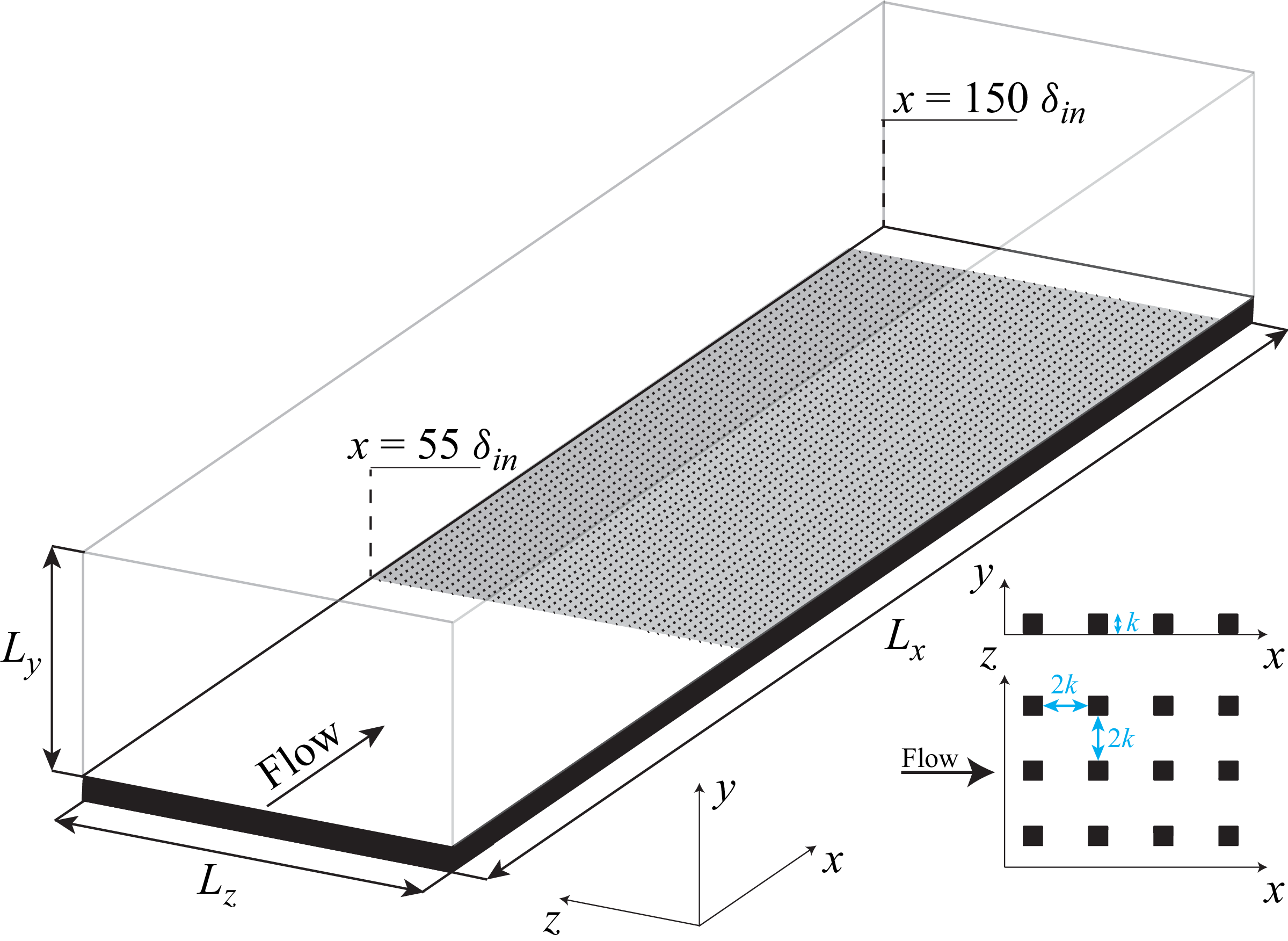
 k
k 2k
2k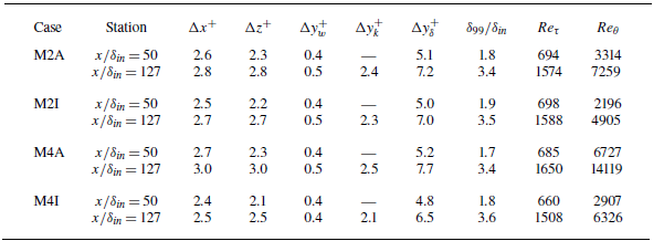
 Δx+
Δx+ Δz+
Δz+ Δyw+
Δyw+ Δyk+
Δyk+ Δyδ+
Δyδ+ Reθ=ρ∞u∞θ/μ∞
 θ
θ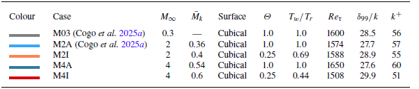
 x=127δin
 Θ=(Tw−T∞)/(Tr−T∞)
 Tw/Tr
Tw/Tr Reτ=ρwuτδ99/μw
 k
k M¯k
M¯k δ99
δ99 u¯/u∞=0.99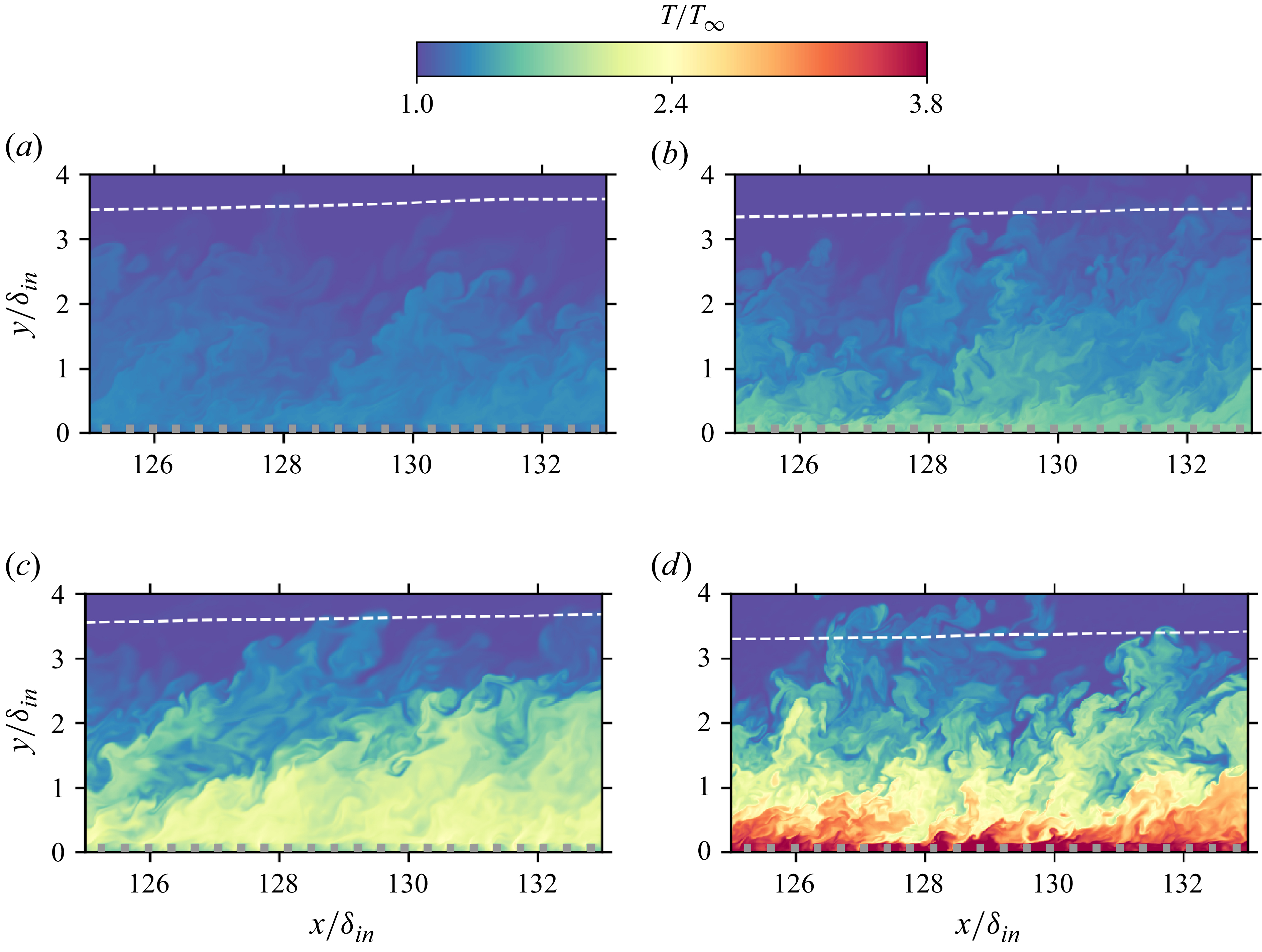
 T/T∞
T/T∞ x
x y
y δ99
δ99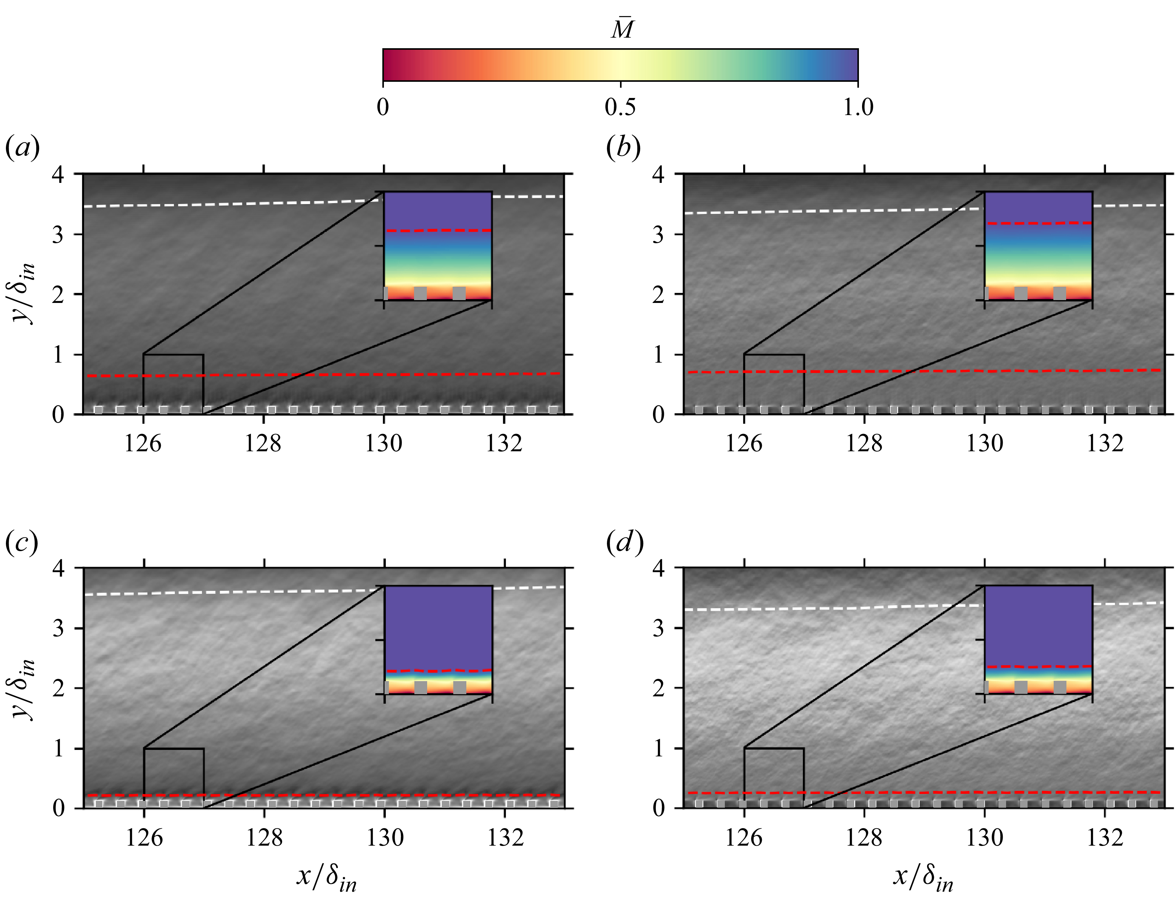
 exp(−100|∇ρ¯|)
 ρ¯/ρ∞
ρ¯/ρ∞ x
x y
y 0.5
0.5 1.1
1.1 δ99
δ99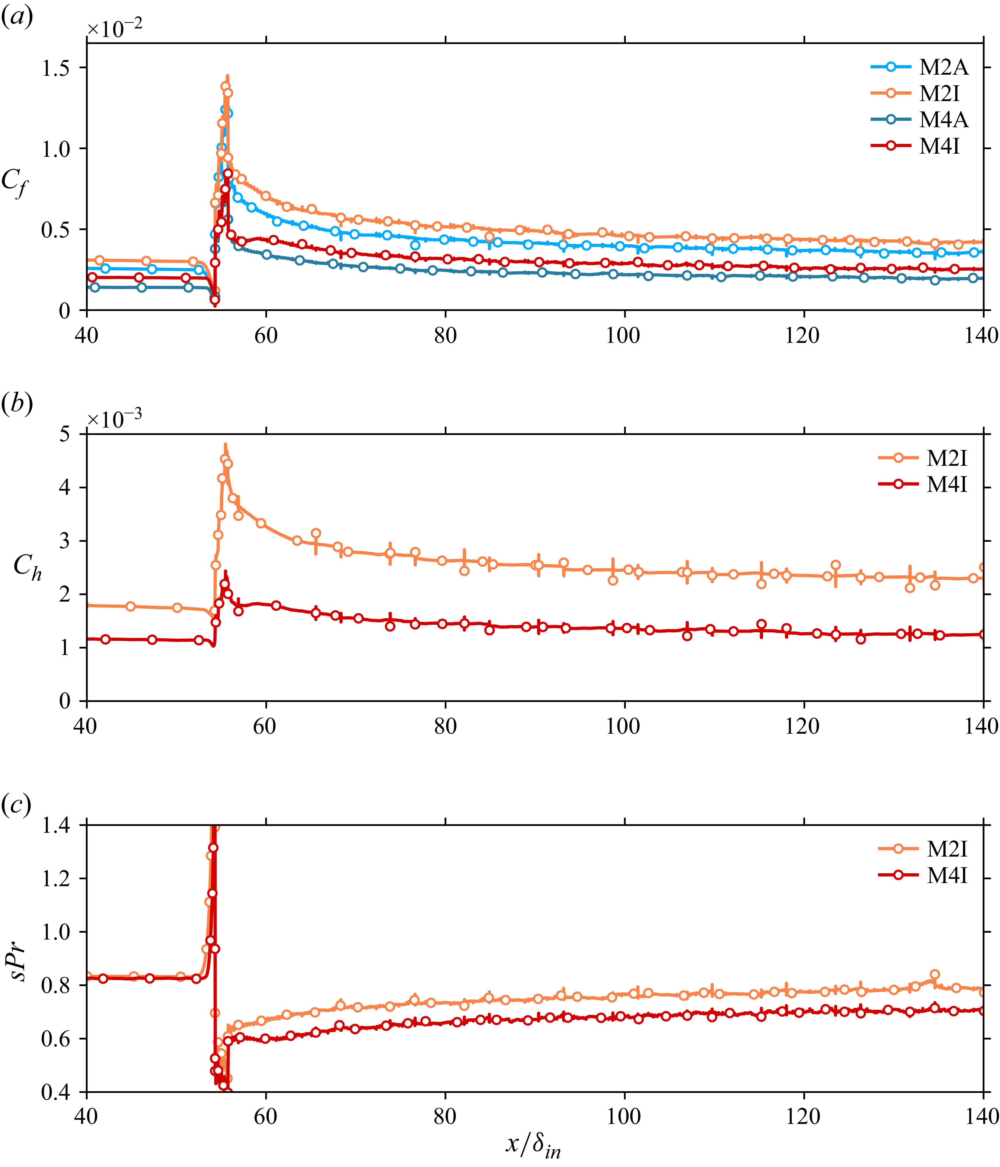
 Cf=τw/(1/2ρ∞u∞2)
 Ch=qw/(ρ∞u∞cp(Tw−Tr))
 sPr=2Ch/CfPr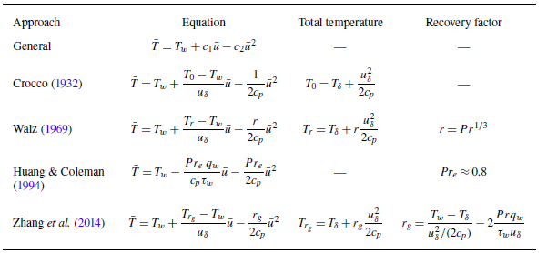
 qw/τw
qw/τw sPr=2Ch/CfPr≈0.8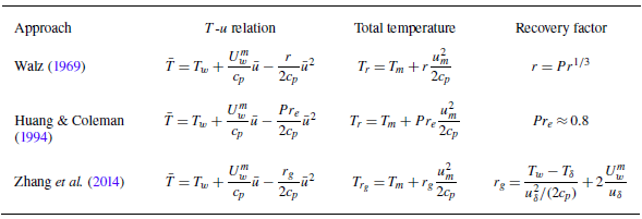
 Uwm
Uwm c1
c1 c2
c2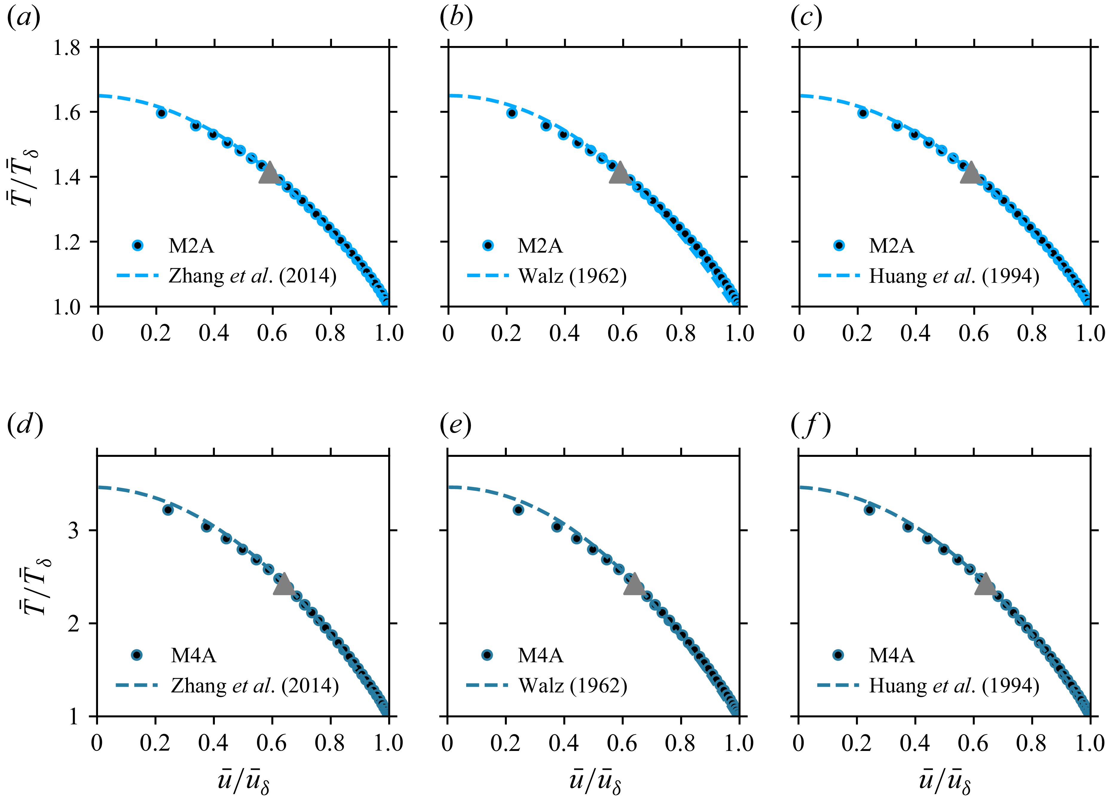
 x=127δin
 y+=300
 qw
qw τw
τw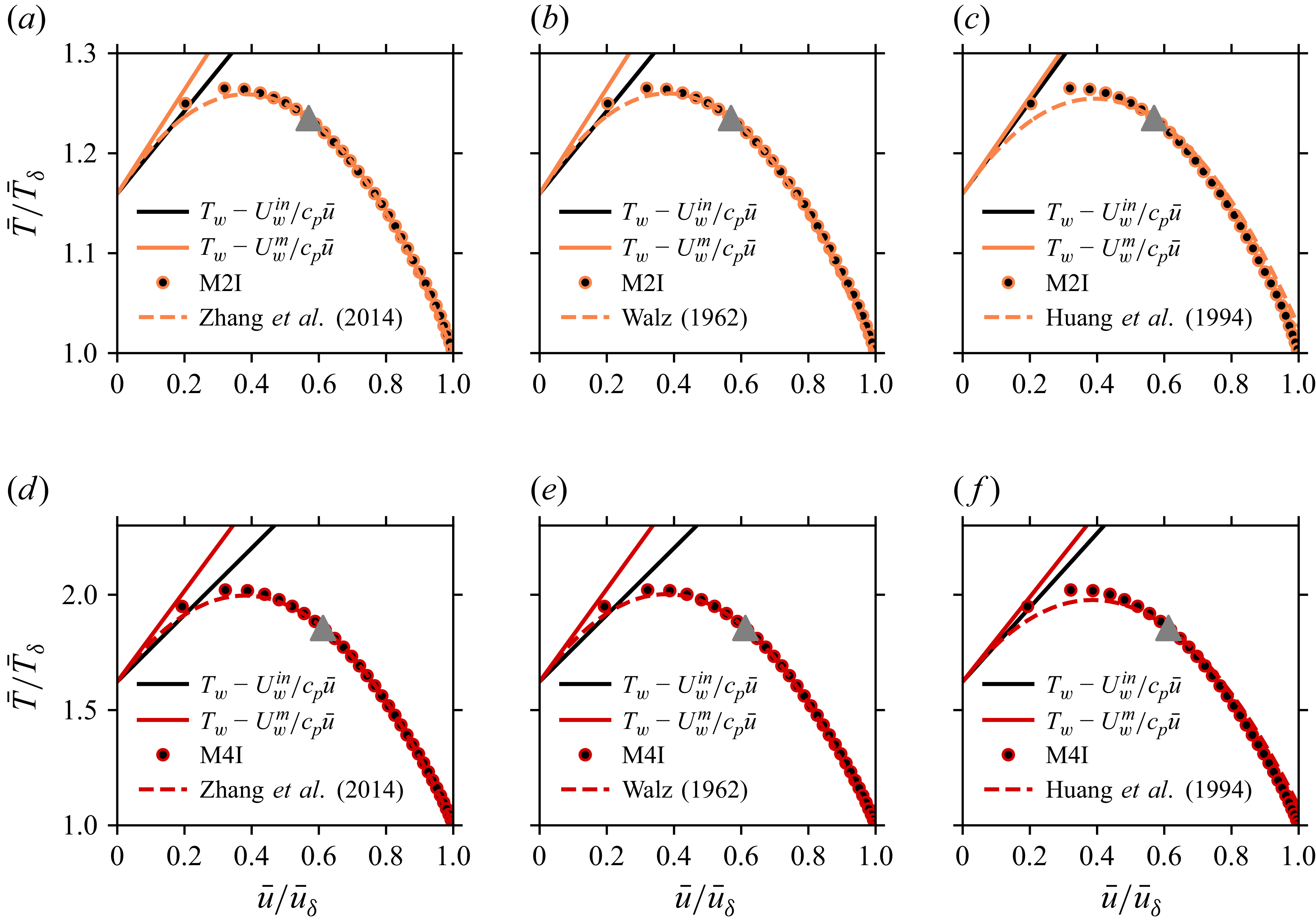
 x=127δin
 y+=300
 ∂T/∂u|w=Uw/cp
 Uwm
Uwm Uwin
Uwin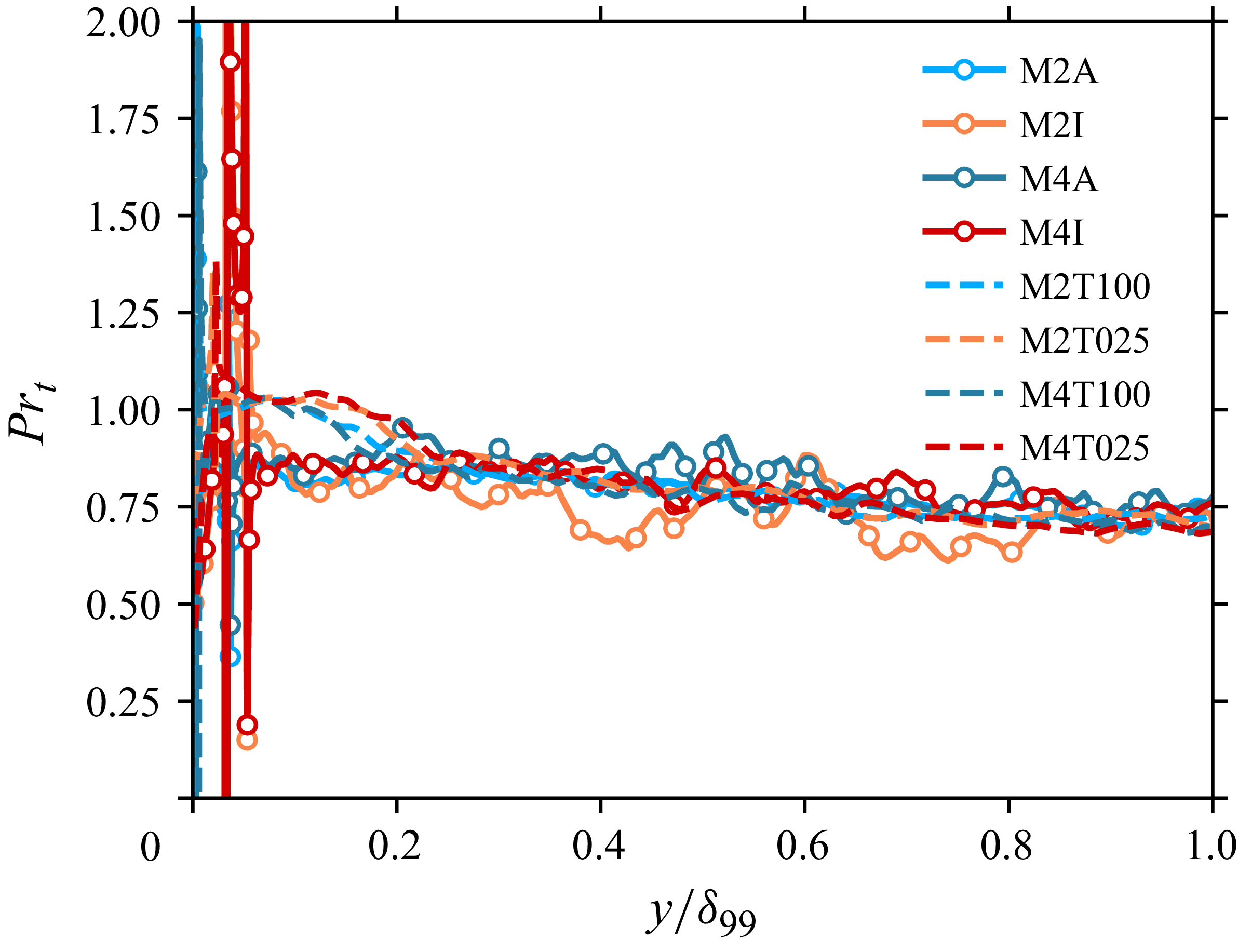
 Prt
Prt y/δ99
y/δ99 Reτ=443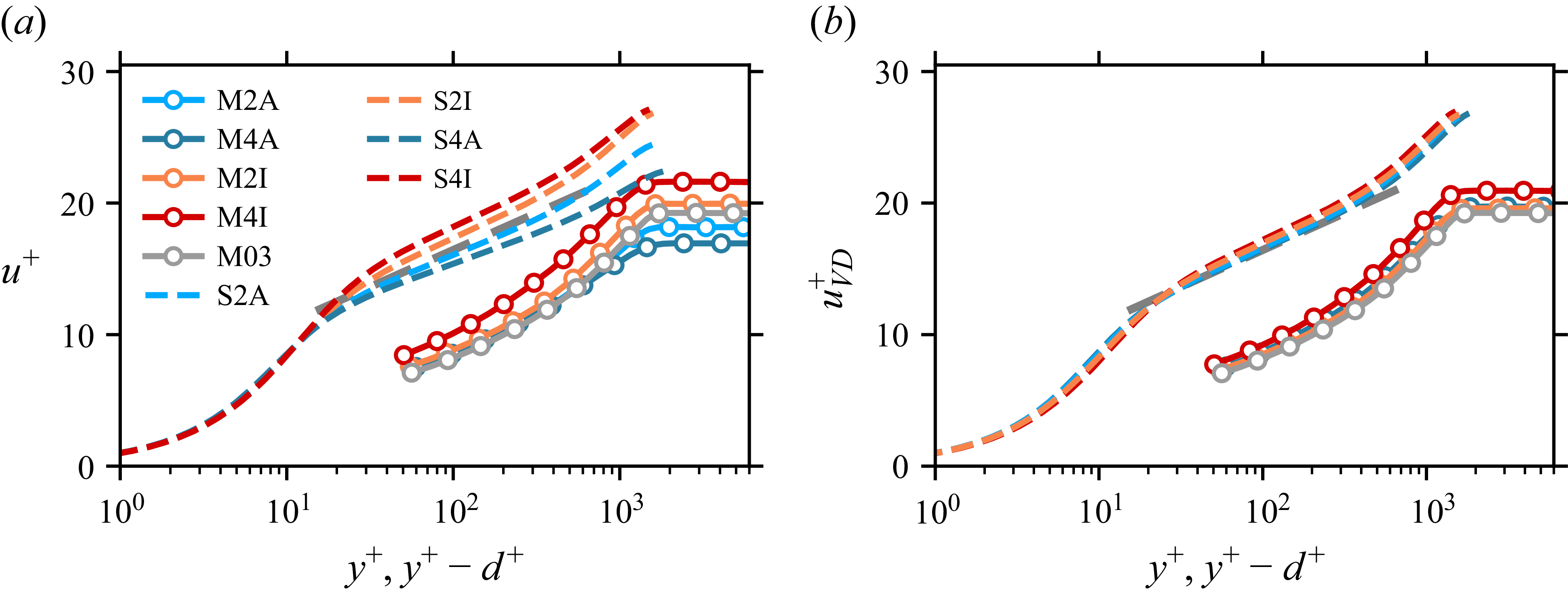
 u+
u+ y+
y+ d
d u+=(1/κ) ln(y+)+5.2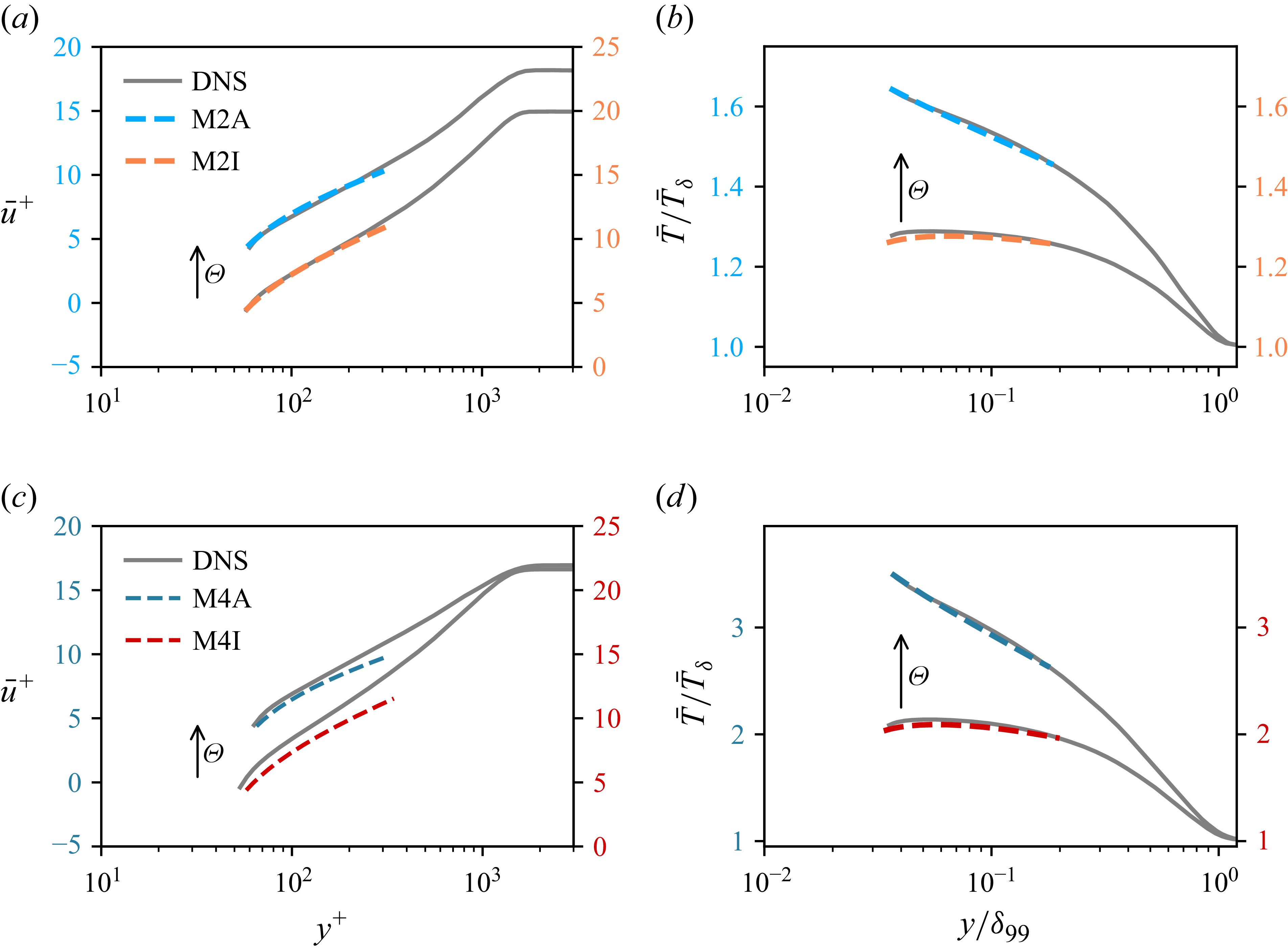
 y+
y+ y/δ99
y/δ99 M∞=2
M∞=2 M∞=4
M∞=4 Θ≈1
Θ≈1 Θ=0.25
 Δu+=5
Δu+=5 ym+=300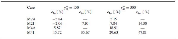
 ym+=150
 ym+=300
 ϵτw=(τw,model−τw,DNS)/τw,DNS×100
 ϵqw=(qw,model−qw,DNS)/qw,DNS×100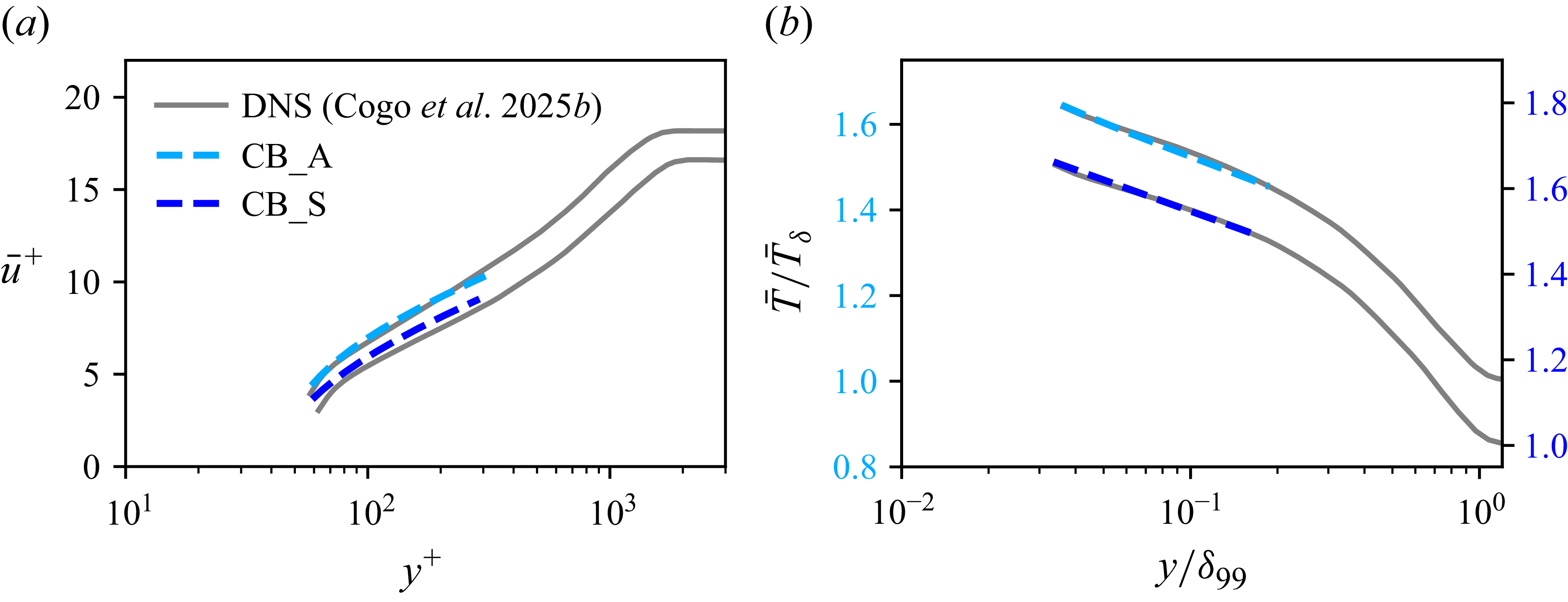
 y+
y+ y/δ99
y/δ99 M∞=2
M∞=2 ΔT=0.15
 ym+=300
 Open access

