


1. Introduction
We study an initial-boundary value problem for
 $(A, \rho , u)$
, defined on the space-time domain
$(A, \rho , u)$
, defined on the space-time domain
 $(\textbf {x}, t) \in \Omega \times (0, T]$
, where
$(\textbf {x}, t) \in \Omega \times (0, T]$
, where
 $\Omega \subset \mathbb{R}^N$
is a bounded domain with piecewise smooth boundary
$\Omega \subset \mathbb{R}^N$
is a bounded domain with piecewise smooth boundary
 $\partial \Omega$
, and the time horizon
$\partial \Omega$
, and the time horizon
 $T\gt 0$
 \begin{equation} \left \{ \begin{aligned} \frac {\partial A}{\partial t}=&\,D_A\Delta A - A+\alpha +A\rho , &&\text{ in } \Omega \times (0, T], \\[5pt] \frac {\partial \rho }{\partial t}=&\,\nabla \cdot \left (D_\rho \nabla \rho -2 \rho \nabla \ln A\right )-A\rho +\beta - \rho u, &&\text{ in } \Omega \times (0, T], \\[5pt] \frac {\partial u}{\partial t}=&\,\nabla \cdot \left (D_u \nabla u-\chi u\nabla \ln A\right ), &&\text{ in } \Omega \times (0, T], \\[5pt] \frac {\partial A}{\partial \textbf {n}}=&\, \frac {\partial \rho }{\partial \textbf {n}}= \frac {\partial u}{\partial \textbf {n}}=0, &&\text{ on }\partial \Omega , \\[5pt] (A, \rho , u)&(\textbf {x}, 0)=(A_0, \rho _0, u_0)\geq , \not \equiv 0, && \text{ in }\Omega . \end{aligned} \right . \end{equation}
Here,
 $\partial$
denotes partial differentiation with respect to time
$\partial$
denotes partial differentiation with respect to time
 $t$
, while
$t$
, while
 $\nabla$
and
$\nabla$
and
 $\Delta$
represent the spatial gradient and Laplacian operators, respectively. The parameters
$\Delta$
represent the spatial gradient and Laplacian operators, respectively. The parameters
 $D_A, D_\rho , D_u, \alpha ,$
and
$D_A, D_\rho , D_u, \alpha ,$
and
 $\beta$
are assumed to be positive constants, whereas
$\beta$
are assumed to be positive constants, whereas
 $\chi$
may take either positive or negative values, depending on the modelling context, as discussed later. The zero-flux (Neumann) boundary conditions, expressed via
$\chi$
may take either positive or negative values, depending on the modelling context, as discussed later. The zero-flux (Neumann) boundary conditions, expressed via
 $\frac {\partial }{\partial \mathbf{n}}$
, are imposed to model an enclosed environment. The initial conditions are assumed to be nonnegative and not identically zero; this, together with the strong maximum principle, ensures that each component
$\frac {\partial }{\partial \mathbf{n}}$
, are imposed to model an enclosed environment. The initial conditions are assumed to be nonnegative and not identically zero; this, together with the strong maximum principle, ensures that each component
 $(A, \rho , u)$
remains strictly positive for all
$(A, \rho , u)$
remains strictly positive for all
 $t \gt 0$
. Finally, the terminal time
$t \gt 0$
. Finally, the terminal time
 $T$
represents the time horizon for the analysis: it is taken as infinite in theoretical investigations and sufficiently large in numerical simulations to capture the system’s long-term behaviour.
$T$
represents the time horizon for the analysis: it is taken as infinite in theoretical investigations and sufficiently large in numerical simulations to capture the system’s long-term behaviour.
1.1. The UCLA model
System (E) can be used to model the spatio-temporal evolution of urban criminal activity under the influence of police patrol intervention. Specifically, it describes the dynamics of the population density
 $\rho$
of criminal agents, who are attracted to regions with high attractiveness
$\rho$
of criminal agents, who are attracted to regions with high attractiveness
 $A$
and are deterred by the presence of law enforcement, represented by
$A$
and are deterred by the presence of law enforcement, represented by
 $u$
. This approach to modelling urban crime traces back to the seminal work [Reference Short, D’orsogna and Pasour48] of a UCLA team in 2008, which was inspired by theories such as routine activity theory, the broken-windows effect and the repeat and near-repeat victimization effect [Reference Sampson and Raudenbush43, Reference Wilson and Kelling60]. They developed a two-dimensional agent-based lattice model that captures both the movement of offenders and the evolution of local attractiveness. In the spatial continuum limit, this discrete model leads to a fully coupled system of partial differential equations:
$u$
. This approach to modelling urban crime traces back to the seminal work [Reference Short, D’orsogna and Pasour48] of a UCLA team in 2008, which was inspired by theories such as routine activity theory, the broken-windows effect and the repeat and near-repeat victimization effect [Reference Sampson and Raudenbush43, Reference Wilson and Kelling60]. They developed a two-dimensional agent-based lattice model that captures both the movement of offenders and the evolution of local attractiveness. In the spatial continuum limit, this discrete model leads to a fully coupled system of partial differential equations:
 \begin{equation} \left \{ \begin{aligned} \frac {\partial A}{\partial t}=&\,D_A\Delta A - A+A_0+A\rho , &&\text{ in } \Omega \times (0, T], \\[5pt] \frac {\partial \rho }{\partial t}=&\,\nabla \cdot (D_\rho \nabla \rho -2 \rho \nabla \ln A)-A\rho +\bar B, &&\text{ in } \Omega \times (0, T]. \end{aligned} \right . \end{equation}
The linear diffusion coefficient
 $D_A$
represents the effect of the near-repeat victimization phenomenon. Since the expected number of crimes is given by the product
$D_A$
represents the effect of the near-repeat victimization phenomenon. Since the expected number of crimes is given by the product
 $A\rho$
, the self-exciting nature of crime is incorporated into the dynamics through the
$A\rho$
, the self-exciting nature of crime is incorporated into the dynamics through the
 $+A\rho$
term in the first equation. When a crime occurs, it is assumed that the perpetrator is removed, leading to the
$+A\rho$
term in the first equation. When a crime occurs, it is assumed that the perpetrator is removed, leading to the
 $-A\rho$
term in the second equation. External sources of growth, which may vary in space and time, are also considered for both variables and are denoted by
$-A\rho$
term in the second equation. External sources of growth, which may vary in space and time, are also considered for both variables and are denoted by
 $A_0$
and
$A_0$
and
 $\bar {B}$
, respectively. Finally, we note that the movement of offenders combines random motion, modelled by linear diffusion, with a directional bias towards regions of high attractiveness – resulting in a chemotaxis-like drift. We refer interested readers to [Reference Gu, Wang and Yi19, Reference Short, D’orsogna and Pasour48] for detailed derivations and further justification of system (1.1.1) and to [Reference D’Orsogna and Perc12, Reference Groff, Johnson and Thornton18] for reviews of agent-based models in urban crime modelling.
$\bar {B}$
, respectively. Finally, we note that the movement of offenders combines random motion, modelled by linear diffusion, with a directional bias towards regions of high attractiveness – resulting in a chemotaxis-like drift. We refer interested readers to [Reference Gu, Wang and Yi19, Reference Short, D’orsogna and Pasour48] for detailed derivations and further justification of system (1.1.1) and to [Reference D’Orsogna and Perc12, Reference Groff, Johnson and Thornton18] for reviews of agent-based models in urban crime modelling.
The UCLA continuum model and its 2D lattice counterpart have gained significant academic recognition for their ability to simulate complex spatio-temporal dynamics and generate both regular and irregular spatial patterns. Most notably, these models successfully capture the aggregation phenomena, commonly known as hotspots, in urban criminal activity, providing critical insights into the spatial distribution of crime. The global well-posedness of the model in (1.1.1) is investigated in [Reference Freitag14, Reference Jiang and Wang21, Reference Rodríguez38, Reference Rodríguez and Winkler40, Reference Wang, Wang and Feng55, Reference Winkler61]. These studies have established that the system admits a unique global-in-time solution, which remains uniformly bounded in one-dimensional settings or in higher dimensions when the advection effect is weak or sublinear. More importantly, a substantial body of research, including [Reference Berestycki, Wei and Winter4, Reference Cantrell, Cosner and Manásevich8, Reference Garcia-Huidobro, Manasevich and Mawhin17, Reference Gu, Wang and Yi19, Reference Heihoff20, Reference Kolokolnikov, Ward and Wei24, Reference Lloyd and O’Farrell28, Reference Lloyd, Santitissadeekorn and Short29, Reference Manasevich, Phan and Souplet30, Reference Mei and Wei32, Reference Short, Bertozzi and Brantingham46, Reference Short, Brantingham, Bertozzi and Tita47, Reference Tse and Ward53], has focused on the emergence of nontrivial spatial patterns. These works demonstrate that system (1.1.1) can produce structured crime hotspots, represented by spatially concentrated profiles that may be either stationary or time-dependent, thereby successfully capturing the characteristic features of urban residential burglary. Building on these foundations, researchers have extended the theoretical framework of system (1.1.1) to model real-world crime dynamics more accurately. They include the study of non-linear or anomalous diffusion and spatial heterogeneity in both the near-repeat victimization effect and the dispersal strategies of offenders [Reference Gu, Wang and Yi19, Reference Martínez-Farías, Alvarado-Sánchez, Rangel-Cortes and Hernández-Hernández31]; modelling criminal movement using Lévy processes [Reference Chaturapruek, Breslau, Yazdi, Kolokolnikov and McCalla9, Reference Levajković, Mena and Zarfl27, Reference Pan, Li and Wang35]; incorporating age-structured populations [Reference Kumar and Abbas25, Reference Saldana, Aguareles, Avinyó, Pellicer and Ripoll42] and examining geographic profiling [Reference Mohler and Short33]. For reviews in this area, we refer the reader to [Reference Berestycki and Nadal3, Reference Berestycki, Wei and Winter4, Reference D’Orsogna and Perc12, Reference Mohler, Short, Brantingham, Schoenberg and Tita34].
1.2. The UCLA model with policing force
Given that crime and disorder are unevenly distributed across urban areas, scholars and practitioners in [Reference Eck, Farrington, MacKenzie, Sherman and Welsh13, Reference Frydl and Skogan15, Reference Sherman and Weisburd44, Reference Skogan and Hartnett49, Reference Weisburd and Eck57, Reference Weisburd and Green58] have advocated for concentrating policing efforts in high-demand zones rather than dispersing resources uniformly across the city. This strategy, commonly referred to as “hot-spot policing” or “hotspotting, ” emphasizes geographic precision, focusing on the location of crimes rather than the characteristics of individual offenders. While this targeted approach has demonstrated measurable short-term reductions in crime, its broader effectiveness remains the subject of debate. Critics (cf., [Reference Braga5, Reference Braga, Papachristos and Hureau6, Reference Frydl and Skogan15, Reference Kleck and Barnes23, Reference Rosenbaum, Weisburd and Braga41, Reference Weisburd, Telep, Hinkle and Eck59]) have raised concerns about potential unintended consequences, such as the spatial displacement of crime, the erosion of community trust and the risk of over-policing marginalized neighbourhoods. Moreover, questions remain about how different policing strategies interact with the underlying social and economic dynamics that drive criminal behaviour. These challenges highlight the need for more comprehensive models that not only track where crime occurs but also capture how policing interventions influence the evolving spatial patterns of crime over time.
A major extension of the original model proposed by the UCLA team involves incorporating the effects of policing strategies on the evolution of criminal activity. In particular, the authors of [Reference Jones, Brantingham and Chayes22, Reference Pitcher36] independently introduced an additional equation to represent police deployment and targeted patrols. These papers adopt different modelling frameworks and assign distinct roles to law enforcement. In this work, we follow the formulation introduced in the later study [Reference Tse and Ward54], which in turn builds on the continuum model of [Reference Ricketson37], itself a generalization of the earlier approach in [Reference Pitcher36]:
 \begin{equation*} u_t=\nabla \cdot (D_u\nabla u-\chi u\nabla \ln A), \end{equation*}
where
 $u$
denotes the distribution of law enforcement in the field. The positive parameters
$u$
denotes the distribution of law enforcement in the field. The positive parameters
 $D_u$
and
$D_u$
and
 $\chi$
represent the intensity of the random movement of police and their response to criminal activity, respectively. Incorporating an explicit law enforcement component allows one to systematically study how various patrol strategies, whether reactive or proactive, affect hotspot formation, stability and suppression under different assumptions about agent movement and crime-attractiveness feedback. When
$\chi$
represent the intensity of the random movement of police and their response to criminal activity, respectively. Incorporating an explicit law enforcement component allows one to systematically study how various patrol strategies, whether reactive or proactive, affect hotspot formation, stability and suppression under different assumptions about agent movement and crime-attractiveness feedback. When
 $\chi \gt 0$
, law enforcement agents tend to migrate towards areas with high attractiveness, whereas
$\chi \gt 0$
, law enforcement agents tend to migrate towards areas with high attractiveness, whereas
 $\chi \lt 0$
corresponds to a strategy in which police are deployed to regions of low attractiveness.
$\chi \lt 0$
corresponds to a strategy in which police are deployed to regions of low attractiveness.
From a modelling perspective, one may question the realism of choosing
 $\chi \lt 0$
. In particular, it remains unclear whether deploying police resources to low-crime areas yields clear benefits [Reference Barthe and Stitt2]. Nevertheless, we allow
$\chi \lt 0$
. In particular, it remains unclear whether deploying police resources to low-crime areas yields clear benefits [Reference Barthe and Stitt2]. Nevertheless, we allow
 $\chi \lt 0$
in our formulation to avoid imposing additional constraints solely to guarantee positivity. We also identify a second important threshold at
$\chi \lt 0$
in our formulation to avoid imposing additional constraints solely to guarantee positivity. We also identify a second important threshold at
 $\chi = 2$
, corresponding to the regime in which police movement matches that of crime agents. The two values
$\chi = 2$
, corresponding to the regime in which police movement matches that of crime agents. The two values
 $\chi = 0$
and
$\chi = 0$
and
 $\chi = 2$
will therefore play a central role in the numerical simulations presented in this paper. In addition, we identify other critical
$\chi = 2$
will therefore play a central role in the numerical simulations presented in this paper. In addition, we identify other critical
 $\chi$
-thresholds associated with the onset of various bifurcations. Together, these critical parameter values determine the qualitative behaviour of the system. Consequently, changes in police response intensity may fundamentally reshape the spatial crime landscape. The sign and magnitude of
$\chi$
-thresholds associated with the onset of various bifurcations. Together, these critical parameter values determine the qualitative behaviour of the system. Consequently, changes in police response intensity may fundamentally reshape the spatial crime landscape. The sign and magnitude of
 $\chi$
thus encode different policing strategies and can be chosen according to the specific modelling objectives.
$\chi$
thus encode different policing strategies and can be chosen according to the specific modelling objectives.
While adding a third equation to model law enforcement enhances the system’s realism by incorporating police deployment strategies, it also introduces new mathematical challenges, particularly in analysing pattern formation and stability. The resulting three-component reaction–diffusion system (E) has been examined by several researchers to explore how policing influences crime dynamics. Tse and Ward [Reference Tse and Ward54] conducted a detailed singular perturbation analysis of (E) in one dimension, constructing steady-state hotspot (spike) solutions and performing a nonlocal eigenvalue analysis to characterize their linear stability. They distinguished between synchronous and asynchronous instabilities, showing that hotspot locations may destabilize either in phase (oscillating together) or out of phase (oscillating asynchronously), depending on police response and other system parameters. These results highlight how law enforcement strategies shape the temporal dynamics of urban crime distributions. Building on this foundation, Buttenschoen et al. [Reference Buttenschoen, Kolokolnikov, Ward and Wei7] refined the linear stability framework and focused more explicitly on how targeted policing strategies influence hotspot selection and stabilization. Their work strengthens the connection between the number and spacing of spikes and the intensity of police deployment, demonstrating, for example, that increasing the strength or spatial focus of policing can shift the threshold for hotspot instability.
Rodríguez et al. [Reference Rodríguez, Wang and Zhang39] applied bifurcation theory to rigorously establish the existence of stable spatial and temporal patterns (steady states and periodic orbits), identify critical thresholds for pattern emergence and analyse wavemode selection. Strikingly, they showed that anti-hotspot policing – dispatching police away from areas of high attractiveness – can stabilize crime hotspots and suppress oscillations. Although they proved global existence and boundedness of solutions, their analysis also revealed that the system may exhibit ill-posedness due to strong sensitivity to initial conditions, raising concerns about its predictive reliability. Further studies of system (E) can be found in [Reference Gai and Ward16, Reference Ricketson37, Reference Yerlanov, Wang and Rodríguez62, Reference Zipkin, Short and Bertozzi63], where the extended model has been examined under different contexts. Collectively, these works demonstrate that the system supports a broad spectrum of dynamic behaviours – including spatially uniform equilibria, spatially heterogeneous steady states, periodic oscillations and even chaotic patterns. Numerical simulations across the literature not only validate the theoretical predictions but also underscore the model’s inherent richness and complexity.
1.3. Preliminaries and outline
Before detailing our main steps and contributions, we first note that in this framework, homogeneous Neumann boundary conditions imply a fixed number of guardians throughout all temporal dynamics as
 \begin{equation*}\frac {d}{dt}\int _\Omega u(\textbf {x}, t)d\textbf {x}=0\quad \forall t\gt 0.\end{equation*}
If we introduce a parameter
 $\lambda$
to represent the spatial average of
$\lambda$
to represent the spatial average of
 $A$
, then the system admits the following positive constant steady state
$A$
, then the system admits the following positive constant steady state
 \begin{equation} \bar {A} \;:\!=\;\lambda , \;\; \bar {\rho } \;:\!=\;1-\frac {\alpha }{\lambda }, \;\; {\bar {u}} \;:\!=\;\frac {1}{|\Omega |}\int _\Omega u_0(\textbf {x})\;d\textbf {x}= \lambda \left (\frac {\beta }{\lambda -\alpha }-1\right ), \end{equation}
each of which is positive under the condition
 \begin{equation*} \alpha \lt \lambda \lt \alpha +\beta . \end{equation*}
Our study focuses on spatially heterogeneous solutions of system (E) that extend beyond the homogeneous patterns described by (SS). To characterize the system’s long-term behaviour, we analyse its steady states, natural candidates for dynamical attractors, by seeking nonconstant positive solutions to the following coupled system:
 \begin{equation} \left \{ \begin{aligned} &0=D_A\Delta A - A+\alpha +A\rho , &&\text{ in } \Omega , \\[5pt] &0=\nabla \cdot ({D_\rho \nabla \rho }- 2 \rho \nabla \ln A)-A\rho +\beta - \rho u, &&\text{ in } \Omega , \\[5pt] &0=\nabla \cdot ({D_u \nabla u}-\chi u\nabla \ln A), &&\text{ in } \Omega , \\[5pt] &\frac {\partial A}{\partial \textbf {n}}= \frac {\partial \rho }{\partial \textbf {n}}= \frac {\partial u}{\partial \textbf {n}}=0, &&\text{ on }\partial \Omega . \end{aligned} \right . \end{equation}
The interaction between spatial heterogeneity and non-linear coupling creates significant mathematical challenges, and a deeper analysis is needed to fully understand the resulting dynamics. While prior studies in [Reference Buttenschoen, Kolokolnikov, Ward and Wei7, Reference Gai and Ward16, Reference Rodríguez, Wang and Zhang39, Reference Tse and Ward54, Reference Zipkin, Short and Bertozzi63] have shown the existence of spatially heterogeneous solutions, most focus on one-dimensional domains or simplified models, leaving open the problem of rigorous higher-dimensional analysis. This work addresses that gap by extending the framework of [Reference Rodríguez, Wang and Zhang39] to higher dimensions and by developing a general approach for bifurcation analysis in three-agent systems on spatial domains. To do so, the paper follows the framework presented in [Reference Cantrell, Cosner and Manásevich8], where bifurcation analysis was done on a two-component system (1.1.1). Essentially, this paper should be viewed as a convergence of two works [Reference Cantrell, Cosner and Manásevich8, Reference Rodríguez, Wang and Zhang39], extending in both the number of components and the dimension of the underlying geometry. We establish the Crandall–Rabinowitz theorem and stability results for systems with guardians in any spatial dimension, using Laplacian eigenvalues rather than wave-mode numbers (Theorems2.2, 3.1). Our proofs are given in explicit detail, making the methods adaptable to other three-agent systems. We also generalize the Hopf bifurcation theorem to higher dimensions [Reference Amann, Busenberg and Martelli1] (Theorem4.1). On the computational side, we provide parameter-based verification guided by linear stability analysis and include simulations in both one- and two-dimensional dimensions. These simulations highlight features such as long transients and consistent behaviours across dimensions. We further demonstrate chaotic dynamics using bifurcation diagrams and perform a systematic parameter sweep to explore how parameter magnitudes affect system outcomes. Together, these results provide a comprehensive and general treatment of the target–guardian–offender model.
This work develops its analysis through three sequential components: first, a linear stability examination of the constant solution (SS) establishes the baseline conditions for pattern formation; second, a steady state bifurcation analysis reveals how intensive guardians drive the emergence of nontrivial solutions from this trivial state and third, a Hopf bifurcation analysis locating the onset of oscillatory behaviour and proving the existence of periodic solutions. Finally, we complement our theoretical results with numerical simulations that not only validate our predictions but also reveal complex, chaotic dynamics. These simulations highlight the rich pattern formation potential of the extended system and demonstrate behaviours not previously captured in earlier models.
2. Steady state bifurcation analysis
In this section, we perform a bifurcation analysis to demonstrate the existence of non-constant steady-state solutions, thereby showing that the system can generate stable spatial patterns under suitable conditions. The main idea is to translate the problem into an equivalent linear algebra setting and carry out the analysis there. In [Reference Crandall and Rabinowitz10], this approach is applied to a two–component system, where the corresponding algebra is simpler; for instance, the determinant of a
 $2 \times 2$
matrix has a closed-form expression, unlike the
$2 \times 2$
matrix has a closed-form expression, unlike the
 $3 \times 3$
case considered here. Following the framework of [Reference Crandall and Rabinowitz10], we emphasize the additional steps needed to address these higher–dimensional algebraic challenges.
$3 \times 3$
case considered here. Following the framework of [Reference Crandall and Rabinowitz10], we emphasize the additional steps needed to address these higher–dimensional algebraic challenges.
For the sake of simplicity, we shift the scalar fields in system (E) using the steady state (SS) by setting
 \begin{equation*} \tilde A(\textbf {x}, t)\;:\!=\;A(\textbf {x}, t)-\bar A, \quad \tilde \rho (\textbf {x}, t)\;:\!=\;\rho -\bar \rho , \quad \tilde u(\textbf {x}, t)\;:\!=\;u(\textbf {x}, t)-\bar u. \end{equation*}
and collect the following the equivalent system for
 $(\bar {A}, \bar {\rho }, \bar {u})$
 \begin{align} \left \{ \begin{aligned} \frac {\partial \tilde {A}}{\partial t}=&\,D_A\Delta \tilde {A} - \tilde {A}+\tilde {A}\tilde {\rho } +\bar {\rho }\tilde {A}+ \bar {A}\tilde {\rho }+\bar {A}\bar {\rho }+\alpha , &&\text{ in }\Omega \times (0, T], \\[5pt] \frac {\partial \tilde {\rho }}{\partial t}=&\,\nabla \cdot (D_\rho \nabla \tilde {\rho } - \frac {2(\tilde {\rho }+\bar {\rho })}{\tilde {A}+\bar {A}}\nabla \tilde {A})&&\\[5pt] &- \tilde {A} \tilde {\rho }-\bar {A} \tilde {\rho }-\bar {\rho }\tilde {A}-\tilde {\rho }\tilde {u}-{\bar {u}}\tilde {\rho }-\bar {\rho }\tilde {u}+\beta -\bar {\rho }({\bar {u}}+\bar {A}), &&\text{ in }\Omega \times (0, T], \\[5pt] \frac {\partial \tilde {u}}{\partial t}=&\,\nabla \cdot \left(D_u \nabla \tilde {u} - \frac {\chi (\tilde {u}+{\bar {u}})}{\tilde {A}+\bar {A}}\nabla \tilde {A}\right), &&\text{ in }\Omega \times (0, T], \\[5pt] \frac {\partial \tilde A}{\partial \textbf {n}}=&\, \frac {\partial \tilde \rho }{\partial \textbf {n}}= \frac {\partial \tilde u}{\partial \textbf {n}}=0, &&\text{ on }\partial \Omega . \end{aligned} \right . \end{align}
This new system (ME) has a shifted equilibrium
 $\mathbf{0}\;:\!=\;(0, 0, 0)$
, and dropping tildes we obtain
$\mathbf{0}\;:\!=\;(0, 0, 0)$
, and dropping tildes we obtain
 \begin{equation} \left \{ \begin{aligned} \frac {\partial A}{\partial t}=&\,D_A\Delta A - A +A\rho +\left (1-\frac {\alpha }{\lambda }\right )A+\lambda \rho , &&\quad \text{ in }\Omega \times (0, T], \\[5pt] \frac {\partial \rho }{\partial t}=&\,\nabla \cdot \Big (D_\rho \nabla \rho - \frac {2\left (\rho +\left (1-\frac {\alpha }{\lambda }\right )\right )}{A+\lambda }\nabla A\Big )- A \rho -\lambda \rho &&\\[5pt] &-\left (1-\frac {\alpha }{\lambda }\right )A-\rho u-\rho \lambda \left (\frac {\beta }{\lambda -\alpha }-1\right )-u\left (1-\frac {\alpha }{\lambda }\right ), &&\quad \text{ in }\Omega \times (0, T], \\[5pt] \frac {\partial u}{\partial t}=&\,\nabla \cdot \Big (D_u \nabla u - \frac {\chi \left (u+\lambda \left (\frac {\beta }{\lambda -\alpha }-1\right )\right )}{A+\lambda }\nabla A\Big ), &&\quad \text{ in }\Omega \times (0, T], \\[5pt] \frac {\partial A}{\partial \textbf {n}}=&\, \frac {\partial \rho }{\partial \textbf {n}}= \frac {\partial u}{\partial \textbf {n}}=0, &&\quad \text{ on }\partial \Omega . \end{aligned} \right . \end{equation}
We now aim to study the steady-state solutions of system (MP), and to this end, we introduce the operator
 $\mathcal F$
as follows
$\mathcal F$
as follows
 \begin{equation} \begin{split} &\mathcal F(\chi , A, \rho , u)\\[5pt] \;:\!=\;&\begin{bmatrix} D_A\Delta A+A\rho -\frac {\alpha }{\lambda }A+\lambda \rho \\[5pt] \nabla \cdot \left [D_\rho \nabla \rho - \frac {2\left (\rho +\left (1-\frac {\alpha }{\lambda }\right )\right )}{A+\lambda }\nabla A\right ]- A \rho -\lambda \rho -\left (1-\frac {\alpha }{\lambda }\right )A-\rho u-\rho \lambda \left (\frac {\beta }{\lambda -\alpha }-1\right )-u\left (1-\frac {\alpha }{\lambda }\right )\\[5pt] \nabla \cdot \left [D_u \nabla u - \frac {\chi \left (u+\lambda \left (\frac {\beta }{\lambda -\alpha }-1\right )\right )}{A+\lambda }\nabla A\right ] \end{bmatrix}. \end{split} \end{equation}
Then,
 $\mathcal F(\chi , \mathbf{0})=0$
for any
$\mathcal F(\chi , \mathbf{0})=0$
for any
 $\chi \in \mathbb{R}$
, and we are motivated to find nontrivial equilibria of (MP) that bifurcate from the trivial one. It is equivalent to solving the following problem
$\chi \in \mathbb{R}$
, and we are motivated to find nontrivial equilibria of (MP) that bifurcate from the trivial one. It is equivalent to solving the following problem
 \begin{equation} \mathcal F(\chi , A, \rho , u)=0, \quad \chi \in \mathbb R,\quad (A, \rho , u)\in \mathcal Y, \end{equation}
where
 \begin{equation*} \mathcal Y=\left \{(A, \rho , u)\in [H^2(\Omega )]^3\Big |\;\frac {\partial A}{\partial \textbf {n}}=\frac {\partial \rho }{\partial \textbf {n}}=\frac {\partial u}{\partial \textbf {n}}=0\text{ on }\partial \Omega , \, \int _\Omega u d\textbf {x}=0\right \}. \end{equation*}
Indeed, any root of
 $\mathcal{F} = 0$
is known to be a weak solution of (2.0.1), and standard elliptic regularity theory then ensures that this weak solution is, in fact, classical and smooth.
$\mathcal{F} = 0$
is known to be a weak solution of (2.0.1), and standard elliptic regularity theory then ensures that this weak solution is, in fact, classical and smooth.
We now state the main bifurcation theorem used in this section. The original local result is due to Crandall and Rabinowitz [Reference Crandall and Rabinowitz10, Theorem 1.7], and it was later extended to a global bifurcation result in [Reference Shi and Wang45, Theorem 4.3]. Part (e), while not stated explicitly in either theorem, concerns the global continuation and the Fredholm property of the linearized operator. For full details, we refer the reader to these references. Here, we present a version adapted to our setting; see also [Reference Cantrell, Cosner and Manásevich8].
Theorem 2.1.
Let
 $\mathcal{Y}$
and
$\mathcal{Y}$
and
 $\mathcal{Z}$
be real Banach spaces and
$\mathcal{Z}$
be real Banach spaces and
 $\mathcal{V}$
be an open set in
$\mathcal{V}$
be an open set in
 $\mathbb{R}\times \mathcal{Y}$
such that
$\mathbb{R}\times \mathcal{Y}$
such that
 $(\chi _0, 0)\in \mathcal{V}$
for some
$(\chi _0, 0)\in \mathcal{V}$
for some
 $\chi _0$
. Let
$\chi _0$
. Let
 $\mathcal{F}\;:\;\mathcal{V}\to \mathcal{Z}$
be such that
$\mathcal{F}\;:\;\mathcal{V}\to \mathcal{Z}$
be such that
 $\mathcal{F}$
is continuously differentiable and satisfies the following
$\mathcal{F}$
is continuously differentiable and satisfies the following
-
(a)
 $\mathcal{F}(\chi , 0)=0$
for all
$(\chi , 0)\in \mathcal{V}$
;
$\mathcal{F}(\chi , 0)=0$
for all
$(\chi , 0)\in \mathcal{V}$
; -
(b)
$D\mathcal{F}_{\chi y}(\chi , y)$
exists and is continuous;
-
(c)
$\textrm {ran}(D\mathcal{F}_y(\chi _0, 0))$
is closed
$\dim \ker (D\mathcal{F}_y(\chi _0, 0))=1$
, and
$\textrm {codim} \textrm {ran}(D\mathcal{F}_y(\chi _0, 0))=1$
; -
(d)
$D\mathcal{F}_{\chi y}(\chi _0, 0)y_0\not \in \textrm {ran}(D\mathcal{F}_y(\chi _0, 0))$
, where
$y_0$
spans
$\ker (D\mathcal{F}_y(\chi _0, 0))$
.


Let
 $\mathcal{W}\subset \mathcal{Y}$
be any closed complement of
$\mathcal{W}\subset \mathcal{Y}$
be any closed complement of
 ${\textrm {span}}(y_0)$
. Then, there exists an open interval
${\textrm {span}}(y_0)$
. Then, there exists an open interval
 $\mathcal{I}_0$
containing
$\mathcal{I}_0$
containing
 $0$
and continuously differentiable functions
$0$
and continuously differentiable functions
 $\chi \,:\,\mathcal{I}_0\to \mathbb{R}$
and
$\chi \,:\,\mathcal{I}_0\to \mathbb{R}$
and
 $\xi \,:\,\mathcal{I}_0\to \mathcal{W}$
with
$\xi \,:\,\mathcal{I}_0\to \mathcal{W}$
with
 $\chi (0)=\chi _0$
,
$\chi (0)=\chi _0$
,
 $\xi (0)=0$
, such that
$\xi (0)=0$
, such that
 $\mathcal{F}(\chi (s), sy_0+s\xi (s))=0$
for
$\mathcal{F}(\chi (s), sy_0+s\xi (s))=0$
for
 $s\in \mathcal{I}_0$
. In addition, the entire solution set for
$s\in \mathcal{I}_0$
. In addition, the entire solution set for
 $\mathcal{F}(\chi , y)=0$
in any sufficiently small neighbourhood of
$\mathcal{F}(\chi , y)=0$
in any sufficiently small neighbourhood of
 $(\chi , 0)$
in
$(\chi , 0)$
in
 $\mathcal{V}$
consists of the line
$\mathcal{V}$
consists of the line
 $(\chi , 0)$
and the curve
$(\chi , 0)$
and the curve
 $(\chi (s), sy_0+s\xi (s))$
. Furthermore, if
$(\chi (s), sy_0+s\xi (s))$
. Furthermore, if
-
(e)
$D\mathcal{F}_y(\chi , 0)$
is a Fredholm operator for all
$(\chi , y)\in \mathcal{V}$
,


then the curve
 $(\chi (s), sy_0+s\xi (s))$
is contained in
$(\chi (s), sy_0+s\xi (s))$
is contained in
 $\mathcal{C}$
, which is a connected component of
$\mathcal{C}$
, which is a connected component of
 $\bar {\mathcal{S}}$
, where
$\bar {\mathcal{S}}$
, where
 $\mathcal{S}=\{(\chi , y)\in \mathcal{V}\;:\;\mathcal{F}(\chi , y)=0, y\not =0\}$
and either
$\mathcal{S}=\{(\chi , y)\in \mathcal{V}\;:\;\mathcal{F}(\chi , y)=0, y\not =0\}$
and either
 $\mathcal{C}$
is not compact in
$\mathcal{C}$
is not compact in
 $\mathcal{V}$
or
$\mathcal{V}$
or
 $\mathcal{C}$
contains a point
$\mathcal{C}$
contains a point
 $(\chi ^*, 0)$
with
$(\chi ^*, 0)$
with
 $\chi ^*\not =\chi _0$
.
$\chi ^*\not =\chi _0$
.
We will show that the conditions of Theorem2.1 are satisfied for
 $\mathcal{F}=F$
in (EP),
$\mathcal{F}=F$
in (EP),
 $\mathcal{Y}=Y$
,
$\mathcal{Y}=Y$
,
 $\mathcal{Z}=Z$
and
$\mathcal{Z}=Z$
and
 $\mathcal{V}=V$
defined as follows
$\mathcal{V}=V$
defined as follows
 \begin{equation*} V=\left \{(\chi , A, \rho , u)\in \mathbb{R}\times \mathcal Y|\; A\gt -\lambda , \, \rho \gt \frac {\alpha }{\lambda }-1, \, u\gt \lambda \left (1-\frac {\beta }{\lambda -\alpha }\right )\right \}, \end{equation*}
and
 $Z\;:\!=\;[L^2(\Omega )]^3$
.
$Z\;:\!=\;[L^2(\Omega )]^3$
.
Now that
 $\mathcal F(\chi , \textbf {0})=0$
holds for all
$\mathcal F(\chi , \textbf {0})=0$
holds for all
 $\chi \in \mathbb R$
, to look for nonconstant solutions, one first needs the implicit function theorem to fail at this trivial location. For this purpose, we consider the following eigenvalue problem
$\chi \in \mathbb R$
, to look for nonconstant solutions, one first needs the implicit function theorem to fail at this trivial location. For this purpose, we consider the following eigenvalue problem
 \begin{equation} \Delta \phi +\mu \phi =0 \text{ in }\Omega , \text{ with } \partial _{\textbf {n}} \phi =0 \text{ on }\partial \Omega \quad \text{ and } \Vert \phi \Vert _{L^2(\Omega )}=1. \end{equation}
It is well known that its eigen pairs
 $\lt \mu _j, \phi _j\gt$
consist of a sequence of real, non-negative and diverging eigenvalues:
$\lt \mu _j, \phi _j\gt$
consist of a sequence of real, non-negative and diverging eigenvalues:
 \begin{equation*}0 = \mu _0 \lt \mu _1 \leq \mu _2 \leq \ldots \to \infty , \end{equation*}
and the eigenfunction set
 $ \{\phi _j\}_{j=0}^\infty \subset H^1(\Omega )$
form a complete orthonormal basis of
$ \{\phi _j\}_{j=0}^\infty \subset H^1(\Omega )$
form a complete orthonormal basis of
 $ L^2(\Omega )$
. To apply the bifurcation from simple eigenfunctions, we assume that
$ L^2(\Omega )$
. To apply the bifurcation from simple eigenfunctions, we assume that
 $\mu$
has algebraic multiplicity one. Then,
$\mu$
has algebraic multiplicity one. Then,
 $y_0$
in Theorem2.1 is relabelled as
$y_0$
in Theorem2.1 is relabelled as
 $\textbf {P}(\textbf {x})$
and defined as follows
$\textbf {P}(\textbf {x})$
and defined as follows
 \begin{equation} \begin{split} \textbf {P}(\textbf {x}) =\left (1, \frac {1}{\lambda }\left ( D_A\mu +\frac {\alpha }{\lambda }\right ), \frac {(2\mu -\lambda )(\lambda -\alpha )^2-(D_A\lambda \mu +\alpha )(D_\rho \mu (\lambda -\alpha )+\beta \lambda )}{\lambda (\lambda -\alpha )^2}\right )\phi (\textbf {x}). \end{split} \end{equation}
The associated linear functional on
 $Y$
is then
$Y$
is then
 \begin{equation*} \ell \varphi =\int _\Omega \varphi \cdot \textbf {P}(\textbf {x}), \end{equation*}
which allows us to define the closed complement
 $\mathcal{W}=W$
 \begin{equation*} W=\{\varphi \in Y|\ell \varphi =0\}. \end{equation*}
Using the definitions above and Theorem 1.7 in [Reference Crandall and Rabinowitz10], we extend Theorems2.2 and 2.6 in [Reference Cantrell, Cosner and Manásevich8] as follows.
Theorem 2.2.
Let
 $\mu \gt 0$
be a generic and simple eigenvalue of (
LN
). Denote
$\mu \gt 0$
be a generic and simple eigenvalue of (
LN
). Denote
 \begin{equation} \chi = \overbrace { -\frac {D_u}{(\beta +\alpha -\lambda )}\left [\left (\lambda -\alpha +\frac {\alpha \beta }{\lambda -\alpha }\right )+\mu \left ({-}2\left (1-\frac {\alpha }{\lambda }\right )+\frac {D_\rho \alpha }{\lambda }+\frac {D_A\beta \lambda }{\lambda -\alpha }\right )+\mu ^2D_AD_\rho \right ]}^{\triangleq \chi _0} \end{equation}
and assume that
 \begin{align*} \frac {(D_u-\chi _0)(\alpha ^2+\alpha (\beta -2\lambda )+\lambda ^2)-\beta \lambda \chi _0}{\mu (\lambda -\alpha )}\ \end{align*}
is not eigenvalue of (
LN
). Then, a branch of spatially nonconstant solutions of
 $\mathcal F$
bifurcates from the equilibrium
$\mathcal F$
bifurcates from the equilibrium
 $(\bar {A}, \bar {\rho }, \bar {u})$
at
$(\bar {A}, \bar {\rho }, \bar {u})$
at
 $\chi =\chi _0$
. In a neighbourhood of the bifurcation point, the bifurcating branch can be parametrized as
$\chi =\chi _0$
. In a neighbourhood of the bifurcation point, the bifurcating branch can be parametrized as
 $(A, \rho , u)(\textbf {x};\,s)=(\bar {A}, \bar {\rho }, \bar {u})+s\textbf {P}(\textbf {x})+s^2\textbf {Q}(\textbf {x};\,s)$
with
$(A, \rho , u)(\textbf {x};\,s)=(\bar {A}, \bar {\rho }, \bar {u})+s\textbf {P}(\textbf {x})+s^2\textbf {Q}(\textbf {x};\,s)$
with
 $\textbf {P}$
given by (
2.0.2
) and
$\textbf {P}$
given by (
2.0.2
) and
 $\textbf {Q}(\textbf {x};\,s)\in W$
for any
$\textbf {Q}(\textbf {x};\,s)\in W$
for any
 $s\in ({-}\epsilon , \epsilon )$
, and
$s\in ({-}\epsilon , \epsilon )$
, and
 $\chi (0)=\chi _0$
. Furthermore, the bifurcation branch is part of a connected component
$\chi (0)=\chi _0$
. Furthermore, the bifurcation branch is part of a connected component
 $\mathcal{C}$
of the set
$\mathcal{C}$
of the set
 $\bar {\mathcal{S}}$
, where
$\bar {\mathcal{S}}$
, where
 $\mathcal{S}=\{(\chi , A, \rho , u)\,:\,(\chi , A-\bar {A}, \rho -\bar {\rho }, u-\bar {u})\in V\, |\, \mathcal F(\chi , A-\bar {A}, \rho -\bar {\rho }, u-\bar {u})=0,$
 $(A, \rho , u)\not =(\bar {A}, \bar {\rho }, \bar {u})\}$
, and
$(A, \rho , u)\not =(\bar {A}, \bar {\rho }, \bar {u})\}$
, and
 $\mathcal{C}$
either is not compact or contains point
$\mathcal{C}$
either is not compact or contains point
 $(\chi ^*, \bar {A}, \bar {\rho }, \bar {u})$
with
$(\chi ^*, \bar {A}, \bar {\rho }, \bar {u})$
with
 $\chi ^*\not =\chi _0$
.
$\chi ^*\not =\chi _0$
.
Remark 2.1. In [Reference Cantrell, Cosner and Manásevich8], the authors showed that if
 $\mathcal{C}$
is not compact, then it must be unbounded (see Remark 2.4). This implies that
$\mathcal{C}$
is not compact, then it must be unbounded (see Remark 2.4). This implies that
 $\mathcal{C}$
either extends to infinity in one of the parameters
$\mathcal{C}$
either extends to infinity in one of the parameters
 $\chi$
,
$\chi$
,
 $A$
,
$A$
,
 $\rho$
, or
$\rho$
, or
 $u$
, or else leaves
$u$
, or else leaves
 $V$
, in which case
$V$
, in which case
 $\mathcal{C}$
contains a point on
$\mathcal{C}$
contains a point on
 $\partial V$
. This conclusion, established in their Lemma 2.5, relies on the theory developed in [Reference Ladyzhenskaia and Ural’tseva26]. The same lemma and conclusion can be applied, here; the only distinction is that we must additionally show that
$\partial V$
. This conclusion, established in their Lemma 2.5, relies on the theory developed in [Reference Ladyzhenskaia and Ural’tseva26]. The same lemma and conclusion can be applied, here; the only distinction is that we must additionally show that
 $u$
is uniformly bounded in
$u$
is uniformly bounded in
 $C^{2,\vartheta }(\bar {\Omega })$
. However, the proof of this step is identical to the argument used for
$C^{2,\vartheta }(\bar {\Omega })$
. However, the proof of this step is identical to the argument used for
 $\rho$
in [Reference Cantrell, Cosner and Manásevich8].
$\rho$
in [Reference Cantrell, Cosner and Manásevich8].
Mathematically, the value
 $\chi _0$
marks the point at which the homogeneous steady state loses stability and new nontrivial steady states emerge through bifurcation. From a criminological perspective, this corresponds to a tipping point in policing intensity: below
$\chi _0$
marks the point at which the homogeneous steady state loses stability and new nontrivial steady states emerge through bifurcation. From a criminological perspective, this corresponds to a tipping point in policing intensity: below
 $\chi _0\gt 0$
, police and offenders distribute uniformly in space; however, once
$\chi _0\gt 0$
, police and offenders distribute uniformly in space; however, once
 $\chi _0$
is exceeded, stable, spatially inhomogeneous patterns arise, which may manifest as persistent crime hotspots despite ongoing policing efforts. This seems counterintuitive. However, one could explain this by noting that high concentrations of
$\chi _0$
is exceeded, stable, spatially inhomogeneous patterns arise, which may manifest as persistent crime hotspots despite ongoing policing efforts. This seems counterintuitive. However, one could explain this by noting that high concentrations of
 $u$
may lead to a local decrease in
$u$
may lead to a local decrease in
 $\rho$
and
$\rho$
and
 $A$
, thereby displacing these scalar fields elsewhere. Then,
$A$
, thereby displacing these scalar fields elsewhere. Then,
 $u$
would follow the gradient, displacing hotspots again. In this way, one can obtain temporally varying solutions as well. At the same time, such a paradox may highlight the modelling limitations of the system and call for further refinement. There is also another explanation, as we unravel the expression for
$u$
would follow the gradient, displacing hotspots again. In this way, one can obtain temporally varying solutions as well. At the same time, such a paradox may highlight the modelling limitations of the system and call for further refinement. There is also another explanation, as we unravel the expression for
 $\chi _0$
. For a fixed
$\chi _0$
. For a fixed
 $\mu$
, which essentially represents geometry, the positivity of
$\mu$
, which essentially represents geometry, the positivity of
 $\chi _0$
is dependent on the coefficient in front of
$\chi _0$
is dependent on the coefficient in front of
 $\mu$
in (2.0.3).
$\mu$
in (2.0.3).
 $\chi _0$
is proportional to
$\chi _0$
is proportional to
 $D_u$
. Hence, more police “spread” requires more “concentrated movement” to generate a pattern and vice versa. Thus, to eliminate any clusters, the police agents need to increase their diffusion or lower their concentration intensity. The relationship between
$D_u$
. Hence, more police “spread” requires more “concentrated movement” to generate a pattern and vice versa. Thus, to eliminate any clusters, the police agents need to increase their diffusion or lower their concentration intensity. The relationship between
 $\chi _0$
and other parameters is more convoluted, but one could observe that higher values of
$\chi _0$
and other parameters is more convoluted, but one could observe that higher values of
 $D_A$
and
$D_A$
and
 $D_\rho$
would lead to the fact that there is no
$D_\rho$
would lead to the fact that there is no
 $\mu \gt 0$
for which
$\mu \gt 0$
for which
 $\chi _0\gt 0$
. Thus, again, patterns cannot be formed at least from the initial constant steady state. The relationship will be more illustrative in the later chapter, where we perform numerical simulations and parameter explorations.
$\chi _0\gt 0$
. Thus, again, patterns cannot be formed at least from the initial constant steady state. The relationship will be more illustrative in the later chapter, where we perform numerical simulations and parameter explorations.
2.1. Identification of bifurcation points
To apply the Crandall–Rabinowitz bifurcation theory [Reference Crandall and Rabinowitz10, Reference Shi and Wang45], we first note that
 $\mathcal F$
is Fréchet differentiable and its functional derivative at
$\mathcal F$
is Fréchet differentiable and its functional derivative at
 $(A, \rho , u)$
with
$(A, \rho , u)$
with
 $\textbf {v}\;:\!=\;(v_1, v_2, v_3)$
is given by
$\textbf {v}\;:\!=\;(v_1, v_2, v_3)$
is given by
 \begin{equation} \begin{split} &D\mathcal F_{(A, \rho , u)}(\chi , A, \rho , u)[\textbf {v}]\\[5pt] =&\, \begin{bmatrix} D_A \Delta v_1 + \Bigl (\rho - \frac {\alpha }{\lambda }\Bigr )v_1 + (A+\lambda )\, v_2 \\[1em] \nabla \cdot \Biggl [ D_\rho \nabla v_2 - \frac {2v_2}{A+\lambda }\,\nabla A - 2\Bigl (\rho +1-\frac {\alpha }{\lambda }\Bigr ) \left ( \frac {\nabla v_1}{A+\lambda } - \frac {v_1 \nabla A}{(A+\lambda )^2} \right ) \Biggr ] \\[1em] \quad -\Bigl (\rho +1-\frac {\alpha }{\lambda }\Bigr )\, v_1 - \left (A+u+\frac {\lambda \beta }{\lambda -\beta }\right ) v_2 - \Bigl (\rho +1-\frac {\alpha }{\lambda }\Bigr ) v_3 \\[1em] \nabla \cdot \Biggl [ D_u \nabla v_3 - \frac {\chi v_3}{A+\lambda }\,\nabla A - \chi \left ( u + \lambda \Bigl (\frac {\beta }{\lambda -\alpha }-1\Bigr ) \right ) \left ( \frac {\nabla v_1}{A+\lambda } - \frac {v_1 \nabla A}{(A+\lambda )^2} \right ) \Biggr ] \end{bmatrix}. \end{split} \end{equation}
One can continue to show that
 $\frac {d}{d\chi }D\mathcal F_{(A, \rho , u)}(\chi , A, \rho , u)[\textbf {v}]$
exists and is continuous. To fail the implicit function theorem at
$\frac {d}{d\chi }D\mathcal F_{(A, \rho , u)}(\chi , A, \rho , u)[\textbf {v}]$
exists and is continuous. To fail the implicit function theorem at
 $(\chi , \mathbf{0})$
, we evaluate (2.1.1) the following way
$(\chi , \mathbf{0})$
, we evaluate (2.1.1) the following way
 \begin{equation} \begin{split} &D\mathcal F_{(A, \rho , u)}(\chi , \textbf {0})[\textbf {v}]\\[5pt] =&\, \begin{bmatrix} D_A\Delta v_1-\frac {\alpha }{\lambda }v_1+\lambda v_2\\[0.5em] D_\rho \Delta v_2-\frac {2}{\lambda }\left (1-\frac {\alpha }{\lambda }\right )\Delta v_1-\left (1-\frac {\alpha }{\lambda }\right )v_1-\frac {\lambda \beta }{\lambda -\alpha }v_2-\left (1-\frac {\alpha }{\lambda }\right )v_3\\[0.5em] D_u\Delta v_3-\chi \left (\frac {\beta }{\lambda -\alpha }-1\right )\Delta v_1 \end{bmatrix}. \end{split} \end{equation}
Then we are to look for nontrivial solutions of the following equation
 \begin{align} \left \{ \begin{aligned} &D_A\Delta v_1-\frac {\alpha }{\lambda }v_1+\lambda v_2=0, &&\quad \text{ in }\Omega , \\[5pt] &D_\rho \Delta v_2-\frac {2}{\lambda }\left (1-\frac {\alpha }{\lambda }\right )\Delta v_1-\left (1-\frac {\alpha }{\lambda }\right )v_1-\frac {\lambda \beta }{\lambda -\alpha }v_2-\left (1-\frac {\alpha }{\lambda }\right )v_3=0, &&\quad \text{ in }\Omega , \\[5pt] &D_u\Delta v_3-\chi \left (\frac {\beta }{\lambda -\alpha }-1\right )\Delta v_1=0, &&\quad \text{ in }\Omega , \\[5pt] &\frac {\partial v_1}{\partial \textbf {n}}= \frac {\partial v_2}{\partial \textbf {n}}= \frac {\partial v_3}{\partial \textbf {n}}=0, &&\quad \text{ on }\partial \Omega . \end{aligned} \right . \end{align}
We test each equation with
 $\phi$
and then apply integration by parts to obtain
$\phi$
and then apply integration by parts to obtain
 \begin{equation} \overbrace { \begin{bmatrix} -D_A\mu -\frac {\alpha }{\lambda }&\lambda &0\\[0.5em] \left (\frac {2\mu }{\lambda }-1\right )\left (1-\frac {\alpha }{\lambda }\right )&-D_\rho \mu -\frac {\beta \lambda }{\lambda -\alpha }&-\left (1-\frac {\alpha }{\lambda }\right )\\[0.5em] \mu \chi \left (\frac {\beta }{\lambda -\alpha }-1\right )&0&-D_u\mu \end{bmatrix} }^{\triangleq H} \begin{bmatrix} \int _\Omega v_1\phi \\[5pt] \int _\Omega v_2\phi \\[5pt] \int _\Omega v_3\phi \end{bmatrix} = \begin{bmatrix} 0 \\[5pt] 0 \\[5pt] 0 \end{bmatrix} . \end{equation}
Then the existence of nontrivial solutions of (LE) will in turn give us nontrivial solutions for (2.1.3), where
 $H$
is such that
$H$
is such that
 $\int _\Omega D\mathcal F_{(A, \rho , u)}(\chi , \textbf {0})[\phi \textbf {v}]=H \int _\Omega \phi \textbf {v}$
. That said, matrix
$\int _\Omega D\mathcal F_{(A, \rho , u)}(\chi , \textbf {0})[\phi \textbf {v}]=H \int _\Omega \phi \textbf {v}$
. That said, matrix
 $H$
must be non-invertible such that
$H$
must be non-invertible such that
 \begin{equation*}-D_u\mu \left (D_A\mu +\frac {\alpha }{\lambda }\right )\left (D_\rho \mu +\frac {\beta \lambda }{\lambda -\alpha }\right )+ D_u\lambda \mu \left (\frac {2\mu }{\lambda }-1\right )\left (1-\frac {\alpha }{\lambda }\right ) -\lambda \mu \chi \left (1-\frac {\alpha }{\lambda }\right )\left (\frac {\beta }{\lambda -\alpha }-1\right )=0\end{equation*}
or equivalently when
 $\chi$
is given by (2.0.3).
$\chi$
is given by (2.0.3).
This analysis identifies the critical bifurcation values of
 $\chi$
, representing the policing intensity, that mark the transition from homogeneous to patterned states, as determined by the linear stability analysis of the constant solution (SS). Moreover, when
$\chi$
, representing the policing intensity, that mark the transition from homogeneous to patterned states, as determined by the linear stability analysis of the constant solution (SS). Moreover, when
 $\chi = \chi _0$
, it follows directly from (2.1.3) that the kernel of
$\chi = \chi _0$
, it follows directly from (2.1.3) that the kernel of
 $D\mathcal{F}(\chi _0, \mathbf{0})$
is one-dimensional and is spanned by
$D\mathcal{F}(\chi _0, \mathbf{0})$
is one-dimensional and is spanned by
 $\mathbf{P}$
defined in (2.0.2).
$\mathbf{P}$
defined in (2.0.2).
To proceed further, we verify Agmon’s condition following [Reference Cantrell, Cosner and Manásevich8, Reference Shi and Wang45]. Define the principal part of the elliptic operator
 $F(\chi , A, \rho , u)$
and
$F(\chi , A, \rho , u)$
and
 $D\mathcal F_{(A, \rho , u)}(\chi , A, \rho , u)$
 \begin{align*} A_1(\chi , A, \rho , u)=\begin{bmatrix} D_A&0&0\\[0.5em] -2\frac {\rho +\left (1-\frac {\alpha }{\lambda }\right )}{A+\lambda }&D_\rho &0\\[0.5em] -\chi \frac {u+\lambda \left (\frac {\beta }{\lambda -\alpha }-1\right )}{A+\lambda }&0&D_\rho \end{bmatrix}. \end{align*}
More importantly, we need to look at the determinant
 $A_1(\chi , A, \rho , u)+\sigma I$
,
$A_1(\chi , A, \rho , u)+\sigma I$
,
 $\sigma \in \mathbb{C}$
 \begin{align*} \begin{vmatrix} D_A+\sigma &0&0\\[0.5em] -2\frac {\rho +\left (1-\frac {\alpha }{\lambda }\right )}{A+\lambda }&D_\rho +\sigma &0\\[0.5em] {-\chi \frac {u+\lambda \left (\frac {\beta }{\lambda -\alpha }-1\right )}{A+\lambda }}&0&D_u+\sigma \end{vmatrix}=(D_A+\sigma )(D_\rho +\sigma )(D_u+\sigma ). \end{align*}
The later is nonzero when
 $\sigma =0$
or
$\sigma =0$
or
 $\arg \sigma \in [-\pi /2, \pi /2]$
. This, in turn, implies that the operator
$\arg \sigma \in [-\pi /2, \pi /2]$
. This, in turn, implies that the operator
 $D\mathcal F_{(A, \rho , u)}(\chi , A, \rho , u)$
is a Fredholm operator with index 0 and
$D\mathcal F_{(A, \rho , u)}(\chi , A, \rho , u)$
is a Fredholm operator with index 0 and
 $\textrm {ran}(D\mathcal F_{(A, \rho , u)}(\chi _0, \mathbf{0}))$
has a codimension of 1.
$\textrm {ran}(D\mathcal F_{(A, \rho , u)}(\chi _0, \mathbf{0}))$
has a codimension of 1.
2.2. Transversality and steady-state bifurcation
We now verify that bifurcation does occur at
 $\chi _0$
given by (2.0.3) by proving the following transversality condition
$\chi _0$
given by (2.0.3) by proving the following transversality condition
 $$\begin{equation*}\frac {d}{d\chi}D\mathcal F_{(A, \rho , u)}(\chi _0, \mathbf{0})[\textbf {P}(\textbf {x}) ]\not \in {ran}(D\mathcal F_{(A, \rho , u)}(\chi _0, \mathbf{0})).\end{equation*}$$
We argue by contradiction and assume that there exists nonzero
 $\hat{\mathbf{v}}\;:\!=\;(\hat v_1, \hat v_2, \hat v_3)$
such that
$\hat{\mathbf{v}}\;:\!=\;(\hat v_1, \hat v_2, \hat v_3)$
such that
 \begin{equation*}D\mathcal F_{(A, \rho , u)} (\chi , \mathbf{0})[\hat{\mathbf v}]=\frac {d}{d\chi }D\mathcal F_{(A, \rho , u)}(\chi , \mathbf{0})[\textbf {P}(\textbf {x}) ].\end{equation*}
Since
 \begin{align*} \frac {d}{d\chi }D\mathcal F_{(A, \rho , u)}(\chi _0, \mathbf{0})[\textbf {P}(\textbf {x}) ]=\begin{bmatrix} 0\\[5pt] 0\\[5pt] \mu \left (\frac {\beta }{\lambda -\alpha }-1\right )\phi \end{bmatrix}, \end{align*}
we collect the following system
 \begin{equation} \left \{ \begin{aligned} &D_A\Delta \hat v_1-\frac {\alpha }{\lambda }\hat v_1+\lambda \hat v_2=0, &&\text{in }\Omega , \\[5pt] &D_\rho \Delta \hat v_2-\frac {2}{\lambda }\left (1-\frac {\alpha }{\lambda }\right )\Delta \hat v_1-\left (1-\frac {\alpha }{\lambda }\right )\hat v_1-\frac {\lambda \beta }{\lambda -\alpha }\hat v_2-\left (1-\frac {\alpha }{\lambda }\right )\hat v_3 =0, &&\text{in }\Omega , \\[5pt] &D_u\Delta \hat v_3-\chi _0 \left (\frac {\beta }{\lambda -\alpha }-1\right )\Delta \hat v_1=\mu \left (\frac {\beta }{\lambda -\alpha }-1\right )\phi , &&\text{in }\Omega , \\[5pt] &\frac {\partial \hat v_1}{\partial \textbf {n}}=\frac {\partial \hat v_2}{\partial \textbf {n}}=\frac {\partial \hat v_3}{\partial \textbf {n}}=0, &&\text{on }\partial \Omega . \end{aligned} \right . \end{equation}
We test (S1
) by
 $\phi$
and then collect the following identity using the fact that
$\phi$
and then collect the following identity using the fact that
 $\Vert \phi \Vert _{L^2}=1$
 \begin{align*} \begin{bmatrix} -D_A\mu -\frac {\alpha }{\lambda }&\lambda &0\\[0.5em] \left (\frac {2\mu }{\lambda }-1\right )\left (1-\frac {\alpha }{\lambda }\right )&-D_\rho \mu -\frac {\beta \lambda }{\lambda -\alpha }&-\left (1-\frac {\alpha }{\lambda }\right )\\[0.5em] \mu \chi _0\left (\frac {\beta }{\lambda -\alpha }-1\right )&0&-D_u\mu \end{bmatrix} \begin{bmatrix} \int _\Omega \hat v_1\phi \\[5pt] \int _\Omega \hat v_2\phi \\[5pt] \int _\Omega \hat v_3\phi \end{bmatrix} = \begin{bmatrix} 0 \\[5pt] 0 \\[5pt] \mu \left (\frac {\beta }{\lambda -\alpha }-1\right ) \end{bmatrix} . \end{align*}
However, this reaches a contradiction to (2.1.3) since
 $H$
therein is non-invertible with
$H$
therein is non-invertible with
 $\chi =\chi _0$
. This verifies the transversality condition, and Theorem2.2 follows from those in [Reference Crandall and Rabinowitz10].
$\chi =\chi _0$
. This verifies the transversality condition, and Theorem2.2 follows from those in [Reference Crandall and Rabinowitz10].
3. Stability analysis of the bifurcating steady states
In this section, we establish conditions for the stability of spatially heterogeneous patterns. Unlike previous analyses, our approach explicitly incorporates the geometry of the domain. Nevertheless, the results remain applicable to a broad class of domains, including discs. Compared to [Reference Cantrell, Cosner and Manásevich8], the algebra in our setting is more involved because it includes cubic polynomials. We carefully work through these terms to obtain a general result. To this end, we introduce the following cubic equation in
 $\sigma$
, which is a characteristic equation of matrix
$\sigma$
, which is a characteristic equation of matrix
 $H$
in (2.1.3) The characteristic equation is given as:
$H$
in (2.1.3) The characteristic equation is given as:
 \begin{equation} \sigma ^3+a_2(\mu )\sigma ^2+a_1(\mu )\sigma ^1+a_0(\mu ,\chi )=0, \end{equation}
where
 \begin{equation} \begin{split} a_2(\mu )\;:\!=\;&\frac {\alpha }{\lambda }+\frac {\beta \lambda }{\lambda -\alpha }+\mu \left (D_A+D_\rho +D_u\right ), \\[5pt] a_1(\mu )\;:\!=\;&\left (\lambda -\alpha \right )+\frac {\alpha \beta }{\lambda -\alpha }+\mu \left [-2\left (1-\frac {\alpha }{\lambda }\right )+\frac { D_\rho \alpha }{\lambda }+\frac {D_A\beta \lambda }{\lambda -\alpha }+D_u\left (\frac {\beta \lambda }{\lambda -\alpha }+\frac {\alpha }{\lambda }\right )\right ]\\[5pt] &\quad +\mu ^2\left (D_AD_\rho +D_AD_u+D_\rho D_u\right ), \\[5pt] a_0(\mu ,\chi )\;:\!=\;&D_u\mu \biggl \{-\left [\mu _*\left ({-}2\left (1-\frac {\alpha }{\lambda }\right )+\frac { D_\rho \alpha }{\lambda }+\frac {D_A\beta \lambda }{\lambda -\alpha }\right )+\mu _*^2D_AD_\rho \right ]\\[5pt] &\quad +\mu \left [-2\left (1-\frac {\alpha }{\lambda }\right )+\frac { D_\rho \alpha }{\lambda }+\frac {D_A\beta \lambda }{\lambda -\alpha }\right ] +\mu ^2D_AD_\rho \biggr \}. \end{split} \end{equation}
We are going to explore when the eigenvalues of
 $H$
have positive real parts. We will apply Routh–Hurwitz criterion, where we need to look at the polynomial equation
$H$
have positive real parts. We will apply Routh–Hurwitz criterion, where we need to look at the polynomial equation
 $a_2(\mu )a_1(\mu )-a_0(\mu ,\chi )=0$
 \begin{equation} \begin{split} 0=&\,\mu ^0\biggl \{\left (\frac {\alpha }{\lambda }+\frac {\beta \lambda }{\lambda -\alpha }\right )\left [\left (\lambda -\alpha \right )+\frac {\alpha \beta }{\lambda -\alpha }\right ]\biggr \} +\mu ^1\biggl \{\left (D_A+D_\rho +D_u\right )\left (\left (\lambda -\alpha \right )+\frac {\alpha \beta }{\lambda -\alpha }\right )\\[5pt] &+\left (\frac {\alpha }{\lambda }+\frac {\beta \lambda }{\lambda -\alpha }\right )\left [-2\left (1-\frac {\alpha }{\lambda }\right )+\frac {D_\rho \alpha }{\lambda }+\frac {D_A\beta \lambda }{\lambda -\alpha }+D_u\left (\frac {\beta \lambda }{\lambda -\alpha }+\frac {\alpha }{\lambda }\right )\right ]\\[5pt] &+\mu _*\left [\left ({-}2\left (1-\frac {\alpha }{\lambda }\right )+\frac { D_\rho \alpha }{\lambda }+\frac {D_A\beta \lambda }{\lambda -\alpha }\right )+\mu _* D_AD_\rho \right ]\biggr \}\\[5pt] &+\mu ^2\biggl \{\left (D_A+D_\rho \right )\left [-2\left (1-\frac {\alpha }{\lambda }\right )+\frac {D_\rho \alpha }{\lambda }+\frac {D_A\beta \lambda }{\lambda -\alpha }\right ]+\left [\left (D_A+D_\rho +D_u\right )\left (\frac {\beta \lambda }{\lambda -\alpha }+\frac {\alpha }{\lambda }\right )\right ]\\[5pt] &+\left (\frac {\alpha }{\lambda }+\frac {\beta \lambda }{\lambda -\alpha }\right )\left (D_AD_\rho +D_AD_u+D_\rho D_u\right )\biggr \}\\[5pt] &+\mu ^3\biggl \{\left (D_A+D_\rho \right )\left (D_A+D_u\right )\left (D_\rho +D_u\right )\biggr \}\\[5pt] & = C\left (\mu -\mu _1\right )\left (\mu -\mu _2\right )\left (\mu -\mu _3\right ), \end{split} \end{equation}
where
 $\mu _i$
denote the roots of (3.0.3). At least one of these roots must be negative; without loss of generality, we denote this root by
$\mu _i$
denote the roots of (3.0.3). At least one of these roots must be negative; without loss of generality, we denote this root by
 $\mu _3$
. With this set-up, we are ready to state the next result.
$\mu _3$
. With this set-up, we are ready to state the next result.
Theorem 3.1.
Suppose that
 $\mu$
is the eigenvalue of
$\mu$
is the eigenvalue of
 $-\Delta$
appearing in Theorem
2.2
with normalized eigenfunction
$-\Delta$
appearing in Theorem
2.2
with normalized eigenfunction
 $\phi$
. Suppose that the hypotheses of Theorem
2.2
are satisfied. Assume that
$\phi$
. Suppose that the hypotheses of Theorem
2.2
are satisfied. Assume that
 $\int _\Omega \phi ^3\not =0$
and
$\int _\Omega \phi ^3\not =0$
and
 $\beta \not =-C_2/C_1$
, where
$\beta \not =-C_2/C_1$
, where
 \begin{align*} \begin{split} C_1=- \lambda \left (\chi _0-D_u\right ) \left ({-}\alpha \chi _0+2 D_A D_u\lambda \mu +2D_u \alpha +\lambda \chi _0\right ), \end{split} \end{align*}
 \begin{align*} \begin{split} C_2=&\,-(\lambda -\alpha ) \big\{\lambda \big [-2 D_u^2 \mu \big(D_A (\mu D_{\rho }-\lambda +\mu )-1\big)+D_u\lambda \chi _0 (1-2 \mu D_A)-\lambda \chi _0^2\big ]\\[5pt] &+\alpha \big[2 D_u^2 \big(\lambda -\mu (D_{\rho }+2)\big)-3D_u \lambda \chi _0 +\lambda \chi _0^2\big]\big\}. \end{split} \end{align*}
Suppose that there are no eigenvalue of
 $-\Delta$
,
$-\Delta$
,
 $\nu$
, such that
$\nu$
, such that
 $(\!\max \{0, \theta -\mu \}\lt \nu \lt \max \{\mu , \theta -\mu \})$
, where
$(\!\max \{0, \theta -\mu \}\lt \nu \lt \max \{\mu , \theta -\mu \})$
, where
 \begin{equation*} \theta =\frac {2\lambda (\lambda -\alpha )-\alpha (\lambda -\alpha )(2+D_\rho )-D_A\beta \lambda ^2}{D_AD_\rho \lambda (\lambda -\alpha )}. \end{equation*}
If
 $\mu _1$
and
$\mu _1$
and
 $\mu _2$
are both positive roots of (
3.0.3
), further suppose that,
$\mu _2$
are both positive roots of (
3.0.3
), further suppose that,
 $\mu$
(and
$\mu$
(and
 $\theta -\mu$
in case it is an eigenvalue of
$\theta -\mu$
in case it is an eigenvalue of
 $-\Delta$
) are outside of the interval
$-\Delta$
) are outside of the interval
 $(\!\min \{\mu _1, \mu _2\}, \max \{\mu _1, \mu _2\})$
. Then the branch
$(\!\min \{\mu _1, \mu _2\}, \max \{\mu _1, \mu _2\})$
. Then the branch
 $(\chi (s), A(s), \rho (s), u(s))$
of solution of (
EQ
) bifurcating from
$(\chi (s), A(s), \rho (s), u(s))$
of solution of (
EQ
) bifurcating from
 $(\chi _0, \bar {A}, \bar {\rho }, {\bar {u}})$
is stable for sufficiently small and non-zero
$(\chi _0, \bar {A}, \bar {\rho }, {\bar {u}})$
is stable for sufficiently small and non-zero
 $|s|$
.
$|s|$
.
Proof. We proceed by following the approach outlined in [Reference Cantrell, Cosner and Manásevich8], where the authors apply the bifurcation theory developed in [Reference Crandall and Rabinowitz11]. The stability of the bifurcation branch
 $(\chi (s), A(s), \rho (s), u(s))$
of (EP) (or equivalently (EQ), by translation) is determined by the eigenvalues of
$(\chi (s), A(s), \rho (s), u(s))$
of (EP) (or equivalently (EQ), by translation) is determined by the eigenvalues of
 $D\mathcal{F}{(A,\rho ,u)}(\chi (s), A(s), \rho (s), u(s))$
. In particular, the branch is stable if all eigenvalues have negative real parts. Theorem2.2 implies that
$D\mathcal{F}{(A,\rho ,u)}(\chi (s), A(s), \rho (s), u(s))$
. In particular, the branch is stable if all eigenvalues have negative real parts. Theorem2.2 implies that
 $D\mathcal{F}{(A,\rho ,u)}(\chi _0, \mathbf{0})$
has
$D\mathcal{F}{(A,\rho ,u)}(\chi _0, \mathbf{0})$
has
 $0$
as an
$0$
as an
 $i$
-simple eigenvalue, where
$i$
-simple eigenvalue, where
 $i$
is an injection. Moreover, Corollary 1.13 in [Reference Crandall and Rabinowitz11] ensures the existence of intervals
$i$
is an injection. Moreover, Corollary 1.13 in [Reference Crandall and Rabinowitz11] ensures the existence of intervals
 $I$
and
$I$
and
 $J$
with
$J$
with
 $\chi _0 \in I$
and
$\chi _0 \in I$
and
 $0 \in J$
, together with continuously differentiable functions
$0 \in J$
, together with continuously differentiable functions
 $\gamma \,:\, I \to \mathbb{R}, \quad \sigma \,:\, J \to \mathbb{R}, \quad [\mathbf{v}] \,:\, I^3 \to Y$
and
$\gamma \,:\, I \to \mathbb{R}, \quad \sigma \,:\, J \to \mathbb{R}, \quad [\mathbf{v}] \,:\, I^3 \to Y$
and
 $ (w_1, w_2, w_3)\,:\, J^3 \to Y$
such that
$ (w_1, w_2, w_3)\,:\, J^3 \to Y$
such that
 \begin{equation*} D\mathcal F_{(A, \rho , u)}(\chi , \mathbf{0})[\textbf {v}]^T=\gamma (\chi )[\textbf {v}]^T, \end{equation*}
 \begin{equation*} D\mathcal F_{(A, \rho , u)}(\chi (s), A(s), \rho (s), u(s))(w_1, w_2, w_3)^T=\sigma (s)(w_1, w_2, w_3)^T, \end{equation*}
such that
 \begin{equation*} \chi (0)=\chi _0, \quad \gamma (\chi _0)=\sigma (0)=0, \quad (v_1(\chi _0), v_2(\chi _0), v_3(\chi _0))=(w_1(0), w_2(0), w_3(0))=\textbf {P}(\textbf {x}), \end{equation*}
 \begin{equation*} (v_1(\chi ), v_2(\chi ), v_3(\chi ))-\textbf {P}(\textbf {x}) \in W, \quad (w_1(s), w_2(s), v_3(s))-\textbf {P}(\textbf {x}) \in W. \end{equation*}
Theorem 1.16 in [Reference Crandall and Rabinowitz11] states that under the assumptions and definitions of Corollary 1.13,
 $\sigma (s)$
has only zero at
$\sigma (s)$
has only zero at
 $s=0$
and the same sign as
$s=0$
and the same sign as
 $s$
for
$s$
for
 $|s|\gt 0$
for sufficiently small
$|s|\gt 0$
for sufficiently small
 $|s|$
and whenever
$|s|$
and whenever
 $\chi '(0)\not =0$
. It follows that if
$\chi '(0)\not =0$
. It follows that if
 $\gamma (\chi _0)=\sigma (0)$
is the eigenvalue of (2.0.1) with the largest real part at
$\gamma (\chi _0)=\sigma (0)$
is the eigenvalue of (2.0.1) with the largest real part at
 $(\chi _0, \mathbf{0})$
, then again for sufficiently small nonzero
$(\chi _0, \mathbf{0})$
, then again for sufficiently small nonzero
 $s$
,
$s$
,
 $\sigma (s)$
is eigenvalue of the linearization of (2.0.1) at
$\sigma (s)$
is eigenvalue of the linearization of (2.0.1) at
 $(\chi (s), A(s), \rho (s), u(s))$
with the largest real part. In particular, if
$(\chi (s), A(s), \rho (s), u(s))$
with the largest real part. In particular, if
 $\mathcal{R}e(\sigma (0))\lt 0$
, then
$\mathcal{R}e(\sigma (0))\lt 0$
, then
 $\mathcal{R}e(\sigma (s))\lt 0$
.
$\mathcal{R}e(\sigma (s))\lt 0$
.
Hence, it remains to show that, under assumptions of Theorem3.1, (a)
 $\chi '(0) \neq 0$
, and (b)
$\chi '(0) \neq 0$
, and (b)
 $\sigma (0) = 0$
is the largest eigenvalue of the linearized operator
$\sigma (0) = 0$
is the largest eigenvalue of the linearized operator
 $D\mathcal{F}_{(A,\rho ,u)}(\chi ,A,\rho ,u)$
at
$D\mathcal{F}_{(A,\rho ,u)}(\chi ,A,\rho ,u)$
at
 $(\chi _0,\mathbf{0})$
.
$(\chi _0,\mathbf{0})$
.
To this end, we write system (EP) with the bifurcating solution as
 \begin{equation*}\mathcal{F}(\chi (s), A(s), \rho (s), u(s)) = 0,\end{equation*}
with
 $\mathbf{x}$
omitted for notational simplicity. We then differentiate twice with respect to
$\mathbf{x}$
omitted for notational simplicity. We then differentiate twice with respect to
 $s$
at
$s$
at
 $s = 0$
to obtain.
$s = 0$
to obtain.
 \begin{align*} \begin{split} D_A\Delta A''(0)+2A'(0)\rho '(0)-\frac {\alpha }{\lambda }A''(0)+\lambda \rho ''(0)=0, \end{split} \end{align*}
 \begin{align*} \begin{split} &D_\rho \Delta \rho ''\left (0\right )-\frac {2}{\lambda }\left (1-\frac {\alpha }{\lambda }\right )\Delta A''\left (0\right )-\nabla \cdot \left [\frac {4}{\lambda }\rho '\left (0\right )\nabla A'\left (0\right )\right ]\\[5pt] &\quad +\nabla \cdot \left [\frac {4}{\lambda ^2}\left (1-\frac {\alpha }{\lambda }\right )A'\left (0\right )\nabla A'\left (0\right )\right ]-2A'\left (0\right )\rho '\left (0\right )-\left (1-\frac {\alpha }{\lambda }\right )A''\left (0\right )\\[5pt] &\quad -2\rho '\left (0\right )u'\left (0\right )-\frac {\lambda \beta }{\lambda -\beta }\rho ''\left (0\right )-\left (1-\frac {\alpha }{\lambda }\right )u''\left (0\right )=0, \end{split} \end{align*}
and
 \begin{align*} \begin{split} &D_u\Delta u''\left (0\right )-\chi _0\left (\frac {\beta }{\lambda -\alpha }-1\right )\Delta A''\left (0\right )-\nabla \cdot \left [2\chi '\left (0\right )\left (\frac {\beta }{\lambda -\alpha }-1\right )\nabla A'\left (0\right )\right ]\\[5pt] &\quad -\nabla \cdot \left [2\chi _0\frac {1}{\lambda }u'\left (0\right )\nabla A'\left (0\right )\right ]+\nabla \cdot \left [2\chi _0\frac {1}{\lambda }\left (\frac {\beta }{\lambda -\alpha }-1\right )A'\left (0\right )\nabla A'\left (0\right )\right ]=0. \end{split} \end{align*}
Multiply the above three equations by
 $\phi$
and integrate, and we should get the following
$\phi$
and integrate, and we should get the following
 \begin{equation} H\left (\int _\Omega \phi A''(0), \int _\Omega \phi \rho ''(0), \int _\Omega \phi u''(0)\right )^T+\widehat {h}=0, \end{equation}
where
 $\widehat {h}$
is the vector containing the lower derivative terms
$\widehat {h}$
is the vector containing the lower derivative terms
 \begin{align*} \widehat {h}=\begin{bmatrix} \int _\Omega 2A'\left (0\right )\rho '\left (0\right )\phi \\[1em] \big\{\int _\Omega \big ({-}\nabla \cdot \big[\frac {4}{\lambda }\rho '\left (0\right )\nabla A'\left (0\right )\big] +\nabla \cdot \left [\frac {4}{\lambda ^2}\left (1-\frac {\alpha }{\lambda }\right )A'\left (0\right )\nabla A'\left (0\right )\right ]\\[5pt] \quad -2A'\left (0\right )\rho '\left (0\right )-2\rho '\left (0\right )u'\left (0\right )\big)\phi \big\}\\[1em] \big\{\int _\Omega \big({-}\nabla \cdot \left [2\chi '\left (0\right )\left (\frac {\beta }{\lambda -\alpha }-1\right )\nabla A'\left (0\right )\right ] -\nabla \cdot \left [2\chi _0\frac {1}{\lambda }u'\left (0\right )\nabla A'\left (0\right )\right ]\\[9pt] \quad +\nabla \cdot \left [2\chi _0\frac {1}{\lambda }\left (\frac {\beta }{\lambda -\alpha }-1\right )A'\left (0\right )\nabla A'\left (0\right )\right ]\big)\phi \big\} \end{bmatrix}. \end{align*}
We know that
 $\chi _0$
makes
$\chi _0$
makes
 $H$
singular. The left eigenvector of
$H$
singular. The left eigenvector of
 $H$
corresponding to 0 is
$H$
corresponding to 0 is
 \begin{equation*} \widehat {\textbf {P}(\textbf {x}) }=\left ({-}\frac {D_u\mu (\beta \lambda + D_\rho \mu (\lambda -\alpha ))}{(\lambda -\alpha )^2}, -\frac {D_u\lambda \mu }{\lambda -\alpha }, 1\right )^T. \end{equation*}
We multiply (3.0.4) by
 $\widehat {\textbf {P}(\textbf {x}) }$
from the left
$\widehat {\textbf {P}(\textbf {x}) }$
from the left
 \begin{align*} \widehat {\textbf {P}(\textbf {x}) }^TH\left (\int _\Omega \phi A''(0), \int _\Omega \phi \rho ''(0), \int _\Omega \phi u''(0)\right )^T+\widehat {\textbf {P}(\textbf {x}) }^T\widehat {h}=\widehat {\textbf {P}(\textbf {x}) }^T0\implies \widehat {\textbf {P}(\textbf {x}) }^T\widehat {h}=0. \end{align*}
We expand
 $\widehat {\textbf {P}(\textbf {x})}^T\widehat {h}$
and use fact that
$\widehat {\textbf {P}(\textbf {x})}^T\widehat {h}$
and use fact that
 $(A'(0), \rho '(0), u'(0))=\textbf {P}(\textbf {x})$
. In addition, integration by parts and Green’s first identity let us deal with gradients in the following way
$(A'(0), \rho '(0), u'(0))=\textbf {P}(\textbf {x})$
. In addition, integration by parts and Green’s first identity let us deal with gradients in the following way
 \begin{equation*} \int _\Omega \phi (\nabla \phi \cdot \nabla \phi )=\frac {1}{2}\int _\Omega \nabla \phi \cdot \nabla (\phi ^2)=-\frac {1}{2}\int _\Omega \phi ^2\Delta \phi =\frac {\mu }{2}\int _\Omega \phi ^3. \end{equation*}
We collect terms containing
 $\chi '(0)$
on the left-hand side (where we also use
$\chi '(0)$
on the left-hand side (where we also use
 $\int _\Omega \phi ^2=1$
) and those containing
$\int _\Omega \phi ^2=1$
) and those containing
 $\int _\Omega \phi ^3$
on the right-hand side
$\int _\Omega \phi ^3$
on the right-hand side
 \begin{equation*} 2D_u\lambda ^2(\lambda -\alpha )(\alpha +\beta -\lambda )\chi '(0)=(C_1\beta +C_2)\int _\Omega \phi ^3, \end{equation*}
where
 \begin{equation} \begin{split} C_1\;:\!=\;- \lambda \left (\chi _0-D_u\right ) \left ({-}\alpha \chi _0+2 D_A D_u\lambda \mu +2D_u \alpha +\lambda \chi _0\right ), \end{split} \end{equation}
and
 \begin{align} C_2&=-(\lambda -\alpha ) \big\{\lambda \bigl [-2 D_u^2 \mu \bigl (D_A (\mu D_{\rho }-\lambda +\mu )-1\bigr )+D_u\lambda \chi _0 (1-2 \mu D_A)-\lambda \chi _0^2\bigr ]\nonumber\\[5pt] &+\alpha \big[2 D_u^2 \bigl (\lambda -\mu (D_{\rho }+2)\bigr )-3D_u \lambda \chi _0 +\lambda \chi _0^2\big]\big\}. \end{align}
The coefficients on the left-hand side are non-zero by assumption on the parameters. Hence,
 $\chi '(0)\not =0$
if
$\chi '(0)\not =0$
if
 $\beta \not =-C_2/C_1$
and
$\beta \not =-C_2/C_1$
and
 $\int _\Omega \phi ^3\not =0$
. This completes part (a).
$\int _\Omega \phi ^3\not =0$
. This completes part (a).
Remark 3.1. Note that
 $\chi _0$
depends on
$\chi _0$
depends on
 $\beta$
through its definition. Thus, determining
$\beta$
through its definition. Thus, determining
 $\beta ^*$
such that
$\beta ^*$
such that
 $C_2 \beta ^* + C_1 \neq 0$
and ensuring that
$C_2 \beta ^* + C_1 \neq 0$
and ensuring that
 $\beta$
is independent of
$\beta$
is independent of
 $\chi _0$
reduces to solving a quadratic equation. The explicit expression for
$\chi _0$
reduces to solving a quadratic equation. The explicit expression for
 $\beta ^*$
can be obtained from the discriminant; however, it is algebraically cumbersome and therefore omitted here. Moreover, since
$\beta ^*$
can be obtained from the discriminant; however, it is algebraically cumbersome and therefore omitted here. Moreover, since
 $\beta \gt \lambda - \alpha \gt 0$
, one can derive sufficient conditions to guarantee either
$\beta \gt \lambda - \alpha \gt 0$
, one can derive sufficient conditions to guarantee either
 $-C_2/C_1 \lt \lambda - \alpha$
or
$-C_2/C_1 \lt \lambda - \alpha$
or
 $-C_2/C_1 \lt 0$
.
$-C_2/C_1 \lt 0$
.
Remark 3.2. As noted in [Reference Cantrell, Cosner and Manásevich8], on a disc domain, a transcritical bifurcation arises because the eigenfunctions of the Laplace operator involve Bessel functions, which lack the symmetry required to ensure
 $\int _\Omega \phi ^3 = 0$
. Consequently, the analysis developed here remains valid in this setting. In contrast, for rectangular domains, the solutions of the Helmholtz equation are products of cosine functions, which satisfy
$\int _\Omega \phi ^3 = 0$
. Consequently, the analysis developed here remains valid in this setting. In contrast, for rectangular domains, the solutions of the Helmholtz equation are products of cosine functions, which satisfy
 $\int _\Omega \phi ^3 = 0$
(for example,
$\int _\Omega \phi ^3 = 0$
(for example,
 $\int _{[0,\pi ]\times [0,\pi ]} \cos ^3(nx)\cos ^3(my) dxdy = 0$
). Therefore, the same bifurcation scenario does not directly apply in rectangular domains. This observation is consistent with previous studies by [Reference Short, Bertozzi and Brantingham46, Reference Yerlanov, Wang and Rodríguez62], which demonstrate that pitchfork bifurcations are expected in rectangles, where
$\int _{[0,\pi ]\times [0,\pi ]} \cos ^3(nx)\cos ^3(my) dxdy = 0$
). Therefore, the same bifurcation scenario does not directly apply in rectangular domains. This observation is consistent with previous studies by [Reference Short, Bertozzi and Brantingham46, Reference Yerlanov, Wang and Rodríguez62], which demonstrate that pitchfork bifurcations are expected in rectangles, where
 $\chi '(0) = 0$
. To analyse the stability of these bifurcating branches, one must therefore examine higher-order terms, in particular
$\chi '(0) = 0$
. To analyse the stability of these bifurcating branches, one must therefore examine higher-order terms, in particular
 $\chi ''(0)$
.
$\chi ''(0)$
.
We follow [Reference Cantrell, Cosner and Manásevich8] to verify part (b): we show that
 $\sigma (0)=0$
is the eigenvalue of
$\sigma (0)=0$
is the eigenvalue of
 $D\mathcal F_{(A, \rho , u)}(\chi , A, \rho , u)$
at
$D\mathcal F_{(A, \rho , u)}(\chi , A, \rho , u)$
at
 $(\chi _0, \mathbf{0})$
with the largest real part. The corresponding eigenvalue problem is
$(\chi _0, \mathbf{0})$
with the largest real part. The corresponding eigenvalue problem is
 \begin{align*} \left \{ \begin{aligned} &D_A\Delta v_1-\frac {\alpha }{\lambda }v_1+\lambda v_2=\sigma v_1, &&\quad \text{ in }\Omega , \\[5pt] &D_\rho \Delta v_2-\frac {2}{\lambda }\left (1-\frac {\alpha }{\lambda }\right )\Delta v_1-\left (1-\frac {\alpha }{\lambda }\right )v_1-\frac {\lambda \beta }{\lambda -\alpha }v_2-\left (1-\frac {\alpha }{\lambda }\right )v_3=\sigma v_2, &&\quad \text{ in }\Omega , \\[5pt] &D_u\Delta v_3-\chi \left (\frac {\beta }{\lambda -\alpha }-1\right )\Delta v_1=\sigma v_3, &&\quad \text{ in }\Omega , \\[5pt] &\frac {\partial v_1}{\partial \textbf {n}}= \frac {\partial v_2}{\partial \textbf {n}}= \frac {\partial v_3}{\partial \textbf {n}}=0, &&\quad \text{ on }\partial \Omega , \end{aligned} \right . \end{align*}
which can be rewritten as follows for
 $3\times 3$
matrices
$3\times 3$
matrices
 $P, \, Q$
 \begin{equation} P\Delta \vec {v}+Q\vec {v}=\sigma \vec {v}. \end{equation}
By spectral theorem,
 $\vec {v}=\sum _{i=1}^\infty \vec {v}_i \phi _i$
, where
$\vec {v}=\sum _{i=1}^\infty \vec {v}_i \phi _i$
, where
 $\phi _i$
is orthonormal eigenfunction of
$\phi _i$
is orthonormal eigenfunction of
 $-\Delta$
with homogeneous Neumann boundary conditions. If
$-\Delta$
with homogeneous Neumann boundary conditions. If
 $\sigma$
is an eigenvalue, then for some
$\sigma$
is an eigenvalue, then for some
 $i$
,
$i$
,
 $\vec {v}_i\not =0$
. Integrate (3.0.7) by
$\vec {v}_i\not =0$
. Integrate (3.0.7) by
 $\phi _i$
, then we should get
$\phi _i$
, then we should get
 \begin{equation*} -P\mu _i\vec {v}_i+Q\vec {v}_i=\sigma v_i. \end{equation*}
Hence,
 $\sigma$
can be represented as an eigenvalue of
$\sigma$
can be represented as an eigenvalue of
 $-P\mu _i +Q$
for some eigenvalue
$-P\mu _i +Q$
for some eigenvalue
 $\mu _i$
of
$\mu _i$
of
 $-\Delta$
. On the other hand, any
$-\Delta$
. On the other hand, any
 $\mu _i$
leads to 3 eigenvalues of (3.0.7) corresponding to the eigenvalues of
$\mu _i$
leads to 3 eigenvalues of (3.0.7) corresponding to the eigenvalues of
 $-P\mu _i+Q$
. To avoid confusion, we denote the eigenvalue of
$-P\mu _i+Q$
. To avoid confusion, we denote the eigenvalue of
 $-\Delta$
that appears in Theorems2.2, 3.1 as
$-\Delta$
that appears in Theorems2.2, 3.1 as
 $\mu _*$
. We drop the
$\mu _*$
. We drop the
 $i$
subscript, then at the bifurcation point,
$i$
subscript, then at the bifurcation point,
 $-P\mu +Q=H$
with
$-P\mu +Q=H$
with
 $\chi =\chi _0$
. We analyse the eigenvalues from the following equation
$\chi =\chi _0$
. We analyse the eigenvalues from the following equation
 \begin{equation*} H\left (\int _\Omega v_1\phi , \int _\Omega v_2\phi , \int _\Omega v_3\phi \right )^T=\sigma \left (\int _\Omega v_1\phi , \int _\Omega v_2\phi , \int _\Omega v_3\phi \right )^T. \end{equation*}
According to Routh–Hurwitz stability criterion, (3.0.1) has roots with non-positive real parts if
 $a_2 \geq 0$
,
$a_2 \geq 0$
,
 $a_0 \geq 0$
and
$a_0 \geq 0$
and
 $a_2 a_1 \geq a_0$
. Our goal is to determine conditions that ensure none of the eigenvalues of
$a_2 a_1 \geq a_0$
. Our goal is to determine conditions that ensure none of the eigenvalues of
 $-\Delta$
violate these inequalities. Each coefficient
$-\Delta$
violate these inequalities. Each coefficient
 $a_i$
is treated as a polynomial in
$a_i$
is treated as a polynomial in
 $\mu$
, and the corresponding equalities must be analysed carefully. Note that
$\mu$
, and the corresponding equalities must be analysed carefully. Note that
 $a_2 \geq 0$
for all non-negative values of
$a_2 \geq 0$
for all non-negative values of
 $\mu$
.
$\mu$
.
We focus on
 $a_0=0$
, which is a critical point for the condition
$a_0=0$
, which is a critical point for the condition
 $a_0\geq 0$
. We already know that, when condition
$a_0\geq 0$
. We already know that, when condition
 $a_0(\mu ,\chi )=0$
holds first at
$a_0(\mu ,\chi )=0$
holds first at
 $\mu =\mu _1^{\text{Neumann}}$
, the first Neumann mode bifurcates; when it hits at
$\mu =\mu _1^{\text{Neumann}}$
, the first Neumann mode bifurcates; when it hits at
 $\mu _k^{\text{Neumann}}$
, mode
$\mu _k^{\text{Neumann}}$
, mode
 $k$
bifurcates, leading to
$k$
bifurcates, leading to
 $k$
-peak steady state patterns. At the bifurcation point
$k$
-peak steady state patterns. At the bifurcation point
 $(\chi _0, \mathbf{0})$
with
$(\chi _0, \mathbf{0})$
with
 $\mu =\mu _*$
, one of the roots of (3.0.1) is
$\mu =\mu _*$
, one of the roots of (3.0.1) is
 $\sigma =0$
,
$\sigma =0$
,
 $a_0$
must be
$a_0$
must be
 $0$
, thus considering
$0$
, thus considering
 $a_0\gt 0$
is not needed. We get that the other two roots (besides
$a_0\gt 0$
is not needed. We get that the other two roots (besides
 $\mu _*$
) are
$\mu _*$
) are
 \begin{equation*} \mu _\circ =0, \quad \mu _\dagger =\frac {1}{D_A D_\rho }\left [2\left (1-\frac {\alpha }{\lambda }\right )-\frac {\alpha D_\rho }{\lambda }-\frac {D_A\beta \lambda }{\lambda -\alpha }\right ]-\mu _*, \end{equation*}
where the second one is obtained via Vieta’s formula. We need to assume that there are no other eigenvalues of
 $-\Delta$
in the interval
$-\Delta$
in the interval
 $[\max \{\mu _\circ , \mu _\dagger \}, \max \{\mu _*, \mu _\dagger \}]$
besides
$[\max \{\mu _\circ , \mu _\dagger \}, \max \{\mu _*, \mu _\dagger \}]$
besides
 $\mu _\circ$
,
$\mu _\circ$
,
 $\mu _*$
and
$\mu _*$
and
 $\mu _\dagger$
.
$\mu _\dagger$
.
We need to guarantee that for
 $\mu _*$
,
$\mu _*$
,
 $\mu _\circ$
and
$\mu _\circ$
and
 $\mu _\dagger$
(in the case it is non-negative and an eigenvalue of
$\mu _\dagger$
(in the case it is non-negative and an eigenvalue of
 $-\Delta$
), the other two roots of (3.0.1) have a negative real part. We do so by looking at
$-\Delta$
), the other two roots of (3.0.1) have a negative real part. We do so by looking at
 $a_2a_1-a_0$
, whose equation is given by (3.0.3). The coefficients in front of
$a_2a_1-a_0$
, whose equation is given by (3.0.3). The coefficients in front of
 $\mu ^0$
and
$\mu ^0$
and
 $\mu ^3$
are positive, hence by Descartes’ rule of signs, we expect at least one negative solution, let it be
$\mu ^3$
are positive, hence by Descartes’ rule of signs, we expect at least one negative solution, let it be
 $\mu _3$
. The other two roots can be both positive, negative or complex conjugates. If they are negative or complex, then for any
$\mu _3$
. The other two roots can be both positive, negative or complex conjugates. If they are negative or complex, then for any
 $\mu \geq 0$
, the above polynomial will be positive. If the roots are positive, say
$\mu \geq 0$
, the above polynomial will be positive. If the roots are positive, say
 $\mu _1\lt \mu _2$
, we need to put extra conditions that there are no eigenvalues of
$\mu _1\lt \mu _2$
, we need to put extra conditions that there are no eigenvalues of
 $-\Delta$
in
$-\Delta$
in
 $(\mu _1, \mu _2)$
. This guarantees that there is no
$(\mu _1, \mu _2)$
. This guarantees that there is no
 $\mu$
for which an associated
$\mu$
for which an associated
 $\sigma$
has a positive real part, including
$\sigma$
has a positive real part, including
 $\mu _\circ$
,
$\mu _\circ$
,
 $\mu _*$
and
$\mu _*$
and
 $\mu _\dagger$
. This concludes part (b).
$\mu _\dagger$
. This concludes part (b).
Corollary 3.1.
Suppose that
 $\mu$
is the eigenvalue of
$\mu$
is the eigenvalue of
 $-\Delta$
appearing in Theorem
2.2
with normalized eigenfunction
$-\Delta$
appearing in Theorem
2.2
with normalized eigenfunction
 $\phi$
. Suppose that the hypotheses of Theorem
2.2
are satisfied. Assume that
$\phi$
. Suppose that the hypotheses of Theorem
2.2
are satisfied. Assume that
 $\int _\Omega \phi ^3\not =0$
and
$\int _\Omega \phi ^3\not =0$
and
 $\beta \not =-C_2/C_1$
, where
$\beta \not =-C_2/C_1$
, where
 $C_1$
and
$C_1$
and
 $C_2$
are given by (
3.0.5
) and (
3.0.6
)
$C_2$
are given by (
3.0.5
) and (
3.0.6
)
Further suppose that
 \begin{equation*} -2\left (1-\frac {\alpha }{\lambda }\right )+\frac { D_\rho \alpha }{\lambda }+\frac {D_A\beta \lambda }{\lambda -\alpha }\gt 0. \end{equation*}
If
 $\mu$
is the first positive eigenvalue of
$\mu$
is the first positive eigenvalue of
 $-\Delta$
, then the branch
$-\Delta$
, then the branch
 $(\chi (s), A(s), \rho (s), u(s))$
of solution of (
EQ
) bifurcating from
$(\chi (s), A(s), \rho (s), u(s))$
of solution of (
EQ
) bifurcating from
 $(\chi _0, \bar {A}, \bar {\rho }, {\bar {u}})$
is stable for sufficiently small and non-zero
$(\chi _0, \bar {A}, \bar {\rho }, {\bar {u}})$
is stable for sufficiently small and non-zero
 $|s|$
.
$|s|$
.
Proof. With the same notation as in the proof of Theorem3.1, suppose that
 \begin{equation*} -2\left (1-\frac {\alpha }{\lambda }\right ) +\frac {D_\rho \alpha }{\lambda } +\frac {D_A \beta \lambda }{\lambda -\alpha } \geq 0. \end{equation*}
In this case, the coefficients of
 $\mu ^1$
and
$\mu ^1$
and
 $\mu ^2$
in (3.0.3) are positive, which implies that no positive roots exist. However, this condition also forces
$\mu ^2$
in (3.0.3) are positive, which implies that no positive roots exist. However, this condition also forces
 $\mu _\dagger$
to be negative. Consequently, stability requires
$\mu _\dagger$
to be negative. Consequently, stability requires
 $\mu _*$
to be the first eigenvalue of
$\mu _*$
to be the first eigenvalue of
 $-\Delta$
, since we must ensure that no eigenvalues lie in the interval
$-\Delta$
, since we must ensure that no eigenvalues lie in the interval
 $(0,\mu _*)$
.
$(0,\mu _*)$
.
With Corollary3.1, we arrive at a dichotomy. If
 \begin{equation} -2\left (1-\frac {\alpha }{\lambda }\right )+\frac { D_\rho \alpha }{\lambda }+\frac {D_A\beta \lambda }{\lambda -\alpha }\gt 0, \end{equation}
then stability is guaranteed only when
 $\mu$
corresponds to the first positive eigenvalue. On the other hand, if
$\mu$
corresponds to the first positive eigenvalue. On the other hand, if
 \begin{equation} -2\left (1-\frac {\alpha }{\lambda }\right )+\frac { D_\rho \alpha }{\lambda }+\frac {D_A\beta \lambda }{\lambda -\alpha }\lt -\mu D_AD_\rho \lt 0, \end{equation}
then
 $\mu _\dagger \gt 0$
, and stability requires that no eigenvalues of
$\mu _\dagger \gt 0$
, and stability requires that no eigenvalues of
 $\Delta$
fall within the interval
$\Delta$
fall within the interval
 $(\!\min \{\mu _, \mu _\dagger \}, \max \{\mu _, \mu _\dagger \})$
(recall,
$(\!\min \{\mu _, \mu _\dagger \}, \max \{\mu _, \mu _\dagger \})$
(recall,
 $\mu =\mu ^*$
). This condition is less restrictive on
$\mu =\mu ^*$
). This condition is less restrictive on
 $\mu _*$
, since it does not force it to be the first eigenvalue. However, in this case, one must further ensure that no eigenvalues are present between
$\mu _*$
, since it does not force it to be the first eigenvalue. However, in this case, one must further ensure that no eigenvalues are present between
 $r_1$
and
$r_1$
and
 $r_2$
, the positive solutions of (3.0.3), if such exist.
$r_2$
, the positive solutions of (3.0.3), if such exist.
These inequalities, and the resulting stability regions, depend sensitively on parameter choices. For instance, if
 $D_\rho \gt 2\frac {\lambda -\alpha }{\alpha }$
, then (3.0.8) holds, while if
$D_\rho \gt 2\frac {\lambda -\alpha }{\alpha }$
, then (3.0.8) holds, while if
 $D_\rho \lt 2\frac {\lambda -\alpha }{\alpha }$
and
$D_\rho \lt 2\frac {\lambda -\alpha }{\alpha }$
and
 $D_A\lt \frac {({-}D_\rho \alpha +2(\lambda -\alpha ))(\lambda -\alpha )}{\lambda (\beta +D_\rho \mu (\lambda -\alpha ))}$
, then (3.0.9) applies. Mathematically, this shows that smaller diffusion rates broaden the range of eigenvalues that can support stable non-constant branches, i.e. patterned steady states.
$D_A\lt \frac {({-}D_\rho \alpha +2(\lambda -\alpha ))(\lambda -\alpha )}{\lambda (\beta +D_\rho \mu (\lambda -\alpha ))}$
, then (3.0.9) applies. Mathematically, this shows that smaller diffusion rates broaden the range of eigenvalues that can support stable non-constant branches, i.e. patterned steady states.
The stability of the uniform steady state depends very sensitively on the diffusion parameters of the model. Mathematically, the key inequalities show that when offender diffusion (
 $D_\rho$
) and attractiveness diffusion (
$D_\rho$
) and attractiveness diffusion (
 $D_A$
) are relatively large, the system tends to remain close to uniform, and only the simplest spatial modes can be stable. By contrast, when both diffusion rates are small, the conditions for stability relax, and more spatial modes are permitted. In this regime, the uniform steady state can lose stability, and the system may bifurcate to non-uniform solutions – steady patterns that represent spatial clustering.
$D_A$
) are relatively large, the system tends to remain close to uniform, and only the simplest spatial modes can be stable. By contrast, when both diffusion rates are small, the conditions for stability relax, and more spatial modes are permitted. In this regime, the uniform steady state can lose stability, and the system may bifurcate to non-uniform solutions – steady patterns that represent spatial clustering.
From a criminological perspective, these bifurcation points can be interpreted as thresholds in offender and guardian mobility. When offenders move broadly and randomly across space and when the attractiveness of a crime event spreads widely, local concentrations of crime are smoothed out. However, if offender movement is limited and the attractiveness effect remains strongly localized, the system can cross a threshold where uniform crime distributions are no longer sustainable. Instead, stable heterogeneous patterns emerge, corresponding to persistent hotspots. Social science research suggests that such mechanisms may underlie the persistence of crime in certain neighbourhoods. Limited offender mobility, coupled with strong near-repeat effects, reinforces clustering and creates conditions where particular areas remain chronically affected. In this sense, the mathematics formalizes a well-known observation in criminology: that reduced movement and strong local feedback can lock specific places into cycles of concentrated criminal activity. While empirical confirmation in the exact setting of this model is still lacking, the analysis provides a plausible theoretical explanation for the formation and persistence of crime hotspots.
4. Hopf bifurcations and time-periodic dynamics
In this section, we investigate Hopf bifurcations, which correspond to the emergence of periodic solutions. Following a similar approach as in the previous section, we demonstrate that, under appropriate conditions, these cycles exist. We further validate the theoretical findings through numerical simulations of the original system. Here, we follow the framework developed in [Reference Rodríguez, Wang and Zhang39], which studies a one-dimensional version of (E). We extend their analysis by treating eigenvalues on general domains, without relying on explicit wavemode vectors.
Note that following Theorem4.1 is stated for the shift problem (EP), but it holds for the original system (E).
Theorem 4.1.
Let
 $\mu$
be a positive eigenvalue of
$\mu$
be a positive eigenvalue of
 $-\Delta$
with homogeneous Neumann boundary condition such that
$-\Delta$
with homogeneous Neumann boundary condition such that
 $a_1(\mu )\gt 0$
in (
3.0.1
), and
$a_1(\mu )\gt 0$
in (
3.0.1
), and
 $\mu$
be larger than local maximizer of
$\mu$
be larger than local maximizer of
 $\chi _*$
, defined as follows
$\chi _*$
, defined as follows
 \begin{equation} \chi _*\;:\!=\;\frac {1}{\beta +\alpha -\lambda }\left \{\frac {a_1a_2}{D_u\mu }-\left (\lambda -\alpha \right )-\frac {\alpha \beta }{\lambda -\alpha }-\mu \left [-2\left (1-\frac {\alpha }{\lambda }\right )+\frac { D_\rho \alpha }{\lambda }+\frac {D_A\beta \lambda }{\lambda -\alpha }\right ] -\mu ^2D_AD_\rho \right \}. \end{equation}
Then system (
EP
) has in a neighbourhood of
 $(\chi _*, \mathbf{0})\in V$
a unique one-parameter family
$(\chi _*, \mathbf{0})\in V$
a unique one-parameter family
 $\gamma (s);\;0\lt s\lt \varepsilon$
of noncritical periodic orbits. More precisely: there exists
$\gamma (s);\;0\lt s\lt \varepsilon$
of noncritical periodic orbits. More precisely: there exists
 $\varepsilon \gt 0$
and
$\varepsilon \gt 0$
and
 \begin{align*} (\chi ({\cdot}), A({\cdot}), \rho ({\cdot}), u({\cdot}), T({\cdot}))\in C^\infty (({-}\varepsilon , \varepsilon ), V\times \mathbb{R}^+) \end{align*}
with
 \begin{align*} (\chi (0), A(0), \rho (0), u(0), T(0))=\left (\chi _*, \bar {A}, \bar {\rho }, {\bar {u}}, \frac {2\pi }{\sqrt {a_1(\mu )}}\right ) \end{align*}
such that
 \begin{align*} \gamma (s)\;:\!=\;\gamma (A(s), \rho (s), u(s)), \quad 0\lt s\lt |\varepsilon | \end{align*}
is a noncritical periodic orbit of (
EP
) with
 $\chi =\chi (s)$
of period
$\chi =\chi (s)$
of period
 $T(s)$
passing through
$T(s)$
passing through
 $A(s), \rho (s), u(s)\in Y$
. Moreover, the family
$A(s), \rho (s), u(s)\in Y$
. Moreover, the family
 $\{\gamma (s);\, 0\lt s\lt \varepsilon \}$
contains every noncritical periodic orbit of (
EP
) lying in a suitable neighbourhood of
$\{\gamma (s);\, 0\lt s\lt \varepsilon \}$
contains every noncritical periodic orbit of (
EP
) lying in a suitable neighbourhood of
 $(\chi _*, \mathbf{0}, T(0))\in V\times \mathbb{R}^+$
, and
$(\chi _*, \mathbf{0}, T(0))\in V\times \mathbb{R}^+$
, and
 $\gamma (s_1)\not =\gamma (s_2)$
for
$\gamma (s_1)\not =\gamma (s_2)$
for
 $s_1\neq s_2$
.
$s_1\neq s_2$
.
Proof. We verify that the conditions of Theorem 1 in [Reference Amann, Busenberg and Martelli1] are satisfied. In addition, we follow the proof strategies developed in [Reference Rodríguez, Wang and Zhang39, Reference Wang, Yang and Zhang56]. Specifically, we analyse the eigenvalues of (2.1.2), the linearization of
 $\mathcal{F}$
at
$\mathcal{F}$
at
 $\mathbf{0}$
. The procedure mirrors our earlier approach: multiply by
$\mathbf{0}$
. The procedure mirrors our earlier approach: multiply by
 $\phi$
and integrate over the domain. This again reduces the problem to studying the characteristic equation of
$\phi$
and integrate over the domain. This again reduces the problem to studying the characteristic equation of
 $H$
, defined in (3.0.1) and (3.0.2), and determining the conditions under which purely imaginary roots arise.
$H$
, defined in (3.0.1) and (3.0.2), and determining the conditions under which purely imaginary roots arise.
Let
 $\sigma _2$
and
$\sigma _2$
and
 $\sigma _3$
be purely imaginary roots of the form
$\sigma _3$
be purely imaginary roots of the form
 $\pm i \omega _0$
with
$\pm i \omega _0$
with
 $\omega _0 \gt 0$
, and let
$\omega _0 \gt 0$
, and let
 $\sigma _1$
denote the remaining real root. Then, (3.0.1) can be rewritten as
$\sigma _1$
denote the remaining real root. Then, (3.0.1) can be rewritten as
 \begin{equation*}(\sigma - \sigma _1)(\sigma ^2 + \omega _0^2) = \sigma ^3 - \sigma _1 \sigma ^2 + \omega _0^2 \sigma - \sigma _1 \omega _0^2.\end{equation*}
It follows that
 $\sigma _1 = -a_2(\mu ) \lt 0$
and
$\sigma _1 = -a_2(\mu ) \lt 0$
and
 $\sigma _{2,3} = \pm i \sqrt {a_1(\mu )}$
. To guarantee that the roots are purely imaginary, we require
$\sigma _{2,3} = \pm i \sqrt {a_1(\mu )}$
. To guarantee that the roots are purely imaginary, we require
 $a_1(\mu ) \gt 0$
, which holds whenever
$a_1(\mu ) \gt 0$
, which holds whenever
 $\mu$
is chosen outside the real roots of
$\mu$
is chosen outside the real roots of
 $a_1(\mu )$
. The critical bifurcation value
$a_1(\mu )$
. The critical bifurcation value
 $\chi _*(\mu )$
is then defined by the condition
$\chi _*(\mu )$
is then defined by the condition
 $a_2(\mu ) a_1(\mu ) = a_0(\mu )$
. In general, the rational function of
$a_2(\mu ) a_1(\mu ) = a_0(\mu )$
. In general, the rational function of
 $\mu$
given in (4.0.1) is continuous but not necessarily injective. Let
$\mu$
given in (4.0.1) is continuous but not necessarily injective. Let
 $\mu _M$
denote a real local maximizer of this function. Then, for any
$\mu _M$
denote a real local maximizer of this function. Then, for any
 $\chi _*(\mu ) \gt \chi _*(\mu _M)$
, the corresponding value of
$\chi _*(\mu ) \gt \chi _*(\mu _M)$
, the corresponding value of
 $\mu$
is uniquely determined.
$\mu$
is uniquely determined.
Finally, we need to check the transversality condition. Let
 $\sigma _1(\chi )$
and
$\sigma _1(\chi )$
and
 $\sigma _{2, 3}(\chi )=p(\chi )+iq(\chi )$
be solutions to (3.0.1) in the neighbourhood of
$\sigma _{2, 3}(\chi )=p(\chi )+iq(\chi )$
be solutions to (3.0.1) in the neighbourhood of
 $\chi =\chi _*$
. Then, upon substitution and equating the coefficient in front of the power of
$\chi =\chi _*$
. Then, upon substitution and equating the coefficient in front of the power of
 $\sigma$
, we get
$\sigma$
, we get
 \begin{align*} \left \{ \begin{aligned} -a_2&=2p(\chi )+\sigma _1(\chi ), \\[5pt] a_1&=p^2(\chi )+q^2(\chi )+2p(\chi )\sigma _1(\chi ), \\[5pt] -a_0&=(p^2(\chi )+q^2(\chi ))\sigma _1(\chi ). \end{aligned} \right . \end{align*}
Differentiating with respect to
 $\chi$
, we get that
$\chi$
, we get that
 $a_0(\mu )'=D_u\mu (\lambda -\alpha )\left (\frac {\beta }{\lambda -\alpha }-1\right )\gt 0$
.
$a_0(\mu )'=D_u\mu (\lambda -\alpha )\left (\frac {\beta }{\lambda -\alpha }-1\right )\gt 0$
.
 \begin{align*} \left \{ \begin{aligned} 0&=2p'(\chi )+\sigma _1'(\chi ), \\[5pt] 0&=2p(\chi )p'(\chi )+2q(\chi )q'(\chi )+2p'(\chi )\sigma _1(\chi )+2p(\chi )\sigma _1'(\chi ), \\[5pt] a_0'&=2(p(\chi )p'(\chi )+q(\chi )q'(\chi ))\sigma _1(\chi )+(p^2(\chi )+q^2(\chi ))\sigma _1'(\chi ). \end{aligned} \right . \end{align*}
We evaluate at
 $\chi = \chi _*$
, where
$\chi = \chi _*$
, where
 $p(\chi _*) = 0$
,
$p(\chi _*) = 0$
,
 $q(\chi _*) = \sqrt {a_1(\mu )}$
and
$q(\chi _*) = \sqrt {a_1(\mu )}$
and
 $\sigma _1(\chi _*) = -a_2(\mu )$
. Thus,
$\sigma _1(\chi _*) = -a_2(\mu )$
. Thus,
 \begin{align*} \left \{ \begin{aligned} 0 &= 2p'(\chi _*) + \sigma _1'(\chi _*), \\[5pt] 0 &= 2\sqrt {a_1}\, q'(\chi _*) - 2p'(\chi _*)a_2, \\[5pt] a_0' &= -2\sqrt {a_1}\, q'(\chi _*)a_2 + a_1\sigma _1'(\chi _*). \end{aligned} \right . \end{align*}
Solving this system for
 $(p'(\chi _*),\, q'(\chi _*),\, \sigma _1'(\chi _*))^T$
, we obtain
$(p'(\chi _*),\, q'(\chi _*),\, \sigma _1'(\chi _*))^T$
, we obtain
 \begin{equation*} p'(\chi _*) = -\frac {2a_0'}{a_1(\mu ) + a_2^2(\mu )} \lt 0, \end{equation*}
where the inequality follows from the assumption that
 $\mu$
lies outside the interval where
$\mu$
lies outside the interval where
 $a_1(\mu ) \lt 0$
.
$a_1(\mu ) \lt 0$
.
Remark 4.1. The main difference between our proof and that in [Reference Rodríguez, Wang and Zhang39] is that our assumptions are based on the eigenvalues of
 $-\Delta$
, rather than on the wave mode vector
$-\Delta$
, rather than on the wave mode vector
 $\vec {k}$
, which reduces to a scalar in one dimension. One could also verify the stability of the resulting periodic solutions following the same methodology as in that paper. Since the procedure does not directly depend on the spatial dimension, we expect analogous conclusions when
$\vec {k}$
, which reduces to a scalar in one dimension. One could also verify the stability of the resulting periodic solutions following the same methodology as in that paper. Since the procedure does not directly depend on the spatial dimension, we expect analogous conclusions when
 $\chi$
is treated as a function of
$\chi$
is treated as a function of
 $\mu$
, and therefore the corresponding proof is omitted. The primary purpose of this section is to show how the eigenvalues of the negative Laplacian can be used to decouple the effects of domain geometry and spatial dimension from the analysis of the model’s reaction dynamics, using Hopf bifurcation as an illustrative example. While the eigenvalues themselves depend on the spatial dimension and the geometry of the domain, this framework allows the bifurcation analysis to be carried out in a way that is independent of these geometric details, which enter only through the spectral parameter.
$\mu$
, and therefore the corresponding proof is omitted. The primary purpose of this section is to show how the eigenvalues of the negative Laplacian can be used to decouple the effects of domain geometry and spatial dimension from the analysis of the model’s reaction dynamics, using Hopf bifurcation as an illustrative example. While the eigenvalues themselves depend on the spatial dimension and the geometry of the domain, this framework allows the bifurcation analysis to be carried out in a way that is independent of these geometric details, which enter only through the spectral parameter.
Remark 4.2. One may notice that the analysis performed and hence the results of Sections 2, 3 and 4 are related to the parameter
 $0\lt s\ll 1$
, which is a proxy of how close we are to a constant steady state. There is an alternative approach to establishing stability and bifurcation results, prominently presented in [Reference Tse and Ward54]. The authors consider a singular perturbation analysis and a nonlocal eigenvalue problem for
$0\lt s\ll 1$
, which is a proxy of how close we are to a constant steady state. There is an alternative approach to establishing stability and bifurcation results, prominently presented in [Reference Tse and Ward54]. The authors consider a singular perturbation analysis and a nonlocal eigenvalue problem for
 $D_A\sim \mathcal{O}(\epsilon ^2)$
and
$D_A\sim \mathcal{O}(\epsilon ^2)$
and
 $D_\rho \sim D_0/\epsilon ^2$
, where
$D_\rho \sim D_0/\epsilon ^2$
, where
 $D_0\sim \mathcal{O}(1)$
. While primarily interested in investigating the emergence of local concentrations of high values of scalar fields, they have established extensive results on stability and bifurcations (including Hopf ones) for a wide range of parameters far from the equilibrium. Besides the overall methodology and the relative distance from spatial homogeneity, we note a few differences between this paper and [Reference Tse and Ward54]. First, the systems are slightly different: in
$D_0\sim \mathcal{O}(1)$
. While primarily interested in investigating the emergence of local concentrations of high values of scalar fields, they have established extensive results on stability and bifurcations (including Hopf ones) for a wide range of parameters far from the equilibrium. Besides the overall methodology and the relative distance from spatial homogeneity, we note a few differences between this paper and [Reference Tse and Ward54]. First, the systems are slightly different: in
 $\rho$
equation of system (E), the removal rate of criminals by the police is
$\rho$
equation of system (E), the removal rate of criminals by the police is
 $-u$
in [Reference Tse and Ward54], rather than
$-u$
in [Reference Tse and Ward54], rather than
 $-\rho u$
. This affects the expression for constant steady-state solutions and the subsequent linear stability analysis. Second, similar to [Reference Rodríguez, Wang and Zhang39], the authors in [Reference Tse and Ward54] considered only a one-dimensional case; hence, the previous remark holds as well. Third, the parameters in our work are not restricted (directly); instead, we impose conditions on the negative Laplacian eigenvalues. Hence, our results may be viewed as more general, yet more obscure than those in [Reference Tse and Ward54]. There are additional differences to mention; however, in the end, both papers complement each other in providing a more complete picture of how bifurcation analysis can be performed in RAD systems such as (E).
$-\rho u$
. This affects the expression for constant steady-state solutions and the subsequent linear stability analysis. Second, similar to [Reference Rodríguez, Wang and Zhang39], the authors in [Reference Tse and Ward54] considered only a one-dimensional case; hence, the previous remark holds as well. Third, the parameters in our work are not restricted (directly); instead, we impose conditions on the negative Laplacian eigenvalues. Hence, our results may be viewed as more general, yet more obscure than those in [Reference Tse and Ward54]. There are additional differences to mention; however, in the end, both papers complement each other in providing a more complete picture of how bifurcation analysis can be performed in RAD systems such as (E).
The bifurcation value
 $\chi _*$
determines the onset of Hopf instabilities, where the spatially homogeneous steady states lose stability and give rise to oscillatory behaviour. These periodic solutions exhibit spatio-temporal behaviour in that they repeat not only in time but also exhibit structured, recurring patterns in space. This behaviour will be observed in the numerical simulations illustrated in Figure 2c, for example. In social-science terms, this suggests that when policing intensity crosses these thresholds, crime dynamics may enter into recurring cycles – periods of high and low crime concentrated in particular neighbourhoods – rather than settling into a stable equilibrium. Such cyclical hotspot activity has been observed empirically and reflects the limitations of static policing strategies.
$\chi _*$
determines the onset of Hopf instabilities, where the spatially homogeneous steady states lose stability and give rise to oscillatory behaviour. These periodic solutions exhibit spatio-temporal behaviour in that they repeat not only in time but also exhibit structured, recurring patterns in space. This behaviour will be observed in the numerical simulations illustrated in Figure 2c, for example. In social-science terms, this suggests that when policing intensity crosses these thresholds, crime dynamics may enter into recurring cycles – periods of high and low crime concentrated in particular neighbourhoods – rather than settling into a stable equilibrium. Such cyclical hotspot activity has been observed empirically and reflects the limitations of static policing strategies.
5. Numerical simulations and pattern formation
In this section, we numerically investigate heterogeneous steady states in two dimensions, a natural setting for studying urban crime since it reflects how hotspots emerge and persist across neighborhoods. Previous studies [Reference Rodríguez, Wang and Zhang39, Reference Yerlanov, Wang and Rodríguez62] employed linear stability analysis to identify key thresholds, denoted by
 $\chi ^-$
and
$\chi ^-$
and
 $\chi ^+$
(see [Reference Yerlanov, Wang and Rodríguez62] for precise definitions). The constant steady state is linearly stable whenever
$\chi ^+$
(see [Reference Yerlanov, Wang and Rodríguez62] for precise definitions). The constant steady state is linearly stable whenever
 $\chi ^- \lt \chi \lt \chi ^+$
. Crossing these thresholds corresponds to intensities at which uniform crime–guardian equilibria destabilize, producing either stationary clustering (steady-state bifurcation) or cycling hotspots (Hopf). From a social perspective, these bifurcation values mark thresholds of police responsiveness: when policing intensity remains between
$\chi ^- \lt \chi \lt \chi ^+$
. Crossing these thresholds corresponds to intensities at which uniform crime–guardian equilibria destabilize, producing either stationary clustering (steady-state bifurcation) or cycling hotspots (Hopf). From a social perspective, these bifurcation values mark thresholds of police responsiveness: when policing intensity remains between
 $\chi ^-$
and
$\chi ^-$
and
 $\chi ^+$
, uniform safety can be maintained, but crossing either boundary destabilizes the system, potentially leading to persistent or oscillatory crime concentrations.
$\chi ^+$
, uniform safety can be maintained, but crossing either boundary destabilizes the system, potentially leading to persistent or oscillatory crime concentrations.
Here, we focus on cases in which at most one of these inequalities is violated. For reproducibility and further exploration, the simulation codes are publicly available: parameter exploration can be carried out with https://github.com/MaYeatCo/urban_bifurcation, while individual one- and two-dimensional simulations can be found in https://github.com/MaYeatCo/urban_suppression.
Since the number of parameters is large, we fix most of them and focus on how the diffusion rates affect the solutions. Specifically, we consider the case of hotspot policing, where police movement mimics that of crime agents, i.e.,
 $\chi = 2$
and
$\chi = 2$
and
 $D_u = D_\rho$
, (in later subsections, we will consider the case of various
$D_u = D_\rho$
, (in later subsections, we will consider the case of various
 $D_\rho$
vs
$D_\rho$
vs
 $D_u$
and
$D_u$
and
 $D_u$
vs
$D_u$
vs
 $\chi$
, so these assumptions are not true throughout the whole numerical simulations). Our simulations are conducted in two dimensions on a square domain with side length
$\chi$
, so these assumptions are not true throughout the whole numerical simulations). Our simulations are conducted in two dimensions on a square domain with side length
 $L$
. We perform a parameter sweep over a fixed range of
$L$
. We perform a parameter sweep over a fixed range of
 $D_A$
and
$D_A$
and
 $D_\rho$
and compute the orderings of
$D_\rho$
and compute the orderings of
 $\chi$
,
$\chi$
,
 $\chi ^-$
, and
$\chi ^-$
, and
 $\chi ^+$
. The results are summarized in Figure 1. To create this figure, we apply the linear stability results from [Reference Rodríguez, Wang and Zhang39, Reference Yerlanov, Wang and Rodríguez62] using wave numbers/vectors
$\chi ^+$
. The results are summarized in Figure 1. To create this figure, we apply the linear stability results from [Reference Rodríguez, Wang and Zhang39, Reference Yerlanov, Wang and Rodríguez62] using wave numbers/vectors
 $k$
. We then verify that the stability conditions hold across a wide range of
$k$
. We then verify that the stability conditions hold across a wide range of
 $|k|$
. All possible orderings are represented by regions I–VI, and these regions correspond to different policing thresholds, where small changes in deployment intensity can qualitatively alter crime distributions. For instance, the border between regions I and III occurs precisely when
$|k|$
. All possible orderings are represented by regions I–VI, and these regions correspond to different policing thresholds, where small changes in deployment intensity can qualitatively alter crime distributions. For instance, the border between regions I and III occurs precisely when
 $a_2(\mu )a_1(\mu ) = a_0(\mu )$
in Theorem4.1 (or equivalently
$a_2(\mu )a_1(\mu ) = a_0(\mu )$
in Theorem4.1 (or equivalently
 $a_2(k)a_1(k)=a_0(k)$
in Proposition 2.1 in [Reference Rodríguez, Wang and Zhang39]). Our objective is to determine whether periodic or near-periodic solutions emerge, thereby confirming the theoretical predictions. After identifying the stability regions, we carry out numerical simulations.
$a_2(k)a_1(k)=a_0(k)$
in Proposition 2.1 in [Reference Rodríguez, Wang and Zhang39]). Our objective is to determine whether periodic or near-periodic solutions emerge, thereby confirming the theoretical predictions. After identifying the stability regions, we carry out numerical simulations.
We select three parameter combinations within the interior of the regions (labelled A–C), as well as three parameter combinations located around the borders between region I and the others (labelled D–F). Here, we did not conduct simulations for regions IV–VI in Figure 1. These regions lie farther from region I and correspond to cases where multiple Routh–Hurwitz conditions are violated, making the system’s behaviour less predictable. As shown in [Reference Rodríguez, Wang and Zhang39], solutions in these regimes can exhibit chaotic dynamics. Examples of such less predictable behaviour (in the theoretical sense) will be presented in the following subsections.
Illustration of the effect of diffusion rates on the ordering of
 $\chi$
,
$\chi$
,
 $\chi ^-$
and
$\chi ^-$
and
 $\chi ^+$
obtained from linear stability analysis. Roman numerals indicate the corresponding inequality regimes, while letters denote parameter combinations selected for further simulations. Region I corresponds to the linearly stable regime. The remaining parameters are fixed at
$\chi ^+$
obtained from linear stability analysis. Roman numerals indicate the corresponding inequality regimes, while letters denote parameter combinations selected for further simulations. Region I corresponds to the linearly stable regime. The remaining parameters are fixed at
 $\alpha = 1.0, \beta = 1.0, \lambda = 1.5, \chi = 2, L = \pi$
. Each region represents a distinct ordering of
$\alpha = 1.0, \beta = 1.0, \lambda = 1.5, \chi = 2, L = \pi$
. Each region represents a distinct ordering of
 $\chi , \chi ^-$
and
$\chi , \chi ^-$
and
 $\chi ^+$
. Note that this figure illustrates only the predictions from linear stability analysis. Non-linear effects may significantly influence the solution behaviour, particularly near the boundaries between regions.
$\chi ^+$
. Note that this figure illustrates only the predictions from linear stability analysis. Non-linear effects may significantly influence the solution behaviour, particularly near the boundaries between regions.

We use the PDE toolbox in MATLAB [51, 52] to perform numerical simulations. As simulations are done in two dimensions, it is not straightforward to depict the evolution of the solution. Thus, we choose to track changes in overall amplitude via a root mean square function. All solutions are initiated at the steady-state constant plus a small perturbation (
 $0.01$
) using a cosine function. The time evolutions are shown in Figure 2. We use the root mean square metric, defined as
$0.01$
) using a cosine function. The time evolutions are shown in Figure 2. We use the root mean square metric, defined as
 $\text{RMS}[f(x, t)]=\sqrt {|\Omega |^{-1}\int _\Omega f(\mathbf{x}, t)^2d\mathbf{x}}$
. In addition, we plot the final frames of the simulation to show the patterns they exhibit, see Figure 3.
$\text{RMS}[f(x, t)]=\sqrt {|\Omega |^{-1}\int _\Omega f(\mathbf{x}, t)^2d\mathbf{x}}$
. In addition, we plot the final frames of the simulation to show the patterns they exhibit, see Figure 3.
We now turn to Figures 2 and 3 for a more detailed examination of the dynamics. At point A, corresponding to region I, perturbations decay monotonically, and the solution converges to the spatially uniform steady state, in full agreement with the linear stability predictions. At points B, D, and E, the solution amplitude increases and then saturates at a nonzero level, yielding spatially heterogeneous but temporally stationary states. These patterns may appear as hotspots, symmetric arrangements or related structures. At point C, located in region III, the long-time dynamics approach a time-periodic orbit. Near regime boundaries, as exemplified by point F, the system exhibits more intricate dynamics, with oscillations of varying amplitude that indicate the onset of mixed-type or higher-order bifurcations. Such transitional regimes call for more refined analysis, either through extended simulations or by applying weakly non-linear techniques. In summary, the numerical results confirm the existence of periodic solutions, consistent with the statement of Theorem4.1.
Examples of amplitude evolutions from Figure 1, computed using
 $A_{amp}=\mathrm{RMS}[A(\mathbf{x},t)-\lambda ]$
, illustrate how diffusion rates shape system dynamics. In (a), amplitudes decay monotonically, confirming the stability of the uniform steady state. In (b), they saturate at a non-zero level, producing stationary hotspots. In (c), periodic oscillations arise through a Hopf bifurcation, resembling recurrent “crime waves.” in (d), irregular oscillations signal mixed or higher-order bifurcations and parameter sensitivity. Near regime borders, as in (e) and (f), small perturbations can trigger clustering or quasi-periodic oscillations with irregular amplitudes, marking transitions to more complex or weakly chaotic behaviour. Together, these results show how the system shifts from uniform stability to persistent hotspots, oscillatory patterns and chaotic regimes as diffusion rates vary.
$A_{amp}=\mathrm{RMS}[A(\mathbf{x},t)-\lambda ]$
, illustrate how diffusion rates shape system dynamics. In (a), amplitudes decay monotonically, confirming the stability of the uniform steady state. In (b), they saturate at a non-zero level, producing stationary hotspots. In (c), periodic oscillations arise through a Hopf bifurcation, resembling recurrent “crime waves.” in (d), irregular oscillations signal mixed or higher-order bifurcations and parameter sensitivity. Near regime borders, as in (e) and (f), small perturbations can trigger clustering or quasi-periodic oscillations with irregular amplitudes, marking transitions to more complex or weakly chaotic behaviour. Together, these results show how the system shifts from uniform stability to persistent hotspots, oscillatory patterns and chaotic regimes as diffusion rates vary.

Examples of patterns corresponding to the points in Figure 1. The diffusion rates are (a) region I,
 $D_A=0.12, D_\rho =0.06$
; (b) region II,
$D_A=0.12, D_\rho =0.06$
; (b) region II,
 $D_A=0.025, D_\rho =0.18$
; (c) region III,
$D_A=0.025, D_\rho =0.18$
; (c) region III,
 $D_A=0.09, D_\rho =0.04$
; (d) Intersection of all regions,
$D_A=0.09, D_\rho =0.04$
; (d) Intersection of all regions,
 $D_A=0.047, D_\rho =0.071$
; (e) near the border between regions I and II,
$D_A=0.047, D_\rho =0.071$
; (e) near the border between regions I and II,
 $D_A=0.042, D_\rho =0.107$
; (f) near the border between regions I and III,
$D_A=0.042, D_\rho =0.107$
; (f) near the border between regions I and III,
 $D_A=0.111, D_\rho =0.04$
. The remaining parameters are fixed at
$D_A=0.111, D_\rho =0.04$
. The remaining parameters are fixed at
 $\alpha =0.5, \beta =1.0, \lambda =0.75, \chi =2, L=\pi$
. The snapshots reveal distinct regimes: uniform states (a), stationary hotspots (b), periodic oscillations (c), irregular mixed patterns at parameter intersections (d) and near-threshold behaviour with localized clustering or quasi-periodic fluctuations (e), (f). Together, they illustrate how tuning diffusion rates drives transitions from uniform stability to heterogeneous clustering, oscillations and complex dynamics.
$\alpha =0.5, \beta =1.0, \lambda =0.75, \chi =2, L=\pi$
. The snapshots reveal distinct regimes: uniform states (a), stationary hotspots (b), periodic oscillations (c), irregular mixed patterns at parameter intersections (d) and near-threshold behaviour with localized clustering or quasi-periodic fluctuations (e), (f). Together, they illustrate how tuning diffusion rates drives transitions from uniform stability to heterogeneous clustering, oscillations and complex dynamics.

5.1. Time-periodic patterns
In two-dimensional simulations, the solution may require a considerable time to converge, as can be observed in Figure 2f. To investigate periodic behaviour more efficiently, we therefore turn to a one-dimensional setting, where simulations are computationally less demanding. This reduction not only decreases the run-time but also allows the use of a smaller time step
 $\Delta t$
, improving the numerical accuracy. While simplified, the one-dimensional results remain informative, as they capture the essential dynamics and can be extended qualitatively to the two-dimensional case, particularly concerning the existence of distinct classes of solution behaviour.
$\Delta t$
, improving the numerical accuracy. While simplified, the one-dimensional results remain informative, as they capture the essential dynamics and can be extended qualitatively to the two-dimensional case, particularly concerning the existence of distinct classes of solution behaviour.
To demonstrate the comparison between the two domains, we simulate system (E) over the interval under the same combination as in Figure 2c. The results are illustrated in Figure 4. Figure 4a is the one-dimensional counterpart of Figure 2c. Although there are differences, the overall qualitative behaviour is the same between the two. Moreover, the simulations over an interval take a shorter time to stabilize (200 in 1-D versus 500 in 2-D), and we see a clearer periodic solution, i.e. we are more confident in characterizing this behaviour as periodic. This trend is further supported in Figure 4b, where we observe a limit cycle. The period seems to be
 $\approx 240$
time units. Further time-series analysis can be performed, which can be helpful when examining multiple simulations, such as a parameter sweep setting in Figure 1, but this is beyond the scope of this paper. Instead, in the following section, we utilize the speed and reliability of one-dimensional simulations to shed light on another type of solution: chaos.
$\approx 240$
time units. Further time-series analysis can be performed, which can be helpful when examining multiple simulations, such as a parameter sweep setting in Figure 1, but this is beyond the scope of this paper. Instead, in the following section, we utilize the speed and reliability of one-dimensional simulations to shed light on another type of solution: chaos.
Representation of a one-dimensional simulation of (E) with the same parameters as in 2c. (a) Emergence and stabilization of periodic behaviour in the amplitude of the
 $A$
component,
$A$
component,
 $A_{amp}=\mathrm{RMS}[A(x,t)-\lambda ]$
. Data are sampled every 3 time units to provide a clearer visualization of the oscillations. The figure shows that, after an initial transient, the solution does not converge to a steady state but instead settles into sustained periodic dynamics, reflecting the onset of a Hopf bifurcation. (b) Limit cycle in the
$A_{amp}=\mathrm{RMS}[A(x,t)-\lambda ]$
. Data are sampled every 3 time units to provide a clearer visualization of the oscillations. The figure shows that, after an initial transient, the solution does not converge to a steady state but instead settles into sustained periodic dynamics, reflecting the onset of a Hopf bifurcation. (b) Limit cycle in the
 $\rho _{amp}$
versus
$\rho _{amp}$
versus
 $u_{amp}$
= (
$u_{amp}$
= (
 $\mathrm{RMS}[\rho (x,t)-\bar {\rho }]$
versus
$\mathrm{RMS}[\rho (x,t)-\bar {\rho }]$
versus
 $\mathrm{RMS}[u(x,t)-{\bar {u}}]$
) phase portrait for
$\mathrm{RMS}[u(x,t)-{\bar {u}}]$
) phase portrait for
 $t \in [300,600]$
, with trajectories represented in colour. The closed orbit indicates that the dynamics of the offender density (
$t \in [300,600]$
, with trajectories represented in colour. The closed orbit indicates that the dynamics of the offender density (
 $\rho$
) and the guardian density (
$\rho$
) and the guardian density (
 $u$
) are locked into a recurring cycle rather than stabilizing to an equilibrium. These results highlight the transition from stationary to oscillatory crime–policing patterns. In dynamical systems terms, the system crosses a bifurcation threshold where uniform hotspots lose stability and periodic oscillations emerge. From a criminological perspective, this suggests that crime and enforcement densities may fluctuate in sustained cycles – so hotspots not only persist but also oscillate in intensity and location over time, echoing empirical observations of recurring “crime waves.”.
$u$
) are locked into a recurring cycle rather than stabilizing to an equilibrium. These results highlight the transition from stationary to oscillatory crime–policing patterns. In dynamical systems terms, the system crosses a bifurcation threshold where uniform hotspots lose stability and periodic oscillations emerge. From a criminological perspective, this suggests that crime and enforcement densities may fluctuate in sustained cycles – so hotspots not only persist but also oscillate in intensity and location over time, echoing empirical observations of recurring “crime waves.”.

5.2. Exploring chaos
A natural question is what occurs in regions IV–VI of Figure 1. As shown in [Reference Rodríguez, Wang and Zhang39], under certain parameter regimes – for instance, when diffusion rates are sufficiently small – the system can exhibit chaotic behaviour. To provide further evidence of this phenomenon, we present the bifurcation diagram in Figure 5. The diagram reveals that as diffusion decreases, new dynamical behaviours emerge. The first periodic solution appears around
 $D_\rho = 0.06$
. At
$D_\rho = 0.06$
. At
 $D_\rho = 0.03$
, successive period-doublings occur, eventually leading to the onset of chaos. We explore these regimes through representative solutions in Figures 6 and 7. In Figure 6a, the time series of
$D_\rho = 0.03$
, successive period-doublings occur, eventually leading to the onset of chaos. We explore these regimes through representative solutions in Figures 6 and 7. In Figure 6a, the time series of
 $A_m(t)$
displays unpredictable fluctuations, and the system quickly settles into this chaotic regime. By contrast, Figure 7a shows a clear periodic orbit, though it takes longer for the dynamics to stabilize, and the oscillation frequency is relatively high (
$A_m(t)$
displays unpredictable fluctuations, and the system quickly settles into this chaotic regime. By contrast, Figure 7a shows a clear periodic orbit, though it takes longer for the dynamics to stabilize, and the oscillation frequency is relatively high (
 $\gg 1$
).
$\gg 1$
).
The corresponding phase portraits for
 $\rho$
and
$\rho$
and
 $u$
further illustrate the difference: in the chaotic case (Figure 6b), trajectories approach a strange attractor, whereas in the periodic case (Figure 7b), a well-defined closed orbit is observed. Chaotic solutions also exhibit larger deviations from the steady state. For example, although
$u$
further illustrate the difference: in the chaotic case (Figure 6b), trajectories approach a strange attractor, whereas in the periodic case (Figure 7b), a well-defined closed orbit is observed. Chaotic solutions also exhibit larger deviations from the steady state. For example, although
 ${\bar {u}} = 1$
in both cases, in the periodic regime
${\bar {u}} = 1$
in both cases, in the periodic regime
 $u$
oscillates between approximately
$u$
oscillates between approximately
 $0.65$
and
$0.65$
and
 $1.2$
, while in the chaotic regime it can range from near zero to as high as nine. Many additional phenomena could be uncovered with a more detailed analysis. However, it is worth noting that the theory of chaos in infinite-dimensional PDE systems is less developed than in finite dimensions, making rigorous characterization challenging. Nevertheless, the present model appears to provide a promising and mathematically rich setting for future research on spatiotemporal chaos in criminology-inspired systems.
$1.2$
, while in the chaotic regime it can range from near zero to as high as nine. Many additional phenomena could be uncovered with a more detailed analysis. However, it is worth noting that the theory of chaos in infinite-dimensional PDE systems is less developed than in finite dimensions, making rigorous characterization challenging. Nevertheless, the present model appears to provide a promising and mathematically rich setting for future research on spatiotemporal chaos in criminology-inspired systems.
Bifurcation diagram of the midpoint value
 $A(\pi /2,t^*)$
in the one-dimensional simulation of (E) in
$A(\pi /2,t^*)$
in the one-dimensional simulation of (E) in
 $(0,\pi )$
with initial perturbation of the form
$(0,\pi )$
with initial perturbation of the form
 $0.05\cos (x)$
. The
$0.05\cos (x)$
. The
 $y$
-axis records all extreme values of
$y$
-axis records all extreme values of
 $A(\pi /2,t)$
with
$A(\pi /2,t)$
with
 $t \in [800,1000]$
, after transients have decayed.
$t \in [800,1000]$
, after transients have decayed.
 $t^*$
denotes a maximizer or a minimizer. Simulations are run up to
$t^*$
denotes a maximizer or a minimizer. Simulations are run up to
 $T_{\max }=1000$
, treating
$T_{\max }=1000$
, treating
 $t \in [0,800]$
as transient. Parameters are fixed at
$t \in [0,800]$
as transient. Parameters are fixed at
 $D_A=0.1$
,
$D_A=0.1$
,
 $\alpha =\beta =1$
,
$\alpha =\beta =1$
,
 $\lambda =(1+\sqrt {5})/2$
and
$\lambda =(1+\sqrt {5})/2$
and
 $\chi =2$
, with varying
$\chi =2$
, with varying
 $D_\rho$
to reveal the bifurcation structure. The diagram illustrates how decreasing
$D_\rho$
to reveal the bifurcation structure. The diagram illustrates how decreasing
 $D_\rho$
drives qualitative changes in the long-term behaviour of the system. For relatively large diffusion rates, solutions converge to spatially uniform steady states, consistent with linear stability predictions. As
$D_\rho$
drives qualitative changes in the long-term behaviour of the system. For relatively large diffusion rates, solutions converge to spatially uniform steady states, consistent with linear stability predictions. As
 $D_\rho$
decreases, periodic solutions emerge, followed by successive period-doublings, and eventually chaotic dynamics. This transition reflects the loss of stability of homogeneous states and the onset of complex spatio-temporal behaviour. In particular, the appearance of chaos indicates that small diffusion rates can amplify non-linear feedback, leading to unpredictable but persistent fluctuations in the crime–policing system.
$D_\rho$
decreases, periodic solutions emerge, followed by successive period-doublings, and eventually chaotic dynamics. This transition reflects the loss of stability of homogeneous states and the onset of complex spatio-temporal behaviour. In particular, the appearance of chaos indicates that small diffusion rates can amplify non-linear feedback, leading to unpredictable but persistent fluctuations in the crime–policing system.

Representations of the chaotic solution to (E) with the same parameters as in Figure 5, except that
 $D_\rho = D_u = 0.01$
. As before, we investigate dynamics at the spatial midpoint,
$D_\rho = D_u = 0.01$
. As before, we investigate dynamics at the spatial midpoint,
 $x = \pi /2$
. (a) Time evolution of
$x = \pi /2$
. (a) Time evolution of
 $A(\pi /2,t)$
. Instead of converging to a steady state or periodic orbit, the trajectory exhibits irregular oscillations with no discernible repeating pattern, characteristic of chaos. (b) Phase portrait of the non-transient trajectories of
$A(\pi /2,t)$
. Instead of converging to a steady state or periodic orbit, the trajectory exhibits irregular oscillations with no discernible repeating pattern, characteristic of chaos. (b) Phase portrait of the non-transient trajectories of
 $\rho (\pi /2,t)$
and
$\rho (\pi /2,t)$
and
 $u(\pi /2,t)$
for
$u(\pi /2,t)$
for
 $t \in [800,1000]$
, with colours indicating temporal progression (dark blue at
$t \in [800,1000]$
, with colours indicating temporal progression (dark blue at
 $t = 800$
, yellow at
$t = 800$
, yellow at
 $t = 1000$
). The trajectory does not close into a limit cycle but instead wanders in a complex set consistent with a strange attractor. Together, these figures again illustrate that very small diffusion rates destabilize uniform or periodic states and produce chaotic dynamics. From a criminological perspective, this corresponds to volatile crime–policing interactions, where hotspots neither stabilize nor repeat regularly but instead fluctuate unpredictably over time.
$t = 1000$
). The trajectory does not close into a limit cycle but instead wanders in a complex set consistent with a strange attractor. Together, these figures again illustrate that very small diffusion rates destabilize uniform or periodic states and produce chaotic dynamics. From a criminological perspective, this corresponds to volatile crime–policing interactions, where hotspots neither stabilize nor repeat regularly but instead fluctuate unpredictably over time.

Representations of a periodic solution to (E). The parameters are the same as in Figure 5, but additionally
 $D_\rho =D_u=0.05$
. (a) The full time of evolution of
$D_\rho =D_u=0.05$
. (a) The full time of evolution of
 $A(\pi /2,t)$
is given. (b) The non-transient
$A(\pi /2,t)$
is given. (b) The non-transient
 $\rho (\pi /2,t)$
and
$\rho (\pi /2,t)$
and
 $u(\pi /2,t)$
are plotted against each other. The colours represent the time: dark blue –
$u(\pi /2,t)$
are plotted against each other. The colours represent the time: dark blue –
 $t=800$
and yellow –
$t=800$
and yellow –
 $t=1000$
. When compared to Figure 6, we only slightly increased diffusion rates, yet now the trajectory is an orbit after passing the aperiodic transient state. Similarly to Figure 4, we observe ”crime waves”. Moreover, the overall amplitudes are smaller. This figure, along with 6, demonstrates how changes in the agents’ movement affect the solution.
$t=1000$
. When compared to Figure 6, we only slightly increased diffusion rates, yet now the trajectory is an orbit after passing the aperiodic transient state. Similarly to Figure 4, we observe ”crime waves”. Moreover, the overall amplitudes are smaller. This figure, along with 6, demonstrates how changes in the agents’ movement affect the solution.

5.3. Further exploration of parameter space
In this section, we complement our theoretical findings by examining how parameter choices affect the behaviour of solutions. Specifically, we focus on the movement dynamics of real agents – namely, how variations in the diffusion and advection rates of
 $\rho$
and
$\rho$
and
 $u$
influence the system. All other parameters are held fixed. In this way, our analysis can be interpreted as studying the outcomes of strategic decisions from one side: given the random movement of criminal agents, what spatial patterns or effects might arise under different police deployment strategies? To address this, we use an interval domain for phase-plane simulations, which enables us to employ sufficiently small time steps to capture the dynamics at lower diffusion values. Recall that large diffusion rates lead to a linearly stable regime, a case that has already been analysed.
$u$
influence the system. All other parameters are held fixed. In this way, our analysis can be interpreted as studying the outcomes of strategic decisions from one side: given the random movement of criminal agents, what spatial patterns or effects might arise under different police deployment strategies? To address this, we use an interval domain for phase-plane simulations, which enables us to employ sufficiently small time steps to capture the dynamics at lower diffusion values. Recall that large diffusion rates lead to a linearly stable regime, a case that has already been analysed.
Similar to Figure 1, we examine the influence of diffusion rates, but with
 $D_A$
held fixed. In particular, we explore combinations of relatively small values of
$D_A$
held fixed. In particular, we explore combinations of relatively small values of
 $D_\rho$
and
$D_\rho$
and
 $D_u$
, with the results shown in Figure 8. As expected, smaller diffusion rates lead to chaotic behaviour. As diffusion rates increase, solutions tend to become spatially heterogeneous or exhibit periodic patterns. Only when both diffusion rates are sufficiently large (
$D_u$
, with the results shown in Figure 8. As expected, smaller diffusion rates lead to chaotic behaviour. As diffusion rates increase, solutions tend to become spatially heterogeneous or exhibit periodic patterns. Only when both diffusion rates are sufficiently large (
 $D_\rho \gt 0.1$
and
$D_\rho \gt 0.1$
and
 $D_u \gt 0.05$
) does the system converge to constant solutions. This relationship can be interpreted as crime-stabilizing strategies: police agents may increase their diffusion to drive the system towards a constant-in-time state. Moreover, we observe that temporally varying solutions typically attain significantly higher and lower amplitudes compared to the constant steady-state values, with smaller diffusion rates producing larger deviations. This observation suggests a potential crime-suppression strategy: wait until the density of criminal agents reaches a low point and then intervene to stabilize the system at that level (see [Reference Yerlanov, Wang and Rodríguez62] for additional suppression strategies).
$D_u \gt 0.05$
) does the system converge to constant solutions. This relationship can be interpreted as crime-stabilizing strategies: police agents may increase their diffusion to drive the system towards a constant-in-time state. Moreover, we observe that temporally varying solutions typically attain significantly higher and lower amplitudes compared to the constant steady-state values, with smaller diffusion rates producing larger deviations. This observation suggests a potential crime-suppression strategy: wait until the density of criminal agents reaches a low point and then intervene to stabilize the system at that level (see [Reference Yerlanov, Wang and Rodríguez62] for additional suppression strategies).
Solutions to (E) for various
 $D_\rho$
(columns) and
$D_\rho$
(columns) and
 $D_u$
(rows). The non-transient
$D_u$
(rows). The non-transient
 $\rho (\pi /2,t)$
and
$\rho (\pi /2,t)$
and
 $u(\pi /2,t)$
are plotted against each other. The remaining parameters are
$u(\pi /2,t)$
are plotted against each other. The remaining parameters are
 $D_A=0.1$
,
$D_A=0.1$
,
 $\alpha =\beta =1$
,
$\alpha =\beta =1$
,
 $\lambda =(1+\sqrt {5})/2$
,
$\lambda =(1+\sqrt {5})/2$
,
 $\chi =2$
. The colours represent the time: dark blue –
$\chi =2$
. The colours represent the time: dark blue –
 $t=800$
and yellow –
$t=800$
and yellow –
 $t=1000$
. The star represents the constant-in-time solutions. Whenever
$t=1000$
. The star represents the constant-in-time solutions. Whenever
 $\rho (\pi /2,t)=0.382$
and
$\rho (\pi /2,t)=0.382$
and
 $u(\pi /2,t)=1$
, this indicates constant-in-space solutions as well. We observe that the reduction in the diffusion, which is a proxy for random movement here, leads to less predictable behaviour, destabilizing the crime landscape.
$u(\pi /2,t)=1$
, this indicates constant-in-space solutions as well. We observe that the reduction in the diffusion, which is a proxy for random movement here, leads to less predictable behaviour, destabilizing the crime landscape.

Next, we consider a scenario in which the diffusion rate of crime agents is fixed while the police advection rate is varied. This provides an alternative perspective for exploring potential strategies and policy outcomes. The corresponding results are shown in Figure 9. Recall that
 $\chi =2$
represents hotspot policing, where the police advection rate matches that of crime agents (second row). Increasing
$\chi =2$
represents hotspot policing, where the police advection rate matches that of crime agents (second row). Increasing
 $\chi$
concentrates police more strongly around hotspots (first row), whereas flipping the sign corresponds to off-hotspot policing, where police avoid areas of high attractiveness (last row). We also examine the case with no advection (third row). We observe that increasing
$\chi$
concentrates police more strongly around hotspots (first row), whereas flipping the sign corresponds to off-hotspot policing, where police avoid areas of high attractiveness (last row). We also examine the case with no advection (third row). We observe that increasing
 $\chi$
while keeping
$\chi$
while keeping
 $D_u$
small results in chaotic or periodic behaviour, which can be attributed to the fact that
$D_u$
small results in chaotic or periodic behaviour, which can be attributed to the fact that
 $\chi \gt \chi ^+$
. By contrast, increasing
$\chi \gt \chi ^+$
. By contrast, increasing
 $D_u$
appears to stabilize the system, at least in a temporal sense.
$D_u$
appears to stabilize the system, at least in a temporal sense.
Solutions to (E) for various
 $D_u$
(columns) and
$D_u$
(columns) and
 $\chi$
(rows). The non-transient
$\chi$
(rows). The non-transient
 $\rho (\pi /2, t)$
and
$\rho (\pi /2, t)$
and
 $u(\pi /2,t)$
are plotted against each other. The remaining parameters are
$u(\pi /2,t)$
are plotted against each other. The remaining parameters are
 $D_A=0.1$
,
$D_A=0.1$
,
 $D_\rho =0.01$
,
$D_\rho =0.01$
,
 $\alpha =\beta =1$
,
$\alpha =\beta =1$
,
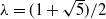 $\lambda =(1+\sqrt {5})/2$
. We represent two snapshots using dark blue (
$\lambda =(1+\sqrt {5})/2$
. We represent two snapshots using dark blue (
 $t=800$
) and yellow (
$t=800$
) and yellow (
 $t=1000$
). The star represents the constant-in-time solutions. Here, we note that not only diffusion rates, but other parameters as well, may affect the crime landscape. We observe that the magnitude and sign of
$t=1000$
). The star represents the constant-in-time solutions. Here, we note that not only diffusion rates, but other parameters as well, may affect the crime landscape. We observe that the magnitude and sign of
 $\chi$
can significantly impact the local density of both agents, leading to values far from the constant steady state.
$\chi$
can significantly impact the local density of both agents, leading to values far from the constant steady state.

However, as shown by the linear stability analysis in [Reference Yerlanov, Wang and Rodríguez62], no value of
 $D_u$
with fixed
$D_u$
with fixed
 $\chi = 4$
can shift the system into the linearly stable regime; in other words, there does not exist
$\chi = 4$
can shift the system into the linearly stable regime; in other words, there does not exist
 $D_u \gt 0$
such that
$D_u \gt 0$
such that
 $\chi ^- \lt \chi \lt \chi ^+$
for the parameters given in the caption of Figure 9. In this setting, high police concentration in highly attractive regions prevents the system from reaching spatial uniformity, regardless of adjustments to patrolling (i.e., random movement). In particular, when police movement has no advection component, the system decouples:
$\chi ^- \lt \chi \lt \chi ^+$
for the parameters given in the caption of Figure 9. In this setting, high police concentration in highly attractive regions prevents the system from reaching spatial uniformity, regardless of adjustments to patrolling (i.e., random movement). In particular, when police movement has no advection component, the system decouples:
 $u$
converges to a constant steady state, while the remaining scalar fields develop spatially heterogeneous solutions. In this case, the model effectively reduces to a two-component system, which has already been extensively studied in the works referenced in the introduction.
$u$
converges to a constant steady state, while the remaining scalar fields develop spatially heterogeneous solutions. In this case, the model effectively reduces to a two-component system, which has already been extensively studied in the works referenced in the introduction.
In our simulations, off-hotspot policing is associated with higher crime density and lower police presence, whereas the opposite trend is observed under hotspot policing. For example, in the bottom-left corner of Figure 9, the crime density reaches
 $\approx 28.3$
, about 73 times higher than the constant steady-state value. While such disparities may resemble the heterogeneous distribution of crime in urban areas (cf, [Reference Thacher50]), we emphasize that these findings are model-based and hypothetical. Further empirical validation would be required before drawing any policy implications.
$\approx 28.3$
, about 73 times higher than the constant steady-state value. While such disparities may resemble the heterogeneous distribution of crime in urban areas (cf, [Reference Thacher50]), we emphasize that these findings are model-based and hypothetical. Further empirical validation would be required before drawing any policy implications.
6. Conclusion and brief discussions
We have contributed to the understanding of the pattern formation of a model of urban crime by demonstrating the existence and stability of a nonhomogeneous solution bifurcating from the constant steady state. The bifurcation parameter,
 $\chi$
, does not have any restrictions in terms of its sign and hence a bifurcating point is always defined. The corresponding spatially nonconstant solutions are almost always present, but they are not always stable. Our approach relies on connecting the central system with the negative Laplacian eigenvalue problem, introduced by Cantrell et al. [Reference Cantrell, Cosner and Manásevich8]. This is a powerful tool, as it does not involve the wavemode vector and thus does not explicitly depend on the dimension of the problem. We employed this method to investigate the Hopf bifurcation and obtained a similar result to that derived for the one-dimensional case [Reference Rodríguez, Wang and Zhang39]. One could further extend and show the stability of periodic solutions, but we expect the results to be similar to those in [Reference Rodríguez, Wang and Zhang39]. In addition, we run numerical simulations of system (E), which confirm the theoretical results by demonstrating the existence of orbits. Even when solutions are not periodic, they still may exhibit interesting patterns, whose geometry can be studied as a separate future project. From a theoretical perspective, a worthwhile direction is to analyse chaos, which is only evidenced numerically in this paper, more rigorously. From a practical standpoint, a deeper understanding of various parameter combinations and corresponding solution behaviours needs to be studied as part of a potential comprehensive research design (e.g., how police should move given the current state of the system).
$\chi$
, does not have any restrictions in terms of its sign and hence a bifurcating point is always defined. The corresponding spatially nonconstant solutions are almost always present, but they are not always stable. Our approach relies on connecting the central system with the negative Laplacian eigenvalue problem, introduced by Cantrell et al. [Reference Cantrell, Cosner and Manásevich8]. This is a powerful tool, as it does not involve the wavemode vector and thus does not explicitly depend on the dimension of the problem. We employed this method to investigate the Hopf bifurcation and obtained a similar result to that derived for the one-dimensional case [Reference Rodríguez, Wang and Zhang39]. One could further extend and show the stability of periodic solutions, but we expect the results to be similar to those in [Reference Rodríguez, Wang and Zhang39]. In addition, we run numerical simulations of system (E), which confirm the theoretical results by demonstrating the existence of orbits. Even when solutions are not periodic, they still may exhibit interesting patterns, whose geometry can be studied as a separate future project. From a theoretical perspective, a worthwhile direction is to analyse chaos, which is only evidenced numerically in this paper, more rigorously. From a practical standpoint, a deeper understanding of various parameter combinations and corresponding solution behaviours needs to be studied as part of a potential comprehensive research design (e.g., how police should move given the current state of the system).
As the work of Cantrell and collaborators [Reference Cantrell, Cosner and Manásevich8] complements the work by Short et al. [Reference Short, Bertozzi and Brantingham46], this work complements our previous finding in [Reference Yerlanov, Wang and Rodríguez62], by providing the relevant Theorems. Although the approaches are similar, we note a few differences between this paper and that of Cantrell et al. [Reference Cantrell, Cosner and Manásevich8]. We have fewer restrictions on the parameter space for the first Theorem, as the control parameter does not have to be positive. On the other hand, we needed to impose more conditions to guarantee stability, as it is “easier” for the relevant characteristic equation to have positive real parts. Cantrell et al. stated that the relevant eigenvalues are those that are sufficiently small. This does not appear to be the case for the extended model. We hypothesize that under suitable conditions, any eigenvalue of the negative Laplacian would be relevant. It would be of interest to find the equivalent but simpler assumptions in the theorems. The apparent difference lies in the addition of the third equation, and hence, the increase in dimension from a linear algebra perspective. This comes with challenges, such as dealing with an already non-trivial kernel, third-degree polynomials and more convoluted expressions involving additional parameters, among others. One of the goals of this paper is to demonstrate how to overcome these hindrances, particularly as the number of equations and/or dimensions increases. This is part of a larger effort to investigate pattern formation in the general Keller–Segel model, where analysis has mainly been conducted on systems of two equations. By increasing the model’s dimension, one may obtain a more precise picture, but also introduce new complexity. However, with this complexity, new mathematical endeavours and insights emerge, and the authors hope that this paper will serve as a call and a guide to contribute to the field of pattern formation.
Financial support
This work was partially funded by NSF-DMS-2042413 and AFOSR MURI FA9550-22-1-0380.
Competing interests
None.
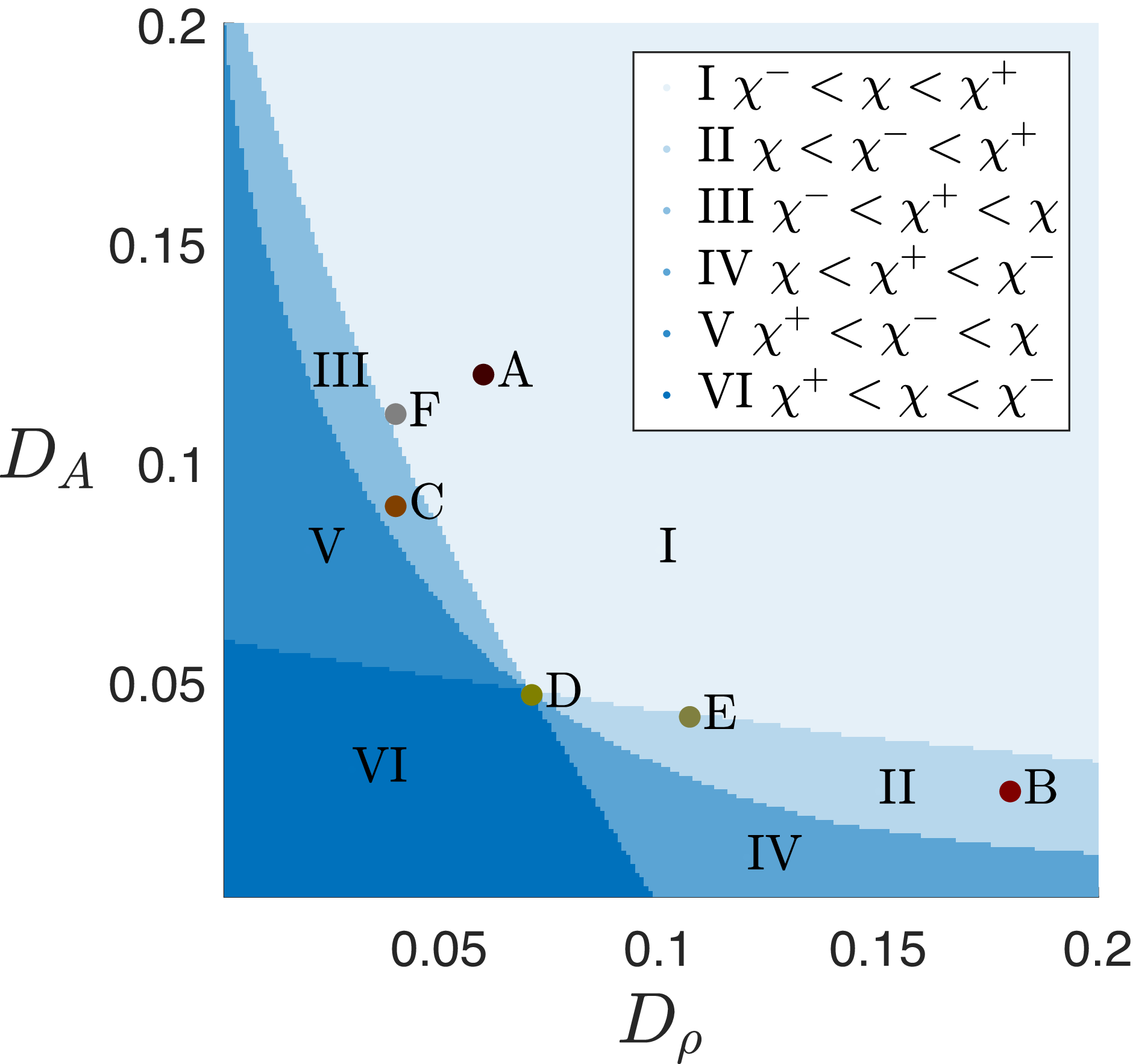


 Open access