


Impact Statement
This paper addresses the challenge of identifying intelligent sensor placements for monitoring environmental phenomena, using Antarctic air temperature anomaly as an example. The authors propose using a recent machine learning model—a convolutional Gaussian neural process (ConvGNP)—which can capture complex non-stationary behaviour and scale to large datasets. The ConvGNP outperforms previous data-driven approaches in simulated experiments, finding more informative and cost-effective sensor placements. This could lead to improved decision-making for monitoring weather conditions and climate change impacts.
1. Introduction
Selecting optimal locations for placing environmental sensors is an important scientific challenge. For example, improved environmental monitoring can lead to more accurate weather forecasting (Weissmann et al., Reference Weissmann, Harnisch, Wu, Lin, Ohta, Yamashita, Kim, Jeon, Nakazawa and Aberson2011; Jung et al., Reference Jung, Gordon, Bauer, Bromwich, Chevallier, Day, Dawson, Doblas-Reyes, Fairall, Goessling, Holland, Inoue, Iversen, Klebe, Lemke, Losch, Makshtas, Mills, Nurmi, Perovich, Reid, Renfrew, Smith, Svensson, Tolstykh and Yang2016). Further, better observation coverage can improve the representation of extreme events, climate variability, and long-term trends in reanalysis models (Bromwich and Fogt, Reference Bromwich and Fogt2004) and aid their validation (Bracegirdle and Marshall, Reference Bracegirdle and Marshall2012). This is particularly important in remote regions like Antarctica, where observations are sparse (Jung et al., Reference Jung, Gordon, Bauer, Bromwich, Chevallier, Day, Dawson, Doblas-Reyes, Fairall, Goessling, Holland, Inoue, Iversen, Klebe, Lemke, Losch, Makshtas, Mills, Nurmi, Perovich, Reid, Renfrew, Smith, Svensson, Tolstykh and Yang2016) and the cost of deploying weather stations is high (Lazzara et al., Reference Lazzara, Weidner, Keller, Thom and Cassano2012), motivating an objective model-based approach that provides an accurate notion of the informativeness of new observation locations. This informativeness can then guide decision-making so that scientific goals are achieved with as few sensors as possible.
The above sensor placement problem has been studied extensively from a physics-based numerical modelling perspective (Majumdar, Reference Majumdar2016). Multiple approaches exist for estimating the value of current or new observation locations for a numerical model. Examples include observing system simulation experiments (Hoffman and Atlas, Reference Hoffman and Atlas2016), adjoint methods (Langland and Baker, Reference Langland and Baker2004), and ensemble sensitivity analysis (ESA; Torn and Hakim, Reference Torn and Hakim2008). Using a numerical model for sensor placement comes with benefits and limitations. One drawback is that numerical models can be biased, and this can degrade sensor placements. This suggests that physics-based approaches could be supplemented by data-driven methods that learn statistical relationships directly from the data.
Machine learning (ML) methods also have a long history of use for experimental design and sensor placement (MacKay, Reference MacKay1992; Cohn, Reference Cohn1993; Seo et al., Reference Seo, Wallat, Graepel and Obermayer2000; Krause et al., Reference Krause, Singh and Guestrin2008). First, a probabilistic model is fit to noisy observations of an unknown function $ f\left(\boldsymbol{x}\right) $
. Then, active learning is used to identify new
$ f\left(\boldsymbol{x}\right) $
. Then, active learning is used to identify new $ \boldsymbol{x} $
-locations that are expected to maximally reduce the model’s uncertainty about some aspect of
$ \boldsymbol{x} $
-locations that are expected to maximally reduce the model’s uncertainty about some aspect of $ f\left(\boldsymbol{x}\right) $
. The Gaussian process (GP; Rasmussen, Reference Rasmussen2004) has so far been the go-to class of probabilistic model for sensor placement and the related task of Bayesian optimisationFootnote 1 (Singh et al., Reference Singh, Krause, Guestrin, Kaiser and Batalin2007; Krause et al., Reference Krause, Singh and Guestrin2008; Marchant and Ramos, Reference Marchant and Ramos2012; Shahriari et al., Reference Shahriari, Swersky, Wang, Adams and de Freitas2016). Setting up a GP requires the user to specify a mean function (describing the expected value of the function) and a covariance function (describing how correlated the
$ f\left(\boldsymbol{x}\right) $
. The Gaussian process (GP; Rasmussen, Reference Rasmussen2004) has so far been the go-to class of probabilistic model for sensor placement and the related task of Bayesian optimisationFootnote 1 (Singh et al., Reference Singh, Krause, Guestrin, Kaiser and Batalin2007; Krause et al., Reference Krause, Singh and Guestrin2008; Marchant and Ramos, Reference Marchant and Ramos2012; Shahriari et al., Reference Shahriari, Swersky, Wang, Adams and de Freitas2016). Setting up a GP requires the user to specify a mean function (describing the expected value of the function) and a covariance function (describing how correlated the $ f\left(\boldsymbol{x}\right) $
values are at different
$ f\left(\boldsymbol{x}\right) $
values are at different $ \boldsymbol{x} $
-locations). Once a GP has been initialised, conditioning it on observed data and evaluating at target locations produces a multivariate Gaussian distribution, which can be queried to search for informative sensor placements.
$ \boldsymbol{x} $
-locations). Once a GP has been initialised, conditioning it on observed data and evaluating at target locations produces a multivariate Gaussian distribution, which can be queried to search for informative sensor placements.
GPs have several compelling strengths which make them particularly amenable to small-data regimes and simple target functions. However, modelling a climate variable with a GP is challenging due to spatiotemporal non-stationarity and large volumes of data corresponding to multiple predictor variables. While non-stationary GP covariance functions are available (and improve sensor placement in Krause et al., Reference Krause, Singh and Guestrin2008 and Singh et al., Reference Singh, Ramos, Whyte and Kaiser2010), this still comes with the task of choosing the right functional form and introduces a risk of overfitting (Fortuin et al., Reference Fortuin, Strathmann and Rätsch2020). Further, conditioning GPs on supplementary predictor variables (such as satellite data) is non-trivial and their computational cost scales cubically with dataset size, which becomes prohibitive with large environmental datasets. Approximations allow GPs to scale to large data (Titsias, Reference Titsias2009; Hensman et al., Reference Hensman, Fusi and Lawrence2013), but these also harm prediction quality. The above model misspecifications can lead to uninformative or degraded sensor placements, motivating a new approach which can more faithfully capture the behaviour of complex environmental data.
Convolutional neural processes (ConvNPs) are a recent class of ML models that have shown promise in modelling environmental variables. For example, ConvNPs can outperform a large ensemble of climate downscaling approaches (Vaughan et al., Reference Vaughan, Tebbutt, Hosking and Turner2021; Markou et al., Reference Markou, Requeima, Bruinsma, Vaughan and Turner2022) and integrate data of gridded and point-based modalities (Bruinsma et al., Reference Bruinsma, Markou, Requeima, Foong, Andersson, Vaughan, Buonomo, Hosking and Turner2023). One variant, the convolutional Gaussian neural process (ConvGNP; Bruinsma et al., Reference Bruinsma, Requeima, Foong, Gordon and Turner2021; Markou et al., Reference Markou, Requeima, Bruinsma, Vaughan and Turner2022), uses neural networks to parameterise a joint Gaussian distribution at target locations, allowing them to scale linearly with dataset size while learning mean and covariance functions directly from the data.
In this paper, simulated atmospheric data is used to assess the ability of the ConvGNP to model a complex environmental variable and find informative sensor placements. The paper is laid out as follows. Section 2 introduces the data and describes the ConvGNP model. Section 3 compares the ConvGNP with GP baselines with three experiments: predicting unseen data, predicting the benefit of new observations, and a sensor placement toy experiment. It is then shown how placement informativeness can be traded-off with cost using multi-objective optimisation to enable a human-in-the-loop decision-support tool. Section 4 discusses limitations and possible extensions to our approach, contrasting ML-based and physics-based sensor placements. Concluding remarks are provided in Section 5.
2. Methods
In this section, we define the goal and data, formalise the problem tackled, and introduce the ConvGNP.
2.1. Goal and source data
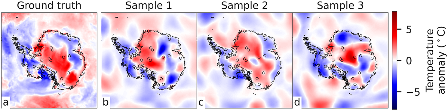
We use reanalysis data to analyse sensor placement abilities. Reanalysis data are produced by fitting a numerical climate model to observations using data assimilation (Gettelman et al., Reference Gettelman, Geer, Forbes, Carmichael, Feingold, Posselt, Stephens, van den Heever, Varble and Zuidema2022), capturing the complex dynamics of the Earth system on a regular grid. The simulated target variable used in this study is 25 km-resolution ERA5 daily-averaged 2 m temperature anomaly over Antarctica (Figure 2a; Hersbach et al., Reference Hersbach, Bell, Berrisford, Hirahara, Horányi, Muñoz-Sabater, Nicolas, Peubey, Radu, Schepers, Simmons, Soci, Abdalla, Abellan, Balsamo, Bechtold, Biavati, Bidlot, Bonavita, De Chiara, Dahlgren, Dee, Diamantakis, Dragani, Flemming, Forbes, Fuentes, Geer, Haimberger, Healy, Hogan, Hólm, Janisková, Keeley, Laloyaux, Lopez, Lupu, Radnoti, de Rosnay, Rozum, Vamborg, Villaume and Thépaut2020). For a given day of year, temperature anomalies are computed by subtracting maps of the mean daily temperature (averaged over 1950–2013) from the absolute temperature, removing the seasonal cycle. We train a ConvGNP and a set of GP baselines to produce probabilistic spatial interpolation predictions for ERA5 temperature anomalies, assessing performance on a range of metrics. We then perform simulated sensor placement experiments to quantitatively compare the ConvGNP’s estimates of observation informativeness with that of the GP baselines and simple heuristic placement methods. The locations of 79 Antarctic stations that recorded temperature on February 15, 2009 are used as the starting point for the sensor placement experiment (black crosses in Figure 1), simulating a realistic sensor network design scenario. Alongside inputs of ERA5 temperature anomaly observations, we also provide the ConvGNP with a second data stream on a 25 km grid, containing surface elevation and a land mask (obtained from the BedMachine dataset; Morlighem, Reference Morlighem2020), as well as space/time coordinate variables. For further details on the data sources and preprocessing see Supplementary Appendix A.
We have two context sets: ERA5 temperature anomaly observations and 6 gridded auxiliary fields, and we wish to make probabilistic predictions for temperature anomaly over a vertical line of target points (blue dotted line in left-most panel). In the ConvGNP, a SetConv layer fuses the context sets into a single gridded encoding (Supplementary Figure B1; Gordon et al., Reference Gordon, Bruinsma, Foong, Requeima, Dubois and Turner2020). A U-Net (Ronneberger et al., Reference Ronneberger, Fischer and Brox2015) takes this encoded tensor as input and outputs a gridded representation, which is interpolated at target points $ {\boldsymbol{X}}^{(t)} $
and used to parameterise the mean and covariance of a multivariate Gaussian distribution over
$ {\boldsymbol{X}}^{(t)} $
and used to parameterise the mean and covariance of a multivariate Gaussian distribution over $ {\boldsymbol{y}}^{(t)} $
. The output mean vector
$ {\boldsymbol{y}}^{(t)} $
. The output mean vector $ \boldsymbol{\mu} $
is shown as a black line, with 10 Gaussian samples overlaid in grey. The heatmap of the covariance matrix
$ \boldsymbol{\mu} $
is shown as a black line, with 10 Gaussian samples overlaid in grey. The heatmap of the covariance matrix $ \boldsymbol{K} $
shows the magnitude of spatial covariances, with covariance decreasing close to temperature anomaly context points.
$ \boldsymbol{K} $
shows the magnitude of spatial covariances, with covariance decreasing close to temperature anomaly context points.

(a) ERA5 2 m temperature anomaly on January 1, 2018; (b–d) ConvGNP samples with ERA5 temperature anomaly context points at Antarctic station locations (black circles). Comparing colours within the black circles across plots shows that the ConvGNP interpolates context observations.
2.2. Formal problem set-up
We now formalise the problem set-up tackled in this study. First, we make some simplifying assumptions about the data to be modelled. We assume that data from different time steps, $ \tau $
, are independent, and so we will not model temporal dependencies in the data. Further, we only consider variables that live in a 2D input space, as opposed to variables with a third input spatial dimension (e.g., altitude or depth). This simplifies the 3D or 4D modelling problem into a 2D one. Models built with these assumptions can learn correlations across 2D space, but not across time and/or height, which could be important in forecasting or oceanographic applications.
$ \tau $
, are independent, and so we will not model temporal dependencies in the data. Further, we only consider variables that live in a 2D input space, as opposed to variables with a third input spatial dimension (e.g., altitude or depth). This simplifies the 3D or 4D modelling problem into a 2D one. Models built with these assumptions can learn correlations across 2D space, but not across time and/or height, which could be important in forecasting or oceanographic applications.
At each $ \tau $
, there will be particular target locations
$ \tau $
, there will be particular target locations $ {\boldsymbol{X}}_{\tau}^{(t)}\in {\mathrm{\mathbb{R}}}^{N_t\times 2} $
where we wish to predict an environmental variable
$ {\boldsymbol{X}}_{\tau}^{(t)}\in {\mathrm{\mathbb{R}}}^{N_t\times 2} $
where we wish to predict an environmental variable $ {\boldsymbol{y}}_{\tau}^{(t)}\in {\mathrm{\mathbb{R}}}^{N_t} $
(we assume that the target variable is a 1D scalar for simplicity, but this need not be the case). Our target may be surface temperature anomaly along a line of points over Antarctica (blue dotted line in left-most panel of Figure 1). We call this a target set
$ {\boldsymbol{y}}_{\tau}^{(t)}\in {\mathrm{\mathbb{R}}}^{N_t} $
(we assume that the target variable is a 1D scalar for simplicity, but this need not be the case). Our target may be surface temperature anomaly along a line of points over Antarctica (blue dotted line in left-most panel of Figure 1). We call this a target set $ {T}_{\tau }=\left({\boldsymbol{X}}_{\tau}^{(t)},{\boldsymbol{y}}_{\tau}^{(t)}\right) $
. The target set predictions will be made using several data streams, containing
$ {T}_{\tau }=\left({\boldsymbol{X}}_{\tau}^{(t)},{\boldsymbol{y}}_{\tau}^{(t)}\right) $
. The target set predictions will be made using several data streams, containing $ N $
-D observations
$ N $
-D observations $ {\boldsymbol{Y}}_{\tau}^{(c)}\in {\mathrm{\mathbb{R}}}^{N_c\times N} $
at particular locations
$ {\boldsymbol{Y}}_{\tau}^{(c)}\in {\mathrm{\mathbb{R}}}^{N_c\times N} $
at particular locations $ {\boldsymbol{X}}_{\tau}^{(c)}\in {\mathrm{\mathbb{R}}}^{N_c\times 2} $
. We call these data streams context sets
$ {\boldsymbol{X}}_{\tau}^{(c)}\in {\mathrm{\mathbb{R}}}^{N_c\times 2} $
. We call these data streams context sets $ \left({\boldsymbol{X}}_{\tau}^{(c)},{\boldsymbol{Y}}_{\tau}^{(c)}\right) $
, and write the collection of all
$ \left({\boldsymbol{X}}_{\tau}^{(c)},{\boldsymbol{Y}}_{\tau}^{(c)}\right) $
, and write the collection of all $ {N}_C $
context sets as
$ {N}_C $
context sets as $ {C}_{\tau }={\left\{{\left({\boldsymbol{X}}_{\tau}^{(c)},{\boldsymbol{Y}}_{\tau}^{(c)}\right)}_i\right\}}_{i=1}^{N_C}. $
Context sets may lie on scattered, off-grid locations (e.g., temperature anomaly observations at black crosses in left-most panel in Figure 1) or on a regular grid (e.g., elevation and other auxiliary fields in the second panel of Figure 1). We call the collection of context sets and the target set a task
$ {C}_{\tau }={\left\{{\left({\boldsymbol{X}}_{\tau}^{(c)},{\boldsymbol{Y}}_{\tau}^{(c)}\right)}_i\right\}}_{i=1}^{N_C}. $
Context sets may lie on scattered, off-grid locations (e.g., temperature anomaly observations at black crosses in left-most panel in Figure 1) or on a regular grid (e.g., elevation and other auxiliary fields in the second panel of Figure 1). We call the collection of context sets and the target set a task $ {\mathcal{D}}_{\tau }=\left({C}_{\tau },{T}_{\tau}\right). $
The goal is to build an ML model that takes the context sets as input and maps to probabilistic predictions for the target values
$ {\mathcal{D}}_{\tau }=\left({C}_{\tau },{T}_{\tau}\right). $
The goal is to build an ML model that takes the context sets as input and maps to probabilistic predictions for the target values $ {\boldsymbol{y}}_{\tau}^{(t)} $
given the target locations
$ {\boldsymbol{y}}_{\tau}^{(t)} $
given the target locations $ {\boldsymbol{X}}_{\tau}^{(t)} $
. Following Foong et al., Reference Foong, Bruinsma, Gordon, Dubois, Requeima and Turner2020, we refer to this model as a prediction map,
$ {\boldsymbol{X}}_{\tau}^{(t)} $
. Following Foong et al., Reference Foong, Bruinsma, Gordon, Dubois, Requeima and Turner2020, we refer to this model as a prediction map, $ \pi $
. Once
$ \pi $
. Once $ \pi $
is set up, a sensor placement algorithm
$ \pi $
is set up, a sensor placement algorithm $ \mathcal{S} $
will use
$ \mathcal{S} $
will use $ \pi $
to propose
$ \pi $
to propose $ K $
new placement locations
$ K $
new placement locations $ {\boldsymbol{X}}^{\ast}\in {\mathrm{\mathbb{R}}}^{K\times 2} $
based on query locations
$ {\boldsymbol{X}}^{\ast}\in {\mathrm{\mathbb{R}}}^{K\times 2} $
based on query locations $ {\boldsymbol{X}}^{(s)}\in {\mathrm{\mathbb{R}}}^{S\times 2} $
and a set of tasks
$ {\boldsymbol{X}}^{(s)}\in {\mathrm{\mathbb{R}}}^{S\times 2} $
and a set of tasks $ {\left\{{\mathcal{D}}_{\tau_j}\right\}}_{j=1}^J $
. Section 3.2 provides details on how we implement
$ {\left\{{\mathcal{D}}_{\tau_j}\right\}}_{j=1}^J $
. Section 3.2 provides details on how we implement $ \mathcal{S} $
in practice.
$ \mathcal{S} $
in practice.
Physics-based numerical models could be framed as hard-coded prediction maps, ingesting context sets through data assimilation schemes and using physical laws to predict targets on a regular grid over space and time. These model outputs are deterministic by default, but applying stochastic perturbations to initial conditions or model parameters induces an intractable distribution over model outputs, $ p\left({\boldsymbol{y}}^{(t)}\right) $
, which can be sampled from to generate an ensemble of reanalyses or forecasts. However, current numerical models do not learn directly from data. In contrast, ML-based prediction maps will be trained from scratch to directly output a distribution over targets based on the context data.
$ p\left({\boldsymbol{y}}^{(t)}\right) $
, which can be sampled from to generate an ensemble of reanalyses or forecasts. However, current numerical models do not learn directly from data. In contrast, ML-based prediction maps will be trained from scratch to directly output a distribution over targets based on the context data.
2.3. ConvGNP model
Most ML methods are ill-suited to the problem described in Section 2.2. Typical deep learning approaches used in environmental applications, such as convolutional neural networks, require the data to lie on a regular grid, and thus cannot handle non-gridded data (e.g., Andersson et al., Reference Andersson, Hosking, Pérez-Ortiz, Paige, Elliott, Russell, Law, Jones, Wilkinson, Phillips, Byrne, Tietsche, Sarojini, Blanchard-Wrigglesworth, Aksenov, Downie and Shuckburgh2021; Ravuri et al., Reference Ravuri, Lenc, Willson, Kangin, Lam, Mirowski, Fitzsimons, Athanassiadou, Kashem, Madge, Prudden, Mandhane, Clark, Brock, Simonyan, Hadsell, Robinson, Clancy, Arribas and Mohamed2021). Recent emerging architectures such as transformers can handle off-the-grid data in principle, but in practice have used gridded data in environmental applications (e.g., Bi et al., Reference Bi, Xie, Zhang, Chen, Gu and Tian2022). Moreover, they also need architectural changes to make predictions at previously unseen input locations. On the other hand, Bayesian probabilistic models based on stochastic processes (such as GPs) can ingest data at arbitrary locations, but it is difficult to integrate more than one input data stream, especially when those streams are high dimensional (e.g., supplementary satellite data which aids the prediction task). Neural processes (NPs; Garnelo et al., Reference Garnelo, Rosenbaum, Maddison, Ramalho, Saxton, Shanahan, Teh, Rezende and Eslami2018a, Reference Garnelo, Schwarz, Rosenbaum, Viola, Rezende, Eslami and Teh2018b) are prediction maps that address these problems by combining the modelling flexibility and scalability of neural networks with the uncertainty quantification benefits of GPs. The ConvGNP is a particular prediction map $ \pi $
whose output distribution is a correlated (joint) Gaussian with mean
$ \pi $
whose output distribution is a correlated (joint) Gaussian with mean $ \boldsymbol{\mu} $
and covariance matrix
$ \boldsymbol{\mu} $
and covariance matrix $ \boldsymbol{K} $
:
$ \boldsymbol{K} $
:
 $$ \pi \left({\boldsymbol{y}}^{(t)};C,{\boldsymbol{X}}^{(t)}\right)=\mathcal{N}\left({\boldsymbol{y}}^{(t)};\boldsymbol{\mu} \left(C,{\boldsymbol{X}}^{(t)}\right),\boldsymbol{K}\hskip-0.35em \left(C,{\boldsymbol{X}}^{(t)}\right)\right). $$
The ConvGNP takes in the context sets $ C $
and outputs a mean and non-stationary covariance function of a GP predictive, which can be queried at arbitrary target locations (Figure 1). It does this by first fusing the context sets into a gridded encoding using a SetConv layer (Gordon et al., Reference Gordon, Bruinsma, Foong, Requeima, Dubois and Turner2020). The SetConv encoder interpolates context observations onto an internal grid with the density of observations captured by a “density channel” for each context set (example encoding shown in Supplementary Figure B1). This endows the model with the ability to ingest multiple predictors of various modalities (gridded and point-based) and handle missing data (Supplementary Appendix B.5). The gridded encoding is passed to a U-Net (Ronneberger et al., Reference Ronneberger, Fischer and Brox2015), which produces a representation of the context sets with
$ C $
and outputs a mean and non-stationary covariance function of a GP predictive, which can be queried at arbitrary target locations (Figure 1). It does this by first fusing the context sets into a gridded encoding using a SetConv layer (Gordon et al., Reference Gordon, Bruinsma, Foong, Requeima, Dubois and Turner2020). The SetConv encoder interpolates context observations onto an internal grid with the density of observations captured by a “density channel” for each context set (example encoding shown in Supplementary Figure B1). This endows the model with the ability to ingest multiple predictors of various modalities (gridded and point-based) and handle missing data (Supplementary Appendix B.5). The gridded encoding is passed to a U-Net (Ronneberger et al., Reference Ronneberger, Fischer and Brox2015), which produces a representation of the context sets with $ \boldsymbol{R}=\mathrm{U}\mathrm{N}\mathrm{e}\mathrm{t}(\mathrm{S}\mathrm{e}\mathrm{t}\mathrm{C}\mathrm{o}\mathrm{n}\mathrm{v}(C)) $
. The tensor
$ \boldsymbol{R}=\mathrm{U}\mathrm{N}\mathrm{e}\mathrm{t}(\mathrm{S}\mathrm{e}\mathrm{t}\mathrm{C}\mathrm{o}\mathrm{n}\mathrm{v}(C)) $
. The tensor $ \boldsymbol{R} $
is then spatially interpolated at each target location
$ \boldsymbol{R} $
is then spatially interpolated at each target location $ {\boldsymbol{x}}_i^{(t)} $
, yielding a vector
$ {\boldsymbol{x}}_i^{(t)} $
, yielding a vector $ {\boldsymbol{r}}_i $
and enabling the model to predict at arbitrary locations. Finally,
$ {\boldsymbol{r}}_i $
and enabling the model to predict at arbitrary locations. Finally, $ {\boldsymbol{r}}_i $
is passed to multilayer perceptrons
$ {\boldsymbol{r}}_i $
is passed to multilayer perceptrons $ f $
and
$ f $
and $ \boldsymbol{g} $
, parameterising the mean and covariance respectively with
$ \boldsymbol{g} $
, parameterising the mean and covariance respectively with $ {\mu}_i=f\left({\boldsymbol{r}}_i\right) $
and
$ {\mu}_i=f\left({\boldsymbol{r}}_i\right) $
and $ {k}_{ij}=\boldsymbol{g}{\left({\boldsymbol{r}}_i\right)}^T\boldsymbol{g}\left({\boldsymbol{r}}_j\right) $
. This architecture results in a mean vector
$ {k}_{ij}=\boldsymbol{g}{\left({\boldsymbol{r}}_i\right)}^T\boldsymbol{g}\left({\boldsymbol{r}}_j\right) $
. This architecture results in a mean vector $ \boldsymbol{\mu} $
and covariance matrix
$ \boldsymbol{\mu} $
and covariance matrix $ \boldsymbol{K} $
that are functions of
$ \boldsymbol{K} $
that are functions of $ C $
and
$ C $
and $ {\boldsymbol{X}}^{(t)} $
(Equation 1).
$ {\boldsymbol{X}}^{(t)} $
(Equation 1).
Constructing the covariances via a dot product leads to a low-rank covariance matrix structure, which is exploited to reduce the computational cost of predictions from cubic to linear in the number of targets. Furthermore, the use of a SetConv to encode the context sets results in linear scaling with the number of context points. This out-of-the-box scalability allows the ConvGNP to process 100,000 context points and predict over 100,000 target points in less than a second on a single GPU.Footnote 2
NPs can be considered meta-learning models (Foong et al., Reference Foong, Bruinsma, Gordon, Dubois, Requeima and Turner2020) which learn how to learn, mapping directly from context sets to predictions without requiring retraining when presented with new tasks. This is useful in environmental sciences because it enables learning statistical relationships (such as correlations) that depend on the context observations. In contrast, conventional supervised learning models, such as GPs, instead learn fixed statistical relationships which do not depend on the context observations.
2.4. Training the ConvGNP
Training tasks $ {\mathcal{D}}_{\tau } $
are generated by first sampling the day
$ {\mathcal{D}}_{\tau } $
are generated by first sampling the day $ \tau $
randomly from the training period, 1950–2013. Then, ERA5 grid cells are sampled uniformly at random across the entire 280 × 280 input space, with the number of ERA5 temperature anomaly context and target points drawn uniformly at random from
$ \tau $
randomly from the training period, 1950–2013. Then, ERA5 grid cells are sampled uniformly at random across the entire 280 × 280 input space, with the number of ERA5 temperature anomaly context and target points drawn uniformly at random from $ {N}_c\in \left\{5,6,\dots, 500\right\} $
and
$ {N}_c\in \left\{5,6,\dots, 500\right\} $
and $ {N}_t\in \{3000,3001,\dots, 4000\} $
. The ConvGNP is trained to minimise the negative log-likelihood (NLL) of target values
$ {N}_t\in \{3000,3001,\dots, 4000\} $
. The ConvGNP is trained to minimise the negative log-likelihood (NLL) of target values $ {\boldsymbol{y}}_{\tau}^{(t)} $
under its output Gaussian distribution using the Adam optimiser. After each training epoch, the model is checkpointed if an improvement is made to the mean NLL on validation tasks from 2014 to 2017. For further model and training details see Supplementary Appendix B.
$ {\boldsymbol{y}}_{\tau}^{(t)} $
under its output Gaussian distribution using the Adam optimiser. After each training epoch, the model is checkpointed if an improvement is made to the mean NLL on validation tasks from 2014 to 2017. For further model and training details see Supplementary Appendix B.
Once trained in this manner, the ConvGNP outputs expressive, non-stationary mean and covariance functions. When conditioning the ConvGNP on ERA5 temperature anomaly observations and drawing Gaussian samples on a regular grid, the samples interpolate observations at the context points and extrapolate plausible scenarios away from them (Figure 2). Running the ConvGNP on a regular grid with no temperature anomaly observations reveals the prior covariance structure learned by the model (Figure 3). The ConvGNP leverages the gridded auxiliary fields and day of year inputs from the second context set to output highly non-stationary spatial dependencies in surface temperature, such as sharp drops in covariance over the coastline (Figure 3a–c), anticorrelation (Figure 3a), and decorrelation over the Transantarctic Mountains (Figure 3b). In Supplementary Appendix D, we contrast this with GP prior covariances and further show that the ConvGNP learns seasonally varying spatial correlation (Supplementary Figures D1–D3).
Prior covariance function, $ k\left({\boldsymbol{x}}_1,{\boldsymbol{x}}_2\right) $
, with
$ k\left({\boldsymbol{x}}_1,{\boldsymbol{x}}_2\right) $
, with $ {\boldsymbol{x}}_1 $
fixed at the white plus location and
$ {\boldsymbol{x}}_1 $
fixed at the white plus location and $ {\boldsymbol{x}}_2 $
varying over the grid. Plots are shown for three different
$ {\boldsymbol{x}}_2 $
varying over the grid. Plots are shown for three different $ {\boldsymbol{x}}_1 $
-locations (the Ross Ice Shelf, the South Pole, and East Antarctica) for the 1st of June. The most prominent section of the Transantarctic Mountains is indicated by the red dashed line in (b).
$ {\boldsymbol{x}}_1 $
-locations (the Ross Ice Shelf, the South Pole, and East Antarctica) for the 1st of June. The most prominent section of the Transantarctic Mountains is indicated by the red dashed line in (b).

3. Results
We evaluate the ConvGNP’s ability to model ERA5 2 m daily-average surface temperature anomaly through a range of experiments, using GP baselines with both non-stationary and stationary covariance functions. We use three GP baselines with different non-isotropic covariance functions: the exponentiated quadratic (EQ), the rational quadratic (RQ), and the Gibbs kernel. The EQ and RQ are stationary because the covariance depends only on the difference between two input points, $ k\left(\boldsymbol{x},{\boldsymbol{x}}^{\prime}\right)=k\left(\boldsymbol{x}-{\boldsymbol{x}}^{\prime}\right) $
. The Gibbs covariance function is a more sophisticated, non-stationary baseline, where the correlation length scale is allowed to vary over space (Supplementary Figure C1). As noted in Section 2.3, there is no simple way to condition vanilla GP models on multiple context sets; the GP baselines can only ingest the context set containing the ERA5 observations and not the second, auxiliary context set. For more details on the GPs, including their covariance functions and training procedure, see Supplementary Appendix C.
$ k\left(\boldsymbol{x},{\boldsymbol{x}}^{\prime}\right)=k\left(\boldsymbol{x}-{\boldsymbol{x}}^{\prime}\right) $
. The Gibbs covariance function is a more sophisticated, non-stationary baseline, where the correlation length scale is allowed to vary over space (Supplementary Figure C1). As noted in Section 2.3, there is no simple way to condition vanilla GP models on multiple context sets; the GP baselines can only ingest the context set containing the ERA5 observations and not the second, auxiliary context set. For more details on the GPs, including their covariance functions and training procedure, see Supplementary Appendix C.
3.1. Performance on unseen data
To assess the models’ abilities to predict unseen data, 30,618 tasks are generated from unseen test years 2018–2019 by sampling ERA5 grid cells uniformly at random with number of targets $ {N}_t=\mathrm{2,000} $
and a range of context set sizes
$ {N}_t=\mathrm{2,000} $
and a range of context set sizes $ {N}_c\in \left\{\mathrm{0,25,50},\dots, 500\right\} $
(Supplementary Appendix B.1). For each task, we compute three performance metrics of increasing complexity. The first metric, the root mean squared error (RMSE), simply measures the difference between the model’s mean prediction and the true values. The second metric, the mean marginal NLL, includes the variances of the model’s point-wise Gaussian distributions, measuring how confident and well-calibrated the marginal distributions are. The third metric, the joint NLL, uses the model’s full joint Gaussian distribution, measuring how likely the true
$ {N}_c\in \left\{\mathrm{0,25,50},\dots, 500\right\} $
(Supplementary Appendix B.1). For each task, we compute three performance metrics of increasing complexity. The first metric, the root mean squared error (RMSE), simply measures the difference between the model’s mean prediction and the true values. The second metric, the mean marginal NLL, includes the variances of the model’s point-wise Gaussian distributions, measuring how confident and well-calibrated the marginal distributions are. The third metric, the joint NLL, uses the model’s full joint Gaussian distribution, measuring how likely the true $ {\boldsymbol{y}}^{(t)} $
vector is under the model. This quantifies the reliability of the model’s off-diagonal spatial correlations as well as its marginal variances.
$ {\boldsymbol{y}}^{(t)} $
vector is under the model. This quantifies the reliability of the model’s off-diagonal spatial correlations as well as its marginal variances.
In general, the ConvGNP performs best, followed by the Gibbs GP, the RQ GP, and finally the EQ GP (Figure 4). There are some exceptions to this trend. For example, the models produce similar RMSEs for $ {N}_c<100 $
. This is likely because for small
$ {N}_c<100 $
. This is likely because for small $ {N}_c $
the models revert to zero-mean predictions away from context points (matching the zero-mean of temperature anomaly over the training period). Another exception is that the Gibbs GP outperforms the ConvGNP on joint NLL for small
$ {N}_c $
the models revert to zero-mean predictions away from context points (matching the zero-mean of temperature anomaly over the training period). Another exception is that the Gibbs GP outperforms the ConvGNP on joint NLL for small $ {N}_c $
. This may be because the ConvGNP’s training process biases learning towards “easier” tasks (where
$ {N}_c $
. This may be because the ConvGNP’s training process biases learning towards “easier” tasks (where $ {N}_c $
is larger). Alternatively, the ConvGNP’s low-rank covariance parameterisation could be poorly suited to small
$ {N}_c $
is larger). Alternatively, the ConvGNP’s low-rank covariance parameterisation could be poorly suited to small $ {N}_c $
. However, with increasing
$ {N}_c $
. However, with increasing $ {N}_c $
, the ConvGNP significantly outperforms all three GP baselines across all three metrics, with its performance improving at a faster rate with added data. When averaging the results across
$ {N}_c $
, the ConvGNP significantly outperforms all three GP baselines across all three metrics, with its performance improving at a faster rate with added data. When averaging the results across $ {N}_c $
, the ConvGNP significantly outperforms all three GP baselines for each metric (Supplementary Table E1). We further find that the ConvGNP’s marginal distributions are substantially sharper and better calibrated than the GP baselines (Supplementary Figures E1 and E2), which is an important goal for probabilistic models (Gneiting et al., Reference Gneiting, Balabdaoui and Raftery2007). Well-calibrated uncertainties are also key for active learning, which is explored below in Section 3.2.
$ {N}_c $
, the ConvGNP significantly outperforms all three GP baselines for each metric (Supplementary Table E1). We further find that the ConvGNP’s marginal distributions are substantially sharper and better calibrated than the GP baselines (Supplementary Figures E1 and E2), which is an important goal for probabilistic models (Gneiting et al., Reference Gneiting, Balabdaoui and Raftery2007). Well-calibrated uncertainties are also key for active learning, which is explored below in Section 3.2.
Mean metric values versus number of context points on the test set. The joint negative log-likelihood (NLL) is normalised by the number of targets. Error bars are standard errors.

3.2. Sensor placement
Following previous works (Krause et al., Reference Krause, Singh and Guestrin2008), we pose sensor placement as a discrete optimisation problem. The task is to propose a subset of $ K $
sensor placement locations,
$ K $
sensor placement locations, $ {\boldsymbol{X}}^{\ast } $
, from a set of
$ {\boldsymbol{X}}^{\ast } $
, from a set of $ S $
search locations,
$ S $
search locations, $ {\boldsymbol{X}}^{(s)} $
. In practice, to avoid the infeasible combinatorial cost of searching over multiple placements jointly, a greedy approximation is made by selecting one sensor placement at a time. Within a greedy iteration, a value is assigned to each query location
$ {\boldsymbol{X}}^{(s)} $
. In practice, to avoid the infeasible combinatorial cost of searching over multiple placements jointly, a greedy approximation is made by selecting one sensor placement at a time. Within a greedy iteration, a value is assigned to each query location $ {\boldsymbol{x}}_i^{(s)} $
using an acquisition function,
$ {\boldsymbol{x}}_i^{(s)} $
using an acquisition function, $ \alpha \left({\boldsymbol{x}}_i^{(s)},\tau \right) $
, specifying the utility of a new observation at
$ \alpha \left({\boldsymbol{x}}_i^{(s)},\tau \right) $
, specifying the utility of a new observation at $ {\boldsymbol{x}}_i^{(s)} $
for time
$ {\boldsymbol{x}}_i^{(s)} $
for time $ \tau $
, which we average over
$ \tau $
, which we average over $ J $
dates:
$ J $
dates:
 $$ \alpha \left({\boldsymbol{x}}_i^{(s)}\right)=\frac{1}{J}\sum \limits_{j=1}^J\alpha \left({\boldsymbol{x}}_i^{(s)},{\tau}_j\right). $$
We use five acquisition functions which are to be maximised, defining a set of placement criteria (mathematical definitions are provided in Supplementary Appendix F):
JointMI: mutual information (MI) between the model’s prediction and the query sensor observation, imputing the missing value with the model’s mean at the query location, $ {\overline{y}}_{\tau, i}^{(s)} $
.Footnote 3 This criterion attempts to minimise the model’s joint entropy by minimising the log-determinant of the output covariance matrix, balancing minimising marginal variances with maximising correlation magnitude, which can be viewed as minimising uncertainty about the spatial patterns (MacKay, Reference MacKay1992). The joint MI has been used frequently in past work (Lindley, Reference Lindley1956; Krause et al., Reference Krause, Singh and Guestrin2008; Schmidt et al., Reference Schmidt, Smith, Hite, Mattingly, Azmy, Rajan and Goldhahn2019).
$ {\overline{y}}_{\tau, i}^{(s)} $
.Footnote 3 This criterion attempts to minimise the model’s joint entropy by minimising the log-determinant of the output covariance matrix, balancing minimising marginal variances with maximising correlation magnitude, which can be viewed as minimising uncertainty about the spatial patterns (MacKay, Reference MacKay1992). The joint MI has been used frequently in past work (Lindley, Reference Lindley1956; Krause et al., Reference Krause, Singh and Guestrin2008; Schmidt et al., Reference Schmidt, Smith, Hite, Mattingly, Azmy, Rajan and Goldhahn2019).
MarginalMI: as above, but ignoring the off-diagonal elements in the models’ Gaussian distributions and considering only the diagonal (marginal) entries. This criterion attempts to minimise the model’s marginal entropy by minimising the log variances in the output distribution.
DeltaVar: decrease in average marginal variance in the output distribution (similar to MarginalMI but using absolute variances rather than log-variances). Previous works have used this criterion for active learning both with neural networks (Cohn, Reference Cohn1993) and GPs (Seo et al., Reference Seo, Wallat, Graepel and Obermayer2000).
ContextDist: distance to the closest sensor. This is a simple heuristic which proposes placements as far away as possible from the current observations. While this is a strong baseline, non-stationarities in the data will mean that it is sub-optimal. For example, a high density of sensors will be needed in areas where correlation length scales are short, and a low density where they are large. Therefore, the optimal sensor placement strategy should differ from and outperform this approach.
Random: uniform white noise function (i.e., placing sensors randomly). The performance of this criterion reflects the average benefit of adding new observations for a given model and context set.
The target locations $ {\boldsymbol{X}}_{\tau}^{(t)} $
and search locations
$ {\boldsymbol{X}}_{\tau}^{(t)} $
and search locations $ {\boldsymbol{X}}^{(s)} $
are both defined on a 100 km grid over Antarctica, resulting in
$ {\boldsymbol{X}}^{(s)} $
are both defined on a 100 km grid over Antarctica, resulting in $ {N}_t=S=\mathrm{1,365} $
targets and possible placement locations. The context set locations
$ {N}_t=S=\mathrm{1,365} $
targets and possible placement locations. The context set locations $ {\boldsymbol{X}}_{\tau}^{(c)} $
are fixed at Antarctic temperature station locations (black circles in Figure 5) to simulate a realistic network design scenario. We use
$ {\boldsymbol{X}}_{\tau}^{(c)} $
are fixed at Antarctic temperature station locations (black circles in Figure 5) to simulate a realistic network design scenario. We use $ J=105 $
dates from the validation period (2014–2017), sampled at a 14-day interval, to compute the acquisition functions. Heatmaps showing the above five acquisition functions on the
$ J=105 $
dates from the validation period (2014–2017), sampled at a 14-day interval, to compute the acquisition functions. Heatmaps showing the above five acquisition functions on the $ {\boldsymbol{X}}^{(s)} $
grid, using the ConvGNP for the model underlying the three uncertainty-reduction acquisition functions, are shown in Figure 5. There are interesting differences between the model-based acquisition functions of the ConvGNP, the Gibbs GP, and the EQ GP (Supplementary Figure F1).
$ {\boldsymbol{X}}^{(s)} $
grid, using the ConvGNP for the model underlying the three uncertainty-reduction acquisition functions, are shown in Figure 5. There are interesting differences between the model-based acquisition functions of the ConvGNP, the Gibbs GP, and the EQ GP (Supplementary Figure F1).
Maps of acquisition function values $ \alpha \left({\boldsymbol{x}}_i^{(s)}\right) $
for the initial
$ \alpha \left({\boldsymbol{x}}_i^{(s)}\right) $
for the initial $ k=1 $
greedy iteration. The initial context set
$ k=1 $
greedy iteration. The initial context set $ {\boldsymbol{X}}^{(c)} $
is derived from real Antarctic station locations (black circles). Running the sensor placement algorithm for
$ {\boldsymbol{X}}^{(c)} $
is derived from real Antarctic station locations (black circles). Running the sensor placement algorithm for $ K=10 $
sensor placements results in the proposed sensor placements
$ K=10 $
sensor placements results in the proposed sensor placements $ {\boldsymbol{X}}^{\ast } $
(white pluses). Each pixel is
$ {\boldsymbol{X}}^{\ast } $
(white pluses). Each pixel is $ 100\times $ $ 100 $
km.
$ 100 $
km.

3.2.1. Oracle acquisition function experiment
By using sensor placement criteria that reduce uncertainty in the model’s predictions, one hopes that predictions also become more accurate in some way. For example, the entropy of the model’s predictive distribution is the expected NLL of the data under the model, so the decrease in entropy from a new observation (i.e., the MI) should relate to the NLL improvement—assuming the model is well-specified for the data. Further, if the model’s marginal distributions are well-calibrated, marginal variance relates to expected squared error. Therefore, the JointMI, MarginalMI, and DeltaVar acquisition functions should relate to improvements in joint NLL, marginal NLL, and RMSE, respectively. However, in general, the strength of these relationships are unknown. In the toy setting of this study, where ERA5 is treated as ground truth and is known everywhere, these relationships can be examined empirically.
We compare the ability of the ConvGNP, Gibbs GP, and EQ GP to predict the benefit of new observations based on the JointMI, MarginalMI, and DeltaVar acquisition functions, using ContextDist as a naïve baseline. The true benefit of observations is determined using oracle acquisition functions, $ {\alpha}_{\mathrm{oracle}} $
, where the true ERA5 value is revealed at
$ {\alpha}_{\mathrm{oracle}} $
, where the true ERA5 value is revealed at $ {\boldsymbol{x}}_i^{(s)} $
and the average performance gain on the target set is measured for each metric: joint NLL, marginal NLL, and RMSE (Supplementary Appendix F.3). Computing non-oracle and oracle acquisition functions at all
$ {\boldsymbol{x}}_i^{(s)} $
and the average performance gain on the target set is measured for each metric: joint NLL, marginal NLL, and RMSE (Supplementary Appendix F.3). Computing non-oracle and oracle acquisition functions at all $ S $
query locations produces vectors,
$ S $
query locations produces vectors, $ \boldsymbol{\alpha} \left({\boldsymbol{X}}^{(s)}\right) $
and
$ \boldsymbol{\alpha} \left({\boldsymbol{X}}^{(s)}\right) $
and $ {\boldsymbol{\alpha}}_{\mathrm{oracle}}\left({\boldsymbol{X}}^{(s)}\right) $
. The Pearson correlation
$ {\boldsymbol{\alpha}}_{\mathrm{oracle}}\left({\boldsymbol{X}}^{(s)}\right) $
. The Pearson correlation $ r=\mathrm{c}\mathrm{o}\mathrm{r}\mathrm{r}(\boldsymbol{\alpha} ({\boldsymbol{X}}^{(s)}),{\boldsymbol{\alpha}}_{\mathrm{oracle}}({\boldsymbol{X}}^{(s)})) $
between these vectors quantifies how strong the relationship is for a given model, acquisition function, and metric. With the context set initialised at Antarctic station locations (Section 3.2), the ConvGNP’s joint MI achieves the best correlation with its joint NLL improvement (
$ r=\mathrm{c}\mathrm{o}\mathrm{r}\mathrm{r}(\boldsymbol{\alpha} ({\boldsymbol{X}}^{(s)}),{\boldsymbol{\alpha}}_{\mathrm{oracle}}({\boldsymbol{X}}^{(s)})) $
between these vectors quantifies how strong the relationship is for a given model, acquisition function, and metric. With the context set initialised at Antarctic station locations (Section 3.2), the ConvGNP’s joint MI achieves the best correlation with its joint NLL improvement ( $ r=0.90 $
), as for its marginal MI with its marginal NLL improvement (
$ r=0.90 $
), as for its marginal MI with its marginal NLL improvement ( $ r=0.93 $
) and its change in variance with its RMSE improvement (
$ r=0.93 $
) and its change in variance with its RMSE improvement ( $ r=0.93 $
) (Figure 6a), substantially outperforming the ContextDist baseline in each case. The Gibbs GP’s acquisition functions are less robust at predicting performance gain, with the joint MI being particularly poor at predicting joint NLL improvement (Figure 6b). The EQ GP’s model-based acquisition functions all perform similarly to ContextDist for each metric (Figure 6c), which is likely an artefact of its stationary covariance function.
$ r=0.93 $
) (Figure 6a), substantially outperforming the ContextDist baseline in each case. The Gibbs GP’s acquisition functions are less robust at predicting performance gain, with the joint MI being particularly poor at predicting joint NLL improvement (Figure 6b). The EQ GP’s model-based acquisition functions all perform similarly to ContextDist for each metric (Figure 6c), which is likely an artefact of its stationary covariance function.
Correlation between model-based and oracle acquisition functions, $ \boldsymbol{\alpha} \left({\boldsymbol{X}}^{(s)}\right) $
and
$ \boldsymbol{\alpha} \left({\boldsymbol{X}}^{(s)}\right) $
and $ {\boldsymbol{\alpha}}_{\mathrm{oracle}}\left({\boldsymbol{X}}^{(s)}\right) $
. Error bars indicate the 2.5–97.5% quantiles from 5,000 bootstrapped correlation values, computed by resampling the 1,365 pairs of points with replacement, measuring how spatially consistent the correlation is across the search space
$ {\boldsymbol{\alpha}}_{\mathrm{oracle}}\left({\boldsymbol{X}}^{(s)}\right) $
. Error bars indicate the 2.5–97.5% quantiles from 5,000 bootstrapped correlation values, computed by resampling the 1,365 pairs of points with replacement, measuring how spatially consistent the correlation is across the search space $ {\boldsymbol{X}}^{(s)} $
.
$ {\boldsymbol{X}}^{(s)} $
.

We repeat the above analysis using the Kendall rank correlation coefficient, $ \kappa $
, which measures the similarity between the rankings of
$ \kappa $
, which measures the similarity between the rankings of $ \boldsymbol{\alpha} $
and
$ \boldsymbol{\alpha} $
and $ {\boldsymbol{\alpha}}_{\mathrm{oracle}} $
by computing the fraction of all pairs of search points
$ {\boldsymbol{\alpha}}_{\mathrm{oracle}} $
by computing the fraction of all pairs of search points $ \left({\boldsymbol{x}}_i^{(s)},{\boldsymbol{x}}_j^{(s)}\right) $
that are ordered the same way in the two rankings and normalising this fraction to lie in
$ \left({\boldsymbol{x}}_i^{(s)},{\boldsymbol{x}}_j^{(s)}\right) $
that are ordered the same way in the two rankings and normalising this fraction to lie in $ \left(-1,1\right) $
(Supplementary equation G.3). The findings are very similar to the Pearson correlation results above: only the ConvGNP has good alignment between acquisition functions and metrics, with JointMI, MarginalMI, and DeltaVar obtaining the best
$ \left(-1,1\right) $
(Supplementary equation G.3). The findings are very similar to the Pearson correlation results above: only the ConvGNP has good alignment between acquisition functions and metrics, with JointMI, MarginalMI, and DeltaVar obtaining the best $ \kappa $
-values for joint NLL (
$ \kappa $
-values for joint NLL ( $ \kappa =0.74 $
), marginal NLL (
$ \kappa =0.74 $
), marginal NLL ( $ \kappa =0.82 $
), and RMSE (
$ \kappa =0.82 $
), and RMSE ( $ \kappa =0.84 $
), respectively (Supplementary Figure G1).
$ \kappa =0.84 $
), respectively (Supplementary Figure G1).
These results indicate that the ConvGNP can robustly predict performance gain, unlike the GP baselines. Supplementary Appendix G provides more detailed plots from this experiment, including the acquisition function heatmaps (Supplementary Figures G2–G4) and scatter plots for all the oracle/non-oracle pairs underlying Figure 6 (Supplementary Figures G5–G7).
3.2.2. Sensor placement experiment
We now run a simulated greedy sensor placement experiment. After $ \alpha \left({\boldsymbol{x}}_i^{(s)}\right) $
is computed for
$ \alpha \left({\boldsymbol{x}}_i^{(s)}\right) $
is computed for $ i=\left(1,\dots, S\right) $
, the
$ i=\left(1,\dots, S\right) $
, the $ {i}^{\ast } $
corresponding to the maximum value is selected. The corresponding input
$ {i}^{\ast } $
corresponding to the maximum value is selected. The corresponding input $ {x}_{i^{\ast}}^{(s)} $
is then appended to its context set,
$ {x}_{i^{\ast}}^{(s)} $
is then appended to its context set, $ {\boldsymbol{X}}_{\tau}^{(c)}\to \left\{{\boldsymbol{X}}_{\tau}^{(c)},{x}_{i^{\ast}}^{(s)}\right\} $
. If
$ {\boldsymbol{X}}_{\tau}^{(c)}\to \left\{{\boldsymbol{X}}_{\tau}^{(c)},{x}_{i^{\ast}}^{(s)}\right\} $
. If $ \alpha $
depends on the context
$ \alpha $
depends on the context $ y $
-values, we fill the missing observation with the model mean,
$ y $
-values, we fill the missing observation with the model mean, $ {\boldsymbol{y}}_{\tau}^{(c)}\to \left\{{\boldsymbol{y}}_{\tau}^{(c)},{\overline{y}}_{\tau, {i}^{\ast}}^{(s)}\right\} $
, where
$ {\boldsymbol{y}}_{\tau}^{(c)}\to \left\{{\boldsymbol{y}}_{\tau}^{(c)},{\overline{y}}_{\tau, {i}^{\ast}}^{(s)}\right\} $
, where $ {\overline{y}}_{\tau, i}^{(s)} $
is the model’s mean at
$ {\overline{y}}_{\tau, i}^{(s)} $
is the model’s mean at $ {\boldsymbol{x}}_i^{(s)} $
for time
$ {\boldsymbol{x}}_i^{(s)} $
for time $ \tau $
. This process is repeated until
$ \tau $
. This process is repeated until $ K=10 $
placements have been made. To evaluate placement quality, we reveal ERA5 values to the models at the proposed sites and compute performance metrics over test dates 2018–2019 with a 100 km target grid. See Supplementary Appendix H for full experiment details.
$ K=10 $
placements have been made. To evaluate placement quality, we reveal ERA5 values to the models at the proposed sites and compute performance metrics over test dates 2018–2019 with a 100 km target grid. See Supplementary Appendix H for full experiment details.
The ConvGNP’s JointMI, MarginalMI, and DeltaVar placements substantially outperform ContextDist for the metrics they target by the 5th placement onwards (Figure 7a–c and Supplementary Figure H1a,d,g), and lead to greater performance improvements by the $ K=10 $
th placement than both of the GP baselines (Supplementary Figure H2).Footnote 4 This is despite the ConvGNP starting off with better performance than both of the GP baselines for each metric. Furthermore, the proposed locations from the ConvGNP model-based criteria differ greatly from ContextDist (Figure 5a–d), with the JointMI placements being notably clustered together (Figure 5a). In contrast, the EQ GP’s model-based criteria propose diffuse placements (Supplementary Figure F1g–i) which are strikingly similar to those of ContextDist. With the EQ GP’s naïve stationary covariance, minimising uncertainty simply maximises distance from current observations, which is not a cost-effective placement strategy. Future work should repeat these experiments with different initial sensor network configurations to assess the robustness of these results.
$ K=10 $
th placement than both of the GP baselines (Supplementary Figure H2).Footnote 4 This is despite the ConvGNP starting off with better performance than both of the GP baselines for each metric. Furthermore, the proposed locations from the ConvGNP model-based criteria differ greatly from ContextDist (Figure 5a–d), with the JointMI placements being notably clustered together (Figure 5a). In contrast, the EQ GP’s model-based criteria propose diffuse placements (Supplementary Figure F1g–i) which are strikingly similar to those of ContextDist. With the EQ GP’s naïve stationary covariance, minimising uncertainty simply maximises distance from current observations, which is not a cost-effective placement strategy. Future work should repeat these experiments with different initial sensor network configurations to assess the robustness of these results.
Performance metrics on the sensor placement test data versus number of stations revealed to the models. Results are averaged over 243 dates in 2018–2019, with targets defined on a 100 km grid over Antarctica. For simplicity, we only plot the model-based criterion that targets the plotted metric. The GP baselines are shown on the marginal negative log-likelihood (NLL) and RMSE panels. For the joint NLL, the GP baselines perform far worse than the ConvGNP and are not shown. The confidence interval of Random is the standard error from 5 random placements.

3.2.3. Multi-objective optimisation for finding cost-effective sensor placements
In practice, the scientific goals of sensor placement must be reconciled with cost and safety considerations, which are key concerns in Antarctic fieldwork (Lazzara et al., Reference Lazzara, Weidner, Keller, Thom and Cassano2012) and will likely override the model’s optimal siting recommendations $ {\boldsymbol{X}}^{\ast } $
. In this case, it is crucial that the model can faithfully predict observation informativeness across the entire search space
$ {\boldsymbol{X}}^{\ast } $
. In this case, it is crucial that the model can faithfully predict observation informativeness across the entire search space $ {\boldsymbol{X}}^{(s)} $
, not just at the optimal sites
$ {\boldsymbol{X}}^{(s)} $
, not just at the optimal sites $ {\boldsymbol{X}}^{\ast } $
, so that informativeness can be traded-off with cost. Leveraging our findings from Section 3.2.1 that the ConvGNP’s DeltaVar is a robust indicator of RMSE and marginal NLL improvement (Figure 6a), we demonstrate a toy example of multi-objective optimisation with DeltaVar as a proxy for informativeness and ContextDist as a proxy for cost. One way of integrating cost in the optimisation is to constrain the search such that the total cost is within a pre-defined budget (Sviridenko, Reference Sviridenko2004; Krause et al., Reference Krause, Guestrin, Gupta and Kleinberg2006). Alternatively, cost can be traded off with informativeness in the objective, allowing for unconstrained optimisation. We use Pareto optimisation for this purpose, which identifies a set of “Pareto optimal” sites corresponding to points where the informativeness cannot be improved without an increase to the cost. These rank-1 points can then be removed, the Pareto optimal set computed again, and so on until all sites have been assigned a Pareto rank (Figure 8). This procedure trivially generalises to multiple objectives and could underlie a future operational, human-in-the-loop sensor placement recommendation system that leverages an accurate cost model to guide expert decision-making.
$ {\boldsymbol{X}}^{\ast } $
, so that informativeness can be traded-off with cost. Leveraging our findings from Section 3.2.1 that the ConvGNP’s DeltaVar is a robust indicator of RMSE and marginal NLL improvement (Figure 6a), we demonstrate a toy example of multi-objective optimisation with DeltaVar as a proxy for informativeness and ContextDist as a proxy for cost. One way of integrating cost in the optimisation is to constrain the search such that the total cost is within a pre-defined budget (Sviridenko, Reference Sviridenko2004; Krause et al., Reference Krause, Guestrin, Gupta and Kleinberg2006). Alternatively, cost can be traded off with informativeness in the objective, allowing for unconstrained optimisation. We use Pareto optimisation for this purpose, which identifies a set of “Pareto optimal” sites corresponding to points where the informativeness cannot be improved without an increase to the cost. These rank-1 points can then be removed, the Pareto optimal set computed again, and so on until all sites have been assigned a Pareto rank (Figure 8). This procedure trivially generalises to multiple objectives and could underlie a future operational, human-in-the-loop sensor placement recommendation system that leverages an accurate cost model to guide expert decision-making.
Accounting for sensor placement cost using multi-objective Pareto optimisation, maximising the ConvGNP’s DeltaVar (a proxy for informativeness) and minimising ContextDist (a proxy for cost). (a) Scatter plot showing all pairs of informativeness and cost values. (b) Heatmap of Pareto rank. The rank-1 Pareto set is highlighted in red for both plots.

4. Discussion
In this study, we trained a ConvGNP regression model to spatially interpolate ERA5 Antarctic 2 m temperature anomaly. The ConvGNP learned seasonally varying non-stationary spatial covariance by leveraging a second data stream (“context set” in meta-learning language) containing auxiliary predictor variables, such as the day of year and surface elevation. The more flexible architecture and second data stream allow the ConvGNP to make substantially better probabilistic predictions on test data than those of GP baselines, including a GP with a non-stationary covariance function. A simulated sensor placement experiment was devised with context ERA5 observations initialised at real Antarctic station locations. New sensor placements were evaluated via the reduction in model prediction uncertainty over the Antarctic continent, with different measures of uncertainty targeting different performance metrics. For each of these uncertainty-based acquisition functions, the ConvGNP predicts its true performance metric gain from new observations substantially more accurately than GP baselines. This leads to informative new sensor placements that improve the ConvGNP’s performance metrics on test data by a wider margin than the GP baselines, despite the ConvGNP starting off with more performant predictions and thus having less room for improvement. These findings are notable given that GPs have a long history of use in geostatistics under the term “kriging” (Cressie, Reference Cressie1993) and are frequently used for sensor placement. Equipped with a robust measure of placement informativeness from the ConvGNP, multi-objective Pareto optimisation could be used to account for sensor placement cost, pruning a large search space of possible locations into a smaller set of cost-effective sites which can be considered by human experts. Our approach can readily be applied to other geographies and climate variables by fitting a ConvGNP to existing reanalysis data and running a greedy sensor placement algorithm, such as the ones outlined in this work. However, there are some limitations to this approach, which we highlight below alongside recommendations for future work.
4.1. Limitations
4.1.1. Not accounting for real-world observations
The main limitation of the current approach is that by training the ConvGNP to spatially interpolate noise-free reanalysis output instead of real-world observations, the model measures the informativeness of reanalysis data and not of real-world observations. Two consequences arise from this shortcoming. First, the model does not account for real-world sensor noise. A simple way to alleviate this issue would be to simulate sensor noise by training the ConvGNP with varying levels of i.i.d. Gaussian noise added to the ERA5 context points, which could be explored in future work. The second consequence is that bias and coarse spatial resolution in the reanalysis data are reflected in the ConvGNP’s predictions. One way to deal with this would be to train with observational data. However, real in situ environmental sensor observations can be sparse in space or time, which brings a risk of spatial overfitting when used as training data for highly flexible models like the ConvGNP. An interesting potential solution is to pre-train the ConvGNP on simulated data and fine-tune it on observational data. Provided sufficient observational data for training, the fine-tuning phase would correct some of the simulator biases and lead to a better representation of the target variable.
4.1.2. The ConvGNP must learn how to condition on observations
The ConvGNP is directly trained to output a GP predictive, which is different from specifying a GP prior and then conditioning that prior on context observations using Bayes’ rule. The ConvGNP’s neural networks can learn non-Bayesian conditioning mechanics from the data, which brings greater flexibility at the cost of increased training requirements. Nevertheless, provided sufficient training data and an appropriate training scheme, the ConvGNP’s conditioning flexibility is better suited to complex environmental data than similar approaches like deep kernel learning (Wilson et al., Reference Wilson, Hu, Salakhutdinov and Xing2015), where neural networks learn non-stationary prior GP covariance functions from data and then use standard Bayes’ rule conditioning to compute posterior predictives (Supplementary Appendix I). However, if insufficient data is available to train a flexible model like the ConvGNP, a more appropriate choice would be a less data-hungry model with stronger inductive biases and better-quantified epistemic uncertainty, such as a latent GP (Patel et al., Reference Patel, Batra and Murphy2022).
4.2. Future work
4.2.1. Possible extensions
Going forwards, there are several possible extensions to this work with simple modifications to our approach. For example, the ConvGNP can be used to rank the value of current stations (Tardif et al., Reference Tardif, Hakim, Bumbaco, Lazzara, Manning, Mikolajczyk and Powers2022), which could identify redundant stations that can be moved to more valuable locations. Alternatively, the model could be set up in forecasting mode, with the target data being some number of discrete time steps ahead of the context data. The same greedy sensor placement algorithms can then be used to find station sites that minimise forecast uncertainty, which is important for supporting safety-critical operations in remote regions like Antarctica that depend on reliable weather forecasts (Lazzara et al., Reference Lazzara, Weidner, Keller, Thom and Cassano2012; Hakim et al., Reference Hakim, Bumbaco, Tardif and Powers2020). Another exciting avenue is to build a ConvGNP that can propose optimal trajectories for a fleet of moving robots (e.g., autonomous underwater vehicles) (Singh et al., Reference Singh, Krause, Guestrin, Kaiser and Batalin2007; Marchant and Ramos, Reference Marchant and Ramos2012). One way to do this is to have two context sets of the target variable: one for the current time step ( $ \tau =0 $
) and another for the next time step (
$ \tau =0 $
) and another for the next time step ( $ \tau =+1 $
). This model can propose perturbations to the robot locations from
$ \tau =+1 $
). This model can propose perturbations to the robot locations from $ \tau =0 $
to
$ \tau =0 $
to $ \tau =+1 $
(within speed limits) that minimise prediction uncertainty at
$ \tau =+1 $
(within speed limits) that minimise prediction uncertainty at $ \tau =+1 $
. Trajectories can then be formed by running this model autoregressively. To extend our approach to non-Gaussian variables, our analysis could be repeated with models that output non-Gaussian distributions, such as convolutional latent neural processes (Foong et al., Reference Foong, Bruinsma, Gordon, Dubois, Requeima and Turner2020), normalising flows (Durkan et al., Reference Durkan, Bekasovs, Murray and Papamakarios2019), or autoregressive ConvCNPs (Bruinsma et al., Reference Bruinsma, Markou, Requeima, Foong, Andersson, Vaughan, Buonomo, Hosking and Turner2023). In general, future work should explore training and architecture schemes that enable learning from multiple heterogeneous data sources, such as simulated data, satellite observations, and in situ stations. Foundation modelling approaches have recently shown substantial promise in this area (Nguyen et al., Reference Nguyen, Brandstetter, Kapoor, Gupta and Grover2023) and could be explored with ConvNPs.
$ \tau =+1 $
. Trajectories can then be formed by running this model autoregressively. To extend our approach to non-Gaussian variables, our analysis could be repeated with models that output non-Gaussian distributions, such as convolutional latent neural processes (Foong et al., Reference Foong, Bruinsma, Gordon, Dubois, Requeima and Turner2020), normalising flows (Durkan et al., Reference Durkan, Bekasovs, Murray and Papamakarios2019), or autoregressive ConvCNPs (Bruinsma et al., Reference Bruinsma, Markou, Requeima, Foong, Andersson, Vaughan, Buonomo, Hosking and Turner2023). In general, future work should explore training and architecture schemes that enable learning from multiple heterogeneous data sources, such as simulated data, satellite observations, and in situ stations. Foundation modelling approaches have recently shown substantial promise in this area (Nguyen et al., Reference Nguyen, Brandstetter, Kapoor, Gupta and Grover2023) and could be explored with ConvNPs.
4.2.2. Comparison and integration with physics-based sensor placement methods
As with any model-based sensor placement approach, the ConvGNP’s measure of informativeness depends on the model itself. In general, an observation with high impact on the uncertainty of one model may have little impact on the uncertainty of another model. This raises interesting questions about which model should be trusted, particularly for models based on very different principles such as data-driven and numerical models. It would be insightful to examine the level of agreement or disagreement between the informativeness estimates of ML and physics-based models. Agreement would suggest that the informativeness predicted by the causal dynamics of the numerical model is also statistically evident in the training data of the ML model. However, a blocker to such intercomparison studies is the minimal overlap between the physics-based and ML sensor placement literatures. Future work should trace explicit links between these distinct research worlds to translate differing terminologies and facilitate the cross-pollination of ideas. For example, we identified potential ML analogues for several physics-based observing system design approaches: ablation-based variable importance methods (Fisher et al., Reference Fisher, Rudin and Dominici2019) for observing system experiments (OSEs; Boullot et al., Reference Boullot, Rabier, Langland, Gelaro, Cardinali, Guidard, Bauer and Doerenbecher2016); gradient-based saliency methods (Bach et al., Reference Bach, Binder, Montavon, Klauschen, Müller and Samek2015) for adjoint modelling (Langland and Baker, Reference Langland and Baker2004); and uncertainty-based active learning (Krause et al., Reference Krause, Singh and Guestrin2008) for ESA (Torn and Hakim, Reference Torn and Hakim2008). Here we remark only on the latter, where we note a striking similarity. In ESA, sensor placement informativeness is measured by assimilating query observations into a numerical model and computing the reduction in ensemble member variance for a target quantity. This approach has been used for Antarctic temperature sensor placement in previous studies (Hakim et al., Reference Hakim, Bumbaco, Tardif and Powers2020; Tardif et al., Reference Tardif, Hakim, Bumbaco, Lazzara, Manning, Mikolajczyk and Powers2022) with a goal of minimising the total marginal variance of Antarctic surface temperature in ensemble member samples from a numerical model, which can be seen as a Monte Carlo estimate of the DeltaVar acquisition function used in this study. This similarity makes ESA a ripe starting point for comparing the sensor informativeness estimates of numerical and ML models in future work. Other than simply comparing ML-based and physics-based sensor placement methods, future work could also integrate the two. For example, although the ConvGNP lacks the causal grounding of dynamical models, it can run orders of magnitude faster. Thus, the ConvGNP could nominate a few observation locations from a large search space to be analysed by more expensive physics-based techniques such as adjoint sensitivity (Loose et al., Reference Loose, Heimbach, Pillar and Nisancioglu2020; Loose and Heimbach, Reference Loose and Heimbach2021).
5. Conclusion
In current numerical weather prediction and reanalysis systems, observations improve models but not vice versa (Gettelman et al., Reference Gettelman, Geer, Forbes, Carmichael, Feingold, Posselt, Stephens, van den Heever, Varble and Zuidema2022). Recent calls for environmental “digital twins” have highlighted the potential to improve model predictions by using the model to actively drive data capture, thus coupling the physical world with the digital twin (Blair, Reference Blair2021; Gettelman et al., Reference Gettelman, Geer, Forbes, Carmichael, Feingold, Posselt, Stephens, van den Heever, Varble and Zuidema2022). This coupling could be achieved through active learning with scalable and flexible ML models. The ConvGNP is one such model, with a range of capabilities that aid modelling complex spatiotemporal climate variables. These include an ability to ingest multiple predictors of various modalities (gridded and off-grid) and learn arbitrary mean and covariance functions from raw data. This study found that the ConvGNP can robustly evaluate the informativeness of new observation sites, unlike GP baselines, using simulated Antarctic air temperature anomaly as a proof-of-concept. By providing a faithful notion of observation informativeness, the ConvGNP could underlie an operational, human-in-the-loop sensor placement recommendation tool which can find cost-effective locations for new measurements that substantially reduce model uncertainty and increase model accuracy. We see our approach as complementary to existing physics-based methods, with interesting avenues for comparison and integration in future.
Acknowledgments
We thank Markus Kaiser, Marta Garnelo, Samantha Adams, Kevin Murphy, Anton Geraschenko, Michael Brenner, and Elre Oldewage for insightful early discussions and feedback on this work. We also thank Steve Colwell for assistance with accessing the Antarctic station data. We also thank Tony Phillips for assistance with regridding the BedMachine data. Finally, we thank the two anonymous Climate Informatics 2023 reviewers and the anonymous reviewer from the NeurIPS 2022 Workshop on Gaussian Processes, Spatiotemporal Modeling, and Decision-making Systems for suggestions that improved this manuscript.
Author contribution
Conceptualisation: T.R.A., W.P.B., S.M., D.J., S.H., R.E.T.; Data curation: T.R.A.; Funding acquisition: S.H.; Methodology: T.R.A., W.P.B., S.M., J.R., A.V., D.J., R.E.T.; Project administration: D.J., S.H.; Software: T.R.A., W.P.B.; Supervision: M.A.L., D.J., S.H., R.E.T.; Visualisation: T.R.A.; Writing—original draft: T.R.A., W.P.B., S.M., J.R.; Writing—review and editing: T.R.A., W.P.B., S.M., J.R., A.C.-C, A.V., A-L.E., M.A.L., D.J., S.H., R.E.T.
Competing interest
The authors declare no competing interests exist.
Data availability statement
We have developed a pip-installable Python package for modelling environmental data with neural processes, DeepSensor: https://github.com/tom-andersson/deepsensor. The code to download all the data and reproduce this paper’s results using DeepSensor is available at https://github.com/tom-andersson/EDS2022-convgnp-sensor-placement. The ConvGNP was implemented using the Python package neuralprocesses (https://github.com/wesselb/neuralprocesses). All GPs were implemented using the Python package stheno (https://github.com/wesselb/stheno) and optimised using the Python package varz (https://github.com/wesselb/varz). Pareto optimisation for the multi-objective optimisation example was performed using paretoset (https://github.com/tommyod/paretoset). All data used in this study is freely available. Antarctic station data, containing the station locations used in this study, is available from ftp.bas.ac.uk/src/ftp.bas.ac.uk/src/. The ERA5 data was downloaded from https://cds.climate.copernicus.eu/cdsapp#!/dataset/reanalysis-era5-single-levels?tab=overview. The Antarctic land mask and elevation field were obtained from version 2 of the BedMachine dataset from https://nsidc.org/data/nsidc-0756/versions/2.
Ethics statement
The research meets all ethical guidelines, including adherence to the legal requirements of the study country.
Funding statement
This work was supported by Wave 1 of The UKRI Strategic Priorities Fund under the EPSRC Grant EP/W006022/1, particularly the AI for Science theme within that grant and The Alan Turing Institute. This research was conducted while J.R. and W.P.B. were students at the University of Cambridge, where W.P.B. was supported by the Engineering and Physical Sciences Research Council (studentship number 10436152). R.E.T. is supported by Google, Amazon, ARM, Improbable, and EPSRC grant EP/T005386/1. D.J. is supported by a UKRI Future Leaders Fellowship (MR/T020822/1). M.A.L. is supported via the US National Science Foundation, grant number 1924730.
Provenance statement
This article is part of the Climate Informatics 2023 proceedings and was accepted in Environmental Data Science on the basis of the Climate Informatics peer review process.
Supplementary material
The supplementary material for this article can be found at https://doi.org/10.1017/eds.2023.22.


 Open access