


Impact Statement
For several years, the archipelago of Guadeloupe has faced massive arrivals of Sargassum seaweed, which has had a lasting impact on its coastline, economy, and biodiversity. While deep learning methods are now delivering significant results across a wide range of complex fields, their application to this local environmental challenge represents a major technological opportunity. Therefore, we have undertaken the development of a Sargassum arrival prediction tool specifically tailored to the Guadeloupean coastline. This study is based on the exploitation of satellite data coupled with the analysis of key climatic variables, such as ocean currents and winds. By using deep neural networks capable of processing this multitude of factors, our approach identifies the dynamics of seaweed movement with increased precision. Through this strategic steering instrument, the project aims to consolidate territorial organization for more effective Sargassum management. It thus offers a concrete solution to sustainably protect the coastline and local populations in the face of this significant environmental challenge.
1. Introduction
Since 2011, massive Sargassum algae beachings have been observed on the coasts of the Lesser Antilles (LA), mainly those facing east and southeast (Wang and Hu, Reference Wang and Hu2016; Bernard et al., Reference Bernard, Biabiany, Cécé, Chery and Sekkat2022). The LA received large quantities of algae on the windward Atlantic coast, while the leeward Caribbean coastal areas remained little affected.
In terms of frequency and intensity, these beachings can now be considered a new natural hazard for the Caribbean islands and the American coastline. While it has been demonstrated that Sargassum algae provide habitats and shelter for various organisms in a structurally sterile ocean ecosystem, the beachings of the last decade have induced health risks for the population and had considerable socioeconomic impacts. For example, if we consider the French West Indies, the Guadeloupe archipelago and Martinique, the results are as follows.
-
• Apart from 2013, the recent inflow of Sargassum rafts onto the coasts of Guadeloupe and Martinique, although irregular, has not ceased since 2011, reaching a paroxysm in 2015 (Florenne et al., Reference Florenne, Guerber and Colas-Belcour2016; Berline et al., Reference Berline, Ody, Jouanno, Chevalier, André, Thibaut and Ménard2020). State services have estimated that the volumes beached on the coasts were on the order of 1.5 million m3 from October 2014 to October 2015 in Guadeloupe (Florenne et al., Reference Florenne, Guerber and Colas-Belcour2016). Only a third of this volume could be collected by the authorities. The particularity and difficulty lay in the fact that a large part of the coastline and beaching volume remained inaccessible to currently proven techniques and at costs that were not yet bearable.
-
• This has had an impact on human health and ecosystems, because in shallow, small bays, accumulated algae degrade by fermentation and emit chemical compounds such as hydrogen sulphide (H2S) and ammonia (NH3) (Resiere et al., Reference Resiere, Valentino, Nevière, Banydeen, Gueye, Florentin, Cabié, Lebrun, Mégarbane, Guerrier and Mehdaoui2018).
-
• A survey conducted by the organizations responsible for socioeconomic development estimated that the decline in tourism resulted in an economic loss of USD 5.5 million for the first half of 2015 (https://eos.org/features/Sargassum-watch-warns-of-incoming-seaweed).
The volumes to be collected were considerable compared to the size of these islands (<1,200 km2 each) and the vulnerability of these territories. This new phenomenon has raised several scientific questions relating to Sargassum rafts, including their transports, origins, and the nutrient sources that promote their growth, especially the physical factors that led to their occurrence and their development in the tropical and equatorial Atlantic.
The roles of nutrient input and surface current transport were estimated using satellite images of the ocean, reanalysed wind and surface current data, Sargassum volume records collected on ships, and numerical models. Several authors have contributed to the understanding of the mechanisms and physicochemical processes governing the phenomenon (Johns et al., Reference Johns, Lumpkin, Putman, Smith, Muller-Karger, Rueda-Roa, Hu, Wang, Brooks, Gramer and Werner2020). Operational systems have been developed, such as the satellite-based Sargassum Watch System SaWS (https://optics.marine.usf.edu/projects/SaWS.html). They provide a temporal and spatial assessment of annual seasonal increases and decreases in the amount of Sargassum algae over large areas of the tropical Atlantic and Caribbean (Wang et al., Reference Wang, Hu, Barnes, Mitchum, Lapointe and Montoya2019).
Tropical Atlantic currents and winds gather and transport these algae seasonally to the Caribbean (Brooks et al., Reference Brooks, Coles, Hood and Gower2018; Cuevas et al., Reference Cuevas, Uribe-Martínez and Liceaga-Correa2018; Jouanno et al., Reference Jouanno, Moquet, Berline, Radenac, Santini, Changeux, Thibaut, Podlejski, Ménard, Martinez, Aumont, Sheinbaum, Filizola and N’Kaya2021). Modeling studies have mainly focused on the transport properties of Sargassum rafts by ocean currents (Wang et al., Reference Wang, Hu, Barnes, Mitchum, Lapointe and Montoya2019; Berline et al., Reference Berline, Ody, Jouanno, Chevalier, André, Thibaut and Ménard2020). These analyses have been extended to highlight the abnormal transport of Sargassum rafts related to certain atmospheric phenomena (Johns et al., Reference Johns, Lumpkin, Putman, Smith, Muller-Karger, Rueda-Roa, Hu, Wang, Brooks, Gramer and Werner2020). These various studies encourage the use of surface current and wind data to build a model for predicting Sargassum algae beaching.
In their previous work, Bernard et al. (Reference Bernard, Biabiany, Cécé, Chery and Sekkat2022) used a combination of satellite-based floating algae index (AFAI) (Wang and Hu, Reference Wang and Hu2016) with the Hybrid Coordinate Ocean Model (HYCOM) surface current forecast data to predict short-term Sargassum beaching for Guadeloupe. Trinanes et al. (Reference Trinanes, Putman, Goni, Hu and Wang2023) presented the Sargassum inundation reports (SIRs), a product based on satellite observations to predict Sargassum coastal inundation potential weekly throughout the Caribbean Sea region, the Gulf of Mexico, and extending to the east coast of Florida and the Bahamas. As described by Trinanes et al. (Reference Trinanes, Putman, Goni, Hu and Wang2023), the SIR algorithm uses the floating algae density values within 50 km of each coastal pixel to predict three inundation potential levels (low, medium, and high). This algorithm does not include ocean currents, winds, and waves, which may modify the movement of Sargassum.
The implementation of methods based on several independent data sets has led to the production of scientific knowledge and even to the development of large-scale forecasting systems. Bernard et al. (Reference Bernard, Biabiany, Sekkat, Chery and Cécé2019, Reference Bernard, Biabiany, Cécé, Chery and Sekkat2022) used a clustering method combined with an expert metric to identify current patterns (Biabiany et al., Reference Biabiany, Bernard, Page and Paugam-Moisy2020, Reference Biabiany, Bagghi, Bernard, Pagé, Cholet and Cécé2026). These patterns were coupled with wind reanalysis, satellite-based Sargassum offshore abundance, and past observed beachings, all of which were integrated into a decision tree model. This model produces a probability of algae beaching within 7 days, with an accuracy of 73%. Decision trees are not very recent and could be replaced by more powerful artificial intelligence methods. Indeed, various studies have used neural network methods on climate data, such as multilayer perceptron (Hunasigi et al., Reference Hunasigi, Jedhe, Mane and Patil-Shinde2023), self-organizing map (Dey et al., Reference Dey, Sikhakolli, Dogra and Sil2023), and convolutional neural network (Weyn et al., Reference Weyn, Durran and Caruana2019, Reference Weyn, Durran and Caruana2020; Chattopadhyay et al., Reference Chattopadhyay, Hassanzadeh and Pasha2020; Rasp and Thuerey, Reference Rasp and Thuerey2021).
In the following, methods using neural networks and the data used by Bernard et al. (Reference Bernard, Biabiany, Cécé, Chery and Sekkat2022)) will be presented. The aim is to build a model for predicting Sargassum beaching on the Guadeloupe coast. All the methods and data will be presented in detail in Section 2 and the results of the models built will be presented in Section 3.
2. Materials and methods
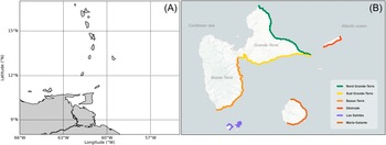
This study focuses on the Lesser Antilles arc (cf., Figure 1A), and the data used covers the period from January 1, 2019, to December 31, 2023. However, some daily data from 2018 have been added as input to our methods to improve automatic analysis. The datasets used take the form of matrices of numerical values, providing geolocalized information on physical and environmental parameters. The data sources used are presented in the following subsection.
(A) Study area: Lesser Antilles arc from 55 to 66°W and 8 to 17°N. (B) Guadeloupe coastlines: Nord Grande-Terre (NGT) in green line, Sud Grande-Terre (SGT) in yellow line, Basse-Terre (BT) in orange line, Désirade in red line, Les Saintes (LS) in purple line, and Marie-Galante (MG) in brown line.

Figure 1. Long description
Panel A is a large-scale map with a grid. The y-axis represents Latitude in degrees North from 9 to 15. The x-axis represents Longitude in degrees West from 66 to 57. It shows the chain of islands in the Lesser Antilles and the northern coast of South America in the Southwest corner.
Panel B is a detailed map of Guadeloupe. The Caribbean Sea is labeled to the West and the Atlantic Ocean to the East. The main island is divided into Basse-Terre on the West and Grande-Terre on the East. Colored lines highlight specific coastal segments as follows.
* Nord Grande-Terre is marked with a green line along the Northeast coast.
* Sud Grande-Terre is marked with a yellow line along the Southeast coast.
* Basse-Terre is marked with an orange line along its entire Western and Southern coast.
* Désirade is an island to the East marked with a red line on its Northern coast.
* Les Saintes are small islands to the South marked in purple.
* Marie-Galante is a circular island to the Southeast marked with a brown line on its Eastern coast.
Before being used in automatic analysis methods, each dataset is subjected to internal normalization (cf., Equation 1) to optimize the operation of the algorithms, as follows:

where
$ D $
 represents a dataset (i.e., all days within the study period),
$ d $
represents a dataset (i.e., all days within the study period),
$ d $
 represents a data matrix for 1 day, and
$ {d}^{\prime } $
represents a data matrix for 1 day, and
$ {d}^{\prime } $
 the latter after normalization. This operation is performed for each day
$ d\in D $
the latter after normalization. This operation is performed for each day
$ d\in D $
 and for each dataset. For processing purposes, the different datasets were interpolated to a common resolution of 0.08° in longitude and 0.04° in latitude using a bilinear method. The 12:00 Coordinated Universal Time (UTC) forecast data (corresponding to 08:00 AM local time in Guadeloupe) was selected to ensure data availability in the context of daily operational forecasting.
2.1. HYCOM surface current dataset
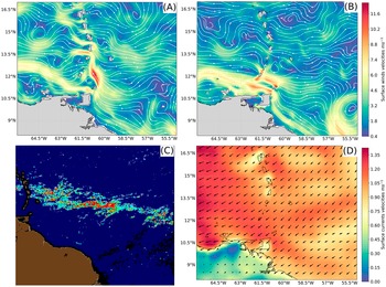
Daily surface current components from the 41-layer Hybrid Coordinate Ocean Model (HYCOM), at 1/12° resolution, global analysis (HYCOM GLBy0.08 version, available at: https://www.hycom.org/data/glby0pt08/expt-93pt0), were examined (Cummings and Smedstad, Reference Cummings and Smedstad2013; Helber et al., Reference Helber, Townsend, Barron, Dastugue and Carnes2013). The HYCOM surface forcing, including 10 m wind velocities, is extracted from Climate Forecast System Version 2 (CFSv2) (cf., Figure 2A). The Navy Coupled Ocean Data Assimilation (NCODA) system is used to assimilate available observational data: satellite altimeter sea surface height, satellite and in situ sea surface temperature, temperature vertical profiles, and salinity vertical profiles. The HYCOM GLBy0.08 grid resolution is 0.08° in longitude and 0.04° in latitude. To perform the present study, the native HYCOM fields were normalized.
Spatial maps of the different predictors for January 1, 2019: (A) HYCOM surface current; (B) Mercator surface current; (C) FA-Density satellite image; and (D) ERA-5 surface winds.
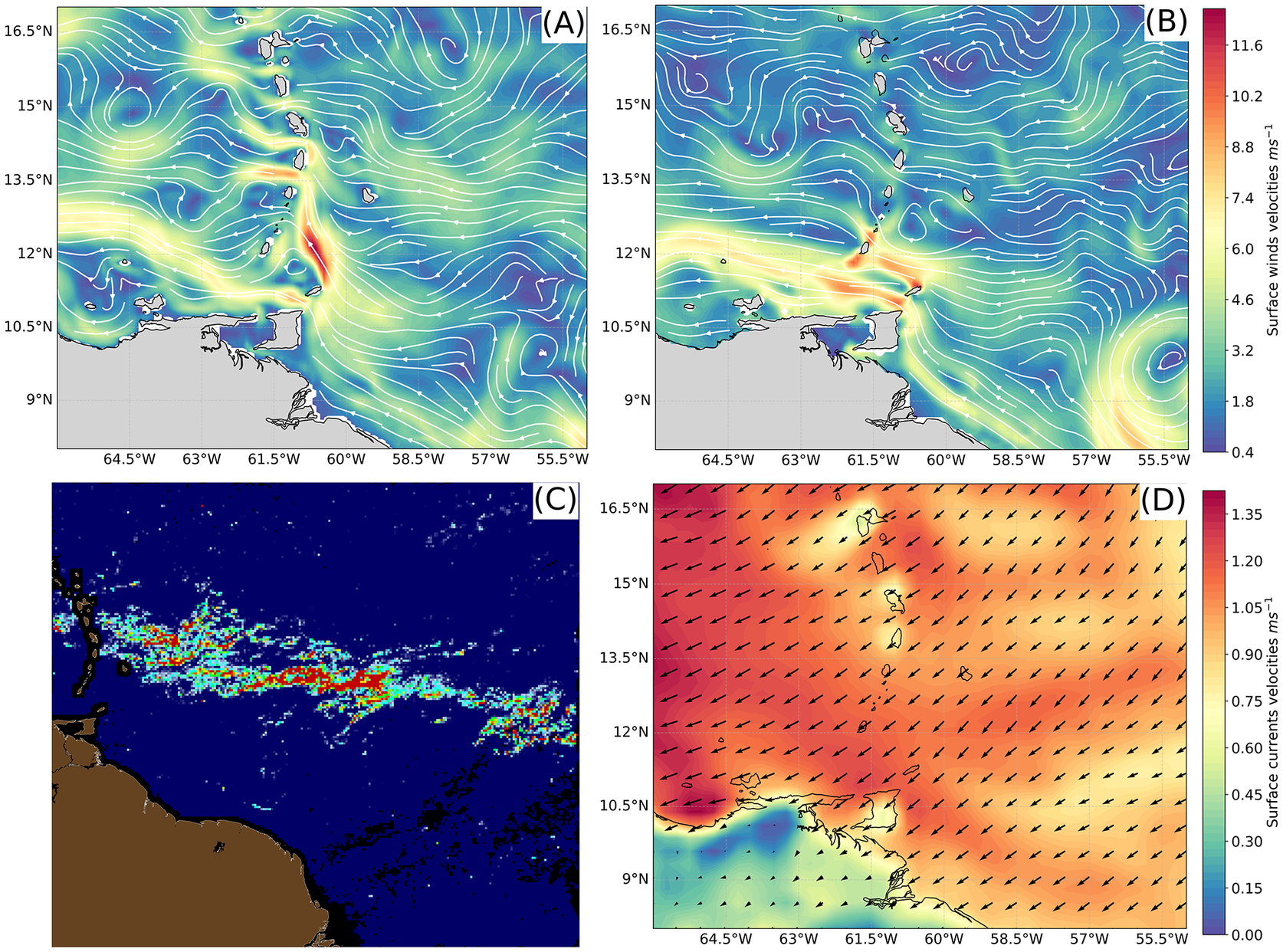
Figure 2. Long description
The figure consists of four panels labeled A through D. All panels share a geographical grid from 9 degrees North to 16.5 degrees North and 65.5 degrees West to 55.5 degrees West.
Panel A and B: Heat maps of surface wind velocities in meters per second (m s super -1). A color scale on the right ranges from 0.4 (dark blue) to 11.6 (dark red). White streamlines show wind flow. In Panel A, high-velocity winds (yellow to red) are concentrated in a channel between the islands around 12 to 13.5 degrees North. Panel B shows a similar pattern but with slightly lower peak intensities and more turbulent streamline swirls in the East.
Panel C: A satellite-style map showing a horizontal band of high-intensity data (red and yellow pixels) stretching from West to East across the center of the frame, likely representing precipitation or cloud cover, against a dark blue background.
Panel D: A heat map of surface current velocities in m s super -1. The color scale ranges from 0.00 (dark blue) to 1.35 (dark red). Black arrows indicate current direction. The highest velocities (orange to red) are found in the open ocean East of the islands, with currents flowing generally Northwest. Lower velocities (blue and green) are visible along the South American coast in the Southwest quadrant.
2.2. Mercator surface current dataset
Daily surface current component data sourced from the Mercator PSY4V3R1 analysis system were utilized. This dataset features a 1/12° resolution with 50-layer 3D analysis and a uniform 0.08° resolution in latitude and longitude (Lellouche et al., Reference Lellouche, Greiner, Le Galloudec, Garric, Regnier, Drevillon, Benkiran, Testut, Bourdalle-Badie, Gasparin, Hernandez, Levier, Drillet, Remy and Le Traon2018). For this study, the data were also normalized and interpolated (cf., Figure 2B).
2.3. ERA-5 dataset: surface winds
Daily surface wind data were also considered, as they have an impact on the transport of Sargassum in the water. Surface wind components with a horizontal resolution of 31 km from the ERA5 reanalysis model (Hersbach et al., Reference Hersbach, Bell, Berrisford, Biavati, Horányi, Muñoz Sabater, Nicolas, Peubey, Radu, Rozum, Schepers, Simmons, Soci, Dee and Thépaut2020) (available here: https://cds.climate.copernicus.eu/cdsapp#!/dataset/reanalysis-era5-pressure-levels?tab=overview) were used (cf., Figure 2D). The data were normalized (cf., Equation 1) and interpolated using a bilinear method, so that the data had the same dimensions as the HYCOM surface current data.
2.4. Satellite-based offshore abundance of Sargassum
We also consider images from several satellites. Floating algae have a particular wavelength, and it is this wavelength that is used to obtain the algae flotation index anomaly (AFAI). However, the heavy cloud cover in the Lesser Antilles leads to temporarily unavailable data on certain days. For this reason, we use the floating algae density index (FA-Density) (cf., Figure 2C), which is obtained from 7 consecutive days of AFAI data. The more algae pass through a zone, the higher the FA-Density. This process gives us images that provide information on the position and density of algae with a resolution of 1°. These data have been normalized and interpolated to have the same dimensions as the HYCOM data.
2.5. Beaching observational data
Observations of Sargassum beachings on the Guadeloupe coast, provided by the Direction de l’Environnement, de l’Aménagement et du Logement (DEAL) de Guadeloupe from 2017 to 2019 and by Météo France from 2020 onwards have been used to create the labels. These labels are the responses that will be given to the neural networks so that they can train themselves.
Two labeling methods were used: for the first method, beaching was considered to have occurred as soon as the probability of beachings in the observation data was high. The result is a matrix with a size corresponding to the number of days between January 1, 2019, and December 31, 2023 (i.e., 1,826 days). The label will be 0 if there are no beachings and 1 if there are. Of the 1,826 days analyzed, 277 days of beachings are observed.
For the second method, only Météo France observations were considered. The bulletins published by Météo France contain the probability of Sargassum algae beachings for Nord Grande-Terre (NG), Sud Grande-Terre (SGT), Basse-Terre (BT), Désirade, Les Saintes (LS), and Marie-Galante (MG) (cf., Figure 1B). Forecasts are valid from the day of issue of the bulletin and for the following 3 days. For each bulletin we had available, the probability of beachings for each zone was assigned to the date on which the bulletin was published and to the three following days. The other dates were initialized to 0 for all zones. The result is a matrix with the following dimensions (1,461, 6), where 1,461 is the number of days in the period from January 1, 2020, to December 31, 2023, and 6 is the number of zones. Over this period, there are 1,027 days where there is a risk of beachings and 434 where there is no risk.
2.6. Dataset creation
Convolutional neural networks (CNN) can process input data tensors or handle input data with variable depth. In the case of images, a CNN processes an input with a depth comprising three color channels (Red, Green, and Blue) (Taye, Reference Taye2023). So, we are going to build our own tensors from the data presented in the previous section. In this case, the input data will have a seven-level depth. These are seven separate parameters: the
$ {U}_0 $
 and
$ {V}_0 $
and
$ {V}_0 $
 components of the surface currents from the HYCOM and Mercator models, the
$ U $
components of the surface currents from the HYCOM and Mercator models, the
$ U $
 and
$ V $
and
$ V $
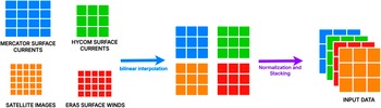
 components of the wind, and finally, satellite measurements of Sargassum density. To build the data tensors, we first resized each dataset so that they all had the same dimensions: those of the HYCOM model. We then normalized each dataset and stacked the parameters for each day one after the other (cf., Figure 3). We thus end up with a tensor of dimensions (1,826,
$ 7\times n $
components of the wind, and finally, satellite measurements of Sargassum density. To build the data tensors, we first resized each dataset so that they all had the same dimensions: those of the HYCOM model. We then normalized each dataset and stacked the parameters for each day one after the other (cf., Figure 3). We thus end up with a tensor of dimensions (1,826,
$ 7\times n $
 , 226,138) Here, each element of the tensor represents 1 day of the study period,
$ n $
, 226,138) Here, each element of the tensor represents 1 day of the study period,
$ n $
 represents the number of input days supplied to the neural network, and each day consists of seven variables. This tensor represents the dataset that will be used in the two approaches presented in the following sections.
Data preprocessing: The satellite images and the components
$ U $
 ,
$ V $
,
$ V $
 ,
$ {U}_0 $
,
$ {U}_0 $
 ,
$ {V}_0 $
,
$ {V}_0 $
 are resized, normalized, and stacked to a tensor (1,826,
$ 7\times n $
are resized, normalized, and stacked to a tensor (1,826,
$ 7\times n $
 , 226,138).
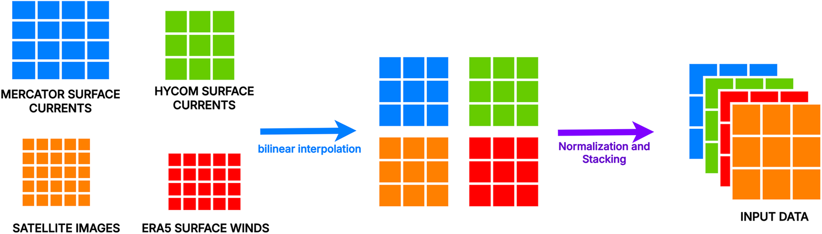
This flowchart shows how the input data matrices are prepared for the neural network.
At first, the four environmental datasets (Mercator Surface Currents, HYCOM Surface Currents, Satellite Images, and ERA5 Surface Winds) have different grid dimensions. A blue arrow labeled “bilinear interpolation” indicates that they are all resized into a single, uniform grid size. Finally, a purple arrow labeled “Normalization and Stacking” shows that these uniform matrices are combined together to create the final multi-channel “INPUT DATA” tensor.
2.7. Classification models
Before building a new network, the possibility of transfer learning was mentioned. This involves using a model that has already been trained for a task similar to the one we want to perform and adapting it to our problem. This method reduces the immense time and resource demands of training most neural network models. Pretrained models exist for solving problems related to Sargassum algae (Wang and Hu, Reference Wang and Hu2021; Laval et al., Reference Laval, Belmouhcine, Courtrai, Descloitres, Salazar-Garibay, Schamberger, Minghelli, Thibaut, Dorville, Mazoyer, Zongo and Chevalier2023); however, none of these models use the data presented in this study, and none are focused on the area presented. For this reason, the models presented below are built from scratch. To build our model for forecasting Sargassum algae arrivals, we began by designing a classification model using convolutional neural networks. Our objective is to assign a class to every entry in the dataset.
In this study, two classes are considered: days with beachings and days without beachings. As mentioned in Section 2.5, out of 1,826 days, there are only 277 days with beachings, and therefore 1,549 days with no beachings. We note a class imbalance, which could affect the ability of our models to assign the right class to each day, due to the low number of examples of days with beachings. To address this issue, the class representing beaching days was oversampled. This was achieved by duplicating samples of beaching events until class parity was reached, resulting in a newly balanced dataset. While other techniques, such as SMOTE or data augmentation, were considered, they were dismissed as they could alter the physical properties and spatial coherence of the data, elements we specifically aimed to preserve. This dataset was then split into a training dataset and a test dataset using a 70:30 ratio, resulting in 2,168 training samples and 930 testing samples. Both the training and testing sets maintain a perfect parity between beaching and nonbeaching events.
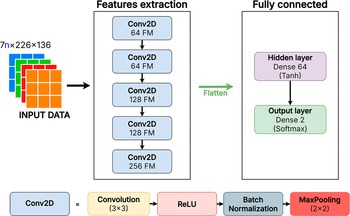
Each CNN consists of five feature extraction blocks followed by a fully connected network, which is in fact a multilayer perceptron. Each feature extraction block consists of a convolutional layer using kernels of size
$ 3\times 3 $
 , followed by a batch normalization (BN) and a max pooling layer of size
$ 2\times 2 $
, followed by a batch normalization (BN) and a max pooling layer of size
$ 2\times 2 $
 . Thus, at the output of the pooling layer, several feature maps (FMs) are extracted. The first two blocks generate 64FM, 128FM is produced at the next two layers, and finally, the last block extracts 256FM. The feature maps produced in the last block are then vectorized to be passed as input to the fully connected part, which handles classification (cf., Figure 4).
CNN-based architecture for classification;
$ n $
 corresponds to the number of days provided as input.
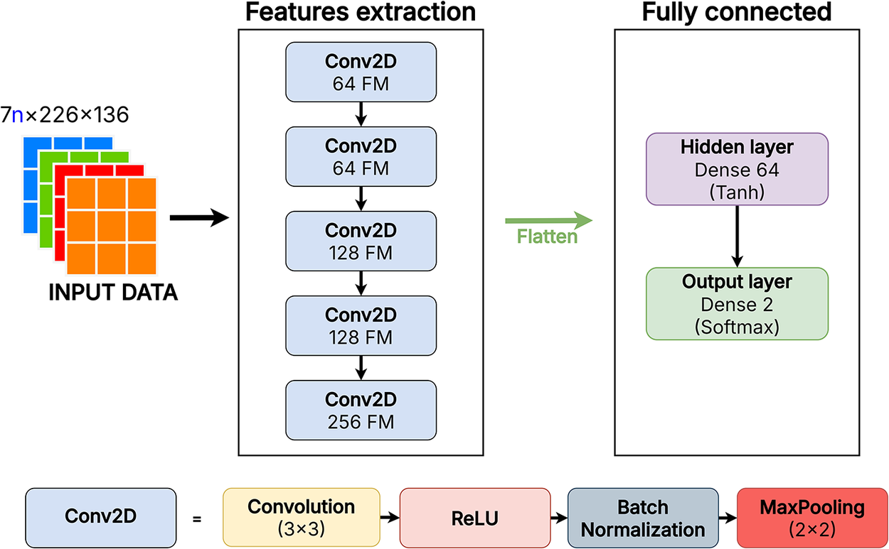
Figure 4. Long description
This flowchart describes the architecture of a Convolutional Neural Network (CNN) used for Sargassum classification.The process starts on the left with the multi-channel “n” input data tensor. This input passes sequentially through a vertical stack of five convolutional blocks labeled Conv2D. The first two blocks generate 64 Feature Maps (FM), the next two generate 128 FM, and the final block generates 256 FM. The legend at the bottom indicates that each Conv2D block combines a 3 × 3 Convolution, a ReLU activation, a Batch Normalization, and a 2 × 2 MaxPooling. An arrow labeled “Flatten” shows the transition from the convolutional features to the fully connected layers. This leads to a “Hidden layer” (Dense 64 with Tanh activation) and finally to an “Output layer” (Dense 2 with Softmax activation) which delivers the final classification results.
The class assignment part has a single hidden layer, containing 64 neurons. The output layer is made up of two neurons, corresponding respectively to the class of days without beachings and that of days with beachings. Finally, the ReLU activation function is used for the convolutional layers. For the classification part, the hyperbolic tangent function is applied to the hidden layer, while the softmax function is used for the output layer. The results obtained are detailed in Section 3.1.
2.8. Regression models
Still with the aim of predicting the arrival of Sargassum seaweed, a second approach was tested. This approach consists of a model with six neurons on its output layer, each of which corresponds to a Guadeloupe coastline (cf., Figure 1B). The output value indicates the probability of Sargassum arriving on the coast concerned. These models will be referred to as “
$ ZonalReg $
 ” models. For these models, oversampling was not used because the task shifted from a classification problem to a regression problem, where the class imbalance issue is negligible. Furthermore, as previously mentioned, the Météo France bulletins provided beaching probabilities for each zone over a 4-day period. The dataset for these models was also split using a 70:30 ratio, resulting in a training set of 1,022 examples and a test set of 439 examples.
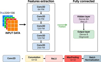
The architecture of the feature extraction part is almost identical to that presented for the classification model. The only difference is that the Batch Normalization and Max Pooling layers in the Conv2D block have been inverted. The number of neurons on the output layer of these models changes since the aim is not to assign a class to each entry, but to provide a probability of beachings per zone. For the same reason, the activation function used on the output layer is no longer the softmax function but the sigmoid function. Finally, the activation function used on the hidden layer of the fully connected part is the ReLU function (cf., Figure 5). The results of experiments with these two models will be detailed in Section 3.2.
$ ZonalReg $
 model architecture, where n corresponds to the number of days provided as input.
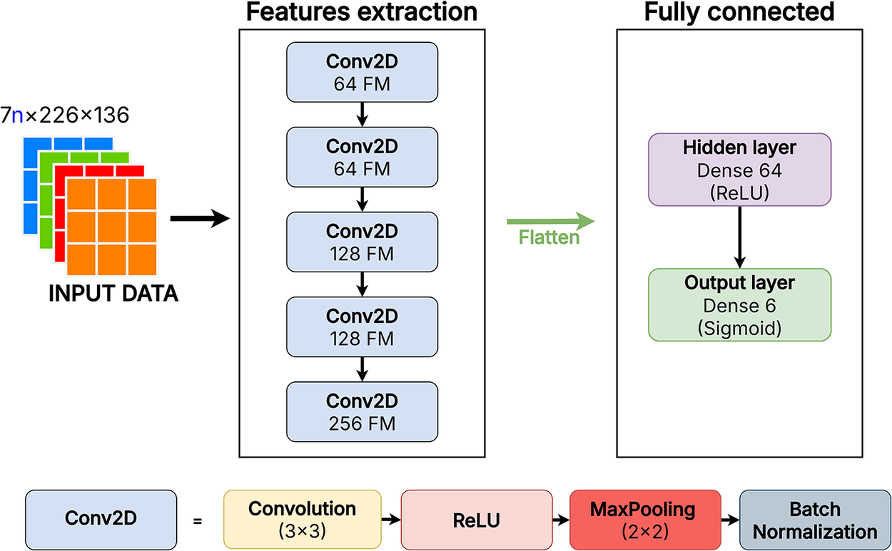
Figure 5. Long description
This flowchart describes the architecture of a Convolutional Neural Network (CNN) used for Sargassum zonal regression.The process starts on the left with the multi-channel “n” input data tensor. This in the bottom indicates that each Conv2D block combines a 3 × 3 Convolution, a ReLU activation, a 2 × 2 MaxPooling, and a Batch Normalization. An arrow labeled “Flatten” shows the transition from the convolutional features to the fully connected layers. This leads to a “Hidden layer” (Dense 64 with ReLU activation) and finally to an “Output layer” (Dense 6 with Sigmoid activation) which delivers the final regression outputs.
3. Results and discussions
To achieve optimal performance, extensive experiments were conducted by varying key hyperparameters, including the learning rate, batch size, the number of days provided as input to the network, and the forecast lead time. The models were implemented in Python using the TensorFlow library and the Keras API. Furthermore, the training loops were executed on the C3I high-performance computing cluster of the University of the Antilles, enabling the development of models capable of predicting beaching events up to 14 days in advance. Among the configurations tested, the most effective models were those utilizing a single day of input data, represented as tensors of seven parameters.
To evaluate model performance, distinct metrics were employed for both classification and regression tasks. Classification results were assessed based on accuracy, sensitivity (recall), and specificity (cf., Supplementary Appendix A.1, A.2, and A.3). For the regression analysis, the mean absolute error (MAE) and the root mean square error (RMSE) (cf., Supplementary Appendix A.4 and A.5) were utilized to quantify predictive precision. Furthermore, to enable a direct comparison between the two approaches, classification metrics were also calculated for the regression models. This was achieved by applying a threshold of 0.5 to the continuous outputs, thereby transforming the regression results into binary classifications. Beyond these performance metrics, identifying the specific contribution of each input variable to the model’s predictions remains a key objective for future analysis. To determine which predictor has the greatest impact on the forecasts, an interpretability study using Integrated Gradients (Sundararajan et al., Reference Sundararajan, Taly and Yan2017; Singh et al., Reference Singh, Konovalova and Kar2023) could be conducted. This method would provide a more transparent understanding of the underlying physical mechanisms captured by the network, moving beyond simple scores to explain how specific parameters influence beaching events.
Due to the method used for class rebalancing, which involves duplicating days with beachings, it is possible that model performance may be overestimated. For the sake of clarity, only a selection of the most pertinent results is presented in this report.
3.1. Classification models
Table 1 Supplementary Appendix B.1) details the performance of the 15 classification models from
$ D+0 $
 to
$ D+14 $
to
$ D+14 $
 , with best and worst scores highlighted in green and red, respectively. Performance is consistently high, with average accuracy, specificity, and sensitivity reaching 94.75%, 97.42%, and 98.79%, respectively. The
$ D+14 $
, with best and worst scores highlighted in green and red, respectively. Performance is consistently high, with average accuracy, specificity, and sensitivity reaching 94.75%, 97.42%, and 98.79%, respectively. The
$ D+14 $
 model achieves peak accuracy and specificity, while the highest sensitivity is shared by the
$ D+0 $
model achieves peak accuracy and specificity, while the highest sensitivity is shared by the
$ D+0 $
 and
$ D+2 $
and
$ D+2 $
 models. Even the minimum scores remain robust, exceeding 93% across all metrics. The high specificity reflects the model’s effective handling of class imbalance, accurately identifying the predominant “no-beaching” days. Simultaneously, the strong sensitivity scores demonstrate the model’s capability to correctly detect actual beaching events. Overall, these results indicate that the networks successfully capture the underlying patterns for both classes across the entire 14-day forecast horizon
3.2. ZonalReg models
Tables 2 and 3 (cf., Supplementary Appendix B.2 and B.3) show the evaluation of metrics for the 15 zonal regression models. The regression analysis reveals that both MAE and RMSE values exhibit minimal variation across the different models, maintaining consistently low levels with an average error of 0.13 and 0.18, respectively. This remarkable stability in error margins indicates that the network’s predictive precision remains robust throughout the entire forecasting range. Consequently, the models can deliver stable and accurate predictions up to a 14-day lead time without significant degradation in performance.
In Table 3 (cf., Supplementary Appendix B.3), the optimal scores for each metric are highlighted in green, while the lowest performances are indicated in red. The scores for accuracy, sensitivity, and specificity derived from these regression models demonstrate strong results. Specifically, we observed a maximum (minimum) accuracy of 92.74% (88.16%), sensitivity of 89.89% (76.97%), and specificity of 98.96% (95.80%). Although these results are high, they remain slightly below those of the dedicated classification models. This difference can be explained by the application of a fixed threshold to the continuous outputs; unlike classification models, this method leaves less margin for error.
Despite slightly lower classification scores, the regression approach provides superior geographical precision. While we initially considered a multimodel classification approach consisting of six classifiers, one for each zone, to determine whether or not a zone would be affected, we chose to develop these regression models to provide the beaching probability for each zone. This allowed us to quantify the level to which each area is affected rather than simply stating if an impact occurs. Consequently, the regression models deliver specific predictions for each coastal zone, whereas classification models only offer a single global output for the entire coastline.
4. Conclusion and perspectives
The objective of this study was to build a convolutional neural network model capable of predicting the arrival of Sargassum algae on the coasts of Guadeloupe. This model was intended to use data on winds, surface currents, satellite images, as well as observations of beachings and arrivals of these algae on the shores. To achieve this goal, several classification and regression models were proposed. Both approaches demonstrated superior performance compared to the traditional decision tree proposed in a previous study, which achieved scores of 70.10% for accuracy, 73.10% for sensitivity, and 69.20% for specificity. In comparison, the proposed CNN models reached significantly higher results, with accuracy up to 95.70%, sensitivity of 99.64%, and specificity of 98.96%; the regression models also achieved an average MAE of 0.13 and an average RMSE of 0.18, confirming that deep learning architectures are better suited for capturing these complex dynamics over a 14-day lead time.
A significant advantage of this study lies in the geographical precision of regression models. Although classification models achieved higher metrics, the regression approach is more relevant for precise monitoring. Despite a slight performance gap, which can be explained using a fixed threshold, these models deliver specific predictions for each coastal zone rather than a single global output.
This study currently demonstrates that there is a significant predictability within the data that can be effectively learned by the models. However, as these models were trained on reanalysis data, it would be valuable to investigate whether similar performance levels are maintained when using real-time operational data. Future work could focus on improving regression scores to bridge the performance gap, notably by identifying an optimal threshold through ROC curve analysis for a more balanced comparison. Furthermore, analyzing with Integrated Gradients could help determine which predictors have the greatest impact on the forecasts. Furthermore, the robust performance observed even at a 14-day lead time encourages us to extend the forecasting horizon in subsequent studies to provide earlier warnings for coastal management.
Supplementary material
The supplementary material for this article can be found at http://doi.org/10.1017/eds.2026.10053.
Acknowledgements
The authors would like to thank the reviewers for their valuable comments and suggestions, as well as the Centre Commun de Calcul Intensif (C3I) at Université des Antilles for providing the computational resources and high-performance computing facilities used in this work.
Author contribution
E.B.: Conceptualization; R.B. and E.B.: Methodology; R.B., E.B.: Data curation; R.B.: Data visualization; R.B., E.B.: Writing—original draft; V.P., D.B., R.C., A.D.: Reviewing. All authors approved the final submitted draft.
Competing interest
The authors declare none.
Data availability statement
The study utilizes publicly available datasets: ERA5 reanalysis from the Copernicus Climate Data Store, oceanic products from the E.U. Copernicus Marine Service (Mercator Ocean), and HYCOM model outputs from the HYCOM Consortium data server. All original data can be accessed via their respective official portals. The source code developed for this study and the data are publicly available at https://doi.org/10.5281/zenodo.20618023. By utilizing these provided materials, all the results presented in this study can be reproduced.
Funding statement
This research received no specific grant from any funding agency in the public, commercial, or not-for-profit sectors.
Provenance statement
This article is part of the Climate Informatics 2026 proceedings and was accepted in Environmental Data Science based on the Climate Informatics peer review process.





 Open access

