


1. Introduction
The last years have witnessed a proliferation of machine learning tools and methods in the design community, in various academic and industrial fields. While most of these methods, when related to design problems, are implemented towards classification and prediction tasks, the more recent developments of deep generative models such as variational autoencoders (VAEs) and generative adversarial networks (GAN) have opened a different and appealing window of possibilities within a core area of design disciplines such as generative design.
In design disciplines, the need for alternatives to a known design is a classic situation. It manifests itself as a search for variations that can resemble certain characteristics of the original known design, whilst being original in their own right. Deep generative models can help tackle such challenges, by producing output samples that resemble features of the input sample. Being probabilistic models, they allow for interpretable representations and measurable output predictions, in addition to the adaptability and learning scalability of deep neural networks. This research area – which includes VAEs, GAN, and more – is one of the most exciting and rapidly evolving fields of statistical machine learning (Cunningham Reference Cunningham2019).
The present work focusses on the use of VAEs (Kingma & Welling Reference Kingma and Welling2014) models, which are a special kind of autoencoder that enforce a continuous distribution in their latent space. By sampling from a continuous latent space, these models generate new objects that inherit features from the samples present in the training set, but are at the same time essentially unique. This study follows up on previous work where the notion of a ‘connectivity vector’ was developed, which represented the geometrical 3D object in a network fashion. This encoding resulted in a data set of high-dimensional vectors.
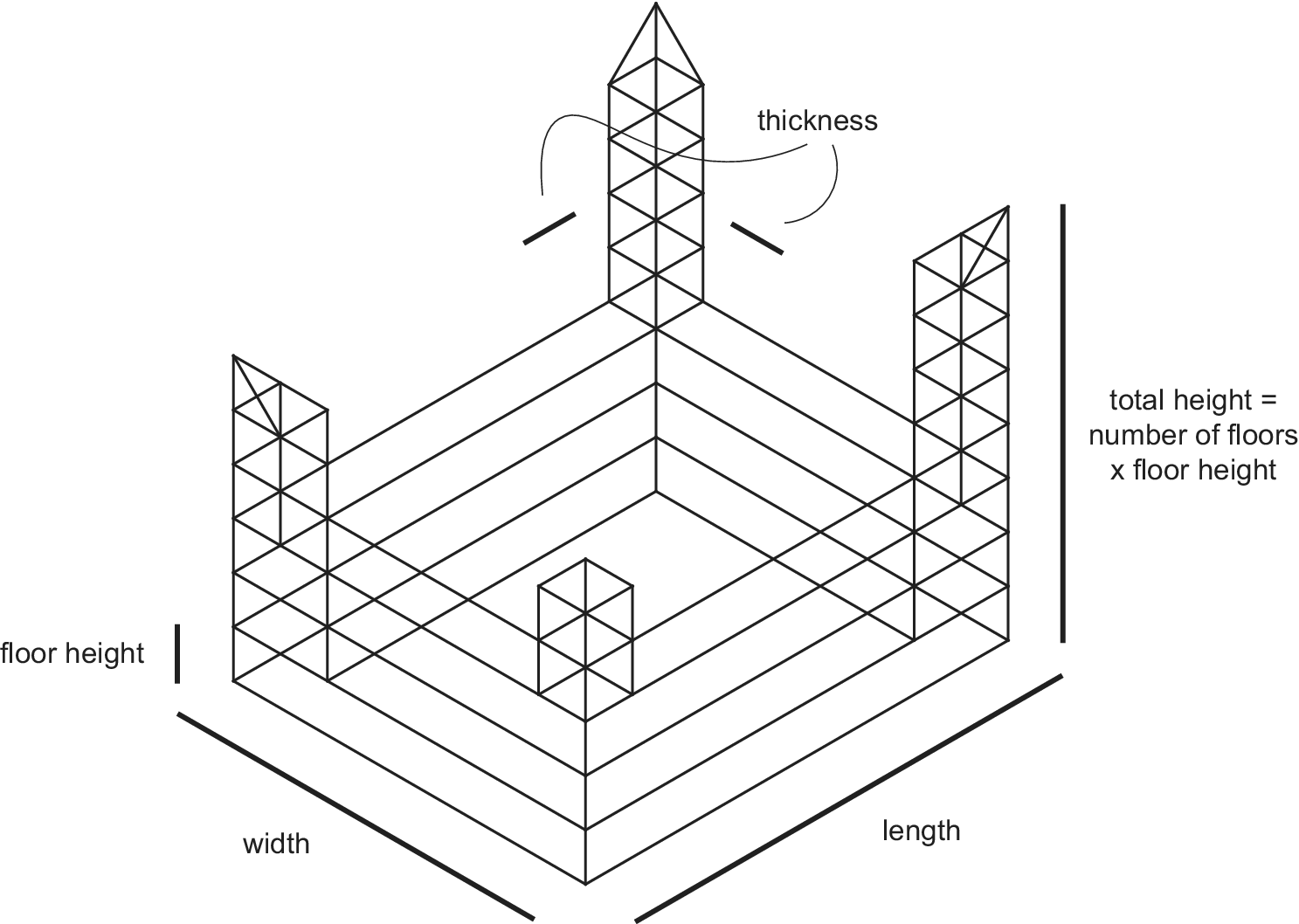
By leveraging the way data are encoded, geometrical 3D objects can be expressed as tensor-shaped input data sets for training. Thus, the challenge becomes the balance of the high number of parameters of the model, especially when relative to the amount of samples in the training set. The work presented in this paper handles input composed of high-dimensional vectors containing the data of geometrical objects. These objects will be called ‘building types’, since they are simplified representations of the geometry of more sophisticated architectural building objects. These are inspired by the structural wireframes of these building geometries. By taking a simplified set of centre lines of the interconnected structural elements that compose an architectural object in 3D space, a wireframe is created. Thus, this wireframe is representative of the core geometry of the building type. Described by connectivity vectors, this geometrical object is used as input data for a VAE model, opening up a methodology within machine learning applied to 3D objects that is applicable to the field of architectural design.
VAE models are shown to be able to generate many types of complex data. Although initially trained on sets of 2D images, proliferated use of these models in wider disciplines has driven the need for working with vector data and 3D geometry (Gregor et al. Reference Simonyan and Zisserman2015; Ha & Eck Reference Ha and Eck2018). Various works within the design community that map the potential of this approach have already been conducted (Cudzik & Radziszewski Reference Cudzik and Radziszewski2018). Powerful techniques inherent to deep generative models like sampling (White Reference White2016) and feature vector arithmetic (Radford, Metz & Chintala Reference Radford, Metz and Chintala2016) show great promise in the context of design.
Deep generative models typically require large data sets for training purposes. Working with representations of structural building types allows for the implementation of parametric tools for data augmentation. This is due to the fact that building types allow for individual samples to have various discrete yet observable characteristics that enable them to be identified as part of a given family or type. In the experimentation section, an account of the experiments conducted is presented. In these tests, a VAE model trains on an augmented data set and learns to extract features that are characteristic of the input building types. In the last stage of the process, the generative capability of the network is used by sampling new points from the continuous latent distribution that the model has learnt. The decoder then outputs their corresponding connectivity maps that result in newly generated building types.
The work presented in this paper is intended to improve the results obtained throughout the experiments conducted during the development of this method (de Miguel et al. Reference de Miguel-Rodriguez, Villafañe, Piškorec and Sancho-Caparrini2019), leading to overfitting of the learning process of model, such as the following: (i) due to high dimensionality inherent to the technique used for encoding 3D-objects, a large number of samples were required to train the model; (ii) limited geometrical variation of the types at training and validation sets and, (iii) models with densely connected layers resulted in a very high number of parameters (150 M+ trainable parameters). This paper explores the following solutions to the aforementioned problems: firstly, the development of a parametric data augmentation scheme that enhances geometrical variation. Secondly, the implementation of convolutional layers within the architecture of the model, helping to reduce the number of parameters of the model while maintaining a strong capacity to learn complex patterns. Lastly, a constrained variant of the parametric augmentation method that allows for the limitation of the feature spread of the geometries that compose the data set.
The work presented in this paper seeks to serve as a starting point for exploring future avenues of generative design, especially when in search of alternatives to a known building configuration. The main contribution of this paper is to provide new insights into how parametric augmentation techniques might improve VAE learning in the context of 3D building wireframes. Despite the fact that the current output is still very much a work in progress, the resulting 3D wireframes can be conceived as the first step towards the interpolation of geometries from a set of known input types. Thus, this methodology can serve for experimentation and be further explored by architectural design disciplines. This is only a snippet of the possibilities that this methodology can unlock.
This paper begins with an introduction to the methodology and the motivation igniting this work, and is followed by a brief review of the state of the arts techniques and related works as implemented in similar contemporary research projects. The methodology section is arranged in three parts: data representation, VAE and network architecture. In the first part, a detailed description of the methods used for data representation is presented: A parametric approach to data augmentation, and the improvements brought through its implementation. Then, a description of the encoding method based on the concept of a 3D-canvas with voxelized wireframes is presented: In this 3D-canvas, the input geometry of the building types is represented through their connectivity map and augmented to increase the size of the training set. This is followed by a description of the revised neural network architecture used: VAE model, now with convolutional layers. The model learns a continuous latent distribution of the input data from which it is possible to sample and generate new geometry instances, essentially hybrids of the initial input geometries. Finally, results of these computational experiments are presented, as well as conclusions and outlook for future research in this field.
2. Literature review
Creating new instances based on information of known references is a classical necessity within design disciplines. From an initial known design, one could desire to preserve some of its features by ‘importing’ these into a family of new designs, conceived as variations of the original one. Generating this family of new designs is a task that can be addressed with either manual or computational methods. However, one could argue that both of these types of methods could be ‘algorithmically’ addressed: by identifying the design features that one may wish to preserve (so that they are found within the instances of the new family of designs), a set of rules can be specified so that the selected features are applied with different gradients, making each instance unique yet identifiable as part of a design family of shapes (Gips & Stiny Reference Gips and Stiny1972).
However utilitarian, tools of this nature may support the creative production within design disciplines, by offering a dynamic way of obtaining variations of the known reference for further evaluation. This latter evaluation shall be performed with tools of a rather serviceable nature. In this regard, machine learning techniques for 3D shapes are implemented in various different tasks of geometry manipulation for evaluation purposes. These tasks can be classified in the following categories: Single object classification (Maturana & Scherer Reference Maturana and Scherer2015; Wu et al. Reference Wu, Zhang, Xue, Freeman and Tenenbaum2016a), 3D pose estimation (Wu et al. Reference Wu, Xue, Lim, Tian, Tenenbaum, Torralba and Freeman2016b), multiple objects detection (Song & Xiao Reference Song and Xiao2016), scene-object semantic segmentation (Kalogerakis et al. Reference Kalogerakis, Averkiou, Maji and Chaudhuri2017), 3D geometry synthesis-reconstruction (Pavlakos et al. Reference Pavlakos, Choutas, Ghorbani, Bolkart, Osman, Tzionas and Black2019) and many other categories that are serviceable to the technical aspects of working with 3D geometry.
When related to design disciplines, some machine learning research projects around production of 3D objects delve into techniques where deep generative models actually operate with 2D data sets. Thus, after training, a geometric entity in 3D space can be assessed as a result constructed from the information acquired from the 2D output of the model (Kelly et al. Reference Kelly, Guerrero, Steed, Wonka and Mitra2018; Wang et al. Reference Wang, Ceylan, Popovic and Mitra2018; Hoyer, Sohl-Dickstein & Greydanus Reference Hoyer, Sohl-Dickstein and Greydanus2019). An implementation of this technique in the field of architectural design, for generating new instances of 2D graphs representing architectural layouts of living units, finds inspiration in ‘composing high performing parts of separate design entries into a new whole’ (As, Pal & Basu Reference As, Pal and Basu2018).
The work reviewed in this section is impressive in terms of innovation and wide implementation of novel deep learning algorithms developed in the recent years. In the spirit of establishing a comparison of research efforts, three papers have been selected, since the work they present offers clearly similar efforts as well as starkly different approaches for overcoming challenges around the task of generating 3D designs. The papers for comparison are VoxNet: A 3D Convolutional Neural Network for Real-Time Object Recognition (Maturana & Scherer Reference Maturana and Scherer2015), MeshCNN (Hanocka et al. Reference Hanocka, Hertz, Fish, Giryes, Feishman and Cohen-Or2019) and Generative Deep Learning in Architectural Design (Newton Reference Newton2019).
In terms of similar research efforts around shape representation, MeshCNN proposes a workflow where 3D objects are represented as tetrahedron meshes, and the connectivity of the edges of each mesh informs the architecture of the model, by accounting for the size of the convolutional layer. In a similar spirit, the work presented in this paper relies heavily on vectors denoting the connections between points in 3D space. These points are evenly distributed across space within an envelope where the building wireframes are constructed. This space will be called ‘3D-canvas’.
However, in the work of MeshCNN, meshes are nonuniform representations of the shapes. Since these are essentially numbered point clouds, the objects result in irregular structures. Different to this approach, the methodology presented in this paper operates in a 3D-canvas of consistent size and spacing, thus obtaining uniform representations of shapes across all building types present in the data sets.
In the work of Newton and Maturana, the 3D objects present in the data set are denoted in a consistently sized 3D envelope (‘occupancy grid’, in the work of Maturana), using voxels within this 3D space. This differs from the work presented in this paper, where a connectivity vector carries the information of the lines present at each point of the 3D-canvas. This format, bespoke to the connectivity within the 3D-canvas, finds inspiration in the more classical way of encoding images for neural networks – for example, stacking pixel values of an image along a vector. This format lends itself to carrying more information of the wireframe if required, for each point in this 3D space, thus becoming a flexible way of portraying the information of each sample of the set.
In terms of similar research efforts around model architecture, the work of Hanocka and Maturana utilises convolutional neural networks not for generative purposes but for classification of 3D objects (meshes in the work of Hanocka, voxelised geometries in the work of Maturana), whereas the work of Newton revolves around the implementation of various types of GAN for creation of 2D and 3D designs, assigning one best model architecture to a specific task with a specific shape of data set. The work presented in this paper utilizes VAE, although also a type of generative networks, this is different from GAN due to the aspect of reconstructing data points from the latent scape rather than generating samples by competition within the network.
In terms of similar research efforts around data augmentation, the work presented in MeshCNN makes use of well-defined data sets, with no need of augmenting the number of samples to use for training. However, the works of Maturana and Newton make use of augmentation when dealing with 3D objects, using rotation as the preferred augmentation strategy. These three approaches are different from the one presented in this paper, in that it incorporates a strategy for parametric augmentation, although a similar approach can be found in the work of Newton (Reference Newton2018). It is important to note that implementing this strategy would not be possible in a nonuniform representation shape technique.
Summarizing all the above-mentioned aspects, the work presented in this paper articulates, firstly, a strategy for shape representation based on indexing lines through connectivity vectors. Secondly, a strategy for data set augmentation based on parameters liaizing with variations internal to the type. And, finally, the implementation of VAE, a generative method for the interpolation of new instances stemming from shared attributes of two and potentially more different types. The innovation of this work revolves around the articulation of these three aspects.
3. Methodology
3.1. Data representation: connectivity map
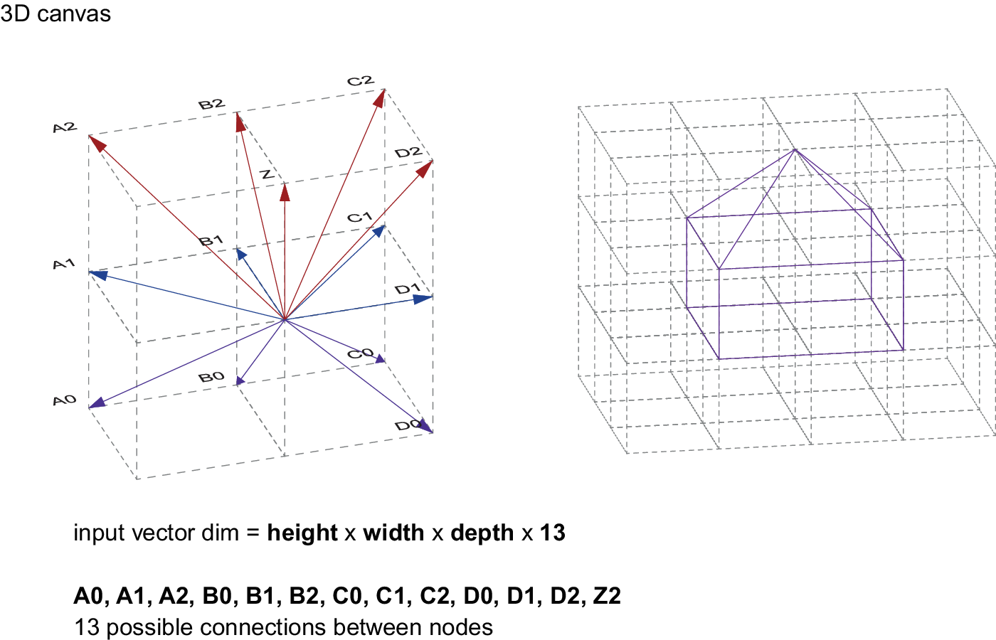
In order to train a VAE, it is crucial to prepare the 3D geometry in a way that can be parsed through the network. This means choosing the most compact way to represent the geometry, avoiding redundancies whilst retaining full information. The scheme presented here is based on a 3D-canvas, which consists of a rectangular 3D volume discretised in cube-shaped cells within which the input geometry is contained. Each cell of the 3D-canvas contains labelled connectivity vectors that can be activated or deactivated depending on the input geometry. These connectivity vectors represent wireframe segments in different orientations that are used to approximate the input geometry in 3D space. To keep the data representation compact and without overlaps, parallel connectivity vectors are discarded and only 13 vectors for each cell are considered, as shown in Figure 1 and Figure 2. To illustrate the scheme, simple geometry and connectivity vectors are depicted in Figure 3 and Figure 4, showing the same principle working in 2D space.
Diagram of the connectivity vector scheme for a 2D geometry.
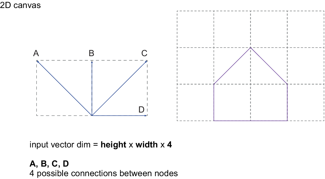
Diagram of the connectivity vector scheme for a 3D geometry.
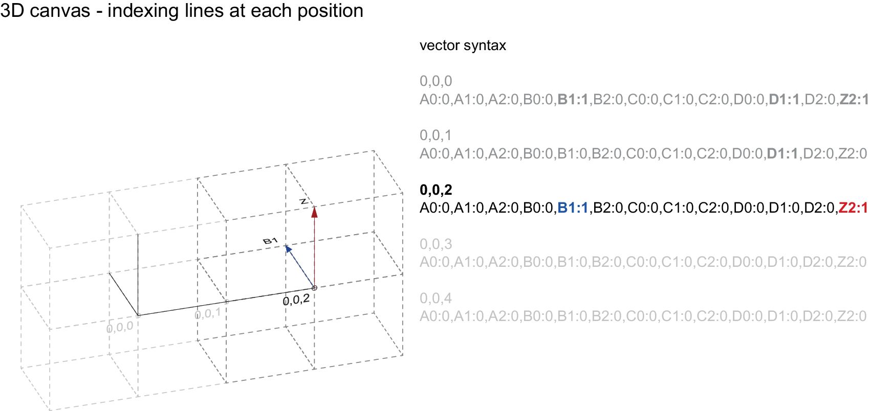
Sequential construction of a 3D building type with the proposed connectivity vector scheme (vector detail).
Sequential construction of a 3D building type with the proposed connectivity vector scheme (geometry detail).
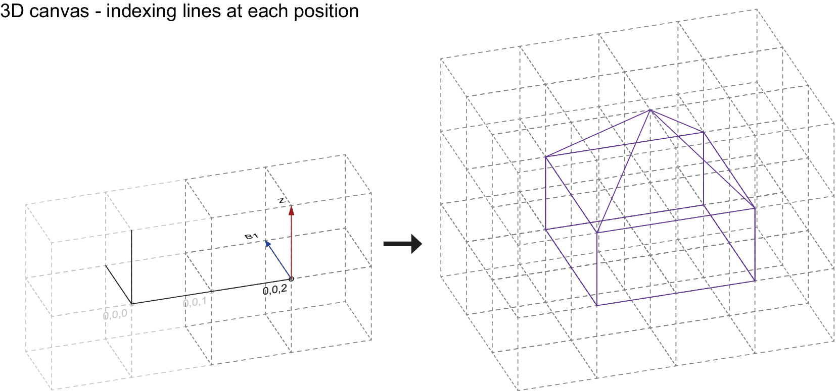
At the beginning of the routine, a 3D-canvas is generated ‘around’ the input geometry, so that the full extent of the input can be encoded within it. Wireframe line segments of the input geometry are then snapped to the grid defined by the cube-shaped cells of the 3D-canvas and corresponding connectivity vectors are mapped according to each one of the orientations of the snapped line segment. This process is iterated throughout each cell of the 3D-canvas (which acts as the container of the input geometry) until the full extent of the input geometry is described in this way. This information is then stored in a set of vectors labelled by their corresponding grid coordinate (3D-canvas) and containing the 13 connectivity values. Each value is marked with a letter and a number indicating its orientation in the cells. In previous work, instead of using a binary value for the presence of a connectivity vector (0 or 1), a continuous value representing a percentage with a domain [0, 1] was used to enhance data augmentation. Although not implemented in the current model, this continuous value could be used in the future to encode the thickness of the structural wireframe element, where smaller values would correspond to thinner elements and larger values to thicker elements. This principle could be used to encode other structural or material properties as well.
Parsing the input geometry into a connectivity map was implemented in Rhino5 using a custom written Python script. The connectivity map itself is stored as a plain text file and read directly by the Python script used to train the VAE. In order to be used as an input, each value from all the connectivity vectors of the 3D-canvas is mapped onto a single input neuron. In the training examples generated, a 3D-canvas with dimensions 21 × 21 × 21 is set up. The 3D-canvas is then composed of 21 cells along the X-axis, 21 cells along the Y-axis and 21 cells along the Z-axis. This resolution is sufficient to distinguish structural types like arches, wall and surface elements, volumes with cavities, openings, etc., allow for the design and implementation of instances of neural networks which are trained for recognition and handling of data pertaining to the field of architectural geometry. With each cell having 13 connectivity vector values assigned to them, the number of input neurons for the VAE is therefore calculated as 21 × 21 × 21 × 13 = 120,393. As the number of training parameters in a neural network grows with the number of input neurons, this size of the 3D-canvas is close to the limit of what can be reasonably dealt with in terms of available computational power.
3.2. Data set generation: parametric data augmentation
Training neural networks of any kind requires large amounts of input data. Additionally, these data should ideally be as continuous as possible in terms of raw input values. For images of 3D objects, this continuity implies gradual changes in translation, rotation, scale, colour and brightness values of the input data. This continuous variation on the level of pixels arises naturally when there are many data samples available. If the number of available training samples is insufficient for conducting a good-quality training, data augmentation can be used as a technique used for increasing the number of training samples by artificially adding variation to the input data (Goodfellow, Bengio & Courville Reference Goodfellow, Bengio and Courville2016). Different augmentation approaches are designed to capture data invariances – changes to the data set, which leave the underlying high-level features unchanged. If implemented correctly, they increase the robustness of the model training by teaching the model to distinguish meaningful from superficial variation in the data set. Standard augmentations for image data are categorised as being either geometric or photometric (Shorten & Khoshgoftaar Reference Shorten and Khoshgoftaar2019). With the exception of noise injection implemented on a geometric level as random probability that any of the connectivity vectors flip its state, only geometric augmentations could be used with 3D wireframe data sets.
Prior to the experiments conducted for this paper, the number of training samples was only two, corresponding to two input models between which the variational autoencoding was to be performed. In previous research (de Miguel et al. Reference de Miguel-Rodriguez, Villafañe, Piškorec and Sancho-Caparrini2019), to augment the training data, simple random translation of the input models was used inside the 3D-canvas to increase the number of training samples to 3000. Initial experiments using rotation as an augmentation strategy were not successful, as rotations in a rectangular grid could not be implemented as gradual transformations but only as 90° steps. These discretely rotated samples would be considered as separate sample categories by the neural network, thus defeating the purpose of the strategy. Similar limitations for scaling the input models were found. Based on these findings, initial experiments used only discrete randomised translation to augment the training data.
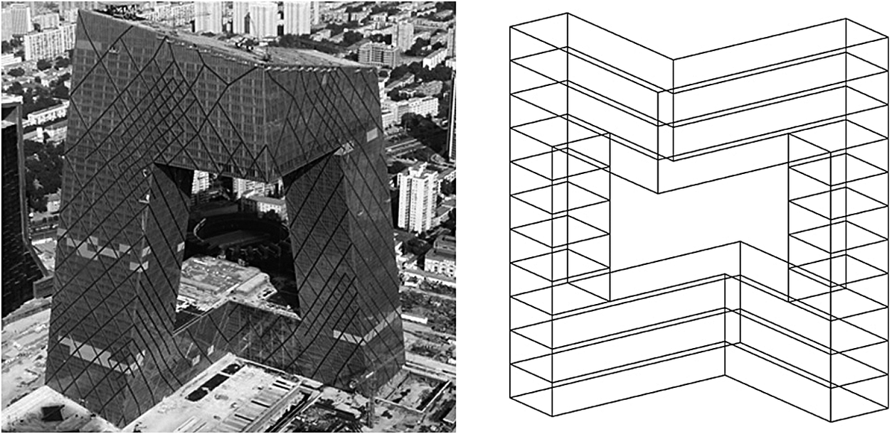
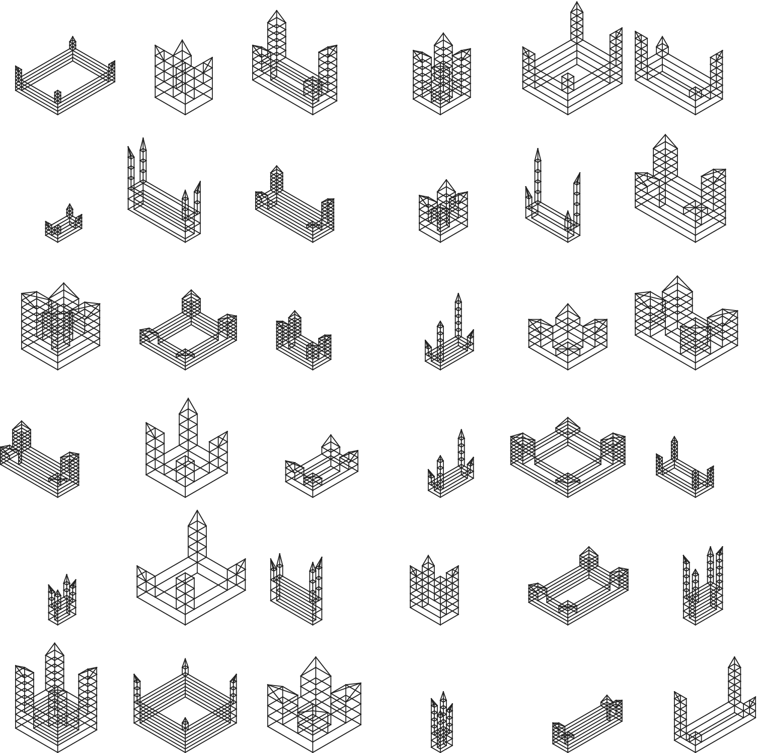
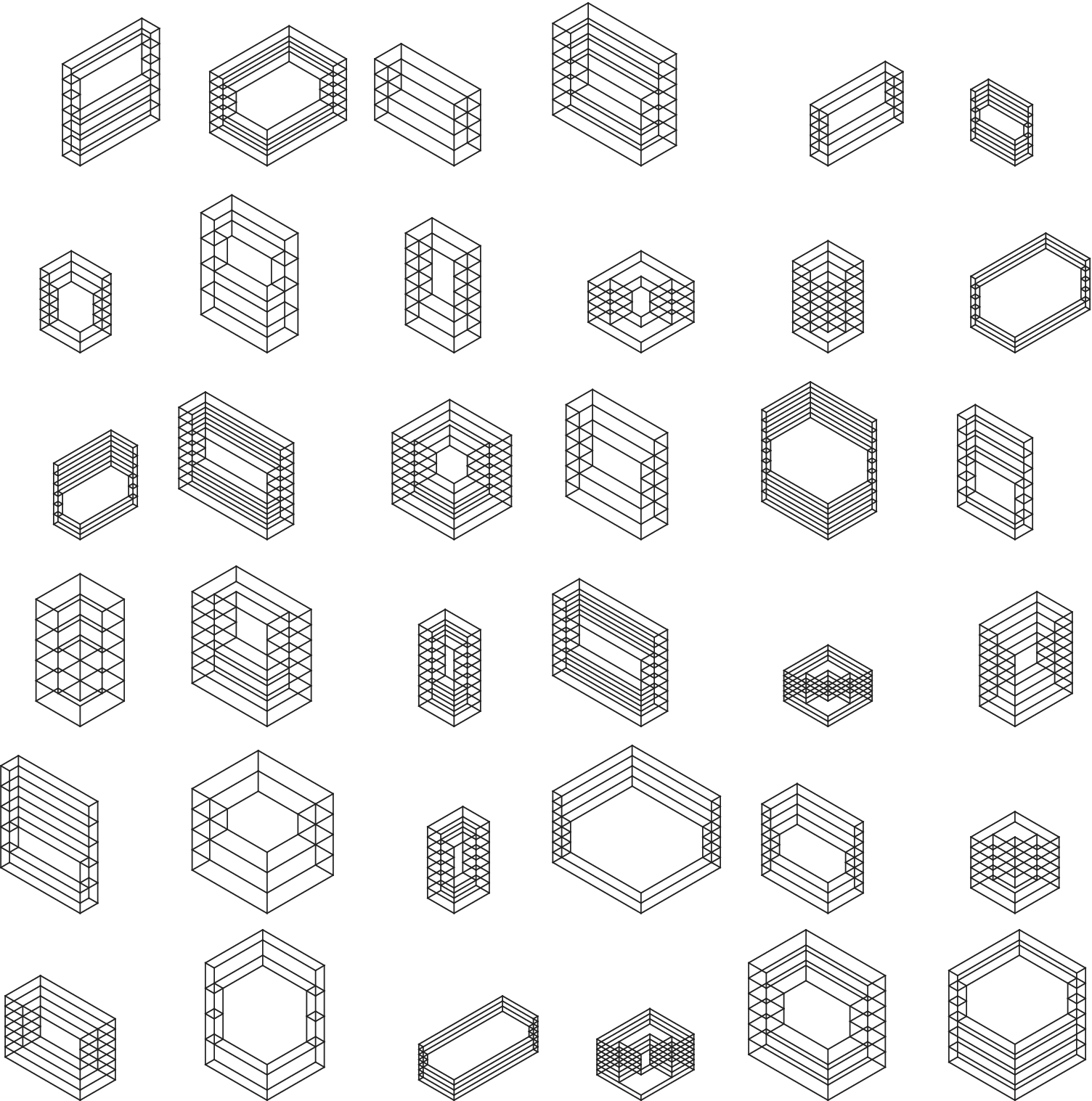
An augmentation technique that is adopted in this paper is parametric augmentation. Instead of manually modelling training samples as 3D wireframes, a stochastic parametric generator is implemented that produces samples satisfying certain constraints. For this paper, the stochastic generator is implemented in the Rhino Python environment for two models: (i) Hejduk-inspired structure (castle) and (ii) CCTV building (China Central Television) (Figure 5). Both model implementations include parameters like total length and width of the model, height of the individual floor, number of floors of different model segments as well as thickness of certain model features (i.e., width of the towers) (Figure 6 and Figure 7). Domains of each of these parameters are fixed by determining minimum and maximum allowable values. Generation proceeds by randomly sampling these domains from a uniform distribution. As it is sampled only from discrete domains with integer values, the resulting model is snapped to the cells of the 3D-canvas before writing the connectivity map.
CCTV headquarters, its representative geometry as a snapped set of lines within the 3D-canvas and a part of its corresponding connectivity map.
Parameter scheme for Hejduk-inspired samples.
Parameter scheme for CCTV samples.

Generation of models follows procedurally, building up from basic elements to composite ones – floor plan outlines, floor volumes and floor volume stacks. Model generators for castle and CCTV models are implemented as simple procedural drawing functions in the Rhino Python environment. Final experiments conducted for this paper use training samples consisting of 3D wireframe models constrained in dimension to a 21 × 21 × 21 unit 3D-canvas. Because the parametric augmentation is using discrete domains rather than continuous ones, it is possible to calculate the number of potential model permutations by multiplying the domain sizes for each parameter, totalling 72,900 for the castle and 27,075 variations for CCTV models, respectively (Figure 8 and Figure 9). This shows that parametric augmentation method would be less effective for certain geometries where fewer variations can be obtained.
Parametric generation of samples (Hejduk-inspired castle).
Parametric generation of samples (CCTV).
In the presented model training workflow, parametric augmentation is just the first step on top of which another data augmentation is applied, namely, translation. Future improvements of the model could include introduction of noise applied to the training samples in order to increase the robustness of the VAE training process.
The Keras library provides many options for dynamically augmenting image data using packages like Imgaug, Albumentations and Augmentor. While these work well for augmenting image data, they are not directly useful for working with 3D wireframes and therefore could not be implemented within the presented workflow. As a result, data augmentation and storage of all the training samples had to be performed before loading them separately during training.
In conclusion, this workflow shows great potential in using parametric augmentation for generating large training data sets from an initial set of parametric models. Parametric modelling is already a well-established method in the field of computational design and is especially suitable for preparing data sets consisting of 3D geometries. It is still an open question if the neural models are able to learn meaningful features beyond the rules already applied to the parametrisation of models.
3.3. Generative model: variational autoencoder
VAEs (Kingma & Welling Reference Kingma and Welling2014) mix neural networks with probability distributions to construct generative models. These models are capable of producing synthetic data that follow the same patterns as the large data sets they feed on. A generative machine learning model can be interpreted simply as an algorithm that, after training with a data set, randomly generates a new output that resembles the training data, and it has normally been used to generate images or texts.
From the point of view of neural networks, a VAE (Doersch Reference Doersch2016) is constructed from an autoencoder (Goodfellow, Bengio & Courville Reference Goodfellow, Bengio and Courville2016) made up of two networks: an encoder, that transforms its inputs into an internal representation that extracts the main properties of the input data, and a decoder, that recovers the original input (as accurately as possible) Figure 10.
Generic diagram of the network architecture of a standard VAE.

Normally, these two networks are trained simultaneously as a unit in order to couple their behaviour. The loss function (also known as reconstruction loss), that measures how much a decoded object resembles the input object, is used as a mechanism to guide this training and reduce the error between them.
Once an autoencoder is obtained, the space of intermediate representations (the latent space) and the decoder can be used to generate new outputs similar to those from input data. However, generic autoencoders present some problems in this task, the main one being that in most cases the latent space is not a continuous space. Empiric evidence indicates that an interpolation in the intermediate representation space does not correspond to a similar interpolation in the original data space. For example, if the inputs were hand-written characters, an intermediate representation between a representation of an object of type ‘a’ and another of type ‘b’ does not generally correspond to a new object that would potentially share the properties between those two objects. Thus, when picking a random point from this space, the decoder is likely to produce a very unrealistic output that is not recognisable as an object similar to those in the training data.
Instead, in VAEs, the decoder must learn that not only does one specific point correspond to a representation of the input but also the whole region around must produce outputs with a low reconstruction error, facilitating the continuity of the latent space. When this model is trained repeatedly over a good number of inputs, the decoder associates complete areas, and not just isolated points as in traditional autoencoders, to slightly different variants of the same output. This generates a much smoother and interpolated latent space capable of producing new outputs that share common features from diverse inputs.
As long as the VAE model does not provide a single encoding, but a set of encodings that, with greater or lesser probability, could be the result of the encoder, the usual loss functions (representation losses) are not adequate to measure the error that the network presents during training. In order to solve this problem, from a theoretical point of view, a new factor is introduced in the loss function, called KL-divergence (Kullback–Leibler Divergence) (Kullback & Leibler Reference Kullback and Leibler1951), which, instead of measuring the distance between points, measures the difference between two probability distributions.
As usual in machine learning, some conditions can be imposed on the network so that it becomes able to learn a convenient distribution (usually, a Gaussian distribution, as it offers simplicity in the implementation).
3.4. Neural network architecture
Neural network architectures constitute mathematical models whose optimal design is difficult to determine. In essence, they are networks composed of minimal computing units inspired in biological neurons. There are almost countless configurations, parameters and hyperparameters in a neural network that defines its architecture and performance. The simplest architecture (feed-forward) is mainly defined by the number of hidden layers and the size (number of neurons) of each layer. The interlayer connection of neurons is subject to a range of configurations. In dense layers, all the neurons of one layer are connected to all the neurons of the next layer. There are, however, other types of connection schemes like convolutions, where only neurons that share a similar spatiality within the layers are connected. In other schemes such as recurrent networks, the output of the neurons is also fed back into the same neurons as input.
Apart from the architecture, there is also a high number of parameters and hyperparameters that determine the performance of the learning process. Among the most notable hyperparameters are for example, the algorithm chosen to minimise the loss function and the error or evaluation metric used. Popular algorithms employed to find local minima in the loss function are the Stochastic Gradient Descent, Adaptive Gradient (Duchi, Hazan & Singer Reference Duchi, Hazan and Singer2011) or Root Mean Square Propagation (Hinton, Srivastava & Swersky Reference Hinton, Srivastava and Swersky2012) among others. Each of these algorithms in turn may be adjusted by a number of parameters such as learning rate, momentum and, etc. Regarding error metrics, these offer different ways of measuring how far is the resulting output from what is expected. Some of the most commonly used metrics are the Mean Squared Error, Mean Absolute Error and Binary Cross Entropy, among others. The decision of the specific metric to use depends on the particular problem at hand, and although it affects the learning process substantially, there is no upfront method that may determine the optimal choice.
Another important hyperparameter is the activation function of the neurons within each layer, which plays a fundamental role in mapping the output values of a layer. Typical activation functions are for example, sigmoid (maps values to 0–1 range), hyperbolic tangent (tanh) and rectified linear unit (ReLu). During training, it is common to perform back-propagation not for every single sample of the data set, but for groups of these referred to as batches. The error to be back-propagated at the end of each batch is the average computed among the samples that compose it. The size of the batch is often a critical parameter in the training process and it has been observed that in many cases, networks converge faster and perform better against the validation set with batch sizes larger than 1 (which would be equivalent to not using batches at all).
It is clear, therefore, that neural network models present an extremely high variety of possible configurations. On top of this, there exists to this date no straightforward methodology to determine the optimal configuration of a model for a given data set. Neural network models are very sensitive to input data; what may work for a certain problem is likely to perform poorly for a different data set. For this reason, the optimal setup of the model has to be found through heuristics, with the added difficulty that the search space is overwhelming. To complicate things further, learning problems may require the use of huge data sets, which make training processes a rather slow endeavour and, thus, hinder the possibility of massive testing through the search space.
Some of the most relevant approaches to this problem have been the implementation of heuristics through genetic algorithms. Genetic algorithms allow the space of hyperparameters to be searched in a systematic way and have been proved very effective in determining efficient configurations for neural network models (Stanley & Miikkulainen Reference Stanley and Miikkulainen2002), especially so, when compared to more traditional grid-search approaches (Pontes et al. Reference Pontes, Amorim, Balestrassi, Paiva and Ferreira2016). In the present work however, there is a large overhead in terms of computation due to the magnitude of the problem that is being dealt with. Working with 3D data sets implies that the networks have to learn features from very large samples, and therefore, the models must be configured in a way that allows for accommodating a high level of complexity (the network must be ready to approximate very complex functions). The combination of a powerful network architecture and a large data set (+50 k samples, 1 MB per sample) translates into vastly time-consuming training. This circumstance entails a strong limitation in the number of experiments that may be carried out in a reasonable amount of time, despite employing one of the best GPUs (graphics processing unit) available in the market.
Given the context, this early study does not focus on searching exhaustively for an optimal network configuration, but rather, it simply attempts to find a network architecture that is capable enough of clearly separating geometric types in the latent space of the VAE. Finally, before moving onto the next section, Figure 11 presents a complete diagram of the proposed methodology.
Workflow diagram of the proposed methodology.

4. Experimentation and discussion of results
Throughout all the experiments conducted in the present work, the source data set is initially composed of 30 k variations of a CCTV-inspired building and another 30 k variations of a Hejduk-inspired structure. In the last experiments, this number is increased to 75 k variations of each type. The 3D-canvas on which these samples are inscribed is consistently set as a grid of 21 × 21 × 21 units. In all cases, the connectivity vector for each grid point takes 13 values and the latent space of the VAE is always fixed to 2 dimensions (2 neurons in the bottleneck of the autoencoder). In VAEs, this low value is justified by the fact that high dimensionality in the latent space has been shown to deliver poor results (Kingma & Welling Reference Kingma and Welling2014) and has been pointed out as responsible for ‘soap bubble’ effects in the outputs (Davidson et al. Reference Davidson, Falorsi, De Cao, Kipf and Tomczak2018). Encoders and decoders are defined as symmetrical as possible. Regularisation techniques such as drop-out layers have not been used because they may compromise the definition of the reconstructed geometries. The reconstruction error metric used is Binary Cross Entropy, as is commonly recommended in VAE models (Creswell, Arulkumaran & Bharath Reference Creswell, Arulkumaran and Bharath2017). However, the performance of the models will be evaluated also qualitatively from a design perspective since the objective of this research is to provide a generative tool for design. In particular, the assessments will consider the uniqueness and the hybridisation of features present in the generated geometries.
The first pair of tests aims at comparing the performance of (A) the data set generated through parametric augmentation, as explained earlier, and (B) the previous augmentation strategy implemented by the authors (de Miguel et al. Reference de Miguel-Rodriguez, Villafañe, Piškorec and Sancho-Caparrini2019), which is based on a combination of displacements of the geometry and random noise in the values of the connectivity vector. For this purpose, both data sets are trained during 25 epochs under the same feed-forward network with only one hidden layer, for the sake of simplicity. The encoder configuration features an input layer of 21 × 21 × 21 × 13 neurons and 1 hidden layer of 512 neurons as seen in Table 1. The decoder is exactly symmetrical, and the latent space is two-dimensional.
Network architecture of preliminary experiments
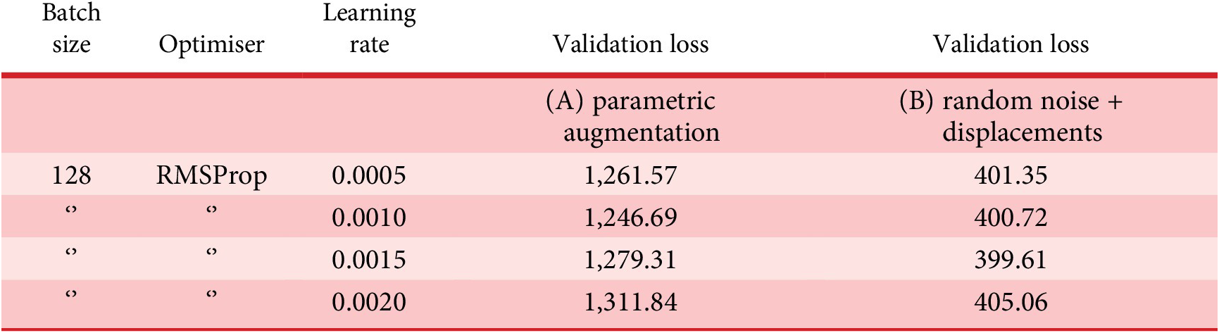
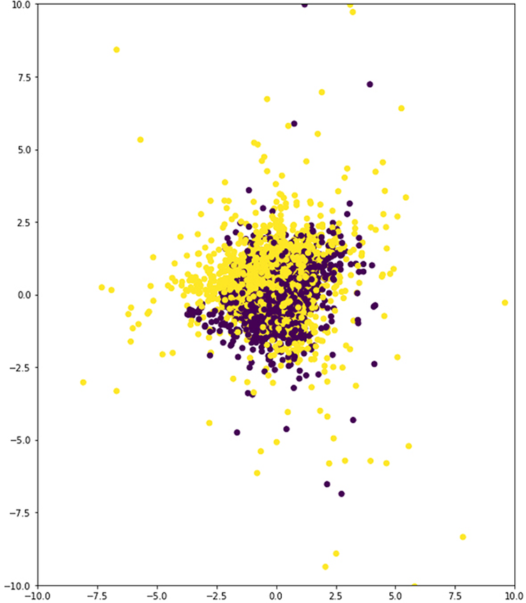
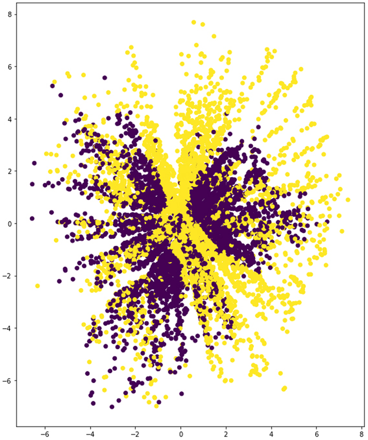
In the case of the displacement and noise data set, training yields much lower error rates than parametric augmentation (Table 2, Table 3 and Figure 12). This is understandable, as the spectrum of geometries enabled by the new method is much more diverse and, thus, requires stronger learning capabilities from the VAE model. However, the latent space resulting from the latter shows that the network is already able to differentiate the two building types to some extent (Figure 13a), whereas the latent space corresponding to the former is far from capable of rendering this distinction (Figure 14). Additionally, there are distinct structural features that can be observed in the latent space corresponding to the parametric augmentation data set (Figure 13b), which are not present in any form in the other latent space. Finally, in Figure 13a, the VAE was able to spread out the samples taking a broader portion of the latent space than in Figure 14, where most samples are concentrated in between the values (−2.5, 2.5) on the vertical axis. While these are purely visual observations, it is advisable to approach this analysis from a more rigorous methodology in future work, especially in cases where the distinction is less obvious.
Hyperparameters and results of preliminary experiments
Training results for preliminary experiments

Best training results for both the parametric augmentation data set and the previous random displacements + noise data set.

Latent space. Encoded samples from the parametric augmentation data set (yellow and purple dots represent each of the two training categories).
Highlight of observed structural features in the latent space from the parametric augmentation data set.
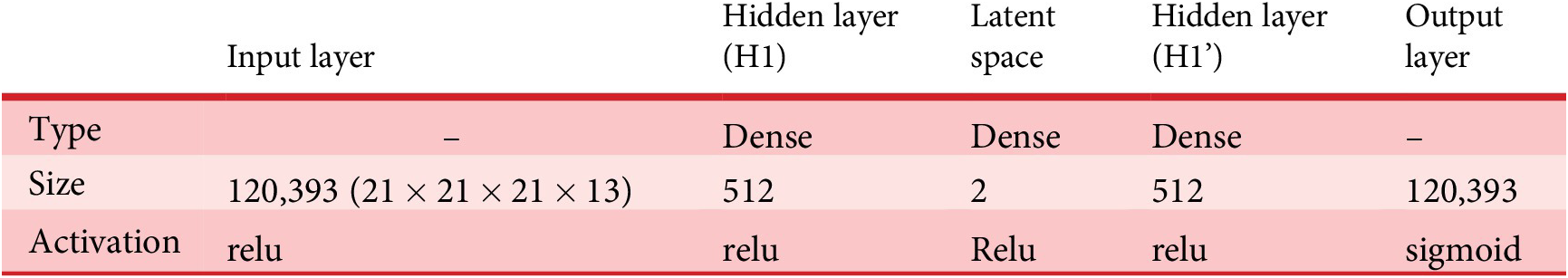
Latent space. Encoded samples from the random displacements + noise data set.
A plausible interpretation of this apparent contradiction would point to the possibility that the variety of the information contained in the data set generated through random discrete displacements (which are very limited in comparison with the volume of the data set) and random noise in the values of the connectivity vector is not rich enough to enable the learning of relevant features. If the network learns features that are not representative of the inputs, it may not be able to separate them on a latent space even if it succeeds in reconstructing them. Accordingly, it is concluded that the data set produced through parametric augmentation offers better prospects for further training. It must be noted, though, that there is a distinctive feature that clearly differentiates the two types: the CCTV has no diagonal elements. This may give the VAE a head start in the training process in terms of separating both classes in the latent space. In order to test for generality, more types should be scrutinised. However, this early work attempts only to carry out an initial exploration on the potential of the methodology presented here.
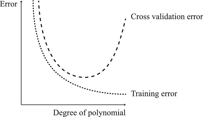
Upon proof of the potential benefits of the aforementioned parametric augmentation strategy, the second set of experiments attempts to establish whether a network architecture based on 3D convolutional hidden layers would outperform a model containing only linear layers that are densely connected. Convolutional layers can help to keep the number of trainable parameters in check, as will be explained in the discussion of results. This is important because if the ratio to the number of training samples is overweighed by the parameters, then there is a very high risk of overfitting. Deep architectures can be extremely powerful; however, there is a trade-off between the magnitude of the problems that a neural network can solve and the overfitting of the network to the data, as shown in Figure 15.
Model complexity versus training and validation errors (overfitting problem).
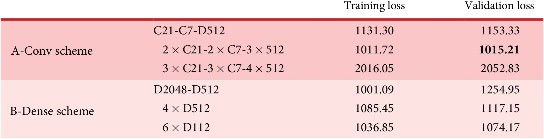
For this set of experiments, two groups of network architectures have been selected upon further preliminary testing. The first group (A-Conv) includes three convolutional schemes and the second (B-Dense), three standard feed-forward configurations with varying numbers and sizes of hidden layers. The first model (C21-C7-D512) of the A-Conv group features two 3D convolutional layers in the encoder, leading to a linear dense layer of 512 neurons and a symmetrical decoder. Latent space is again 2D (and will remain the same in all the experiments). The first of the layers is a 3D convolutional layer arranged spatially as 21 × 21 × 21 neurons with a depth of 13 channels. Convolutions are applied in 3 × 3 × 3 units with maximum overlap. The size of the second one is 7 × 7 × 7, and the rest of the configuration remains identical. The second model (2 × C21−2 × C7-3 × D512) duplicates both convolutional layers and adds two more dense layers of 512 neurons at the end and beginning of the encoder and decoder, respectively. Repetition of convolutional layers has delivered good results when applied to deep neural networks (Simonyan & Zisserman Reference Simonyan and Zisserman2015). Finally, the third model (3 × C21-3 × C7-4 × D512) adds another convolutional layer in between each of the two pairs of convolutional layers of the previous model. Both these new layers feature an increased depth of 39 channels. Also, at the end of the encoder, an additional dense layer is allocated maintaining the same configuration of the three preceding layers. The decoder as always is the exact mirror. The three architectures described above contain 982 k, 5.78 M and 6.725 M trainable parameters, respectively. For each one, different learning rates have been tested, and the final configuration is shown in Tables 4a–c. Training results for the A-Conv set are shown in Figure 16.
C21-C7-D512 network architecture (showing only encoder for simplicity)
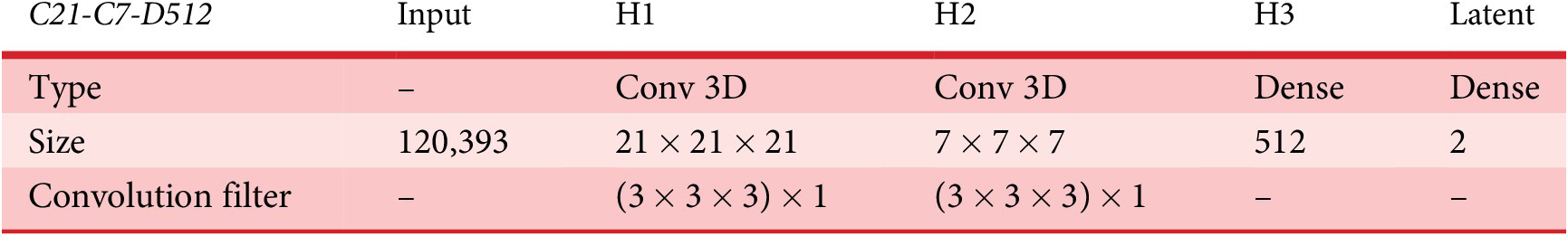
Notes: Optimizer RMSProp, Lr (learning rate) = 0.0017, Stride = 1
All activations are ReLu except output layer (sigmoid)
Total parameters: 982 k
2xC21-2 × C7-3 × D512 network architecture (showing only encoder for simplicity)
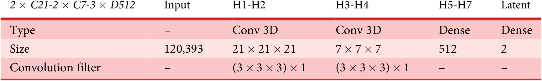
Notes: Optimizer RMSProp, Lr = 0.0011, Stride = 1
All activations are ReLu except output layer (sigmoid)
Total parameters: 5.78 M
3 × C21-3 × C7-4 × D512 network architecture (showing only encoder for simplicity)
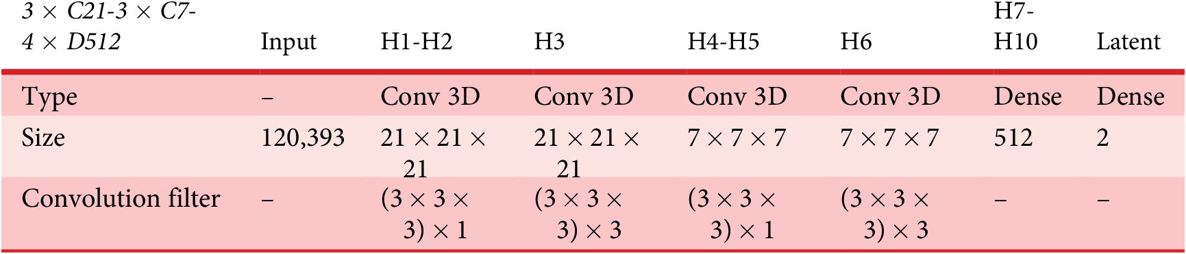
Notes: Optimizer RMSProp, Lr = 0.0009, Stride = 1
All activations are ReLu except output layer (sigmoid)
Total parameters: 6.72 M
Best training results of A-Conv scheme.

In the B-Dense group (Tables 5a–c), the first model (D2048-D512) bears two hidden layers that are densely connected for both encoder and decoder. The first hidden layer holds 2048 neurons and the second one 512, which amount to 495.35 M trainable parameters. In the second model (4xD512), these two hidden layers are replaced by four identical hidden layers of 512 neurons, thus reducing the parameter count to 125.245 M. This value, however, may still be quite high for the data set at hand. Finally, a third model (6 × D112) is set up containing up to six hidden layers of 112 neurons each, both in the encoder and decoder. This last model cuts the total parameter count down to 27.215 M, which is still a remarkable figure, nonetheless. Training results for the B-Dense scheme are shown in Figure 17.
D2048-D512 network architecture (showing only encoder for simplicity)
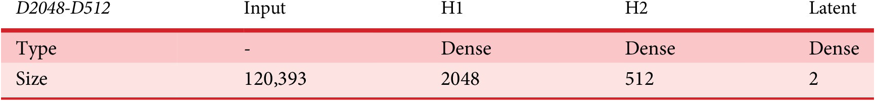
Notes: Optimiser RMSProp, Lr = 0.0012
All activations are ReLu except output layer (sigmoid)
Total parameters: 495.35 M
4 × D512 network architecture (showing only encoder for simplicity)
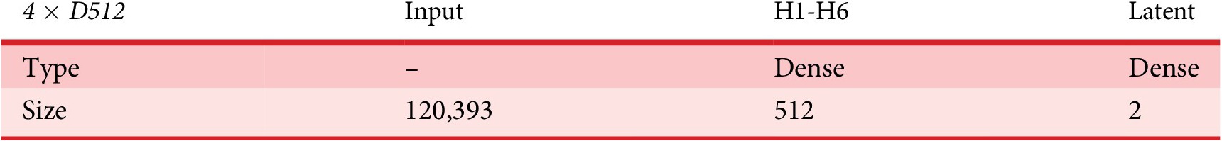
Notes: Optimiser RMSProp, Lr = 0.0015
All activations are ReLu except output layer (sigmoid)
Total parameters: 125.24 M
6 × D112 network architecture (showing only encoder for simplicity)

Notes: Optimiser RMSProp, Lr = 0.0010
All activations are ReLu except output layer (sigmoid)
Total parameters: 27.21 M
Best training results of B-Dense scheme.

The best performing architectures from each scheme are 2 × C21-2 × C7-3 × D512 and 6 × D112. The first one features a total of four convolutional hidden layers and three hidden dense layers for both encoder and decoder. The second model is composed of six dense layers in between the input and the latent space, and the same layers again in between the latent space and the output layer of the autoencoder. The performance of both models in terms of validation loss is relatively similar as can be seen in Table 6 and Figures 16 and 17. However, the latent spaces that each of these two architectures present are quite different (Figures 18 and 19). The convolutional scheme in fact enables a more structured differentiation of the two categories present in the input data set. It is expected that a network performing satisfactory pattern recognition is also able to learn relevant features from each geometric type, leading to successful 3D form interpolations.
Training results for A-Conv and B-Dense schemes
Latent space of 2 × C-2 × C-3 × D512 model.

Latent space of 6 × D112 model.
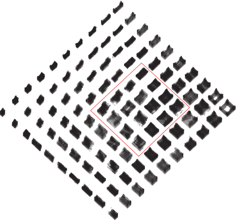
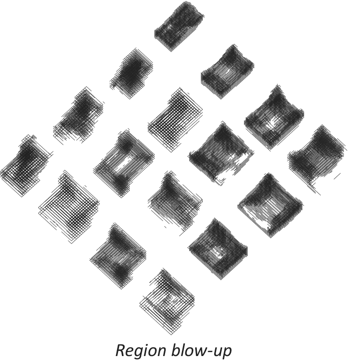
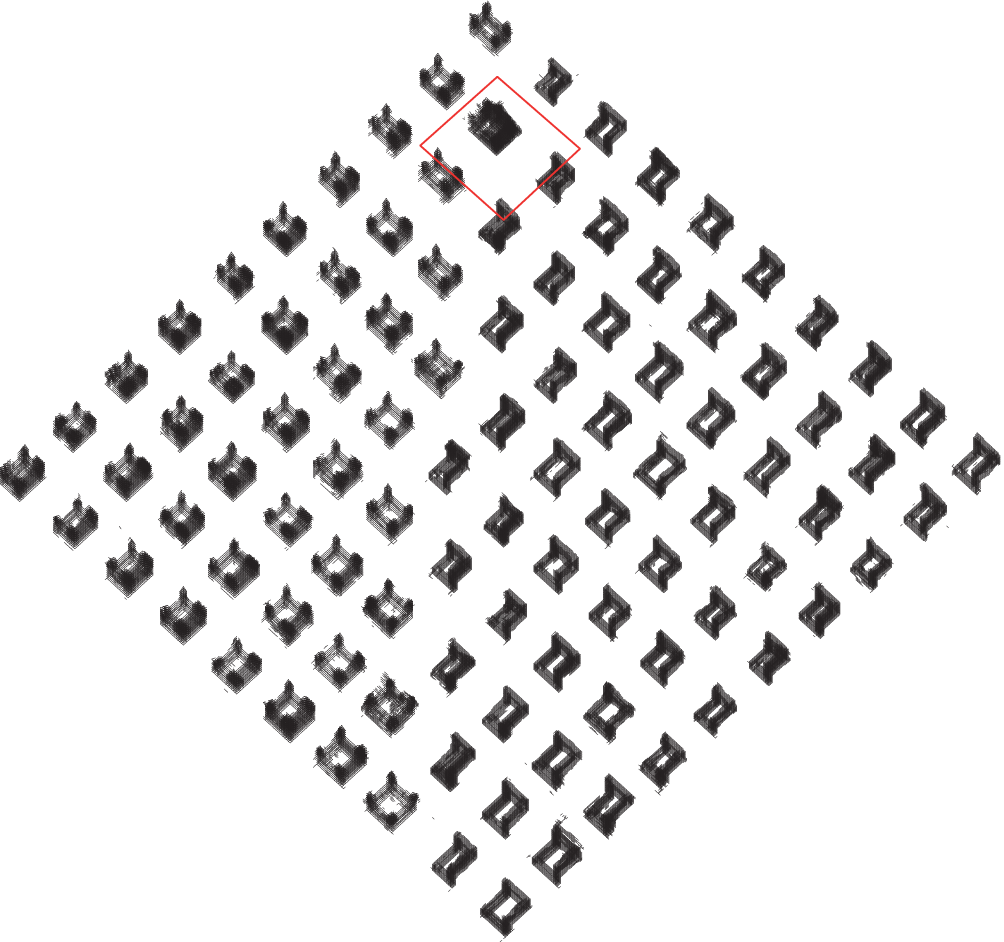
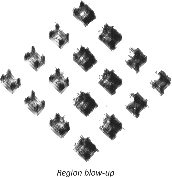
The reconstructed geometries resulting upon sampling a grid of 10 × 10 points from the latent space through the decoder are shown in Figure 20–23 for both models. The model from convolutional scheme exhibits a smooth transition across this space, whereas the dense architecture selected presents less structured variations of geometry. However, both lack capacity to produce well-defined structures, in the sense that the reconstructed geometries are somewhat blurry.
Geometry reconstructed from latent space. Model 2 × C-2 × C-3 × D512.
Geometry reconstructed from latent space (blow-up). Model 2 × C-2 × C-3 × D512.
Geometry reconstructed from latent space. Model 6 × D112.

Geometry reconstructed from latent space (blow-up). Model 6 × D112.

This second set of tests aimed at finding a network architecture capable of clearly differentiating the two types present in the data set. As explained earlier, more powerful architectures may lead to overfitting issues if the size of the data set does not tally up with the complexity of the model. For this reason, these experiments targeted the use of convolutions in hidden layers. When there are patterns relating to spatial relationships in the samples of a data set, the use of convolutional layers can be more efficient than standard densely interconnected layers, as they provide a means to reduce the number of trainable parameters of the model while maintaining a strong learning capacity (Simonyan & Zisserman Reference Simonyan and Zisserman2015). In Figure 17, results show that the first dense model (D2048-D512) achieves the best training loss values but clearly over fits after a few training epochs, which is not surprising since it has 495.35 M parameters to adjust. The second dense model (4 × D512) starts to over fit slightly after 20 epochs and presents strong convergence instability. The third and last of the dense models is the best performing among the dense schemes (B-Dense). It only over fits moderately after 30–40 epochs and achieves validation loss values comparable to the best of the convolutional scheme (A-Conv). However, this model presents very high convergence stability, which is not reflected in the graph but was apparent during testing; it took several failed runs until the network actually converged. In Figure 16, the best performing model from A-Conv (2 × C21-2 × C7-3 × D512) presented a more stable behaviour and slightly outperformed all the models of B-Dense in terms of validation loss. This model achieves a better score than the other two in its group because of its balance in complexity; deeper models like 3 × C21-3 × C7-4 × D512 are fit for such level of complexity that they require much more massive data sets to feed on; while on the other side of the spectrum, the model C21-C7-D512 is too simple to deal with the current data set.
Although the best performing models from each scheme present similar validation loss values, they behave very differently in the way they encode input samples into the latent space. Results in Figures 18 and 19 show very different spatial distributions for each model. Specifically, the convolutional model displays a very structured distribution, including the particularity of a sort of ‘nesting rings’ formation that suggests the need of adding a third dimension to the latent space to enable continuity among the encoded samples of each category (which may be explored in future work). The latent space of the dense model, on the contrary, displays a less structured distribution and a lower spatial capacity to segregate categories. This is an interesting finding that might be connected to the fact that convolutions are especially well-suited for spatial data. As a result, the geometries being sampled anew from the latent space through the decoder present smoother interpolation gradient in the convolutional model than in the dense counterpart (Figures 20–23).
Despite achieving smooth transitions, the reconstruction error reported in the results is too high. This underperformance causes the new geometries to appear blurry, which completely defeats the purpose of representing geometry as connectivity maps. The original motivation behind this representation of structural types was to move away from pixel- or voxel-based approaches that were rooted in extensive developments in computer vision. Thus, obtaining outputs that resemble voxelised geometries are not satisfactory.
The last round of experiments attempts to reduce the blur effect present in the reconstructed geometries. In this test, the 2 × C21-2 × C7-3 × D512 network model was employed since it had delivered the best results so far. The objective is to further reduce the values of validation loss, thus improving the definition of the output geometry. To achieve this target, two strategies are implemented. The first one consists simply of providing a larger data set. To this end, a new data set is generated containing 75 k samples for each of the two working types. The second strategy focusses on reducing the learning problem that the VAE faces. This has been carried out by limiting the value ranges of the parameters that generate the training samples. Furthermore, this limitation has been conducted in a way that allows for a number of unique variations that match exactly the total number of desired samples in this data set. In this way, it is expected that the input geometries suffer the least variations possible, while each sample remains strictly unique (and thus all samples provide new information that can be learned by the network). In particular, the parameters that have been most limited are width and length. Previously, these two dimensions were free to take up the complete size of the canvas, whereas in the restricted data set, they do not exceed half the length or width of the canvas. These two strategies have been tested through two experiments. In the first one, the data set is increased and nothing else is altered, and in the second one, the data set is increased and a limit to the variation of the parametric augmentation method has been applied as explained above. The results of these experiments are shown in Table 7 and Figures 24–28. The data show a large reduction in validation loss (50%) and a latent space with a very clear pattern segregation. It can also be observed that interpolation of geometry takes place along a very narrow passage in between the two clusters. A detailed visualisation of the output geometry for the second case (modified and increased data set) is shown in Figures 29 and 30.
Training results for 2 × C21-2 × C7-3 × 512 upon variations of the data set

Latent space of 2 × C21-2 × C7-3 × D512 model with the ‘increased data set’.
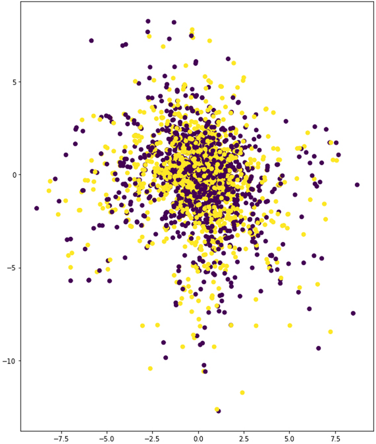
Latent space of 2 × C21-2 × C7-3 × D512 model with the ‘modified and increased data set’.

Comparison of training results of 2 × C21-2 × C7-3 × D512 model from the previous experiment with both the ‘increased data set’ and the ‘increased and modified data set’.

Geometry reconstructed from latent space. Model 2 × C-2 × C-3 × D512 using the increased and modified data set.
Geometry reconstructed from latent space (blow-up). Model 2 × C-2 × C-3 × D512 using the increased and modified data set.
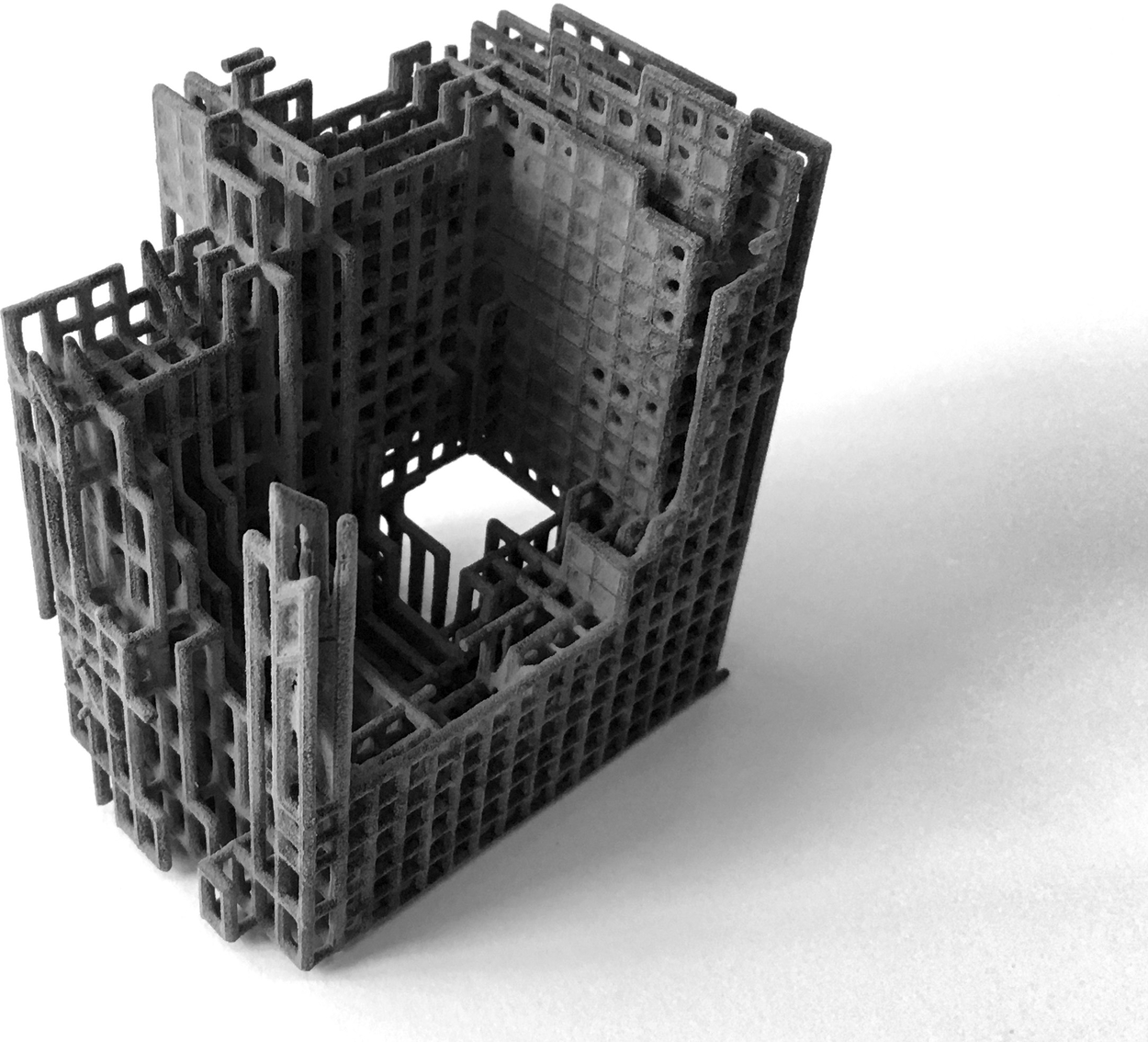
Rendered geometry reconstructed from latent space. Model 2 × C-2 × C-3 × D512 using the increased and modified data set.

3D printed geometry reconstructed from latent space. Model 2 × C-2 × C-3 × D512 using the increased and modified data set.
These last two experiments were an attempt to bring down reconstruction error by providing a larger data set and limiting the range of variations of the samples that are generated through parametric augmentation. In Figure 20, it can be observed that a great part of the transition gradient deals mostly with accommodating variations in size, rather than picking up morphological or topological features, which are central to this study. Thus, the motivation behind reducing parameter variation ranges such as those applied to the width and length of the samples responds to the intention of improving the network’s accuracy by eliminating unnecessary information that leads to no relevant learning.
In the first of these two experiments, the parameters for generation of samples through parametric augmentation remained unchanged. However, the size of the data set was more than doubled. In Figure 24, the latent space corresponding to this test reveals that the model was totally incapable of separating the two types. The experiment thus suggests that increasing the number of training samples does not provide the network with better learning prospects. This finding is rather interesting because the initial objective of using parametric augmentation was precisely to afford the possibility of generating large data sets as required by the complexity of the problem at hand. However, this result shows exactly the opposite: when the variations achieved through parametric augmentation are too broad, the shear scope of these may easily surpass the hypothetical benefit of providing more samples. In the second experiment, the parameters guiding these variations were heavily restricted with the intention of producing less heterogeneity while still generating the desired number of unique samples. Results (Figures 27 and 28) prove the strategy effective in bringing down validation loss roughly around 50%, which is highly successful. Additionally, categories are clearly separated after encoding. However, the resultant latent space (Figure 24) shows a hard fault line in between the two training categories. This condition entails that interpolation of geometry may only happen in a very narrow area, and that transitions will not be able to display smooth gradients. In Figure 27, this effect can be clearly observed in the distribution of the generated geometries, and the region blow-up effectively reveals abrupt transitions along the fault line.
It is unclear at this stage the reason behind this fallback into unsatisfactory interpolation spaces, especially despite the positive results in terms of both validation loss and spatial segregation in the latent space. Possible explanations may be connected to the particular geometries selected for the experiments, in the sense that they may not share common distinctive features that allow clean interpolations. Or perhaps, the network architectures implemented in this work lack ability to capture global features from one or both input types. Finally, there is another possible factor that should be mentioned, one that touches upon the core of the methodology presented here and that should be taken into consideration for future work. Machine learning algorithms are essentially optimisation models. Most of them function based on the gradient descent, whereby a relevant local minimum of the loss function may be found. However, loss functions must be continuous and tractable and should not present frequent or large areas of null derivative (plateaus). If these areas are prevalent in the function, then the algorithm may not know in which direction to move when pursuing lower loss values. It may assume that it has already touched bottom, or it may trigger a random decision regarding which direction to take, resulting in high volatility during the training process (as can be seen in Figures 17 and 26) and low convergence. In fact, models that did not converge easily have been prominently present throughout much of the side work carried out during the present study. The alternative representation of geometry that has been put forward here is based on a connectivity vector of discrete values (0, 1). Additionally, in this last experiment, variations among the training samples were minimised to avoid an excessive spread of features. This means that many samples shared large sets of identical values, facilitating the emergence of flat areas in the loss function. And where those values were different, a transition pattern was hard to find due to the discrete nature of the representation method chosen to approach the problem. It may thus be valuable when engaging in further work to look into some valuable research that is currently taking place to tackle deep learning problems in discrete spaces. Works along the lines of (Hafner et al. Reference Hafner, Lillicrap, Fischer, Villegas, Ha, Lee and Davidson2018; Gouk et al. Reference Gouk, Frank, Pfahringer and Cree2018) attempt to find alternative representations of these spaces that smooth out the issues mentioned above. The adoption of the methods proposed in these studies may provide the answers that are required to improve the results presented in this paper.
5. Conclusions
Due to the growing international academic interest in generative machine learning methods and its wide commercial applications, the workflow presented in this paper builds on the emergence of a burgeoning field. Although developed five years ago, the use and usefulness of VAEs in the context of architectural design remains mostly unexplored.
The work presented in this paper builds on the notion of a connectivity vector that is used to represent 3D mesh-like geometries, with the objective of facilitating their processing by neural networks in general and VAEs in particular. This representation was explored in (de Miguel et al. Reference de Miguel-Rodriguez, Villafañe, Piškorec and Sancho-Caparrini2019), where a data set comprising two building types was generated through noise and displacement-based augmentation. The results suggested on the one hand, that noise did not help the network in identifying patterns. And on the other hand, that the displacement approach was always prone to overfitting, because the larger the displacement space, the more the number of trainable parameters grew. In this context, the main objective of the present work has been to explore the suitability of an alternative augmentation method in assisting the generation of novel geometries with a VAE.
This alternative method, parametric augmentation, has allowed very large data sets to be created without the need to increase the size of the 3D-canvas (and consequently the size of the input layer and total number of trainable parameters), as was the case in the previous approach. Additionally, parametric augmentation is particularly efficient for increasing data sets of 3D geometries within the field of architectural geometry – especially when resembling building types, due to the discrete yet observable characteristics of each sample, as constituent of each type. The results presented in this paper show that the method was indeed successful in preventing the original overfitting problem. Consequently, the autoencoder was successful in reconstructing the geometries of the data set. The augmentation method, however, has posed another set of problems that have challenged the performance of the VAE.
Firstly, results show that the feature spread produced through parametric augmentation can overwhelm the network and can hinder its ability to extract those features. This was made apparent when an increase in the size of the data set worsened the reconstruction error rather than improving it. This limitation blocked the possibility of expanding the data set to improve the definition of the geometries being generated by sampling from the latent space. Thus, although there were smooth transitions across the two types present in the resulting geometries, these remained quite blurry. Secondly, when attempting to counter the latter issue by limiting the range of the parameters involved in building up the training set, it was found that despite being effective in further lowering the reconstruction error, transitions across types had been drastically reduced.
An important takeaway from the experimentation is that there seems to be a more fundamental problem underlying the difficulties faced by the VAE. As discussed in the previous section, the representation based on a connectivity vector as implemented in this study brings about a tough landscape to be navigated by optimisation algorithms. This is mainly due to the discrete and sparse nature of the data set. Potential avenues of research that may shed light onto this problem touch upon transformation techniques from discrete spaces into continuous ones. Some of these have been indicated in this paper for future work, as they are currently being pursued by several authors. Despite the difficulties, the final results show a partial success in generating new geometries from the latent space that share a mix of features from the two types present in the training set, which was the initial objective of the research. The quality of these new samples achieves a certain degree of interpolation as can be observed in Figures 29 and 30, although the definition of the resulting geometries may still be improved.
Aside from the definition of the results, the main contribution of this paper has been to explore an alternative avenue for the parametric generation of large data sets of 3D geometries, showcasing its problems and limitations in the context of neural networks and VAEs and pointing out potential solutions for future work. Overall, the proposed workflow challenges designers to acquire a critical perspective of the impact and potential of AI in our society and design practices. Generative neural network models have a large potential to redefine how architects and designers work with architectural precedents, namely, to use them directly as data for design generation. The work presented in this paper aims to show the potential of such techniques and open a discussion about the future of machine learning in the context of geometry generation for the architectural design industry.


 Open access