


I. Introduction
A growing literature examines how corporate environmental behavior can be influenced by various stakeholders, such as equity investors (Akey and Appel (Reference Akey and Appel2019), Kim, Wan, Wang, and Yang (Reference Kim, Wan, Wang and Yang2019), and Bellon (Reference Bellon2025)), financial analysts (Jing, Keasey, Lim, and Xu (Reference Jing, Keasey, Lim and Xu2024)), local media (Heese, Pérez-Cavazos, and Peter (Reference Heese, Pérez-Cavazos and Peter2022)), banks (Bellon (Reference Bellon2021)), and social rating agencies (Chatterji and Toffel (Reference Chatterji and Toffel2010)). Among various monitoring forces, the government represents a formal institution that profoundly impacts firms’ environmental policies through regulatory oversight (e.g., the Environmental Protection Agency (EPA)) and environmental regulations (e.g., the Clean Air Act) (Gray and Shimshack (Reference Gray and Shimshack2011)).Footnote 1 Importantly, government agencies can act as customers and constitute a pivotal part of the U.S. economy.Footnote 2 While the implications of government procurement for corporate outcomes have attracted widespread attention from the public, media, and policymakers (Cohen, Li, Li, and Lou (Reference Cohen, Li, Li and Lou2022)), little is known about the role of the government as a customer in shaping corporate environmental policies. We fill this gap by investigating how government procurement affects a firm’s toxic pollution.
Government customers, including agencies and departments that purchase on behalf of the federal government, have strong incentives to monitor corporate environmental policies. They are required by various federal regulations to achieve sustainable procurement with a particular focus on reducing the toxic pollution of their contractors (i.e., suppliers). Specifically, Federal Acquisition Regulation (FAR) Part 23 promotes sustainable acquisition by requiring federal agencies to prioritize products and services that reduce risks to human health and the environment, particularly those related to toxic pollution. Contractors are subject to standards that emphasize pollution prevention, the safe handling of hazardous materials, and the use of environmentally preferable products. Additionally, under FAR Part 52, contractors may be required to implement programs to reduce waste and toxic substances, as specified in their contracts. Executive Order 12969, issued by President Clinton in 1995, requires government contractors to comply with toxic chemical release reporting requirements throughout the contract duration (see https://www.govinfo.gov/content/pkg/FR-1995-08-10/pdf/95-19972.pdf). According to FAR Part 42, environmental compliance is evaluated through the Contract Performance Assessment Reporting System, and contracting officers are responsible for monitoring “the contractor’s environmental practices for adverse impact on contract performance or contract cost, and for compliance with environmental requirements specified in the contract.”Footnote 3
From a contractor’s perspective, violating federal contractual requirements likely leads to more severe losses than violating private-sector contractual requirements (Engstrom (Reference Engstrom2012)), suggesting higher ex ante expected costs of violations in the presence of government customers. When the government detects a contractor’s noncompliance, it may initiate a lawsuit that entails monetary penalties and impose stricter contract terms (Heese and Pérez‐Cavazos (Reference Heese and Pérez‐Cavazos2019), Samuels (Reference Samuels2021), Cohen et al. (Reference Cohen, Li, Li and Lou2022)). Contractors with poor environmental performance are considered irresponsible, potentially leading to suspension or termination of government business relationships. To promote accountability, the government formally discloses environmental violations and procurement-related sanctions through enforcement actions, particularly under the False Claims Act. For instance, in 2016, Lockheed Martin paid a 5-million-USD penalty to settle allegations of violating hazardous waste laws and knowingly submitting false claims to the Department of Energy. The company was accused of misrepresenting its compliance with the Resource Conservation and Recovery Act and failing to properly manage, report, and dispose of hazardous waste (see https://www.justice.gov/opa/pr/lockheed-martin-agrees-pay-5-million-settle-alleged-violations-false-claims-act-and-resource). Such enforcement outcomes are often publicized through the Department of Justice press releases and official reports. Penalties and public disclosure serve as a deterrent to potential violators and reinforce the government’s commitment to environmental sustainability. Thus, we hypothesize that contractor firms under government scrutiny are incentivized to improve their environmental performance to avoid the severe consequences of environmental misbehavior.
To estimate the effect of government customers on corporate environmental policies, we obtain federal government contract data from the USAspending.gov website. Following prior studies (e.g., Mills, Nutter, and Schwab (Reference Mills, Nutter and Schwab2013), Hadley (Reference Hadley2019), and Samuels (Reference Samuels2021)), we measure government contracting by the number of a firm’s federal government contracts in a year and the ratio of total contract value to firm sales in a year. To measure corporate toxic pollution, we use Toxics Release Inventory (TRI) data on the amount of toxic emissions released by the registered plants of U.S. firms. Our final sample consists of 9,438 firm-year observations for 793 unique public firms (with at least one plant in the TRI database) over the period of 2001–2019. We find that government contractor firms have significantly lower levels of toxic pollution. Specifically, a 1% increase in the number of government contracts is associated with a 0.086% and 0.091% decrease in the total toxic pollution and sales-scaled toxic emissions of contractor firms, respectively. The results hold across a comprehensive set of robustness tests, providing strong support for our hypothesis that monitoring by government customers significantly reduces corporate pollution.
To substantiate the argument that government customers play an external governance role in reducing corporate pollution, we perform cross-sectional analyses. First, the negative effect of government customers on corporate pollution is stronger for firms with longer-duration contracts, echoing the view that more interactions between the government and its contractors over longer contracting horizons facilitate monitoring. Furthermore, government customers have a greater effect on corporate pollution reduction for firms that rely more on government contracts and for firms without political connections, because such firms are more incentivized to maintain business relationships with government customers. Collectively, the cross-sectional evidence suggests that the mitigating effect on pollution is, on average, more than twice as large in subsets of firms facing greater government scrutiny, highlighting the monitoring role of government customers in curbing supplier pollution.
However, the relationship between having government customers and corporate environmental policies could be spurious. Unobserved heterogeneity correlated with both government contracting and corporate environmental policies could bias the results. To allay potential endogeneity concerns, following prior studies (Cohen, Coval, and Malloy (Reference Cohen, Coval and Malloy2011), Cohen and Malloy (Reference Cohen and Malloy2016), Kong (Reference Kong2020), and Cohen et al. (Reference Cohen, Li, Li and Lou2022)), we use turnovers in congressional committee chairmanships as an exogenous shock to state-level federal government expenditures. The rationale is that government procurement often experiences a substantial increase for firms headquartered in states represented by a new powerful chair (Cohen et al. (Reference Cohen, Coval and Malloy2011)). Our difference-in-differences (DiD) analysis provides consistent evidence that suppliers experiencing a plausibly exogenous increase in federal government procurement significantly reduce corporate pollution. Specifically, congressional chairman turnovers are associated with a 29.7% reduction in both the total toxic pollution and sales-scaled toxic emissions of treated firms, relative to control firms.
Next, we explore two channels through which government customers shape their contractor firms’ environmental policies. The first channel pertains to internal environmental governance, with a particular focus on building human capital through the appointment of sustainability directors and the provision of environmental training to employees. We find that, on average, a 1-unit increase in the sales-scaled value of government contracts is associated with a 1.26 percentage point increase in the likelihood of appointing a sustainability director and a 3.35 percentage point increase in the likelihood of providing environmental management training, respectively. The second channel is more direct as it focuses on firm pollution abatement investments aimed at preventing pollution at its source. Our analysis shows that a 1-unit increase in the sales-scaled value of government contracts is associated with a 2.18 percentage point higher likelihood of making environmental investments, and with a 0.95 and 0.78 percentage point higher likelihood of investing in operations-related and production-related pollution prevention practices, respectively. Moreover, the corresponding DiD analyses based on congressional chairman turnovers provide largely consistent evidence. The DiD results indicate that turnovers are associated with increases of 10.6 percentage points in the likelihood of environmental management training, 11.67 in environmental investments, 6.67 in operations-related pollution prevention investments, and 7.95 in production-related pollution prevention investments among treated firms, relative to control firms.
Further, we assess two alternative explanations for our findings. First, we examine whether the lower pollution in government contractor firms is driven by a reduction in firms’ economic activities. The results provide little support for this conjecture. Using production volume and employment growth as proxies for economic activities (Akey and Appel (Reference Akey and Appel2021)), the relationship between government customers and overall firm economic activities is statistically insignificant. Second, we consider whether government contracting alleviates the financial constraints of contractor firms, thereby allowing more investment in pollution abatement. Inconsistent with this explanation, we observe an insignificant effect of government customers on their contractors’ financial constraints. Ruling out these alternative explanations reinforces our interpretation that the external governance provided by government customers shapes corporate environmental policies and performance.
In the final part of our analysis, we explore the consequences of firm environmental misbehavior. While our main analysis focuses on the government’s ex post monitoring role, environmental performance may influence the ex ante selection of contractors (Flammer (Reference Flammer2018)). We test this ex ante effect by examining the impact of firms’ environmental violations on procurement outcomes. We find that environmental violations in the past 5 years significantly reduce both the number and value of government contracts awarded to violators, suggesting that government customers consider environmental records when selecting suppliers. In addition, our analysis of corporate pollution around first-time government contract awards (Samuels (Reference Samuels2021)) confirms the presence of both ex ante selection and ex post monitoring effects. Taken together, our study reveals that government customers promote corporate environmental sustainability through both selection and monitoring.
Our article makes two main contributions. First, it adds to the literature on the determinants of corporate environmental policies. One line of this research focuses on various corporate and managerial characteristics, such as organizational form (Akey and Appel (Reference Akey and Appel2021)), financing capacity (Cohn and Deryugina (Reference Cohn and Deryugina2018), Levine, Lin, Wang, and Xie (Reference Levine, Lin, Wang and Xie2018), Xu and Kim (Reference Xu and Kim2022), and Bartram, Hou, and Kim (Reference Bartram, Hou and Kim2022)), executive incentives (Berrone and Gomez-Mejia (Reference Berrone and Gomez-Mejia2009), Flammer, Hong, and Minor (Reference Flammer, Hong and Minor2019)), ownership structure (Berrone, Cruz, Gomez-Mejia, and Larraza-Kintana (Reference Berrone, Cruz, Gomez-Mejia and Larraza-Kintana2010), Shive and Forster (Reference Shive and Forster2020)), and segment disclosure (Jing, Xu, and Zuo (Reference Jing, Xu and Zuo2025)). More relevant to us, another line of research explores the roles of various stakeholders, including local institutional investors (Kim et al. (Reference Kim, Wan, Wang and Yang2019)), hedge funds (Akey and Appel (Reference Akey and Appel2019), Chu and Zhao (Reference Chu and Zhao2019), Naaraayanan, Sachdeva, and Sharma (Reference Naaraayanan, Sachdeva and Sharma2021)), private equity (Bellon (Reference Bellon2025)), financial analysts (Jing et al. (Reference Jing, Keasey, Lim and Xu2024)), banks (Bellon (Reference Bellon2021)), corporate customers (Chen, Su, Tian, Xu, and Zuo (Reference Chen, Su, Tian, Xu and Zuo2025)), and local media (Heese et al. (Reference Heese, Pérez-Cavazos and Peter2022)). Our study sheds light on this inquiry by highlighting the important role of government customers in determining corporate environmental policies.
Second, our article contributes to the literature on the microeconomic outcomes of government spending.Footnote 4 The extant literature on the real effects of government procurement shows that government contractors tend to have favorable loan contract terms (Cohen et al. (Reference Cohen, Li, Li and Lou2022)), higher stability and profitability (Goldman (Reference Goldman2020), Cohen and Li (Reference Cohen and Li2020)), less corporate innovation (Kong (Reference Kong2020)), and a lower cost of equity (Dhaliwal, Judd, Serfling, and Shaikh (Reference Dhaliwal, Judd, Serfling and Shaikh2016)). A closely related strand of literature exploring the implications of government customers’ monitoring of their contractors shows that such monitoring helps enhance contractors’ financial reporting quality and transparency (Samuels (Reference Samuels2021)) and reduces federal tax avoidance (Mills et al. (Reference Mills, Nutter and Schwab2013)). Complementing these studies, we document an important and underexplored impact of government spending on corporate environmental policies: government monitoring significantly improves the supplier firm’s environmental performance and reduces its environmentally irresponsible behavior.
II. Data, Empirical Model, and Descriptive Statistics
A. Pollution Data
We obtain data on corporate pollution from the TRI database of the EPA. The database has been widely used in previous literature to assess corporate environmental performance (e.g., Klassen and McLaughlin (Reference Klassen and McLaughlin1996), King and Lenox (Reference King and Lenox2002), Berrone et al. (Reference Berrone, Cruz, Gomez-Mejia and Larraza-Kintana2010), Akey and Appel (Reference Akey and Appel2021), Xu and Kim (Reference Xu and Kim2022), Hsu, Li, and Tsou (Reference Hsu, Li and Tsou2023)). Since 1987, the TRI program has required U.S. plants to report toxic emissions information if a facility: i) manufactures, processes, or uses 1 of over 700 TRI-listed chemicals; ii) has 10 or more full-time employees; and iii) operates in 1 of the approximately 400 industries covered by the program.Footnote 5 One unique feature of the TRI database is that it provides detailed information on plants with toxic emissions, including facility name, parent company name, reporting year, and the quantity of toxic pollution released into the environment.
We supplement the TRI data with the financial information of U.S. public firms from the Compustat database. Since there is no common identifier for firms across the two data sets, following previous studies (e.g., Akey and Appel (Reference Akey and Appel2019), Akey and Appel (Reference Akey and Appel2021), Xu and Kim (Reference Xu and Kim2022), and Jing et al. (Reference Jing, Keasey, Lim and Xu2024)), we conduct both fuzzy matching and manual checks. Specifically, we first apply a fuzzy string-matching algorithm to match the parent company names in the TRI database with the company names in Compustat. We then manually check the matched firms based on company address, company website, and the DUNS number to ensure matching accuracy.Footnote 6 Following Akey and Appel (Reference Akey and Appel2019), (Reference Akey and Appel2021) and Chu and Zhao (Reference Chu and Zhao2019), we exclude plants with zero toxic pollution. This procedure leaves us with 6,918 plants across 793 unique firms over the period of 2001–2019.Footnote 7 Since the explanatory variables are lagged by 1 year relative to the firm-level pollution variables in our main analysis, the pollution data span from 2002 to 2020.
The toxic emissions data from the TRI data set are at the chemical-facility-year level. To capture a firm’s environmental performance, we aggregate the amount of all chemical emissions across its facilities to construct two firm-level measures of toxic pollution (e.g., Chatterji and Toffel (Reference Chatterji and Toffel2010), Chu and Zhao (Reference Chu and Zhao2019), Bartram et al. (Reference Bartram, Hou and Kim2022), and Jing et al. (Reference Jing, Keasey, Lim and Xu2024)). LN(POLLUTION) is the natural logarithm of toxic pollution. LN(POLLUTION/SALES) is the natural logarithm of toxic pollution scaled by total sales. One justification for the sales-scaled measure is that it captures pollution intensity by measuring the level of pollution per unit of output (Konar and Cohen (Reference Konar and Cohen1997), (Reference Konar and Cohen2001), Clarkson, Li, Richardson, and Vasvari (Reference Clarkson, Li, Richardson and Vasvari2008), and Shive and Forster (Reference Shive and Forster2020)).
B. Government Procurement Data
We collect data on federal government contracts from the USAspending.gov website, developed in compliance with the Federal Funding Accountability and Transparency Act. This database is widely used in prior studies (e.g., Goldman, Rocholl, and So (Reference Goldman, Rocholl and So2013), Mills et al. (Reference Mills, Nutter and Schwab2013), Flammer (Reference Flammer2018), Brogaard, Denes, and Duchin (Reference Brogaard, Denes and Duchin2021), Hebous and Zimmermann (Reference Hebous and Zimmermann2021), and Samuels (Reference Samuels2021)). It provides detailed information on all contracts awarded by U.S. federal government agencies with a transaction value over 3,000 USD. Such information includes contract obligated amount, award date, contract-awarding agency, duration, and award recipient characteristics. Each contract may consist of several transactions, including the initial contract award and subsequent modifications, and firms can have multiple contracts that span several years (Samuels (Reference Samuels2021)). Following Hebous and Zimmermann (Reference Hebous and Zimmermann2021) and Boland and Godsell (Reference Boland and Godsell2021), we exclude contract awards below the 3,000 USD threshold and those using other than full and open competition procedures. These contracts are less regulated because they are insulated from numerous competitive procedures and reporting requirements (Warren (Reference Warren2014)).Footnote 8
Motivated by prior literature (e.g., Goldman et al. (Reference Goldman, Rocholl and So2013), Mills et al. (Reference Mills, Nutter and Schwab2013), Hebous and Zimmermann (Reference Hebous and Zimmermann2021), and Samuels (Reference Samuels2021)), we construct two measures of government contracting by aggregating the amount of contract awards for each firm-fiscal year. LN(CONTRACT_N) is the natural logarithm of the number of federal government contracts a firm has in a year plus 1. CONTRACT/SALES is the amount of federal award dollars scaled by the firm’s sales in a year, indicating how reliant the firm is on government customers.
We then merge the government contracting data with our pollution sample. As before, we use a fuzzy string-matching algorithm to match the parent company name of each contract award with the company names in our pollution sample and manually check the accuracy of each match. All variables are winsorized at the 1st and 99th percentiles to mitigate the effect of outliers. Our final sample consists of 793 unique U.S. public firms and 9,438 firm-year observations, of which 472 unique firms and 4,367 firm-year observations have the government as a customer, with a total of 1,750,290 federal government contracts.Footnote 9
C. Empirical Model
We examine the effect of government customers on corporate environmental policies using the following model specification:
 $$ {POLLUTION}_{i,t+1}=\alpha +{\beta}_1 GOV\_{CONTRACT}_{i,t}+\delta {X}_{i,t}+{\eta}_i+{\mu}_t+{\varepsilon}_{i,t}, $$
where i indexes firms and t indexes fiscal years. The dependent variable captures corporate environmental policies, proxied by total toxic pollution, LN(POLLUTION), and output-adjusted toxic emissions, LN(POLLUTION/SALES). GOV_CONTRACT is our main explanatory variable of interest, and our two measures of government contracting are the natural logarithm of the number of government contracts plus 1, LN(CONTRACT_N), and the fraction of sales to government customers, CONTRACT/SALES. Our coefficient of interest $ {\beta}_1 $
captures the effect of government customers on corporate environmental policies.
$ {\beta}_1 $
captures the effect of government customers on corporate environmental policies.
Xi,t denotes a vector of firm-specific control variables commonly used in prior studies (e.g., Shive and Forster (Reference Shive and Forster2020), Samuels (Reference Samuels2021), Xu and Kim (Reference Xu and Kim2022)), including firm size (SIZE), the market-to-book ratio (MTB), tangibility (TANGIBILITY), dividend (DIVIDEND), capital expenditure (CAPEX), cash holdings (CASH), book leverage (LEVERAGE), return on assets (ROA), and research and development expenditure (R&D). All the explanatory variables in equation (1) are lagged by 1 year, as it takes time for firms to respond to government monitoring. We include firm ( $ {\eta}_i $
) and year (
$ {\eta}_i $
) and year ( $ {\mu}_t $
) fixed effects to account for any unobserved time-invariant firm characteristics and time-varying aggregate trends that might influence corporate environmental policies. Standard errors are clustered at the firm level.
$ {\mu}_t $
) fixed effects to account for any unobserved time-invariant firm characteristics and time-varying aggregate trends that might influence corporate environmental policies. Standard errors are clustered at the firm level.
D. Descriptive Statistics
Table 1 reports the descriptive statistics of government contract awards by year and industry, respectively. Panel A reports, for each year, the number of contracts, total contract value, the number of government contractor firms, and the proportion of government contractor firms. Our sample firms receive the lowest number of government contracts (32,053 contracts) in 2001 and the highest number (142,702 contracts) in 2010. Notably, both the number and value of contracts increase after the 2007–2008 financial crisis, indicating that sales to government customers are not adversely affected by the crisis. The prevalence of government contracts varies across years. The number of firms with government contracts ranges from 163 in 2019 to 276 in 2005 and 2008. The percentage of firms with government contracts in a year ranges from 37.12% in 2017 to 54.01% in 2008.

Industries with fewer than 10 firm-year observations in our sample (finance, telephone, and television) are not reported.
Panel B of Table 1 reports, for each Fama–French 12 industry (except the industries with fewer than 10 observations—namely, finance and telephone and television), the number of contracts, total contract value, the number of government contractor firms, and the proportion of government contractor firms. The two most prevalent industries in terms of contract number, contract value, and the number of firms with government contracts are manufacturing and business equipment. For the majority of industries, the proportion of government contractor firms is between 40% and 53%. The industries with the lowest and the highest percentage of government contractor firms are chemicals (28.56%) and health care (71.51%), respectively.
Panel A1 of Table 2 presents the descriptive statistics of the firm-level pollution measures, government contracting measures, and firm financial variables for the full sample. In our sample, the firm-year average value of government contracts is 50.22 million USD, with a standard deviation of 247.82 million USD. The average level of pollution is 1,783.705 thousand pounds, with a standard deviation of 6,587.818 thousand pounds. The log-transformed sales-scaled measure of pollution has an average of −11.426 and a standard deviation of 3.747. The standardized pollution measure has a mean of 0 and a standard deviation of 1.

In Panel A2 of Table 2, we report the descriptive statistics of the government contracting measures for the subsample of firm-year observations with government contracts. 46.3% of the firm-year observations have government contracts. In this subsample, the firm-year average value of government contracts is 108.54 million USD, with a standard deviation of 355.55 million USD. The 5th percentile, 25th percentile, median, 75th percentile, and 95th percentile values of the firm-year government contract awards are 0.015 million, 0.356 million, 3.317 million, 23.709 million, and 698.477 million USD, respectively, indicating that the distribution of government contract values is right-skewed, with a small number of very high contract values. This pattern is largely in line with that documented by Samuels (Reference Samuels2021).Footnote 10
In Panel B of Table 2, we present the decomposition of the standard deviations of our government contracting variables. The within-firm standard deviations of CONTRACT_N and CONTRACT/SALES are 161.846 and 1.003, respectively, whereas their corresponding between-firm standard deviations are 275.470 and 1.828. These statistics suggest that government contracting is fairly dynamic during our sample period, which allows us to exploit the within-firm variation in the presence of government customers to study its impact on corporate environmental policies.
III. Main Results
A. Government Customers and Corporate Pollution
Table 3 reports the baseline estimation results of the impact of government customers on corporate pollution. The dependent variable is the toxic pollution, LN(POLLUTION), in columns 1 and 2, and sales-adjusted toxic pollution, LN(POLLUTION/SALES), in columns 3 and 4. The measure for government contracting is LN(CONTRACT_N) in columns 1 and 3, and CONTRACT/SALES in columns 2 and 4. Across all specifications, the coefficients on both LN(CONTRACT_N) and CONTRACT/SALES are negative and statistically significant at the 1% level, suggesting that firms significantly reduce toxic pollution in the presence of government customers. The effect is economically significant. As shown in columns 1 and 3, a 1% increase in the number of government contracts reduces the total toxic pollution and sales-scaled toxic emissions of contractor firms by 0.086% and 0.091%, respectively. Overall, the baseline results are consistent with our hypothesis that, when facing scrutiny from government customers, contractor firms improve environmental performance by reducing toxic pollution.

B. Cross-Sectional Analysis
Next, we explore the cross-sectional heterogeneity in the effect of government customers on corporate pollution. To the extent that government customers play an external governance role, we expect their effect on corporate pollution to be i) more pronounced when the government has stronger incentives to engage in monitoring, ii) stronger when firms rely more on government customers and are therefore more incentivized to comply with their environmental requirements, and iii) weaker when firms are politically connected.
We test cross-sectional heterogeneity in the effect of government procurement using the following specification.
 $$ {\displaystyle \begin{array}{c}{POLLUTION}_{i,t+1}=\alpha +{\beta}_1 CONTRAC{T_{D1}}_{i,t}+{\beta}_2 CONTRAC{T_{D0}}_{i,t}\\ {}+\delta {X}_{i,t}+{\eta}_i+{\mu}_t+{\varepsilon}_{i,t}\end{array}}, $$
where we divide firms with government contracts into two groups denoted as CONTRACT_D1 and CONTRACT_D0, and then test whether the coefficients on these two subgroup indicators (i.e., $ {\beta}_1 $
and
$ {\beta}_1 $
and $ {\beta}_2 $
) are statistically different from each other.
$ {\beta}_2 $
) are statistically different from each other.
Based on equation (2), we first examine the effect of contract duration on the relationship between government customers and supplier pollution. Contracts with longer durations typically require more commitment from government agencies and impose more stringent procurement-related requirements on contractors (Samuels (Reference Samuels2021)). Additionally, over longer contract periods, government agencies tend to form closer relationships with contractors and engage more frequently with them (He, Li, Li, and Zhang (Reference He, Li, Li and Zhang2024)). This enhanced interaction facilitates more effective monitoring of supplier environmental behavior. Following Samuels (Reference Samuels2021), we measure contract duration as the average length of all contract awards in a fiscal year, weighted by contract value. Contractor firms are then classified into long-duration and short-duration groups. CONTRACT_LONG (CONTRACT_SHORT) takes the value of 1 if a firm’s weighted average contract duration is above (below) the median, and 0 otherwise.
Table 4 presents the results of the cross-sectional analysis. Panel A reports that the coefficients on CONTRACT_LONG and CONTRACT_SHORT are negative and significant at the 5% level or better in both specifications, with the coefficients on the former being more negative than those on the latter (p-values for the tests of coefficient differences are 0.098 and 0.063, respectively). The findings are consistent with the conjecture that longer contract duration facilitates government customers’ monitoring, thereby reinforcing the mitigating effect on supplier pollution.

Moreover, we examine the moderating effect of Republican versus Democratic administrations on the impact of government procurement on corporate pollution. Over our sample period (i.e., 2001–2019), the United States was led by two Republican presidents (George Bush, January 2001 to January 2009, and Donald Trump, January 2017 to January 2021) and one Democratic president (Barack Obama, January 2009 to January 2017). To the extent that a Democratic president is more pro-environmental and has a stronger incentive to monitor environmental performance than their Republican counterparts, we expect government procurement to have a greater impact under Democratic administrations. In Panel B of Table 4, CONTRACT_DEMOCRATIC (CONTRACT_REPUBLICAN) takes the value of 1 when a firm receives government contracts under a Democratic (Republican) president, and 0 otherwise. We find that the effect of government procurement on corporate pollution is larger under Democratic leadership than under Republican leadership, although this difference is statistically insignificant.
Second, we test whether the relationship between government customers and supplier pollution varies with a firm’s reliance on government contracts. The more a firm relies on government contracts for its sales, the greater bargaining power government customers have, and the stronger the firm’s incentives to comply with government environmental requirements. We measure a firm’s reliance on government contracts using the ratio of the total value of government contracts to total annual sales (i.e., CONTRACT/SALES). Based on this measure, we divide contractor firms into two groups. CONTRACT_HIGH RELIANCE (CONTRACT_LOW RELIANCE) takes the value of 1 if a firm’s government contracts account for more (less) than 10% of its annual sales, and 0 otherwise.
Panel C of Table 4 reports that the coefficients on CONTRACT_HIGH RELIANCE and CONTRACT_LOW RELIANCE are negative and significant at the 5% level or better in both specifications. The coefficients on the former are more negative than those on the latter (p-values for the tests of coefficient differences are 0.070 and 0.027, respectively), suggesting that the effect of government customers on pollution reduction is stronger when a firm relies more heavily on government contracts for its sales.
Finally, political connections of government contractors may hinder the effectiveness of government monitoring. Duchin and Sosyura (Reference Duchin and Sosyura2012) document that politically connected firms are more likely to receive government funds than their politically unconnected counterparts. Brogaard et al. (Reference Brogaard, Denes and Duchin2021) provide further evidence of political favoritism in government procurement, showing that politically connected firms initially bid lower than their unconnected counterparts but subsequently renegotiate for more favorable contract terms after winning the contracts. In our context, politically connected contractor firms are likely insulated from regulatory pressures and, consequently, are less incentivized to improve environmental performance. Following Brogaard et al. (Reference Brogaard, Denes and Duchin2021), we classify a firm as politically connected if its political contributions to congressional candidates in the previous election cycle are positive.
In Panel D of Table 4, we find that the coefficients on CONTRACT_WITHOUT POLITICAL CONTRIBUTIONS and CONTRACT_WITH POLITICAL CONTRIBUTIONS are negative. However, only the coefficients on the former are significant at the 1% level, and they are more negative than those for the latter (p-values for the tests of coefficient differences are 0.083 and 0.079, respectively). This evidence indicates that the political connections of government contractors undermine the monitoring role of government customers. In sum, the effect of government contracting on corporate pollution is, on average, more than twice as large among firms facing greater government scrutiny, suggesting that monitoring by government customers is the driving force behind the reduction in pollution among contractor firms.
C. Evidence from a Difference-in-Differences Analysis: Congressional Chairman Turnovers
While our baseline evidence suggests that government contractor firms exhibit better environmental performance than non-contractor firms, the relationship between government procurement and corporate environmental policies may be spurious. For example, unobservable heterogeneity correlated with both government contracting and corporate environmental policies could lead to omitted variable bias. To mitigate potential endogeneity concerns, we conduct a DiD analysis using changes in congressional committee chairmanships as an exogenous shock to state-level federal government expenditures. This empirical design is based on the premise that congressional chair turnovers represent plausibly exogenous shocks to government expenditures (Cohen et al. (Reference Cohen, Coval and Malloy2011), (Reference Cohen, Li, Li and Lou2022), Cohen and Malloy (Reference Cohen and Malloy2016)). Cohen et al. (Reference Cohen, Coval and Malloy2011) document that changes in powerful committee chairmanships significantly increase government purchases in the ascending chairman’s home state, thereby boosting the value of government contracts awarded to firms in that state. These chair turnover events, typically triggered by the resignation of the incumbent or a change in the party controlling that branch of Congress, are considered unrelated to the economic and political conditions in the home state, making them plausibly exogenous shocks to the state’s share of federal funds.
Following Cohen et al. (Reference Cohen, Coval and Malloy2011), we construct a variable that captures changes in the top 5 most influential congressional committee chairmanships (i.e., Finance, Veterans Affairs, Appropriations, Rules, and Armed Services) as a source of exogenous variation in federal government procurement.Footnote 11 To examine the effect of increased federal government expenditures, we estimate DiD regressions around the turnovers of congressional committee chairs. We perform a stacked DiD analysis to mitigate concerns about treatment effect heterogeneity (Baker, Larcker, and Wang (Reference Baker, Larcker and Wang2022)). Specifically, the treatment group consists of firms headquartered in states where a senator was appointed as chairman of 1 of the top-5 Senate committees.Footnote 12 We construct the stacked DiD sample by first matching each treated firm to firms that are never treated, based on the same SIC 2-digit industry and size quartile in the year before the chairman turnover. For each observation in the treatment group, we construct an event episode covering the 3 years before (years t – 3 to t – 1) and 4 years after (years t to t + 3) the event. We then stack the data across all event episodes and estimate a standard DiD model with firm and year fixed effects as follows:
 $$ {POLLUTION}_{i,t+1}=\alpha +{\beta}_1{TREATED}_{i,t}\times {AFTER}_{i,t}+\delta {X}_{i,t}+{\eta}_i+{\mu}_t+{\varepsilon}_{i,t}, $$
where TREATED is a dummy variable that equals 1 for firms in the treatment group, and 0 otherwise. AFTER is a dummy variable that equals 1 for the 4 years after the treatment, and 0 otherwise. TREATED and AFTER do not appear in equation (3), as they are subsumed by cohort-firm and cohort-year fixed effects, respectively. The coefficient of interest, $ {\beta}_1 $
, represents the treatment effect of congressional chairman turnovers on corporate pollution.
$ {\beta}_1 $
, represents the treatment effect of congressional chairman turnovers on corporate pollution.
In addition to the firm-specific variables in equation (1), we control for state-level characteristics, including GDP growth, unemployment, population, and income per capita, to address the concern that congressional chairman turnovers correlate with state-specific economic conditions (Cohen et al. (Reference Cohen, Coval and Malloy2011)). We also control for sales growth to account for the possibility that improved business conditions might reduce corporate pollution.Footnote 13
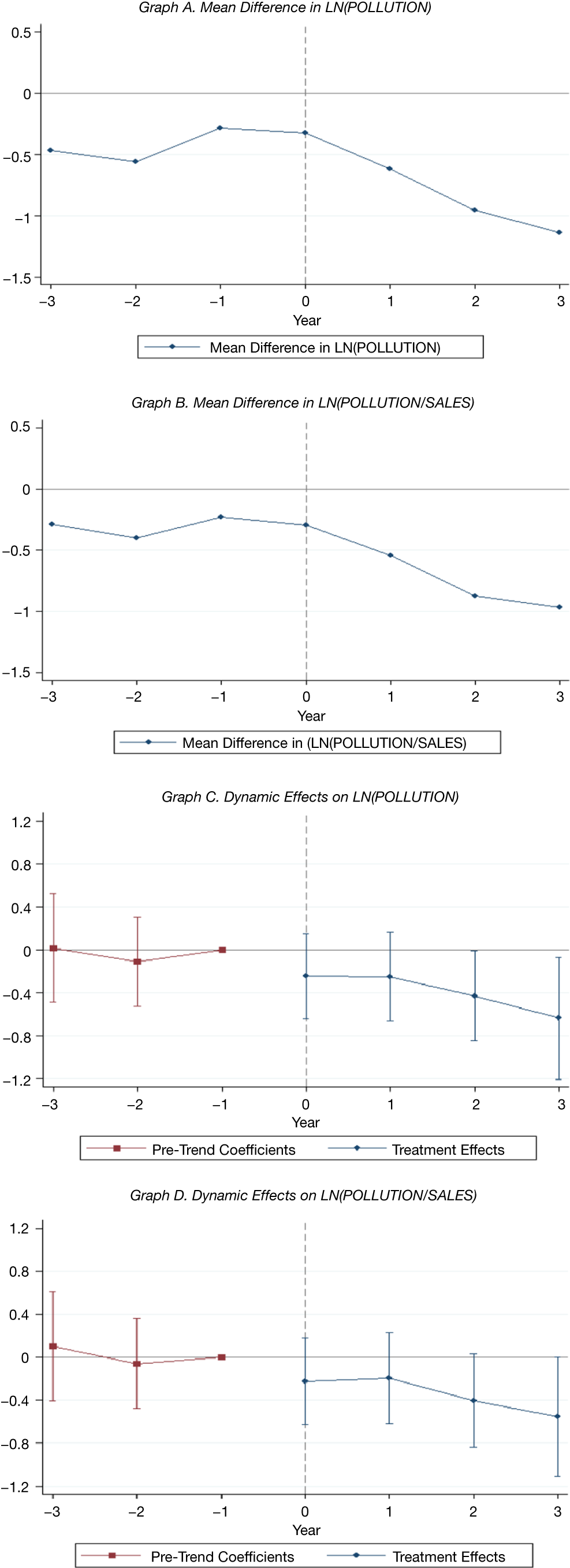
Graphs A and B of Figure 1 show that the mean difference in pollution between the treatment and control groups remains stable in the pre-treatment period (t – 3 to t – 1) and only begins to diverge in the post-treatment period, suggesting that the parallel trends assumption is not violated. Table 5 reports the DiD estimation results. Columns 1 and 4 present the results without controls, whereas columns 2 and 5 report the results from estimating equation (3) with controls. In all these columns, the coefficients on TREATED×AFTER are negative and statistically significant, suggesting that firms significantly reduce pollution in response to an exogenous increase in federal government procurement. In terms of economic magnitude, columns 2 and 5 indicate that treated firms reduce total pollution and sales-adjusted pollution by 29.7% (exp(−0.352) – 1) and 29.7% (exp(−0.353) – 1), respectively, relative to control firms. These results suggest that the plausibly exogenous increase in federal government procurement following congressional chairman turnovers is associated with a significant reduction in pollution by government contractors.
Graphs A and B of Figure 1 show the mean difference in i) the natural logarithm of the total pollution (LN(POLLUTION)) and ii) the natural logarithm of the total sales-adjusted pollution (LN(POLLUTION/SALES)), respectively, between treated and control firms from 3 years before (t – 3) to 3 years after (t + 3) the congressional chairman turnovers. Graphs C and D of Figure 1 show the coefficient estimates and 95% confidence intervals of the dynamic effects of congressional chairman turnovers on LN(POLLUTION) and LN(POLLUTION/SALES), respectively. See columns 3 and 6 of Table 5 for additional details.


To explore the timing of changes in pollution around chair turnovers, we estimate dynamic DiD models in columns 3 and 6. In these models, we replace AFTER in equation (3) with a set of indicators for the 2 pre-treatment years (BEFORE−3, BEFORE−2) and 4 post-treatment years (AFTER0, AFTER+1, AFTER+2, AFTER+3), using BEFORE−1 as the base year. The coefficients on TREATED×BEFORE−3 and TREATED×BEFORE−2 are statistically insignificant, indicating no pre-trend. Conversely, the coefficients on TREATED×AFTER+2 and TREATED×AFTER+3 are negative and statistically significant, suggesting that the treatment effect is reasonably persistent (see the plot of regression coefficients in Graphs C and D of Figure 1).
Overall, our DiD analysis supports the view that contractor firms reduce toxic pollution in response to government customer monitoring. However, we caution that our DiD analysis does not fully address endogeneity concerns; rather, it increases our confidence that the observed relation between government procurement and corporate pollution is not spurious. In the absence of perfect quasi-experiments, we adopt the “complementary approach” (Armstrong, Kepler, Samuels, and Taylor (Reference Armstrong, Kepler, Samuels and Taylor2022)), focusing on economic mechanisms, falsifying alternative explanations, and triangulating results across multiple settings and specifications, as described in Sections IV and V.
IV. Mechanisms
A. Internal Environmental Governance
Our results so far suggest that government scrutiny induces contractor firms to curb toxic pollution. However, it is still unclear how government customers influence the policies contractors may adopt to combat pollution. In this section, we explore two channels through which government customers affect contractors’ environmental performance. The first channel explores the possibility that firms with government customers are pressured to improve environmental performance by enhancing their internal environmental governance and providing training to employees. Specifically, we examine the effects of government customers on the likelihood of i) having a sustainability director and ii) providing environmental training.
First, we investigate whether government contractor firms are more likely to have a sustainability director. We obtain director information from the BoardEx database. Following Fu, Tang, and Chen (Reference Fu, Tang and Chen2020), a director is classified as a sustainability director if his or her job title contains any of the following words: sustainability, sustainable, responsibility, ethics, and environment. We then construct an indicator variable, SUSTAINABILITY DIRECTOR, that equals 1 for firm-years with at least one sustainability director, and 0 otherwise. The results in columns 1 and 2 of Panel A of Table 6 show a positive and statistically significant relationship between the government contracting variables and SUSTAINABILITY DIRECTOR, consistent with the notion that firms commit more internal governance resources to strengthen environmental responsibility in the presence of government customers.

Second, firms with government customers may enhance the environmental training of their employees to improve environmental performance. Using environmental training data from the Thomson Reuters ASSET4 database, and following Fiechter, Hitz, and Lehmann (Reference Fiechter, Hitz and Lehmann2022), we construct an indicator variable, ENV_TRAINING, that equals 1 if a company trains employees on environmental issues (e.g., resource reduction, emission reduction, and environmental-related codes of conduct), and 0 otherwise. The result in column 2 of Panel B of Table 6 shows a positive and significant relation between CONTRACT/SALES and ENV_TRAINING, supporting the view that firms with government customers improve environmental performance through training programs. Regarding economic significance, on average, a 1-unit increase in CONTRACT/SALES raises the likelihood of appointing a sustainability director and providing environmental management training by 1.26 and 3.35 percentage points, respectively.
B. Pollution Abatement Practices
In terms of the second channel, a contractor firm may increase investments in pollution abatement and prevention practices. This analysis exploits the fact that firms can reduce pollution by investing in pollution abatement activities, such as the development of green technologies and waste management systems (Akey and Appel (Reference Akey and Appel2021)). However, managers may lack the incentives to make such investments, especially when the probability of detecting corporate environmental misbehavior is low (Hart and Zingales (Reference Hart and Zingales2016)). Government customers’ monitoring makes it more difficult or costly to disguise environmentally irresponsible behavior. For this reason, we expect contractor firms under government scrutiny to be more likely to invest in pollution abatement and implement pollution prevention practices.
We first explore the effect of government customers on corporate investments in pollution abatement. Following Fiechter et al. (Reference Fiechter, Hitz and Lehmann2022), we collect information on corporate environmental investment initiatives from the Thomson Reuters ASSET4 database. Such initiatives involve investments in cleaner technologies that reduce the risk of future environmental issues and create opportunities for improvements in environmental practices and performance. We construct an indicator variable, ENV_INVESTMENT, that equals 1 if a firm makes environmental investments, and 0 otherwise. The result in column 2 of Panel A of Table 7 shows that firms with government customers are more likely to undertake investment initiatives in environmental protection and pollution abatement. A 1-unit increase in CONTRACT/SALES is associated with a 2.18 percentage point higher likelihood of making environmental investments.

Next, to analyze firms’ pollution abatement activities, we use the EPA’s Pollution Prevention (P2) database, which provides information on corporate practices that reduce, eliminate, or prevent pollution at its source before recycling, treatment, or disposal at the plant-chemical level (Akey and Appel (Reference Akey and Appel2019), (Reference Akey and Appel2021), Muthulingam, Dhanorkar, and Corbett (Reference Muthulingam, Dhanorkar and Corbett2022)).Footnote 14 The pollution abatement practices in the P2 database are broadly classified into operations-related and production-related pollution prevention practices. Operations-related practices aim to reduce toxic pollution and waste through improvements in operating processes and procedures, including good operating practices (e.g., improved maintenance scheduling and record-keeping), inventory control (e.g., efficient storage and management of chemicals and materials), and spill and leak prevention (e.g., monitoring programs and equipment inspections). Production-related practices, on the other hand, focus on improvements in techniques, materials, and equipment of the production process, including process modifications, surface preparation and finishing, cleaning and degreasing, product modifications, and raw material modifications.
In Panels B and C of Table 7, we examine the effect of government customers on contractors’ operations-related and production-related pollution abatement activities, respectively. Panel B reports the regression results for the overall operations-related pollution prevention practices. The results for the subcomponent practices (i.e., good operating practice, inventory control, and spill and leak prevention) are reported in Panel A of Supplementary Material Table A2. We find that government customers significantly increase suppliers’ operations-related pollution abatement activities, both in terms of the overall practices and the three subcomponent practices. According to column 2 of Panel B, a 1-unit increase in CONTRACT/SALES is associated with a 0.95 percentage point higher likelihood of investing in operations-related pollution prevention practices.
We then turn to production-related pollution abatement activities. Panel C of Table 7 reports the regression results for the overall production-related pollution prevention practices. The results for the subcomponent practices (i.e., process modifications, surface preparation and finishing, cleaning and degreasing, product modifications, and raw material modifications) are reported in Panel B of Supplementary Material Table A2. The results show that government customers significantly increase suppliers’ production-related pollution abatement activities, particularly those related to raw material and cleaning and degreasing. According to column 2 of Panel C, a 1-unit increase in CONTRACT/SALES is associated with a 0.78 percentage point higher likelihood of investing in production-related pollution prevention practices. Our evidence suggests that implementing a range of operations-related and production-related pollution abatement practices is an important channel through which government customers improve corporate environmental performance.
Moreover, in column 3 of each panel of Tables 6 and 7, we perform the corresponding DiD analyses based on congressional chairman turnovers and find largely consistent evidence. The turnovers are associated with increases of 10.6 percentage points in the likelihood of environmental management training, 11.67 percentage points in environmental investments, 6.67 percentage points in operations-related pollution prevention investments, and 7.95 percentage points in production-related pollution prevention investments among treated firms, relative to control firms. To sum up, the results from the mechanism analysis suggest that government customers can improve corporate environmental performance through two main channels: enhancing internal environmental governance and training, and increasing investments in pollution abatement and prevention practices.
V. Alternative Explanations and Additional Analysis
A. Reduction in Firm Economic Activities as an Alternative Explanation
This section examines an alternative explanation for the negative relationship between government customers and corporate pollution. The decline in a government contractor’s pollution could be due to a reduction in its economic activities. Indeed, Akey and Appel (Reference Akey and Appel2021) show that firms can reduce toxic pollution by downsizing their economic activities. To investigate this possibility, we examine whether having government customers significantly reduces a firm’s production activities and employment growth.
Our measure of firm production activities is the production ratio, which is commonly used in previous studies (e.g., Berrone and Gomez-Mejia (Reference Berrone and Gomez-Mejia2009), Akey and Appel (Reference Akey and Appel2019), (Reference Akey and Appel2021), Naaraayanan et al. (Reference Naaraayanan, Sachdeva and Sharma2021)). We collect production ratio data from the TRI database. Following Akey and Appel (Reference Akey and Appel2019), (Reference Akey and Appel2021), we exclude production ratios below 0 or above 5 to minimize data errors. The EPA requires facilities to report the ratio of their current-year production volume to the previous year’s production volume (Berrone and Gomez-Mejia (Reference Berrone and Gomez-Mejia2009)). To construct the firm-level production ratio variable (PRODUCTION RATIO), we aggregate the production ratios across all plants for each firm-year. The results in columns 1 and 2 of Panel A of Table 8 show that government customers do not have a significant impact on suppliers’ production activities.

We also explore a firm’s employment growth as a proxy for its economic activities (Akey and Appel (Reference Akey and Appel2021)). In columns 4 and 5 of Panel A of Table 8, we examine whether the presence of government customers reduces the supplier firm’s EMPLOYEE GROWTH, defined as the ratio of the current year’s number of employees to the previous year’s number of employees. Our results again show an insignificant effect of government customers on employment growth. In brief, we find no evidence that government contractors reduce pollution by lowering production or employment activities.
B. Relaxation of Financial Constraints as an Alternative Explanation
Another alternative explanation for our baseline results is that firms with government customers may have easier access to external financing (Dhaliwal et al. (Reference Dhaliwal, Judd, Serfling and Shaikh2016)). Such firms, facing fewer financial constraints, are more able to invest in pollution abatement, thereby improving corporate environmental performance (Xu and Kim (Reference Xu and Kim2022)). To test this conjecture, we explore whether having government customers reduces the financial constraints of contractor firms. We use two text-based measures of financial constraints developed by Hoberg and Maksimovic (Reference Hoberg and Maksimovic2015) and Bodnaruk et al. (Reference Bodnaruk, Loughran and McDonald2015). HM_FC captures the extent to which a firm is likely to delay future investments due to difficulties in accessing external financing (Hoberg and Maksimovic (Reference Hoberg and Maksimovic2015)). BLM_FC measures the frequency of financial constraints-related words in a firm’s 10-K filings (Bodnaruk et al. (Reference Bodnaruk, Loughran and McDonald2015)). For both measures, higher values indicate greater financial constraints.
In Panel B of Table 8, we regress these financial constraint measures on government contracting. The dependent variables are HM_FC in columns 1–3 and BLM_FC in columns 4–6. The results show that government customers do not have a significant impact on the financial constraints of supplier firms. These findings are confirmed by the DiD analyses based on congressional chairman turnovers in column 3 of Panels A and B. Our evidence suggests that government customers do not improve supplier environmental performance by reducing economic activities or alleviating financial constraints.
C. Ex Ante Selection Versus Ex Post Monitoring
Our main analysis suggests that the government plays an ex post monitoring role in procurement. However, corporate environmental performance may influence the ex ante selection of contractors in the first place (Flammer (Reference Flammer2018)). To examine this ex ante effect, we examine the impact of firm environmental violations (i.e., EPA enforcement cases) on government procurement. Panel A of Table 9 reports that environmental violations in the past 5 years (ENV_VIOLATIONS) significantly reduce the number of government contracts (LN(CONTRACT_N)) and the sales-scaled value of government contracts (CONTRACT/SALES). These findings are consistent with the argument that government customers consider the environmental track record of potential suppliers and exhibit reduced willingness to engage with those that have environmental violations.

Furthermore, to test the relative importance of ex ante selection and ex post monitoring effects, we conduct a DiD analysis using first-time government contract awards in our sample. Following Samuels (Reference Samuels2021), we identify first-time contractor firms that receive an initial contract award during our sample period as the treatment group. Since the treatments are staggered over time, we assemble our DiD sample in two steps. First, we match each treated firm to firms that are never treated, based on the same SIC 2-digit industry and size quartile in the year before becoming a government contractor. Using this matching procedure, we construct an event episode for each observation in the treatment group, consisting of the 3 years before (years t – 3 to t – 1) and 4 years after (years t to t + 3) the event. Second, we stack the data across all event episodes and estimate a standard DiD model as follows:
 $$ {POLLUTION}_{i,t+1}={\displaystyle \begin{array}{l}\alpha +{\beta}_1 FIRST\_{CONTRACT}_{i,t}\times {POST}_{i,t}\\ {}+\hskip2px {\beta}_2 FIRST\_{CONTRACT}_{i,t}+{\beta}_3{POST}_{i,t}+\delta {X}_{i,t}+{\lambda}_j\\ {}+\hskip2px {\mu}_t+{\varepsilon}_{i,t},\end{array}} $$
where FIRST_CONTRACT is a dummy variable that equals 1 if it is the first time a firm receives a government contract in year t, and 0 otherwise. POST is a dummy variable that takes the value of 1 for the 4 years after the treatment, and 0 otherwise. The main coefficients of interest are $ {\beta}_1 $
and
$ {\beta}_1 $
and $ {\beta}_2 $
that capture the ex post monitoring effect and the ex ante selection effect, respectively.
$ {\beta}_2 $
that capture the ex post monitoring effect and the ex ante selection effect, respectively. $ {\beta}_1 $
measures the effect of receiving a government contract for the first time on the firm’s environmental performance.
$ {\beta}_1 $
measures the effect of receiving a government contract for the first time on the firm’s environmental performance. $ {\beta}_2 $
measures the difference in firm environmental performance between the treatment and control groups in the pre-treatment period.
$ {\beta}_2 $
measures the difference in firm environmental performance between the treatment and control groups in the pre-treatment period.
Panel B of Table 9 presents our DiD estimation results. Columns 1 and 2 report the results from estimating equation (4). The coefficients on FIRST_CONTRACT×POST are negative and statistically significant at the 5% level or better, suggesting that first-time contractors significantly reduce toxic pollution after beginning to contract with the government, relative to otherwise similar control firms. The coefficients on FIRST_CONTRACT are also negative and statistically significant at the 10% level, indicating that government contractors perform better environmentally even before establishing business relationships with the government. In terms of economic magnitude, column 1 indicates that in the pre-treatment period, the total pollution of treated firms is 44% (exp(−0.58) – 1) lower, and that after the treatment, treated firms reduce total pollution further by 36.8% (exp(−0.459) – 1), relative to control firms.
Overall, our analyses of the effect of first-time contract awards not only lend further credence to the interpretation that contractor firms reduce toxic pollution in response to monitoring by government customers, but also provide evidence of an ex ante selection effect. Collectively, evidence on ex ante selection and ex post monitoring substantiates the idea that government customers increase the consequences of firms’ environmental misbehavior, thereby promoting better corporate environmental performance.
D. Other Environmental Governance Forces
Our baseline results may be affected by various environmental governance forces that are correlated with both the likelihood of winning government contracts and corporate environmental performance. To address this concern, we incorporate a range of additional environmental governance forces into our analysis. These forces include institutional ownership (Dyck, Lins, Roth, and Wagner (Reference Dyck, Lins, Roth and Wagner2019)), analyst coverage (Jing et al. (Reference Jing, Keasey, Lim and Xu2024)), regulatory enforcement (Seltzer, Starks, and Zhu (Reference Seltzer, Starks and Zhu2022)), local political ideology (Di Giuli and Kostovetsky (Reference Di Giuli and Kostovetsky2014)), and media coverage of firm environmental incidents (Duchin, Gao, and Xu (Reference Duchin, Gao and Xu2025)).
In Panel A of Table 10, we include several additional controls. IO is the natural logarithm of the percentage of shares held by institutional investors (times 100) plus 1. ANALYST is the natural logarithm of the average number of monthly earnings forecasts for a firm-year plus 1. ENFORCEMENT is a firm-level measure of regulatory stringency, calculated as the average state EPA enforcement intensity (i.e., the number of enforcement actions divided by the number of plants in the state) across a firm’s plants. BLUE is an indicator that equals 1 if a firm is headquartered in a county that predominantly voted for a Democratic presidential candidate in a recent election, and 0 otherwise. INCIDENTS is an indicator variable that equals 1 if a firm has at least one environmental risk event in the RepRisk database in a year, and 0 otherwise.Footnote 15

Our results are robust to controlling for these various sources of environmental pressures. Both the statistical and economic significance of government contracting variables remain comparable to the baseline results shown in Table 3. Among the additional control variables, only institutional ownership has a significantly negative impact on corporate pollution, consistent with the literature showing that institutional investors positively influence corporate environmental performance (Dyck et al. (Reference Dyck, Lins, Roth and Wagner2019)). In terms of economic magnitude, a 1% increase in the number of government contracts and institutional ownership corresponds to a 0.081% and 0.156% reduction in corporate pollution, respectively, suggesting that government contracting plays a crucial role in reducing corporate pollution.
E. Additional Robustness Tests
In Table 10, we perform a series of additional robustness tests. First, 1 might argue that our baseline finding is driven by a small number of firms with large government contracts. To test the sensitivity of our results to observations in different parts of the contract size distribution, we redefine LN(CONTRACT_N) and CONTRACT/SALES using different thresholds (i.e., 10,000, 1,000,000, and 100,000,000 USD). For instance, in row 1 of Panel B, a supplier firm is considered to have government contracts if the value of a contract exceeds 10,000 USD. The corresponding sales-scaled measure, CONTRACT/SALES, is likewise defined based on the 10,000 USD threshold. Overall, Panel B demonstrates that the effect of government customers on corporate pollution holds across the contract size distribution.
Second, we repeat baseline regressions using three alternative measures of government contracting. HAVE_CONTRACT is an indicator variable that equals 1 if a firm is awarded at least one government contract in a year, and 0 otherwise. LN(CONTRACT_VALUE) is the natural logarithm of the amount of federal award dollars in a year plus 1. CONTRACT/SALES (QUINTILE) is the quintile rank of CONTRACT/SALES (Samuels (Reference Samuels2021)). Panel C of Table 10 reports that our main finding is robust to these alternative measures of government contracting.
Third, to examine whether our results are specific to contracts from environmental regulators (i.e., the EPA) that are better able to monitor environmental issues than other government agencies, we reconstruct the government contracting variables after excluding contracts awarded by the EPA. Panel D of Table 10 reports that firms with non-EPA government contracts have significantly lower pollution, suggesting that non-EPA government agencies also contribute to disciplining supplier pollution practices.
Fourth, we use two alternative measures of corporate pollution. Following Clarkson, Li, and Richardson (Reference Clarkson, Li and Richardson2004) and Naaraayanan et al. (Reference Naaraayanan, Sachdeva and Sharma2021), we employ two output-adjusted measures of toxic emissions. LN(POLLUTION/AT) and LN(POLLUTION/COGS) are total pollution scaled by total assets and cost of goods sold, respectively. Panel E of Table 10 shows that the results remain consistent.
Fifth, a potential concern is that our results may be influenced by unobserved time-varying differences between firms with and without government contracts. This type of heterogeneity is not captured by firm fixed effects. To address this concern, we rerun our baseline regressions on a subsample of firms with at least one government contract award during the sample period. Panel F of Table 10 reports that our results continue to hold after excluding firms that have not received any government contracts throughout the entire sample period, indicating that our baseline results are driven by omitted time-varying characteristics of firms without government contracts.
To mitigate the concern that our results may be biased due to unobserved time-varying industry or state heterogeneity (e.g., industry or state regulatory changes), we control for additional fixed effects. Specifically, we include not only firm fixed effects but also industry-year and state-year interaction fixed effects. Panel G of Table 10 confirms that the results are robust to the inclusion of these additional fixed effects.
In addition, to further assess whether our results are driven by confounding factors, we conduct a placebo test by examining the environmental performance of pseudo-contractors. Pseudo-contractors are firms that, while not government contractors, offer products similar to those of government contractors. Since these firms have no direct customer-supplier relationship with the government, it is unlikely that government customers influence their pollution through monitoring. Therefore, we expect that being a pseudo-contractor should not affect a firm’s pollution.
In this placebo test, we replace GOV_CONTRACT in equation (1) with PSEUDO_CONTRACTOR, which equals 1 if a firm without government contracts (i.e., a non-contractor) is the closest competitor of a government contractor in a year, and 0 otherwise. For each government contractor in a year, we identify the non-contractor with the highest product similarity score relative to the contractor. Specifically, we use firm pairwise product similarity scores derived from the text analysis of firm product descriptions in 10-K filings to identify the closest competitors of government contractors (Hoberg and Phillips (Reference Hoberg and Phillips2016)). Panel H of Table 10 reports that the coefficient on PSEUDO_CONTRACTOR is statistically insignificant, reinforcing our confidence that the baseline results are attributable to government customer monitoring.
Next, to deal with the skewness of the pollution measure, we follow Dasgupta, Huynh, and Xia (Reference Dasgupta, Huynh and Xia2023) and use a standardized toxic pollution measure, STANDARDIZED_POLLUTION, as the dependent variable. This measure is defined as the ratio of the difference between a firm’s total toxic pollution and the industry average pollution to its standard deviation in each year. In columns 1 and 2 of Panel I of Table 10, we find that the results are robust to this standardized pollution measure.
Furthermore, our results are robust to an alternative estimation method that accounts for overdispersion (i.e., the conditional mean is greater than the conditional variance of the pollution measure). Given the overdispersion in our pollution data, we use the negative binomial estimator, which accommodates overdispersion by modeling variance as a separate gamma process. This method is used as an alternative to the Poisson estimator in cases of overdispersion (Cameron and Trivedi (Reference Cameron and Trivedi2005), Greene (Reference Greene2017), and Cohn, Liu, and Wardlaw (Reference Cohn, Liu and Wardlaw2022)).Footnote 16 Columns 3 and 4 of Panel I of Table 10 report that the results from negative binomial regressions align with our baseline results.
To gain a more comprehensive understanding of the environmental impact of government procurement, we extend our analysis to another important aspect of corporate environmental performance: carbon emissions. We examine the effect of government customers on corporate carbon emissions using two firm-level measures from the Trucost database for the period of 2005–2019. Following Bolton and Kacperczyk (Reference Bolton and Kacperczyk2021), (Reference Bolton and Kacperczyk2023), CARBON_GR is the growth rate of a firm’s direct emissions from production and indirect emissions from energy consumption in a year, and CARBON INTENSITY is the ratio of a firm’s total carbon emissions to total sales in a year. The former reflects a firm’s short-term tendency to adjust future emissions, whereas the latter has been a key focus for practitioners and investors (Bolton and Kacperczyk (Reference Bolton and Kacperczyk2023)). In Panel J of Table 10, we find that government customers significantly reduce both the growth and intensity of carbon emissions, indicating that the environmental impact of government procurement extends beyond reducing toxic pollution to lowering carbon emissions.
Finally, in Panel K of Table 10, we examine the timing of firm responses to government monitoring. We find that receiving government contracts in year t has a significantly negative effect on corporate pollution not only in year t + 1 (i.e., the baseline results), but also in years t + 2 and t + 3, suggesting that the effect of government procurement is reasonably persistent. Overall, our results remain robust across various alternative measures of government contracting and pollution, as well as different model specifications and estimation methods.
VI. Conclusions
This study explores the effect of government customers on corporate environmental policies. We find that firms with federal government contracts significantly reduce toxic emissions, consistent with the external governance role of government customers in improving supplier environmental performance. The finding is robust to a DiD analysis that mitigates endogeneity concerns. Further cross-sectional analyses show that the effect of government customers on corporate pollution is stronger in subsets of firms under greater government scrutiny, in firms whose revenue relies more on government contracts, and in firms that are not politically connected, consistent with a monitoring role of government customers in disciplining supplier pollution.
We document two channels through which government contractor firms improve environmental performance. First, contractor firms are more likely to establish internal environmental governance mechanisms, such as appointing a corporate sustainability director and providing environmental management training. Second, contractor firms significantly increase their investments in pollution abatement and prevention practices. Finally, we rule out alternative explanations pertaining to reduced economic activities and lower financial constraints. Overall, the results highlight the important external governance role of the government as a customer in shaping suppliers’ environmental policies.
Appendix: Variable Definitions
The following table presents the definitions and data sources of the main variables used in our empirical analysis.

Supplementary Material
To view supplementary material for this article, please visit http://doi.org/10.1017/S0022109025102111.


 Open access