


1. Introduction
Vortex dynamics, interaction and merging are fundamental aspects of fluid motion. The dynamics of two vortices has been of great interest and subject to much study both theoretically and experimentally; see Widnall (Reference Widnall1975) and Leweke, Dizes & Williamson (Reference Leweke, Dizes and Williamson2016) for reviews. The merging of three or more vortices has not been studied in similar detail although it is of great interest in order to understand more complex fluid motion emerging in nature or industry. One reason for the lack of study is the increasing complexity, well known in the celestial counterpart – the three body problem. As a step towards understanding the fluid motion of three vortices we here choose a special initial condition for the vortices, although several parameters still have arbitrary values. We investigate theoretically and computationally two-dimensional vortex merging starting with three aligned vortices, as shown in figure 1. In a point vortex setting (i.e. negligible viscosity), this initial configuration is a relative equilibrium, meaning that, depending on the vortex strengths, the vortices will stay fixed or rotate steadily but always maintain their mutual distances. However, in viscous flow, merging will always happen if the sum of the vortex strengths is non-zero since the long-term solution converges to the flow of a single Lamb–Oseen vortex, as proved by Gallay & Wayne (Reference Gallay and Wayne2005). We investigate the viscous merging of three aligned vortices for any centre vortex strength. A special case of this set-up has been investigated by Jing, Kanso & Newton (Reference Jing, Kanso and Newton2010) with the middle vortex rotating oppositely to the outer vortices and with half their strength. The vortex tripole experiment by van Heijst & Kloosterziel (Reference van Heijst and Kloosterziel1989) has also been modelled with three aligned vortices and corresponds to the case where the total vorticity vanishes. For small values of the centre vortex, the configuration is a perturbation to the well-studied case of two symmetric vortices (Cerretelli & Williamson Reference Cerretelli and Williamson2003; Meunier, Le Dizes & Leweke Reference Meunier, Le Dizes and Leweke2005). A benefit of the set-up chosen here will turn out to be the analytical insight from the core-growth model (described below), owing to the symmetry in the initial condition.
The flow is governed by the vorticity transport equation (VTE) in the unbounded plane
 \begin{align} \frac {\partial \omega }{\partial t}=-\boldsymbol{u}\boldsymbol{\cdot }\boldsymbol{\nabla }\omega + \nu \Delta \omega , \end{align}
where $\nu$
is the kinematic viscosity,
$\nu$
is the kinematic viscosity, $\boldsymbol{u}$
is the two-dimensional velocity field and
$\boldsymbol{u}$
is the two-dimensional velocity field and $\omega$
is the non-trivial component of the vorticity, defined as the curl of the velocity.
$\omega$
is the non-trivial component of the vorticity, defined as the curl of the velocity.
To characterise the flow patterns the vorticity contours are investigated. These are organised by the critical points of the vorticity, $\partial _x\omega (x,y)=\partial _y\omega (x,y)=0$
which come in two generic variants: local extremal points or saddle points which can be categorised from higher-order derivatives of the vorticity. Extremal points can be identified as vortices in the flow, while the saddle points have no physical interpretation, but must be identified to precisely describe the vortex patterns and their transitions. This approach has previously been used to investigate the occurrence of the von Kármán vortex street (Heil et al. Reference Heil, Rosso, Hazel and Brøns2017) and merging of two vortices (Brøns et al. Reference Brøns, Ozdemir, Heil, Andersen and Hansen2025). A similar topological investigation focusing on the streamfunction rather than the vorticity has been used extensively to study other flow configurations (Tobak & Peake Reference Tobak and Peake1982; Brøns Reference Brøns2007). The vorticity topology is Galilean invariant, but the streamline topology is not, so we focus on the former here.
$\partial _x\omega (x,y)=\partial _y\omega (x,y)=0$
which come in two generic variants: local extremal points or saddle points which can be categorised from higher-order derivatives of the vorticity. Extremal points can be identified as vortices in the flow, while the saddle points have no physical interpretation, but must be identified to precisely describe the vortex patterns and their transitions. This approach has previously been used to investigate the occurrence of the von Kármán vortex street (Heil et al. Reference Heil, Rosso, Hazel and Brøns2017) and merging of two vortices (Brøns et al. Reference Brøns, Ozdemir, Heil, Andersen and Hansen2025). A similar topological investigation focusing on the streamfunction rather than the vorticity has been used extensively to study other flow configurations (Tobak & Peake Reference Tobak and Peake1982; Brøns Reference Brøns2007). The vorticity topology is Galilean invariant, but the streamline topology is not, so we focus on the former here.
We investigate the vorticity contours based on the VTE, and compare the results with the core-growth model which allows for analytical investigation of viscous vortex interaction and merging (Jing, Kanso & Newton Reference Jing, Kanso and Newton2012; Kim & Sohn Reference Kim and Sohn2012). Conveniently expressed in complex form with $z=x+\text{i}y$
, the motion of a Gaussian vortex centre at
$z=x+\text{i}y$
, the motion of a Gaussian vortex centre at $z_j$
with strength
$z_j$
with strength $\varGamma_{\kern-1pt j}$
is governed by the position of the remaining
$\varGamma_{\kern-1pt j}$
is governed by the position of the remaining $N-1$
vortices
$N-1$
vortices
 \begin{align} {\frac {\text{d} \overline {z_j}}{\text{d} t}} = \sum _{k \neq j}^{N} \frac {\varGamma _k}{2 \pi \text{i}} \frac {1}{z_j - z_k} \left ( 1 - \exp {\left ( - \frac {{|z_j - z_k|}^2}{4\nu t} \right )} \right )\!, \end{align}
where $\overline {z}$
is the complex conjugate of
$\overline {z}$
is the complex conjugate of $z$
. The resulting velocity field is
$z$
. The resulting velocity field is
 \begin{align} {\frac {\text{d} \overline {z}}{\text{d} t}} = \sum _{k=1}^{N} \frac {\varGamma _k}{2 \pi \text{i}} \frac {1}{z - z_k} \left ( 1 - \exp {\left ( - \frac {{|z - z_k|}^2}{4\nu t} \right )} \right )\!. \end{align}
The corresponding vorticity being the curl of the velocity is
 \begin{align} \omega (z,t) = \sum _{k=1}^{N} \frac {\varGamma _k}{4 \pi \nu t} \exp {\left ( - \frac {{|z - z_k|}^2 }{4 \nu t} \right )}. \end{align}
In our study, $N=3$
and the initial condition is three point vortices on a straight line, see figure 1,
$N=3$
and the initial condition is three point vortices on a straight line, see figure 1,
 \begin{align} \omega (z,0)=\varGamma \delta (z-r_0)+\alpha \varGamma \delta (z)+\varGamma \delta (z+r_0). \end{align}
The strength of the outer vortices is $\varGamma$
and the strength of the centre vortex is
$\varGamma$
and the strength of the centre vortex is $\alpha \varGamma$
, where
$\alpha \varGamma$
, where $\alpha \in \mathbb{R}$
. The case
$\alpha \in \mathbb{R}$
. The case $\alpha =-2$
corresponds to the vortex tripole experiment (van Heijst & Kloosterziel Reference van Heijst and Kloosterziel1989) and the case
$\alpha =-2$
corresponds to the vortex tripole experiment (van Heijst & Kloosterziel Reference van Heijst and Kloosterziel1989) and the case $\alpha = -0.5$
corresponds to the point vortex equilibrium, studied by Jing et al. (Reference Jing, Kanso and Newton2010) with the purpose of elucidating the advection of passive tracers in a flow. For
$\alpha = -0.5$
corresponds to the point vortex equilibrium, studied by Jing et al. (Reference Jing, Kanso and Newton2010) with the purpose of elucidating the advection of passive tracers in a flow. For $\alpha =0$
we retrieve the well-studied case of two corotating vortices (Leweke et al. Reference Leweke, Dizes and Williamson2016; Andersen et al. Reference Andersen, Schreck, Hansen and Brøns2018). The velocity and vorticity given by the core-growth model, (1.2)–(1.4), is only an exact solution to VTE for
$\alpha =0$
we retrieve the well-studied case of two corotating vortices (Leweke et al. Reference Leweke, Dizes and Williamson2016; Andersen et al. Reference Andersen, Schreck, Hansen and Brøns2018). The velocity and vorticity given by the core-growth model, (1.2)–(1.4), is only an exact solution to VTE for $N=1$
. However, the core-growth model has shown to be useful to study vortex interaction for
$N=1$
. However, the core-growth model has shown to be useful to study vortex interaction for $N\gt 1$
(Kim & Sohn Reference Kim and Sohn2012; Nielsen et al. Reference Nielsen, Andersen, Hansen and Brøns2021; Dam, Hansen & Andersen Reference Dam, Hansen and Andersen2023). Kim & Sohn (Reference Kim and Sohn2012) show that the core-growth model with
$N\gt 1$
(Kim & Sohn Reference Kim and Sohn2012; Nielsen et al. Reference Nielsen, Andersen, Hansen and Brøns2021; Dam, Hansen & Andersen Reference Dam, Hansen and Andersen2023). Kim & Sohn (Reference Kim and Sohn2012) show that the core-growth model with $N$
vortices has integrals similar to the well-studied point vortex model, and prove that the well-known possibility of collapse of three point vortices (Synge Reference Synge1949; Aref Reference Aref1979) is not possible in the core-growth model. Nielsen et al. (Reference Nielsen, Andersen, Hansen and Brøns2021) use the core-growth model and the
$N$
vortices has integrals similar to the well-studied point vortex model, and prove that the well-known possibility of collapse of three point vortices (Synge Reference Synge1949; Aref Reference Aref1979) is not possible in the core-growth model. Nielsen et al. (Reference Nielsen, Andersen, Hansen and Brøns2021) use the core-growth model and the $Q$
-criterion to study merging of two vortices. Dam et al. (Reference Dam, Hansen and Andersen2023) obtain analytical insight into the merging of three vortices initially located at the corners of an equilateral triangle by use of the core-growth model.
$Q$
-criterion to study merging of two vortices. Dam et al. (Reference Dam, Hansen and Andersen2023) obtain analytical insight into the merging of three vortices initially located at the corners of an equilateral triangle by use of the core-growth model.
We aim to characterise vorticity contours of the core-growth model which requires the following approach: fix values for the parameters $\nu , \varGamma , \alpha , r_0$
and let the Gaussian vortex centres,
$\nu , \varGamma , \alpha , r_0$
and let the Gaussian vortex centres, $z_j$
, be governed by (1.2) with initial condition (1.5). Then, after solving for the Gaussian vortex centres, the vorticity is provided by (1.4). For any fixed
$z_j$
, be governed by (1.2) with initial condition (1.5). Then, after solving for the Gaussian vortex centres, the vorticity is provided by (1.4). For any fixed $t\gt 0$
we aim at locating and categorising the critical points of the vorticity. These critical points will in general change with time, so we need to consider time as a bifurcation parameter in this approach. Notice that we use the notation Gaussian vortex centres for
$t\gt 0$
we aim at locating and categorising the critical points of the vorticity. These critical points will in general change with time, so we need to consider time as a bifurcation parameter in this approach. Notice that we use the notation Gaussian vortex centres for $z_j$
, and extremal points of the vorticity for vortices. An important mathematical consequence of the symmetric initial condition turns out to be a closed-form expression for
$z_j$
, and extremal points of the vorticity for vortices. An important mathematical consequence of the symmetric initial condition turns out to be a closed-form expression for $z_j$
implying a closed-form expression of the vorticity in the core-growth model which simplifies the characterisation of the critical points of the vorticity.
$z_j$
implying a closed-form expression of the vorticity in the core-growth model which simplifies the characterisation of the critical points of the vorticity.

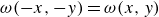
Figure 1. Initial conditions of the flow studied. Two equal point vortices are placed at $\pm (r_0,0)$
with a centre point vortex with arbitrary strength and direction.
$\pm (r_0,0)$
with a centre point vortex with arbitrary strength and direction.
2. Numerical method
The core-growth model is compared with results from numerical solutions to the VTE, (1.1). The method used follows Dam et al. (Reference Dam, Hansen and Andersen2023), which we here briefly summarise alongside some specific details. The VTE is solved together with the Poisson equation for the streamfunction $\Delta \psi = - \omega$
, giving the velocities
$\Delta \psi = - \omega$
, giving the velocities $\partial _x \psi = -u_2$
and
$\partial _x \psi = -u_2$
and $\partial _y \psi = u_1$
, where
$\partial _y \psi = u_1$
, where $u_1$
and
$u_1$
and $u_2$
are the velocity field vector components
$u_2$
are the velocity field vector components $\boldsymbol{u} = (u_1, u_2)$
. We use a fourth-order Runge–Kutta integrator for the solution to the VTE, see E & Liu (Reference E and Liu1996a
,Reference E and Liu
b
). The integrator time step is adaptive, and is implemented using extrapolation: at a given time
$\boldsymbol{u} = (u_1, u_2)$
. We use a fourth-order Runge–Kutta integrator for the solution to the VTE, see E & Liu (Reference E and Liu1996a
,Reference E and Liu
b
). The integrator time step is adaptive, and is implemented using extrapolation: at a given time $t$
with characteristic time step
$t$
with characteristic time step $h$
, the next integrated value at time
$h$
, the next integrated value at time $h+t$
of the vorticity is found from both a single-step integration, denoted
$h+t$
of the vorticity is found from both a single-step integration, denoted $\omega _h$
, and a two-step integration with time step
$\omega _h$
, and a two-step integration with time step $h/2$
, denoted
$h/2$
, denoted $\omega _{h/2}$
. If
$\omega _{h/2}$
. If $\text{max}| \omega _h - \omega _{h/2}|/\text{max}{|\omega _h|} \gt 0.01$
the time step is reduced by a factor 0.99 and it is otherwise increased by a factor 1.01. The spatial derivatives are approximated by the second-order central difference scheme, and the Poisson equation is solved using the spectral method, giving a significant speed up if the fast Fourier transform algorithm is applied.
$\text{max}| \omega _h - \omega _{h/2}|/\text{max}{|\omega _h|} \gt 0.01$
the time step is reduced by a factor 0.99 and it is otherwise increased by a factor 1.01. The spatial derivatives are approximated by the second-order central difference scheme, and the Poisson equation is solved using the spectral method, giving a significant speed up if the fast Fourier transform algorithm is applied.
The two-dimensional computational domain is set to $[-6;6] \times [-6;6]$
and discretised on a 512
$[-6;6] \times [-6;6]$
and discretised on a 512 $\times$
512 grid. Periodic boundary conditions are applied in both directions. The initial time step is set to
$\times$
512 grid. Periodic boundary conditions are applied in both directions. The initial time step is set to $h=1\times 10^{-6}$
. We use
$h=1\times 10^{-6}$
. We use $r_0=1$
and a vorticity strength of
$r_0=1$
and a vorticity strength of $\varGamma = 1$
. Because the Dirac delta initial condition induces numerical instabilities, we initialise the integration from a slightly diffused system corresponding to time
$\varGamma = 1$
. Because the Dirac delta initial condition induces numerical instabilities, we initialise the integration from a slightly diffused system corresponding to time $\Delta x^2/4\nu$
, where
$\Delta x^2/4\nu$
, where $\Delta x$
is the grid spacing. Moreover, since we apply periodic boundary conditions the vorticity is shifted such that the total vorticity is zero. The effect of the domain size and initial time step size were tested in the case
$\Delta x$
is the grid spacing. Moreover, since we apply periodic boundary conditions the vorticity is shifted such that the total vorticity is zero. The effect of the domain size and initial time step size were tested in the case $\alpha =1$
and
$\alpha =1$
and $1 \leqslant {Re} \leqslant 1000$
by letting the domain be
$1 \leqslant {Re} \leqslant 1000$
by letting the domain be $[-12;12] \times [-12;12]$
(corresponding to a 1024
$[-12;12] \times [-12;12]$
(corresponding to a 1024 $\times$
1024 grid) and
$\times$
1024 grid) and $h=2\times 10^{-6}$
. This showed no measurable difference on the computed merging time, which is found by tracking the vorticity extrema both visually and by numerical differentiation of the vorticity field. Finally, the Reynolds number is defined by
$h=2\times 10^{-6}$
. This showed no measurable difference on the computed merging time, which is found by tracking the vorticity extrema both visually and by numerical differentiation of the vorticity field. Finally, the Reynolds number is defined by ${Re}=\varGamma /\nu$
, that is, the Reynolds number is controlled directly by the viscosity in (1.1).
${Re}=\varGamma /\nu$
, that is, the Reynolds number is controlled directly by the viscosity in (1.1).
3. Analysis of the core-growth model and comparison with the VTE
We proceed analysing the core-growth model with the initial conditions seen in figure 1. We first show that $z_1(t),z_2(t)$
and
$z_1(t),z_2(t)$
and $z_3(t)$
stay aligned by a fixation of
$z_3(t)$
stay aligned by a fixation of $z_2$
and same angular velocities of
$z_2$
and same angular velocities of $z_1$
and
$z_1$
and $z_3$
.
$z_3$
.
The instantaneous velocity of the Gaussian vortex centres, $z_j$
, given by (1.2) is perpendicular to the line through them, initially the
$z_j$
, given by (1.2) is perpendicular to the line through them, initially the $x$
-axis as indicated in figure 1, suggesting that alignment of the Gaussian vortex centres is preserved. This is conveniently investigated by relying on the complex coordinate formulation. The ansatz of an aligned rotating configuration
$x$
-axis as indicated in figure 1, suggesting that alignment of the Gaussian vortex centres is preserved. This is conveniently investigated by relying on the complex coordinate formulation. The ansatz of an aligned rotating configuration
 \begin{align} z_k(t)=z_k(0)e^{{i}\phi (t)}\,,\quad k\in \left \{1,2,3\right \}\,,\quad \phi (0)=0\,, \end{align}
is inserted in (1.2) which is satisfied for
 \begin{align} \frac {{\rm d}\phi (t)}{{\rm d}t}=\frac {\varGamma }{2\pi r_0^2}\left (\alpha \left (1-e^{-\frac {r_0^2}{4\nu t}}\right )+\frac {1}{2}\left (1-e^{-\frac {r_0^2}{\nu t}}\right )\right )\!. \end{align}
As (3.2) is well defined for all $\nu t\gt 0$
, the ansatz is verified and the initially aligned Gaussian vortices stay aligned, by fixation of the centre Gaussian vortex, with the two outer vortices rotating with identical angular velocity. For
$\nu t\gt 0$
, the ansatz is verified and the initially aligned Gaussian vortices stay aligned, by fixation of the centre Gaussian vortex, with the two outer vortices rotating with identical angular velocity. For $\nu t \rightarrow 0$
the exponential terms vanish and the corresponding point vortex rotation rate is retrieved. For
$\nu t \rightarrow 0$
the exponential terms vanish and the corresponding point vortex rotation rate is retrieved. For $\nu t \rightarrow \infty$
,
$\nu t \rightarrow \infty$
, $ {{\rm d} \phi (t)}/{{\rm d}t}\rightarrow 0$
, i.e. the rotation rate vanishes due to viscosity.
$ {{\rm d} \phi (t)}/{{\rm d}t}\rightarrow 0$
, i.e. the rotation rate vanishes due to viscosity.
Numerical computation of the rotation angle can be accomplished to machine precision using the exponential integral $Ei(x)=\int _{x}^\infty t^{-1}e^{-t}{\rm d}t$
. To utilise this, (3.2) is integrated, relying on integration by parts and substitution to get
$Ei(x)=\int _{x}^\infty t^{-1}e^{-t}{\rm d}t$
. To utilise this, (3.2) is integrated, relying on integration by parts and substitution to get
 \begin{align} \phi (t)=\frac {\varGamma }{2\pi r_0^2}\left (\alpha \left (t-te^{-\frac {r_0^2}{4\nu t}}+\frac {r_0^2}{4\nu }Ei\left (\frac {r_0^2}{4\nu t}\right )\right )+\frac {1}{2}\left (t-te^{-\frac {r_0^2}{\nu t}}+\frac {r_0^2}{\nu }Ei\left (\frac {r_0^2}{\nu t}\right )\right )\right )\!. \end{align}
The positions of the Gaussian vortices are thus parametrised from (3.1) and (3.3).
For any fixed $t\gt 0$
we aim at describing the vorticity topology. This analysis is simplified by using a coordinate system with the
$t\gt 0$
we aim at describing the vorticity topology. This analysis is simplified by using a coordinate system with the $x$
-axis along the Gaussian vortex centres, which is accomplished by a rotation of the original coordinate system by the angle
$x$
-axis along the Gaussian vortex centres, which is accomplished by a rotation of the original coordinate system by the angle $\phi (t)$
. We define the viscous time,
$\phi (t)$
. We define the viscous time, $\tau$
, position, vorticity,
$\tau$
, position, vorticity, $\tilde {\omega }$
, and
$\tilde {\omega }$
, and $\tilde {z}$
 \begin{align} \tau = \frac {4 \nu }{r_0^2} t\,, \quad \tilde {\omega } = \frac {\pi r_0^2}{\varGamma } \omega \,, \quad \tilde {z} = \frac {1}{r_0} z. \end{align}
Relabelling (dropping the tilde $\tilde{\,}$
) the variables, the vorticity equation (1.4) appears as
$\tilde{\,}$
) the variables, the vorticity equation (1.4) appears as
 \begin{align} \omega =\frac {1}{\tau }\left (\exp {\left (-\frac {{|{z} + 1|}^2 }{\tau } \right )}+\alpha \exp {\left (-\frac {{|z|}^2 }{\tau } \right )}+\exp {\left (-\frac {{|{z} - 1|}^2 }{\tau } \right )}\right )\!. \end{align}
The Gaussian vortex centres, $z_j$
, are fixed at
$z_j$
, are fixed at $(0,0)$
and
$(0,0)$
and $(\pm 1,0)$
in the corotated system with the units introduced in (3.4). The task of investigating the vorticity topology is greatly simplified as the vorticity is explicitly parametrised depending on only two parameters,
$(\pm 1,0)$
in the corotated system with the units introduced in (3.4). The task of investigating the vorticity topology is greatly simplified as the vorticity is explicitly parametrised depending on only two parameters, $\alpha$
and
$\alpha$
and $\tau$
. Increasing
$\tau$
. Increasing $\nu$
corresponds to increasing
$\nu$
corresponds to increasing $\tau$
i.e. by changing
$\tau$
i.e. by changing $\nu$
the same vorticity patterns will be observed, however, the transition timing changes. The parameter
$\nu$
the same vorticity patterns will be observed, however, the transition timing changes. The parameter $\varGamma$
does not affect the vorticity patterns – it acts as a scaling on the vorticity. Increasing
$\varGamma$
does not affect the vorticity patterns – it acts as a scaling on the vorticity. Increasing $\varGamma$
gives a linear scaling of the rotation rate given by (3.2) which in scaled variables becomes
$\varGamma$
gives a linear scaling of the rotation rate given by (3.2) which in scaled variables becomes
 \begin{align} \frac {{\rm d} \phi }{{\rm d} \tau }=\frac {\varGamma }{\nu }\frac {1}{8\pi }\left (\alpha \left (1-e^{-\frac {1}{\tau }}\right )+\frac {1}{2}\left (1-e^{-\frac {4}{\tau }}\right )\right )\!. \end{align}
To facilitate the further calculations we proceed using Cartesian coordinates where (3.5) is given by
 \begin{align} \omega (x,y) =\frac {1}{\tau } \! \left ( \!\exp \! {\left (\!-\frac {\left (x+1\right )^2+y^2 }{\tau } \right )}+\alpha \exp {\!\left (-\frac {x^2+y^2 }{\tau } \right )}+\exp {\!\left (-\frac {\left (x-1\right )^2+y^2}{\tau } \right )}\!\right ). \end{align}
The vorticity field has reflection symmetry around the $x$
and
$x$
and $y$
axes, i.e.
$y$
axes, i.e. $\omega (-x,y)=\omega (x,y)=\omega (x,-y)$
, and symmetry by rotation of
$\omega (-x,y)=\omega (x,y)=\omega (x,-y)$
, and symmetry by rotation of $\pi$
, i.e.
$\pi$
, i.e. $\omega (-x,-y)=\omega (x,y)$
. The task is now to locate and characterise the critical points satisfying
$\omega (-x,-y)=\omega (x,y)$
. The task is now to locate and characterise the critical points satisfying $\partial _x \omega (x,y)=\partial _y \omega (x,y)=0$
 \begin{align}\partial _x \omega =&-\frac {2}{\tau ^2}\exp \! \left (\! -\frac {x^2+y^2}{\tau }\right )\left (\! \left (x+1\right )\exp \! \left ( \! -\frac {2x+1}{\tau }\right )+\alpha x+\left (x-1\right )\exp \! \left (\!\frac {2x-1}{\tau }\right )\!\right ) , \\[-12pt] \nonumber\end{align}
 \begin{align}\partial _y \omega =&-\frac {2y}{\tau }\omega, \end{align}
showing $(x,y)=(0,0)$
is a critical point of the vorticity for any
$(x,y)=(0,0)$
is a critical point of the vorticity for any $\tau \gt 0$
, and any
$\tau \gt 0$
, and any $\alpha$
value. The higher-order derivatives needed to characterise the critical points are
$\alpha$
value. The higher-order derivatives needed to characterise the critical points are
 \begin{align}\partial _{xx}\omega =& -\frac {2x}{\tau }\partial _x \omega -\frac {2}{\tau ^3}\exp \left (-\frac {x^2+y^2+1}{\tau }\right )\left (\left (\tau -2x-2\right )\exp \left (-\frac {2x}{\tau }\right )\right .\nonumber \\ &\left .+\alpha \tau \exp \left (\frac {1}{\tau }\right )+\left (\tau +2x-2\right )\exp \left (\frac {2x}{\tau }\right )\right )\!, \\[-12pt] \nonumber\end{align}
 \begin{align}\partial _{yy} \omega =&-\frac {2}{\tau }\omega -\frac {2y}{\tau }\partial _y\omega , \\[-12pt] \nonumber\end{align}
 \begin{align}\partial _{xy} \omega =&-\frac {2y}{\tau }\partial _x\omega .\end{align}
At a critical point, $\partial _x\omega =\partial _y\omega =0$
, in particular
$\partial _x\omega =\partial _y\omega =0$
, in particular $\partial _{xy}\omega =0$
at any critical point.
$\partial _{xy}\omega =0$
at any critical point.
3.1. Three corotating vortices
To proceed we distinguish between the cases $\alpha \gt 0$
and
$\alpha \gt 0$
and $\alpha \lt 0$
, two symmetric vortices (
$\alpha \lt 0$
, two symmetric vortices ( $\alpha =0$
) having been studied elsewhere (Andersen et al. Reference Andersen, Schreck, Hansen and Brøns2018). In this section we assume three corotating Gaussian vortices,
$\alpha =0$
) having been studied elsewhere (Andersen et al. Reference Andersen, Schreck, Hansen and Brøns2018). In this section we assume three corotating Gaussian vortices, $\alpha \gt 0$
, which implies that the rotation rate (3.2), of the collinear Gaussian vortices is always positive i.e. the three Gaussian vortices rotate counter-clockwise at all times. The vorticity field, (3.7), is a sum of positive terms and therefore
$\alpha \gt 0$
, which implies that the rotation rate (3.2), of the collinear Gaussian vortices is always positive i.e. the three Gaussian vortices rotate counter-clockwise at all times. The vorticity field, (3.7), is a sum of positive terms and therefore $y=0$
is needed for
$y=0$
is needed for $\partial _y \omega =0$
by (3.9). To characterise a critical point, we have from (3.11),
$\partial _y \omega =0$
by (3.9). To characterise a critical point, we have from (3.11), $\partial _{yy}\omega (x,0)\lt 0$
and from (3.12),
$\partial _{yy}\omega (x,0)\lt 0$
and from (3.12), $\partial _{xy}\omega (x,0)=0$
. Hence, if
$\partial _{xy}\omega (x,0)=0$
. Hence, if $\partial _{xx}\omega (x,0)\lt 0$
at the critical point, then it is an extremum of the vorticity field i.e. a vortex. If
$\partial _{xx}\omega (x,0)\lt 0$
at the critical point, then it is an extremum of the vorticity field i.e. a vortex. If $\partial _{xx}\omega (x,0)\gt 0$
at the critical point, then it is a saddle. For
$\partial _{xx}\omega (x,0)\gt 0$
at the critical point, then it is a saddle. For $x\geqslant 1$
, then
$x\geqslant 1$
, then $x+1, \alpha x$
are positive and
$x+1, \alpha x$
are positive and $x-1$
is non-negative, so
$x-1$
is non-negative, so $\partial _{x}\omega \lt 0$
in this case i.e. there are no critical points for
$\partial _{x}\omega \lt 0$
in this case i.e. there are no critical points for $x\geqslant 1$
. The task of locating critical points of the vorticity is then reduced to finding zeros of
$x\geqslant 1$
. The task of locating critical points of the vorticity is then reduced to finding zeros of $\partial _{x}\omega (x,0)$
for
$\partial _{x}\omega (x,0)$
for $0\lt x\lt 1$
for positive
$0\lt x\lt 1$
for positive $\tau ,\alpha$
, where we may use that
$\tau ,\alpha$
, where we may use that $\partial _{x}\omega$
is an odd function of
$\partial _{x}\omega$
is an odd function of $x$
. Trivially,
$x$
. Trivially, $(0,0)$
is a critical point. For
$(0,0)$
is a critical point. For $\partial _{xx}\omega \neq 0$
at any critical point, the intersections of
$\partial _{xx}\omega \neq 0$
at any critical point, the intersections of $\partial _{x}\omega (x,0)$
with the
$\partial _{x}\omega (x,0)$
with the $x$
axis occur with non-zero slope of
$x$
axis occur with non-zero slope of $\partial _x\omega$
. Since
$\partial _x\omega$
. Since $\partial _{x}\omega \lt 0$
for
$\partial _{x}\omega \lt 0$
for $x\geq 1$
, the critical point with the largest
$x\geq 1$
, the critical point with the largest $x$
value has
$x$
value has $\partial _{xx}\omega \lt 0$
and the sign of
$\partial _{xx}\omega \lt 0$
and the sign of $\partial _{xx}\omega$
is alternating for decreasing
$\partial _{xx}\omega$
is alternating for decreasing $x$
value. This implies that the outermost critical point of vorticity is a vortex, the next is a saddle, and so on with alternating type. The sign of
$x$
value. This implies that the outermost critical point of vorticity is a vortex, the next is a saddle, and so on with alternating type. The sign of $\partial _{xx}\omega (0,0)$
carries important information; if it is positive,
$\partial _{xx}\omega (0,0)$
carries important information; if it is positive, $(0,0)$
is a saddle point of the vorticity and there are at least two more critical points which must be vorticity extrema
$(0,0)$
is a saddle point of the vorticity and there are at least two more critical points which must be vorticity extrema
 \begin{align} \partial _{xx}\omega (0,0)=\frac {2}{\tau ^2}\exp \left (\frac {1}{\tau }\right )\left (2\frac {2-\tau }{\tau }\exp \left (-\frac {1}{\tau }\right )-\alpha \right )\!, \end{align}
which for $\alpha \gt 0$
is negative for
$\alpha \gt 0$
is negative for $\tau$
going to 0 or
$\tau$
going to 0 or $\tau \gt 2$
. Notice
$\tau \gt 2$
. Notice $2( {2-\tau })/{\tau }\exp (- {1}/{\tau })$
is increasing for
$2( {2-\tau })/{\tau }\exp (- {1}/{\tau })$
is increasing for $\tau \lt 2/3$
and decreasing for
$\tau \lt 2/3$
and decreasing for $\tau \gt {2}/{3}$
and has maximum value
$\tau \gt {2}/{3}$
and has maximum value
 \begin{align} \alpha _c=4\exp \left (-\frac {3}{2}\right ) \!. \end{align}
For $\tau _c=2/3$
there are three scenarios, see figure 2:
$\tau _c=2/3$
there are three scenarios, see figure 2: $0\lt \alpha \lt \alpha _c$
,
$0\lt \alpha \lt \alpha _c$
, $\alpha =\alpha _c$
and
$\alpha =\alpha _c$
and $\alpha \gt \alpha _c$
. For
$\alpha \gt \alpha _c$
. For $\alpha \lt \alpha _c$
,
$\alpha \lt \alpha _c$
, $\partial _{xx}\omega (0,0)\lt 0$
for small
$\partial _{xx}\omega (0,0)\lt 0$
for small $\tau$
, increasing
$\tau$
, increasing $\tau$
from a small value,
$\tau$
from a small value, $\partial _{xx}\omega (0,0)$
changes sign for some
$\partial _{xx}\omega (0,0)$
changes sign for some $\tau \lt 2/3$
i.e. transforms from a vortex to a saddle, and for some
$\tau \lt 2/3$
i.e. transforms from a vortex to a saddle, and for some $\tau \gt {2}/{3}$
,
$\tau \gt {2}/{3}$
, $\partial _{xx}\omega (0,0)$
changes sign and
$\partial _{xx}\omega (0,0)$
changes sign and $(0,0)$
remains a vortex for all larger
$(0,0)$
remains a vortex for all larger $\tau$
values. For
$\tau$
values. For $\alpha \gt \alpha _c$
,
$\alpha \gt \alpha _c$
, $(0,0)$
is a vortex for all positive
$(0,0)$
is a vortex for all positive $\tau$
. For the threshold case
$\tau$
. For the threshold case $\alpha =\alpha _c$
,
$\alpha =\alpha _c$
, $(0,0)$
is a vortex except for
$(0,0)$
is a vortex except for $\tau ={2}/{3}$
. A change in vorticity patterns occurs at a bifurcation point characterised by
$\tau ={2}/{3}$
. A change in vorticity patterns occurs at a bifurcation point characterised by $\partial _{x}\omega (x,y)=\partial _{xx}\omega (x,y)=0$
. This implies from (3.13) that, in the parameter space
$\partial _{x}\omega (x,y)=\partial _{xx}\omega (x,y)=0$
. This implies from (3.13) that, in the parameter space $(\tau ,\alpha )$
, the curve
$(\tau ,\alpha )$
, the curve
 \begin{align} \alpha =\left (\frac {4}{\tau }-2\right )\exp \left (-\frac {1}{\tau }\right ) \end{align}
is a bifurcation curve (blue curve figure 2
a). It is immediately clear that $\tau =2$
is a solution to (3.15) for
$\tau =2$
is a solution to (3.15) for $\alpha =0$
, which was previously reported by Andersen et al. (Reference Andersen, Schreck, Hansen and Brøns2018) for the merging of two vortices.
$\alpha =0$
, which was previously reported by Andersen et al. (Reference Andersen, Schreck, Hansen and Brøns2018) for the merging of two vortices.

Figure 2. (a) Bifurcation diagram for the core-growth model. The four regions have distinct vorticity patterns. (b) Illustrations of the four vorticity patterns in the core-growth model.
The location of other bifurcation values can be computed from $\partial _{x}\omega (x,0)=\partial _{xx}\omega (x,0)$
, which provides two equations for the three unknowns
$\partial _{x}\omega (x,0)=\partial _{xx}\omega (x,0)$
, which provides two equations for the three unknowns $\tau , \alpha , x$
. From
$\tau , \alpha , x$
. From $\partial _{x}\omega (x,0)=0$
,
$\partial _{x}\omega (x,0)=0$
, $\alpha$
can be solved for
$\alpha$
can be solved for
 \begin{align} \alpha =-\frac {x+1}{x}\exp \left (-\frac {2x+1}{\tau }\right )+\frac {1-x}{x}\exp \left (\frac {2x-1}{\tau }\right ). \end{align}
Inserting this expression into $\partial _{xx}\omega (x,0)=0$
gives one equation in the two unknowns
$\partial _{xx}\omega (x,0)=0$
gives one equation in the two unknowns $x$
and
$x$
and $\tau$
. With the definition
$\tau$
. With the definition $s= 2x/\tau$
this equation can be solved for
$s= 2x/\tau$
this equation can be solved for $x=f(s)$
with
$x=f(s)$
with
 \begin{align} f(s)=\coth (s)-\frac {1}{s}. \end{align}
The procedure for locating bifurcation points is then: pick any $s\gt 0$
, compute
$s\gt 0$
, compute $x=f(s)$
,
$x=f(s)$
, $\tau =2x/s$
and
$\tau =2x/s$
and $\alpha$
from (3.16) provides a parametrisation of all bifurcation points, in particular adding the black curve in figure 2(a). This analysis results in a complete description of all emerging flow patterns and their transitions for
$\alpha$
from (3.16) provides a parametrisation of all bifurcation points, in particular adding the black curve in figure 2(a). This analysis results in a complete description of all emerging flow patterns and their transitions for $\alpha \gt 0$
; see figures 2 and 3. For
$\alpha \gt 0$
; see figures 2 and 3. For $\alpha \gt \alpha _c$
, the initial vorticity field consisting of three aligned vortex maxima with a saddle between any two extrema (pattern (A)) merges to a single maxima and no saddles (pattern (C)) by two simultaneous saddle node bifurcations, where an outer vortex maximum and the nearest saddle merge and vanish (crossing the black curve in figure 2
a), i.e. the centre vortex dominates. For
$\alpha \gt \alpha _c$
, the initial vorticity field consisting of three aligned vortex maxima with a saddle between any two extrema (pattern (A)) merges to a single maxima and no saddles (pattern (C)) by two simultaneous saddle node bifurcations, where an outer vortex maximum and the nearest saddle merge and vanish (crossing the black curve in figure 2
a), i.e. the centre vortex dominates. For $\alpha _c\gt \alpha \gt 0$
pattern (A) change to pattern (B) with increasing time as the middle vorticity extrema merge with the two neighbouring saddles through a pitchfork bifurcation (crossing the full blue curve in figure 2
a) leaving a saddle at the origin, i.e. the centre vortex is suppressed. Then, pattern (B) changes to pattern (C) as an additional pitchfork bifurcation happens where the two outer vorticity maxima merge with the saddle (crossing the stipulated blue curve in figure 2
a) and leave a single vorticity maxima at the origin (pattern (C)).
$\alpha _c\gt \alpha \gt 0$
pattern (A) change to pattern (B) with increasing time as the middle vorticity extrema merge with the two neighbouring saddles through a pitchfork bifurcation (crossing the full blue curve in figure 2
a) leaving a saddle at the origin, i.e. the centre vortex is suppressed. Then, pattern (B) changes to pattern (C) as an additional pitchfork bifurcation happens where the two outer vorticity maxima merge with the saddle (crossing the stipulated blue curve in figure 2
a) and leave a single vorticity maxima at the origin (pattern (C)).
Trajectories of the critical points of vorticity can be obtained by numerically solving $\partial _x\omega (x,0)=0$
for fixed
$\partial _x\omega (x,0)=0$
for fixed $\alpha$
. This is illustrated in the top row of figure 3 which compares very well with solutions of the VTE for
$\alpha$
. This is illustrated in the top row of figure 3 which compares very well with solutions of the VTE for $Re=1$
.
$Re=1$
.

Figure 3. Position of critical points of the vorticity in the core-growth model (punctured curves) and for the VTE (dots) for $ {\varGamma }/{\nu }=1$
at different centre vortex strengths,
$ {\varGamma }/{\nu }=1$
at different centre vortex strengths, $\alpha$
. Vorticity maxima (blue), vorticity minima (red) and vorticity saddles (green) are shown. Panel (a) for
$\alpha$
. Vorticity maxima (blue), vorticity minima (red) and vorticity saddles (green) are shown. Panel (a) for $\alpha = 1.0$
, the vorticity pattern (A) persists until the outer vortices merge with the saddle points at
$\alpha = 1.0$
, the vorticity pattern (A) persists until the outer vortices merge with the saddle points at $\tau =0.48$
, leading to vorticity pattern (C), i.e. the centre vortex dominates. Panel (b) for the threshold value
$\tau =0.48$
, leading to vorticity pattern (C), i.e. the centre vortex dominates. Panel (b) for the threshold value $\alpha = \alpha _c$
, vorticity pattern (A) persists until
$\alpha = \alpha _c$
, vorticity pattern (A) persists until $\tau = {2}/{3}$
where all critical points of vorticity collide in a double pitchfork bifurcation leaving a single vorticity maximum, pattern (C). Panel (c) for
$\tau = {2}/{3}$
where all critical points of vorticity collide in a double pitchfork bifurcation leaving a single vorticity maximum, pattern (C). Panel (c) for $\alpha = 0.5$
, vorticity pattern (A) persists until
$\alpha = 0.5$
, vorticity pattern (A) persists until $\tau =0.35$
, where a pitchfork bifurcation happens leading to vorticity pattern (B), i.e. centre vortex suppression, until a pitchfork bifurcation happens at
$\tau =0.35$
, where a pitchfork bifurcation happens leading to vorticity pattern (B), i.e. centre vortex suppression, until a pitchfork bifurcation happens at $\tau =1.3$
where vorticity pattern (C) persists after merging of the two outer vortices. Panel (d) for the threshold value
$\tau =1.3$
where vorticity pattern (C) persists after merging of the two outer vortices. Panel (d) for the threshold value $\alpha = 0$
(no centre Gaussian vortex), vorticity pattern (B) exists until merging at
$\alpha = 0$
(no centre Gaussian vortex), vorticity pattern (B) exists until merging at $\tau = 2$
where a pitchfork bifurcation leads to vorticity pattern (C), as previously described by Andersen et al. (Reference Andersen, Schreck, Hansen and Brøns2018). Panel (e) for
$\tau = 2$
where a pitchfork bifurcation leads to vorticity pattern (C), as previously described by Andersen et al. (Reference Andersen, Schreck, Hansen and Brøns2018). Panel (e) for $\alpha = -0.5$
the initial vorticity pattern is type (D), then turning into type (B) through an instant of a line of critical points of the vorticity (see (3.23)), i.e. the centre vortex is suppressed. Then vorticity pattern (B) turns into (C) by a pitchfork bifurcation, where the two outer extrema of vorticity collapse with the saddle of vorticity leaving a single vorticity extrema. Panel (f) for
$\alpha = -0.5$
the initial vorticity pattern is type (D), then turning into type (B) through an instant of a line of critical points of the vorticity (see (3.23)), i.e. the centre vortex is suppressed. Then vorticity pattern (B) turns into (C) by a pitchfork bifurcation, where the two outer extrema of vorticity collapse with the saddle of vorticity leaving a single vorticity extrema. Panel (f) for $\alpha = -2.5$
, the vorticity pattern (D) persists as the outer vortices are moving outwards, i.e. the centre vortex dominates.
$\alpha = -2.5$
, the vorticity pattern (D) persists as the outer vortices are moving outwards, i.e. the centre vortex dominates.
The intersection of the bifurcation curves that appears to be located at $(\tau _c,\alpha _c)$
merits special attention. At this parameter set,
$(\tau _c,\alpha _c)$
merits special attention. At this parameter set, $(x,y)=(0,0)$
is a bifurcation point, which means a local investigation may be useful. We search for analytical expressions for critical points of the vorticity close to the origin by making a Taylor expansion of
$(x,y)=(0,0)$
is a bifurcation point, which means a local investigation may be useful. We search for analytical expressions for critical points of the vorticity close to the origin by making a Taylor expansion of $(x+1 )\exp (-({2x+1})/{\tau } )+\alpha x+ (x-1 )\exp (({2x-1})/{\tau } )$
, see (3.8), to sixth order in
$(x+1 )\exp (-({2x+1})/{\tau } )+\alpha x+ (x-1 )\exp (({2x-1})/{\tau } )$
, see (3.8), to sixth order in $x$
with coefficients depending on
$x$
with coefficients depending on $\tau$
and
$\tau$
and $\alpha$
. To accommodate for five critical points at least a fifth-order polynomial approximation,
$\alpha$
. To accommodate for five critical points at least a fifth-order polynomial approximation, $p(x)$
, of the vorticity is needed, which is given by
$p(x)$
, of the vorticity is needed, which is given by
 \begin{align} p(x)=x\big (\beta _1+\beta _2x^2+\beta _3x^4\big ) , \end{align}
with coefficients
 \begin{align} \beta _1&=\alpha -2\frac {2-\tau }{\tau }\exp {\left (-\frac {1}{\tau }\right )}, \\[-12pt] \nonumber \end{align}
 \begin{align} \beta _2&=\frac {4}{\tau ^3}\exp {\left (-\frac {1}{\tau }\right )}\left (\tau -\frac {2}{3}\right )\!, \\[-12pt] \nonumber \end{align}
 \begin{align} \beta _3&=\frac {4}{3\tau ^5}\exp {\left (-\frac {1}{\tau }\right )}\left (\tau -\frac {2}{5}\right )\!. \\[9pt] \nonumber \end{align}
The roots of the fifth-order polynomial, (3.18), can be analytically solved as only odd terms appear, one root is 0 and the remaining roots can be computed from the quadratic formula, solving for $x^2$
. Notice that
$x^2$
. Notice that $\beta _1=0$
corresponds to the bifurcation curve (3.15). The roots of (3.18) are
$\beta _1=0$
corresponds to the bifurcation curve (3.15). The roots of (3.18) are $x=0$
and up to four more solutions
$x=0$
and up to four more solutions
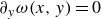
 \begin{align} x=\pm \sqrt {\frac {-\beta _2\pm \sqrt {D}}{2\beta _3}} , \end{align}
with $D=\beta _2^2-4\beta _1\beta _3$
. The curves in parameter space separating regions with one, three and five solutions are given by
$D=\beta _2^2-4\beta _1\beta _3$
. The curves in parameter space separating regions with one, three and five solutions are given by $\beta _1=0$
(figure 2 blue curve) and
$\beta _1=0$
(figure 2 blue curve) and $D=0$
(figure 2 black curve).
$D=0$
(figure 2 black curve).
The root calculation of (3.18) is summarised as:
-
(i) for $\alpha \lt 2( {2-\tau })/{\tau }\exp { (- {1}/{\tau } )}$
there are exactly three roots:
$x=0$
,
$x=\pm \sqrt{(-\beta_2+\sqrt{D})/(2\beta_3)}$
;
$\alpha \lt 2( {2-\tau })/{\tau }\exp { (- {1}/{\tau } )}$
there are exactly three roots:
$x=0$
,
$x=\pm \sqrt{(-\beta_2+\sqrt{D})/(2\beta_3)}$
; -
(ii) for
$\alpha \lt 2( {2-\tau })/{\tau }\exp { (- {1}/{\tau } )}$
and
$\tau \gt {2}/{3}$
,
$x=0$
is the only root; -
(iii) for
$\alpha \gt {\exp (- {1}/{\tau } ) (15\tau ^2+12\tau -4 )}/({3\tau (-2+5\tau )})$
and
$\tau \lt {2}/{3}$
,
$x=0$
is the only root; -
(iv) for
$2( {2-\tau })/{\tau }\exp { (-{1}/{\tau } )}\lt \alpha \lt {\exp (- {1}/{\tau } ) (15\tau ^2+12\tau -4 )}/({3\tau (-2+5\tau )})$
and
$\tau \lt {2}/{3}$
, there are five roots,
$x=0$
and
$x=\pm \sqrt{(-\beta_2+\sqrt{D})/(2\beta_3)}$
.


The location and type of critical points analytically given by (3.20) are shown and compared with simulations of the VTE in figure 4, showing good agreement for critical points of vorticity close to 0, as expected, which is ensured by letting $\alpha$
being close to
$\alpha$
being close to $\alpha _c$
. The roots of
$\alpha _c$
. The roots of $p$
and the explicit parametrisation with
$p$
and the explicit parametrisation with $\tau$
as a bifurcation parameter provides a low-order form of the bifurcations near
$\tau$
as a bifurcation parameter provides a low-order form of the bifurcations near $(\tau _c,\alpha _c)$
with a double pitchfork bifurcation at this point.
$(\tau _c,\alpha _c)$
with a double pitchfork bifurcation at this point.
The observed vorticity patterns in the core-growth model accurately predict the vorticity patterns for low $Re$
of the VTE. On increasing
$Re$
of the VTE. On increasing $Re$
, the qualitative description remains correct. However, the bifurcation curves in
$Re$
, the qualitative description remains correct. However, the bifurcation curves in $(\tau ,\alpha )$
shift to the left and
$(\tau ,\alpha )$
shift to the left and $\alpha _c$
moves upwards for
$\alpha _c$
moves upwards for $Re=50$
and
$Re=50$
and $Re=100$
, see figure 5.
$Re=100$
, see figure 5.
Increasing $Re$
further, new vorticity patterns emerge for
$Re$
further, new vorticity patterns emerge for $Re\gt 1290$
, see figure 6. The additional vortex structures emerge as two simultaneous saddle node bifurcations occur in the shear layer far from the existing vortices, giving pattern
$Re\gt 1290$
, see figure 6. The additional vortex structures emerge as two simultaneous saddle node bifurcations occur in the shear layer far from the existing vortices, giving pattern $B^1$
. Then, a pitchfork bifurcation happens close to the origin, resulting in pattern
$B^1$
. Then, a pitchfork bifurcation happens close to the origin, resulting in pattern $C^1$
before the outer vortices disappear again simultaneously through saddle node bifurcations, resulting in a single vorticity extremum, pattern
$C^1$
before the outer vortices disappear again simultaneously through saddle node bifurcations, resulting in a single vorticity extremum, pattern $C$
.
$C$
.

Figure 4. Full blue and green curves are critical points of vorticity from the core-growth model, dots are based on the VTE (Re $=1$
). Blue are maxima and green are saddles. The Taylor approximation of the position of critical points in the core-growth model ((3.18)) is shown with black stipulated curves. For positions of the critical points of the vorticity close to
$=1$
). Blue are maxima and green are saddles. The Taylor approximation of the position of critical points in the core-growth model ((3.18)) is shown with black stipulated curves. For positions of the critical points of the vorticity close to $x=0$
, the Taylor approximation is approximating the VTE well.
$x=0$
, the Taylor approximation is approximating the VTE well.

Figure 5. Comparison between the vorticity patterns from the core-growth model and VTE simulations at $Re=1$
(a),
$Re=1$
(a), $Re=50$
(b) and
$Re=50$
(b) and $Re=100$
(c). Blue curve is the core-growth model, yellow are VTE simulations. The threshold between centre vortex dominance (
$Re=100$
(c). Blue curve is the core-growth model, yellow are VTE simulations. The threshold between centre vortex dominance ( $A\rightarrow C$
) and suppression (
$A\rightarrow C$
) and suppression ( $A\rightarrow B\rightarrow C$
) is increased from
$A\rightarrow B\rightarrow C$
) is increased from $\alpha$
= 0.9 to
$\alpha$
= 0.9 to $\alpha$
= 1.0 on increasing
$\alpha$
= 1.0 on increasing $Re$
from 1 to 100.
$Re$
from 1 to 100.

Figure 6. (a) Bifurcation diagram for varying Re at $\alpha = 1$
based on the VTE. For Re
$\alpha = 1$
based on the VTE. For Re ${\gt } 1290$
there is a time interval with two extra pairs of saddle minimum points around the original topology compared with the core-growth model,
${\gt } 1290$
there is a time interval with two extra pairs of saddle minimum points around the original topology compared with the core-growth model, $B^1$
and
$B^1$
and $C^1$
. (b) Examples of the five different topologies (Re
$C^1$
. (b) Examples of the five different topologies (Re $=1600$
).
$=1600$
).
3.2. Counter-rotating centre vortex

Figure 7. The configuration of three Gaussian vortices changes direction from clockwise to counter-clockwise for $-2\lt \alpha \lt -0.5$
. The minimal angle decreases as
$-2\lt \alpha \lt -0.5$
. The minimal angle decreases as $\alpha$
approaches
$\alpha$
approaches $-2$
. Grey curve is the core-growth model (analytically solving
$-2$
. Grey curve is the core-growth model (analytically solving ${{\rm d}\phi }/{{\rm d}t}=0$
), blue dots are VTE for
${{\rm d}\phi }/{{\rm d}t}=0$
), blue dots are VTE for $Re=1$
.
$Re=1$
.
We now proceed by analysing the case $\alpha \lt 0$
, i.e. the centre Gaussian vortex rotates in the opposite direction to the two outer Gaussian vortices. The rotation rate of the three Gaussian vortex centres, (3.6), now consists of two terms with opposite sign. For
$\alpha \lt 0$
, i.e. the centre Gaussian vortex rotates in the opposite direction to the two outer Gaussian vortices. The rotation rate of the three Gaussian vortex centres, (3.6), now consists of two terms with opposite sign. For $\alpha \gt -0.5$
the configuration is always rotating counter-clockwise, for
$\alpha \gt -0.5$
the configuration is always rotating counter-clockwise, for $\alpha \lt -2$
the configuration always rotates clockwise and for
$\alpha \lt -2$
the configuration always rotates clockwise and for $-2\lt \alpha \lt -0.5$
the configuration first rotates clockwise and then changes direction to rotate counter-clockwise. This phenomenon is also observed in numerical solutions of VTE, see figure 7.
$-2\lt \alpha \lt -0.5$
the configuration first rotates clockwise and then changes direction to rotate counter-clockwise. This phenomenon is also observed in numerical solutions of VTE, see figure 7.
In the core-growth model, the point $(x,y)=(0,0)$
is yet again a critical point of vorticity so that (3.15) is a bifurcation curve for negative
$(x,y)=(0,0)$
is yet again a critical point of vorticity so that (3.15) is a bifurcation curve for negative $\alpha$
and for
$\alpha$
and for $\tau \gt 2$
, see figure 2(a). Likewise,
$\tau \gt 2$
, see figure 2(a). Likewise, $\partial _x\omega (x,0)=\partial _{xx}\omega (x,0)=0$
will provide a bifurcation point implying that (3.16) and (3.17) can be used to compute these points for various
$\partial _x\omega (x,0)=\partial _{xx}\omega (x,0)=0$
will provide a bifurcation point implying that (3.16) and (3.17) can be used to compute these points for various $\alpha$
and
$\alpha$
and $\tau$
. However, in contrast to a corotating centre vortex, critical points of vorticity off the
$\tau$
. However, in contrast to a corotating centre vortex, critical points of vorticity off the $x$
-axis are also possible as
$x$
-axis are also possible as $\partial _y\omega =0$
can be obtained for
$\partial _y\omega =0$
can be obtained for $\omega =0$
, see (3.9). From (3.7), this criterion is equivalent to
$\omega =0$
, see (3.9). From (3.7), this criterion is equivalent to
 \begin{align} \exp \left (\frac {2x}{\tau }\right )+\exp \left (-\frac {2x}{\tau }\right )+\alpha \exp \left (\frac {1}{\tau }\right )=0 , \end{align}
which is independent of $y$
and symmetric in
$y$
and symmetric in $x$
. The equation is equivalent to a second-order polynomial in
$x$
. The equation is equivalent to a second-order polynomial in $\exp ( {2x}/{\tau } )$
which can be solved to
$\exp ( {2x}/{\tau } )$
which can be solved to
 \begin{align} x_+=\frac {\tau }{2}\ln \left (\frac {-\alpha \exp \left (\frac {1}{\tau }\right )+ \sqrt {\alpha ^2\exp \left (\frac {2}{\tau }\right )-4}}{2}\right )\! , \end{align}
with the other root being $x_-=-x_+$
. Hence, when
$x_-=-x_+$
. Hence, when $\omega =0$
is solvable, there are horizontal level curves of zero vorticity symmetrically located on the
$\omega =0$
is solvable, there are horizontal level curves of zero vorticity symmetrically located on the $x$
-axis. These two level curves collapse when the discriminant is zero
$x$
-axis. These two level curves collapse when the discriminant is zero
 \begin{align} \alpha =-2\exp \left (-\frac {1}{\tau }\right )\!, \end{align}
which is the red curve on figures 2 and 8. Comparing with the blue bifurcation curve given by (3.15) we see that the blue curve always lies above the red curve, and that both curves approach $-2$
as
$-2$
as $\tau \rightarrow \infty$
. Considering figure 2 this means that for
$\tau \rightarrow \infty$
. Considering figure 2 this means that for $\tau \rightarrow \infty$
the region
$\tau \rightarrow \infty$
the region $C$
expands and approaches the lower bound
$C$
expands and approaches the lower bound $\alpha =-2$
from above and the region
$\alpha =-2$
from above and the region $D$
shrinks with upper bound
$D$
shrinks with upper bound $\alpha =-2$
with region
$\alpha =-2$
with region $B$
being squeezed in between regions
$B$
being squeezed in between regions $C$
and
$C$
and $D$
. For parameter values satisfying (3.23),
$D$
. For parameter values satisfying (3.23), $x=0$
is the single solution to
$x=0$
is the single solution to $\omega (x,y)=0$
, implying that the
$\omega (x,y)=0$
, implying that the $y$
-axis satisfies
$y$
-axis satisfies $\partial _y \omega (x,y)=0$
. As
$\partial _y \omega (x,y)=0$
. As $\partial _x \omega (0,y)=0$
(see (3.8)) this means that the
$\partial _x \omega (0,y)=0$
(see (3.8)) this means that the $y$
-axis is a continuum of critical points when (3.23) is satisfied.
$y$
-axis is a continuum of critical points when (3.23) is satisfied.
The right-hand side of (3.23) is a decreasing function of $\tau$
with values between 0 and 2. Hence, for fixed
$\tau$
with values between 0 and 2. Hence, for fixed $0\gt \alpha \gt -2$
there is a unique
$0\gt \alpha \gt -2$
there is a unique $\tau$
such that (3.23) is satisfied. Crossing the curve given by (3.23) implies a sign change in
$\tau$
such that (3.23) is satisfied. Crossing the curve given by (3.23) implies a sign change in $\partial _{yy}\omega (0,0)$
, which changes
$\partial _{yy}\omega (0,0)$
, which changes $(0,0)$
from a minimum to a saddle point of the vorticity, see figures 3(e) and 9. This implies that the centre vortex is suppressed. For
$(0,0)$
from a minimum to a saddle point of the vorticity, see figures 3(e) and 9. This implies that the centre vortex is suppressed. For $\alpha \lt -2$
the discriminant of (3.22) is always positive, so the vertical vorticity contours never collapse, implying that
$\alpha \lt -2$
the discriminant of (3.22) is always positive, so the vertical vorticity contours never collapse, implying that $(0,0)$
remains a vorticity minimum, see figures 3(f) and 2.
$(0,0)$
remains a vorticity minimum, see figures 3(f) and 2.
Hence, for $\alpha \lt 0$
there are two distinct vorticity regimes, for
$\alpha \lt 0$
there are two distinct vorticity regimes, for $-2\lt \alpha \lt 0$
, first the centre vortex is suppressed by turning a vorticity minimum into a saddle point, then the outer vortex maxima will eventually collide with the saddle point at
$-2\lt \alpha \lt 0$
, first the centre vortex is suppressed by turning a vorticity minimum into a saddle point, then the outer vortex maxima will eventually collide with the saddle point at $(0,0)$
and from then on, a unique vorticity maximum located at
$(0,0)$
and from then on, a unique vorticity maximum located at $(0,0)$
persists, see figure 3(e). For
$(0,0)$
persists, see figure 3(e). For $\alpha \lt -2$
,
$\alpha \lt -2$
, $(0,0)$
remains a minimum, and the maxima are pushed to infinity i.e. the centre vortex dominates, see figure 3(f). The core-growth model is compared with the VTE in figure 8, showing good quantitative and qualitative agreement for decreasing
$(0,0)$
remains a minimum, and the maxima are pushed to infinity i.e. the centre vortex dominates, see figure 3(f). The core-growth model is compared with the VTE in figure 8, showing good quantitative and qualitative agreement for decreasing $Re$
.
$Re$
.

Figure 8. Bifurcation diagram for counter-rotating centre vortex at (a) $Re=1$
and (b)
$Re=1$
and (b) $Re=100$
. Red and blue curves are the core-growth model, yellow curves are simulations of VTE. For increasing
$Re=100$
. Red and blue curves are the core-growth model, yellow curves are simulations of VTE. For increasing $Re$
the transition
$Re$
the transition $D\rightarrow B\rightarrow C$
(centre vortex dominates) happens faster.
$D\rightarrow B\rightarrow C$
(centre vortex dominates) happens faster.
3.2.1. Asymptotic behaviour
For $\alpha \rightarrow -2^+$
an interesting similarity of the vorticity patterns is observed, see figure 9. The first bifurcation, where the vorticity minimum at the origin becomes a saddle, appears to happen at a third of the time to the second bifurcation of the origin, where the two outer branches merge, leaving a vorticity maximum at the origin. The first bifurcation is given by (3.23) and the second by (3.15). For large
$\alpha \rightarrow -2^+$
an interesting similarity of the vorticity patterns is observed, see figure 9. The first bifurcation, where the vorticity minimum at the origin becomes a saddle, appears to happen at a third of the time to the second bifurcation of the origin, where the two outer branches merge, leaving a vorticity maximum at the origin. The first bifurcation is given by (3.23) and the second by (3.15). For large $\tau$
these expressions can be approximately inverted by letting
$\tau$
these expressions can be approximately inverted by letting $k= {1}/{\tau }$
and linearising the expressions for
$k= {1}/{\tau }$
and linearising the expressions for $k=0$
to first order to obtain the following approximation to (3.23):
$k=0$
to first order to obtain the following approximation to (3.23):
 \begin{align} \tau _1=\frac {2}{\alpha +2}, \end{align}
and the approximate solution of (3.15)
 \begin{align} \tau _2=\frac {6}{\alpha +2}, \end{align}
showing that the second bifurcation happens a factor three later than the first bifurcation ( $\tau _2=3\tau _1$
). To characterise the similarity in shape of the outer critical points of vorticity, the largest value of these critical points is calculated. To obtain this, we will assume the
$\tau _2=3\tau _1$
). To characterise the similarity in shape of the outer critical points of vorticity, the largest value of these critical points is calculated. To obtain this, we will assume the $x$
value is large, hence
$x$
value is large, hence $x^{-1}$
is small (a symmetric solution is located at
$x^{-1}$
is small (a symmetric solution is located at $-x$
). Then
$-x$
). Then $x=x(\tau _3)$
is implicitly defined by
$x=x(\tau _3)$
is implicitly defined by $\partial _x\omega (x,0)=0$
. Calculating
$\partial _x\omega (x,0)=0$
. Calculating $x'(\tau _3)=0$
by use of (3.8) allows for calculating
$x'(\tau _3)=0$
by use of (3.8) allows for calculating $\tau _3(x)$
at the largest
$\tau _3(x)$
at the largest $x$
-value. Inserting this relation in
$x$
-value. Inserting this relation in $\partial _x\omega (x,0)=0$
, letting
$\partial _x\omega (x,0)=0$
, letting $K={1}/{x}$
, Taylor expanding in
$K={1}/{x}$
, Taylor expanding in $K$
and substituting back to
$K$
and substituting back to $\tau _1$
we obtain
$\tau _1$
we obtain
 \begin{align} \tau _{3} = \frac {3}{\alpha + 2}, \end{align}
showing that the maximal $x$
value for a critical point is happening at half the time of the collapse of the two outer branches (
$x$
value for a critical point is happening at half the time of the collapse of the two outer branches ( $\tau _3=0.5\tau _2$
). Hence, for
$\tau _3=0.5\tau _2$
). Hence, for $\alpha \rightarrow -2^+$
, the characteristic times
$\alpha \rightarrow -2^+$
, the characteristic times $\tau _1,\tau _2,\tau _3$
scale similarly, which can be observed in figures 9 and 10.
$\tau _1,\tau _2,\tau _3$
scale similarly, which can be observed in figures 9 and 10.

Figure 9. Positions of critical points of the vorticity in the core-growth model for $\alpha = -1.5$
(a),
$\alpha = -1.5$
(a), $-1.7$
(b) and
$-1.7$
(b) and $-1.9$
(c). Blue curve shows maxima, red curves show minima, green curves show saddles. Dots are VTE simulations at Re = 1. The vorticity patterns change from
$-1.9$
(c). Blue curve shows maxima, red curves show minima, green curves show saddles. Dots are VTE simulations at Re = 1. The vorticity patterns change from $(D)$
to
$(D)$
to $(B)$
to
$(B)$
to $(C)$
, see figure 2.
$(C)$
, see figure 2.
For $\alpha \lt -2$
approximate trajectories of the vorticity maxima may be derived. Anticipating a solution to
$\alpha \lt -2$
approximate trajectories of the vorticity maxima may be derived. Anticipating a solution to $\partial _x \omega (x,0)=0$
for a large
$\partial _x \omega (x,0)=0$
for a large $x$
which occurs for
$x$
which occurs for $\alpha \lt -2$
, it is a good approximation to assume
$\alpha \lt -2$
, it is a good approximation to assume $x-1 \approx x \approx x+1$
, in which case the solutions to
$x-1 \approx x \approx x+1$
, in which case the solutions to $\partial _x \omega (x,0)=0$
are identical to the solutions of
$\partial _x \omega (x,0)=0$
are identical to the solutions of $\omega (x,0)=0$
i.e.
$\omega (x,0)=0$
i.e. $\partial _x \omega (x,0)=0$
is solved by (3.22). As
$\partial _x \omega (x,0)=0$
is solved by (3.22). As $\tau$
will also be large,
$\tau$
will also be large, $\exp ( {1}/{\tau })\approx 1$
we have for
$\exp ( {1}/{\tau })\approx 1$
we have for $\alpha \lt -2$
that
$\alpha \lt -2$
that $\partial _x \omega (x,0)=0$
is approximately solved by
$\partial _x \omega (x,0)=0$
is approximately solved by
 \begin{align} x = \frac {1}{2} \ln \left (\frac {|\alpha |}{2}+\frac {1}{2} \sqrt {|\alpha |^2-4} \right ) \tau . \end{align}
Hence, for $\alpha \lt -2$
and large
$\alpha \lt -2$
and large $x$
, the position of the outer vorticity maxima increases linearly with
$x$
, the position of the outer vorticity maxima increases linearly with $\tau$
and a slope increasing with
$\tau$
and a slope increasing with $|\alpha |$
, see figures 3(f) and 10.
$|\alpha |$
, see figures 3(f) and 10.

Figure 10. (a) Explicit asymptotic expressions for $\tau$
close to
$\tau$
close to $-2$
,
$-2$
, $\tau _1$
(yellow),
$\tau _1$
(yellow), $\tau _2$
(red),
$\tau _2$
(red), $\tau _3$
(blue), given by (3.24), (3.25), (3.26) compared with numerical solutions of the core-growth model (black). (b) Position of vorticity maxima of the core-growth model compared with explicit asymptotic expressions (dashed), valid for large
$\tau _3$
(blue), given by (3.24), (3.25), (3.26) compared with numerical solutions of the core-growth model (black). (b) Position of vorticity maxima of the core-growth model compared with explicit asymptotic expressions (dashed), valid for large $x$
, (3.27). A symmetric branch of extrema is located at
$x$
, (3.27). A symmetric branch of extrema is located at $-x$
.
$-x$
.
4. Discussion
We investigate the evolving vorticity topology to characterise the vortex dynamics of a flow initiated by three aligned vortices for any strength of the centre vortex and two identical outer vortices. The core-growth model allows for a complete investigation and detailed analytical characterisation and is a useful approximation to the VTE for low Re. Four qualitatively distinct vorticity patterns are observed separated in parameter space by $\alpha =\alpha _c=4 \exp (-{3}/{2} )$
,
$\alpha =\alpha _c=4 \exp (-{3}/{2} )$
, $\alpha =0$
and
$\alpha =0$
and $\alpha =-2$
, the latter corresponding to the limiting case where the sum of the inner vortex and the two outer vortices vanishes, see figure 2. For
$\alpha =-2$
, the latter corresponding to the limiting case where the sum of the inner vortex and the two outer vortices vanishes, see figure 2. For $\alpha$
-values near
$\alpha$
-values near $\alpha _c$
, three different vorticity patterns are present. We derive explicit, simple formulas for
$\alpha _c$
, three different vorticity patterns are present. We derive explicit, simple formulas for $\alpha$
near
$\alpha$
near $\alpha _c$
for location and type of the critical points of vorticity, as the roots of a polynomial ((3.18) and figure 4), which is a new contribution to normal forms of bifurcations subject to symmetry. The degenerate case
$\alpha _c$
for location and type of the critical points of vorticity, as the roots of a polynomial ((3.18) and figure 4), which is a new contribution to normal forms of bifurcations subject to symmetry. The degenerate case $\alpha =\alpha _c$
corresponds to two pitchfork bifurcations happening simultaneously. Brøns (Reference Brøns2007) provides a catalogue of other cases investigated in terms of the streamline topology.
$\alpha =\alpha _c$
corresponds to two pitchfork bifurcations happening simultaneously. Brøns (Reference Brøns2007) provides a catalogue of other cases investigated in terms of the streamline topology.
For $-2\lt \alpha \lt -0.5$
the three Gaussian vortices first rotate clockwise and then change direction of rotation, still maintaining a relative equilibrium. This exotic behaviour is also found when comparing with the VTE. Such dynamics cannot be found in the point vortex model of any configuration and is the first of its kind reported for Gaussian vortices. Jing et al. (Reference Jing, Kanso and Newton2010) find that a three vortex configuration starts to rotate in the core-growth model but not in the point vortex model, i.e. the rotation is viscously induced. They studied a unique value of
$-2\lt \alpha \lt -0.5$
the three Gaussian vortices first rotate clockwise and then change direction of rotation, still maintaining a relative equilibrium. This exotic behaviour is also found when comparing with the VTE. Such dynamics cannot be found in the point vortex model of any configuration and is the first of its kind reported for Gaussian vortices. Jing et al. (Reference Jing, Kanso and Newton2010) find that a three vortex configuration starts to rotate in the core-growth model but not in the point vortex model, i.e. the rotation is viscously induced. They studied a unique value of $\alpha$
, for other fixed
$\alpha$
, for other fixed $\alpha$
values we observe a shift of direction of rotation. As
$\alpha$
values we observe a shift of direction of rotation. As $\alpha \rightarrow -2^+$
the two vorticity extrema first separate but eventually merge (figure 10). We derive expressions for both cases, and find a scaling relationship for qualitative flow features ((3.24), (3.25) and (3.26)). If
$\alpha \rightarrow -2^+$
the two vorticity extrema first separate but eventually merge (figure 10). We derive expressions for both cases, and find a scaling relationship for qualitative flow features ((3.24), (3.25) and (3.26)). If $\alpha \lt -2$
the two vorticity extrema are pushed to infinity with increasing time, see (3.27).
$\alpha \lt -2$
the two vorticity extrema are pushed to infinity with increasing time, see (3.27).
The vorticity patterns are qualitatively and quantitatively similar for the core-growth model and VTE for low Re; see figures 3, 5, 8 and 9. Simple expressions of the trajectories of the vorticity extrema are derived. For the case of three equal vortices, increasing Re beyond $1290$
implies new vortices are generated in an outer shear layer which is not captured by the core-growth model, see figure 6.
$1290$
implies new vortices are generated in an outer shear layer which is not captured by the core-growth model, see figure 6.
For $\alpha \lt 0$
the vorticity pattern in the core growth is dependent on the collapse of two horizontal null clines,
$\alpha \lt 0$
the vorticity pattern in the core growth is dependent on the collapse of two horizontal null clines, $\partial _y \omega (x,y)=0$
creating a transitory line of critical points. This phenomenon is structurally unstable, i.e. a small perturbation to the equations will lead to a different scenario. As the core-growth model is only an approximation to the true viscous behaviour of the VTE, one may expect that the approximation is less favourable for
$\partial _y \omega (x,y)=0$
creating a transitory line of critical points. This phenomenon is structurally unstable, i.e. a small perturbation to the equations will lead to a different scenario. As the core-growth model is only an approximation to the true viscous behaviour of the VTE, one may expect that the approximation is less favourable for $\alpha \lt 0$
than has been observed for
$\alpha \lt 0$
than has been observed for $\alpha \geqslant 0$
. Figure 8 shows good quantitative agreement for
$\alpha \geqslant 0$
. Figure 8 shows good quantitative agreement for $Re=1$
and some qualitative agreement for
$Re=1$
and some qualitative agreement for $Re=100.$
However, owing to the structurally unstable core-growth model for
$Re=100.$
However, owing to the structurally unstable core-growth model for $\alpha \lt 0$
, an additional transition in the vorticity pattern is observed for
$\alpha \lt 0$
, an additional transition in the vorticity pattern is observed for $Re=100$
, see figure 11. The two horizontal null clines of
$Re=100$
, see figure 11. The two horizontal null clines of $\partial _y \omega (x,y)=0$
in the core-growth model bend towards each other in the VTE simulation, creating a pitchfork bifurcation at
$\partial _y \omega (x,y)=0$
in the core-growth model bend towards each other in the VTE simulation, creating a pitchfork bifurcation at $(0,0)$
, generating the transition from pattern (D) to pattern
$(0,0)$
, generating the transition from pattern (D) to pattern $(B^2)$
. Then the newly generated vorticity minima are pushed outwards, and a bifurcation happens, where a heteroclinic vorticity level curve encapsulates all vortex minima and maxima in a four-leaf clover vorticity pattern (panel
$(B^2)$
. Then the newly generated vorticity minima are pushed outwards, and a bifurcation happens, where a heteroclinic vorticity level curve encapsulates all vortex minima and maxima in a four-leaf clover vorticity pattern (panel $B^{2-3}$
). After this the two vortex maxima are joined by a heteroclinic level curve – as described by the core-growth model, while the two vortex minima move outwards and away. The vortex maxima and saddle point then merge as expected from the core-growth model.
$B^{2-3}$
). After this the two vortex maxima are joined by a heteroclinic level curve – as described by the core-growth model, while the two vortex minima move outwards and away. The vortex maxima and saddle point then merge as expected from the core-growth model.

Figure 11. Vorticity patterns at $\alpha =-1$
and Re
$\alpha =-1$
and Re $=100$
for simulations of the VTE. (D) Same topology as in the core-growth model (see figure 2
D). (
$=100$
for simulations of the VTE. (D) Same topology as in the core-growth model (see figure 2
D). ( $B^2$
) A pitchfork bifurcation implies a minimum is transformed into a saddle and two minima. (
$B^2$
) A pitchfork bifurcation implies a minimum is transformed into a saddle and two minima. ( $B^{2-3}$
) The transition between topology (
$B^{2-3}$
) The transition between topology ( $B^{2}$
) and (
$B^{2}$
) and ( $B^{3}$
) where the saddle point contour is a heteroclinic connection around each minimum and maximum – the ‘four-leaf clover’ pattern. (
$B^{3}$
) where the saddle point contour is a heteroclinic connection around each minimum and maximum – the ‘four-leaf clover’ pattern. ( $B^{3}$
) The vorticity contour through the saddle-point encloses the two maxima, and the minima move away. (B) Same pattern as in the core-growth model (see figure 2B) before merging to a single maxima.
$B^{3}$
) The vorticity contour through the saddle-point encloses the two maxima, and the minima move away. (B) Same pattern as in the core-growth model (see figure 2B) before merging to a single maxima.
In general, a richer dynamics can be observed in three-dimensional flow than in two-dimensional flow. For example, the occurrence of hairpin vortices, which can be described based on bifurcation analysis and the so-called $Q$
-criterion (Ozdemir & Brøns Reference Ozdemir and Brøns2025). It is beyond the scope of the present paper to address a full analysis of three-dimensional vortex merging of three aligned vortices.
$Q$
-criterion (Ozdemir & Brøns Reference Ozdemir and Brøns2025). It is beyond the scope of the present paper to address a full analysis of three-dimensional vortex merging of three aligned vortices.
In conclusion, the two-dimensional vortex merging of three aligned vortices is investigated and classified relying on critical points of the vorticity. The core-growth model provides a useful approximation for the vorticity patterns and transitions for low Re and enables analytical investigations.
Declaration of interests
The authors report no conflict of interest.
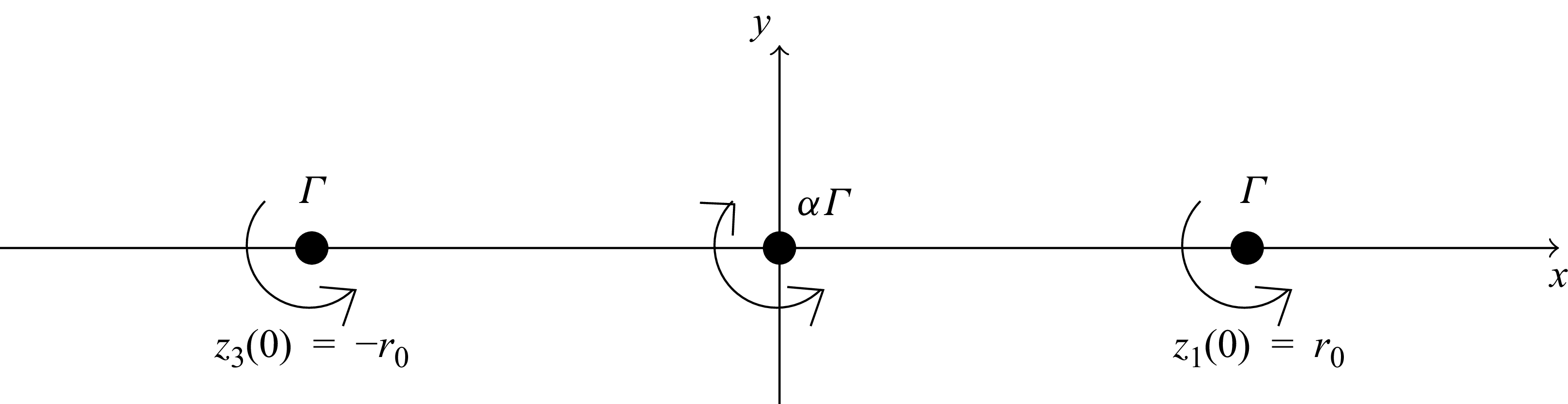


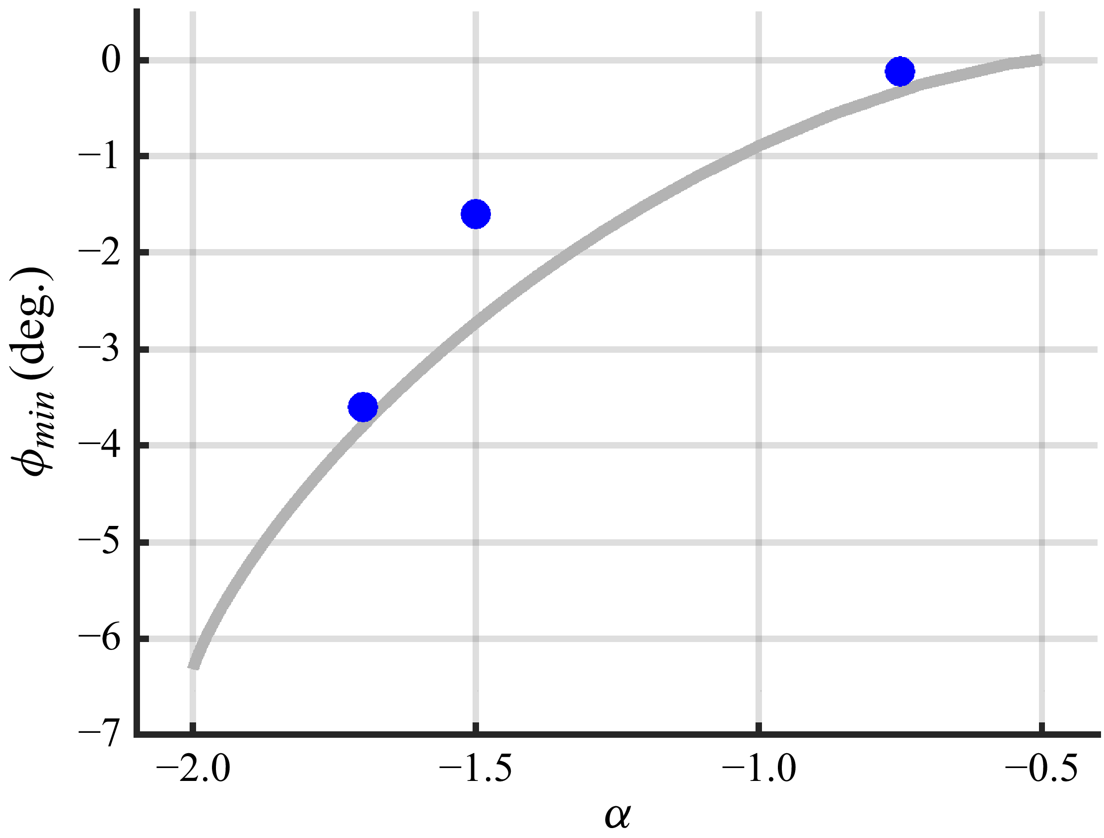


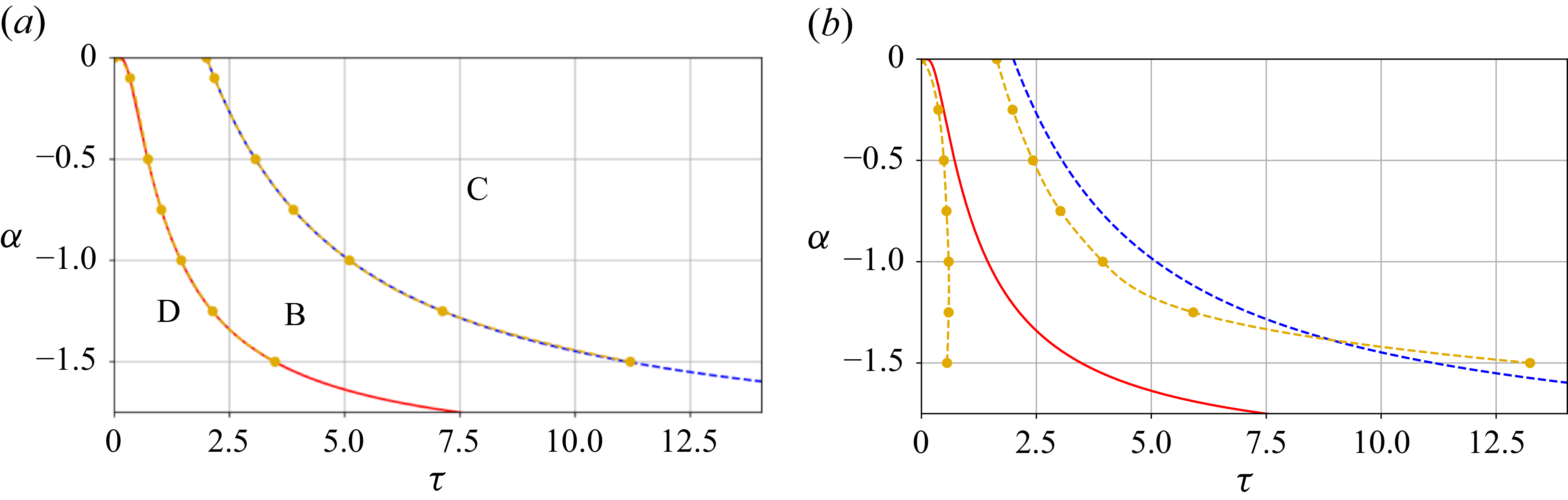


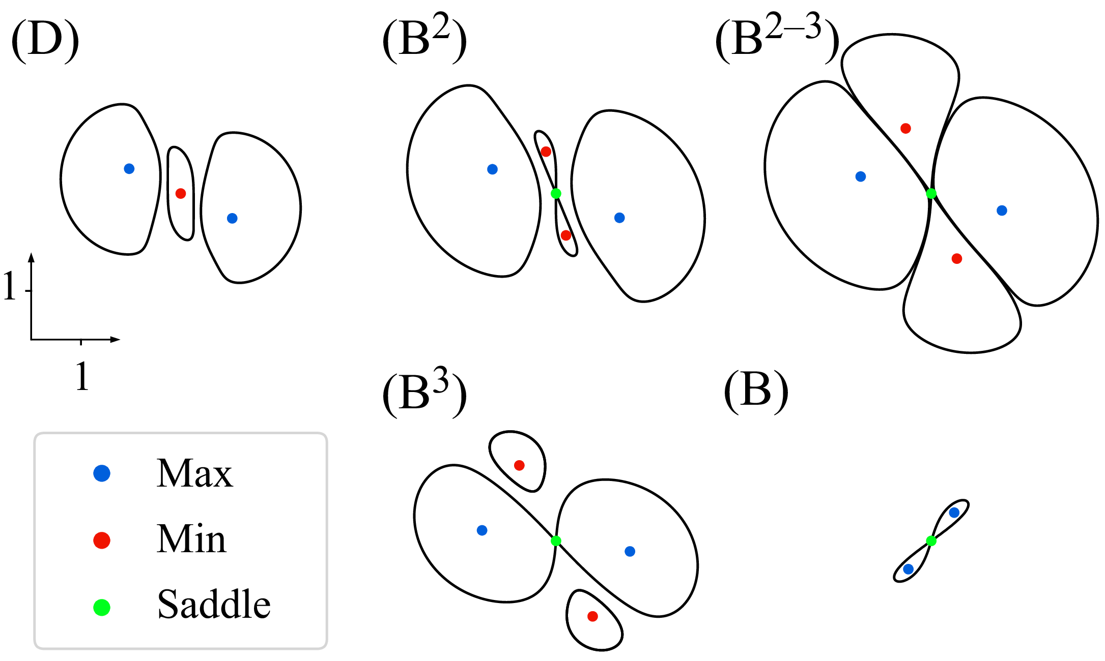


 Open access