Value of the data

• • The dataset includes both processed and raw data, the latter enabling researchers to examine the impact of new linguistic features on listener ratings

  • ○ Processed data and variables can be used immediately to conduct new analyses

  • ○ Raw data can be further processed to generate new variables to be included in additional analyses

• • The dataset includes a large and diverse sample of L1 Spanish listener-raters from five Spanish-speaking countries and a representative sample of instructed L2 Spanish learners with respect to proficiency (from two institutions of higher ed in the US)

• • A rich set of data instruments includes: two open-ended speaking tasks, transcription and rating data, a proficiency test, and detailed language learning history and experience information for both speakers and listeners

• • L2 speech data (sound files, Praat TextGrids, and transcriptions) are historically underrepresented in fields like corpus linguistics, where written data are more common; the recordings have been transcribed in CLAN so they can be easily part-of-speech tagged

• • The L2 speaker data were initially collected as part of a Registered Report (Huensch & Nagle, Reference Huensch and Nagle2021); thus, the research design underwent a peer-review process

• • L2 speech/pronunciation data from languages other than English are underrepresented in the literature (Crowther & Isbell, Reference Crowther and Isbell2024).

Background

In the field of L2 pronunciation, the past three decades have witnessed a shift away from goals of native-like attainment (or reduction of a foreign accent) toward a focus on fostering intelligible (understandable) and comprehensible (easily processed) speech. This shift was fueled by evidence that intelligibility and comprehensibility, while related to accentedness, were measurably distinct dimensions of L2 speech (e.g., Munro & Derwing, Reference Munro and Derwing1995a, Reference Munro and Derwing1995b; Derwing & Munro, Reference Derwing and Munro1997). These findings ushered in a new wave of L2 pronunciation research focused on how specific linguistic features (e.g., segmental substitutions, goodness of prosody, discourse structure) were related to (or not) each of the global dimensions (e.g., Crowther et al., Reference Crowther, Trofimovich, Saito and Isaacs2018; Isaacs & Trofimovich, Reference Isaacs and Trofimovich2012; Saito et al., Reference Saito, Trofimovich and Isaacs2016). This work has demonstrated, for example, that listener judgments of accentedness tend to be influenced by measures related to segmental (i.e., vowel/consonant errors) and word stress accuracy, whereas comprehensibility ratings are connected to a more expansive range of features, including those related to vocabulary and grammar (Crowther et al., Reference Crowther, Trofimovich, Saito and Isaacs2015b; Saito et al., Reference Saito, Trofimovich and Isaacs2016, Reference Saito, Trofimovich and Isaacs2017). At the same time, the connections among linguistic features and global speech dimensions have also been shown to be impacted by the speaking task such that in more complex tasks (i.e., completing the TOEFL iBT integrated task compared to narrating a picture story), the distinctiveness between features that differentiate accentedness from comprehensibility ratings may diminish (Crowther et al., Reference Crowther, Trofimovich, Isaacs and Saito2015a, Reference Crowther, Trofimovich, Saito and Isaacs2018). Specifically regarding comprehensibility, it appears that the speech measures of fluency and lexical richness differentiate comprehensibility ratings at the lower ends of the scale while syntactic and discourse measures better differentiate at the higher ends (e.g., Isaacs & Trofimovich, Reference Isaacs and Trofimovich2012).

To date, this body of work has contributed many important findings related to how features of a spoken utterance impact listeners’ evaluations of it. In doing so, many studies acknowledge but ultimately ignore variability among listeners by collapsing rating data to provide an average for a speaker or utterance. The intention in doing so is to focus on stimulus or speaker characteristics in an attempt to answer important questions such as: What makes a speaker comprehensible? Or what differentiates comprehensible versus accented speech for learners at different proficiency levels? Yet, we know that listeners bring their own experiences and biases to the task of communicating, and we have evidence that a variety of listener characteristics (e.g., familiarity with L2 speech, amount of teaching experience, sharing an L1) might systematically impact rater judgments (e.g., Gass & Varonis, Reference Gass and Varonis1984; Hayes-Harb et al., Reference Hayes-Harb, Smith, Bent and Bradlow2008). Despite speakers and listeners both being responsible for successful communication, research to date has often focused more on one side of this interaction, inadvertently putting the onus of communicative success on the speaker (Baese-Berk et al., Reference Baese-Berk, McLaughlin and McGowan2020; Munro, Reference Munro, Hansen and Zampini2008).

The current dataset, with its diverse sample of L1 Spanish listeners from five Spanish-speaking countries and rich set of data instruments, has the potential to directly contribute to a better understanding of which factors of a listener’s background influence speech ratings. Datasets that include speech data, in particular those that have been transcribed and annotated, are relatively rare because they can be expensive and time-consuming to compile (Huensch & Staples, Reference Huensch, Staples, Derwing, Munro and Thomson2022). L2SLRD represents such a dataset and is presented with detailed and thorough documentation, which would allow for additional data to be added in the future. Finally, like many other subfields in SLA, the majority of research in L2 pronunciation has focused on L2 English as a target (e.g., Thomson & Derwing, Reference Thomson and Derwing2015). Although this trend appears to be improving (Chau & Huensch, Reference Chau and Huensch2025), the current dataset responds to recent calls for an increased focus on languages other than English (Crowther & Isbell, Reference Crowther and Isbell2024; Levis, Reference Levis2021) as the data involve listeners and speakers of Spanish.

Data description

The data are publicly available online at https://osf.io/67nm4/ with full documentation (see Appendix A of the Supplementary Material for the L2SLRD OSF README) and consist of:

L1 listener rating data (n = 201) Footnote ¹

• • Biographical data for all listeners including information about language learning history and experience with learner speech;

• • n = 80 listeners from five Spanish-speaking countries transcribed and rated comprehensibility and accentedness for the Hunter story utterances (Huensch & Nagle, Reference Huensch and Nagle2021);

• • n = 80 listeners from five Spanish-speaking countries transcribed and rated comprehensibility and accentedness for the Vacation utterances (Huensch & Nagle, Reference Huensch and Nagle2023);

• • n = 60 listeners from four Spanish-speaking countries rated comprehensibility and accentedness for the Hunter story utterances (no transcription; not previously published);

• • n = 49 listeners from four Spanish-speaking countries rated comprehensibility and accentedness for the Vacation utterances (no transcription; not previously published).

All listeners were recruited and completed tasks through Amazon Mechanical Turk (AMT).

L2 speaker data ^{Footnote 2} (n = 42)

• • Oral proficiency data: elicited imitation recordings, transcripts (in Excel), and scores;

• • Biographical data including information about language learning history and experience;

• • Speech recordings from a picture description task (Hunter story, Munro & Derwing, Reference Munro and Derwing1995a) and an open-ended response to a prompt based on NCSSFL-ACTFL Can-Do statements ( Describe un lugar que hayas visitado o que te interese visitar y explica por qué fuiste o por qué quieres ir a ese lugar “Describe a place you have visited or are interested in visiting and explain why you went there or why you might want to go to this place.”) (Vacation);

  • ○ Both the full recordings (approximately one minute each) and the processed, selected utterances used for the listener rating task are provided as wav files;

  • ○ Syllable counts for all selected utterances (Hunter story and Vacation) are included in the “syllables” column of the “data—all variables public.csv” datasheet;

  • ○ Phonemic and grammar error counts and goodness of prosody ratings are included for the Hunter story (but not the Vacation) utterances.

• • Transcripts (following CHAT guidelines in CLAN, MacWhinney, Reference MacWhinney2000) of the oral recordings for two utterances (each approximately nine words in length) from each speaker.

Selected results

The first data collection wave of the L2SLRD was conducted as part of a registered report (Huensch & Nagle, Reference Huensch and Nagle2021) investigating intelligibility, comprehensibility, and accentedness in L2 Spanish and the potential impacts of L2 proficiency on the relationships among those global speech dimensions. The study included collecting data from all speakers and the first wave of listeners. The speakers were 42 L2 learners of Spanish of varying proficiency from two institutions in the US. They completed a variety of tasks, including oral recordings of both a picture story retell (i.e., the Hunter story) and an open-ended response to a prompt based on NCSSFL-ACTFL Can-Do Statements (i.e., Vacation). For the registered report analysis, two short utterances (approximately nine words) were extracted from the Hunter story recordings and presented to L1 Spanish listeners (n = 80) from five different countries (Argentina, Colombia, Mexico, Spain, and Venezuela). The listeners transcribed the utterances and rated them for comprehensibility and accentedness. The utterances were also coded for a variety of linguistic features including pronunciation errors, lexico-grammatical errors, speech rate, and goodness of prosody. Similar to findings from L2 English (Derwing & Munro, Reference Derwing and Munro1997; Munro & Derwing, Reference Munro and Derwing1995a), the results showed that comprehensibility was more aligned with intelligibility than accentedness was: For every one standard deviation increase in comprehensibility, an utterance was twice as likely to be intelligible (relative to the base odds), whereas accentedness was not a significant predictor of intelligibility. As in Munro and Derwing’s work, listeners varied in terms of how strongly related their comprehensibility and accentedness ratings were. There was also some evidence that listeners assigned different weights to different linguistic features across the proficiency continuum, leading Huensch and Nagle to conclude that “research in the field has only begun to skim the surface of sources of variance in the listener-based constructs” (p. 660).

Building on Huensch and Nagle (Reference Huensch and Nagle2021), two additional studies were published: one reporting on phonetic predictors of the global dimensions (Nagle et al., Reference Nagle, Huensch and Zárate-Sández2023) and the other, the potential impact of the speaking task (Huensch & Nagle, Reference Huensch and Nagle2023). Nagle et al. did not collect additional data but rather used the existing Hunter story utterances for a phonetic analysis of pronunciation features that previous research had found to be difficult for English L1 learners (e.g., rhotics, diphthongization, stop consonant voice onset time). While a variety of phonetic features were associated with accentedness, very few were associated with either comprehensibility or intelligibility. Huensch and Nagle (Reference Huensch and Nagle2023) conducted a second wave of listener data collection to examine whether the speaking task impacted listener judgments (n = 80) of the global speech dimensions. That study had a similar design to Huensch and Nagle (Reference Huensch and Nagle2021) except that the utterances rated by listeners came from the open-ended response (i.e., Vacation task). There were minimal differences in outcomes compared to the analysis that included the Hunter story utterances. A third wave of data collection was undertaken to elicit comprehensibility and accentedness ratings of the Hunter story and Vacation utterances without having listeners complete a transcription task. Other than in this data report, this data has not been reported on in a published study.

A clear takeaway from previous findings using the L2SLRD is that, like Munro and Derwing (Reference Munro and Derwing1995a) and Derwing and Munro (Reference Derwing and Munro1997) (and similar studies) both Huensch and Nagle studies reported “substantial variation in the strength of the relationship between the listener-based dimensions [i.e., accentedness and comprehensibility]” (Huensch & Nagle, Reference Huensch and Nagle2021, p. 656), indicating the need for additional research to better understand factors contributing to this variation on many fronts. In the following, a more detailed description of the experimental design, materials, and methods is provided, after which dataset descriptives are presented. This is followed by a discussion of potential avenues for future research both in the short and long term using this dataset.

Experimental design, materials, and methods

The L2SLRD Coding and Experimental Protocols PDF in the Documentation folder on the OSF contains all of the protocols for the dataset. In this section, page numbers refer to that document. Speaker data were collected in person between October 2019 and March 2020 following the Experimental Protocol (pp. 1–10). The order of the tasks was randomized for each participant (pp. 47–66). After these data were collected, they were processed and coded following the registered report Data Processing Workflow (p. 46). Listener data were collected in three waves via AMT: (a) Hunter story transcriptions and ratings were collected between April and June 2020 (published in Huensch & Nagle, Reference Huensch and Nagle2021), (b) Vacation utterance transcriptions and ratings were collected between June and August 2021 (published in Huensch & Nagle, Reference Huensch and Nagle2023), and (c) Hunter story and Vacation utterance ratings (without transcription) were collected between May 2023 and March 2024 (unpublished).

Data preparation and coding

Recordings of semi-spontaneous speech were first transcribed orthographically in CLAN following CHAT conventions (see Transcription Protocol, pp. 38–45). After transcripts were checked, two coders independently selected utterances from the transcripts following the Protocol for Selecting Utterances (p. 19). That protocol provided detailed instructions for selecting viable utterances using information such as phrase/clause boundaries, pausing characteristics, and intonation contours and offered inclusion/exclusion criteria based on utterance length and the use of English words. The selections were compared, and any differences were identified and resolved (see utterance selection spreadsheets provided in the task subfolders of the Speaker Data folder on the OSF). Utterances were tagged in CLAN to allow for automatic extraction, and initial hesitations (e.g., um, eh, y “and”) were tagged to be ignored (pp. 22–24). Once tagged, the chat2praat command in CLAN was used to create Praat TextGrids which provided rough utterance-level segmentation based on the time stamps/bullets in the CHAT transcript. These TextGrids were modified for the final analysis by manually aligning segmentation boundaries and removing non-analyzed utterances (see Protocol to Code Utterances in CLAN and Segment Utterances in Praat, p. 24). A Praat script was used to extract the utterances as .wav files to be used as stimuli for the listener rating task (see Praat Scripts folder in Documentation folder on the OSF). Basic fluency data were gathered using CLAN commands on the transcripts (see Protocol to Process Transcripts once Utterances selected, pp. 22–24), and sound files and transcripts were anonymized following the Protocol for Anonymizing Files (pp. 12–13). For the Hunter story utterances only, a final coding step was taken. Once the previous steps were completed, syllables were counted using the Protocol for Counting Syllables, phonemic errors were coded using the Protocol for Coding Phonemic Errors, grammatical errors were coded using the Protocol for Coding Grammatical Errors, and prosody was rated using the Protocol for Rating Goodness of Prosody (pp. 16, 15, 14, and 18, respectively). This coding was not completed for the Vacation utterances.Footnote ³

The elicited imitation tests were first transcribed (see Protocol for EIT transcription, p. 17). Next, they were rated following standard procedures for the elicited imitation test: Each utterance received a score on a scale of 0–4, with 0 indicating no response or an isolated word and 4 indicating exact repetition.

Listener transcriptions were coded for intelligibility scores using the Transcription Coding Protocol (pp. 25–35). Each utterance was coded in an Excel worksheet (see Figure 1). Each worksheet included a column indicating the final, decided-upon utterance and a column for the coder transcription. Underneath the decided-upon utterance coding was a row of EMs (referring to exact match), with each EM code corresponding to a word in the utterance. If the utterance was transcribed 100% correctly by the listener, the row of EMs was copy/pasted. In the case of any differences, the EM code was replaced with a new code such as T for “trivial error,” O for “omission,” and so forth.

Figure 1.

Example of transcription coding in Excel.

Dataset descriptives

The main data files are provided in the Listener Data and Analysis Code folder on the OSF along with a codebook and include (a) data—listener demographics public.csv = just the listener demographic data, (b) data—all variables public.csv = complete data file. The analysis code for analyses presented in the current report is also included in that folder: L2SLRD code.Rmd = markdown with the code needed to reproduce tables, plots, and analyses (and L2SLRD code.html). Previously reported analyses (csv files and analysis code) are included in the Published Analyses folder on the OSF. Appendix C of the Supplementary Material provides a single, consolidated overview table summarizing counts across tasks and conditions (e.g., speakers, utterances, listeners, ratings).

As a means of presenting the data in an analysis-neutral way, we computed descriptive information for the data in two ways: Table 1 presents listener demographics by task and transcription status, and Table 2 presents listener demographics by country of origin.

Table 1.

Listener demographics by task (hunter, vacation) and transcription (with, without).

Table 1. Long description

The table is organized into four columns representing listener groups: Hunter with transcription (n equals 80), Hunter without transcription (n equals 60), Vacation with transcription (n equals 80), and Vacation without transcription (n equals 49).

Continuous variables (mean and standard deviation):

* Age: Ranges from 32.91 to 38.13.

* A O Spanish: Ranges from 0.02 to 0.57.

* A O English: Ranges from 7.11 to 8.53.

* Prof. Spanish: Ranges from 8.78 to 8.88.

* Prof. English: Ranges from 6.80 to 7.24.

* percent Daily Spanish: Ranges from 79.14 to 83.33.

* percent Daily English: Ranges from 15.16 to 19.08.

* percent Daily other: Ranges from 1.85 to 17.29.

* Familiarity: Ranges from 6.39 to 6.83.

Count variables (frequency and percentage):

* Frequency of interaction: Most participants interact monthly (37 percent to 53 percent).

* Context: Personal interaction is highest in the Hunter with group (53 percent) and lowest in the Vacation without group (16 percent). Professional interaction ranges from 42 percent to 50 percent.

* Linguistics training: Present in 46 percent to 60 percent of participants.

* Teaching experience: Present in 16 percent to 21 percent of participants.

Note: AO = Age of onset; Context = context of interaction with L2 Spanish speakers; Familiarity = self-reported familiarity with L2 Spanish speech; Frequency = frequency of interaction with L2 Spanish speakers; Linguistics = linguistic training; Prof. = self-reported global proficiency, created by taking the average of ratings provided for speaking, listening, reading, and writing; Teaching = language teaching experience.

Table 2.

Listener response demographics by country of origin.

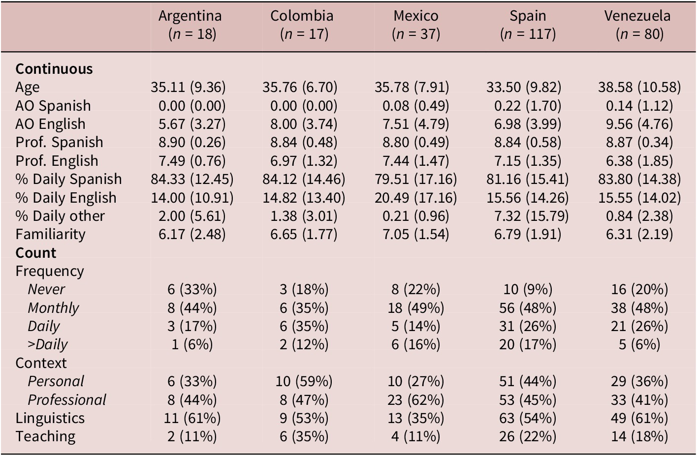
Table 2. Long description

The table is organized into five columns by country: Argentina (n equals 18), Colombia (n equals 17), Mexico (n equals 37), Spain (n equals 117), and Venezuela (n equals 80).

Continuous variables (mean and standard deviation):

* Age: Ranges from 33.50 in Spain to 38.58 in Venezuela.

* A O Spanish: Near zero for all groups (0.00 to 0.22).

* A O English: Ranges from 5.67 in Argentina to 9.56 in Venezuela.

* Prof. Spanish: High across all groups, averaging approximately 8.8 to 8.9.

* Prof. English: Ranges from 6.38 in Venezuela to 7.49 in Argentina.

* Percent Daily Spanish: High across all groups, ranging from 79.51 percent in Mexico to 84.33 percent in Argentina.

* Percent Daily English: Ranges from 14.00 percent in Argentina to 20.49 percent in Mexico.

* Familiarity: Self-reported familiarity with L 2 Spanish speech ranges from 6.17 to 7.05.

Count variables (frequency and percentage):

* Frequency of interaction: Most participants across all countries report ‘Monthly’ interaction (ranging from 35 percent to 49 percent).

* Context of interaction: ‘Professional’ context is highest in Mexico (62 percent), while ‘Personal’ context is highest in Colombia (59 percent).

* Linguistics training: Reported by 61 percent in Argentina and Venezuela, 53 percent in Colombia, 54 percent in Spain, and 35 percent in Mexico.

* Teaching experience: Ranges from 11 percent in Argentina and Mexico to 35 percent in Colombia.

Note: AO = Age of onset; Context = context of interaction with L2 Spanish speakers; Familiarity = self-reported familiarity with L2 Spanish speech; Frequency = frequency of interaction with L2 Spanish speakers; Linguistics = linguistic training; Prof. = self-reported global proficiency, created by taking the average of ratings provided for speaking, listening, reading, and writing; Teaching = language teaching experience.

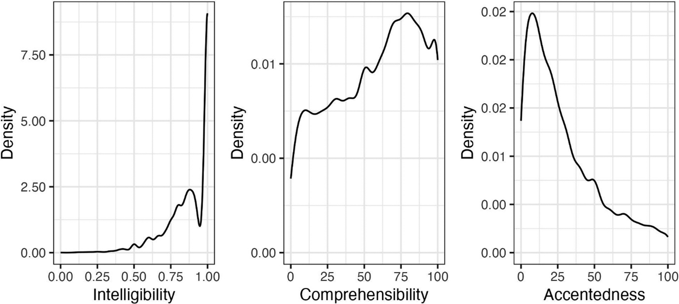
Figure 2 shows the distribution (density) of intelligibility, comprehensibility, and accentedness scores for L2 speakers, pooling over tasks (hunter and vacation) and transcription (with and without the transcription task for comprehensibility and accentedness). As shown, intelligibility scores were very heavily skewed toward perfect intelligibility, which was in fact the most common score. Scores below 0.75 were uncommon, and there were few scores below 0.50. Comprehensibility scores were also skewed toward higher levels of comprehensibility, but the distribution was more uniform, with scores observed throughout the 100-point scale. Accentedness showed the opposite pattern, with scores heavily skewed toward the lower end of the continuum, though like comprehensibility, scores were observed throughout the scale. Taken together, the plots suggest that most utterances were highly intelligible, moderately to highly comprehensible, and strongly to moderately accented.

Figure 2.

Density plots for intelligibility, comprehensibility, and accentedness.

Note: Constructs have unique density scales determined by their score distribution.

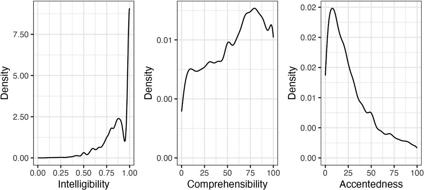
Figure 2. Long description

The figure consists of three panels arranged horizontally.

Panel 1, Intelligibility. The x-axis ranges from 0.00 to 1.00 and the y-axis represents Density from 0.00 to 7.50. The data curve remains near zero until 0.50, then shows small fluctuations before a sharp, nearly vertical increase peaking at the maximum value of 1.00.

Panel 2, Comprehensibility. The x-axis ranges from 0 to 100 and the y-axis represents Density from 0.00 to 0.01. The curve rises quickly from 0, plateaus with minor peaks around 25 and 50, and reaches its highest peak between 75 and 80 before a slight decline toward 100.

Panel 3, Accentedness. The x-axis ranges from 0 to 100 and the y-axis represents Density from 0.00 to 0.02. The curve rises sharply to a peak at approximately 10 on the x-axis, then follows a steady, asymptotic decline toward the right, reaching its lowest density at 100.

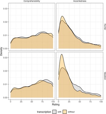
Figure 3 shows the comprehensibility and accentedness plots faceted by task (hunter vs vacation, shown in rows) and transcription status (with vs without transcription, mapped to color). As displayed, the density plots are highly similar, save for accentedness, where accentedness scores tended to be even more skewed toward the lower end of the continuum when the rating task was not accompanied by transcription.

Figure 3.

Density plots for comprehensibility and accentedness ratings by task and transcription.

Note: Each rating has a unique density scale.

Figure 3. Long description

The multi-panel plot is organized into a two-by-two grid. The columns are labeled Comprehensibility and Accentedness. The rows are labeled Hunter and Vacation. The x-axis for all panels represents Rating from 0 to 100. The y-axis represents Density from 0.00 to 0.03. A legend at the bottom indicates that grey areas represent with transcription and tan areas represent without transcription.

* Top-Left Panel (Hunter, Comprehensibility): Both curves are relatively flat and broad, peaking between ratings of 75 and 90. The with and without transcription curves closely overlap.

* Top-Right Panel (Hunter, Accentedness): Both curves show a sharp peak at the lower end of the scale, around a rating of 10. The without transcription curve has a slightly higher peak density of approximately 0.025 compared to the with transcription curve at 0.021.

* Bottom-Left Panel (Vacation, Comprehensibility): Similar to the Hunter task, these curves are broad with a gradual increase, peaking near a rating of 80. The with transcription curve shows a slightly higher density peak at the far right of the scale.

* Bottom-Right Panel (Vacation, Accentedness): Both curves show a very high, narrow peak near a rating of 10. The without transcription curve reaches a significantly higher peak density of approximately 0.032, while the with transcription curve peaks lower at 0.022 and shows a secondary small bulge around a rating of 45.

Potential uses

Example use

As stated previously, results from earlier waves of the L2SLRD indicated variation in the strength of the relationship between some of the listener-based dimensions. Specifically, the relationship between accentedness and comprehensibility varied across the listeners, but the relationship between comprehensibility and intelligibility did not (Huensch & Nagle, Reference Huensch and Nagle2021, p. 656). This and similar findings (Chau & Huensch, Reference Chau and Huensch2025; Huensch & Nagle, Reference Huensch and Nagle2023) led us to be interested in the extent to which the comprehensibility and accentedness ratings, and their correlation, varied based on whether the listeners transcribed the utterance (i.e., whether the listeners engaged in an intelligibility evaluation task).

Data wrangling, visualization, and analysis were carried out in R version 4.5.3 (R Core Team, 2026). We fit a Bayesian zero/one-inflated beta (ZOIB) regression model using the brms package (version 2.22.0; Bürkner, Reference Bürkner2021). We chose this model because comprehensibility can be conceptualized as bounded between 0 and 1 (comprehensibility/100), and both 0 and 1 were attested in the data (6.70% of the data were 0 or 1; 1.21% were 0 and 5.49% were 1). In a ZOIB model, a logistic regression predicts 0s and 1s in the data (α), another logistic regression predicts whether 0s and 1s are 1s (γ), and a beta regression (defined by two shape parameters: μ and ϕ) predicts the mean and precision (distribution) with respect to the rest of the scale not defined by 0 and 1. All parameters are on the logit scale, save the precision parameter ϕ, which is on the log scale (for more information on beta and ZOIB regression, see Corretta & Bürkner, Reference Corretta and Bürkner2025; Heiss, Reference Heiss2021).

We included transcription in all model components to predict whether the presence of a transcription task affected the probability of observing a 0 or 1 (α), the probability of a 1 (γ), and the mean and distribution of scores in the 0–1 range, excluding 0 and 1. Put another way, we were interested in the extent to which the transcription task affected the probability of observing extreme scores (0 and 1), the average comprehensibility score (μ), and the distribution of scores (ϕ). We included accentedness only in the beta regression portion of the model, allowing it to predict μ but not the other model parameters. We also included an interaction between transcription and accentedness, again only in the beta regression portion and only in relation to μ. We made these choices to limit model complexity to the extent possible while also ensuring we were able to fully model the impact of the transcription task on comprehensibility. We used treatment coding for transcription, setting the reference level to “with transcription” to align with our previous analyses, and we standardized accentedness. We included by-listener and by-fileFootnote ⁴ random intercepts across the model (α, γ, μ, and ϕ). For the beta regression component, we included by-listener random slopes for accentedness and by-file random slopes for accentedness, transcription, and the interaction.

We used weakly informative priors, save for the prior for accentedness, pushing the average toward a positive value based on previous research demonstrating such an effect: normal(0.2, 0.3) instead of normal(0, 0.3). Full information on the priors, including prior predictive checks, is available in the accompanying analysis code. We ran the model with 12,000 iterations, of which 2,000 were warmup. R-hat values and effective sample size were within acceptable thresholds (R-hat < 1.05, ESS > 0.1), and trace plots showed the expected fuzzy caterpillar pattern. We also ran posterior predictive checks, which showed that the model-generated distributions approximated the observed distribution well. To limit the complexity of presentation, here we focus on μ rather than the other model parameters. Information on the other parameters can be obtained from the code.

For ease of interpretation, we back-transform from the log odds that the model outputs to estimated comprehensibility scores on the original 100-point scale. For estimated differences by transcription, we report odds ratios. On the odds ratio scale, values above 1 increase comprehensibility and values below 1 decrease it relative to the baseline odds. We use the posterior distribution of each effect to summarize its mean and its 95% and 80% credible intervals (CredIs). The credible interval represents the probability with which the estimate falls within the interval, so an 80% interval would mean we can be 80% confident that the interval contains the estimate.

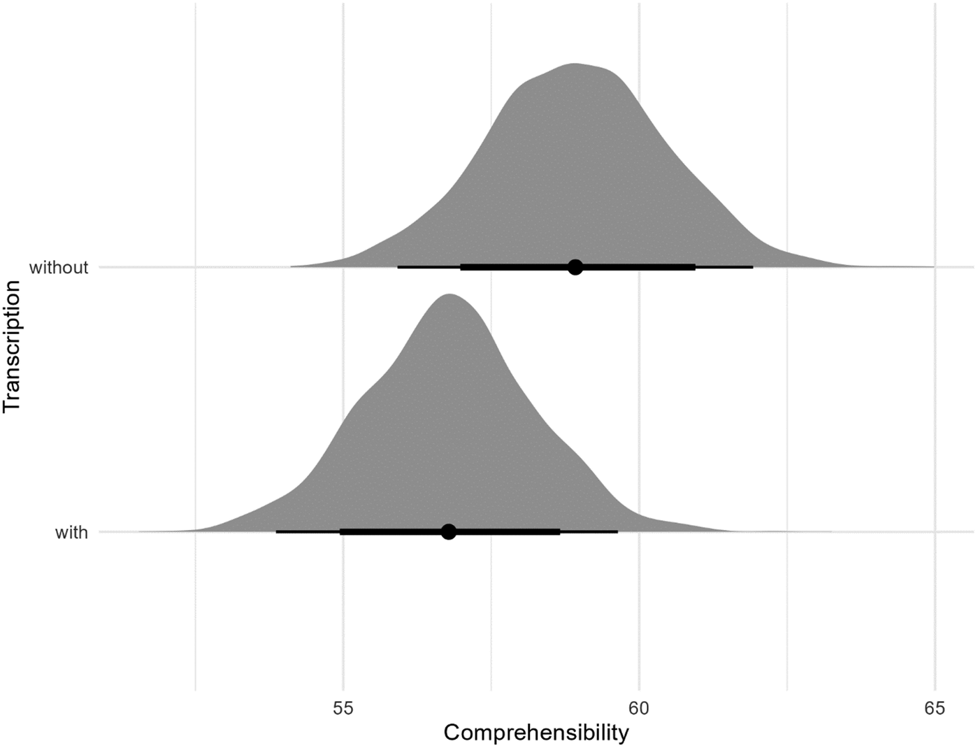
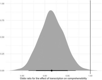
As a first step, we examined the point estimates and CredIs for the ratings with and without transcription. For the ratings with transcription, b = 0.273 logits (95% CredI [0.155, 0.390], 80% CredI [0.198, 0.350]). For the ratings without transcription, the estimate was slightly higher, b = 0.362 logits (95% CredI [0.238, 0.486], 80% CredI [0.281, 0.445]). As shown in Figure 4, this equates to an estimated average comprehensibility score of 57 with transcription and 59 without. Figure 5 plots the posterior distribution of the difference in scores as an odds ratio (with–without transcription). On this plot, an odds ratio <1.00 indicates a positive effect of transcription on comprehensibility (i.e., comprehensibility scores are higher when transcription is included) and an odds ratio >1.00 indicates a negative effect (i.e., comprehensibility scores are higher when transcription is not included). Based on this plot, we can be confident that including a transcription task decreases comprehensibility ratings because nearly the entire distribution falls below 1.00. The 95% and 80% CredIs for the difference were [0.86, 0.97] and [0.88, 0.95], respectively. Considering both intervals, we can be somewhat confident that including a transcription task decreases comprehensibility by about 5–10% (relative to the base comprehensibility, or 5–10% of 59). Given the relatively high comprehensibility baseline, this is a rather small effect.

Figure 4.

Posterior distribution of comprehensibility scores by transcription.

Figure 4. Long description

The graph features a horizontal x-axis labeled Comprehensibility with numerical markers at 55, 60, and 65. The vertical y-axis is labeled Transcription and contains two categories: without and with.

At the top, the without category shows a grey density curve centered further to the right. A black horizontal interval bar sits below the curve, with a central dot indicating a median score of approximately 59. The thick part of the interval bar spans from roughly 57 to 61, while the thinner whiskers extend from 56 to 62.

Below it, the with category shows a grey density curve shifted to the left. Its central dot indicates a lower median score of approximately 57. The thick interval bar for this group spans from roughly 55 to 59, with thinner whiskers extending from 54 to 60.

The distribution for without is generally higher on the comprehensibility scale compared to the distribution for with.

Figure 5.

Posterior distribution of comprehensibility difference with vs. without transcription.

Note: 1.00 = no effect/no change in comprehensibility. OR > 1.00 indicates higher scores with transcription. OR < 1.00 indicates higher scores without transcription.

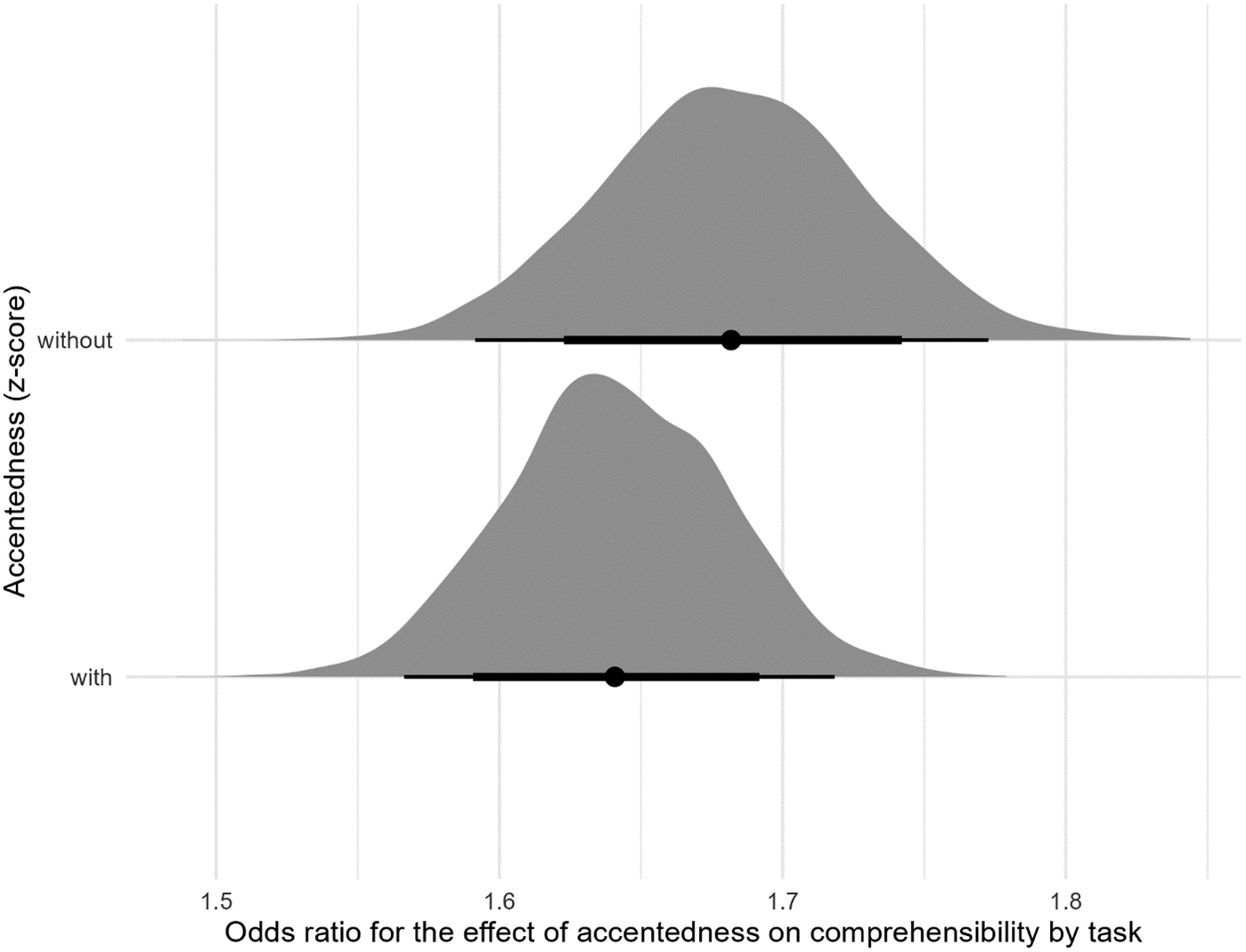
Figure 6 plots the posterior distribution of the effect of accentedness on comprehensibility with and without transcription. The point estimate and CredIs for accentedness were 0.495 logits (95% CredI [0.449, 0.541], 80% CredI [0.464, 0.526]) with transcription and 0.520 logits (95% CredI [0.465, 0.572], 80% CredI [0.484, 0.555]) without transcription. For a file 1 SD above the mean level of accentedness on a task with transcription (+ 0.495 logits), this would amount to an increase in comprehensibility of 64% (odds ratio = 1.64) relative to the base odds (0.273 logits). In terms of comprehensibility, an utterance 1 SD above the mean accentedness score would be predicted to have a comprehensibility score of 68. For a similar file on a task without transcription, this would mean an increase of 68% and would translate to a comprehensibility score of 71. Figure 7 plots the difference in the effect of accentedness on comprehensibility by task. This difference plot can be interpreted in the same way as the difference plot for transcription (Figure 4): odds ratios > 1.00 indicate a stronger effect of accentedness on comprehensibility when transcription is included and odds ratios < 1.00 indicate a weaker effect. From these plots, we can see that the effect of accentedness on comprehensibility was positive, but the difference in the relationship between the two constructs as a function of transcription was negligible. In the difference plot, although most of the distribution is < 1.00, indicating a stronger relationship when transcription is included, a sizable portion is > 1.00, which means the directionality of the effect is uncertain. Moreover, the effect is quite small (odds ratio = 0.98, 95% CredI [0.93, 1.03], 80% CredI [0.94, 1.01]).

Figure 6.

Posterior distribution of accentedness odds ratios by transcription.

Figure 7.

Posterior distribution of accentedness difference with vs. without transcription.

Note: 1.00 = no effect/no change in comprehensibility. OR > 1.00 indicates a stronger effect of accentedness on comprehensibility with transcription. OR < 1.00 indicates a weaker effect of accentedness on comprehensibility without transcription.

Figure 8 visualizes all three effects simultaneously. As shown, comprehensibility is slightly lower when transcription is included (left panel) compared to when it is not (right panel), the relationship between accentedness and comprehensibility is positive, and the lines in both panels are virtually parallel, suggesting a similar relationship between the two constructs regardless of transcription. Put another way, a transcription task appears to have a subtle yet consistent effect on comprehensibility, such that scores are slightly lower when listeners transcribe files, but the effect of transcription on the relationship between accentedness and comprehensibility is practically negligible.

Figure 8.

Relationship between accentedness and comprehensibility by transcription.

Finally, we summarize the random effects, focusing on by-listener variance in the effect of accentedness and by-file variance in the effect of transcription. The by-listener SD for accentedness was 0.079 log odds. When added to the fixed effect (0.495 ± 2 × 0.079) and converted to odds ratios through exponentiation, 95% of listeners should fall between 1.40 and 1.92. Put another way, for nearly all listeners, the relationship is expected to be positive. The by-file SD for the transcription difference was 0.148 log odds, whereas the fixed effect was just half that at 0.089. Following the same steps of combining the fixed and random effects and exponentiating to get the odds ratio, for 95% of utterances of this type, the difference would be expected to fall between 0.81 and 1.47. The effect of transcription was therefore highly variable at the level of individual files. Although the mean effect favored the absence of transcription—files received higher comprehensibility ratings on average when they were not accompanied by a transcription task—for some files, the opposite could be true, and for others, no effect would be expected at all.

Figure 9 plots the random effects. The by-listener effects are shown in the left panel and the by-file effects in the right panel. The solid black lines represent the fixed effect ± 2 SD (i.e., where 95% of listeners would be expected to fall), and the red line represents odds ratio = 1.00 (no effect). To make the plot easier to read, we have removed the file and listener labels, and we plot point estimates rather than points and credible intervals. As shown, for listeners, the relationship between accentedness and comprehensibility was consistently positive (odds ratios > 1.00) but variable in magnitude, whereas at the file level, the relationship between transcription and comprehensibility varied in both directionality (most odds ratios <1.00, but some >1.00) and magnitude, and a null effect was clearly possible.

Figure 9.

By-listener and by-file random effects.

Note: Red line is shown at odds ratio = 1.00 (no effect). Black lines indicate boundaries at ± 2 SD (fixed effect ± 2 × SD of random effect estimate).

Figure 9. Long description

The image consists of two side-by-side panels.

Left Panel:

- The x-axis is labeled By-listener variability in accentedness with values from 1.0 to 3.5.

- The y-axis is labeled Listener.

- A red vertical line is positioned at 1.0.

- Two black vertical lines are positioned at approximately 1.4 and 1.9.

- Black data points form a dense, upward-sloping S-curve starting at 1.0 on the bottom left and extending to 3.5 at the top right. Most points are clustered between the two black lines.

Right Panel:

- The x-axis is labeled By-file variability in transcription with values from 0.7 to 1.5.

- The y-axis is labeled File.

- A red vertical line is positioned at 1.0.

- Two black vertical lines are positioned at approximately 0.8 and 1.45.

- Black data points form a similar upward-sloping S-curve starting at 0.7 on the bottom left and extending toward 1.2 at the top right. The curve crosses the red line at 1.0 near the upper-middle section of the plot.

Recommendations and conclusions

We close this data report with a brief discussion of strategies for researchers interested in sharing data publicly in the future and share several challenges we encountered along the way in preparing to share the current dataset.

Whether one is sharing data for an individual manuscript in support of open science initiatives (Liu et al., Reference Liu, Chong, Marsden, McManus, Morgan-Short, Al-Hoorie, Plonsky, Bolibaugh, Hiver, Winke, Huensch and Hui2023) or intending to curate a dataset such as the L2SLRD, several strategies can be implemented to facilitate the process. One of the most critical components is detailed planning and thorough documentation. The initial data collection wave of the L2SLRD benefited from being planned as a registered report and multisite study. These two aspects necessitated advanced planning and clear documentation: The study design and methods were scrutinized as part of the registered report peer review process, and simultaneous data collection at two different sites resulted in meticulously detailed protocol documents. Datasets such as this one are typically built over several rounds of data collection, which can span months or years. Creating readme files or other sorts of documentation with information about what is shared, where, and how can streamline data aggregation by providing a clear trail of documentation during the lifespan of the project. If some of this sounds overwhelming, another consideration is that sharing data is not an all-or-nothing venture. Researchers can start small by simply sharing the aggregated data (e.g., csv file) and analysis code needed to reproduce an analysis in a published study. This can be followed by “leveling up” to share additional pieces such as cleaned data, coding protocols, and more. A recent addition to our own workflow has been harnessing the affordances of the GitHub platform to more efficiently manage version control and document decision-making.

Some challenges we have faced while preparing the L2SLRD include both selecting what to share and managing changes in technologies over the years. As one can see in the experimental protocol, not all of the data collected as part of the registered report were shared as part of this dataset. We made every effort to be comprehensive while at the same time avoiding sharing an overwhelming amount of information. Over the course of a project that spans seven years, changes in technology are inevitable. We have changed institutions, and our institutions have migrated from Dropbox to Box or OneDrive. Likewise, R packages have undergone updates or become obsolete. These types of changes are minor and expected and therefore relatively easy to adapt to, at least in our experience. Changes to personnel can be more impactful because special consideration must be given to onboarding and training (and also to documenting changes in training protocols over the lifecycle of the project). Yet another example is the fact that we could not collect data from Venezuela for the no-transcription tasks due to a change in IRB policy.

Perhaps most importantly and obviously, our own project management and data analysis practices have evolved (and hopefully improved) over time. Although these changes are positive, they also affect how things have been stored and managed. As one practical example, the variables included in the base datasets were slightly different, which in some cases required us to rebuild the data from scratch, returning to the original AMT files. This step was necessary for creating parallel datasets that could then be aggregated into the final, comprehensive dataset we report here. Ultimately, this step was the most time-consuming. Thus, we can also recommend that if researchers are interested in possible data sharing, they adopt a single, common data structure that they use throughout all iterations of the project. Ideally, this data should be as comprehensive as possible, reflecting current use as well as any that could be envisioned in the future (within reason), to make future compilation and sharing easier. As with all open science practices, the investments you make in planning and documentation now pay future dividends.