


1 Introduction
The Kármán vortex street is a never-ending source of fascination for the fluid dynamicist. As fluid passes a bluff body, the vorticity created at the surface organises itself into shear layers. These layers subsequently break up into individual vortices which move downstream with the flow. The vortex street thus created is highly organised and typically consists of two sequences of vortices, one from each side of the body, with circulations of opposite signs (Benard Reference Benard1908a
,Reference Benard
b
; von Kármán Reference von Kármán1912). Depending on the shape and motion of the body more complicated patterns of vortices may arise (Williamson & Roshko Reference Williamson and Roshko1988; Ponta & Aref Reference Ponta and Aref2006; Schnipper, Andersen & Bohr Reference Schnipper, Andersen and Bohr2009). Being ubiquitous in nature and technology, the Kármán vortex street has been extensively studied, in particular when the bluff body is a circular cylinder, the case we shall also consider here. The basic steps in the formation of the vortex street as the Reynolds number increases are well known. Defining $Re=UD/\unicode[STIX]{x1D708}$
where
$Re=UD/\unicode[STIX]{x1D708}$
where $U$
is the speed of the uniform incoming flow,
$U$
is the speed of the uniform incoming flow, $D$
is the diameter of the cylinder and
$D$
is the diameter of the cylinder and $\unicode[STIX]{x1D708}$
is the kinematic viscosity of the fluid, one finds that for
$\unicode[STIX]{x1D708}$
is the kinematic viscosity of the fluid, one finds that for $Re<Re_{S}\approx 5$
the flow is steady and attached to the cylinder. At
$Re<Re_{S}\approx 5$
the flow is steady and attached to the cylinder. At $Re_{S}$
the flow separates and two symmetric recirculation zones are formed but the flow remains steady. Beyond
$Re_{S}$
the flow separates and two symmetric recirculation zones are formed but the flow remains steady. Beyond $Re_{crit}\approx 46$
the flow becomes unsteady and the Kármán vortex street appears (Coutanceau & Defaye Reference Coutanceau and Defaye1991; Williamson Reference Williamson1996). At sufficiently large Reynolds number the vortex street persists for many cylinder diameters but it can break down far downstream and reorganise itself into a secondary structure (Taneda Reference Taneda1959; Aref & Siggia Reference Aref and Siggia1981; Cimbala, Nagib & Roshko Reference Cimbala, Nagib and Roshko1988; Thompson et al.
Reference Thompson, Radi, Rao, Sheridan and Hourigan2014; Dynnikova, Dynnikov & Guvernyuk Reference Dynnikova, Dynnikov and Guvernyuk2016).
$Re_{crit}\approx 46$
the flow becomes unsteady and the Kármán vortex street appears (Coutanceau & Defaye Reference Coutanceau and Defaye1991; Williamson Reference Williamson1996). At sufficiently large Reynolds number the vortex street persists for many cylinder diameters but it can break down far downstream and reorganise itself into a secondary structure (Taneda Reference Taneda1959; Aref & Siggia Reference Aref and Siggia1981; Cimbala, Nagib & Roshko Reference Cimbala, Nagib and Roshko1988; Thompson et al.
Reference Thompson, Radi, Rao, Sheridan and Hourigan2014; Dynnikova, Dynnikov & Guvernyuk Reference Dynnikova, Dynnikov and Guvernyuk2016).
It is obvious that several bifurcation phenomena occur as $Re$
is varied. The transition to unsteady flow at
$Re$
is varied. The transition to unsteady flow at $Re_{crit}$
has been identified as a supercritical Hopf bifurcation (Mathis, Provansal & Boyer Reference Mathis, Provansal and Boyer1984; Jackson Reference Jackson1987; Provansal, Mathis & Boyer Reference Provansal, Mathis and Boyer1987; Zebib Reference Zebib1987; Dušek, Gal & Fraunié Reference Dušek, Gal and Fraunié1994; Noack & Eckelmann Reference Noack and Eckelmann1994), that is, the steady flow loses stability to a time-periodic solution. Mathematically, this is a bifurcation in an infinite-dimensional vector space of velocity fields from a stable steady state to a limit cycle. In contrast, the creation of the recirculation zone at
$Re_{crit}$
has been identified as a supercritical Hopf bifurcation (Mathis, Provansal & Boyer Reference Mathis, Provansal and Boyer1984; Jackson Reference Jackson1987; Provansal, Mathis & Boyer Reference Provansal, Mathis and Boyer1987; Zebib Reference Zebib1987; Dušek, Gal & Fraunié Reference Dušek, Gal and Fraunié1994; Noack & Eckelmann Reference Noack and Eckelmann1994), that is, the steady flow loses stability to a time-periodic solution. Mathematically, this is a bifurcation in an infinite-dimensional vector space of velocity fields from a stable steady state to a limit cycle. In contrast, the creation of the recirculation zone at $Re_{S}$
is a bifurcation of the velocity field in physical space. This bifurcation is not associated with any loss of stability; only the topology of the streamlines of the unique steady velocity field
$Re_{S}$
is a bifurcation of the velocity field in physical space. This bifurcation is not associated with any loss of stability; only the topology of the streamlines of the unique steady velocity field $\boldsymbol{v}(\boldsymbol{x};Re)$
changes as
$\boldsymbol{v}(\boldsymbol{x};Re)$
changes as $Re$
is increased above
$Re$
is increased above $Re_{S}$
(Brøns et al.
Reference Brøns, Jakobsen, Niss, Bisgaard and Voigt2007).
$Re_{S}$
(Brøns et al.
Reference Brøns, Jakobsen, Niss, Bisgaard and Voigt2007).
Given that the onset of time periodicity and the appearance of the Kármán vortex street via changes to the topology of the flow field arise through two different types of bifurcation it is the aim of our study to elucidate the connection between these two phenomena.
It is possible to analyse the topology of the flow field in terms of the streamfunction whose level curves and critical points identify the streamlines and stagnation points, respectively; see e.g. Bakker (Reference Bakker1991), Brøns & Bisgaard (Reference Brøns and Bisgaard2006), Brøns (Reference Brøns2007), Brøns et al. (Reference Brøns, Jakobsen, Niss, Bisgaard and Voigt2007), Gürcan & Bilgil (Reference Gürcan and Bilgil2013), Balci et al. (Reference Balci, Andersen, Thompson and Brøns2015) for theory and various applications. However, streamline patterns are not Galilean invariant and are therefore affected by a change of frame. For instance, in a tow-tank experiment the streamlines observed in a frame moving with the cylinder are different from those observed in the laboratory frame. Conversely, the vorticity is an objective property of material fluid elements and thus independent of the reference frame. We will therefore analyse the structure of the flow field by studying the changes to the topology of its vorticity field as the Reynolds number is varied. Assuming the flow is two-dimensional, the vorticity is a scalar field $\unicode[STIX]{x1D714}$
whose topology is described by the level curves and the critical points at which
$\unicode[STIX]{x1D714}$
whose topology is described by the level curves and the critical points at which $\unicode[STIX]{x2202}\unicode[STIX]{x1D714}/\unicode[STIX]{x2202}x=\unicode[STIX]{x2202}\unicode[STIX]{x1D714}/\unicode[STIX]{x2202}y=0$
. If a critical point is an extremum of vorticity, it is encircled by closed level curves, and such a region can be thought of as a vortex. In other words, an extremum of vorticity is a so-called feature point for a vortex (Kasten et al.
Reference Kasten, Reinighaus, Hotz, Hege, Noack, Daviller and Morzyński2016). Each vortical region is typically bounded by a separatrix, a level curve of vorticity that connects critical points of saddle type. Each separatrix is defined by the value of the vorticity at the corresponding saddle point(s). The simplest possible and generic situation is one where the separatrix goes from a saddle to itself. If symmetries are present, separatrices may join different saddle points, and more degenerate configurations may occur in extraordinary cases; see, e.g. Brøns (Reference Brøns2007).
$\unicode[STIX]{x2202}\unicode[STIX]{x1D714}/\unicode[STIX]{x2202}x=\unicode[STIX]{x2202}\unicode[STIX]{x1D714}/\unicode[STIX]{x2202}y=0$
. If a critical point is an extremum of vorticity, it is encircled by closed level curves, and such a region can be thought of as a vortex. In other words, an extremum of vorticity is a so-called feature point for a vortex (Kasten et al.
Reference Kasten, Reinighaus, Hotz, Hege, Noack, Daviller and Morzyński2016). Each vortical region is typically bounded by a separatrix, a level curve of vorticity that connects critical points of saddle type. Each separatrix is defined by the value of the vorticity at the corresponding saddle point(s). The simplest possible and generic situation is one where the separatrix goes from a saddle to itself. If symmetries are present, separatrices may join different saddle points, and more degenerate configurations may occur in extraordinary cases; see, e.g. Brøns (Reference Brøns2007).
The type of a critical point is determined by the Hessian
 $$\begin{eqnarray}\displaystyle {\mathcal{H}}=\frac{\unicode[STIX]{x2202}^{2}\unicode[STIX]{x1D714}}{\unicode[STIX]{x2202}x^{2}}\frac{\unicode[STIX]{x2202}^{2}\unicode[STIX]{x1D714}}{\unicode[STIX]{x2202}y^{2}}-\left(\frac{\unicode[STIX]{x2202}^{2}\unicode[STIX]{x1D714}}{\unicode[STIX]{x2202}x\unicode[STIX]{x2202}y}\right)^{2}. & & \displaystyle\end{eqnarray}$$
If ${\mathcal{H}}>0$
the critical point is an extremum, if
${\mathcal{H}}>0$
the critical point is an extremum, if ${\mathcal{H}}<0$
it is a saddle. Such critical points are robust, i.e. they persist as they are advected with the flow; see Brøns & Bisgaard (Reference Brøns and Bisgaard2010) for a derivation of their equations of motion. If
${\mathcal{H}}<0$
it is a saddle. Such critical points are robust, i.e. they persist as they are advected with the flow; see Brøns & Bisgaard (Reference Brøns and Bisgaard2010) for a derivation of their equations of motion. If ${\mathcal{H}}=0$
at a critical point, the critical point is degenerate and a bifurcation occurs in the level curves of the vorticity field. Under generic assumptions on higher-order derivatives of
${\mathcal{H}}=0$
at a critical point, the critical point is degenerate and a bifurcation occurs in the level curves of the vorticity field. Under generic assumptions on higher-order derivatives of $\unicode[STIX]{x1D714}$
it can be shown (Brøns Reference Brøns2007) that this bifurcation is a cusp bifurcation (also known as a saddle-centre, saddle-node or fold bifurcation). This is illustrated in figure 1 where we show how a pair of critical points – one an extremum (E – the new vortex), the other a saddle (S) – are created in the vorticity field as we proceed from left to right. The lines in these figures represent level curves of the vorticity. In figure 1(a) they are smooth and open, implying that, in the region shown, there is no critical point in the vorticity field. As the flow evolves the bold level curve develops a cusp, before forming a loop that intersects itself at the saddle and encloses the extremum. The bifurcation owes its name to the cusp formed by the level curves meeting at the critical point when the bifurcation occurs. By studying these bifurcations in physical space as time and
$\unicode[STIX]{x1D714}$
it can be shown (Brøns Reference Brøns2007) that this bifurcation is a cusp bifurcation (also known as a saddle-centre, saddle-node or fold bifurcation). This is illustrated in figure 1 where we show how a pair of critical points – one an extremum (E – the new vortex), the other a saddle (S) – are created in the vorticity field as we proceed from left to right. The lines in these figures represent level curves of the vorticity. In figure 1(a) they are smooth and open, implying that, in the region shown, there is no critical point in the vorticity field. As the flow evolves the bold level curve develops a cusp, before forming a loop that intersects itself at the saddle and encloses the extremum. The bifurcation owes its name to the cusp formed by the level curves meeting at the critical point when the bifurcation occurs. By studying these bifurcations in physical space as time and $Re$
vary, one has a simple and rigorous way to detect the creation and destruction of vortices in the flow field.
$Re$
vary, one has a simple and rigorous way to detect the creation and destruction of vortices in the flow field.
Level curves and critical points of vorticity during a cusp bifurcation. Separatrices are shown as thick lines. There are no extrema in the vorticity field shown in (a). Going from (a) to (c), the level curves of the vorticity deform to create a cusp (C) from which a saddle (S) and an extremum (E – the new vortex) emerge. Extrema in the vorticity can disappear via a reverse cusp bifurcation, in which the extremum merges with an adjacent saddle, going from (c) to (a).

Up to a Reynolds number of $Re_{crit}$
the steady flow in the cylinder wake does not contain any extrema of vorticity. One may therefore expect that the Reynolds number
$Re_{crit}$
the steady flow in the cylinder wake does not contain any extrema of vorticity. One may therefore expect that the Reynolds number $Re_{K}$
at which they first appear must be larger than
$Re_{K}$
at which they first appear must be larger than $Re_{crit}$
. However, direct numerical simulations by Brøns & Bisgaard (Reference Brøns and Bisgaard2010) suggest an alternative scenario. Their simulations showed that as
$Re_{crit}$
. However, direct numerical simulations by Brøns & Bisgaard (Reference Brøns and Bisgaard2010) suggest an alternative scenario. Their simulations showed that as $Re{\searrow}Re_{crit}$
, the point at which a new vortex is created moves further and further downstream, implying the possibility that the Kármán vortex street develops at
$Re{\searrow}Re_{crit}$
, the point at which a new vortex is created moves further and further downstream, implying the possibility that the Kármán vortex street develops at $Re_{K}=Re_{crit}$
but with the first vortex being created infinitely far downstream. Assuming that, once created, a vortex does not disappear, but only loses strength (defined as the value of
$Re_{K}=Re_{crit}$
but with the first vortex being created infinitely far downstream. Assuming that, once created, a vortex does not disappear, but only loses strength (defined as the value of $\unicode[STIX]{x1D714}$
at the extremum, say) due to the diffusion of vorticity while it moves downstream we arrive at what Brøns & Bisgaard (Reference Brøns and Bisgaard2010) called the Hilbert’s Hotel scenario – Hilbert’s Hotel has infinitely many rooms, and always room for a new guest, even if the hotel is full. The guest in room
$\unicode[STIX]{x1D714}$
at the extremum, say) due to the diffusion of vorticity while it moves downstream we arrive at what Brøns & Bisgaard (Reference Brøns and Bisgaard2010) called the Hilbert’s Hotel scenario – Hilbert’s Hotel has infinitely many rooms, and always room for a new guest, even if the hotel is full. The guest in room $n$
simply moves to room
$n$
simply moves to room $n+1$
, making room 1 available for the new guest. Considering the vortices as guests, this procedure would then be repeated twice during each limit cycle, once for the top row of vortices and once again, half a period later, for the lower row. Furthermore, the entrance to the hotel, so to speak, moves to infinity as
$n+1$
, making room 1 available for the new guest. Considering the vortices as guests, this procedure would then be repeated twice during each limit cycle, once for the top row of vortices and once again, half a period later, for the lower row. Furthermore, the entrance to the hotel, so to speak, moves to infinity as $Re{\searrow}Re_{crit}$
.
$Re{\searrow}Re_{crit}$
.
The main findings of the present paper are that the first scenario is correct, with $Re_{K}$
being marginally larger than
$Re_{K}$
being marginally larger than $Re_{crit}$
, but that the first creation of the vortices at
$Re_{crit}$
, but that the first creation of the vortices at $Re_{K}$
occurs at a considerable, but finite, distance downstream of the cylinder. For
$Re_{K}$
occurs at a considerable, but finite, distance downstream of the cylinder. For $Re$
slightly larger than
$Re$
slightly larger than $Re_{K}$
the vortices exist only for a short time (during which they are advected downstream) before they disappear again in a reverse cusp bifurcation, (c)
$Re_{K}$
the vortices exist only for a short time (during which they are advected downstream) before they disappear again in a reverse cusp bifurcation, (c) $\rightarrow$
(a) in figure 1.
$\rightarrow$
(a) in figure 1.
Sketch of the problem set-up and the boundary conditions, all expressed in non-dimensional variables. The origin of the $(x,y)$
coordinate system is located at centre of the cylinder. See text for details.
$(x,y)$
coordinate system is located at centre of the cylinder. See text for details.

2 Problem setup
We study the flow past the cylinder in a long but finite channel, imposing uniform, parallel inflow; parallel, traction-free outflow; and ‘tow-tank’ boundary conditions on the sidewalls, as shown in figure 2. We non-dimensionalise all lengths on the diameter of the cylinder, $D$
; the velocity on the magnitude of the incoming velocity (or, in the laboratory frame, the velocity of the towed cylinder),
$D$
; the velocity on the magnitude of the incoming velocity (or, in the laboratory frame, the velocity of the towed cylinder), $U$
; and the pressure on the associated viscous scale,
$U$
; and the pressure on the associated viscous scale, $\unicode[STIX]{x1D707}U/D$
, where
$\unicode[STIX]{x1D707}U/D$
, where $\unicode[STIX]{x1D707}$
is the dynamic viscosity of the fluid. Time is scaled on the advective time scale,
$\unicode[STIX]{x1D707}$
is the dynamic viscosity of the fluid. Time is scaled on the advective time scale, $D/U$
. The flow (in the frame moving with the cylinder) is then governed by the non-dimensional Navier–Stokes equations
$D/U$
. The flow (in the frame moving with the cylinder) is then governed by the non-dimensional Navier–Stokes equations
 $$\begin{eqnarray}\displaystyle Re\left(\frac{\unicode[STIX]{x2202}\boldsymbol{v}}{\unicode[STIX]{x2202}t}+\boldsymbol{v}\boldsymbol{\cdot }\unicode[STIX]{x1D735}\boldsymbol{v}\right)=-\unicode[STIX]{x1D735}p+\unicode[STIX]{x1D6FB}^{2}\boldsymbol{v}\quad \text{and}\quad \unicode[STIX]{x1D735}\boldsymbol{\cdot }\boldsymbol{v}=0, & & \displaystyle\end{eqnarray}$$
where $Re=\unicode[STIX]{x1D70C}UD/\unicode[STIX]{x1D707}$
, with
$Re=\unicode[STIX]{x1D70C}UD/\unicode[STIX]{x1D707}$
, with $\unicode[STIX]{x1D70C}$
the density of the fluid. Using a Cartesian coordinate system whose origin is located at the centre of the cylinder we impose the boundary conditions
$\unicode[STIX]{x1D70C}$
the density of the fluid. Using a Cartesian coordinate system whose origin is located at the centre of the cylinder we impose the boundary conditions
 $$\begin{eqnarray}\displaystyle \boldsymbol{v}=\boldsymbol{e}_{x}\quad \text{at }x=X_{left}\text{ and at }y=\pm H/2 & & \displaystyle\end{eqnarray}$$
and
 $$\begin{eqnarray}\displaystyle \boldsymbol{v}\boldsymbol{\cdot }\boldsymbol{e}_{y}=0\quad \text{and}\quad p=0\quad \text{at }x=X_{right}, & & \displaystyle\end{eqnarray}$$
while imposing no slip on the surface of the cylinder,
 $$\begin{eqnarray}\displaystyle \boldsymbol{v}=\mathbf{0}\quad \text{at }(x^{2}+y^{2})^{1/2}=1/2. & & \displaystyle\end{eqnarray}$$
Our aim is to analyse the topology of the vorticity field in the time-periodic flow that develops for $Re>Re_{crit}$
. For this purpose we split the velocity (and pressure) into a steady part,
$Re>Re_{crit}$
. For this purpose we split the velocity (and pressure) into a steady part, $\overline{\boldsymbol{v}}$
, and a time-periodic unsteady part with zero mean,
$\overline{\boldsymbol{v}}$
, and a time-periodic unsteady part with zero mean, $\widehat{\boldsymbol{v}}$
,
$\widehat{\boldsymbol{v}}$
,
 $$\begin{eqnarray}\displaystyle \boldsymbol{v}(x,y,t;Re)=\overline{\boldsymbol{v}}(x,y;Re)+{\mathcal{A}}(Re)\widehat{\boldsymbol{v}}(x,y,t;Re), & & \displaystyle\end{eqnarray}$$
where $\widehat{\boldsymbol{v}}(x,y,t;Re)$
is suitably normalised (see below) over the finite (computational) domain and the period of the oscillation,
$\widehat{\boldsymbol{v}}(x,y,t;Re)$
is suitably normalised (see below) over the finite (computational) domain and the period of the oscillation, ${\mathcal{T}}$
, so that
${\mathcal{T}}$
, so that ${\mathcal{A}}(Re)$
represents the amplitude of the time-periodic component. The full time-periodic flows can, in principle, be obtained numerically by time stepping (2.1)–(2.4) until they satisfy (to within some tolerance) the periodicity condition
${\mathcal{A}}(Re)$
represents the amplitude of the time-periodic component. The full time-periodic flows can, in principle, be obtained numerically by time stepping (2.1)–(2.4) until they satisfy (to within some tolerance) the periodicity condition
 $$\begin{eqnarray}\displaystyle \boldsymbol{v}(x,y,t;Re)=\boldsymbol{v}(x,y,t+{\mathcal{T}};Re). & & \displaystyle\end{eqnarray}$$
However, for Reynolds numbers close to $Re_{crit}$
the growth rate of the unstable perturbations to the steady base flow are very small, implying that, using this approach, it will take a very long time to compute such solutions to sufficient accuracy. Furthermore, if computed by a time-dependent direct numerical simulation the solution is only sampled at discrete time steps (which are not necessarily integer fractions of the a priori unknown period
$Re_{crit}$
the growth rate of the unstable perturbations to the steady base flow are very small, implying that, using this approach, it will take a very long time to compute such solutions to sufficient accuracy. Furthermore, if computed by a time-dependent direct numerical simulation the solution is only sampled at discrete time steps (which are not necessarily integer fractions of the a priori unknown period ${\mathcal{T}}$
), making it difficult to analyse the flow and its dependence on the Reynolds number.
${\mathcal{T}}$
), making it difficult to analyse the flow and its dependence on the Reynolds number.
We therefore exploit the general fact that a limit cycle created in a Hopf bifurcation is an almost harmonic perturbation of the steady solution, provided that the bifurcation parameter (here the Reynolds number) is close to the critical value at which the Hopf bifurcation occurs. Furthermore, the amplitude of the limit cycle grows with the square root of the distance of the parameter from its critical value; see, e.g. Wiggins (Reference Wiggins1990) for a discussion of the relevant theory and Mathis et al. (Reference Mathis, Provansal and Boyer1984), Provansal et al. (Reference Provansal, Mathis and Boyer1987) for the experimental verification of this scenario for the flow past a cylinder.
In the present setting, this means that
 $$\begin{eqnarray}\displaystyle \boldsymbol{v}(x,y,t;\unicode[STIX]{x1D716})=\overline{\boldsymbol{u}}(x,y;Re_{crit})+\unicode[STIX]{x1D716}\,\text{Re}(\widehat{\boldsymbol{u}}(x,y;Re_{crit})\exp (\text{i}\unicode[STIX]{x1D6FA}t))+O(\unicode[STIX]{x1D716}^{2}), & & \displaystyle\end{eqnarray}$$
where
 $$\begin{eqnarray}\displaystyle \unicode[STIX]{x1D716}\sim (Re-Re_{crit})^{1/2}\quad \text{and}\quad \unicode[STIX]{x1D6FA}=2\unicode[STIX]{x03C0}/{\mathcal{T}}. & & \displaystyle\end{eqnarray}$$
The steady base flow $\overline{\boldsymbol{u}}$
satisfies the steady Navier–Stokes equations
$\overline{\boldsymbol{u}}$
satisfies the steady Navier–Stokes equations
 $$\begin{eqnarray}\displaystyle Re_{crit}(\overline{\boldsymbol{u}}\boldsymbol{\cdot }\unicode[STIX]{x1D735}\overline{\boldsymbol{u}})=-\unicode[STIX]{x1D735}\overline{p}+\unicode[STIX]{x1D6FB}^{2}\overline{\boldsymbol{u}}\quad \text{and}\quad \unicode[STIX]{x1D735}\boldsymbol{\cdot }\overline{\boldsymbol{u}}=0, & & \displaystyle\end{eqnarray}$$
subject to the original boundary conditions (2.2)–(2.4), while the eigenfunctions are given by the normalised, non-zero solutions of
 $$\begin{eqnarray}\displaystyle Re_{crit}(\unicode[STIX]{x1D6EC}\widehat{\boldsymbol{u}}+\overline{\boldsymbol{u}}\boldsymbol{\cdot }\unicode[STIX]{x1D735}\widehat{\boldsymbol{u}}+\widehat{\boldsymbol{u}}\boldsymbol{\cdot }\unicode[STIX]{x1D735}\overline{\boldsymbol{u}})=-\unicode[STIX]{x1D735}\widehat{p}+\unicode[STIX]{x1D6FB}^{2}\widehat{\boldsymbol{u}}\quad \text{and}\quad \unicode[STIX]{x1D735}\boldsymbol{\cdot }\widehat{\boldsymbol{u}}=0, & & \displaystyle\end{eqnarray}$$
subject to the homogeneous equivalents of the boundary conditions (2.2)–(2.4). With this set-up the critical Reynolds number, $Re_{crit}$
, is determined from the condition that the eigenvalue
$Re_{crit}$
, is determined from the condition that the eigenvalue $\unicode[STIX]{x1D6EC}=\mathfrak{M}+\text{i}\unicode[STIX]{x1D6FA}$
in (2.10) is purely imaginary so that
$\unicode[STIX]{x1D6EC}=\mathfrak{M}+\text{i}\unicode[STIX]{x1D6FA}$
in (2.10) is purely imaginary so that $\mathfrak{M}=0$
. To first order in
$\mathfrak{M}=0$
. To first order in $\unicode[STIX]{x1D716}$
, the time-periodic vorticity field associated with the flow defined by (2.7) is then given by
$\unicode[STIX]{x1D716}$
, the time-periodic vorticity field associated with the flow defined by (2.7) is then given by
 $$\begin{eqnarray}\displaystyle \unicode[STIX]{x1D714}(x,y,t;\unicode[STIX]{x1D716})=\overline{\unicode[STIX]{x1D714}}(x,y;Re_{crit})+\unicode[STIX]{x1D716}\,\text{Re}(\widehat{\unicode[STIX]{x1D714}}(x,y;Re_{crit})\exp (\text{i}\unicode[STIX]{x1D6FA}t)), & & \displaystyle\end{eqnarray}$$
where $\overline{\unicode[STIX]{x1D714}}$
and
$\overline{\unicode[STIX]{x1D714}}$
and $\widehat{\unicode[STIX]{x1D714}}$
are the vorticity fields computed from
$\widehat{\unicode[STIX]{x1D714}}$
are the vorticity fields computed from $\overline{\boldsymbol{u}}$
and
$\overline{\boldsymbol{u}}$
and $\widehat{\boldsymbol{u}}$
, respectively. In § 5.3 below we will verify that, for the relevant values of
$\widehat{\boldsymbol{u}}$
, respectively. In § 5.3 below we will verify that, for the relevant values of $\unicode[STIX]{x1D716}$
, the full vorticity field is indeed well approximated by (2.11). We refer again to Mathis et al. (Reference Mathis, Provansal and Boyer1984) and Provansal et al. (Reference Provansal, Mathis and Boyer1987) for relevant experimental studies.
$\unicode[STIX]{x1D716}$
, the full vorticity field is indeed well approximated by (2.11). We refer again to Mathis et al. (Reference Mathis, Provansal and Boyer1984) and Provansal et al. (Reference Provansal, Mathis and Boyer1987) for relevant experimental studies.
3 Analysing and tracking changes in the topology of the vorticity field
3.1 Detecting cusp bifurcations in the vorticity field
Assume we are given the base flow $\overline{\boldsymbol{u}}$
, the eigenfunction
$\overline{\boldsymbol{u}}$
, the eigenfunction $\widehat{\boldsymbol{u}}$
and the amplitude of the time-periodic perturbation,
$\widehat{\boldsymbol{u}}$
and the amplitude of the time-periodic perturbation, $\unicode[STIX]{x1D716}$
, and thus via (2.11) the vorticity field,
$\unicode[STIX]{x1D716}$
, and thus via (2.11) the vorticity field, $\unicode[STIX]{x1D714}(x,y,t;\unicode[STIX]{x1D716})$
. We can then determine the location
$\unicode[STIX]{x1D714}(x,y,t;\unicode[STIX]{x1D716})$
. We can then determine the location $(x,y)=(X_{cusp},Y_{cusp})$
and the instant
$(x,y)=(X_{cusp},Y_{cusp})$
and the instant $t=T_{cusp}$
at which a new vortex is created via a cusp bifurcation by solving
$t=T_{cusp}$
at which a new vortex is created via a cusp bifurcation by solving
 $$\begin{eqnarray}\displaystyle \boldsymbol{f}(X_{cusp},Y_{cusp},T_{cusp};\unicode[STIX]{x1D716})=\mathbf{0}, & & \displaystyle\end{eqnarray}$$
where
 $$\begin{eqnarray}\displaystyle \boldsymbol{f}(x,y,t;\unicode[STIX]{x1D716})=\left(\begin{array}{@{}c@{}}\unicode[STIX]{x1D714}_{x}(x,y,t;\unicode[STIX]{x1D716})\\ \unicode[STIX]{x1D714}_{y}(x,y,t;\unicode[STIX]{x1D716})\\ {\mathcal{H}}(x,y,t;\unicode[STIX]{x1D716})\end{array}\right), & & \displaystyle\end{eqnarray}$$
and the subscript denotes partial differentiation. The first two components of this vector equation ensure that the vorticity field has a critical point; the final component ensures that the critical point is degenerate – a necessary condition for the development of a cusp. We note that the condition (3.1) would also be satisfied for other types of degenerate critical points. However, the numerical results presented in § 5 below show that such points do not occur in the flow fields we consider here.
3.2 The minimum value of $\unicode[STIX]{x1D716}$
for which cusp bifurcations occur in the vorticity field
$\unicode[STIX]{x1D716}$
for which cusp bifurcations occur in the vorticity field

Recall now that $\unicode[STIX]{x1D716}\geqslant 0$
provides a measure of how much the Reynolds number exceeds its critical value, with
$\unicode[STIX]{x1D716}\geqslant 0$
provides a measure of how much the Reynolds number exceeds its critical value, with $\unicode[STIX]{x1D716}=0$
corresponding to
$\unicode[STIX]{x1D716}=0$
corresponding to $Re=Re_{crit}$
; see (2.8). The question of whether the Kármán vortex street develops at
$Re=Re_{crit}$
; see (2.8). The question of whether the Kármán vortex street develops at $Re_{crit}$
or at a slightly larger value,
$Re_{crit}$
or at a slightly larger value, $Re_{K}$
, is therefore equivalent to assessing if solutions to (3.1) exist for all positive values of
$Re_{K}$
, is therefore equivalent to assessing if solutions to (3.1) exist for all positive values of $\unicode[STIX]{x1D716}$
or only for
$\unicode[STIX]{x1D716}$
or only for $\unicode[STIX]{x1D716}\geqslant \unicode[STIX]{x1D716}_{K}$
for some
$\unicode[STIX]{x1D716}\geqslant \unicode[STIX]{x1D716}_{K}$
for some $\unicode[STIX]{x1D716}_{K}>0$
.
$\unicode[STIX]{x1D716}_{K}>0$
.
Suppose $(X_{cusp},Y_{cusp},T_{cusp},\unicode[STIX]{x1D716})=(\mathbb{X},\mathbb{Y},\mathbb{T},\mathbb{E})$
is a solution of (3.1), i.e.
$(X_{cusp},Y_{cusp},T_{cusp},\unicode[STIX]{x1D716})=(\mathbb{X},\mathbb{Y},\mathbb{T},\mathbb{E})$
is a solution of (3.1), i.e. $\boldsymbol{f}(\mathbb{X},\mathbb{Y},\mathbb{T},\mathbb{E})=\mathbf{0}$
, and assume initially that the matrix
$\boldsymbol{f}(\mathbb{X},\mathbb{Y},\mathbb{T},\mathbb{E})=\mathbf{0}$
, and assume initially that the matrix
 $$\begin{eqnarray}\displaystyle \unicode[STIX]{x1D63E}(\mathbb{X},\mathbb{Y},\mathbb{T},\mathbb{E})=\left.\frac{\unicode[STIX]{x2202}(\unicode[STIX]{x1D714}_{x},\unicode[STIX]{x1D714}_{y},{\mathcal{H}})}{\unicode[STIX]{x2202}(x,y,t)}\right|_{(x,y,t,\unicode[STIX]{x1D716})=(\mathbb{X},\mathbb{Y},\mathbb{T},\mathbb{E})}=\left.\left(\begin{array}{@{}ccc@{}}\unicode[STIX]{x1D714}_{xx} & \unicode[STIX]{x1D714}_{xy} & \unicode[STIX]{x1D714}_{xt}\\ \unicode[STIX]{x1D714}_{xy} & \unicode[STIX]{x1D714}_{yy} & \unicode[STIX]{x1D714}_{yt}\\ {\mathcal{H}}_{x} & {\mathcal{H}}_{y} & {\mathcal{H}}_{t}\end{array}\right)\right|_{(x,y,t,\unicode[STIX]{x1D716})=(\mathbb{X},\mathbb{Y},\mathbb{T},\mathbb{E})} & & \displaystyle\end{eqnarray}$$
is regular, so that $\det (\unicode[STIX]{x1D63E}(\mathbb{X},\mathbb{Y},\mathbb{T},\mathbb{E}))\neq 0$
. It then follows from the implicit function theorem that there exist functions
$\det (\unicode[STIX]{x1D63E}(\mathbb{X},\mathbb{Y},\mathbb{T},\mathbb{E}))\neq 0$
. It then follows from the implicit function theorem that there exist functions ${\mathcal{X}}_{cusp}(\unicode[STIX]{x1D716}),{\mathcal{Y}}_{cusp}(\unicode[STIX]{x1D716})$
and
${\mathcal{X}}_{cusp}(\unicode[STIX]{x1D716}),{\mathcal{Y}}_{cusp}(\unicode[STIX]{x1D716})$
and ${\mathcal{T}}_{cusp}(\unicode[STIX]{x1D716})$
, defined for
${\mathcal{T}}_{cusp}(\unicode[STIX]{x1D716})$
, defined for $\unicode[STIX]{x1D716}$
close to
$\unicode[STIX]{x1D716}$
close to $\mathbb{E}$
, such that
$\mathbb{E}$
, such that
 $$\begin{eqnarray}\displaystyle \boldsymbol{f}({\mathcal{X}}_{cusp}(\unicode[STIX]{x1D716}),{\mathcal{Y}}_{cusp}(\unicode[STIX]{x1D716}),{\mathcal{T}}_{cusp}(\unicode[STIX]{x1D716});\unicode[STIX]{x1D716})=\mathbf{0}. & & \displaystyle\end{eqnarray}$$
Thus, if $\unicode[STIX]{x1D716}$
is decreased slightly below
$\unicode[STIX]{x1D716}$
is decreased slightly below $\mathbb{E}$
, a cusp bifurcation will still occur at a slightly different position,
$\mathbb{E}$
, a cusp bifurcation will still occur at a slightly different position, $(x,y)=({\mathcal{X}}_{cusp}(\unicode[STIX]{x1D716}),{\mathcal{Y}}_{cusp}(\unicode[STIX]{x1D716}))$
, and at a slightly different time
$(x,y)=({\mathcal{X}}_{cusp}(\unicode[STIX]{x1D716}),{\mathcal{Y}}_{cusp}(\unicode[STIX]{x1D716}))$
, and at a slightly different time $t={\mathcal{T}}_{cusp}(\unicode[STIX]{x1D716})$
. The assumption that
$t={\mathcal{T}}_{cusp}(\unicode[STIX]{x1D716})$
. The assumption that $\det (\unicode[STIX]{x1D63E}(\mathbb{X},\mathbb{Y},\mathbb{T},\mathbb{E}))\neq 0$
therefore implies that
$\det (\unicode[STIX]{x1D63E}(\mathbb{X},\mathbb{Y},\mathbb{T},\mathbb{E}))\neq 0$
therefore implies that $\mathbb{E}>\unicode[STIX]{x1D716}_{K}$
since
$\mathbb{E}>\unicode[STIX]{x1D716}_{K}$
since $\unicode[STIX]{x1D716}_{K}$
was defined to be the minimal amplitude for which a cusp bifurcation occurs. A necessary condition for a cusp bifurcation to occur (at
$\unicode[STIX]{x1D716}_{K}$
was defined to be the minimal amplitude for which a cusp bifurcation occurs. A necessary condition for a cusp bifurcation to occur (at $(x,y,t)=(\mathbb{X}_{K},\mathbb{Y}_{K},\mathbb{T}_{K})$
, say) for the minimum value of the amplitude
$(x,y,t)=(\mathbb{X}_{K},\mathbb{Y}_{K},\mathbb{T}_{K})$
, say) for the minimum value of the amplitude $\unicode[STIX]{x1D716}=\unicode[STIX]{x1D716}_{K}$
is therefore that
$\unicode[STIX]{x1D716}=\unicode[STIX]{x1D716}_{K}$
is therefore that
 $$\begin{eqnarray}\displaystyle \boldsymbol{f}(\mathbb{X}_{K},\mathbb{Y}_{K},\mathbb{T}_{K};\unicode[STIX]{x1D716}_{K})=\mathbf{0}\quad \text{and}\quad \det (\unicode[STIX]{x1D63E}(\mathbb{X}_{K},\mathbb{Y}_{K},\mathbb{T}_{K},\unicode[STIX]{x1D716}_{K}))=0. & & \displaystyle\end{eqnarray}$$
This provides four equations for the four unknowns $\mathbb{X}_{K},\mathbb{Y}_{K},\mathbb{T}_{K}$
and
$\mathbb{X}_{K},\mathbb{Y}_{K},\mathbb{T}_{K}$
and $\unicode[STIX]{x1D716}_{K}$
.
$\unicode[STIX]{x1D716}_{K}$
.
3.3 The structure of the vorticity field for
$\unicode[STIX]{x1D716}\approx \unicode[STIX]{x1D716}_{K}$

If the vorticity field fulfils two generic non-degeneracy conditions, it is possible to analyse how the topology varies when $\unicode[STIX]{x1D716}$
is close to
$\unicode[STIX]{x1D716}$
is close to $\unicode[STIX]{x1D716}_{K}$
. The first condition is that the matrix
$\unicode[STIX]{x1D716}_{K}$
. The first condition is that the matrix
 $$\begin{eqnarray}\displaystyle \unicode[STIX]{x1D63F}=\left.\frac{\unicode[STIX]{x2202}(\unicode[STIX]{x1D714}_{x},\unicode[STIX]{x1D714}_{y},{\mathcal{H}})}{\unicode[STIX]{x2202}(y,t,\unicode[STIX]{x1D716})}\right|_{(x,y,t,\unicode[STIX]{x1D716})=(\mathbb{X}_{K},\mathbb{Y}_{K},\mathbb{T}_{K},\unicode[STIX]{x1D716}_{K})}=\left.\left(\begin{array}{@{}ccc@{}}\unicode[STIX]{x1D714}_{xy} & \unicode[STIX]{x1D714}_{xt} & \unicode[STIX]{x1D714}_{x\unicode[STIX]{x1D716}}\\ \unicode[STIX]{x1D714}_{yy} & \unicode[STIX]{x1D714}_{yy} & \unicode[STIX]{x1D714}_{y\unicode[STIX]{x1D716}}\\ {\mathcal{H}}_{y} & {\mathcal{H}}_{t} & {\mathcal{H}}_{\unicode[STIX]{x1D716}}\end{array}\right)\right|_{(x,y,t,\unicode[STIX]{x1D716})=(\mathbb{X}_{K},\mathbb{Y}_{K},\mathbb{T}_{K},\unicode[STIX]{x1D716}_{K})} & & \displaystyle\end{eqnarray}$$
is regular, $\det (\unicode[STIX]{x1D63F})\neq 0$
. We can then again apply the implicit function theorem to infer the existence of functions
$\det (\unicode[STIX]{x1D63F})\neq 0$
. We can then again apply the implicit function theorem to infer the existence of functions ${\mathcal{Y}}_{cusp}^{[K]}(x),{\mathcal{T}}_{cusp}^{[K]}(x)$
and
${\mathcal{Y}}_{cusp}^{[K]}(x),{\mathcal{T}}_{cusp}^{[K]}(x)$
and ${\mathcal{E}}_{cusp}^{[K]}(x)$
, defined for
${\mathcal{E}}_{cusp}^{[K]}(x)$
, defined for $x$
close to
$x$
close to $\mathbb{X}_{K}$
, such that
$\mathbb{X}_{K}$
, such that
 $$\begin{eqnarray}\displaystyle \boldsymbol{f}(x,{\mathcal{Y}}_{cusp}^{[K]}(x),{\mathcal{T}}_{cusp}^{[K]}(x);{\mathcal{E}}_{cusp}^{[K]}(x))=\mathbf{0}. & & \displaystyle\end{eqnarray}$$
Here ${\mathcal{E}}_{cusp}^{[K]}(x)$
represents the amplitude required to make a cusp bifurcation appear at the axial coordinate
${\mathcal{E}}_{cusp}^{[K]}(x)$
represents the amplitude required to make a cusp bifurcation appear at the axial coordinate $x$
; this cusp bifurcation occurs at
$x$
; this cusp bifurcation occurs at $y={\mathcal{Y}}_{cusp}^{[K]}(x)$
and at time
$y={\mathcal{Y}}_{cusp}^{[K]}(x)$
and at time $t={\mathcal{T}}_{cusp}^{[K]}(x)$
. Implicit differentiation of (3.7) yields
$t={\mathcal{T}}_{cusp}^{[K]}(x)$
. Implicit differentiation of (3.7) yields
 $$\begin{eqnarray}\displaystyle \unicode[STIX]{x1D63F}\frac{\text{d}}{\text{d}x}\left(\begin{array}{@{}c@{}}{\mathcal{Y}}_{cusp}^{[K]}(x)\\ {\mathcal{T}}_{cusp}^{[K]}(x)\\ {\mathcal{E}}_{cusp}^{[K]}(x)\end{array}\right)+\left(\begin{array}{@{}c@{}}\unicode[STIX]{x1D714}_{xx}\\ \unicode[STIX]{x1D714}_{xy}\\ {\mathcal{H}}_{x}\end{array}\right)=\mathbf{0}. & & \displaystyle\end{eqnarray}$$
Using Cramer’s rule it is then straightforward to show that
 $$\begin{eqnarray}\displaystyle \left.\frac{\text{d}{\mathcal{E}}_{cusp}^{[K]}(x)}{\text{d}x}\right|_{x=\mathbb{X}_{K}}=-\frac{\det (\unicode[STIX]{x1D63E}(\mathbb{X}_{K},\mathbb{Y}_{K},\mathbb{T}_{K},\unicode[STIX]{x1D716}_{K}))}{\det (\unicode[STIX]{x1D63F})}. & & \displaystyle\end{eqnarray}$$
The fact that $\det (\unicode[STIX]{x1D63E}(\mathbb{X}_{K},\mathbb{Y}_{K},\mathbb{T}_{K},\unicode[STIX]{x1D716}_{K}))=0$
therefore implies that the Taylor expansion of
$\det (\unicode[STIX]{x1D63E}(\mathbb{X}_{K},\mathbb{Y}_{K},\mathbb{T}_{K},\unicode[STIX]{x1D716}_{K}))=0$
therefore implies that the Taylor expansion of ${\mathcal{E}}_{cusp}^{[K]}(x)$
about
${\mathcal{E}}_{cusp}^{[K]}(x)$
about $\mathbb{X}_{K}$
does not have a linear term but is given by
$\mathbb{X}_{K}$
does not have a linear term but is given by
 $$\begin{eqnarray}\displaystyle {\mathcal{E}}_{cusp}^{[K]}(x)=\unicode[STIX]{x1D716}_{K}+R(x-\mathbb{X}_{K})^{2}+O((x-\mathbb{X}_{K})^{3}), & & \displaystyle\end{eqnarray}$$
where
 $$\begin{eqnarray}\displaystyle R=\left.\frac{1}{2}\frac{\text{d}^{2}{\mathcal{E}}_{cusp}^{[K]}(x)}{\text{d}x^{2}}\right|_{x=\mathbb{X}_{K}}. & & \displaystyle\end{eqnarray}$$
(The constant term has to be equal to $\unicode[STIX]{x1D716}_{K}$
to ensure that
$\unicode[STIX]{x1D716}_{K}$
to ensure that ${\mathcal{E}}_{cusp}^{[K]}(x)$
approaches this value as
${\mathcal{E}}_{cusp}^{[K]}(x)$
approaches this value as $x\rightarrow \mathbb{X}_{K}$
, as required.) The second non-degeneracy condition we consider is that
$x\rightarrow \mathbb{X}_{K}$
, as required.) The second non-degeneracy condition we consider is that $R>0$
. Then (3.10) shows that when
$R>0$
. Then (3.10) shows that when $\unicode[STIX]{x1D716}>\unicode[STIX]{x1D716}_{K}$
there are two points with axial coordinate
$\unicode[STIX]{x1D716}>\unicode[STIX]{x1D716}_{K}$
there are two points with axial coordinate $X_{cusp}^{\pm }\approx \mathbb{X}_{K}\pm \sqrt{(\unicode[STIX]{x1D716}-\unicode[STIX]{x1D716}_{K})/R}$
where a cusp develops in the vorticity field. The two points merge as
$X_{cusp}^{\pm }\approx \mathbb{X}_{K}\pm \sqrt{(\unicode[STIX]{x1D716}-\unicode[STIX]{x1D716}_{K})/R}$
where a cusp develops in the vorticity field. The two points merge as $\unicode[STIX]{x1D716}{\searrow}\unicode[STIX]{x1D716}_{K}$
, and there are no such points when
$\unicode[STIX]{x1D716}{\searrow}\unicode[STIX]{x1D716}_{K}$
, and there are no such points when $\unicode[STIX]{x1D716}<\unicode[STIX]{x1D716}_{K}$
. We also note that when
$\unicode[STIX]{x1D716}<\unicode[STIX]{x1D716}_{K}$
. We also note that when $\unicode[STIX]{x1D716}-\unicode[STIX]{x1D716}_{K}$
, is positive but small, the vortices only exist briefly. Being created at
$\unicode[STIX]{x1D716}-\unicode[STIX]{x1D716}_{K}$
, is positive but small, the vortices only exist briefly. Being created at $x=X_{cusp}^{-}$
, they move the short distance
$x=X_{cusp}^{-}$
, they move the short distance $2\sqrt{(\unicode[STIX]{x1D716}-\unicode[STIX]{x1D716}_{K})/R}$
before they disappear again in a reverse cusp bifurcation at
$2\sqrt{(\unicode[STIX]{x1D716}-\unicode[STIX]{x1D716}_{K})/R}$
before they disappear again in a reverse cusp bifurcation at $x=X_{cusp}^{+}$
. Finally, we note that if
$x=X_{cusp}^{+}$
. Finally, we note that if $R<0$
was assumed,
$R<0$
was assumed, $\unicode[STIX]{x1D716}_{K}$
would be the maximal (rather than minimal) value of
$\unicode[STIX]{x1D716}_{K}$
would be the maximal (rather than minimal) value of $\unicode[STIX]{x1D716}$
for which cusp bifurcations occur, while
$\unicode[STIX]{x1D716}$
for which cusp bifurcations occur, while $R=0$
represents a degenerate case. The numerical simulations presented below show that the two non-degeneracy assumptions made in this section are indeed satisfied.
$R=0$
represents a degenerate case. The numerical simulations presented below show that the two non-degeneracy assumptions made in this section are indeed satisfied.
4 Numerical solution
The analysis of the changes to the topology of the vorticity field discussed in the previous section requires (i) the solution $\overline{\boldsymbol{u}}$
of the steady Navier–Stokes equations at
$\overline{\boldsymbol{u}}$
of the steady Navier–Stokes equations at $Re_{crit}$
, and (ii) the associated neutrally stable eigenfunctions,
$Re_{crit}$
, and (ii) the associated neutrally stable eigenfunctions, $\widehat{\boldsymbol{u}}$
. To obtain these we discretised the various forms of the Navier–Stokes equations, (2.1), (2.9) and (2.10), using isoparametric quadrilateral Q2Q1 (‘Taylor–Hood’) elements, within which the velocities and the pressure are represented by bi-quadratic and bi-linear polynomials, respectively. When performing time-dependent simulations to assess the accuracy of the expansion (2.7), the time derivatives were discretised using the implicit fourth-order accurate backward differencing (BDF4) scheme. We implemented this discretisation in our open-source scientific computing library oomph-lib (Heil & Hazel Reference Heil, Hazel, Schäfer and Bungartz2006) and solved the resulting nonlinear algebraic equations monolithically by the Newton–Raphson method. All linear systems were solved by MUMPS (Amestoy et al.
Reference Amestoy, Duff, Koster and L’Excellent2001), or, for time-dependent simulations, by GMRES, preconditioned with oomph-lib’s implementation of the least squares commutator (LSC) Navier–Stokes preconditioner (Elman, Silvester & Wathen Reference Elman, Silvester and Wathen2005), using a block-diagonal approximation for the momentum block. The approximate solutions of the smaller linear systems to be solved when applying this preconditioner were obtained by performing two V-cycles of Hypre’s algebraic multigrid (AMG) solver BoomerAMG (Henson & Yang Reference Henson and Yang2002). The preconditioner performed extremely well for these computations and GMRES typically converged in 10–15 iterations for all the meshes and time steps used; see § 5.3 for details.
$\widehat{\boldsymbol{u}}$
. To obtain these we discretised the various forms of the Navier–Stokes equations, (2.1), (2.9) and (2.10), using isoparametric quadrilateral Q2Q1 (‘Taylor–Hood’) elements, within which the velocities and the pressure are represented by bi-quadratic and bi-linear polynomials, respectively. When performing time-dependent simulations to assess the accuracy of the expansion (2.7), the time derivatives were discretised using the implicit fourth-order accurate backward differencing (BDF4) scheme. We implemented this discretisation in our open-source scientific computing library oomph-lib (Heil & Hazel Reference Heil, Hazel, Schäfer and Bungartz2006) and solved the resulting nonlinear algebraic equations monolithically by the Newton–Raphson method. All linear systems were solved by MUMPS (Amestoy et al.
Reference Amestoy, Duff, Koster and L’Excellent2001), or, for time-dependent simulations, by GMRES, preconditioned with oomph-lib’s implementation of the least squares commutator (LSC) Navier–Stokes preconditioner (Elman, Silvester & Wathen Reference Elman, Silvester and Wathen2005), using a block-diagonal approximation for the momentum block. The approximate solutions of the smaller linear systems to be solved when applying this preconditioner were obtained by performing two V-cycles of Hypre’s algebraic multigrid (AMG) solver BoomerAMG (Henson & Yang Reference Henson and Yang2002). The preconditioner performed extremely well for these computations and GMRES typically converged in 10–15 iterations for all the meshes and time steps used; see § 5.3 for details.
For a given geometry (characterised by the parameters $X_{left},X_{right}$
and
$X_{left},X_{right}$
and $H$
), we started by computing the steady flow field
$H$
), we started by computing the steady flow field $(\overline{\boldsymbol{u}}_{0},\overline{p}_{0})$
at a Reynolds number of
$(\overline{\boldsymbol{u}}_{0},\overline{p}_{0})$
at a Reynolds number of $Re=47$
(as an approximation for
$Re=47$
(as an approximation for $Re_{crit}$
). Given this steady flow we then used ARPACK (Lehoucq, Sorensen & Yang Reference Lehoucq, Sorensen and Yang1998) to determine the eigenvalue
$Re_{crit}$
). Given this steady flow we then used ARPACK (Lehoucq, Sorensen & Yang Reference Lehoucq, Sorensen and Yang1998) to determine the eigenvalue $\unicode[STIX]{x1D6EC}_{0}=\mathfrak{M}_{0}+\text{i}\unicode[STIX]{x1D6FA}_{0}$
with the smallest positive real part from the discretised version of (2.10). The imaginary part of this eigenvalue,
$\unicode[STIX]{x1D6EC}_{0}=\mathfrak{M}_{0}+\text{i}\unicode[STIX]{x1D6FA}_{0}$
with the smallest positive real part from the discretised version of (2.10). The imaginary part of this eigenvalue, $\unicode[STIX]{x1D6FA}_{0}$
, the eigenfunctions
$\unicode[STIX]{x1D6FA}_{0}$
, the eigenfunctions $(\widehat{\boldsymbol{u}}_{0},\widehat{p}_{0})$
and
$(\widehat{\boldsymbol{u}}_{0},\widehat{p}_{0})$
and $(\overline{\boldsymbol{u}}_{0},\overline{p}_{0})$
were then used as initial guesses for the coupled solution of (2.9) and (2.10) by oomph-lib’s (Hopf-)bifurcation tracking algorithms (Cliffe, Spence & Tavener Reference Cliffe, Spence and Tavener2000). These set
$(\overline{\boldsymbol{u}}_{0},\overline{p}_{0})$
were then used as initial guesses for the coupled solution of (2.9) and (2.10) by oomph-lib’s (Hopf-)bifurcation tracking algorithms (Cliffe, Spence & Tavener Reference Cliffe, Spence and Tavener2000). These set $\mathfrak{M}=0$
and use the real and imaginary part of the discrete normalisation condition
$\mathfrak{M}=0$
and use the real and imaginary part of the discrete normalisation condition
 $$\begin{eqnarray}\displaystyle (\widehat{\boldsymbol{U}},\widehat{P})\boldsymbol{\cdot }(\widehat{\boldsymbol{U}}_{0},\widehat{P}_{0})=1 & & \displaystyle\end{eqnarray}$$
(where uppercase variables represent the vectors of discrete unknowns that characterise the finite-element solution) as the two additional equations required to determine $Re_{crit}$
and
$Re_{crit}$
and $\unicode[STIX]{x1D6FA}$
. The fully coupled nonlinear algebraic equations were solved by the Newton–Raphson method. We note that if the procedure is started with a poor initial guess for the critical Reynolds number, it is possible for the Newton–Raphson iteration to converge to a Hopf-bifurcation that occurs at a Reynolds number greater than
$\unicode[STIX]{x1D6FA}$
. The fully coupled nonlinear algebraic equations were solved by the Newton–Raphson method. We note that if the procedure is started with a poor initial guess for the critical Reynolds number, it is possible for the Newton–Raphson iteration to converge to a Hopf-bifurcation that occurs at a Reynolds number greater than $Re_{crit}$
. Fortunately, the critical Reynolds number of the flow studied here is well known and the eigenvalues are well separated. We confirmed that our algorithm robustly identifies the eigenvalues associated with the Hopf bifurcation by using a QZ algorithm to compute the complete spectrum in selected cases (using a short domain and coarser grids to minimise the computational cost).
$Re_{crit}$
. Fortunately, the critical Reynolds number of the flow studied here is well known and the eigenvalues are well separated. We confirmed that our algorithm robustly identifies the eigenvalues associated with the Hopf bifurcation by using a QZ algorithm to compute the complete spectrum in selected cases (using a short domain and coarser grids to minimise the computational cost).
While the condition (4.1) sets the amplitude of the eigenfunction (and therefore ensures the uniqueness of the solution), the normalisation is not physically meaningful, and, in particular, not mesh independent. We therefore renormalised the amplitude of the eigenfunction in a post-processing step so that
 $$\begin{eqnarray}\displaystyle \iint |\overline{\boldsymbol{u}}|^{2}\,\text{d}x\,\text{d}y=\iint (|\text{Re}(\widehat{\boldsymbol{u}})|^{2}+|\text{Im}(\widehat{\boldsymbol{u}})|^{2})\,\text{d}x\,\text{d}y. & & \displaystyle\end{eqnarray}$$
This ensures that the amplitude $\unicode[STIX]{x1D716}$
in (2.7) is well defined, at least for computations in the same domain, allowing us to assess the mesh independence of our numerical results. We refer to the discussion of figures 4 and 5 in § 5 for more details on this issue.
$\unicode[STIX]{x1D716}$
in (2.7) is well defined, at least for computations in the same domain, allowing us to assess the mesh independence of our numerical results. We refer to the discussion of figures 4 and 5 in § 5 for more details on this issue.
Once the base flow $\overline{\boldsymbol{u}}$
and the eigenfunction
$\overline{\boldsymbol{u}}$
and the eigenfunction $\widehat{\boldsymbol{u}}$
were available, we chose the amplitude of the perturbation
$\widehat{\boldsymbol{u}}$
were available, we chose the amplitude of the perturbation $\unicode[STIX]{x1D716}$
and determined the location and the time at which a vortex is created or destroyed by solving the vector equation (3.1) for
$\unicode[STIX]{x1D716}$
and determined the location and the time at which a vortex is created or destroyed by solving the vector equation (3.1) for $(X_{cusp},Y_{cusp},T_{cusp})$
. The minimum amplitude
$(X_{cusp},Y_{cusp},T_{cusp})$
. The minimum amplitude $\unicode[STIX]{x1D716}_{K}$
for which a vortex is created (and then instantaneously destroyed by a reverse cusp bifurcation) and the position and time at which this occurs, were then determined by solving the four equations in (3.5) for
$\unicode[STIX]{x1D716}_{K}$
for which a vortex is created (and then instantaneously destroyed by a reverse cusp bifurcation) and the position and time at which this occurs, were then determined by solving the four equations in (3.5) for $(\mathbb{X}_{K},\mathbb{Y}_{K},\mathbb{T}_{K},\unicode[STIX]{x1D716}_{K})$
. These computations involved two challenges. (i) The equations in (3.1) and (3.5) involve up to third spatial derivatives of the vorticity. If these were computed directly from the (piecewise quadratic) finite-element representation of the velocity fields, the highest of these derivatives would be identically equal to zero, and the lower-order ones very inaccurate. We therefore employed oomph-lib’s patch-based ‘flux-recovery’ techniques (as used in the library’s implementation of the Z2 error estimator (Zienkiewicz & Zhu Reference Zienkiewicz and Zhu1992)) to recursively compute smooth approximations of the required derivatives; we refer to appendix A for the validation of this procedure. (ii) The solution of the nonlinear equations (3.1) and (3.5) by the Newton–Raphson method (or any other nonlinear solver) requires the provision of the derivatives of the vorticity as a function of the Eulerian coordinates
$(\mathbb{X}_{K},\mathbb{Y}_{K},\mathbb{T}_{K},\unicode[STIX]{x1D716}_{K})$
. These computations involved two challenges. (i) The equations in (3.1) and (3.5) involve up to third spatial derivatives of the vorticity. If these were computed directly from the (piecewise quadratic) finite-element representation of the velocity fields, the highest of these derivatives would be identically equal to zero, and the lower-order ones very inaccurate. We therefore employed oomph-lib’s patch-based ‘flux-recovery’ techniques (as used in the library’s implementation of the Z2 error estimator (Zienkiewicz & Zhu Reference Zienkiewicz and Zhu1992)) to recursively compute smooth approximations of the required derivatives; we refer to appendix A for the validation of this procedure. (ii) The solution of the nonlinear equations (3.1) and (3.5) by the Newton–Raphson method (or any other nonlinear solver) requires the provision of the derivatives of the vorticity as a function of the Eulerian coordinates $(x,y)$
, whereas the finite-element representation of the solution provides such quantities only as a function of the local coordinates
$(x,y)$
, whereas the finite-element representation of the solution provides such quantities only as a function of the local coordinates $(s_{1},s_{2})$
, say, within each element. We therefore employed oomph-lib’s multi-domain algorithms which provide fast search methods for the identification of the element that contains a given point (specified in terms of its Eulerian coordinates), and the local coordinates of that point within this element.
$(s_{1},s_{2})$
, say, within each element. We therefore employed oomph-lib’s multi-domain algorithms which provide fast search methods for the identification of the element that contains a given point (specified in terms of its Eulerian coordinates), and the local coordinates of that point within this element.
All simulations were performed with very fine spatial discretisations. Results for selected cases were recomputed on uniformly refined meshes (involving up to 17 million degrees of freedom) and/or a smaller time steps to confirm that all the results are fully converged. See figures 7, 9 and 10(b).
Snapshots of the vorticity (2.11) in the vicinity of the cylinder for $\unicode[STIX]{x1D716}=0.1$
at four instants (a) before, (b) close to, and (c,d) after the generation of a new vortex via a cusp bifurcation in the vorticity field. Colours and the thin black level curves indicate logarithmic contours of the magnitude of the vorticity; the thick cyan and blue lines show zero levels of
$\unicode[STIX]{x1D716}=0.1$
at four instants (a) before, (b) close to, and (c,d) after the generation of a new vortex via a cusp bifurcation in the vorticity field. Colours and the thin black level curves indicate logarithmic contours of the magnitude of the vorticity; the thick cyan and blue lines show zero levels of $\unicode[STIX]{x2202}\unicode[STIX]{x1D714}/\unicode[STIX]{x2202}x$
and
$\unicode[STIX]{x2202}\unicode[STIX]{x1D714}/\unicode[STIX]{x2202}x$
and $\unicode[STIX]{x2202}\unicode[STIX]{x1D714}/\unicode[STIX]{x2202}y$
, respectively. The cyan and blue lines intersect at critical points of the vorticity; either at a cusp (‘C’), a saddle (‘S’) or an extremum (‘E’).
$\unicode[STIX]{x2202}\unicode[STIX]{x1D714}/\unicode[STIX]{x2202}y$
, respectively. The cyan and blue lines intersect at critical points of the vorticity; either at a cusp (‘C’), a saddle (‘S’) or an extremum (‘E’). $X_{left}=-5$
,
$X_{left}=-5$
, $X_{right}=30$
,
$X_{right}=30$
, $H=10$
. Flow is from left to right.
$H=10$
. Flow is from left to right.

Dependence of the axial position of the cusp, $X_{cusp}$
, where the new vortex is created, on the amplitude of the perturbation,
$X_{cusp}$
, where the new vortex is created, on the amplitude of the perturbation, $\unicode[STIX]{x1D716}$
, for different channel lengths,
$\unicode[STIX]{x1D716}$
, for different channel lengths, $X_{right}=30,55,80$
.
$X_{right}=30,55,80$
. $X_{left}=-5,H=10$
in all cases.
$X_{left}=-5,H=10$
in all cases.

Snapshots of the vorticity fields (visualised as in figure 3) at the instant when a new vortex is created via a cusp bifurcation in the vorticity field at $X_{cusp}=25$
for channels of three different lengths. The cusp develops at this location for an amplitude of
$X_{cusp}=25$
for channels of three different lengths. The cusp develops at this location for an amplitude of $\unicode[STIX]{x1D716}=0.0055,0.0061$
and
$\unicode[STIX]{x1D716}=0.0055,0.0061$
and $0.0057$
at
$0.0057$
at $T_{cusp}/{\mathcal{T}}=0.434,0.129$
and
$T_{cusp}/{\mathcal{T}}=0.434,0.129$
and $0.874$
for
$0.874$
for $X_{right}=30$
(a), 55 (b), 80 (c), respectively.
$X_{right}=30$
(a), 55 (b), 80 (c), respectively. $X_{left}=-5,H=10$
in all cases. The location where the new vortex appears is indicated by the circular markers. Flow is from left to right.
$X_{left}=-5,H=10$
in all cases. The location where the new vortex appears is indicated by the circular markers. Flow is from left to right.

5 Results
5.1 The formation of vortices in channels of width
$H=10$

We start by presenting results for relatively narrow channels with a width of $H=10$
whose inlet is located at
$H=10$
whose inlet is located at $X_{left}=-5$
and first illustrate how new vortices are generated in the flow field given by (2.7). For this purpose figure 3 shows snapshots of the vorticity field (2.11) at four instants, (a) before, (b) close to and (c,d) after the generation of a new vortex. In these plots the colours and the thin black level curves indicate logarithmic contours of the magnitude of the vorticity. The thick cyan and blue lines show the zero levels of
$X_{left}=-5$
and first illustrate how new vortices are generated in the flow field given by (2.7). For this purpose figure 3 shows snapshots of the vorticity field (2.11) at four instants, (a) before, (b) close to and (c,d) after the generation of a new vortex. In these plots the colours and the thin black level curves indicate logarithmic contours of the magnitude of the vorticity. The thick cyan and blue lines show the zero levels of $\unicode[STIX]{x2202}\unicode[STIX]{x1D714}/\unicode[STIX]{x2202}x$
and
$\unicode[STIX]{x2202}\unicode[STIX]{x1D714}/\unicode[STIX]{x2202}x$
and $\unicode[STIX]{x2202}\unicode[STIX]{x1D714}/\unicode[STIX]{x2202}y$
, respectively. These lines intersect at locations where the vorticity has a critical point,
$\unicode[STIX]{x2202}\unicode[STIX]{x1D714}/\unicode[STIX]{x2202}y$
, respectively. These lines intersect at locations where the vorticity has a critical point, $\unicode[STIX]{x1D735}\unicode[STIX]{x1D714}=\mathbf{0}$
. The sequence of snapshots shows that new vortices are indeed formed via a cusp bifurcation in the vorticity field during which a saddle point (S) and an extremum (E – the new vortex) emerge from a degenerate critical point (C) where the Hessian
$\unicode[STIX]{x1D735}\unicode[STIX]{x1D714}=\mathbf{0}$
. The sequence of snapshots shows that new vortices are indeed formed via a cusp bifurcation in the vorticity field during which a saddle point (S) and an extremum (E – the new vortex) emerge from a degenerate critical point (C) where the Hessian ${\mathcal{H}}$
of the vorticity vanishes, consistent with the scenario sketched in figure 1. Half a period later the same bifurcation occurs in the lower shear layer. Due to this temporal symmetry, it suffices to consider the vortices created in the top layer only.
${\mathcal{H}}$
of the vorticity vanishes, consistent with the scenario sketched in figure 1. Half a period later the same bifurcation occurs in the lower shear layer. Due to this temporal symmetry, it suffices to consider the vortices created in the top layer only.
Figure 4 shows how the axial position at which new vortices are created, $X_{cusp}$
, depends on the amplitude
$X_{cusp}$
, depends on the amplitude $\unicode[STIX]{x1D716}$
of the perturbation. The plot shows that, as suggested by previous direct numerical simulations (Brøns & Bisgaard Reference Brøns and Bisgaard2010), a reduction in
$\unicode[STIX]{x1D716}$
of the perturbation. The plot shows that, as suggested by previous direct numerical simulations (Brøns & Bisgaard Reference Brøns and Bisgaard2010), a reduction in $\unicode[STIX]{x1D716}$
moves the position at which new vortices are created further and further downstream. The computations can, of course, only track
$\unicode[STIX]{x1D716}$
moves the position at which new vortices are created further and further downstream. The computations can, of course, only track $X_{cusp}$
to the downstream end of the computational domain but figure 4 shows that, at least for channel lengths of up to
$X_{cusp}$
to the downstream end of the computational domain but figure 4 shows that, at least for channel lengths of up to $X_{right}=80$
, this behaviour is independent of the domain length and, in fact, very well described by a power law,
$X_{right}=80$
, this behaviour is independent of the domain length and, in fact, very well described by a power law, $X_{cusp}\sim \unicode[STIX]{x1D716}^{-1/2}$
.
$X_{cusp}\sim \unicode[STIX]{x1D716}^{-1/2}$
.
We note that the three curves in figure 4 do not overlap perfectly because, even after the global renormalisation of the eigenfunctions via (4.2), there remains a weak dependence on the size of the domain. This is because, as we shall see below, the base flow and the eigenfunctions have different spatial decay rates. Therefore an increase in the length of the domain has a slightly different effect on the integrals on the left and right-hand sides of (4.2). Furthermore, the discrete normalisation condition (4.1) imposes different constraints on the eigenfunctions that are computed in different domains. As a result, the real and imaginary parts of the eigenfunctions in the different domains differ significantly but the difference merely corresponds to a (physically irrelevant) phase shift in our representation (2.7) of the time-periodic flow field. This is illustrated in figure 5 which shows the vorticity field (visualised as in figure 3) for channels of three different lengths, at the instant when a new vortex is created at $X_{cusp}=25$
. (The position at which the new vortex appears is indicated by the circular marker.) We note that the amplitude of the perturbation,
$X_{cusp}=25$
. (The position at which the new vortex appears is indicated by the circular marker.) We note that the amplitude of the perturbation, $\unicode[STIX]{x1D716}$
, required to make a new vortex appear at this position, and the vorticity fields at that instant are virtually identical for the three domains (where they overlap), even though the real and imaginary parts of the eigenfunctions (not shown) and the time
$\unicode[STIX]{x1D716}$
, required to make a new vortex appear at this position, and the vorticity fields at that instant are virtually identical for the three domains (where they overlap), even though the real and imaginary parts of the eigenfunctions (not shown) and the time $T_{cusp}$
when the new vortex is created differ significantly for the three domains. The outflow boundary condition (2.3) can be seen to have remarkably little effect on the overall flow and simply manifests itself via the existence of a thin artificial outflow boundary layer near the channels’ downstream end. As a result, each increase in the length of the computational domain appears to reveal a further part of the flow field that we expect to find in an infinitely long domain.
$T_{cusp}$
when the new vortex is created differ significantly for the three domains. The outflow boundary condition (2.3) can be seen to have remarkably little effect on the overall flow and simply manifests itself via the existence of a thin artificial outflow boundary layer near the channels’ downstream end. As a result, each increase in the length of the computational domain appears to reveal a further part of the flow field that we expect to find in an infinitely long domain.
The results in figures 4 and 5 support the conjecture that the Kármán vortex street exists for all positive values of $\unicode[STIX]{x1D716}$
(or, equivalently, for all values of
$\unicode[STIX]{x1D716}$
(or, equivalently, for all values of $Re>Re_{crit}$
), with the most upstream vortex moving towards infinity as
$Re>Re_{crit}$
), with the most upstream vortex moving towards infinity as $Re{\searrow}Re_{crit}$
: the Hilbert’s Hotel scenario. This is, of course, only meaningful if the channel is indeed infinitely long – in a finite-length channel, vortices cease to exist when
$Re{\searrow}Re_{crit}$
: the Hilbert’s Hotel scenario. This is, of course, only meaningful if the channel is indeed infinitely long – in a finite-length channel, vortices cease to exist when $\unicode[STIX]{x1D716}$
has become sufficiently small for the most upstream vortex to move ‘beyond’ the downstream end of the (computational) domain. However, even in an infinitely long domain the Hilbert’s Hotel scenario is only possible if the steady base flow vorticity
$\unicode[STIX]{x1D716}$
has become sufficiently small for the most upstream vortex to move ‘beyond’ the downstream end of the (computational) domain. However, even in an infinitely long domain the Hilbert’s Hotel scenario is only possible if the steady base flow vorticity $\overline{\unicode[STIX]{x1D714}}$
decays more rapidly with the streamwise distance from the cylinder than
$\overline{\unicode[STIX]{x1D714}}$
decays more rapidly with the streamwise distance from the cylinder than $\widehat{\unicode[STIX]{x1D714}}$
. To see this, assume that we set
$\widehat{\unicode[STIX]{x1D714}}$
. To see this, assume that we set $\unicode[STIX]{x1D716}$
to a very small positive value so that close to the cylinder the perturbation to the base flow is too weak to induce any changes to the topology of the vorticity field. If (and only if)
$\unicode[STIX]{x1D716}$
to a very small positive value so that close to the cylinder the perturbation to the base flow is too weak to induce any changes to the topology of the vorticity field. If (and only if) $\overline{\unicode[STIX]{x1D714}}$
decays more quickly in the streamwise direction than
$\overline{\unicode[STIX]{x1D714}}$
decays more quickly in the streamwise direction than $\widehat{\unicode[STIX]{x1D714}}$
, it is possible to find a distance downstream of the cylinder beyond which
$\widehat{\unicode[STIX]{x1D714}}$
, it is possible to find a distance downstream of the cylinder beyond which $\unicode[STIX]{x1D716}\widehat{\unicode[STIX]{x1D714}}$
begins to dominate
$\unicode[STIX]{x1D716}\widehat{\unicode[STIX]{x1D714}}$
begins to dominate $\overline{\unicode[STIX]{x1D714}}$
, allowing it to affect the topology of the total vorticity field (2.11), no matter how small
$\overline{\unicode[STIX]{x1D714}}$
, allowing it to affect the topology of the total vorticity field (2.11), no matter how small $\unicode[STIX]{x1D716}$
is.
$\unicode[STIX]{x1D716}$
is.
(a) Overlaid surface plots of the vorticity associated with the base flow, $z=\overline{\unicode[STIX]{x1D714}}(x,y)$
(translucent grey); and the imaginary part of the perturbation,
$z=\overline{\unicode[STIX]{x1D714}}(x,y)$
(translucent grey); and the imaginary part of the perturbation, $z=\text{Im}(\widehat{\unicode[STIX]{x1D714}}(x,y))$
(orange) for
$z=\text{Im}(\widehat{\unicode[STIX]{x1D714}}(x,y))$
(orange) for $H=10,X_{left}=-5,X_{right}=55$
. (b) Semi-log plot of the modulus of the gradients of the two vorticity fields along the channel centreline,
$H=10,X_{left}=-5,X_{right}=55$
. (b) Semi-log plot of the modulus of the gradients of the two vorticity fields along the channel centreline, $y=0$
for
$y=0$
for $H=10,X_{left}=-5,X_{right}=80$
.
$H=10,X_{left}=-5,X_{right}=80$
.

To assess if the two vorticity fields have the required spatial structure, figure 6(a) shows overlaid surface plots of the vorticity associated with the base flow, $z=\overline{\unicode[STIX]{x1D714}}(x,y)$
(translucent grey); and the imaginary part of the perturbation,
$z=\overline{\unicode[STIX]{x1D714}}(x,y)$
(translucent grey); and the imaginary part of the perturbation, $z=\text{Im}(\widehat{\unicode[STIX]{x1D714}}(x,y))$
(orange). The plot of
$z=\text{Im}(\widehat{\unicode[STIX]{x1D714}}(x,y))$
(orange). The plot of $\text{Re}(\widehat{\unicode[STIX]{x1D714}}(x,y))$
(not shown) has the same qualitative behaviour as the imaginary part. The plot confirms that over the length of this particular channel (
$\text{Re}(\widehat{\unicode[STIX]{x1D714}}(x,y))$
(not shown) has the same qualitative behaviour as the imaginary part. The plot confirms that over the length of this particular channel ( $X_{right}=55$
)
$X_{right}=55$
) $\overline{\unicode[STIX]{x1D714}}$
does indeed decay more quickly than
$\overline{\unicode[STIX]{x1D714}}$
does indeed decay more quickly than $\widehat{\unicode[STIX]{x1D714}}$
. (The plot also shows that both fields are affected by confinement from the sidewalls, an issue we will return to below.) The decay rates of the two vorticity fields can be compared more easily in figure 6(b) where we show a semi-log plot of the modulus of the gradients of the two vorticity fields along the channel centreline. (It is not possible to assess the decay rate of the fields by comparing the vorticities themselves on the centreline because
$\widehat{\unicode[STIX]{x1D714}}$
. (The plot also shows that both fields are affected by confinement from the sidewalls, an issue we will return to below.) The decay rates of the two vorticity fields can be compared more easily in figure 6(b) where we show a semi-log plot of the modulus of the gradients of the two vorticity fields along the channel centreline. (It is not possible to assess the decay rate of the fields by comparing the vorticities themselves on the centreline because $\overline{\unicode[STIX]{x1D714}}(x,y=0)=0$
.) The vorticity associated with the perturbation can be seen to decay approximately exponentially in the streamwise direction from approximately 10 diameters downstream of the cylinder. The vorticity associated with the base flow decreases much more quickly, but over the length of the domain considered in this plot (
$\overline{\unicode[STIX]{x1D714}}(x,y=0)=0$
.) The vorticity associated with the perturbation can be seen to decay approximately exponentially in the streamwise direction from approximately 10 diameters downstream of the cylinder. The vorticity associated with the base flow decreases much more quickly, but over the length of the domain considered in this plot ( $X_{right}=80$
) its rate of the decay still changes (and, in fact, decreases) with the streamwise distance from the cylinder.
$X_{right}=80$
) its rate of the decay still changes (and, in fact, decreases) with the streamwise distance from the cylinder.
(a) Semi-log plot of the modulus of the gradients of the two vorticity fields along the channel centreline, $y=0$
, in a very long channel. The red dash-dotted lines indicate the slope of
$y=0$
, in a very long channel. The red dash-dotted lines indicate the slope of $|\unicode[STIX]{x1D735}\overline{\unicode[STIX]{x1D714}}|$
in the region where this quantity decays exponentially with the streamwise distance from the cylinder. (b) Plot of the amplitude of the perturbation,
$|\unicode[STIX]{x1D735}\overline{\unicode[STIX]{x1D714}}|$
in the region where this quantity decays exponentially with the streamwise distance from the cylinder. (b) Plot of the amplitude of the perturbation, $\unicode[STIX]{x1D716}$
, required for a cusp bifurcation to occur in the vorticity field at
$\unicode[STIX]{x1D716}$
, required for a cusp bifurcation to occur in the vorticity field at $x=X_{cusp}$
. The symbols indicate the position at which the two cusp bifurcations merge (at
$x=X_{cusp}$
. The symbols indicate the position at which the two cusp bifurcations merge (at $x=117.1$
for
$x=117.1$
for $\unicode[STIX]{x1D716}=\unicode[STIX]{x1D716}_{K}=0.00057$
). The black solid line and the black square symbol show the results obtained with our standard spatial resolution (involving 1 735 892 unknowns); the dashed red line and the red triangular symbol were obtained on a uniformly refined grid (resulting in a total of 6 972 716 unknowns).
$\unicode[STIX]{x1D716}=\unicode[STIX]{x1D716}_{K}=0.00057$
). The black solid line and the black square symbol show the results obtained with our standard spatial resolution (involving 1 735 892 unknowns); the dashed red line and the red triangular symbol were obtained on a uniformly refined grid (resulting in a total of 6 972 716 unknowns). $H=10$
and
$H=10$
and $X_{left}=-5,X_{right}=400$
for both plots.
$X_{left}=-5,X_{right}=400$
for both plots.

Snapshots of the vorticity field in a very long domain, $X_{left}=-5$
,
$X_{left}=-5$
, $X_{right}=400$
and
$X_{right}=400$
and $H=10$
, visualised as in figure 3, for three different amplitudes of the perturbation: (a,b)
$H=10$
, visualised as in figure 3, for three different amplitudes of the perturbation: (a,b) $\unicode[STIX]{x1D716}>\unicode[STIX]{x1D716}_{K}$
; (c)
$\unicode[STIX]{x1D716}>\unicode[STIX]{x1D716}_{K}$
; (c) $\unicode[STIX]{x1D716}=\unicode[STIX]{x1D716}_{K}$
; (d)
$\unicode[STIX]{x1D716}=\unicode[STIX]{x1D716}_{K}$
; (d) $\unicode[STIX]{x1D716}<\unicode[STIX]{x1D716}_{K}$
. The plot has been stretched by a factor of 10 in the vertical direction. The translucent circular symbols show the position at which a new vortex is created via a cusp bifurcation in the vorticity field. Flow is from left to right.
$\unicode[STIX]{x1D716}<\unicode[STIX]{x1D716}_{K}$
. The plot has been stretched by a factor of 10 in the vertical direction. The translucent circular symbols show the position at which a new vortex is created via a cusp bifurcation in the vorticity field. Flow is from left to right.

We therefore performed additional computations in even longer domains (up to $X_{right}=400$
). These show that, sufficiently far downstream of the cylinder, the vorticity in the base flow also decays approximately exponentially. This is illustrated in figure 7(a) where, to facilitate the comparison of the decay rates of the two vorticity fields, we fitted the straight red dash-dotted line to the plot of
$X_{right}=400$
). These show that, sufficiently far downstream of the cylinder, the vorticity in the base flow also decays approximately exponentially. This is illustrated in figure 7(a) where, to facilitate the comparison of the decay rates of the two vorticity fields, we fitted the straight red dash-dotted line to the plot of $|\unicode[STIX]{x1D735}\overline{\unicode[STIX]{x1D714}}|$
and then translated the line upwards to bring it closer to the maxima of
$|\unicode[STIX]{x1D735}\overline{\unicode[STIX]{x1D714}}|$
and then translated the line upwards to bring it closer to the maxima of $|\unicode[STIX]{x1D735}\widehat{\unicode[STIX]{x1D714}}|$
. This shows that far downstream of the cylinder both vorticity fields decay exponentially and that the decay rate of the vorticity associated with the perturbation exceeds that of the base flow. It is this change over in the relative size of the decay rates that controls how the Kármán vortex street emerges from the steady base flow as the amplitude of the time-periodic perturbation,
$|\unicode[STIX]{x1D735}\widehat{\unicode[STIX]{x1D714}}|$
. This shows that far downstream of the cylinder both vorticity fields decay exponentially and that the decay rate of the vorticity associated with the perturbation exceeds that of the base flow. It is this change over in the relative size of the decay rates that controls how the Kármán vortex street emerges from the steady base flow as the amplitude of the time-periodic perturbation, $\unicode[STIX]{x1D716}$
, is increased.
$\unicode[STIX]{x1D716}$
, is increased.
Figure 7(b) shows the equivalent of figure 4 for this much longer channel. Note that, compared to figure 4, the axes in this plot are swapped so that the plot shows the amplitude $\unicode[STIX]{x1D716}$
required to create a cusp bifurcation in the vorticity field at the distance
$\unicode[STIX]{x1D716}$
required to create a cusp bifurcation in the vorticity field at the distance $X_{cusp}$
downstream of the cylinder. The plot therefore represents the function
$X_{cusp}$
downstream of the cylinder. The plot therefore represents the function ${\mathcal{E}}_{cusp}^{[K]}(x)$
whose existence we inferred in § 3.3. The figure shows that even in very long domains there is a finite minimum value of the amplitude,
${\mathcal{E}}_{cusp}^{[K]}(x)$
whose existence we inferred in § 3.3. The figure shows that even in very long domains there is a finite minimum value of the amplitude, $\unicode[STIX]{x1D716}_{K}$
, below which no vortices are created. If
$\unicode[STIX]{x1D716}_{K}$
, below which no vortices are created. If $\unicode[STIX]{x1D716}$
exceeds this threshold, the vorticity field develops a cusp at two instances during the period of the oscillation: once when/where the vorticity associated with the base flow has decayed sufficiently for the perturbation to create a new vortex via the mechanism discussed above; and then again further downstream when/where the vorticity associated with the perturbation has become too weak to sustain the most downstream vortex, causing it to disappear via a reverse cusp bifurcation. In figure 7(b) the two solution branches identify the upstream/downstream boundaries of the region within which vortices exist. The two branches meet at
$\unicode[STIX]{x1D716}$
exceeds this threshold, the vorticity field develops a cusp at two instances during the period of the oscillation: once when/where the vorticity associated with the base flow has decayed sufficiently for the perturbation to create a new vortex via the mechanism discussed above; and then again further downstream when/where the vorticity associated with the perturbation has become too weak to sustain the most downstream vortex, causing it to disappear via a reverse cusp bifurcation. In figure 7(b) the two solution branches identify the upstream/downstream boundaries of the region within which vortices exist. The two branches meet at $\unicode[STIX]{x1D716}=\unicode[STIX]{x1D716}_{K}=0.00057$
; for this value of the amplitude each newly created vortex is immediately annihilated. This is consistent with the scenario described in § 3. Indeed, the solution of the four equations in (3.5) yields
$\unicode[STIX]{x1D716}=\unicode[STIX]{x1D716}_{K}=0.00057$
; for this value of the amplitude each newly created vortex is immediately annihilated. This is consistent with the scenario described in § 3. Indeed, the solution of the four equations in (3.5) yields $\mathbb{X}_{K}=117.1$
and
$\mathbb{X}_{K}=117.1$
and $\unicode[STIX]{x1D716}_{K}=0.00057$
, in agreement with the end-points of the vortex creation curve and the vortex disappearance curve in figure 7(b).
$\unicode[STIX]{x1D716}_{K}=0.00057$
, in agreement with the end-points of the vortex creation curve and the vortex disappearance curve in figure 7(b).
Figure 8 illustrates the vorticity fields (visualised as in figure 3) for the three possible cases, $\unicode[STIX]{x1D716}>\unicode[STIX]{x1D716}_{K}$
,
$\unicode[STIX]{x1D716}>\unicode[STIX]{x1D716}_{K}$
, $\unicode[STIX]{x1D716}=\unicode[STIX]{x1D716}_{K}$
, and
$\unicode[STIX]{x1D716}=\unicode[STIX]{x1D716}_{K}$
, and $\unicode[STIX]{x1D716}<\unicode[STIX]{x1D716}_{K}$
: figure 8(a,b) shows the vorticity fields for
$\unicode[STIX]{x1D716}<\unicode[STIX]{x1D716}_{K}$
: figure 8(a,b) shows the vorticity fields for $\unicode[STIX]{x1D716}=0.00065>\unicode[STIX]{x1D716}_{K}$
at the two instants when (a) a new vortex is created at the upstream end of the Kármán vortex street via a cusp bifurcation in the vorticity field, and (b) when the most downstream vortex is destroyed by a reverse cusp bifurcation. Figure 8(c) shows the field for
$\unicode[STIX]{x1D716}=0.00065>\unicode[STIX]{x1D716}_{K}$
at the two instants when (a) a new vortex is created at the upstream end of the Kármán vortex street via a cusp bifurcation in the vorticity field, and (b) when the most downstream vortex is destroyed by a reverse cusp bifurcation. Figure 8(c) shows the field for $\unicode[STIX]{x1D716}=\unicode[STIX]{x1D716}_{K}$
at the instant when a new vortex is created and instantaneously destroyed. Finally, figure 8(d) shows a snapshot of the vorticity field for
$\unicode[STIX]{x1D716}=\unicode[STIX]{x1D716}_{K}$
at the instant when a new vortex is created and instantaneously destroyed. Finally, figure 8(d) shows a snapshot of the vorticity field for $\unicode[STIX]{x1D716}=0.00045<\unicode[STIX]{x1D716}_{K}$
when the perturbation is too weak to create a vortex anywhere in the domain.
$\unicode[STIX]{x1D716}=0.00045<\unicode[STIX]{x1D716}_{K}$
when the perturbation is too weak to create a vortex anywhere in the domain.
5.2 The effect of variations in the channel width
(a) Plot illustrating the decay of the vorticity (characterised by the modulus of its gradient on the channel centreline, $y=0$
) in the base flow (lower set of curves) and the imaginary part of the eigenfunction (upper set of curves; note that we only show the bounding envelope of this highly oscillatory quantity) for a range of channel widths. (b) Plot of the amplitude of the perturbation,
$y=0$
) in the base flow (lower set of curves) and the imaginary part of the eigenfunction (upper set of curves; note that we only show the bounding envelope of this highly oscillatory quantity) for a range of channel widths. (b) Plot of the amplitude of the perturbation, $\unicode[STIX]{x1D716}$
, required for a cusp bifurcation to occur in the vorticity field at
$\unicode[STIX]{x1D716}$
, required for a cusp bifurcation to occur in the vorticity field at $x=X_{cusp}$
. The symbols indicate the position at which the two cusp bifurcations merge. The black dash-dotted line and the diamond-shaped symbol present the results for
$x=X_{cusp}$
. The symbols indicate the position at which the two cusp bifurcations merge. The black dash-dotted line and the diamond-shaped symbol present the results for $H=40$
, obtained with the default spatial resolution (involving 4 985 012 unknowns); the thick cyan line and the hollow circular marker show the corresponding results obtained on a uniformly refined mesh (resulting in 17 116 406 unknowns). (c) Surface plots of the vorticity associated with the base flow,
$H=40$
, obtained with the default spatial resolution (involving 4 985 012 unknowns); the thick cyan line and the hollow circular marker show the corresponding results obtained on a uniformly refined mesh (resulting in 17 116 406 unknowns). (c) Surface plots of the vorticity associated with the base flow, $z=\overline{\unicode[STIX]{x1D714}}(x,y)$
(translucent grey); and the imaginary part of the perturbation,
$z=\overline{\unicode[STIX]{x1D714}}(x,y)$
(translucent grey); and the imaginary part of the perturbation, $z=\text{Im}(\widehat{\unicode[STIX]{x1D714}}(x,y))$
(orange) for
$z=\text{Im}(\widehat{\unicode[STIX]{x1D714}}(x,y))$
(orange) for $H=40$
.
$H=40$
. $X_{left}=-5,X_{right}=300$
for all plots.
$X_{left}=-5,X_{right}=300$
for all plots.

So far we have only considered relatively narrow channels, $H=10$
, in which the vorticity associated with the base flow and the eigenfunctions is clearly affected by confinement effects from the sidewalls (see figure 6
a). We therefore performed additional computations to assess how variations in the width of the channel affect the decay rate of the vorticity fields. The outcome of these computations is summarised in figure 9. The lower set of curves in figure 9(a) shows the magnitude of the gradient of the vorticity in the base flow,
$H=10$
, in which the vorticity associated with the base flow and the eigenfunctions is clearly affected by confinement effects from the sidewalls (see figure 6
a). We therefore performed additional computations to assess how variations in the width of the channel affect the decay rate of the vorticity fields. The outcome of these computations is summarised in figure 9. The lower set of curves in figure 9(a) shows the magnitude of the gradient of the vorticity in the base flow, $|\unicode[STIX]{x1D735}\overline{\unicode[STIX]{x1D714}}|$
, along the channel’s centreline,
$|\unicode[STIX]{x1D735}\overline{\unicode[STIX]{x1D714}}|$
, along the channel’s centreline, $y=0$
, for a range of channel widths, ranging from
$y=0$
, for a range of channel widths, ranging from $H=10$
to
$H=10$
to $40$
. The channel width can be seen to have little effect on the vorticity field over the first
$40$
. The channel width can be seen to have little effect on the vorticity field over the first ${\approx}100$
diameters downstream of the cylinder. Beyond this point, the vorticity decays more slowly in wider channels and, over the range of lengths considered here (the computations were performed with
${\approx}100$
diameters downstream of the cylinder. Beyond this point, the vorticity decays more slowly in wider channels and, over the range of lengths considered here (the computations were performed with $X_{right}=300$
), the decay rate becomes independent of
$X_{right}=300$
), the decay rate becomes independent of $H$
once
$H$
once $H>20$
. Because of the highly oscillatory behaviour of
$H>20$
. Because of the highly oscillatory behaviour of $|\unicode[STIX]{x1D735}\widehat{\unicode[STIX]{x1D714}}|$
(shown, e.g. in figure 7
a), it is difficult to overlay plots of this quantity for different channel widths. In the upper set of curves in figure 9(a) we therefore show only the bounding envelope, obtained by connecting the local maxima of
$|\unicode[STIX]{x1D735}\widehat{\unicode[STIX]{x1D714}}|$
(shown, e.g. in figure 7
a), it is difficult to overlay plots of this quantity for different channel widths. In the upper set of curves in figure 9(a) we therefore show only the bounding envelope, obtained by connecting the local maxima of $|\text{Im}(\unicode[STIX]{x1D735}\widehat{\unicode[STIX]{x1D714}})|$
along the channel’s centreline. This shows that the decay rate of the vorticity associated with the eigenfunction is virtually unaffected by variations in the channel width. (The vertical offset of the various curves is again an artefact, arising via the dependence of the renormalisation (4.2) on the domain size, as discussed before.) The reason for the different behaviour of the two fields becomes clear from figure 9(c) where we show surface plots of the vorticity associated with the base flow and the imaginary part of the perturbation (as in figure 6(a), but here showing the two fields side-by-side rather than overlaid) in the widest channel,
$|\text{Im}(\unicode[STIX]{x1D735}\widehat{\unicode[STIX]{x1D714}})|$
along the channel’s centreline. This shows that the decay rate of the vorticity associated with the eigenfunction is virtually unaffected by variations in the channel width. (The vertical offset of the various curves is again an artefact, arising via the dependence of the renormalisation (4.2) on the domain size, as discussed before.) The reason for the different behaviour of the two fields becomes clear from figure 9(c) where we show surface plots of the vorticity associated with the base flow and the imaginary part of the perturbation (as in figure 6(a), but here showing the two fields side-by-side rather than overlaid) in the widest channel, $H=40$
. The figure shows that in the base flow the perturbation to the vorticity field created by the cylinder continues to expand outwards (implying that, in a sufficiently long channel its behaviour will ultimately be affected by the sidewalls). Conversely, the vorticity in the eigenfunction not only decays more quickly but it also remains more concentrated near the centre of the channel and is therefore virtually unaffected by the confinement of the flow in the channels we considered here.
$H=40$
. The figure shows that in the base flow the perturbation to the vorticity field created by the cylinder continues to expand outwards (implying that, in a sufficiently long channel its behaviour will ultimately be affected by the sidewalls). Conversely, the vorticity in the eigenfunction not only decays more quickly but it also remains more concentrated near the centre of the channel and is therefore virtually unaffected by the confinement of the flow in the channels we considered here.
Figure 9(a) shows that the region where the decay rate of the vorticity in the base flow drops below that of the eigenfunction is close to the region where the vorticity in the base flow just begins to exhibit a weak dependence on the domain width. As a result, the plots showing the relation between the axial location at which vortices are created/destroyed via the cusp bifurcation, $X_{cusp}$
, and the amplitude of the perturbation,
$X_{cusp}$
, and the amplitude of the perturbation, $\unicode[STIX]{x1D716}$
, in figure 9(b) only show a weak dependence on the channel width (ignoring again the differences in the absolute values of
$\unicode[STIX]{x1D716}$
, in figure 9(b) only show a weak dependence on the channel width (ignoring again the differences in the absolute values of $\unicode[STIX]{x1D716}$
for the different domains). For sufficiently wide channels the position
$\unicode[STIX]{x1D716}$
for the different domains). For sufficiently wide channels the position $\mathbb{X}_{K}(H)$
at which the two cusp bifurcations coalesce (when
$\mathbb{X}_{K}(H)$
at which the two cusp bifurcations coalesce (when $\unicode[STIX]{x1D716}{\searrow}\unicode[STIX]{x1D716}_{K}(H)$
), or alternatively, the position where the Kármán vortex street is created when
$\unicode[STIX]{x1D716}{\searrow}\unicode[STIX]{x1D716}_{K}(H)$
), or alternatively, the position where the Kármán vortex street is created when $\unicode[STIX]{x1D716}$
is increased beyond
$\unicode[STIX]{x1D716}$
is increased beyond $\unicode[STIX]{x1D716}_{K}(H)$
, is approximately 100 diameters downstream of the cylinder.
$\unicode[STIX]{x1D716}_{K}(H)$
, is approximately 100 diameters downstream of the cylinder.
5.3 Comparison against direct numerical simulations of the time-dependent Navier–Stokes equations
Our analysis relies heavily on the assertion (2.7) that the superposition of the steady base flow and the eigenfunctions, both evaluated at the critical Reynolds number, provides a good approximation to the actual velocity field. We will now assess how well the approximate velocity field (2.7) agrees with the time-periodic solution of the full Navier–Stokes equations (2.1) for Reynolds numbers just in excess of the critical value $Re_{crit}$
at which the steady, symmetric base flow becomes unstable. As mentioned in the introduction, the direct numerical simulation of time-periodic flows in this regime is challenging because the growth rates of the perturbations to the steady base flow are very small. This implies not only that it takes a long time for the flow to approach the saturated, time-periodic limit cycle, but also that any excess dissipation arising from the spatial and temporal discretisation of the equations is likely to have a strong effect on the results. Furthermore, while the relation between the amplitude,
$Re_{crit}$
at which the steady, symmetric base flow becomes unstable. As mentioned in the introduction, the direct numerical simulation of time-periodic flows in this regime is challenging because the growth rates of the perturbations to the steady base flow are very small. This implies not only that it takes a long time for the flow to approach the saturated, time-periodic limit cycle, but also that any excess dissipation arising from the spatial and temporal discretisation of the equations is likely to have a strong effect on the results. Furthermore, while the relation between the amplitude, $\unicode[STIX]{x1D716}$
, and the excess Reynolds number,
$\unicode[STIX]{x1D716}$
, and the excess Reynolds number, $Re-Re_{crit}$
, is known to follow the generic form (2.8) the constant in this relation cannot be established on the basis of the linearisation alone. We therefore explored the relation between these two quantities by extensive numerical experiments in which we used the first-order approximation to the velocity field (2.7) as the initial condition for the solution of the time-dependent Navier–Stokes equations. We performed these simulations for a range of Reynolds numbers just above
$Re-Re_{crit}$
, is known to follow the generic form (2.8) the constant in this relation cannot be established on the basis of the linearisation alone. We therefore explored the relation between these two quantities by extensive numerical experiments in which we used the first-order approximation to the velocity field (2.7) as the initial condition for the solution of the time-dependent Navier–Stokes equations. We performed these simulations for a range of Reynolds numbers just above $Re_{crit}$
and assessed the growth/decay of the resulting unsteady flows by monitoring the
$Re_{crit}$
and assessed the growth/decay of the resulting unsteady flows by monitoring the $y$
-component of the velocity,
$y$
-component of the velocity, $v_{y}$
, at a point on the channel centreline at
$v_{y}$
, at a point on the channel centreline at $(x,y)=(12.5,0)$
.
$(x,y)=(12.5,0)$
.
Comparison between the results from the direct numerical simulation of the unsteady Navier–Stokes equations at $Re=46.2032$
and the approximate velocity field (2.7) for
$Re=46.2032$
and the approximate velocity field (2.7) for $\unicode[STIX]{x1D716}=0.01$
. (a) Time trace of the
$\unicode[STIX]{x1D716}=0.01$
. (a) Time trace of the $y$
-component of the velocity,
$y$
-component of the velocity, $v_{y}$
, at a control point on the channel centreline at
$v_{y}$
, at a control point on the channel centreline at $(x,y)=(12.5,0)$
. Black solid lines: Navier–Stokes solution, computed with approximately 80 time steps per period; symbols: Navier–Stokes solution, computed with approximately 160 time steps per period; blue dashed line: approximate velocity field (2.7). (b) Zoomed-in plot, showing the very slight differences between the solutions more clearly. (c–e) Snapshots of the vorticity fields (visualised as in figure 3) obtained from the Navier–Stokes equations at (c)
$(x,y)=(12.5,0)$
. Black solid lines: Navier–Stokes solution, computed with approximately 80 time steps per period; symbols: Navier–Stokes solution, computed with approximately 160 time steps per period; blue dashed line: approximate velocity field (2.7). (b) Zoomed-in plot, showing the very slight differences between the solutions more clearly. (c–e) Snapshots of the vorticity fields (visualised as in figure 3) obtained from the Navier–Stokes equations at (c) $t=715.131$
, (d)
$t=715.131$
, (d) $t=716.943$
, (e)
$t=716.943$
, (e) $t=718.665$
. The thin black lines show the zero levels of
$t=718.665$
. The thin black lines show the zero levels of $\unicode[STIX]{x2202}\unicode[STIX]{x1D714}/\unicode[STIX]{x2202}x$
and
$\unicode[STIX]{x2202}\unicode[STIX]{x1D714}/\unicode[STIX]{x2202}x$
and $\unicode[STIX]{x2202}\unicode[STIX]{x1D714}/\unicode[STIX]{x2202}y$
from the approximate velocity field (2.7).
$\unicode[STIX]{x2202}\unicode[STIX]{x1D714}/\unicode[STIX]{x2202}y$
from the approximate velocity field (2.7). $X_{left}=-5,X_{right}=30$
,
$X_{left}=-5,X_{right}=30$
, $H=10$
. Flow is from left to right.
$H=10$
. Flow is from left to right.

Figure 10(a,b) shows a time trace of this quantity for a channel with dimensions $H=10,X_{left}=-5$
and
$H=10,X_{left}=-5$
and $X_{right}=30$
. For this geometry the critical Reynolds number is
$X_{right}=30$
. For this geometry the critical Reynolds number is $Re_{crit}=46.1926$
and the expected period of the oscillation (inferred from the solution of the eigenvalue problem) is
$Re_{crit}=46.1926$
and the expected period of the oscillation (inferred from the solution of the eigenvalue problem) is ${\mathcal{T}}=2\unicode[STIX]{x03C0}/\unicode[STIX]{x1D6FA}=7.2482$
. We present results for an unsteady simulation at a Reynolds number of
${\mathcal{T}}=2\unicode[STIX]{x03C0}/\unicode[STIX]{x1D6FA}=7.2482$
. We present results for an unsteady simulation at a Reynolds number of $Re=46.2032$
for which we set the amplitude of the perturbation to
$Re=46.2032$
for which we set the amplitude of the perturbation to $\unicode[STIX]{x1D716}=0.01$
when applying the initial condition. The two lines in figure 10(a,b) represent the time trace of
$\unicode[STIX]{x1D716}=0.01$
when applying the initial condition. The two lines in figure 10(a,b) represent the time trace of $v_{y}$
at the control point, obtained from the time-dependent solution of the Navier–Stokes equations (black solid line) and from the approximate time-periodic velocity field (2.7) (blue dashed line), respectively. The symbols show the solution of the Navier–Stokes equations, recomputed with half the time step. The plot shows that after nearly 100 periods of the oscillation the two flow fields still agree extremely well: the amplitude of the Navier–Stokes solution has increased by less than 1.25 % and the two oscillations are only very slightly out of phase, with the phase difference reflecting the cumulative effect of a small error in the period of the oscillation. This indicates that the amplitude
$v_{y}$
at the control point, obtained from the time-dependent solution of the Navier–Stokes equations (black solid line) and from the approximate time-periodic velocity field (2.7) (blue dashed line), respectively. The symbols show the solution of the Navier–Stokes equations, recomputed with half the time step. The plot shows that after nearly 100 periods of the oscillation the two flow fields still agree extremely well: the amplitude of the Navier–Stokes solution has increased by less than 1.25 % and the two oscillations are only very slightly out of phase, with the phase difference reflecting the cumulative effect of a small error in the period of the oscillation. This indicates that the amplitude $\unicode[STIX]{x1D716}=0.01$
used in (2.7) is close to the actual amplitude of the saturated time-periodic limit cycle for this Reynolds number.
$\unicode[STIX]{x1D716}=0.01$
used in (2.7) is close to the actual amplitude of the saturated time-periodic limit cycle for this Reynolds number.
Figure 10(c–e) shows snapshots of the Navier–Stokes vorticity fields at three key instants during the 98th period of the oscillation. The vorticity field is again visualised as in figure 3. In particular, we use thick cyan and blue lines to represent the zero levels of $\unicode[STIX]{x2202}\unicode[STIX]{x1D714}/\unicode[STIX]{x2202}x$
and
$\unicode[STIX]{x2202}\unicode[STIX]{x1D714}/\unicode[STIX]{x2202}x$
and $\unicode[STIX]{x2202}\unicode[STIX]{x1D714}/\unicode[STIX]{x2202}y$
, respectively, from the Navier–Stokes flow field. The thin black lines show the equivalent lines obtained from the approximate velocity field (2.7). The level of agreement between the two sets of curves indicates that the velocity field (2.7) provides an excellent approximation to the full Navier–Stokes solution and, in particular, that it captures all the flow features required to explain the process by which new vortices are formed.
$\unicode[STIX]{x2202}\unicode[STIX]{x1D714}/\unicode[STIX]{x2202}y$
, respectively, from the Navier–Stokes flow field. The thin black lines show the equivalent lines obtained from the approximate velocity field (2.7). The level of agreement between the two sets of curves indicates that the velocity field (2.7) provides an excellent approximation to the full Navier–Stokes solution and, in particular, that it captures all the flow features required to explain the process by which new vortices are formed.
6 Discussion
We have shown that the transition from steady to time-periodic flow and the transition of the shear layer in the wake of the cylinder into individual vortices are distinct events that occur at different Reynolds numbers. Mathematically the former is a bifurcation in a function space of velocity fields, while the latter is a topological change of the vorticity field in physical space. Once formed, the Kármán vortex street persists for a finite length and then disappears when diffusion of vorticity smoothes out the local extrema. The first formation of the vortices occurs approximately 100 diameters downstream of the cylinder. Computations were necessarily performed in finite domains but the results were shown to be robust to increases in the width and the length of the physical/computational domain.
We have not investigated the effect of changes to the shape of the cylinder but note that sufficiently far downstream of the cylinder the structure of the vortex street generated by a circular cylinder tends to be similar to that observed in flows past other bluff bodies; see, e.g. Zielinska & Wesfreid (Reference Zielinska and Wesfreid1995) and Wesfreid, Goujon-Durand & Zielinska’s (Reference Wesfreid, Goujon-Durand and Zielinska1996) studies of the flow field downstream of a cylinder with triangular cross-section. It is interesting to note that these two studies report that the axial coordinate of certain features in the velocity field close to the cylinder have a power-law dependence on the excess Reynolds number, $Re-Re_{crit}$
, reminiscent of the dependence of the axial coordinate of the cusp bifurcation,
$Re-Re_{crit}$
, reminiscent of the dependence of the axial coordinate of the cusp bifurcation, $X_{cusp}$
, on
$X_{cusp}$
, on $\unicode[STIX]{x1D716}$
for modest values of
$\unicode[STIX]{x1D716}$
for modest values of $X_{cusp}$
. For instance, Wesfreid et al. (Reference Wesfreid, Goujon-Durand and Zielinska1996) show that the axial coordinate,
$X_{cusp}$
. For instance, Wesfreid et al. (Reference Wesfreid, Goujon-Durand and Zielinska1996) show that the axial coordinate, $X_{max}$
, of the point at which the time-periodic perturbation to the mean flow has its maximum amplitude increases as
$X_{max}$
, of the point at which the time-periodic perturbation to the mean flow has its maximum amplitude increases as $Re{\searrow}Re_{crit}$
. However, Wesfreid et al. (Reference Wesfreid, Goujon-Durand and Zielinska1996) find that (using our notation)
$Re{\searrow}Re_{crit}$
. However, Wesfreid et al. (Reference Wesfreid, Goujon-Durand and Zielinska1996) find that (using our notation) $X_{max}\sim \unicode[STIX]{x1D716}^{-1/4}$
when analysing the flow field over a range of up to 10 diameters downstream of the cylinder. while in the same region the position of the cusp bifurcation follows an approximate power law of the form
$X_{max}\sim \unicode[STIX]{x1D716}^{-1/4}$
when analysing the flow field over a range of up to 10 diameters downstream of the cylinder. while in the same region the position of the cusp bifurcation follows an approximate power law of the form $X_{cusp}\sim \unicode[STIX]{x1D716}^{-1/2}$
; see 4(b).
$X_{cusp}\sim \unicode[STIX]{x1D716}^{-1/2}$
; see 4(b).
Our analysis relies on an approximation of the time-periodic flow field in terms of a bifurcation parameter $\unicode[STIX]{x1D716}$
. This parameter characterises the amplitude of the time-periodic perturbation to the steady base flow but it also provides a measure of the deviation of the Reynolds number from the critical value,
$\unicode[STIX]{x1D716}$
. This parameter characterises the amplitude of the time-periodic perturbation to the steady base flow but it also provides a measure of the deviation of the Reynolds number from the critical value, $Re_{crit}$
. Our computations do not give us a numerical relation between
$Re_{crit}$
. Our computations do not give us a numerical relation between $\unicode[STIX]{x1D716}$
and
$\unicode[STIX]{x1D716}$
and $Re-Re_{crit}$
. In principle, such a connection could be established, either by extensive numerical simulations or by continuing the expansion (2.7) to higher order in
$Re-Re_{crit}$
. In principle, such a connection could be established, either by extensive numerical simulations or by continuing the expansion (2.7) to higher order in $\unicode[STIX]{x1D716}$
. The higher-order terms in this expansion can be found by solving a series of linear problems which introduce higher harmonics and determine the constant in (2.8) from a solvability condition for the third-order terms (Iooss & Joseph Reference Iooss and Joseph1990).
$\unicode[STIX]{x1D716}$
. The higher-order terms in this expansion can be found by solving a series of linear problems which introduce higher harmonics and determine the constant in (2.8) from a solvability condition for the third-order terms (Iooss & Joseph Reference Iooss and Joseph1990).
Our analysis relies on the assumption that the relevant phenomena are well captured by the approximate velocity field (2.7) which requires $\unicode[STIX]{x1D716}$
to be very small. Since our key finding concerns the system’s behaviour in the limit as
$\unicode[STIX]{x1D716}$
to be very small. Since our key finding concerns the system’s behaviour in the limit as $\unicode[STIX]{x1D716}\rightarrow 0$
this assumption is appropriate. Furthermore, the excellent agreement between the vorticity fields obtained from the direct numerical simulations of the Navier–Stokes equations and from the approximation (2.7) for small but finite values of
$\unicode[STIX]{x1D716}\rightarrow 0$
this assumption is appropriate. Furthermore, the excellent agreement between the vorticity fields obtained from the direct numerical simulations of the Navier–Stokes equations and from the approximation (2.7) for small but finite values of $\unicode[STIX]{x1D716}$
indicates that changes to the topology in the vorticity field that first lead to the formation of vortices occur at values of
$\unicode[STIX]{x1D716}$
indicates that changes to the topology in the vorticity field that first lead to the formation of vortices occur at values of $\unicode[STIX]{x1D716}$
for which the approximation is sufficiently accurate.
$\unicode[STIX]{x1D716}$
for which the approximation is sufficiently accurate.
It is important to stress that throughout our analysis the actual numerical value of the amplitude $\unicode[STIX]{x1D716}$
is somewhat ambiguous/arbitrary because it depends on how the eigenfunctions are normalised. Conversely, our predictions for the positions at which vortices appear and disappear are independent of this normalisation and therefore physically meaningful.
$\unicode[STIX]{x1D716}$
is somewhat ambiguous/arbitrary because it depends on how the eigenfunctions are normalised. Conversely, our predictions for the positions at which vortices appear and disappear are independent of this normalisation and therefore physically meaningful.
The cusp bifurcation we have identified as the key process in the creation and destruction of vortices in the cylinder wake is the simplest possible topological bifurcation of a two-dimensional vorticity field. It is therefore likely to feature in a wide range of vortex flows, but has not, to our knowledge, been studied systematically in other settings. Examples of flows where the approach developed here is applicable include the interaction of pairs of vortices (Leweke, Le Dizès & Williamson Reference Leweke, Le Dizès and Williamson2016), the interaction of vortices with boundaries (Orlandi Reference Orlandi1990) and boundary layer eruption and separation (Kudela & Malecha Reference Kudela and Malecha2009; Balci et al. Reference Balci, Andersen, Thompson and Brøns2015).
The detection of cusp bifurcations requires a representation of the vorticity field, and this could be found experimentally by, say, post-processing particle image velocimetry (PIV) measurements of the velocity. Our analysis hinges on the flow being two-dimensional, and in experiments three-dimensional effects will invariably be present. However, if these effects are small, the bifurcation analysis can simply be performed on the dominant component of the vorticity vector. Fully three-dimensional flows are, however, another matter. It may be possible to define useful feature points from scalar quantities derived from the velocity gradient tensor, typically used to identify vortices (Jeong & Hussain Reference Jeong and Hussain1995). This is yet to be explored.
Acknowledgements
We acknowledge financial support from the EPSRC (via Platform Grant EP/I01912X/1) and thank C. Johnson for many helpful discussions. The research data supporting this publication are available in the supplementary material at https://doi.org/10.1017/jfm.2016.792.
Supplementary material
Supplementary material is available at https://doi.org/10.1017/jfm.2016.792.
Appendix A. Validation
Our analysis requires high-order spatial derivatives of the vorticity which cannot be computed directly from the finite-element representation of the velocity field. To validate the numerical method employed to retrieve these derivatives (see § 4) we assigned the velocity fields
 $$\begin{eqnarray}\displaystyle \overline{\boldsymbol{u}}=\left(\begin{array}{@{}c@{}}-{\textstyle \frac{1}{3}}((x-x_{0})-(y-y_{0}))^{3}\\ {\textstyle \frac{1}{4}}((x-x_{0})+(y-y_{0}))^{4}+{\textstyle \frac{1}{2}}((x-x_{0})+(y-y_{0}))^{2}\end{array}\right) & & \displaystyle\end{eqnarray}$$
and
 $$\begin{eqnarray}\displaystyle \widehat{\boldsymbol{u}}=\left(\begin{array}{@{}c@{}}0\\ -{\textstyle \frac{1}{2}}((x-x_{0})+(y-y_{0}))^{2}\end{array}\right)+\text{i}\left(\begin{array}{@{}c@{}}0\\ -{\textstyle \frac{1}{3}}((x-x_{0})+(y-y_{0}))^{3}\end{array}\right), & & \displaystyle\end{eqnarray}$$
where $x_{0}$
and
$x_{0}$
and $y_{0}$
are constants, to the nodal values representing the base flow and the perturbation, respectively, in our finite element discretisation.
$y_{0}$
are constants, to the nodal values representing the base flow and the perturbation, respectively, in our finite element discretisation.
Plot of (i) the amplitude $\unicode[STIX]{x1D716}$
required to create a cusp bifurcation in the vorticity field at
$\unicode[STIX]{x1D716}$
required to create a cusp bifurcation in the vorticity field at $x=X_{cusp}$
and (ii) the time
$x=X_{cusp}$
and (ii) the time $T_{cusp}$
at which this cusp bifurcation occurs for the velocity fields (A 1) and (A 2) with
$T_{cusp}$
at which this cusp bifurcation occurs for the velocity fields (A 1) and (A 2) with $x_{0}=6,y_{0}=-1/2$
. The symbols show the quantities when
$x_{0}=6,y_{0}=-1/2$
. The symbols show the quantities when $\unicode[STIX]{x1D716}=\unicode[STIX]{x1D716}_{K}$
. Green solid lines/diamond-shaped symbols: exact solution; red broken lines/square symbols: finite element solution.
$\unicode[STIX]{x1D716}=\unicode[STIX]{x1D716}_{K}$
. Green solid lines/diamond-shaped symbols: exact solution; red broken lines/square symbols: finite element solution.
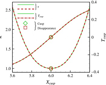
It is easy to show that for these velocity fields a cusp bifurcation appears in the vorticity field at $x=X_{cusp}$
if the amplitude of the perturbation is set to
$x=X_{cusp}$
if the amplitude of the perturbation is set to
 $$\begin{eqnarray}\displaystyle \unicode[STIX]{x1D716}=\sqrt{144(X_{cusp}-x_{0})^{4}+12(X_{cusp}-x_{0})^{2}+1}. & & \displaystyle\end{eqnarray}$$
The time when and the $y$
-position where this cusp bifurcation occurs are given by
$y$
-position where this cusp bifurcation occurs are given by
 $$\begin{eqnarray}\displaystyle T_{cusp}=\frac{1}{2\unicode[STIX]{x03C0}}\arctan \left(\frac{6(X_{cusp}-x_{0})}{1-12(X_{cusp}-x_{0})^{2}}\right) & & \displaystyle\end{eqnarray}$$
and
 $$\begin{eqnarray}\displaystyle Y_{cusp}=y_{0}+X_{cusp}-x_{0}, & & \displaystyle\end{eqnarray}$$
respectively. Equation (A 3) shows that for each value of $\unicode[STIX]{x1D716}>1$
a cusp bifurcation occurs at two values of
$\unicode[STIX]{x1D716}>1$
a cusp bifurcation occurs at two values of $X_{cusp}$
(symmetric about
$X_{cusp}$
(symmetric about $x_{0}$
); the cusp bifurcations disappear when they merge (at
$x_{0}$
); the cusp bifurcations disappear when they merge (at $(x_{0},y_{0})$
and at time
$(x_{0},y_{0})$
and at time $t=0$
) as
$t=0$
) as $\unicode[STIX]{x1D716}{\searrow}\unicode[STIX]{x1D716}_{K}=1$
. The velocity field therefore generates a vorticity field that has exactly the structure that we observe in our actual problem and therefore provides a good test case for the methodology.
$\unicode[STIX]{x1D716}{\searrow}\unicode[STIX]{x1D716}_{K}=1$
. The velocity field therefore generates a vorticity field that has exactly the structure that we observe in our actual problem and therefore provides a good test case for the methodology.
Figure 11 shows that our numerical method can accurately determine not only the position and time at which cusp bifurcations occur in the vorticity field, but also the value of the amplitude $\unicode[STIX]{x1D716}$
below which the cusp bifurcation disappears.
$\unicode[STIX]{x1D716}$
below which the cusp bifurcation disappears.


 Open access