


1. Introduction
Gravity currents or density currents are a horizontal intrusion of different density to an ambient fluid. Gravity currents are observed in many naturally occurring phenomena such as sandstorms (Parsons Reference Parsons2000), powder-snow avalanches (Turnbull & McElwaine Reference Turnbull and McElwaine2007) and bushfires (Dold, Zinoviev & Weber Reference Dold, Zinoviev and Weber2006). Comprehensive reviews of gravity currents in geophysical flows, laboratory experiments and numerical simulations are given by Simpson (Reference Simpson1982) and Meiburg, Radhakrishnan & Nasr-Azadani (Reference Meiburg, Radhakrishnan and Nasr-Azadani2015). We consider a body of heavy fluid initially at rest released into an ambient fluid at  $t=0$. The heavy fluid collapses and leads to an intrusion of fluid with a distinct head region. When the gravity current is formed, a well-defined shape is recognised and the flow develops into a highly turbulent head, quasi-steady body and shallower following tail (Cantero et al. Reference Cantero, Balachandar, García and Bock2008; Zordan, Schleiss & Franca Reference Zordan, Schleiss and Franca2018).
Experimental (Huppert & Simpson Reference Huppert and Simpson1980; Alahyari & Longmire Reference Alahyari and Longmire1996; Marino, Thomas & Linden Reference Marino, Thomas and Linden2005; Patterson, Simpson & Dalziel Reference Patterson, Simpson, Dalziel and van Heijst2006) and numerical (Blanchette et al. Reference Blanchette, Strauss, Meiburg, Kneller and Glinsky2005; Cantero, Balachandar & García Reference Cantero, Balachandar and García2007a; Cantero et al. Reference Cantero, Lee, Balachandar and García2007b, Reference Cantero, Balachandar, García and Bock2008) studies of planar and cylindrical gravity currents have found that propagation of a gravity current undergoes four main stages. As the heavy fluid is released, the gravity current undergoes an acceleration phase (zero to maximum), where the gravitational potential energy of the heavy fluid is converted into kinetic energy. A secondary acceleration is reported by Zhu et al. (Reference Zhu, Zgheib, Balachandar and Ooi2017) and Ooi, Zgheib & Balachandar (Reference Ooi, Zgheib and Balachandar2015) who conducted numerical simulations of a circular gravity current on a uniform slope. The secondary acceleration phase is due to the rearrangement and redistribution of the heavy fluid in the current which increases the buoyancy at the downstream end of the current. After the front velocity reaches its maximum, the acceleration phase is followed by the slumping phase, where the front height and speed remain constant. In this phase, the axisymmetric (cylindrical) current head comprises a coherent counter-clockwise (or clockwise, depending on the azimuthal direction being observed) rotating vortex ring. This ring is formed due to the roll-up of the interface shear layer between the heavy and ambient fluids. The effects of stretching and tilting of the vortex ring on the dynamics of axisymmetric (cylindrical) currents have been explored by Patterson et al. (Reference Patterson, Simpson, Dalziel and van Heijst2006) and Cantero et al. (Reference Cantero, Balachandar and García2007a). Next, the gravity current transitions into the self-similar inertial phase in which the buoyancy force is balanced by the inertial force. The gravity current eventually reaches the viscous phase wherein the viscous force dominates the buoyancy force. In the inertial and viscous phases, it has been reported that the front velocity of the gravity current decays as a power law (Fay Reference Fay1969; Hoult Reference Hoult1972; Cantero et al. Reference Cantero, Lee, Balachandar and García2007b, Reference Cantero, Balachandar, García and Bock2008).
Stratification of the ambient fluid can greatly affect the propagation and dynamics of the gravity current. Additionally, the presence of stratification leads to the generation of internal waves. The specific layer through which the gravity current propagates depends on the relative strength of the current ( $\rho _c^*-\rho _0^*$) and the ambient stratification ( $\rho _b^*-\rho _0^*$) (Maxworthy et al. Reference Maxworthy, Leilich, Simpson and Meiburg2002; Dai, Huang & Hsieh Reference Dai, Huang and Hsieh2021). In stratified environments, intrusive gravity currents can occur when the density of the heavy fluid matches the density at an intermediate level (see Flynn & Sutherland Reference Flynn and Sutherland2004; Ungarish Reference Ungarish2005b; la Forgia et al. Reference la Forgia, Ottolenghi, Adduce and Falcini2020; Ottolenghi et al. Reference Ottolenghi, Adduce, Roman and la Forgia2020). Conversely, gravity currents propagate along the bottom boundary when the density of the heavy fluid is equal to or greater than the density at the bottom of the stratified ambient (Maxworthy et al. Reference Maxworthy, Leilich, Simpson and Meiburg2002; Ungarish Reference Ungarish2005a; Birman, Meiburg & Ungarish Reference Birman, Meiburg and Ungarish2007b; White & Helfrich Reference White and Helfrich2008). In this paper, we will only consider the case where the stratification of the ambient fluid is linear for a horizontal domain of uniform depth and the current is denser than the ambient. We will also assume that the release is of full-depth.
Various experimental and numerical studies have been carried out to investigate the propagation of a gravity current into a stratified ambient fluid. Mitsudera & Baines (Reference Mitsudera and Baines1992) conducted an experimental study of a downslope gravity current flow in a continuously stratified ambient fluid to model the Bass Strait outflow. An experimental and numerical study was conducted by Maxworthy et al. (Reference Maxworthy, Leilich, Simpson and Meiburg2002) to investigate the relationship between the internal Froude number of the gravity current and stratification  $S$ in the ambient and
 \begin{equation} S=\frac{\rho_b^*-\rho_0^*}{\rho_c^*-\rho_0^*}. \end{equation}
The flow regime of the gravity current flow is determined by the Froude number based on the buoyancy frequency which is a dimensionless parameter defined as the ratio of the inertial forces relative to the gravitational forces, i.e.  $Fr=u^*_{f,mean}/N^*H^*$, where $u^*_{f,mean}$ is the mean front velocity in the slumping phase, $(N^*)^2 =(g^*/\rho _0^*)(-{\rm d}\rho ^*/{\rm d}z^*)= g^*(\rho _b^* - \rho _0^*)/\rho _0^* H^*$ is the buoyancy frequency, $g^*$ is the gravitational acceleration, $\rho ^*$ is the dimensional fluid density, $z^*$ is the vertical coordinate and $H^*$ is the depth of the domain. Note that in this manuscript, variables with asterisks ( $*$) denote dimensional variables. In the subcritical regime ( $Fr<1/{\rm \pi}$), the gravity current propagates slower than the maximum speed of the linear internal gravity wave ( $N^*H^*/{\rm \pi}$) and minimal (or no) vortices are observed behind the gravity current head, whereas in the supercritical regime ( $Fr>1/{\rm \pi}$), the gravity current flow becomes turbulent and strong Kelvin–Helmholtz (K–H) billows can be observed behind the head.
A similar study was conducted by Ungarish & Huppert (Reference Ungarish and Huppert2002) using the shallow-water approximation and found excellent agreement with the experimental results presented by Maxworthy et al. (Reference Maxworthy, Leilich, Simpson and Meiburg2002). It is worth noting that the propagation speed of the gravity current is reduced by the stratified ambient compared with the homogeneous ambient (where the density of the ambient fluid is constant throughout the domain). A similar phenomenon was previously observed by Lam et al. (Reference Lam, Chan, Hasini and Ooi2018a,Reference Lam, Chan, Hasini and Ooib), Lam, Chan & Ooi (Reference Lam, Chan and Ooi2022b) who conducted direct numerical simulations (DNSs) of a two-dimensional gravity current flow in a stratified ambient to investigate the effects of the initial aspect ratio and the strength of stratification on the dynamics of the gravity current flow. Lam et al. (Reference Lam, Chan, Hasini and Ooi2018b) reported that in the subcritical regime, the gravity current contains minimal vortices whereas, in the supercritical regime, the gravity current becomes turbulent and strong vortices are observed in the gravity current head.
Planar release gravity currents in stratified (Maxworthy et al. Reference Maxworthy, Leilich, Simpson and Meiburg2002; Ungarish & Huppert Reference Ungarish and Huppert2002; Birman et al. Reference Birman, Meiburg and Ungarish2007b; Longo et al. Reference Longo, Ungarish, Di Federico, Chiapponi and Addona2016; Chiapponi et al. Reference Chiapponi, Ungarish, Longo, Di Federico and Addona2018; Lam et al. Reference Lam, Chan, Hasini and Ooi2018b; la Forgia et al. Reference la Forgia, Ottolenghi, Adduce and Falcini2020; Ottolenghi et al. Reference Ottolenghi, Adduce, Roman and la Forgia2020; Dai et al. Reference Dai, Huang and Hsieh2021; Zahtila et al. Reference Zahtila, Lam, Chan, Sutherland, Moinuddin, Dai, Skvortsov, Manasseh and Ooi2024), and unstratified ambients (Rottman & Simpson Reference Rottman and Simpson1983; Shin, Dalziel & Linden Reference Shin, Dalziel and Linden2004; La Rocca et al. Reference La Rocca, Adduce, Sciortino and Pinzon2008; Dai Reference Dai2015; Pelmard, Norris & Friedrich Reference Pelmard, Norris and Friedrich2018; Dai & Huang Reference Dai and Huang2020; De Falco, Adduce & Maggi Reference De Falco, Adduce and Maggi2021; Maggi, Adduce & Negretti Reference Maggi, Adduce and Negretti2022, Reference Maggi, Adduce and Negretti2023a; Maggi et al. Reference Maggi, Negretti, Hopfinger and Adduce2023b), as well as cylindrical release gravity currents in unstratified environment have been widely studied experimentally and numerically (Cantero et al. Reference Cantero, Balachandar and García2007a,Reference Cantero, Lee, Balachandar and Garcíab; Zgheib, Bonometti & Balachandar Reference Zgheib, Bonometti and Balachandar2014, Reference Zgheib, Bonometti and Balachandar2015a; Dai & Huang Reference Dai and Huang2016). However, experimental and numerical studies on stratified gravity currents with the cylindrical release are limited, and therefore we are interested in cylindrical gravity currents propagating into a linearly stratified ambient.
Birman et al. (Reference Birman, Meiburg and Ungarish2007b) examined the model developed by Ungarish (Reference Ungarish2006) (where the hydraulic theory from Benjamin (Reference Benjamin1968) was generalized to a linearly stratified ambient) on the dependency of the front velocity on the stratification strength ( $S$). The model was found to work well for weak stratification ( $S \leq 0.5$). Ungarish & Huppert (Reference Ungarish and Huppert2006) analysed the exchange of energy of gravity currents propagating into an unstratified and linearly stratified ambient with the shallow-water model and two-dimensional (2-D) Navier–Stokes simulations. Good agreement between the shallow-water model and the 2-D simulations was obtained up to the end of the inertial phase as the viscous effects were not included in the shallow-water model. Ungarish & Huppert (Reference Ungarish and Huppert2008) then analysed the energy balances of an axisymmetric gravity current in the homogeneous ambient and linearly stratified ambient using the shallow-water model and Navier–Stokes finite difference simulations within a two-dimensional geometry. A fair agreement on the energy changes of the current was also obtained between these two approaches. Similar observations reported by Ungarish & Huppert (Reference Ungarish and Huppert2006) were obtained in this study too where the stratification in the ambient enhanced the accumulation of potential energy and reduced the energy dissipation in the system.
Previous literature has explored the dynamics of gravity currents in unstratified ambients with varying aspect ratios and depth ratios of heavy fluid on a horizontal plane (or on a uniform slope). The front location, front velocity and theoretical or empirical models to predict the front velocity during the slumping, inertial and viscous phases have been determined for both planar and cylindrical currents in an unstratified ambient. Some studies have also investigated the effects of stratification on planar currents, but to our knowledge, no studies have investigated fully three-dimensional (3-D) cylindrical gravity currents in a stratified ambient. Such studies are important because cylindrical currents behave differently from planar currents. For example, the spreading rate of a planar current increases linearly, while that of a cylindrical current increases quadratically. Furthermore, the propagation of a current can be affected by a stratified ambient, as reported by Birman et al. (Reference Birman, Meiburg and Ungarish2007b), Lam et al. (Reference Lam, Chan, Hasini and Ooi2018a,Reference Lam, Chan, Hasini and Ooib, Reference Lam, Chan, Hasini and Ooi2022a,Reference Lam, Chan and Ooib) and Dai et al. (Reference Dai, Huang and Hsieh2021).
This study aims to investigate the effects of the strength of the stratification,  $S$, and Reynolds number, $Re$, on the dynamics of the cylindrical release gravity current flow on the horizontal plane. In this work, we present the results from fully 3-D DNSs of cylindrical gravity currents propagating in a linearly stratified ambient with varying stratification at moderate Reynolds numbers. A detailed study on predicting the front velocity in the different phases as well as the scaling for the front velocity for both unstratified and stratified cases in the slumping phase is explored. Analysis of the density contours is used to compare the flow structures at different Reynolds numbers and stratification strengths. The three-dimensional structure of the advancing front is compared between the unstratified and stratified cases. The paper is structured as follows. Section 2 describes the numerical procedure including the governing equations, initial and boundary conditions, and the formulation of the problem. In § 3, the theoretical and empirical models in predicting the front velocity in the different phases and the impact of stratification on the front velocity in the slumping phase will be analysed. In § 4, we present our simulation results as well as a discussion of these results. Finally, conclusions are drawn in § 5.
2. Computational set-up
The 3-D, cylindrical release gravity currents in a stratified ambient have been simulated using Nek5000, a spectral element, incompressible flow solver (Fischer, Lottes & Kerkemeier Reference Fischer, Lottes and Kerkemeier2008). Here, we adopt the Boussinesq approximation where the density difference between two fluids is sufficiently small (less than  $5\,\%$) (Turner Reference Turner1979) to neglect the influence of density differences in the inertial and diffusion terms, and retains only in the buoyancy term (Dai et al. Reference Dai, Huang and Hsieh2021; Cao, Philip & Ooi Reference Cao, Philip and Ooi2022). The non-dimensional governing equations employed in the study take the form
 \begin{gather} \boldsymbol{\nabla} \boldsymbol{{\cdot}} \boldsymbol{u}=0, \end{gather}
 \begin{gather}\frac{{\rm D}\boldsymbol{u}}{{\rm D}t}={-}\rho \boldsymbol{\hat{z}} - \boldsymbol{\nabla} p + \frac{1}{Re} \nabla^2 \boldsymbol{u}, \end{gather}
 \begin{gather}\frac{\partial \rho}{\partial t} + \boldsymbol{\nabla} \boldsymbol{{\cdot}} (\rho \boldsymbol{u}) = \frac{1}{Re Sc}\nabla^2\rho, \end{gather}
where  $\rho$ is the density of the fluid, $\boldsymbol {u}=[u,v,w]$ is the velocity for 3-D flow, $p$ is pressure and $\boldsymbol {\hat {z}}$ is the unit vector in the positive $z$-direction. The dimensionless density, $\rho$, is defined as
 \begin{equation} \rho=\frac{\rho^* - \rho^*_0}{\rho^*_c - \rho^*_0}, \end{equation}
where the symbols  $\rho ^*$, $\rho ^*_0$ and $\rho ^*_c$ with asterisks are the dimensional density of the local, top of the domain and heavy fluid, respectively. The value of $\rho$ is bounded between 0 and 1. In the ambient fluid, the dimensionless density in the ambient $\rho _a$ varies linearly with depth $z$ from $\rho _a=\rho _b=S$ at the bottom $(z=0)$ to $\rho _a=\rho _0=0$ at the top $(z=1)$ and
 \begin{equation} \rho_{a}=\rho_{a}(z,t=0)=S(1-z). \end{equation}
The Schmidt number is  $Sc=\nu ^*$/ $\kappa ^*$ (where $\nu ^*$ is the kinematic viscosity and $\kappa ^*$ is the molecular diffusivity). Although saline, which is typically used in experiments, has $Sc=700$, it is found that when $Sc$ is of the order of 1 or larger, there is a weak scaling with the dynamics of the gravity current that does not significantly affect the bulk flow results (Härtel, Meiburg & Necker Reference Härtel, Meiburg and Necker2000; Necker et al. Reference Necker, Härtel, Kleiser and Meiburg2005; Cantero et al. Reference Cantero, Lee, Balachandar and García2007b; Bonometti & Balachandar Reference Bonometti and Balachandar2008; Dai Reference Dai2015). Therefore, $Sc=1$ is used in all simulations in the study.
The height of the domain  $H^*$ is taken as the length scale. The velocity scale, $U^*$, time scale, $T^*$, and the Reynolds number, $Re$, are defined as
 \begin{equation} U^*=\sqrt{g^\prime H^*}, \quad T^*=\frac{H^*}{U^*}, \quad Re=\frac{U^*H^*}{\nu^*}, \end{equation}
where  $g^\prime =g^*(\rho _c^*-\rho _0^*)/\rho _0^*$ is the reduced gravity and $g^*$ is the gravitational acceleration acting in the negative $z$ direction.
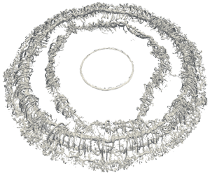
Figure 1 shows the initial configuration of a full-depth cylindrical-release gravity current in a linearly stratified ambient with  $S=0.5$. The horizontal directions are represented by $x$ and $y$, while the wall-normal direction is represented by $z$. The computational domain is a square prism with $L_x = L_y = 30$ ( $L_x = L_y = 20$ for the cases with higher Reynolds number to reduce computational cost). A cylindrical lock contained heavy fluid with a density of $\rho _c$ has a height $H=1$ and unit radius ( $r_0$) is contained at the centre of the computational domain. The density of the ambient ( $\rho _a$) is increased linearly from the top ( $\rho _0)$ to the bottom ( $\rho _b$). A no-slip boundary condition is employed at the bottom ( $z = 0$) of the domain and a slip, impermeable symmetry boundary condition is applied at the top of the domain ( $z=1$) and vertical side walls ( $x=[-L_x/2,L_x/2]$ and $y=[-L_y/2,L_y/2]$).

Figure 1. Sketch of the computational domain for the 3-D simulation. he horizontal directions are represented by  $x$ and $y$, while the wall-normal direction is represented by $z$. The cylindrical region of heavy fluid located in the centre of the domain has a density of $\rho _c$. The heavy and ambient fluid has the same height as the height of the domain $H$. The density of the ambient $\rho _a(z)$ increases linearly from the top $\rho _0$ to the bottom boundary $\rho _b$ as indicated by the lighter grey shading and the $\rho _a(z)$ shown on the top left wall.
In this study, we have systematically investigated the effects of the stratification strength on the dynamics of the cylindrical gravity current. Four stratification strength of  $S = 0$, 0.2, 0.5 and 0.8 are considered and simulated at Reynolds numbers of $Re = 3450$ and 10 000. Here, seventh-order polynomial spectral elements are used in this study to reduce numerical error in the simulation. The number of spectral elements employed for the simulations at low and high $Re$ are $N_x \times N_y \times N_z = 190 \times 190 \times 15$ and $270 \times 270 \times 20$, respectively. The grid distribution within the spectral element follows the Gauss–Legendre–Lobatto (GLL) grid spacing. This total number of unique grid points is $1.9\times 10^8$ and $5\times 10^8$ grid points. Grid stretching (geometrical progression with power coefficient) is applied along the wall-normal direction ( $z$) where the grid size at the bottom part is denser than the top. The computational grid has a grid spacing of $0.0033 \leq \Delta x = \Delta y \leq 0.0332$ for $Re=3450$ and $0.0021 \leq \Delta x = \Delta y \leq 0.0165$ for $Re=10\,000$. The grid spacing to Kolmogorov scale ratio, $\Delta l/\eta$ (where $\Delta l = (\Delta x \Delta y \Delta z)^{1/3}$ and $\eta$ is the local dissipation) is calculated at different instantaneous time and is always less than 10. This is more conservative than the $\Delta l/\eta \approx 16$ recommended by Lu et al. (Reference Lu, Aljubaili, Zahtila, Chan and Ooi2023) and Zahtila et al. (Reference Zahtila, Lu, Chan and Ooi2023), who studied the grid convergence characteristics of spectral element solvers. Therefore, we have ensured that our grid resolution is sufficient to resolve all of the turbulent length scales and also meet the requirement of $\Delta x = \Delta y \approx (ReSc)^{-1/2}$, where $Sc = 1$ (Härtel et al. Reference Härtel, Meiburg and Necker2000; Birman, Martin & Meiburg Reference Birman, Martin and Meiburg2005; Dai Reference Dai2015). A variable time step is used to ensure that the Courant number is always less than 0.5 and the simulation is run for a total time of $T=60$.
3. Theoretical predictions of front velocity
This section describes the theoretical and empirical models for predicting the front velocity of a cylindrical gravity current during the slumping, inertial and viscous phases as it propagates into an unstratified ambient. In the following sections of this paper, we will discuss the effect of stratification on the prediction of the front velocity during the slumping phase.
3.1. Slumping phase
Several theoretical and empirical models have been proposed to predict the front velocity during the slumping phase. First, Benjamin (Reference Benjamin1968) derived the Froude number of the front using hydraulic theory. The expression of the current speed in terms of Froude number based on the depth  $H^*$ of the ambient fluid is expressed as
 \begin{equation} Fr_B = \frac{u_f^*}{\sqrt{g^\prime H^*}} = \sqrt{\tilde{h}(2-\tilde{h}) \frac{(1-\tilde{h})}{(1+\tilde{h})}}, \end{equation}
where  $u_f$ is the constant front velocity and $\tilde {h}=h^*/H^*$ is the dimensionless current height. In the limit of $\tilde {h} \rightarrow 0.5$, $Fr_B = 0.5$. Shin et al. (Reference Shin, Dalziel and Linden2004) extended Benjamin's theory by taking into consideration the exchange between the advancing front of the gravity current and the backward disturbance. Both full-depth and partial-depth releases are taken into account in the study, and the speed of the current has the expression of
 \begin{equation} Fr_S = \tfrac{1}{2}\sqrt{\tilde{D}(2-\tilde{D})}, \end{equation}
where  $\tilde {D}=D^*/H^*$ is the dimensionless initial depth of the heavy fluid. In the limit of full-depth release, $\tilde {D}=1$, the above expression yields the same results as (3.1).
Huppert & Simpson (Reference Huppert and Simpson1980), however, reported an empirical expression for the Froude number at the gravity current head based on the experimental measurement as
 \begin{equation} Fr_{HS} =\begin{cases} \frac{1}{2}\tilde{h}_{HS}^{1/6} & (0.075 \leq \tilde{h}_{HS} \leq 1),\\ 1.19\tilde{h}_{HS}^{1/2} & (0 \leq \tilde{h}_{HS} \leq 0.075), \end{cases} \end{equation}
where  $\tilde {h}_{HS}$ is the dimensionless depth of the current just behind the head. In the limit of $\tilde {h}_{HS} \rightarrow 0.5$, the value of $Fr_{HS} \approx 0.45$ is slightly lower than the value of 0.5 predicted by Benjamin (Reference Benjamin1968) and Shin et al. (Reference Shin, Dalziel and Linden2004). Here the subscript $B$,
$B$,  $S$ and $HS$ denotes Benjamin (Reference Benjamin1968), Shin et al. (Reference Shin, Dalziel and Linden2004) and Huppert & Simpson (Reference Huppert and Simpson1980). Previous studies (Bonnecaze et al. Reference Bonnecaze, Hallworth, Huppert and Lister1995; Ungarish & Huppert Reference Ungarish and Huppert1998; Hallworth, Huppert & Ungarish Reference Hallworth, Huppert and Ungarish2001) that study axisymmetric currents have adopted the empirical Froude number reported by Huppert & Simpson (Reference Huppert and Simpson1980) (see (3.3)) in their studies and the results are consistent with the results obtained using different methods such as numerical simulation, experimental measurement and shallow-water approximations. Cantero et al. (Reference Cantero, Lee, Balachandar and García2007b), however, reported that the three-dimensionality of the current does not have a strong influence on the speed of the current during the slumping phase but becomes important during the inertial and viscous phases. Numerical results from Cantero et al. (Reference Cantero, Lee, Balachandar and García2007b) show a good agreement with the experimental data from Hallworth et al. (Reference Hallworth, Huppert and Ungarish2001) when compared with the planar theory. Therefore, the slumping velocity from planar theory will be used for comparison with current simulation results.
The theoretical and empirical models for the mean front velocity in the slumping phase for unstratified gravity currents overestimate the front velocity of gravity currents in a stratified ambient. Ungarish & Huppert (Reference Ungarish and Huppert2002) claimed that the mean front velocity in the slumping phase in the Froude condition reported by Huppert & Simpson (Reference Huppert and Simpson1980) (see (3.3)) is a function of  $\tilde {h}_{HS}$ with stratification strength ( $S$) and height of channel ( $H$) as parameters. The proposed mean front velocity in the slumping phase for the gravity current in a stratified ambient is
 \begin{equation} Fr_{UH}(\tilde{h},S) = Fr_\xi(\tilde{h})(1-S+\tfrac{1}{2}\tilde{h}S)^{1/2}, \end{equation}
where  $Fr_\xi (\tilde {h})$ is the Froude number and the subscript $\xi$ denotes $B,HS$ and $C$ (corresponding to Benjamin Reference Benjamin1968; Huppert & Simpson Reference Huppert and Simpson1980 and Cantero et al. Reference Cantero, Lee, Balachandar and García2007b), respectively.
Ungarish (Reference Ungarish2006) adapts Long's model (Long Reference Long1953, Reference Long1955; Baines Reference Baines1995) and the Froude number is defined as
 \begin{equation} Fr_U(\tilde{h},S)=Fr_\xi(\tilde{h})(1-\tfrac{2}{3}S)^{1/2}. \end{equation}
Here, the subscript  $UH$ and $U$ denotes Ungarish & Huppert (Reference Ungarish and Huppert2002) and Ungarish (Reference Ungarish2006). Ungarish (Reference Ungarish2006) concludes that $Fr$ rescaling is useful for the case with weak stratification but significantly underestimates $Fr$ when $S/\tilde {h}>5$ (larger $S$ and/or small $\tilde {h}$). Birman et al. (Reference Birman, Meiburg and Ungarish2007b) conducted two-dimensional simulations of planar gravity currents propagating in a stratified ambient with initial fractional depth $\tilde {h}_0 = 0.2$, 0.5 and 1 with $S$ ranging from 0.2 to 0.9 at $Re=4000$. The front velocity of the current in the slumping phase as a function of $S$ was compared with the theoretical model by Ungarish (Reference Ungarish2006). Birman et al. (Reference Birman, Meiburg and Ungarish2007b) reported that the model is found to predict well in determining the Froude number with weak stratification. For strong stratification ( $S>0.5$), multiple solutions exist and the solutions deviate from the first theoretical solution but agree closely to the second or third theoretical solutions.
3.2. Inertial phase
After the slumping phase, the gravity current in an unstratified ambient transitions into the first self-similar regime, the inertial phase. Here, the reflected backward propagating wave catches the front with a speed slightly greater than the speed of the front (Rottman & Simpson Reference Rottman and Simpson1983). During the inertial phase, the buoyancy force is balanced by the inertial force and the front velocity of the current decreases as a power law,  $t^{-1/2}$ for the cylindrical current (Cantero et al. Reference Cantero, Lee, Balachandar and García2007b) in the inertial phase. Models for gravity currents in the inertial phase have been proposed by Fay (Reference Fay1969), Fannelop & Waldman (Reference Fannelop and Waldman1972), Hoult (Reference Hoult1972), Huppert & Simpson (Reference Huppert and Simpson1980) and Rottman & Simpson (Reference Rottman and Simpson1983). The asymptotic behaviour of the cylindrical current in the inertial phase is
 \begin{equation} r_f = {\rm \pi}^{1/4}\xi_{ip} h_0^{1/4}(r_0t)^{1/2},\quad u_f = \tfrac{1}{2}\xi_{ip} h_0^{1/4}r_0^{1/2}t^{{-}1/2}, \end{equation}
where  $r_f$ is the radial front location of the cylindrical current, $\xi _{ip}$ is a constant for the cylindrical current and the subscript $ip$ denotes the inertial phase. The initial height and radius of the lock are $h_0$ and $r_0$. Hoult (Reference Hoult1972) and Huppert & Simpson (Reference Huppert and Simpson1980) proposed $\xi _{ip}= 1.3$ and 1.16, respectively. Cantero et al. (Reference Cantero, Lee, Balachandar and García2007b) investigates the transition between the different phases on 3-D cylindrical gravity currents at $Re= 895$, 3450 and 8950. A range of experimental data was used to revisit the scaling during the phases of spreading for cylindrical release gravity current. The best-fit value of the constants $\xi _{ip}$ was found to be 1.23 for the cylindrical current.
3.3. Viscous phase
Finally, the gravity current reaches the second self-similar regime, the viscous phase when the viscous force becomes significant compared with the buoyancy force. Fay (Reference Fay1969) and Hoult (Reference Hoult1972) predict the self-similar solution for the cylindrical current using a boundary layer approximation
 \begin{equation} r_f = \xi_{vp, Ht}h_0^{1/3}r_0^{2/3}Re^{1/12}t^{1/4},\quad u_f = \tfrac{1}{4}\xi_{vp, Ht}h_0^{1/3}r_0^{2/3}Re^{1/12}t^{{-}3/4}, \end{equation}
where the subscript  $vp$ denotes the viscous phase. The solution from Hoult (Reference Hoult1972) has a constant value of $\xi _{vp, Ht}=1.38$. Huppert (Reference Huppert1982) revised the analysis by considering the viscous effect over a rigid horizontal surface. The self-similar solutions obtained for the viscous phase differ from those presented in (3.7) and are expressed as
 \begin{equation} r_f = \xi_{vp, Hp}h_0^{3/8}r_0^{3/4}Re^{1/8}t^{1/8},\quad u_f = \tfrac{1}{8}\xi_{vp, Hp}h_0^{3/8}r_0^{3/4}Re^{1/8}t^{{-}7/8}, \end{equation}
where  $\xi _{vp, Hp}=1.197$. Here the subscript $Ht$ and $Hp$ denotes Hoult (Reference Hoult1972) and Huppert (Reference Huppert1982), respectively.
4. Results and discussion
4.1. Equivalent height of the gravity current
The equivalent height, defined as the azimuthally averaged integrated height of the current in the wall-normal direction ( $z$), is defined by
 \begin{equation} \bar{h}(r,t) =\frac{1}{2{\rm \pi}}\int_{0}^{H}\int_{0}^{2{\rm \pi}}\rho(r,\theta,z,t)\, {\rm d}\theta \,{\rm d}z - \int_{0}^{H}\rho_a(z)\,{\rm d}z. \end{equation}
Note that in this definition of equivalent height, the total mass of the gravity current is  $1/R\times \int ^R_0 \bar {h}r\, {\rm d}r$, where $R$ is the radius of the domain. The equivalent height provides a good indication of the distribution of mass in the streamwise direction and the shape of the gravity current (Shin et al. Reference Shin, Dalziel and Linden2004; Marino et al. Reference Marino, Thomas and Linden2005; Birman et al. Reference Birman, Battandier, Meiburg and Linden2007a; Cantero et al. Reference Cantero, Lee, Balachandar and García2007b; Dai Reference Dai2015). However, when stratification is introduced to the ambient fluid, it changes the equivalent height ( $\bar {h}$) by an amount proportional to the stratification strength $S$. This is reflected in the second term of (4.1), which is equal to $S/2$ and is zero in an unstratified case where $\rho _a=0$. It should be noted that as the strength of stratification increases, the interface between the intrusion and the ambient becomes smoother and less distinguishable (Sutherland et al. Reference Sutherland, Chan, Ooi, Chan and Wai Kit2022). Before we examine the propagation in detail, we analyse the density contours and equivalent height of the gravity current with different $S$ at $Re=3450$ and 10 000 to characterise the flow in the slumping and inertial phases, the two most persistent and interesting phases.
Figure 2 shows the time evolution of the azimuthally averaged density contour of the gravity current at  $Re= 3450$ for $S=0$, 0.2, 0.5 and 0.8, respectively. The equivalent height ( $\bar {h}$) of the current is plotted on top of the density contour ( $\rho =0.015$). In the slumping phase, strong K–H vortices are formed behind the head of the gravity current. The rolled-up vortices entrain ambient fluid and mix with it, and these structures are reflected in the local maximum of the equivalent height. The height of the current in the head region does not differ significantly during the slumping phase for $S\leq 0.5$. Weaker vortices are formed in the case with strong stratification ( $S=0.8$) and the current head results in a smaller head size than the other cases. Also, we can observe the head is slightly lifted from the bottom wall in all cases and in all phases due to the no-slip condition, and a layer of ambient fluid is entering and mixing with the head. A similar observation is also reported by Cantero et al. (Reference Cantero, Balachandar and García2007a). At $t=10.4$, the current with $S=0$ has transitioned into the inertial phase and the K–H billow has mixed with the head. A similar observation is observed for $S=0.2$ and 0.5 in the inertial phase. At a similar time $t=10$ for $S=0.8$, the K–H billow is still presented behind the current and this shows that stratification delayed the transition of the current.

Figure 2. Azimuthal-averaged density contour of the gravity current ( $\rho =0.015$) with $S=$ (a) 0, (b) 0.2, (c) 0.5 and (d) 0.8 at $Re= 3450$. The red box shows the head is lifted from the bottom wall. The solid black line shows the equivalent height of the gravity current ( $\bar {h}$). SP, slumping phase and IP, inertial phase.
4.2. Front location and front velocity
The front location of the gravity current is typically defined as the location where the equivalent height,  $\bar {h}$, is smaller than an arbitrarily small threshold $\delta$ (Cantero et al. Reference Cantero, Lee, Balachandar and García2007b; Dai Reference Dai2015; Zhu et al. Reference Zhu, Zgheib, Balachandar and Ooi2017; Chan, Lam & Ooi Reference Chan, Lam and Ooi2018). However, for a gravity current in a stratified ambient, this method leads to an overestimation in the front location due to a displaced bottom layer. Therefore, the gradient of the equivalent height method is used as it is more robust for flows with strong stratification. This method is explained in more detail and its accuracy is compared with a few different methods in Appendix A.
Figure 3(a) shows the plot of the front location for the cases with stratification strength ranging from 0 to 0.8 at  $Re= 3450$ (solid lines) and 10 000 (open circles). The front location of the gravity current is plotted until the front has mixed with the ambient fluid and is not detectable. Increasing the linear stratification strength leads to a reduction in the distance travelled by the front of the gravity current at the end of the slumping phase. At $t=16$, which is approximately when the gravity current for the case $S=0.8$ at $Re=3450$ has dissipated and there is no appreciable or discernible gravity current flow any more, the gravity current propagated for approximately 3.8 lock radii ( $r_f \approx 4.8$), which is approximately $22\,\%$ smaller than the distance travelled in the unstratified ambient case ( $S=0$), where the current travelled approximately 4.6 lock radii ( $r_f \approx 5.6$). Similarly, in the high- $Re$ case, for $S=0.8$, the distance travelled was approximately 4.2 lock radii ( $r_f=5.2$), representing a reduction of approximately $17\,\%$ compared to the unstratified case, where the travel distance was 4.9 lock radii ( $r_f \approx 5.9$) at $t=17$.

Figure 3. Plot of (a) front location, (b) front location with time offset ( $t_0$) and (c) front velocity against time for stratified cylindrical release gravity current with different stratification strength ranging from $S= 0$ to 0.8 at $Re= 3450$ (—) and 10 000 ( $\circ$). The stratification is represented with a different colour where red, $S= 0$; green, $S= 0.2$; blue, $S= 0.5$ and cyan, $S= 0.8$. The predicted front location using the theoretical models for $S=0$ at $Re=10\,000$ are included in the plot where ( $*$), inertial phase in (3.6); ( $\vartriangle$), viscous phase by Hoult (Reference Hoult1972) in (3.7); ( $\triangledown$), viscous phase by Huppert (Reference Huppert1982) in (3.8) with $Re=10\,000$, $h_0=1$ and $r_0=1$. The dashed line shows the maximum speed of the linear internal gravity wave, $N^*H^*/{\rm \pi}$ for different stratification strengths: green, $S= 0.2$; blue, $S= 0.5$ and cyan, $S= 0.8$.
The predicted front location for  $S=0$ using the scaling in the inertial and viscous phase is also included in figure 3(b) and is represented with different line styles. It is important to note that the physical simulation time will not correspond to the virtual time origin (Samasiri & Woods Reference Samasiri and Woods2015; Sher & Woods Reference Sher and Woods2015). Therefore, we have estimated a value of the virtual origin in time, $t_0$, for all the cases in the inertial phase using the method proposed by Sher & Woods (Reference Sher and Woods2015) and Samasiri & Woods (Reference Samasiri and Woods2015). Figures 3(b) and 4 show the front velocity profiles collapse in the inertial phase irrespective of the Reynolds number and stratification strength, at least for the range of $Re$ and $S$ considered in this study. The front location of the gravity current for both low and high $Re$ with $0\leq S<0.5$ cases follows the inertial phase scaling of $t^{1/2}$ (represented by $*$) reported by Huppert & Simpson (Reference Huppert and Simpson1980) (defined in (3.6)). For the strongly stratified cases ( $S=0.8$), the propagation of the current becomes negligible during the slumping phase due to the insufficient density difference between the current and the ambient at the bottom wall. As a result, there is no longer any gravity current flow.

Figure 4. Plot of the front velocity against time for stratified cylindrical release gravity current with different stratification strengths ranging from  $S= 0$ to 0.8 at $Re=$ (a) 3450 and (b) 10 000. The stratification is represented with a different colour where red solid line (circle) $,S=0$; green solid line (circle), $S= 0.2$; blue solid line (circle), $S= 0.5$ and cyan solid line (circle), $S= 0.8$. The theoretical model for $S=0$, (black solid line), slumping phase; ( $\cdots \cdots$), inertial phase; (– – –), viscous phase by Hoult (Reference Hoult1972) in (3.7); (- $\cdot$- $\cdot$), viscous phase by Huppert (Reference Huppert1982) in (3.8).
The proposed scalings in the viscous phase by Hoult (Reference Hoult1972) and Huppert (Reference Huppert1982) (represented by the  $\vartriangle$ and $\triangledown$) underestimate the front locations of the gravity current. However, the trend of the scalings shows a good agreement with the simulation result for both low- and high- $Re$ cases within the range of $0\leq S<0.8$. The front location for $Re$ with $S=0$ in the viscous phase evolves at approximately $t^{0.28}$. This is closer to the viscous scaling $t^{1/4}$ in (3.7), and it is larger than the viscous scaling $t^{1/8}$ in (3.8) by a factor of 2. For the stratified cases, the propagation of the current becomes negligible in the early stage of the viscous phase (or does not transition into the viscous phase). Therefore, no observation is made for those cases. Cantero et al. (Reference Cantero, Lee, Balachandar and García2007b) optimised the prefactors of the scalings law and reported the empirical best-fit value of $\xi _{ip}=1.23$, $\xi _{vp, Ht}=2.6$ and $\xi _{vp, Hp}=4.64$ from the front velocity plot. With a slight modification of the prefactors, we found $\xi _{ip}=1.23$, $\xi _{vp, Ht}=2.96$ and $\xi _{vp, Hp}=6.56$ provides a fair agreement with our simulation results. However, these prefactors are not suitable for scaling laws in predicting the front location of the gravity current.
The front velocity of the gravity current is determined by applying a moving-average filter with filter width of  $\Delta t=1$ to the front location and then differentiating the filtered front location with respect to the time ( $u_f = {\rm d}r_f/{\rm d}t$). The plot of the front velocity against time for all cases is presented in figure 3(c). In the cylindrical release gravity current, similar to a planar release, we observe the propagation of gravity current undergoes four main flow phases as reported by Blanchette et al. (Reference Blanchette, Strauss, Meiburg, Kneller and Glinsky2005), Cantero et al. (Reference Cantero, Balachandar and García2007a,Reference Cantero, Lee, Balachandar and Garcíab, Reference Cantero, Balachandar, García and Bock2008) and these phases are discussed in the following.
The first phase is the initial acceleration where the front velocity accelerates from 0 to a maximum value. The maximum front velocity increases with  $Re$ but decreases as $S$ increases. As $S$ increases ( $S = 0, 0.2, 0.5, 0.8$), the peak value of the front velocity decreases from 0.563 to 0.512, 0.485 and 0.414 at $Re=3450$ and from 0.594 to 0.545, 0.514 and 0.437 at $Re=10\,000$. It is also noted that the duration of the acceleration phase is also extended with increasing $S$ with the gravity current taking a longer time to reach the maximum front velocity. Comparing the duration for the strongly stratified and unstratified cases to reach the maximum front velocity, the case with $S = 0.8$ takes approximately $43\,\%$ longer than $S = 0$ ( $t \approx 2.0$ versus $t \approx 1.4$).
After the initial acceleration, the gravity current undergoes a slumping phase. In this regime, the front velocity remains relatively steady. Cantero et al. (Reference Cantero, Lee, Balachandar and García2007b) investigated the transition between different phases of spreading by collecting experimental data from the literature and revisited the scaling of the slumping phase. They reported the best-fit value of the mean front velocity in the slumping phase is  $Fr_{C}=0.42\tilde {h}_0^{-1/2}$ (where the subscript $C$ denotes Cantero et al. (Reference Cantero, Lee, Balachandar and García2007b) and $\tilde {h}_0=h_0/H$ is the depth of initial release). A period of near-constant velocity was observed in the planar currents, but was not clearly identified for the cylindrical current. However, there is a brief period of slower variation before the current exhibits a more pronounced decay (Cantero et al. Reference Cantero, Lee, Balachandar and García2007b). Our simulation results are in good agreement with Cantero et al. (Reference Cantero, Lee, Balachandar and García2007b) where the front velocity in the slumping phase decreases at a very slow pace instead of approaching a period of near-constant velocity. The slumping phase is found to occur at a later time at both $Re$ when $S$ increases where the cases with $S=0$ begin at $t \approx 2$, and $t \approx 2.2$, 3 and 4 for the cases with $S= 0.2$, 0.5 and 0.8, respectively (see figure 3c). For a better comparison, the near constant velocity region is used to calculate the mean front velocity. Here, $Fr_{sim} = u_{f,mean}\tilde {h}_0^{-1/2}$ is the Froude number of the gravity current based on the mean front velocity in the slumping phase (table 1). The front velocity remains constant for a longer period as the stratification strength increases for both Reynolds numbers.
Table 1. Mean front velocity in the slumping phase of present simulations expressed as  $Fr_{sim}$ with different stratification strength at $Re= 3450$ and 10 000. $Fr_{UH}$ and $Fr_U$ denote the Froude number reported by Ungarish (Reference Ungarish2006) ((3.5)) and Ungarish & Huppert (Reference Ungarish and Huppert2002) ((3.4)), respectively. The flow regime of present simulation are determined by the buoyancy Froude number $Fr=u^*_{f,mean}/N^*H^*$.

For the cases with  $S=0$, the mean front velocity in the slumping phase has a value of 0.38 $(Re=3450)$ and 0.41 $(Re=10\,000)$, and gradually decreases to 0.26 $(Re=3450)$ and 0.27 $(Re=10\,000)$ when the stratification strength increases to 0.8. The mean front velocity in the slumping phase has dropped approximately $32\,\%$ in strong stratification and thus $Fr_{sim}$ decreases as $S$ increases.
The flow regime of the gravity current propagating in a stratified ambient is determined by the buoyancy Froude number calculated using the slumping velocity. When the current is moving with a value of  $Fr > 1/{\rm \pi}$, it is referred as a supercritical flow and in this regime, the current travels faster than the internal gravity waves. When gravity current has a $Fr$ value smaller than $1/{\rm \pi}$, the gravity current flow is in the subcritical regime. However, the release of the cylindrical gravity current is a developing flow and the local Froude number, based on the instantaneous velocity, changes with time. In the initial acceleration phase, the front velocity increases rapidly from zero and for all cases, is greater than the speed of the internal gravity wave (see figure 3c with the dashed line being the velocity of the linear, mode-one, long internal gravity wave). The gravity current then transitions into the slumping phase after the front velocity reaches a local maximum. In the slumping phase, the front velocity of the current with $S=0.8$ is less than the speed of the internal gravity wave ( $N^*H^*/{\rm \pi}$) and is in the subcritical regime. As the flow decelerates in the inertial regime, the flow of the other less stratified cases eventually enters the subcritical regime based on the local Froude number. In the subcritical regime, the oscillation of forward- and backward-propagating internal waves behind the gravity current is more pronounced compared with the supercritical flow. Further discussion on this phenomenon is presented in the following sections.
For the full-depth release and with the limit of  $\tilde {h}$ and $\tilde {h}_{HS} \rightarrow 0.5$, the Froude number of the gravity current ( $Fr_{sim}$) for $S= 0.2$, 0.5 and 0.8 is calculated using (3.4) and (3.5). The scaling proposed by Ungarish & Huppert (Reference Ungarish and Huppert2002) and Ungarish (Reference Ungarish2006) takes into consideration the effects of stratification, where the front velocity decreases with increments of $S$. We recall the best-fit value of the Froude number $Fr_C=0.42\tilde {h}_0^{-1/2}$ reported by Cantero et al. (Reference Cantero, Lee, Balachandar and García2007b) and adapt it to the scaling. The results are tabulated in table 1. Average differences of $6.4\,\%$ and $7.2\,\%$ are observed for the low- $Re$ cases across the stratified and unstratified cases compared with the models reported by Ungarish & Huppert (Reference Ungarish and Huppert2002) and Ungarish (Reference Ungarish2006), respectively. The percentage difference decreases to $1.9\,\%$ and $3\,\%$ when the Reynolds number increases to $Re=10\,000$. Both models can capture the stratification effect and provide good predictions for $Fr_{sim}$, however, the scaling reported by Ungarish & Huppert (Reference Ungarish and Huppert2002) shows a better agreement compared with that by Ungarish (Reference Ungarish2006). However, when using the classical formula of Benjamin (Reference Benjamin1968), $Fr_B(\tilde {h})$ (the second term on the left-hand side of (3.4) and (3.5), it overestimates $Fr_{sim}$ by approximately $30\,\%$ and $22\,\%$ at $Re= 3450$ and 10 000, respectively.
Figure 4 shows the plot of the front velocity with different stratification strengths and different phases at  $Re=$ (a) 3450 and (b) 10 000. The gravity current transitions into the inertial phase when the inertial force balances the buoyancy force. For the low- $Re$ cases, the current leaves the nearly constant velocity phase and transitions into the inertial phase at $t= 4.6$, 5, 6.8 and 11.4 with $S =0$, 0.2, 0.5 and 0.8, respectively. The current enters the inertial phase at $t= 3.8$, 4, 5 and 11 for the high- $Re$ case with $S= 0$, 0.2, 0.5 and 0.8, respectively. The front velocity follows the model proposed by Huppert & Simpson (Reference Huppert and Simpson1980) (as defined in (3.6)) with good agreement up to $t= 17$ and 27 for the case with $S= 0$ and 0.2. The density of the current becomes close to the density at the bottom boundary for $S= 0.2$, 0.5 and 0.8 before the end of the inertial phase, and the propagation of the current is not observed when the heavy fluid has mixed with the ambient fluid.
A comparison of the front velocity for the unstratified and stratified cases with the scalings in the viscous phase for  $Re=3450$ and 10 000 is also shown in figure 4. For the $S=0$ case at $Re= 3450$ and 10 000, the front velocity leaves the inertial phase at $t= 17$ and 20 and the front velocity decays faster in the viscous regime. In the $S=0.2$ case, the gravity current transitions from the supercritical regime to subcritical gravity current. Here, the internal gravity waves travel faster than the current, pushing the head of the current which results in a reduction in the decay rate of the front velocity. Consequently, the current in the $S=0.2$ case travels further than the unstratified case at later times.
Both the scaling laws for the viscous phase proposed by Hoult (Reference Hoult1972) and Huppert (Reference Huppert1982) in (3.7) and (3.8) underpredict the simulation results. The velocity of the front in the viscous phase from the simulations is higher than what the scaling laws predict. This is also true when considering the virtual time origin calculated in the viscous phase. It is important to note that for  $S = 0.5$ and 0.8, the gravity current flow does not enter the viscous phase as the dense fluid has fully mixed with the ambient fluid at the bottom of the domain. Because the viscous scaling proposed by Hoult (Reference Hoult1972) and Huppert (Reference Huppert1982) were derived for 2-D gravity currents, they underpredicted the cylindrical gravity current simulations where the three-dimensionality of the current has a strong influence over the propagation speed (Huppert Reference Huppert1982; Cantero et al. Reference Cantero, Lee, Balachandar and García2007b). Similar observations were reported by Cantero et al. (Reference Cantero, Lee, Balachandar and García2007b) and best-fit values of the prefactors $\xi _{vp, Ht}=2.6$ and $\xi _{vp, Hp}=4.64$ (see (3.7) and (3.8)) is proposed without modifying the theoretical power law exponents.
For the strongly stratified cases, the current has a similar density close to the bottom boundary ( $\rho _c \approx \rho _b$) before transitioning into the viscous phase. Neither of the cases with $S=0.5$ and 0.8 undergoes a transition into the viscous phase. In the case with $S= 0.5$, the density of the current becomes close to the density at the bottom boundary ( $\rho _c \approx \rho _b$) before transitioning into the viscous phase. Additionally, the propagation of the current for $S=0.8$ becomes negligible in the slumping phase where front velocity decreases rapidly after the end of the slumping phase. A similar finding was observed for $Re=10\,000$ cases. The propagation of the current becomes negligible after the slumping phase as there is insufficient density difference between the current and ambient at the bottom wall to continue propagating.
4.3. Space-time diagram of the equivalent height  $\bar {h}$

The evolution of the azimuthally averaged cylindrical gravity current in a stratified ambient at  $Re=3450$ and 10 000 as visualised by the contour of the equivalent height ( $\bar {h}$) of the gravity current is shown in figures 5 and 6. The heavy fluid is coloured red while the ambient fluid is represented in blue. The front location of the gravity current is plotted with a solid black line. The red dashed line has a slope corresponding to the maximum speed of the linear internal gravity wave and is plotted for stratified cases only. The crossing white dotted lines, forming a ‘hash’ like pattern, observed on the left side of figure 5(b–d) represent the presence of the forward- and backward-propagating internal gravity waves (refer to the inset plot in figure 5(d) for better visualisation).

Figure 5. Contour of the equivalent height of the gravity current with  $S=$ (a) 0, (b) 0.2, (c) 0.5 and (d) 0.8 at $Re=3450$. The heavy and ambient fluid is coloured red and blue, respectively. The solid black line, front location of the current ( $r_f$); red dashed line, slope corresponding to the maximum speed of the linear internal gravity wave ( $N^*H^*/{\rm \pi}$), front location of the internal gravity wave. The white dotted lines show the movement of the internal gravity wave behind the gravity current. The white arrow indicates the counter-clockwise rotating vortices behind the current head, which propagate in the opposite direction of the current. The red rectangle corresponds to the inset figure and shows the forward- and backward-propagating internal gravity waves behind the gravity current. The colour of the inset in panel (d) is saturated (the colour scale is five times smaller than the original) for better visualisation.

Figure 6. Contour of the equivalent height of the gravity current with  $S=$ (a) 0, (b) 0.2, (c) 0.5 and (d) 0.8 at $Re= 10\,000$. The heavy and ambient fluid is coloured red and blue, respectively. The solid black line, front location of the current ( $r_f$) and red dashed line, slope corresponding to the maximum speed of the linear internal gravity wave ( $N^*H^*/{\rm \pi}$).
The ‘spikes’ observed on the left-hand side of the solid black line during the time interval  $5 < t < 15$ indicate the occurrence of the breakdown of the K–H billows behind the gravity current head. These vortices behind the current head transport the heavy fluid towards the head during the early times and eventually break down into smaller-scale turbulent structures at later times. The head of the gravity current continues to propagate forward, while small vortices within the body of the current remain in the same location (or propagate at a slow pace), mix with the surrounding fluid and eventually form the tail of the gravity current at later times. The tail of the current breaks down into multiple sections. Additionally, in figure 5(d), the white arrow indicates that the vortices are rotating counter-clockwise and propagating in the opposite direction of the current.
As the stratification strength  $S$ increases to 0.8, the ‘hash’-like pattern continues to grow, indicating the presence of forward- and backward-propagating internal gravity waves behind the gravity current (see figure 5d) and is significant compared with other cases (particularly in the region $0 < r < 5$). In the initial acceleration phase, the gravity current with $S=0.8$ at both $Re$ has a propagation speed similar to the internal gravity wave. The red dashed line in figures 5(d) and 6(d) is almost tangent to the solid black line. Later, the internal gravity wave propagates faster than the gravity current and the red dashed line is plotted below the solid black line. When the gravity current propagates slower than the maximum speed of the linear internal gravity wave, the gravity current is in the subcritical regime. This agrees well with the plots in figure 3(b) where the maximum speed of the linear internal gravity wave is greater than the front velocity in the slumping phase with $S=0.8$. The results are qualitatively similar for the higher Reynolds number cases shown in figure 6.
4.4. Turbulent structures of the gravity current
The 3-D turbulent structure of the cylindrical current is visualised by the isosurface of swirling strength  $\lambda _{2}$, which is the imaginary component of the complex eigenvalues of the local velocity gradient tensor (Zhou et al. Reference Zhou, Adrian, Balachandar and Kendall1999). In this section, the two extreme cases $S=0$ and 0.8 at $Re=10\,000$ are selected to compare the 3-D flow structures between the unstratified and the strongly stratified cases. Figure 7 shows the time evolution of the isosurface of $\lambda _{2}$ for the unstratified case at $Re=10\,000$.

Figure 7. Time evolution of the isosurface of  $\lambda _{2}=-20$ for the case with $S=0$ at $Re=10\,000$. The dotted line represents the location of the spanwise vorticity ( $\omega _z$) contour on the $x$–
$x$– $z$ plane. A closer look at the black and red square region is shown on the left.
At time  $t=3.2$ (figure 7a), radially aligned hairpin vortices are formed at the head of the gravity current due to the high shear at the bottom of the no-slip wall. These structures are similar to the tooth-like vortices reported by Dai & Huang (Reference Dai and Huang2022) in a planar release gravity current. They found that the merging and splitting of the lobes and clefts of the gravity current are a result of the merging and birth of these vortices.
As the gravity current slumps, inner and outer vortex rings are generated by the gravity current. These structures arise due to the K–H billows developing behind the head of the gravity current and counter-rotating vortex rings formed close to the wall due to the high shear of the near-wall region (see 2-D colour map of vorticity in figure 7). These vortex structures mutually interact with each other causing these structures to bend and tilt with some of these structures getting intertwined (see figure 7a).
Strong interaction between the counter-rotating vortex pairs leads to a chaotic and violent breakdown of the turbulent structures to smaller scales. Smaller secondary filaments perpendicular to the vortex rings are formed (figure 7c,d) and the mechanism leading to the breakdown of these structures is similar to the phenomena observed in a vortex ring collision. McKeown et al. (Reference McKeown, Ostilla-Mónico, Pumir, Brenner and Rubinstein2020) described this mechanism to be an iterative cascade of the elliptical instability where energy from the larger scales is transferred to smaller scales by the formation of perpendicular structures before finally being dissipated by the smallest scales.
At time  $t=5.4$ (figure 7d), where the gravity current is at the end of the slumping phase, the flow at the head of the gravity current appears to be fully turbulent.
When strong stratification is present in the ambient fluid ( $S = 0.8$), there are subtle differences in the evolution of the vortical structure of the gravity current compared with the unstratified case. Time evolution of the isosurface of $\lambda _2$ for the cylindrical release gravity current propagating in a strongly stratified ambient at $Re = 10\,000$ is shown in figure 8. Due to the lower slumping velocity, the vortical structures generated by the gravity current are located closer to each other and have a lower circulation strength as the current propagates radially outward. Because of this, the breakdown of the inner vortical rings occurs first compared with the unstratified case where the breakdown of the inner and outer rings occur at roughly the same time (see figures 7c and 8c). The turbulent structures in the flow also appear to be larger than the unstratified case and this is due to the lower local Reynolds number of the head of the gravity current.

Figure 8. Time evolution of the isosurface of  $\lambda _{2}=-5$ for the case with $S=0.8$ at $Re=10\,000$. The dotted line represents the location of the spanwise vorticity ( $\omega _z$) contour on the $x$–
$x$– $z$ plane. A closer look at the black and red circled region is shown on the left.
Figures 9 and 10 shows a quadrant of the total isosurface of density and swirling strength  $\lambda _{2}$ for the high- $Re$ case with $S= 0$, 0.2, 0.5 and 0.8. The isosurface of density is plotted on the left and the isosurface of $\lambda _{2}$ is on the right and is coloured by the velocity magnitude of the current. For consistent comparison between the stratified cases, a constant non-dimensionalised density contour value of $\tilde {\rho }=(\rho -S)/(1-S)=0.015$ is selected. All the figures are plotted in the same phase (slumping and inertial phases) for a better comparison of the evolution of the gravity current with different stratification strengths. It is important to note that none of the stratified cases, whether at low or high Reynolds numbers ( $Re$), transition into the viscous phase.

Figure 9. Time evolution of the isosurface of density (on the left) and  $\lambda _{2}$ (on the right) for the case with $S=$ (a) 0 and (b) 0.2 at $Re=10\,000$. The lobe-and-cleft instability is formed at the gravity current head in SP, and the lobe and cleft can be seen clearly in IP. The bulging front indicates a lobe and the indentation between two lobes is a cleft circled with a black circle. SP, slumping phase and IP, inertial phase.

Figure 10. Time evolution of the isosurface of density (on the left) and  $\lambda _{2}$ (on the right) for the case with $S=$ (a) 0.5 and (b) 0.8 at $Re=10\,000$. The lobe-and-cleft instability is formed at the gravity current head in SP, and the lobe and cleft can be seen clearly in IP. SP, slumping phase and IP, inertial phase.
The propagation of the current for the case with strong stratification ( $S=0.8$) becomes negligible at the later time in the slumping phase and does not transition into the inertial phase (or viscous phase). The figures shown in 10(b) are the current in the slumping phase of spreading.
In the slumping phase, undulations at the front of the gravity current due to the lobe-and-cleft instability are clearly visible for cases with  $S=0$, 0.2 and 0.5 but are less prominent for $S=0.8$. Radially aligned hairpin vortices formed at the head of the gravity current due to the high shear at the bottom of the no-slip wall can be observed clearly for $0\leq S<0.5$. However, for $S=0.8$, these hairpin structures are formed in the middle of the slumping phase ( $t \approx 6$) and therefore we did not observe any in figure 10(b).
A K–H billow is formed behind the gravity current head for all the cases, corresponding to the rolled up vortices. For  $S=0.5$ and 0.8, the vortices around the ring are less significant compared with at $S=0$ and 0.2. The interaction between the inner and outer vortex rings can be observed in the isosurface of $\lambda _2$ for all the cases in figures 9 and 10, but the interaction reduces with increasing stratification strength. The wrinkling of the isosurface of density is due to the turbulent structures developing within the gravity current and the morphology of the isosurface of density is related to the local entrainment.
During the inertial phase, as the current moves radially outward with a decelerating velocity, the turbulent structures undergo a breakdown into smaller scales for values of  $0 \leq S \leq 0.5$. This process continues until the heavy fluid becomes completely blended with the surrounding fluid. For the case with $S=0.8$, the hairpin structures are forming in the head at $t=9.6$. The tail of the current begins to separate from the body as the heavy fluid has mixed with the ambient fluid and the head continues to propagate. The lobes and clefts can be seen clearly at the front of the head of the gravity current head when plotting the isosurface of density. The evolution of the radially advancing lobes and clefts structure of the current is discussed further in the next section.
4.5. Lobes and clefts structure
In the last five decades, there have been many experimental and numerical studies conducted to elucidate the formation of the lobes and clefts instability in planar (Simpson Reference Simpson1972; Härtel et al. Reference Härtel, Meiburg and Necker2000; Dai & Huang Reference Dai and Huang2022) and cylindrical gravity currents (Cantero et al. Reference Cantero, Balachandar and García2007a) in the absence of stratification. Formation of the lobes and clefts is due to the no-slip impermeable boundary condition of the bottom wall (Simpson Reference Simpson1972). Simpson (Reference Simpson1982) postulated that these structures occur due to the convective instability as the head of the gravity current flows over the less heavy fluid. Stability analysis of the flow at the head of a gravity current conducted by Härtel et al. (Reference Härtel, Meiburg and Necker2000) showed that the development of the 3-D structures are due to a local instability at the leading edge of the front. Numerical simulation of a planar gravity current conducted by Dai & Huang (Reference Dai and Huang2022) noted the importance of tooth-like vortices (also observed in figures 7a,b and 8b,c) that have a very similar appearance to hairpin vortices generated in a turbulent boundary layer, on the merging and splitting of the lobes and clefts structures. When merging and splitting processes are presented, Simpson (Reference Simpson1972) reported the empirical relationship for the lobe size for a planar current to have an expression of
 \begin{equation} \frac{\tilde{\lambda}_l}{\bar{h}_H}=7.4Re_F^{{-}0.39\pm0.02}, \end{equation}
where  $\tilde {\lambda }_l$ is the mean wavelength of the lobe, $\bar {h}_H$ is the azimuthally averaged height of the gravity current head, $Re_F = Re \bar {h}_H u_f$ is the local instantaneous front Reynolds number and $u_f$ is the front velocity of the gravity current.
The evolution of the lobes and clefts are visualised by plotting the 2-D contour of density  $\tilde {\rho }=0.015$ on the $x$–
$x$– $y$ plane at height $z = 0.01$ (close to the bottom boundary) with a constant time interval of $\Delta t=0.8$. The cases with $S=0$ at $Re = 3450$ and 10 000 are plotted in figure 11 to investigate the effects of Reynolds numbers on these structures. The colour of lines represents the different phases of the gravity current flow. The density contour lines are initially circular and smooth; however, undulations are observed in between at the end of the acceleration phase and the start of the slumping phase (solid green lines). These undulations grow and develop into lobes and clefts. In the inertial (solid blue lines) and viscous phases (solid black lines), the splitting and merging of lobes are observed. At lower Reynolds number (figure 11a), the density contour in the viscous phase looks more symmetrical than in the high- $Re$ case which contains a larger range of turbulent scales.

Figure 11. Evolution of the front visualised by the contour of  $\rho =0.015$ close to the bottom boundary at $Re=$ (a) 3450 and (b) 10 000 with $S=0$. The time separation between contours is $\Delta t = 0.8$. The colour represents the transition between phase: red, initial acceleration phase; green, slumping phase; blue, inertial phase and black, viscous phase.
Figure 12 shows the lobes and clefts structure of the advancing front with  $S=0.2$ and 0.5 at $Re=10\,000$. Each contour line represents $\tilde {\rho }=0.015$. The dashed lines show the splitting and merging of the lobes and clefts. A cleft merges with the neighbouring cleft producing a new cleft and larger lobes. The splitting and merging process is observed more frequently in the self-similar inertial and viscous phase compared with the slumping phase. As the current propagates, a lobe splits into two smaller lobes (the distance between dashed lines becomes wider) and multiple clefts merge (the distance between dash lines becomes narrower) which is shown in figure 12(a). The splitting and merging of existing lobes-and-clefts with $S=0.2$ are significantly greater than in the unstratified case shown in figure 11(b).

Figure 12. Evolution of the front visualised by the contour of  $\rho =0.015$ close to the bottom boundary at $Re=10\,000$ with $S=$ (a) 0.2 and (b) 0.5. The time separation between contours is $\Delta t = 0.8$. The colour represents the transition between phases: red, initial acceleration phase; green, slumping phase and blue, inertial phase. The dashed lines in panel (a) show the splitting and merging of the lobes and clefts.
The lobes and clefts structure for  $S=0.8$ is plotted in figure 13. As the stratification strength increases, the 2-D density contour plot becomes smaller due to the density difference between the heavy fluid and the density at the bottom wall being smaller with increasing $S$. Also, the stratification strength slows down the transitions of the current, and gravity current with $S=0.8$ has a longer duration in the slumping phase compared with the other cases. The splitting and merging process is the slowest for the $S=0.8$ case and has the smallest lobe size. After the end of the slumping phase, the current continues to propagate for a short period before the gravity current has dissipated and there is no gravity current flow any more. The summary of the quantitative information of the lobe-and-cleft structure with different $Re$ and $S$ is tabulated in table 2.

Figure 13. Evolution of the front visualised by the contour of  $\rho =0.015$ close to the bottom boundary at $Re=10\,000$ with $S=0.8$. The time separation between contours is $\Delta t = 0.8$. The colour represents the transition between phases: red, initial acceleration phase; green, slumping phase and blue, inertial phase.
Table 2. Quantitative information on the lobe-and-cleft structure. Here,  $r_f$ is the radial location of the front, $N_l$ is the total number of lobes in 360 $^\circ$ and $\tilde {\lambda }_l=2{\rm \pi} r_f/N_l$ is the mean wavelength of the lobe. SP, slumping phase; IP, inertial phase; VP, viscous phase.

The number of lobes,  $N_l$, against time for different $S$ at different $Re$ is plotted in figure 14. The number of lobes is calculated by counting the number of local maxima in the density contour. Spectral analysis of the profile was also conducted but did not result in a distinct peak in the frequency domain due to the diverse distribution of lobe sizes, thus leading to a misleading lobe size. The number of lobes for the case with $S=0$ and 0.2 at low $Re$ does not differ significantly until the current reaches $r_f \approx 5$ and starts to increase after that. For $S=0.5$, $N_l$ increases as the current propagates radially out. The number of lobes for $S=0.8$ remains nearly constant where the gravity current has dissipated and there is no appreciable or discernible gravity current flow any more. For higher Reynolds number cases, the number of lobes for $S=0$ and 0.2 first decreases until $r_f \approx 5$ (at the end and in the middle of the inertial phase). The increase in number $N_l$ as the currents propagate is observed for $S=0.5$ and 0.8 until the gravity current has dissipated. The gravity current at a higher Reynolds number becomes strongly turbulent due to the rapid growth of 3-D disturbances. In addition, the mixing within the current head is significantly greater compared with low- $Re$ cases. As a result, the number of lobes observed in the gravity current increases compared with cases at low Reynolds numbers.

Figure 14. Plot of the number of lobes ( $N_l$) against radial front for stratified cylindrical release gravity current with different stratification strength at $Re=$ (a) 3450 and (b) 10 000. The stratification is represented with a different symbol and a cubic spline curve is fitted through the data, $\circ$(—), $S= 0$; *(- - -), $S= 0.2$; $\square$(- $\cdot$- $\cdot$), $S= 0.5$; $\triangle$( $\cdots \cdots$), $S= 0.8$. The colour of the symbols represents the transition between phases: red, initial acceleration phase; green, slumping phase; blue, inertial phase and black, viscous phase.
In the slumping phase, the head of the gravity current accumulates the majority of the heavy fluid, resulting in intense mixing. This is due to the elevated head being more energetic than the thinner trailing body. As a result, the entrainment of ambient fluid predominantly takes place in the head of the gravity current (Beghin, Hopfinger & Britter Reference Beghin, Hopfinger and Britter1981; Ross, Linden & Dalziel Reference Ross, Linden and Dalziel2002; Ross, Dalziel & Linden Reference Ross, Dalziel and Linden2006). Dai & Huang (Reference Dai and Huang2022) investigates the merging and splitting processes in the lobe-and-cleft structure at a gravity current head in the slumping phase. They found that the merging process involves the interaction of three hairpin vortices, where the middle hairpin vortex breaks up and reconnects with the two neighbouring hairpin vortices. During this process, a cleft can merge with neighbouring clefts but may never fully disappear. However, in the splitting process, a new streamwise vortex is formed by the parent vortex of opposite orientation. This parent vortex can be either the left part or the right part of the existing hairpin vortex within the splitting lobe. However, as the stratification strength increases, the density difference between the heavy fluid and the ambient fluid becomes smaller, resulting in less mixing within the current head and a decrease in the number of lobes during the slumping phase. When the current transitions into the inertial phase, the lobes and clefts evolve very dynamically, and the splitting and merging processes occur more frequently.
The average size of the lobes can be determined by calculating the mean wavelength of the lobe  $\tilde {\lambda }_l=2{\rm \pi} r_f/N_l$ (where $r_f$ is the radial location of the front and $N_l$ is the total number around the radial current). Figure 15 presents the mean wavelength of the lobe as a function of the radial front of the current for both Reynolds numbers. From figure 15(b), it can be observed that the mean wavelength of the lobe decreases as the stratification strength increases at later times where the average size of the lobe decreases. For low- $Re$ cases, a similar trend is observed for $S=0$, 0.2 and 0.5. For $S=0.8$, the lobe size is larger than in the other cases. It is because the gravity current still transitions from the slumping phase to the inertial phase. The gravity current has dissipated and there is no gravity current flow any more before it completely transitions into the inertial phase. The splitting and merging process occurs more frequently in the self-similar phase, and therefore the lobe size for $S=0,0.2$ and 0.5 is smaller than for $S=0.8$.

Figure 15. Plot of the mean wavelength of lobes ( $\tilde {\lambda }_l$) against radial front for stratified cylindrical release gravity current with different stratification strength at $Re=$ (a) 3450 and (b) 10 000. The stratification is represented with a different symbol and a cubic spline curve is fitted through the data, $\circ$(—), $S= 0$; $*$(- - -), $S= 0.2$; $\square$(- $\cdot$- $\cdot$), $S= 0.5$; $\triangle$( $\cdots \cdots$), $S= 0.8$. The colour of the symbols represents the transition between phases: red, initial acceleration phase; green, slumping phase; blue, inertial phase and black, viscous phase.
Figure 16 shows the dimensionless lobe size,  $\tilde {\lambda }_l/\bar {h}_H$ against the front Reynolds number. Discrepancies were observed for both $Re$ cases and this may be due to the model developed by Simpson (Reference Simpson1972) being based on planar current, but the current simulation results are for a cylindrical release. The result in the slumping phase for $S=0$ in both $Re$ is in reasonable agreement with Simpson (Reference Simpson1972). However, our simulation results show the wavelength of lobes is larger in both the inertial and viscous phases. A similar observation is reported by Cantero et al. (Reference Cantero, Balachandar and García2007a). Despite differences observed between the present study and that of Simpson (Reference Simpson1972), our unstratified ( $S=0$, see figure 16a,b) simulation results still agree well with those of Cantero et al. (Reference Cantero, Balachandar and García2007a) in both $Re$ cases. This discrepancy is due to the mixing in cylindrical current being greater than a planar current, and the cylindrical current decays more rapidly as the current propagates and mixes radially.

Figure 16. Ratio of the dimensionless mean lobe size,  $\tilde {\lambda }_l/\bar {h}_H$ against the front Reynolds number, $Re_F=Re \bar {h}_H u_f$. The simulation results at $Re=$ (a,c) 3450 and (b,d) 10 000 with $S=$ (a,b) 0 and (c,d) 0.8 are plotted at different phases. The solid black line represents the empirical prediction by Simpson (Reference Simpson1972): $\tilde {\lambda }_l/\bar {h}_H=7.4Re_F^{-0.39\pm 0.02}$. The figure includes experimental data by Simpson (Reference Simpson1972) ( $\times$), Dai & Huang (Reference Dai and Huang2022) ( $+$) and Cantero et al. (Reference Cantero, Balachandar and García2007a) (open symbols for $Re=3450$ and solid symbols for $Re=8950$). The coloured symbol ( $\triangle$ and $\triangleleft$ for $S=0$ and 0.8 at $Re=3450$; $\triangledown$ and $\triangleright$ for $S=0$ and 0.8 at $Re=10\,000$): green, slumping phase; blue, inertial phase and cyan, viscous phase.
For  $S=0.8$ in figure 16(c,d), the wavelength of lobes in the slumping phase is observed to be similar to the wavelength of $S=0$ in the inertial phase. This is because the transition of the current for $S=0.8$ occurs later than in unstratified cases. A similar observation is found for the case with a higher Reynolds number.
5. Conclusion
Three-dimensional simulations of cylindrical release gravity current are performed with stratification strength varying from 0 to 0.8 at two different  $Re$ of 3450 and 10 000. The main objectives of the study are to investigate: (1) the effects of the stratification strength on the cylindrical release gravity current in terms of the propagation of the front and (2) the scaling in the slumping phase for the stratified current. To the best of our knowledge, direct numerical simulations of fully 3-D, full-depth lock release of cylindrical gravity currents in a stratified ambient at a moderate Reynolds number have not been conducted before.
The front location and front velocity of the gravity current in both unstratified and stratified ambient were measured. It was observed that in all cases, the front location of the current decreases with increasing stratification strength, which is consistent with the findings reported in previous studies (Lam et al. Reference Lam, Chan, Hasini and Ooi2018a,Reference Lam, Chan, Hasini and Ooib; Dai et al. Reference Dai, Huang and Hsieh2021). Similarly, the peak front velocity during the acceleration phase and the constant velocity during the slumping phase decrease with increasing stratification strength and increase with  $Re$.
$Re$.
The transition of the current slows by the stratification strength and the gravity current with  $S=0.8$ has a longer period of the slumping phase compared with that for the other cases. In the slumping phase, the front velocity of the present simulations is lower than the theoretical prediction of $1/2$ (Benjamin Reference Benjamin1968; Shin et al. Reference Shin, Dalziel and Linden2004) for both low- and high- $Re$ cases with $S=0$. The mean front velocity of the unstratified case during the slumping phase is approximately 0.38 for the low- $Re$ case and 0.41 for the high- $Re$ case. These values are in good agreement with the best-fit value of approximately 0.42 reported by Cantero et al. (Reference Cantero, Lee, Balachandar and García2007b) for the cylindrical current at large $Re$. However, when the stratification is introduced to the ambient fluid, the models proposed by Benjamin (Reference Benjamin1968), Shin et al. (Reference Shin, Dalziel and Linden2004), Huppert & Simpson (Reference Huppert and Simpson1980) are not suitable as they do not consider the effects of stratification. Consequently, the constant front velocity in the slumping phase of the stratified cases is inconsistent with the constant front velocity predicted by the models. Instead, the scaling proposed by Ungarish & Huppert (Reference Ungarish and Huppert2002) and Ungarish (Reference Ungarish2006), modified with the empirical fit to the front velocity in the slumping phase by Cantero et al. (Reference Cantero, Lee, Balachandar and García2007b), effectively captures the effect of stratification, where the front velocity decreases as $S$ increases. Remarkably, the present simulations agree well with the modified scaling, with only a $7\,\%$ difference observed for the low-Reynolds-number cases.
Interestingly, for the high-Reynolds-number case, the difference decreases to  $3\,\%$. These results suggest that the modified scaling is valid across a range of Reynolds numbers and can be used to predict the front velocity in the slumping phase for gravity currents propagating in a stratified ambient. The current transitions into the inertial phase after the end of the slumping phase which is observed in cases with weak stratification strength ( $S\leq 0.5$). The front velocity in these cases shows very good agreement with the empirical model proposed by Huppert & Simpson (Reference Huppert and Simpson1980) in the inertial phase. In the case with $S=0.8$, the propagation of the current in the inertial phase becomes negligible due to an insufficient density difference between the current and the ambient at the bottom wall. For the cases with $S=0$ and 0.2, a transition to the viscous phase is observed. However, both the viscous scaling proposed by Hoult (Reference Hoult1972) and Huppert (Reference Huppert1982) underpredict the simulation results even when considering the virtual time origin.
Subcritical flow is obtained for the cases with  $S=0.8$ where the propagation of the linear internal gravity wave ( $N^*H^*/{\rm \pi}$) is faster than that of the gravity current. In the subcritical regime, the gravity current is smooth and contains minimal vortices. This behaviour is clearly in the contour of the equivalent height in figure 5(d). Gravity currents in the supercritical regime were observed for the remaining cases where the internal gravity wave is locked together with the gravity current head. In the supercritical regime, the gravity current becomes turbulent and strong K–H billows are observed behind the gravity current head. As the gravity current propagates, it gradually slows down due to the entrainment of the linearly stratified ambient fluid. Eventually, the Froude number of the current reaches a critical value ( $Fr=1/{\rm \pi}$), triggering a transition to a subcritical flow regime. During this transition, internal gravity waves start to separate from the current head and overtake the current, further decelerating it.
The evolution and breakdown of the turbulent structures are analysed by comparing the isosurfaces of  $\lambda _{2}$ at high $Re$ are compared when varying $S$. Strong interaction between the inner vortex rings is observed in the slumping phase. Hairpin vortices, aligned radially, can be observed on the gravity current head during the early stage of the slumping phase for the weakly stratified case ( $S<0.5$), as shown by the isosurfaces of density. In contrast, for the strongly stratified case ( $S=0.8$), these hairpin vortices do not form until the middle of the slumping phase. The gravity current with $S=0.8$ is less turbulent and the interaction between the inner vortex rings is less prominent. During the transition into the inertial phase, the vortex rings are broken down into smaller rotating vortical structures. The lobes and clefts on the gravity current head are clearly visible on the isosurface of density for $S=0.2$ and 0.5.
The lobes and clefts of the advancing front are compared at both low and high  $Re$ with $S=0$. At high Reynolds numbers, the splitting and merging processes are more pronounced, resulting in an asymmetrical appearance of the radial front of the gravity current when visualised by the density contour. In contrast, the radial front of the low-Reynolds-number case appears to be more symmetrical. The lobes and clefts of the advancing front at high $Re$ are also compared when varying $S$. The present simulations reveal that the splitting and merging processes of the gravity current are more significant for weak stratification ( $S=0.2$), but less significant for moderate to strong stratification ( $S=0.5$ and $S=0.8$). Additionally, the radial front of the current appears more asymmetrical at higher Reynolds numbers but becomes more symmetrical and smaller with increasing $S$. These findings provide valuable insights into the dynamics of gravity currents in stratified environments. The number of lobes in the high- $Re$ cases is significantly greater than in the low- $Re$ cases, but does not vary significantly over time. As the stratification strength increases, the mean wavelength of the lobes decreases. This is attributed to the occurrence of more splitting and merging processes during the self-similar inertial and viscous phases. However, it should be noted that the current slows down at an earlier time as the stratification strength increases. The mean lobe size for both low- and high- $Re$ cases with $S=0$ and 0.8 is consistent with the findings reported by Cantero et al. (Reference Cantero, Balachandar and García2007a).
In this study, the front location and front velocity of the gravity current were examined with respect to their dependencies on  $S$ and $Re$. It was observed that increasing $Re$ leads to higher front velocities of the gravity current. Conversely, increasing $S$ results in lower front velocities of the gravity current. These findings have practical implications for predicting the propagation of gravity currents in natural phenomena such as bushfires, where the hot smoke from the fire spreads into a stratified atmosphere. The enhanced stratification slows down the transition of the current and alters the evolution of the gravity current compared with a non-stratified ambient. While previous studies by Dai & Huang (Reference Dai and Huang2022) and Cantero et al. (Reference Cantero, Balachandar and García2007a) have reported the splitting and merging processes of 3-D planar and cylindrical currents in a non-stratified ambient, there is currently no literature documenting the splitting and merging processes of lobe-and-cleft structures of cylindrical currents in a stratified ambient. Future extensions of this study could explore different lock aspect ratios or investigate particle-laden flows to further understand the dynamics of cylindrical currents in a stratified ambient.
Acknowledgement
This work is supported by computational resources provided by the Australian Government through NCI under the National Computational Merit Allocation Scheme, the NCI LIEF Grant (LE190100021), The University of Melbourne's Research Computing Services and the Petascale Campus Initiative. This research was supported (partially or fully) by the Australian Government through the Australian Research Council's Discovery Projects funding scheme (project DP210101965).
Declaration of interests
The authors report no conflict of interest.
Appendix A. Method to determine the front of gravity current in a stratified ambient
To measure the front location, a robust procedure is employed using the equivalent height  $\bar {h}$ (Shin et al. Reference Shin, Dalziel and Linden2004; Marino et al. Reference Marino, Thomas and Linden2005; Birman et al. Reference Birman, Battandier, Meiburg and Linden2007a; Cantero et al. Reference Cantero, Lee, Balachandar and García2007b; Dai Reference Dai2015) of the gravity current which is defined as
 \begin{equation} \bar{h}(x,y,t)=\int_{0}^{1}\rho \,{\rm d}z. \end{equation}
The azimuthally averaged current height of a 3-D cylindrical current is expressed as
 \begin{equation} \bar{h}(r,t) =\frac{1}{2{\rm \pi}}\int_{0}^{H}\int_{0}^{2{\rm \pi}}\rho(r,\theta,z,t)r \,{\rm d}\theta \,{\rm d}z - \int_{0}^{H}\rho_a(z)\,{\rm d}z, \end{equation}
where the equation is identical to (4.1). The second term in (A2) is zero for an unstratified case where  $\rho _a=0$. The equivalent height method is applicable only for cases with weak stratification ( $S\leq 0.2$). The steepness of $\bar {h}$ shown in figure 17(b) diminishes over time making it challenging to determine the accurate position of the front. Moreover, the same threshold value cannot be used for increasing $S$, and the technique lacks robustness as even a small change in the threshold value can result in a significant shift in the front location for stratified cases (Sutherland et al. Reference Sutherland, Chan, Ooi, Chan and Wai Kit2022). To address these challenges, the radial gradient of equivalent height ( $\partial \bar {h}/\partial r$) of the gravity current is used to determine the front location of the gravity current for cases with large stratification ( $S>0.2$) by differentiating $\bar {h}$.

Figure 17. Plot of the azimuthal-averaged equivalent height ( $\bar {h}$) for $S=$ (a) 0 and (b) 0.5 at $Re= 3450$; time interval for each frame is five dimensionless time units. The red box shows the details of the plot.
Figure 18 shows the plot of the azimuthal-averaged radial gradient equivalent height for the case with stratification strengths of 0 and 0.5. Similar to the equivalent height method, a threshold based on 50 % of the maximum of  $\partial \bar {h}/\partial r$ is used to define the front location (the highest peak of $\partial \bar {h}/\partial r$ from the right is selected) and is calculated every $\Delta t=0.2$. This method of determining the front location is also consistent with the equivalent height method for cases with low stratification strengths.

Figure 18. Plot of the azimuthal-averaged radial gradient equivalent height ( $\partial \bar {h}/\partial r$) for $S=$ (a) 0 and (b) 0.5 at $Re=3450$; time interval for each frame is five dimensionless time units. The red box shows the details of the plot.
An alternate method used to determine the front location of the gravity current is defined as the inflection point (IP) method. The maximum azimuthal-averaged density at each streamwise location  $x$ and for each time $t$ along the current has the expression
 \begin{equation} \rho_{max}(r,t) =\max\left(\frac{1}{2{\rm \pi}}\int_{0}^{2{\rm \pi}}\rho(r,\theta,z,t)\,{\rm d}\theta\right), \end{equation}
where  $\rho _{max}$ is the maximum of the unmixed heavy fluid at each streamwise location $x$, sharply decreasing to the minimum at the front interface between the current and the ambient. The inflection point along this curve is the front location of the gravity current (Anjum, Mcelwaine & Caulfield Reference Anjum, Mcelwaine and Caulfield2013; Borden & Meiburg Reference Borden and Meiburg2013; Zgheib, Bonometti & Balachandar Reference Zgheib, Bonometti and Balachandar2015b; Bhaganagar & Pillalamarri Reference Bhaganagar and Pillalamarri2017) without specifying a small threshold value to determine the front location. A cubic spline curve is fitted through the data and obtains an inflection point of $\rho _{max}(r,t)$.
Figure 19 shows the plot of the front location and velocity of a cylindrical release gravity current against time with  $S=0$ at $Re=10\,000$. Three methods, namely the equivalent height method ( $\bar {h}$), radial gradient equivalent height method ( $\partial {\bar {h}}/\partial {r}$) and inflection point method, were used to compute the front location and identify the most effective method for determining the front of a gravity current in a stratified ambient. The equivalent height method was used for benchmarking. All methods computed the front location of the gravity current with good agreement. We observe that the front location computed using the inflection point method has a slightly lower value at $15 \leq t \leq 45$ compared with the other methods, while the gradient method has a slightly larger value at $30 \leq t \leq 50$ compared with the $\bar {h}$ and inflection point methods. In the plot of the front velocity against time (see figure 19b), the inflection point method has good agreement with the $\bar {h}$ method but does not provide a smooth plot at later times $t>11$. The gradient method, however, underestimates the front velocity in the acceleration phase and overestimates the maximum front velocity compared with the $\bar {h}$ and inflection point method. The difference between the $\bar {h}$ and $\partial \bar {h}/\partial {r}$ method is less than $5\,\%$, and the gradient equivalent height method shows a better agreement with $\bar {h}$ compared with the other methods. While the inflection point method provides good agreement with the equivalent height method up to the slumping phase, its plot appears jagged at later times compared with both the equivalent height and radial gradient equivalent height methods. This could potentially lead to incorrect predictions for current transitions. Therefore, the gradient equivalent height method is selected as the most effective method for determining the front location of a gravity current propagating in a stratified ambient.

Figure 19. Plot of the (a) front location and (b) velocity against time for cylindrical release gravity current with  $S=0$ at $Re=10\,000$. The method is represented with a different line where, —, $\bar {h}$; - - -, $\partial {\bar {h}}/\partial {r}$ and $\cdots \cdots$, inflection point method.
Pelmard et al. (Reference Pelmard, Norris and Friedrich2018) determine the front of the gravity current from the spanwise-averaged concentration field of the channel. The maximum value on the streamwise direction ( $x$) is chosen on the concentration isocontour $c=0.1$ and will be the front location of the gravity current. This method is valid to determine the front location of the gravity current, but is unable to accurately determine the front location of the gravity current in a stratified ambient at a later time due to the density difference between the heavy fluid ( $\rho _c$) and the density of the fluid at the bottom boundary ( $\rho _b$) being very small. Dai et al. (Reference Dai, Huang and Hsieh2021) implemented a passive tracer for the heavy fluid ( $\rho _c$) contained within the lock region and follows the mass transport equation as the density field. The passive tracer in the lock region is identical to adding dye to the heavy fluid in the experiment. This method efficiently determines the front of the gravity current in a stratified ambient. However, implementing a passive tracer in the simulation will increase the computational cost and storage required. The time for a simulation will be increased as it is required to solve an additional mass transport equation and the output file size is more extensive. It is also undeserving for the low-Reynolds-number simulation where the methods discussed above are sufficient to determine the front of the gravity current. The summary for the method corresponding to the simulation cost is tabulated in table 3.
Table 3. Summary of how the method in determining the front of the unstratified and stratified gravity current corresponds to the cost required.

Appendix B. Comparison of the front location with different thresholds
The plot of the front location and velocity of the cylindrical release gravity current with  $S=0$ at $Re=10\,000$ is plotted in figure 20. Three threshold values, $\delta = 0.01$, 0.008 and 0.005, are selected to determine the front location of the gravity current using the azimuthal-averaged equivalent height method ( $\bar {h}$). The results are shown in figure 20(a). The plot of the front location using different threshold values shows good agreement up to $t=15$, and it is observed that the front location determined with the smallest threshold ( $\delta =0.005$) has a slightly larger value compared with the results with larger thresholds. However, using $\delta =0.01$ is inadequate to accurately capture the front location of the gravity current in the viscous phase due to the azimuthal-averaged equivalent height has a smaller value than the threshold value. To determine the front location of the unstratified cases in the self-similar regime, a smaller threshold such as $\delta =0.008$ or 0.005 (equivalent to $0.8\,\%$ or $0.5\,\%$ of the height of the domain) is preferred. The front velocities determined using different thresholds agree well up to $t \approx 45$ (see figure 20c). However, for later times, it is observed that the front velocity determined using $\delta =0.01$ decreases significantly as the acceleration approaches zero.

Figure 20. Plot of the (a,b) front location and (c,d) velocity against time for cylindrical release gravity current with  $S=0$ at $Re= 10\,000$. The threshold $\delta$ is represented with a different line where —, $\bar {h}$ with $\delta =0.01$ ( $50\,\%$ of the local maximum of $\partial {\bar {h}}/ \partial {r}$); - - -, $\bar {h}$ with $\delta =0.008$ ( $30\,\%$ of the local maximum of $\partial {\bar {h}}/ \partial {r}$) and $\cdots \cdots$, $\bar {h}$ with $\delta =0.005$ ( $15\,\%$ of the local maximum of $\partial {\bar {h}}/ \partial {r}$).
Figure 20(b,d) shows the plot of the front location and front velocity, respectively, computed using the radial gradient equivalent height method ( $\partial {\bar {h}}/ \partial {r}$) for the case with $S=0$ and 0.2. In this method, the threshold selection is based on the local maximum of $\partial {\bar {h}}/ \partial {r}$. Three different thresholds, corresponding to $50\,\%$, $35\,\%$ and $15\,\%$ of the local maximum of $\partial {\bar {h}}/ \partial {r}$, are selected in this study. The front location determined by the radial gradient method shows good agreement with the results obtained using the azimuthal-averaged equivalent height method up to $t=15$. However, the front location obtained with a smaller threshold tends to be slightly higher compared with the results obtained with a larger threshold. In the front velocity plot shown in figure 20(d), the case with the smallest threshold exhibits a higher front velocity during the initial acceleration phase and has the lowest maximum front velocity compared with the other cases. Undulation is observed in all cases for $t > 20$. When a smaller threshold is selected, the undulation becomes less significant compared with the results obtained with a larger threshold.
The plot in figure 21 shows the front location and front velocity of the cylindrical release gravity current with  $S=0.2$ at $Re=10\,000$. Three different thresholds, $\delta =0.108$, 0.105 and 0.102, are selected to determine the front location of the gravity current using the azimuthal-averaged equivalent height method ( $\bar {h}$) as shown in figure 21(a). The front location and front velocity from the tracer is taken as the ‘true’ results. For the stratified cases, the equivalent height method cannot accurately determine the front location due to the lack of clear distinction between the density of the fluid at the bottom boundary ( $\rho _b$) and the density of the heavy fluid, which reduces after mixing with the ambient fluid. A higher threshold is used to determine the front location in stratified cases compared with unstratified cases. The front locations obtained using different thresholds are unable to accurately capture the front location of gravity current propagating in a stratified ambient. These results overestimate the ‘true’ front location measured from the tracer. The front location determined using $\partial {\bar {h}}/ \partial {r}$ is shown in figure 21(b). Good agreement is observed up to $t=20$ and the front location has a slightly larger value when measured using a smaller threshold. There is approximately a maximum $4\,\%$ difference between gradient method with $50\,\%$ of the local maximum of $\partial {\bar {h}}/ \partial {r}$ and the tracer method.

Figure 21. Plot of the (a,b) front location and (c,d) velocity against time for cylindrical release gravity current with  $S=0.2$ at $Re= 10\,000$. The threshold value $\delta$ is represented with a different line where —, $\bar {h}$ with $\delta =0.01$ ( $50\,\%$ of the local maximum of $\partial {\bar {h}}/ \partial {r}$); - - -, $\bar {h}$ with $\delta =0.008$ ( $30\,\%$ of the local maximum of $\partial {\bar {h}}/ \partial {r}$) and $\cdots \cdots$, $\bar {h}$ with $\delta =0.005$ ( $15\,\%$ of the local maximum of $\partial {\bar {h}}/ \partial {r}$).
The plot in figure 21 shows the front velocity determined using  $\bar {h}$ and $\partial {\bar {h}}/ \partial {r}$, as shown in figure 21(c,d), respectively. During the acceleration phase, the front velocity obtained using $\bar {h}$ tends to be overestimated and fails to accurately capture the front velocity in the initial acceleration and slumping phase. However, the front velocity obtained using $\partial {\bar {h}}/ \partial {r}$ with different threshold values shows good agreement, except for the initial acceleration phase where it significantly underestimates the front velocity and overestimates the maximum front velocity. From the slumping phase to the inertial phase, good agreement is observed for the front velocities obtained using both methods when compared with the front velocity determined from the tracer. Undulations occur at later times in the inertial phase when using $\partial {\bar {h}}/ \partial {r}$ to determine the front velocity, and using a smaller threshold leads to a reduction in undulation.


 Open access