


1. Introduction
Debris flows consist of a concentrated mixture of water and rock fragments that range widely in size and tend to segregate during shear (Iverson Reference Iverson1997). Large grains tend to rise to the free surface, while small grains percolate down towards the base (Gray Reference Gray2018). Since the downslope velocity is greatest at the free surface, large rocks and boulders are preferentially transported to the front, where they are overrun by the bulk flow. As finer grained material is sheared over the top of them, these large particles segregate upwards and are eventually transported forwards, towards the front again, by the bulk flow field. In two-dimensional flows (that are sheared through the flow depth), this process leads to the recirculation and accumulation of large grains at the flow front (Gray & Kokelaar Reference Gray and Kokelaar2010). Since the large rock fragments tend to be more resistive to motion than the finer grained material, the front becomes increasingly resistive and the flow can stop. In three-dimensions, this increased frontal resistance can be alleviated by pushing the large particles out of plane, towards the sides of the flow, to form static levees (Sharp & Nobles Reference Sharp and Nobles1953; Costa & Williams Reference Costa and Williams1984; Pierson Reference Pierson1986; Iverson Reference Iverson1997; Major Reference Major1997; Iverson & Vallance Reference Iverson and Vallance2001; Félix & Thomas Reference Félix and Thomas2004; Johnson et al. Reference Johnson, Kokelaar, Iverson, Logan, LaHusen and Gray2012; Laigle & Bardou Reference Laigle and Bardou2022). This process generates a self-channelized flow, with a coarse-grained snout and a more mobile, finer-grained flow in the channel which pushes the front downslope. The central channel is bounded on either side by static large-rich levees, as shown schematically in figure 1.

Figure 1. Schematic diagram showing the different parts of a typical debris-flow surge (reproduced from Laigle & Bardou Reference Laigle and Bardou2022). The flow develops a bouldery snout which is pushed along by the concentrated mixture of water and finer grains behind. There are a wide range of grain sizes within this mixture and larger grains segregate to the surface of the flow. Since the downslope velocity is greatest at the free-surface, there is a continual supply of relatively large fragments to the front, and, rather than accumulating there, these are shouldered aside to form static levees on either side of the central channel. As the flow wanes, the tail of the flow is a less concentrated mixture of finer grains and water that is typically more turbulent. Several surges are generally observed during a single event. The body is longer than appears on the figure (represented by the broken arrow).
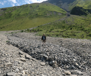
The self-channelization process is important because it prevents lateral spreading, maintaining the flow depth and hence the flow mobility for longer. This can significantly extend the overall run-out distance (Goujon, Dalloz-Dubrujeaud & Thomas Reference Goujon, Dalloz-Dubrujeaud and Thomas2007; Kokelaar et al. Reference Kokelaar, Graham, Gray and Vallance2014). Coarse-fragment-rich debris flows commonly self-channelize as they move on to shallower slopes (Iverson & Vallance Reference Iverson and Vallance2001; Félix & Thomas Reference Félix and Thomas2004; Johnson et al. Reference Johnson, Kokelaar, Iverson, Logan, LaHusen and Gray2012). Figure 2(a) shows an example from the bottom of the Biregrabe on the Albristore, near Färmelberg, Switzerland. There is a coarse-grained snout, as well as parallel-sided levees that are almost entirely composed of similar material. The levees are approximately 4 m apart and extend about 217 m upstream on a  $10^\circ$ slope, to where this small flow was diverted out of the main channel. As the flow waned, the central channel drained almost completely, leaving just the levees as evidence of the debris flow's path (figure 2b). Much larger debris flows occurred in this area on the 20 August 2012 and 24 July 2015, due to melting permafrost and high rainfall (C. Berger, personal communication). The deposits shown in figure 2 are interesting because the snout (which is often washed out by subsequent rainfall) has been almost perfectly preserved. It was deposits such as this and other observations of flowing debris flows that inspired Laigle & Bardou (Reference Laigle and Bardou2022) to draw their schematic diagram shown here in figure 1.
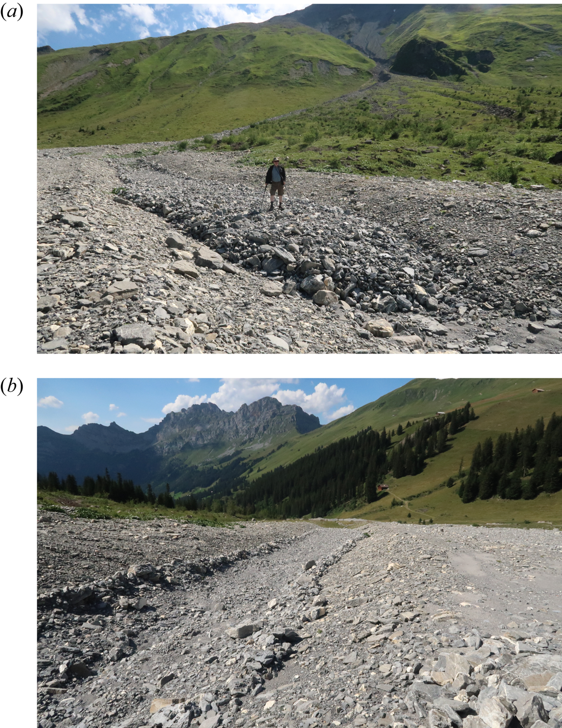
Figure 2. (a) Self-channelized flow front deposited at the bottom of the Biregrabe on the Albristore, near Färmelberg, Switzerland (latitude  $46^\circ 30'43.43"$ N, longitude $7^\circ 29'40.17"$ E, elevation 1775 m, slope ${\sim }10^\circ$). This area experienced large debris flows on the 20 August 2012 and 24 July 2015 due to melting permafrost and high rainfall (C. Berger, personal communication). This smaller deposit formed between 2017 and 2018. (b) Parallel-sided levees (approximately 4 m apart) left stranded at the side of the central channel as the flow waned.
Self-channelization also occurs in other geophysical mass flows, such as in the dense basal layer of pyroclastic flows, water-saturated lahars and wet snow avalanches (Rowley, Kuntz & MacLeod Reference Rowley, Kuntz and MacLeod1981; Wilson & Head Reference Wilson and Head1981; Branney & Kokelaar Reference Branney and Kokelaar1992; Calder, Sparks & Gardeweg Reference Calder, Sparks and Gardeweg2000; Vallance Reference Vallance2000; Jomelli & Bertran Reference Jomelli and Bertran2001; Jessop et al. Reference Jessop, Kelfoun, Labazuy, Mangeney, Roche and Tillier2012; Ancey Reference Ancey2012; Bartelt et al. Reference Bartelt, Glover, Feistl, Bühler and Buser2012; Schweizer, Bartelt & Van Herwijnen Reference Schweizer, Bartelt and Van Herwijnen2014; Vallance & Iverson Reference Vallance and Iverson2015). Although these flows contain fluid, which helps to mobilize them, self-channelization is not dependent on the presence of the fluid. Kokelaar et al. (Reference Kokelaar, Bahia, Joy, Viroulet and Gray2017) identified strongly leveed, fingered rock avalanche deposits in the southeast sector of Bessel crater in Mare Serenitatis on the Moon (see their figure 10). The fronts of these flows came to rest on a  ${\sim }31.5^\circ$ slope, and all of them look remarkably similar to the Biregrabe deposit in figure 2. These flows occurred in the complete absence of water or atmosphere. Interstitial fluids may therefore modify the frictional properties and significantly enhance the flow's mobility (Iverson & George Reference Iverson and George2014; Meng, Johnson & Gray Reference Meng, Johnson and Gray2022), but they are not necessary for a flow to self channelize on a suitably inclined slope.
Félix & Thomas (Reference Félix and Thomas2004) were able to generate leveed channels in small-scale analogue experiments with monodisperse dry grains. This showed that although particle-size segregation commonly occurs (and may be very important), it is not fundamentally necessary to generate a self-channelized flow. The coexistence of layers of static and flowing grains of similar thickness and at the same inclination angle, led Félix & Thomas (Reference Félix and Thomas2004) to suggest that self-channelization was related to frictional hysteresis. Frictional hysteresis (Daerr & Douady Reference Daerr and Douady1999) is responsible for the effect that when a steady uniform flow is brought to rest on a rough bed, a layer of grains of thickness  $h=h_{stop}(\zeta )$ is deposited at a slope angle $\zeta$, but this layer does not start to flow again until the chute is inclined to a higher angle $\zeta _{start}(h)>\zeta$. Pouliquen & Forterre (Reference Pouliquen and Forterre2002) showed how to capture this phenomenon by defining a non-monotonic basal friction law in a depth-averaged avalanche model. This friction law had (i) a multivalued static regime, (ii) a monotonically decreasing intermediate regime and (iii) a monotonically increasing dynamic regime, as a function of Froude number over the flow thickness. This friction law allowed static and flowing states to coexist for thicknesses in the range $h\in [h_{stop}(\zeta ), h_{start}(\zeta )]$, where $h_{start}(\zeta )$ is the inverse function of $\zeta _{start}(h)$.
Mangeney et al. (Reference Mangeney, Bouchut, Thomas, Vilotte and Bristeau2007) incorporated Pouliquen & Forterre's (Reference Pouliquen and Forterre2002) friction law into a depth-averaged avalanche model, and solved the system of equations numerically to show that it could generate a self-channelized flow with static levees. However, it was unclear what selected the width and height of the ensuing channel, which had multiple steady-state solutions. This contradicted the experimental evidence, which shows that for a given mass flux there is a well-defined channel width and height (Félix & Thomas Reference Félix and Thomas2004; Deboeuf et al. Reference Deboeuf, Lajeunesse, Dauchot and Andreotti2006; Takagi, McElwaine & Huppert Reference Takagi, McElwaine and Huppert2011; Rocha, Johnson & Gray Reference Rocha, Johnson and Gray2019). This conundrum was solved by Rocha et al. (Reference Rocha, Johnson and Gray2019), who incorporated additional depth-averaged in-plane viscous terms (Gray & Edwards Reference Gray and Edwards2014; Baker, Barker & Gray Reference Baker, Barker and Gray2016a), which generate a downslope velocity profile across the central channel. This provides the missing length scale that selects the steady-state flow height and the channel width. Rocha et al. (Reference Rocha, Johnson and Gray2019) showed that the resulting model was able to quantitatively capture experimental measurements of flow height and channel width as a function of the mass flux for quasi-monodisperse ( $0.45\pm 0.15$ mm) dry sand (Félix & Thomas Reference Félix and Thomas2004; Takagi et al. Reference Takagi, McElwaine and Huppert2011). Moreover, at low mass fluxes, Rocha et al. (Reference Rocha, Johnson and Gray2019) also correctly showed that self-channelized flows become unstable, and break down into a series of ‘erosion–deposition’ waves (Takagi et al. Reference Takagi, McElwaine and Huppert2011; Edwards & Gray Reference Edwards and Gray2015; Edwards et al. Reference Edwards, Viroulet, Kokelaar and Gray2017, Reference Edwards, Russell, Johnson and Gray2019). Similar surge waves that progressively erode and deposit previously fluidized material along their path are also commonly observed in debris flows (McArdell Reference McArdell2016).
The dynamic part of the non-monotonic friction law is intimately linked to the  $\mu (I)$ rheology for dry granular flows (GDR-Midi 2004; Jop, Forterre & Pouliquen Reference Jop, Forterre and Pouliquen2005, Reference Jop, Forterre and Pouliquen2006; Gray & Edwards Reference Gray and Edwards2014; Baker et al. Reference Baker, Barker and Gray2016a). Rather than having a constant Coulomb friction, the $\mu (I)$ rheology introduces rate dependence by making the friction $\mu$ a function of the inertial number
 \begin{equation} I=\frac{\dot{\gamma} d}{\sqrt{p/\rho_*}}, \end{equation}
where  $\dot {\gamma }$ is the shear rate, $d$ is the particle diameter, $p$ is the granular pressure and $\rho _*$ is the intrinsic density of the grains. This has spawned intense interest in the rheology of dry granular flows, as it provides a promising way of modelling chute flows, column collapses, silos and flows in rotating drums (GDR-Midi 2004; Jop et al. Reference Jop, Forterre and Pouliquen2006; Lagrée, Staron & Popinet Reference Lagrée, Staron and Popinet2011; Staron, Lagrée & Popinet Reference Staron, Lagrée and Popinet2012; Barker et al. Reference Barker, Schaeffer, Bohórquez and Gray2015; Barker & Gray Reference Barker and Gray2017; Martin et al. Reference Martin, Ionescu, Mangeney, Bouchut and Farin2017; Schaeffer et al. Reference Schaeffer, Barker, Tsuji, Gremaud, Shearer and Gray2019; Barker et al. Reference Barker, Rauter, Maguire, Johnson and Gray2021). The $\mu (I)$ rheology does not, however, capture the formation of $h_{stop}$ or $h_{start}$ layers. This phenomenology appears to be a non-local effect in which the ability of grains to flow, or not, is affected by motion some distance away (Schall & Van Hecke Reference Schall and Van Hecke2010). In the case of $h_{stop}$ and $h_{start}$ layers, it is the proximity of the fixed basal boundary to the free surface that has a strong effect on the ability of the grains to remain stable. An alternative approach (to the depth-averaged one used in this paper) is therefore to use one of the non-local models for granular flow (Pouliquen & Forterre Reference Pouliquen and Forterre2009; Kamrin & Koval Reference Kamrin and Koval2012; Bouzid et al. Reference Bouzid, Trulsson, Claudin, Clément and Andreotti2013, Reference Bouzid, Izzet, Trulsson, Clément, Claudin and Andreotti2015; Kamrin & Henann Reference Kamrin and Henann2015). In particular, Mowlavi & Kamrin (Reference Mowlavi and Kamrin2021) have recently captured both the $h_{stop}$, $h_{start}$ phenomenology in one-dimensional time-dependent simulations with a non-local model that includes hysteresis. Applying such models in three dimensions to capture self-channelization and levee formation remains, however, a significant challenge for the future.
If the relatively simple monodisperse depth-averaged model of Rocha et al. (Reference Rocha, Johnson and Gray2019) can quantitatively capture the self-channelization process, one may reasonably ask: (i) what is the role of particle segregation and (ii) does the small-scale experimental evidence have any bearing on large-scale geophysical flows? Interestingly, the strongly leveed, fingered rock avalanche deposits that Kokelaar et al. (Reference Kokelaar, Bahia, Joy, Viroulet and Gray2017) identified in the Bessel crater, look almost identical to small-scale segregation induced fingering experiments of Pouliquen, Delour & Savage (Reference Pouliquen, Delour and Savage1997), Woodhouse et al. (Reference Woodhouse, Thornton, Johnson, Kokelaar and Gray2012) and Baker, Johnson & Gray (Reference Baker, Johnson and Gray2016b). This led Kokelaar et al. (Reference Kokelaar, Bahia, Joy, Viroulet and Gray2017) to develop a scaling argument to show that the depth-averaged system of equations used by Baker et al. (Reference Baker, Johnson and Gray2016b) (which is similar to the model of Rocha et al. (Reference Rocha, Johnson and Gray2019), but includes the depth-averaged effect of segregation) scales with gravity  $g$ and a typical grain diameter $d$. Large-scale segregating bouldery dry flows on the Moon are therefore closely similar to small-scale dry flows with millimetre-sized particles on Earth.
In geophysical flows, the range of particle sizes is very wide, with particle diameters varying by several orders of magnitude. This allows particles to pack much more densely than monodisperse flows even during shear, which reduces the rate of segregation, and can lead to intermediate and reverse segregation for very large intruders (Thomas Reference Thomas2000). Such effects not only introduce bulk compressibility, but are still well beyond the scope of current granular rheologies and polydisperse particle-size segregation models (Gray & Ancey Reference Gray and Ancey2011; Marks, Rognon & Einav Reference Marks, Rognon and Einav2012; Gray Reference Gray2018; Barker et al. Reference Barker, Rauter, Maguire, Johnson and Gray2021). Indeed, until recently the segregation and diffusion rates in bidisperse segregation models (even with relatively small grains-size ratios) were poorly constrained (Golick & Daniels Reference Golick and Daniels2009; Thornton et al. Reference Thornton, Weinhart, Luding and Bokhove2012; Fan et al. Reference Fan, Schlick, Umbanhowar, Ottino and Lueptow2014; Hill & Tan Reference Hill and Tan2014; Schlick et al. Reference Schlick, Fan, Umbanhowar, Ottino and Lueptow2015; van der Vaart et al. Reference van der Vaart, Gajjar, Epely-Chauvin, Andreini, Gray and Ancey2015; Fry et al. Reference Fry, Umbanhowar, Ottino and Lueptow2019). As one of the first papers to investigate particle segregation in a non-trivial three-dimensional flow field, this paper uses a simple bidisperse model with the empirical segregation law of Trewhela, Ancey & Gray (Reference Trewhela, Ancey and Gray2021). Trewhela et al. (Reference Trewhela, Ancey and Gray2021) used refractive-index-matched shear-box experiments to track the segregation of large and small intruders as a function of time, and determined a scaling law that could collapse all their data. For grain-size ratios close to unity, they found that the segregation velocity magnitude is linearly dependent on the shear rate, the intrinsic particle density, the gravitational acceleration, the square of the average grain diameter and the deviation of the grain-size ratio away from unity, and inversely proportional to the pressure. Additional corrections, which are necessary at moderate grain-size ratios when the percolation of small intruders can be enhanced due to the spontaneous percolation, are ignored here, as are enhanced packing effects at large size ratios.
The inclusion of interstitial fluid also introduces additional complexity. For example, differentially fluidized regions of the flow will produce differential friction, which provides another mechanism to generate self-channelization without invoking frictional hysteresis. In particular, drier coarse-grained flow fronts and lateral levees will experience more friction than the fluid-saturated channel (Sharp & Nobles Reference Sharp and Nobles1953; Wilson & Head Reference Wilson and Head1981; Costa & Williams Reference Costa and Williams1984; Iverson & Vallance Reference Iverson and Vallance2001; Iverson Reference Iverson2003). This inhomogeneous rheology may well prove to be crucial at geophysical scale. In general, mixtures of grains and water can form suspensions whose friction  $\mu =\mu (J)$ is dependent on the viscous inertial number $J=\eta _f\dot {\gamma }/p^p$, where $\eta _f$ is the fluid viscosity and $p^p$ is the particle pressure (Boyer, Guazzelli & Pouliquen Reference Boyer, Guazzelli and Pouliquen2011). This constitutive law is valid for slow flows or small non-colloidal particles. As the shear rate is increased, the flow can transition from viscous inertial to granular inertial regimes with the friction $\mu =\mu (K)$, where $K=J+\alpha I^2$ is a combination of the viscous and granular inertial numbers and $\alpha$ is a constant, approximately equal to $0.1$ (Tapia et al. Reference Tapia, Ichihara, Pouliquen and Guazzelli2022). The ratio $I^2/J=\rho _*d^2\dot {\gamma }/\eta _f$ defines a Stokes number $St$, which is particle-size dependent, and governs the extent to which the particles are affected by the fluid. If $St\gg 1/\alpha$, then the particles are affected by fluid buoyancy, but do not closely follow fluid streamlines and in dense flows, they are in the inertial granular regime (Maurin, Chauchat & Frey Reference Maurin, Chauchat and Frey2016). Particles with $St\ll 1/\alpha$ are strongly affected by the fluid and are in the viscous inertial regime. For debris flows, where there is a wide range of grain sizes, it is likely that the rocks and coarse-grained sand are in the inertial granular regime, while the very finest grains will be in the viscous inertial regime. The implicit assumption in this paper is that the larger grains dominate the overall debris-flow response, and hence the $\mu (I)$ rheology is most appropriate (GDR-Midi 2004; Jop et al. Reference Jop, Forterre and Pouliquen2006; Gray & Edwards Reference Gray and Edwards2014).
In depth-averaged two-phase-flow models, the primary effect of the fluid is the buoyancy-induced reduction in the granular friction, which may additionally be enhanced by excess pore-pressure effects (Iverson & Denlinger Reference Iverson and Denlinger2001; Pitman & Le Reference Pitman and Le2005; Pelanti, Bouchut & Mangeney Reference Pelanti, Bouchut and Mangeney2008; Pudasaini Reference Pudasaini2012; Iverson & George Reference Iverson and George2014; Meng & Wang Reference Meng and Wang2016; Meng et al. Reference Meng, Johnson and Gray2022). These allow debris flows to propagate over much shallower slopes than dry granular materials, as in the debris flow at Färmelberg (figure 2). However, on these shallower slopes, the resulting flow dynamics and observed deposit morphologies are closely similar to the dry small-scale experiments (Sharp & Nobles Reference Sharp and Nobles1953; Wilson & Head Reference Wilson and Head1981; Costa & Williams Reference Costa and Williams1984; Branney & Kokelaar Reference Branney and Kokelaar1992; Iverson Reference Iverson1997; Major Reference Major1997; Major & Iverson Reference Major and Iverson1999; Calder et al. Reference Calder, Sparks and Gardeweg2000; Iverson & Vallance Reference Iverson and Vallance2001; Iverson Reference Iverson2003; Félix & Thomas Reference Félix and Thomas2004; Iverson et al. Reference Iverson, Logan, LaHusen and Berti2010; Takagi et al. Reference Takagi, McElwaine and Huppert2011; Johnson et al. Reference Johnson, Kokelaar, Iverson, Logan, LaHusen and Gray2012; Kokelaar et al. Reference Kokelaar, Graham, Gray and Vallance2014; Rocha et al. Reference Rocha, Johnson and Gray2019).
The aim of this paper is to study the segregation in a representative three-dimensional self-channelizing flow field (Rocha et al. Reference Rocha, Johnson and Gray2019). A specific example is chosen which scales up (Kokelaar et al. Reference Kokelaar, Bahia, Joy, Viroulet and Gray2017) to look qualitatively similar to the large-scale experimental debris flows at the United States Geological Survey (USGS) flume (Iverson et al. Reference Iverson, Logan, LaHusen and Berti2010; Johnson et al. Reference Johnson, Kokelaar, Iverson, Logan, LaHusen and Gray2012). This flow field therefore provides a generic test case. In § 2, the depth-averaged theory of Rocha et al. (Reference Rocha, Johnson and Gray2019) is introduced, and this is used in § 3 to compute a two-dimensional travelling wave solution for the process of self-channelization. In § 4, incompressibility and assumed velocity profiles are used to reconstruct a realistic flow field for self-channelization in three dimensions. This flow field is then held fixed for the remainder of the paper.
Our study is motivated by the USGS debris-flow experiments (Johnson et al. Reference Johnson, Kokelaar, Iverson, Logan, LaHusen and Gray2012) and the experiments of Kokelaar et al. (Reference Kokelaar, Graham, Gray and Vallance2014), which both had quite tightly constrained particle-size distributions. In the bidisperse small-scale experiments, Kokelaar et al. (Reference Kokelaar, Graham, Gray and Vallance2014) used mixtures of glass ballotini and carborundum, and glass ballotini and sand, with size ratios of approximately 1.81 and 1.63, respectively. The flume experiments had a more realistic continuous grain-size distribution ranging from  $100\ \mathrm {\mu }{\rm m}$ to 32 mm, but the most pronounced segregation occurred between grains of modest size ratio ( ${<}5$). Kokelaar et al. (Reference Kokelaar, Graham, Gray and Vallance2014) used a resin impregnation and sectioning technique to reveal the internal particle-size distribution within the levees and the central channel. The levees were not entirely composed of large grains, as one might anticipate from surface observations, but had an inner core of fine grains. Fine grains also line the inside of the channel. Experimental measurements of the run-out distance as a function of flow composition led Kokelaar et al. (Reference Kokelaar, Graham, Gray and Vallance2014) to infer that it was the formation of levees and a fine particle channel lining that led to the maximum run out with 60–70 % fines. This was first because the $\mu (I)$ rheology implies that a finer-grained flow experiences less friction (for grains of the same shape), and can flow further and faster, than a larger grained flow of the same depth (GDR-Midi 2004; Rognon et al. Reference Rognon, Roux, Naaim and Chevoir2007; Barker et al. Reference Barker, Rauter, Maguire, Johnson and Gray2021), and second because lateral confinement maintains flow depth, and hence mobility, for longer. Flows of pure fine grains at the same slope angle do not self-channelize, instead spreading laterally and stopping more rapidly (Kokelaar et al. Reference Kokelaar, Graham, Gray and Vallance2014). In debris flows and pyroclastic flows, fine grains additionally hinder the escape of water and gas, and thereby help to maintain high pore pressures, which also convey mobility to the flow (Iverson Reference Iverson2003). The particle-size distribution can therefore have a profound effect on the bulk flow behaviour, and this paper seeks to understand how it develops in the three-dimensional self-channelizing flow field developed in § 4. In § 5, a state-of-the-art particle segregation model (Gray Reference Gray2018; Barker et al. Reference Barker, Rauter, Maguire, Johnson and Gray2021) is introduced that uses Trewhela et al.'s (Reference Trewhela, Ancey and Gray2021) empirical segregation law. Fully three-dimensional, time-dependent, numerical solutions for the particle-size distribution in the vicinity of the moving front are then computed in § 6. The dependence on the grain-size ratio and the inflow concentration are investigated in § 7, and § 8 concludes.
2. Depth-averaged model for self-channelization
2.1. Governing equations
Granular material is supplied from a point source onto a rough plane that is inclined at an angle  $\zeta$ to the horizontal. A Cartesian coordinate system $Oxyz$ is defined with the origin $O$ located at the top centre of the plane. The $x$-axis points downslope, the $y$-axis points across the slope and the $z$-axis is the upward pointing normal. The unit normals are $\boldsymbol {e}_x$, $\boldsymbol {e}_y$ and $\boldsymbol {e}_z$, and the velocity $\boldsymbol {u}$ has components $(u,v,w)$ in each of these three directions, respectively. The equations are integrated through the flow depth $h$, measured normal to the plane, and the depth-averaged velocity $\bar {\boldsymbol {u}}$ has components
 \begin{equation} \bar{u} = \frac{1}{h}\int_0^h u\,\mathrm{d}z, \quad \bar{v} = \frac{1}{h}\int_0^h v\,\mathrm{d}z, \end{equation}
in the downslope and cross-slope directions, respectively. The granular material is assumed to be incompressible with a constant-uniform bulk density  $\rho$. It follows that the depth-averaged mass and momentum balance equations (Gray & Edwards Reference Gray and Edwards2014; Baker et al. Reference Baker, Barker and Gray2016a; Edwards et al. Reference Edwards, Viroulet, Kokelaar and Gray2017) are
 $$\begin{gather} \dfrac{\partial{h}}{\partial{t}} + \mbox{div}\left(h \bar{\boldsymbol{u}}\right) = 0, \end{gather}$$
 $$\begin{gather} \dfrac{\partial}{\partial{t}}\left(h\bar{\boldsymbol{u}}\right) + \mbox{div}\left(h \bar{\boldsymbol{u}} \otimes \bar{\boldsymbol{u}}\right) + \mbox{grad}\left(\frac{1}{2} h^2 g\cos{\zeta}\right) = hg\boldsymbol{S} \cos{\zeta} + \hbox{div}\left(\nu h^{3/2}\bar{\boldsymbol{D}}\right), \end{gather}$$
where  $\otimes$ is the dyadic product and $g$ is the constant of gravitational acceleration. Note that the two-dimensional divergence and gradient operators, $\hbox {div}$ and $\hbox {grad}$, are used here to distinguish them from their three-dimensional counterparts, which are written in terms of the $\boldsymbol {\nabla }$ operator in § 5. In the source term on the right-hand side of (2.3), the non-dimensional net acceleration,
 \begin{equation} \boldsymbol{S} = \tan{\zeta}\,\boldsymbol{e_x} - \mu_b\boldsymbol{e}, \end{equation}
consists of the component of gravity pulling the avalanche downslope along the direction of the unit vector  $\boldsymbol {e}_x$ and the effective basal friction $\mu _b$. The hysteretic effective basal friction law for $\mu _b$ is introduced in § 2.2. It is a generalization of Pouliquen's (Reference Pouliquen1999a) dynamic friction law, which is directly linked to the $\mu (I)$ rheology for granular flows (GDR-Midi 2004; Jop et al. Reference Jop, Forterre and Pouliquen2005, Reference Jop, Forterre and Pouliquen2006; Gray & Edwards Reference Gray and Edwards2014; Baker et al. Reference Baker, Barker and Gray2016a). If the avalanche is in motion, the direction of the friction, $\boldsymbol {e}$, opposes the motion, and when the grains are static, the friction opposes the downslope component of gravitational acceleration and the depth-averaged pressure gradient, which implies that
 \begin{equation} \boldsymbol{e} = \begin{cases} \dfrac{\bar{\boldsymbol{u}}}{|\bar{\boldsymbol{u}}|} & \text{if $|\bar{\boldsymbol{u}}|>0$},\\[10pt] \dfrac{\tan\zeta\,\boldsymbol{e}_x-\hbox{grad}\,h}{|\tan\zeta\,\boldsymbol{e}_x-\hbox{grad}\,h|} & \text{if $|\bar{\boldsymbol{u}}|=0$}. \end{cases} \end{equation}
The final term on the right-hand side of (2.3) arises from the inclusion of depth-averaged in-plane deviatoric stresses, which are neglected in most theories. Here, however, they play a crucial role in selecting a unique solution for the steady-state channel width and height. Gray & Edwards (Reference Gray and Edwards2014) and Baker et al. (Reference Baker, Barker and Gray2016a) derived the specific form for this second-order-gradient depth-averaged viscous term from the  $\mu (I)$ rheology. It consists of a depth-averaged viscosity $\nu h^{1/2}/2$ that multiplies the depth-integrated strain-rate tensor
 \begin{equation} \bar{\boldsymbol{D}} = \tfrac{1}{2}\left(\bar{\boldsymbol{L}} + \bar{\boldsymbol{L}}^{T}\right), \end{equation}
where  $\bar {\boldsymbol {L}}=\hbox {grad}\,\bar {\boldsymbol {u}}$ is the two-dimensional gradient of the depth-averaged velocity. The coefficient $\nu$ is determined from the $\mu (I)$ friction law (GDR-Midi 2004; Jop et al. Reference Jop, Forterre and Pouliquen2006) and an explicit formula will be given for it in § 2.3.
2.2. The hysteretic friction law
This paper uses the hysteretic friction law of Edwards et al. (Reference Edwards, Russell, Johnson and Gray2019), which is a generalization of Pouliquen & Forterre's (Reference Pouliquen and Forterre2002) original law. It consists of three cases that are known as the dynamic, intermediate and static friction regimes
 \begin{equation}
\mu_b(h/d,Fr)=\left\{ \begin{array}{@{}ll@{}} \mu_{D}, & Fr
\geqslant \beta_*, \\ \mu_{I}, & 0 < Fr \leqslant
\beta_*,\\ \mu_{S}, & Fr=0. \end{array}\right.
\end{equation}
\begin{equation}
\mu_b(h/d,Fr)=\left\{ \begin{array}{@{}ll@{}} \mu_{D}, & Fr
\geqslant \beta_*, \\ \mu_{I}, & 0 < Fr \leqslant
\beta_*,\\ \mu_{S}, & Fr=0. \end{array}\right.
\end{equation}These regimes are defined respectively by the functions
 $$\begin{gather} \mu_{D}=\mu_1 + \frac{\mu_2 - \mu_1}{1 + h \beta/(\mathcal{L}d(Fr+\varGamma))}, \end{gather}$$
 $$\begin{gather}\mu_{I}=\left(\dfrac{Fr}{\beta_*}\right)\left(\mu_1 + \frac{\mu_2 - \mu_1}{1 + h \beta/(\mathcal{L}d(\beta_*+\varGamma))} - \mu_3-\frac{\mu_2 - \mu_1}{1 + h /(\mathcal{L}d)}\right) + \mu_3 + \frac{\mu_2 - \mu_1}{1 + h /(\mathcal{L}d)}, \end{gather}$$
 $$\begin{gather}\mu_{S}=\textrm{min}\left( \mu_3 + \frac{\mu_2 - \mu_1}{1 + h /(\mathcal{L}d)}, |\tan \zeta\,\boldsymbol{e}_x-\hbox{grad}\,h| \right), \end{gather}$$
where  $\mu _1=\tan \zeta _1$, $\mu _2=\tan \zeta _2$ and $\mu _3=\tan \zeta _3$ are the tangents of the friction angles $\zeta _1$, $\zeta _2$ and $\zeta _3$. These parameters are determined from experimental fits to the deposit depth $h_{stop}(\zeta )$ and initiation thickness $h_{start}(\zeta )$ as a function of $\zeta$. The fitting functions contain a frictional length scale $\mathscr {L}$, which Forterre & Pouliquen (Reference Forterre and Pouliquen2003) showed scales with the grain size $d$. This grain-size dependence has explicitly been included in (2.8)–(2.10) by defining the non-dimensional friction length scale $\mathcal {L}=\mathscr {L}/d$. The regime boundaries are determined by the Froude number $Fr$, which is the ratio of the flow speed to the gravity wave speed
 \begin{equation} Fr=\frac{|\bar{\boldsymbol{u}}|}{\sqrt{gh\cos\zeta}}. \end{equation}
If  $Fr$ is above the minimum Froude number $\beta _*$ for steady-uniform flow, then the flow is in the dynamic regime, if the Froude number equals zero, it is in the static regime and if $Fr\in (0,\beta _*)$, then it is in the intermediate regime. The remaining non-dimensional constants $\beta$ and $\varGamma$ are determined from a pair of best fits to the steady-uniform-flow law for angular particles (Forterre & Pouliquen Reference Forterre and Pouliquen2003)
 \begin{equation} Fr = \beta \frac{h}{h_{stop}} - \varGamma. \end{equation}
Edwards et al. (Reference Edwards, Russell, Johnson and Gray2019) assumed that the minimum observable steady-uniform flow occurs at the same Froude number  $Fr=\beta _*$ at all slope angles. It follows from (2.12) that the minimum steady-uniform-flow depth
 \begin{equation} h_* = \left(\frac{\beta_*+\varGamma}{\beta}\right) h_{stop}(\zeta), \end{equation}
which implies that  $h_*$ is a multiple of $h_{stop}$. The frictional parameters must be chosen so that $h_{stop}< h_*< h_{start}$ for the hysteretic friction law to be well defined. A necessary, but not sufficient condition is that $\mu _1<\mu _3<\mu _2$. This paper adopts the parameters for sand used by Rocha et al. (Reference Rocha, Johnson and Gray2019), except for $\zeta _3$, which is increased from $31^\circ$ to $33^\circ$. This increases the maximum static friction and hence the thickness range $(h\in [h_{stop},h_{start}])$ with coexisting flowing and static states. Increasing $\mu _3$ gives the levees slightly greater stability than in the simulations of Rocha et al. (Reference Rocha, Johnson and Gray2019), which suppresses the periodically upslope propagating erosion-deposition waves seen in their movie 5. All the parameters (see table 1) are tightly constrained by existing experiments in the literature and are typical of those for sand flowing on a bed of glass beads. Rocha et al. (Reference Rocha, Johnson and Gray2019) also gave parameters for flows of glass beads, which also form levees even though $\varGamma =0$ (Félix & Thomas Reference Félix and Thomas2004). The values of $\mu _1$ and $\mu _3$ are, however, very close to one another, which leads to weak non-monotonic dependence of the friction $\mu$ on the Froude number $Fr$, as shown in figure 6(b) of Rocha et al. (Reference Rocha, Johnson and Gray2019). This leads to very weak levees. Indeed, Deboeuf et al. (Reference Deboeuf, Lajeunesse, Dauchot and Andreotti2006) have observed experimentally that levees of glass beads slowly creep outwards over very long periods of time, which is not the case for sand.
Table 1. Material properties for flows of sand with a mean diameter of  $0.45$ mm. The values of $\zeta _1$, $\zeta _2$ and $\mathcal {L}$ were calculated from the $h_{stop}$ curve of Takagi et al. (Reference Takagi, McElwaine and Huppert2011) by Rocha et al. (Reference Rocha, Johnson and Gray2019). The values of $\beta$ and $\varGamma$ differ from those in Pouliquen & Forterre (Reference Pouliquen and Forterre2002) and Forterre & Pouliquen (Reference Forterre and Pouliquen2003) to account for the factor $\sqrt {\cos \zeta }$ in the Froude number (2.11). All the values are the same as those used by Rocha et al. (Reference Rocha, Johnson and Gray2019) except for $\zeta _3$, which is increased from $31^\circ$ to $33^\circ$ to give the sand slightly more stability in the hysteretic flow regime.
2.3. The coefficient  $\nu$
$\nu$

Gray & Edwards (Reference Gray and Edwards2014) and Baker et al. (Reference Baker, Barker and Gray2016a) derived the depth-averaged viscous terms in (2.3) from the  $\mu (I)$ rheology (GDR-Midi 2004; Jop et al. Reference Jop, Forterre and Pouliquen2006). In this equation, the coefficient
 \begin{equation} \nu = \frac{2}{9} \frac{\mathcal{L}d\sqrt{g}}{\beta} \frac{\sin{\zeta}}{\sqrt{\cos{\zeta}}} \left( \frac{\mu_2 - \tan{\zeta}}{\tan{\zeta} - \mu_1} \right), \end{equation}
is explicitly determined during the integration process in terms of the existing friction parameters, summarized in table 1, and the slope angle  $\zeta$. Equation (2.14) is valid for slope inclinations in the range $\zeta \in [\zeta _1,\zeta _2]$, when steady-uniform flows are predicted to exist by the dynamic frictional law (2.8). In reality, the lowest observable steady-uniform flow occurs at $Fr=\beta _*$ and one might anticipate that the form of $\nu$ might change when the flow is in the intermediate (2.9) and static (2.10) regimes. However, in the computations presented in this paper, (2.14) is assumed to apply to all regimes.
2.4. Particle size and gravitational dependence
The governing equations can be made non-dimensional by introducing scalings based on a typical particle diameter  $d$ and gravity $g$
$g$
 \begin{equation}
\left.\begin{array}{@{}c@{}} (x,y,z,h)=d\,(\tilde{x}, \tilde{y},
\tilde{z}, \tilde{h}),\quad t=\sqrt{d/g}\,\tilde{t},\\
\bar{\boldsymbol{u}}=\sqrt{gd}\,\tilde{\bar{\boldsymbol{u}}},\quad
\bar{\boldsymbol{D}}=\sqrt{g/d}\,\tilde{\bar{\boldsymbol{D}}},\quad
\nu=d\sqrt{g}\,\tilde{\nu}, \end{array}\right\}
\end{equation}
\begin{equation}
\left.\begin{array}{@{}c@{}} (x,y,z,h)=d\,(\tilde{x}, \tilde{y},
\tilde{z}, \tilde{h}),\quad t=\sqrt{d/g}\,\tilde{t},\\
\bar{\boldsymbol{u}}=\sqrt{gd}\,\tilde{\bar{\boldsymbol{u}}},\quad
\bar{\boldsymbol{D}}=\sqrt{g/d}\,\tilde{\bar{\boldsymbol{D}}},\quad
\nu=d\sqrt{g}\,\tilde{\nu}, \end{array}\right\}
\end{equation}where the tilde is used to indicate a non-dimensional variable. It follows that the non-dimensional form of the mass and momentum balances (2.2) and (2.3) are
 $$\begin{gather} \dfrac{\partial{\tilde{h}}}{\partial{\tilde{t}}} + \widetilde{\hbox{div}}\left(\tilde{h} \tilde{\bar{\boldsymbol{u}}}\right) = 0, \end{gather}$$
 $$\begin{gather} \dfrac{\partial}{\partial{\tilde{t}}}\left(\tilde{h}\tilde{\bar{\boldsymbol{u}}}\right) + \widetilde{\hbox{div}}\left(\tilde{h} \tilde{\bar{\boldsymbol{u}}} \otimes \tilde{\bar{\boldsymbol{u}}}\right) + \widetilde{\hbox{grad}}\left(\frac{1}{2} \tilde{h}^2\cos{\zeta}\right) = \tilde{h}\boldsymbol{S} \cos{\zeta} + \widetilde{\hbox{div}}\left(\tilde{\nu} \tilde{h}^{3/2}\tilde{\bar{\boldsymbol{D}}}\right), \end{gather}$$
respectively, where  $\widetilde {\hbox {div}}$ and $\widetilde {\hbox {grad}}$ are the non-dimensionalized divergence and gradient operators and the non-dimensional coefficient in the viscous term
 \begin{equation} \tilde\nu = \frac{2}{9} \frac{\mathcal{L}}{\beta} \frac{\sin{\zeta}}{\sqrt{\cos{\zeta}}} \left( \frac{\mu_2 - \tan{\zeta}}{\tan{\zeta} - \mu_1} \right). \end{equation}
Moreover, the non-dimensional net acceleration  $\boldsymbol {S}$, the unit vector $\boldsymbol {e}$ and the friction $\mu _b$, defined in (2.4), (2.5) and (2.7), respectively, are already written in dimensionless form, since $\bar {\boldsymbol {u}}/|\bar {\boldsymbol {u}}|=\tilde {\bar {\boldsymbol {u}}}/|\tilde {\bar {\boldsymbol {u}}}|$, $\hbox {grad}\,h=\widetilde {\hbox {grad}}\,\tilde {h}$ and $\mu _b(h/d,Fr)=\mu _b(\tilde {h},Fr)$. The non-dimensional system of equations is therefore independent of any additional non-dimensional groups involving $d$ or $g$ dependence. These non-dimensionalized equations are therefore scale and gravity independent. This remarkable result is due to Kokelaar et al. (Reference Kokelaar, Bahia, Joy, Viroulet and Gray2017), and implies that provided all the length scales (height, width and length) scale up with the particle size, the results will be the same. A self-channelized geophysical flow of large boulders, such as that shown in figure 2, may therefore be exactly equivalent to a small-scale experimental flow involving millimetre-sized grains (Rocha et al. Reference Rocha, Johnson and Gray2019). This scaling on the particle size relies on the fact that the frictional length scale $\mathscr {L}=\mathcal {L}d$ scales linearly on $d$. Forterre & Pouliquen (Reference Forterre and Pouliquen2003) showed that $\mathscr {L}=1.65d$ for glass beads and $\mathscr {L}=2.03d$ for sand. In this paper, the non-dimensional frictional length $\mathcal {L}=\mathscr {L}/d$ is assumed to be equal to $2$ (table 1).
Kokelaar et al. (Reference Kokelaar, Bahia, Joy, Viroulet and Gray2017) applied these ideas to large-scale dry granular flows on the Moon, which occur during crater wall collapses. The reduced gravity on the Moon implies that the velocities will be slower than an equivalent sized flow on Earth and the flows would therefore have taken correspondingly longer to run out. However, Kokelaar et al.'s (Reference Kokelaar, Bahia, Joy, Viroulet and Gray2017) figure 10 shows self-channelized fingered deposits in the Bessel crater in Mare Serenitatis (latitude 21.8 $^\circ$N, longitude 17.9 $^\circ$E) that are closely analogous to the small-scale segregation induced fingering experiments of Pouliquen et al. (Reference Pouliquen, Delour and Savage1997), Woodhouse et al. (Reference Woodhouse, Thornton, Johnson, Kokelaar and Gray2012) and Baker et al. (Reference Baker, Johnson and Gray2016b). The presence of water in debris flows on Earth modifies the friction law and the scaling properties. However, the essential flow dynamics and morphological features remain closely similar as demonstrated by the USGS debris-flow-flume experiments (Johnson et al. Reference Johnson, Kokelaar, Iverson, Logan, LaHusen and Gray2012).
3. Depth-averaged simulations of a self-channelized flow
The governing equations in § 2 are now solved numerically to generate thickness and depth-averaged velocity fields that quantitatively capture the small-scale self-channelized flow experiments of Takagi et al. (Reference Takagi, McElwaine and Huppert2011) and Rocha et al. (Reference Rocha, Johnson and Gray2019). The scaling behaviour with particle size (see § 2.4) ensures that this solution is also appropriate for geophysical flows, whose average grain size is much larger than that in the small-scale experiments. The solution is then transformed to a frame of reference moving with the flow front, to show that over longer integration periods, a travelling-wave solution develops that is steady in the moving frame.
3.1. Continuous release of grains on an inclined plane
A numerical simulation is first performed to capture the continuous release of sand from a point source onto a rough plane inclined at  $\zeta =32^{\circ }$. The values of the critical thicknesses $h_{stop}$, $h_*$ and $h_{start}$ as well as $\nu$ are therefore constant, and their specific values are summarized in table 2. The computational domain consists of a rectangle covering the area $0\ {\rm m} \leqslant x \leqslant 2.5$ m and $-10\ {\rm cm} \leqslant y \leqslant 10$ cm, discretized to $2500\times 200$ finite volume cells (1 grid point per mm in both directions). The conservation equations (2.2) and (2.3) are solved numerically with a semi-discrete non-oscillatory central (NOC) scheme, which uses a generalized minmod limiter with $\theta =2$ (Kurganov & Tadmor Reference Kurganov and Tadmor2000). The time-stepping is performed with a second-order Runge–Kutta method, with the step size determined by a CFL (Courant–Friedrichs–Lewy) number of $0.225$ and limited to a maximum of $\Delta t = 10^{-4}$ s (LeVeque Reference LeVeque2002) to minimize the creep in the levees.
Table 2. Critical layer thicknesses  $h_{stop}$, $h_*$ and $h_{start}$ as well as the coefficient $\nu$ (in the depth-averaged viscosity $\nu h^{1/2}/2$) for the material properties for sand in table 1 and the fixed slope angle of $\zeta =32.0^{\circ }$ used in the numerical computations.
The initial conditions at  $t=0$ are $h=h_0=0.01$ mm (around 50 times smaller than the mean particle diameter) and $\bar {\boldsymbol {u}}=\boldsymbol {0}\ {\rm m}\ {\rm s}^{-1}$ everywhere. This thin static layer is required to mitigate numerical errors caused by the degeneracy of the governing equations at $h=0$. Following Rocha et al. (Reference Rocha, Johnson and Gray2019), a source term $S_{inflow}$ is included on the right-hand side of (2.2) to give
 \begin{equation} \dfrac{\partial{h}}{\partial{t}} + \hbox{div}\left(h \bar{\boldsymbol{u}}\right) = S_{inflow}, \end{equation}
which allows grains to be added in a small circular region of radius  $r_0=2.5$ cm centred at $(x_0,y_0)=(15$ cm $,0)$ at a flow rate of $Q_m = 130\ {\rm g}\ {\rm s}^{-1}$, i.e.
 \begin{equation} S_{inflow}=\left\{\begin{array}{@{}ll@{}} \displaystyle\dfrac{3 Q_M}{{\rm \pi} \rho r_0^6} \left(r_0^2 - \left((x-x_0)^2 + y^2\right) \right)^2, & (x-x_0)^2 + y^2 \leqslant r_0^2,\\[10pt] 0, & (x-x_0)^2 + y^2 > r_0^2. \end{array}\right. \end{equation}
The inflowing particles move downslope and some of them eventually reach the downstream boundary  $x=2.5$ m, where a free outflow condition is imposed by linear extrapolation of the values of $h$ and $h\bar {u}$ from the final two columns of interior cells. The conditions $h=h_0$ and $\bar {\boldsymbol {u}}=\boldsymbol {0}\ {\rm m}\ {\rm s}^{-1}$ are trivially satisfied at the top $x=0$ and sides $y= \pm 10$ cm of the domain where no flow reaches.
The results of this numerical simulation are plotted in figure 3 at times  $t=7$, $14$,
$14$,  $21$ and $28$ s. The continuous release of grains is shown to quickly form a self-channelized flow with static levees. In the central flowing channel, which is of approximately constant thickness $9$ mm and uniform width $16$ cm, material is transported towards the flow front. When it reaches the front, the lateral confinement is lost and the flow spreads out, rapidly coming to rest and building up new sections of the levees just behind the flow front. The levees are approximately $2.5$ cm wide and have a thickness that starts at the flowing channel depth and decreases to zero. As a result, the front in figure 3 appears to propagate steadily downslope at constant velocity $u_F \simeq 0.07\ {\rm m}\ {\rm s}^{-1}$, suggesting that a two-dimensional travelling wave is generated.
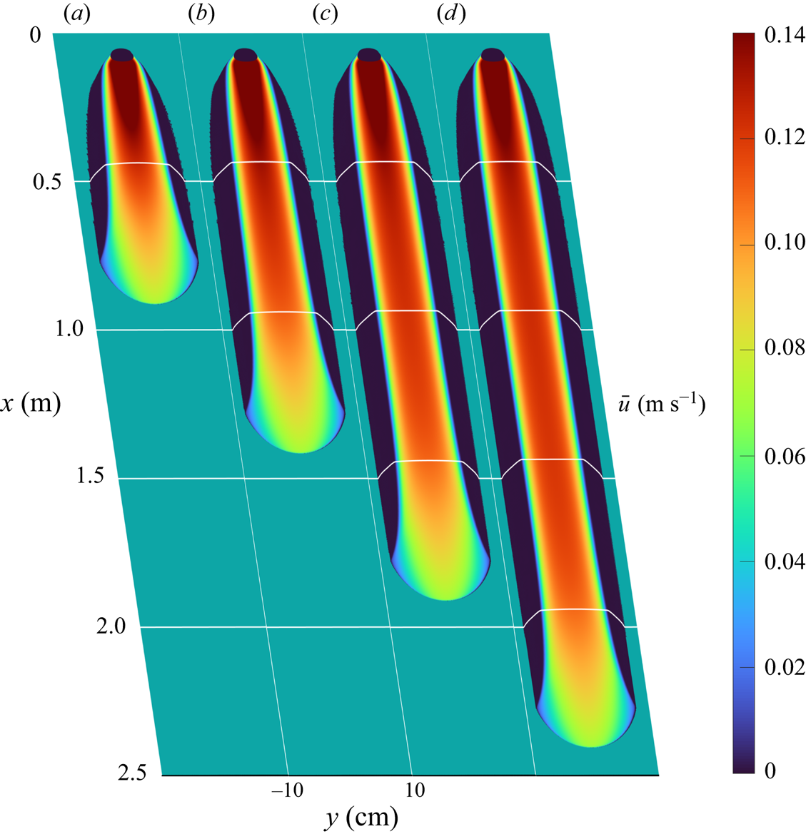
Figure 3. Surface plots of the flow thickness  $h$ for the numerical simulation of a release of particles at a flow rate of $Q_m = 130\ {\rm g}\ {\rm s}^{-1}$ on a plane inclined at $\zeta =32^{\circ }$, coloured by the downslope component of depth-averaged velocity $\bar {u}$ and shown at times (a) $t = 7$, (b) $14$, (c) $21$ and (d) $28$ s. The filled black circles indicate the non-zero source region where $S_{inflow}$ is given by (3.2) and the solid horizontal white lines indicate cross-slope flow thickness, mimicking the displacement of an experimental laser line. The online supplementary movie 1 available at https://doi.org/10.1017/jfm.2022.1089 shows the time dependent evolution of the flow.
3.2. Depth-averaged travelling frame simulation
For the travelling wave to be fully realised, it is useful to perform simulations in a frame moving at the front speed  $u_F$. Using the change of coordinates
 \begin{equation} \tau=t-t_0,\quad \xi = x - u_F t, \end{equation}
the mass and momentum conservation laws (2.2) and (2.3) can be written
 $$\begin{gather} \dfrac{\partial{h}}{\partial{\tau}} + \hbox{div}'\left(h \bar{\boldsymbol{u}}^{\prime}\right) = S'_{inflow}, \end{gather}$$
 $$\begin{gather} \dfrac{\partial}{\partial{\tau}}\left(h\boldsymbol{\bar{u}}^{\prime}\right) + \hbox{div}' \left(h \bar{\boldsymbol{u}}^{\prime} \otimes \bar{\boldsymbol{u}}^{\prime}\right) + \hbox{grad}'\left(\frac{1}{2} h^2 g\cos{\zeta}\right) = hg\boldsymbol{S} \cos{\zeta} + \hbox{div}'\left(\nu h^{3/2}\overline{\boldsymbol{D}^\prime}\right), \end{gather}$$
where  $\hbox {div}'$ and $\hbox {grad}'$ are now the two-dimensional divergence and gradient operators in the moving frame $(\xi,y)$. The depth-averaged velocity in the moving frame is equal to $\bar {\boldsymbol {u}}^{\prime } = \bar {\boldsymbol {u}}-u_F\boldsymbol {e}_x$. The strain-rate tensor is unchanged in the moving frame, i.e. $\bar {\boldsymbol {D}}^\prime =\bar {\boldsymbol {D}}$. Note that the elimination of $\bar {\boldsymbol {u}}$ in the transformed momentum balance (3.5) relies on subtracting $u_F$ times the moving frame mass balance (3.4) from the transformed downslope momentum balance.
Since (3.4) and (3.5) have the same structure as the original mass and momentum balance equations (2.2) and (2.3), the numerical method described in § 3.1 can be used to compute the flow in the moving frame. This time, the computational domain is a rectangle covering the area  $-0.8\ {\rm m} \leqslant \xi \leqslant 0.8$ m and $-10\ {\rm cm} \leqslant y \leqslant 10$ cm, discretized to $1600\times 200$ finite volume cells (with the same resolution of 1 grid point per mm in both directions as the continuous release simulation). The initial conditions at $\tau = 0$ are the $t = t_0 = 28$ s state of the continuous release simulation, which is shown in figure 3(d). At the downstream boundary, at $\xi = 0.8$ m, the precursor layer enters the domain with thickness $h=h_0$ and velocity $\bar {\boldsymbol {u}}^\prime =-u_F\boldsymbol {e}_x$, which is equivalent to zero velocity in the stationary frame. This condition is also trivially satisfied at the sides $y= \pm 10$ cm.
The upstream boundary condition is more complex. Physically, this is because some of the grains in the central channel are moving downslope towards the front, and therefore must enter the domain at  $\xi =-0.8$ m, whilst other grains at the sides and base of the central channel, as well as in the static levees, are moving slower than the front and leave the domain. This has to be accounted for in a depth-averaged model by allowing an inflow along part of the upstream boundary and an outflow along the rest. To achieve this, a novel procedure has been developed. First, the net mass flux leaving the domain across the upstream boundary is calculated by evaluating the integral
 \begin{equation} Q_{out} ={-}\rho\int_{{-}W/2}^{{+}W/2} h\bar{u}^{\prime} \rvert_{\xi={-}0.8\ {\rm m}}\, \mathrm{d}y. \end{equation}
At steady state, the inflowing and outflowing grains should be in exact balance and  $Q_{out}$ should equal zero. However, the initial state is not yet quite in steady state and therefore $Q_{out}$ is non-zero. To correct for the net loss/gain of particles across $\xi =-0.8$ m, a mass source term (similar to that applied in (3.1)) is applied across the first row of interior grid cells. The new source term in the moving frame simulations is therefore
 \begin{equation} S'_{inflow} = \dfrac{Q_{out}h\rvert_{\xi={-}0.8\ \mathrm{m}}}{\rho\Delta x \displaystyle\int\nolimits_{{-}W/2}^{{+}W/2} h\rvert_{\xi={-}0.8\ \mathrm{m}}\,\mathrm{d} y} \end{equation}
inside the first grid cell and zero otherwise, where  $\Delta x = 10^{-3}$ m is the length of a grid cell in the downslope direction. The inflow is weighted so that more mass is supplied in thicker parts of the flow. It follows that when (3.7) is integrated over the domain $(-0.8,-0.8+\Delta x~\mathrm {m})\times (-W,W)$, it resupplies the material lost through the upstream boundary. An iterative procedure is required to refine the initial guess of $u_F=0.07065\ {\rm m}\ {\rm s}^{-1}$ to ensure convergence towards a steady state. Figure 4 shows the results of a numerical simulation with $u_F=0.07053\ {\rm m}\ {\rm s}^{-1}$. Figure 4(a,b) show that the initial thickness is almost indistinguishable from the final thickness 100 s later, implying that by $t=28$ s, the simulations in figure 3(d) were already close to steady state. The temporal evolution of $Q_{out}$ is shown in figure 4(c). By $\tau =100$ s, the simulation has converged on a steady state with $Q_{out}=0$, and this is now used to reconstruct the three-dimensional velocity field near the front of a self-channelized flow with static levees.

Figure 4. Colour maps of flow thickness  $h$ in a frame moving with the front speed $u_F = 0.07053\ {\rm m}\ {\rm s}^{-1}$ plotted (a) at the initial time $\tau = 0$ s (equivalent to $t=t_0=28$ s of the continuous release simulation shown in figure 3d) and (b) after $\tau = 100$ s in the travelling frame simulation. (c) Mass flux $Q_{out}$ leaving the domain as a function of time $\tau$. This tends to zero for large times confirming that a travelling wave solution is achieved.
4. Reconstruction of the three-dimensional velocity field
4.1. Reconstruction of the bulk flow velocity components
The depth-averaged theory in § 2 is able to quantitatively model the formation of self-channelized flows with static levees as shown by Rocha et al. (Reference Rocha, Johnson and Gray2019) and the simulations in § 3. Following Gray & Ancey (Reference Gray and Ancey2009) and Johnson et al. (Reference Johnson, Kokelaar, Iverson, Logan, LaHusen and Gray2012), the three-dimensional velocity field  $\boldsymbol {u} = (u,v,w)$ is reconstructed from $\boldsymbol {\bar {u}}$ by assuming a velocity profile through the depth of the flow. For a general function $f(z/h)$, the horizontal components of the three-dimensional velocity field parallel to the slope are related to their depth-averaged counterparts by
 \begin{equation} (u,v) = f\left(\frac{z}{h}\right)(\bar{u},\bar{v}). \end{equation}
This paper assumes a Bagnold velocity profile (Silbert et al. Reference Silbert, Ertaş, Grest, Halsey, Levine and Plimpton2001; GDR-Midi 2004; Jop et al. Reference Jop, Forterre and Pouliquen2005; Gray & Edwards Reference Gray and Edwards2014; Baker et al. Reference Baker, Barker and Gray2016a) which implies
 \begin{equation} f\left(\frac{z}{h}\right)=\frac{5}{3}\left[1 - \left(1-\frac{z}{h}\right)^{{3}/{2}}\right]. \end{equation}
It is possible to reconstruct the three-dimensional velocity field using other profiles. For instance, Johnson et al. (Reference Johnson, Kokelaar, Iverson, Logan, LaHusen and Gray2012) reconstructed a qualitatively similar depth-averaged velocity field  $\bar {\boldsymbol {u}}$ using (i) plug flow, (ii) simple shear and (iii) linear shear with basal slip. As shown in their figure 11, this has an important affect on the surface trajectories of particles and determines the degree to which they reach the front and are overturned, or are deposited at the surface of the static levees. For plug flow, there is no overturning, which is unrealistic, and simple shear has too much overturning compared with measurements of debris flows at the USGS flume. Johnson et al. (Reference Johnson, Kokelaar, Iverson, Logan, LaHusen and Gray2012) found that a combination of linear shear and basal slip was the most realistic. This is also consistent with the Bagnold profile used here (Baker et al. Reference Baker, Johnson and Gray2016b).
Saingier, Deboeuf & Lagrée (Reference Saingier, Deboeuf and Lagrée2016) showed that when there is velocity shear, non-unity values of the velocity shape factor  $\chi =\overline {u^2}/(\bar {u})^2$ in the momentum transport terms lead to the formation of a precursor layer in depth-averaged avalanche models. Since a precursor layer is not observed in experiments, they inferred that the velocity profile must become plug-like at the front, i.e. $\chi \rightarrow 1$ as $h\rightarrow 0$. Many avalanche computations therefore assume $\chi =1$. Despite this, frontal overturning is often observed in experiments (Johnson et al. Reference Johnson, Kokelaar, Iverson, Logan, LaHusen and Gray2012), and also occurs in non-depth-averaged numerical simulations using the $\mu (I)$ rheology (see figures 3 and 6 of Barker et al. Reference Barker, Rauter, Maguire, Johnson and Gray2021). This paper therefore takes the pragmatic view. The shape factors are assumed to be unity in the depth-averaged momentum balance (2.3), but Bagnold velocity profiles are assumed everywhere, which allows the flow to overturn at the front. Support for this approach comes from Saingier et al. (Reference Saingier, Deboeuf and Lagrée2016) who showed that at low Froude numbers ( $Fr<1$), the Bagnold shape factor ( $\chi =5/4$) barely changes the free surface shape. Since $Fr\simeq 0.3$ in the simulations in figure 3, this is therefore a good approximation. Open questions still remain about whether the velocity profile should also be Bagnold-like in the cross-stream direction, but it is a reasonable first approximation. In addition, this paper neglects all feedback of the evolving particle-size distribution on the local velocity profile (Rognon et al. Reference Rognon, Roux, Naaim and Chevoir2007) or the basal friction. This would require a fully coupled theory such as the depth-averaged one of Baker et al. (Reference Baker, Johnson and Gray2016b) or the non-depth-averaged one of Barker et al. (Reference Barker, Rauter, Maguire, Johnson and Gray2021).
Using the Bagnold profile (4.2), it follows that the horizontal components of the three-dimensional velocity field  $(u^{\prime },v^{\prime })$ in a frame moving with the speed of the front (3.3a,b) are
 $$\begin{gather} u^{\prime} ={-}u_F + \frac{5}{3}(\bar{u}^{\prime} + u_F) \left[1 - \left(1-\frac{z}{h}\right)^{{3}/{2}}\right], \end{gather}$$
 $$\begin{gather}v^{\prime} = \frac{5}{3}\bar{v}^{\prime}\left[1 - \left(1-\frac{z}{h}\right)^{{3}/{2}}\right], \end{gather}$$
respectively. Figures 5 and 6 show the three-dimensional downslope and cross-slope velocity fields reconstructed from the two-dimensional travelling wave solutions in § 3.2 at  $\tau =100$ s. In these figures, panels (a–d) show longitudinal cross-sections at equally spaced positions across the width of the flow (as indicated in panel h), whereas panels (e–h) show sections across the flow at regular downslope intervals (as indicated in panel d). The central plane (panel a) looks similar to a Pouliquen (Reference Pouliquen1999b) front, with a monotonically decreasing free surface, but the downslope free-surface velocity decreases towards the front indicating that there must be lateral motion. The highest downslope velocities are attained in the thickest part of the flow in the centre of the channel, and the velocity decreases to zero towards the bottom and sides of the flow. Within the levees (panel d and panels e–g), the downslope velocity $u$ is zero in the stationary frame, but in the moving frame, it appears to move upslope with velocity $u'=-u_F\simeq -0.07\ {\rm m}\ {\rm s}^{-1}$. The static/slow-moving region is broadly consistent with that inferred experimentally by Deboeuf et al. (Reference Deboeuf, Lajeunesse, Dauchot and Andreotti2006) in their figure 4, although a direct comparison with the steady state used here is not possible, due to the partial collapse of the levee walls and drainage of the channel as their flow was brought to rest. Note that Rocha et al. (Reference Rocha, Johnson and Gray2019) showed that the same depth-averaged model used here is able to capture this drainage and collapse (see their figures 14 and 15, and movies 5 and 6). Their model could therefore be used to reconstruct the full three-dimensional temporally evolving flow field, but that is beyond the scope of this paper.

Figure 5. Colour maps of the downslope component of the three-dimensional velocity field  $\boldsymbol {u}$ reconstructed from the depth-averaged travelling wave computed in § 3.2 (at $\tau =100$ s) with front speed $u_F=0.07\ {\rm m}\ {\rm s}^{-1}$. The colour maps are shown at cross-slope positions (a) $y = 0$, (b) $\pm 2$, (c) $\pm 4$ and (d) $\pm 6$ cm, and downslope positions (e) $\xi = 0.1$, ( f) $0.3$, (g) $0.5$ and (h) $0.7$ m. The relative positions of the various cross-sections are indicated by the black tick marks and corresponding labels in panels (d,h). A single colour scale is used to show both $u$ and $u'=u-u_F$. The dashed white line in panel (e) is the no-net-flow line. It separates the region above, where the particles are moving towards the front ( $u^{\prime }>0$), from the region beneath, where particles are moving away from the front ( $u^{\prime }<0$). The depth-averaged flow parameters are summarized in tables 1 and 2, and a Bagnold velocity profile (4.2) is used in the reconstruction.

Figure 6. Colour maps of the cross-slope component  $v=v'$ of the three-dimensional velocity field $\boldsymbol {u}$ reconstructed from the depth-averaged travelling wave computed in § 3.2 (at $\tau =100$ s) with front speed $u_F=0.07\ {\rm m}\ {\rm s}^{-1}$. The colour maps are shown at cross-slope positions (a) $y = 0$, (b) $-2$, (c) $-4$ and (d) $-6$ cm, and downslope positions (e) $\xi = 0.1$, ( f) $0.3$, (g) $0.5$ and (h) $0.7$ m. The relative positions of the various cross-sections are indicated by the black tick marks and corresponding labels in panels (d) and (h). Note that cross-slope velocity is antisymmetric about the centre line $y=0$. The depth-averaged flow parameters are summarized in tables 1 and 2, and a Bagnold velocity profile (4.2) is used in the reconstruction.
The central flowing channel is of almost constant depth at  $\xi =0.1$ m (panel e) indicating that the flow is close to the steady-state solutions of Rocha et al. (Reference Rocha, Johnson and Gray2019) and becomes progressively more curved as the front is approached and the lateral motion advects the incoming grains into the slower moving parts of the flow and the static levees. The cross-slope velocity (figure 6) is antisymmetric about $y=0$, indicating that the oncoming flow is pushed out laterally on either side of the centre plane with the highest cross-slope speeds achieved along the free surface at the sides of the spreading front. The no-net-flow line, where $u'=0$, is shown in figure 5(e). Material that is above the no-net-flow line moves faster than the flow front ( $u'>0$) and is advected downslope, while material that is below the no-net-flow line moves slower than the front ( $u'<0$) and is transported back upstream. In the fixed laboratory frame, however, all the material is either moving downslope or is stationary.
An expression for the normal component  $w'$ of the three-dimensional velocity in the moving frame is derived by integrating the incompressibility condition (upon which the depth-averaged theory is based, see e.g. Gray & Edwards Reference Gray and Edwards2014; Baker et al. Reference Baker, Barker and Gray2016a) with respect to $z$, subject to the condition that $w'=0$ at $z=0$, to give
 \begin{equation} w^{\prime}(\xi,y,z) ={-}\int_0^z \left( \dfrac{\partial{u^{\prime}}}{\partial{\xi}} + \dfrac{\partial{v^{\prime}}}{\partial{y}}\right) \mathrm{d}\hat{z}, \end{equation}
where  $\hat {z}$ is a dummy variable. Substituting the horizontal velocity components (4.3) and (4.4) into (4.5), and using the steady-state mass balance equation in the moving frame (3.4) to simplify the result, implies that the normal velocity
 \begin{equation} w^{\prime} = f_1\left(\frac{z}{h}\right) u_F \dfrac{\partial{h}}{\partial{\xi}} - f_2\left(\frac{z}{h}\right) h\left[\dfrac{\partial{\bar{u}^{\prime}}}{\partial{\xi}} + \dfrac{\partial{\bar{v}^{\prime}}}{\partial{y}}\right], \end{equation}
where the functions
 $$\begin{gather} f_1\left(\frac{z}{h}\right)=\frac{1}{3}\left[2 - 5\left(1-\frac{z}{h}\right)^{{3}/{2}} + 3\left(1-\frac{z}{h}\right)^{{5}/{2}}\right], \end{gather}$$
 $$\begin{gather}f_2\left(\frac{z}{h}\right)=\frac{5}{3}\left[\frac{z}{h} - \left(1-\frac{z}{h}\right)^{{3}/{2}} + \left(1-\frac{z}{h}\right)^{{5}/{2}}\right]. \end{gather}$$
The reconstructed normal component of velocity for the two-dimensional travelling wave solution computed in § 3.2 is illustrated in figure 7, using the same format as in figures 5 and 6. This indicates that the flow moves rapidly downwards along the free surface of the front and that there is no normal velocity in the levees. Just like  $u'$,
$u'$,  $w'$ is symmetric about the centreline $y=0$.

Figure 7. Colour maps of the cross-slope component  $w=w'$ of the three-dimensional velocity field $\boldsymbol {u}$ reconstructed from the depth-averaged travelling wave computed in § 3.2 (at $\tau =100$ s) with front speed $u_F=0.07\ {\rm m}\ {\rm s}^{-1}$. The colour maps are shown at cross-slope positions (a) $y = 0$, (b) $\pm 2$, (c) $\pm 4$ and (d) $\pm 6$ cm, and downslope positions (e) $\xi = 0.1$, ( f) $0.3$, (g) $0.5$ and (h) $0.7$ m. The relative positions of the various cross-sections are indicated by the black tick marks and corresponding labels in panels (d,h). The depth-averaged flow parameters are summarized in tables 1 and 2, and a Bagnold velocity profile (4.2) is used in the reconstruction.
4.2. Reconstruction of the free-surface velocity and particle trajectories
Figure 8(a) shows the velocity vectors in the stationary frame superimposed on top of a colour map of the downslope component of the free-surface velocity. Sufficiently far upstream, the static levees are close to their steady-state widths and there is a pronounced velocity profile across the central channel. Material is transported to the flow front along the central channel and as it nears the front, the levees decrease in width and the flow spreads out laterally and slows down. This is qualitatively similar to large-scale debris-flow experiments (see figure 9a of Johnson et al. Reference Johnson, Kokelaar, Iverson, Logan, LaHusen and Gray2012), so this relatively simple small-scale simulation captures the essential features of much larger scale geophysical flows. Figure 8(b) shows the same solution, but in the moving frame, so it is now possible to see that relative to the moving front, the static levees are moving backwards in accordance with the large-scale experiments in figure 9(b) of Johnson et al. (Reference Johnson, Kokelaar, Iverson, Logan, LaHusen and Gray2012).

Figure 8. Plots of the surface values of (a) laboratory frame velocity  $\boldsymbol {u}$ (white arrows), (b) moving frame velocity $\boldsymbol {u}^{\prime }$ (white arrows), and (c) moving frame streamlines (solid and dashed white lines) on top of colour maps of the depth-averaged downslope velocity component $\bar {u}$. The surface velocity is shown to be greatest along $y=0$ and the levees are stationary in the laboratory frame of reference (a) or equivalently propagating upslope with the front speed $u_F$ in the moving frame (b). Surface material flowing down the central channel is pushed around at the lateral extents of the snout where the magnitude of the cross-slope velocity is greatest. This is depicted by the streamlines in (c), where the outermost trajectories in the $y$-direction turn back on themselves (solid white lines) whilst the central ones (dashed white lines) are turned over by the flow front.
The motion of a particle at position  $\boldsymbol { \xi }_p =(\xi _p,y_p,z_p)$ that is advected by the three-dimensional velocity field $(u^{\prime }, v^{\prime }, w^{\prime })$ in the moving frame of reference is determined by
 \begin{equation} \dfrac{\mathrm{d} \xi_p}{\mathrm{d} \tau} = u^{\prime}(\boldsymbol{ \xi}_p), \quad \dfrac{\mathrm{d} y_p}{\mathrm{d} \tau} = v^{\prime}(\boldsymbol{ \xi}_p), \quad \dfrac{\mathrm{d} z_p}{\mathrm{d} \tau} = w^{\prime}(\boldsymbol{ \xi}_p). \end{equation}
These three-dimensional particle paths coincide with the streamlines of the bulk flow field. Figure 8(c) shows the reconstructed free-surface particle trajectories for the travelling wave solution in § 3.2. Particles in the centre of the channel are transported to the flow front and disappear from view as the flow overturns. Particles in the central channel that start closer to the static levees are advected downslope and are either recirculated back into the more slowly moving boundary layer adjacent to the levees, or deposited at the surface of the static levees and then move backwards away from the moving front. Again, this is exactly the behaviour that was observed in Johnson et al.'s (Reference Johnson, Kokelaar, Iverson, Logan, LaHusen and Gray2012) large-scale debris-flow experiments (see their figures 6 and 8). This underlines the fact that the travelling wave solution in § 3.2 and the reconstructed velocity field produces a bulk flow that is qualitatively very similar to self-channelized geophysical flows.
5. Particle-size segregation equations
In §§ 3 and 4, the thickness  $h$ and the three-dimensional velocity field $\boldsymbol {u}$ have been computed near the front of a steadily propagating monodisperse self-channelized flow. In reality, debris flows, dense pyroclastic flows and rock avalanches are composed of a wide variety of grain sizes that may segregate during motion and feedback on the bulk motion (Costa & Williams Reference Costa and Williams1984; Pierson Reference Pierson1986; Iverson Reference Iverson1997; Iverson & Vallance Reference Iverson and Vallance2001; Félix & Thomas Reference Félix and Thomas2004; Johnson et al. Reference Johnson, Kokelaar, Iverson, Logan, LaHusen and Gray2012; Kokelaar et al. Reference Kokelaar, Graham, Gray and Vallance2014; Baker et al. Reference Baker, Johnson and Gray2016b; Kokelaar et al. Reference Kokelaar, Bahia, Joy, Viroulet and Gray2017; Denissen et al. Reference Denissen, Weinhart, Te Voortwis, Luding, Gray and Thornton2019; Barker et al. Reference Barker, Rauter, Maguire, Johnson and Gray2021). This paper focusses on how a simple bidisperse mixture is advected, segregated and deposited in a generic self-channelizing flow, without feedback effects.
5.1. The bidisperse segregation equation
The flow is assumed to be composed of a bidisperse mixture of large and small particles that occupy volume fractions  $\phi ^l$ and $\phi ^s$ per unit granular volume, respectively. The volume fractions (or concentrations) necessarily sum to unity
 \begin{equation} \phi^s + \phi^l = 1. \end{equation}
During shear, the large grains tend to rise above smaller grains. The segregation is governed by the segregation–advection–diffusion equation for the concentration of small particles (Gray & Thornton Reference Gray and Thornton2005; Gray & Chugunov Reference Gray and Chugunov2006; Gray Reference Gray2018)
 \begin{equation} \dfrac{\partial{\phi^s}}{\partial{t}} + \boldsymbol{\nabla}\boldsymbol{\cdot}\left( \phi^s \boldsymbol{u} \right) + \boldsymbol{\nabla}\boldsymbol{\cdot}\left( f_{sl}\phi^s\phi^l \frac{\boldsymbol{g}}{|\boldsymbol{g}|}\right ) = \boldsymbol{\nabla}\boldsymbol{\cdot} \left( \mathcal{D}_{sl}\boldsymbol{\nabla}\phi^s \right), \end{equation}
where  $\boldsymbol {\nabla }$ is the three-dimensional gradient operator, $f_{sl}$ is the segregation-velocity magnitude, $\mathcal {D}_{sl}$ is the diffusivity of the small and large particles, and $\boldsymbol {g}=g\sin \zeta \,\boldsymbol {e}_x-g\cos \zeta \,\boldsymbol {e}_z$ is the gravitational acceleration vector expressed in slope aligned coordinates. Equation (5.2) implies that the rate of change of the small particle concentration is balanced by an advective flux due to the bulk flow, a segregation flux that shuts off when a pure region of large or small particles is formed (i.e. when $\phi ^s=0$ or $1$) and a diffusive flux that smooths out the sharp concentration shocks that can otherwise form.
5.2. Expressions for the diffusivity and the segregation-velocity magnitude
There has been considerable recent progress in determining the functional form of  $f_{sl}$ and $\mathcal {D}_{sl}$. For monodisperse flows of disks, Utter & Behringer (Reference Utter and Behringer2004) showed that the self diffusivity of the particles is of the form $\mathcal {D}= \mathcal {A} \dot {\gamma } d^2$, where $\mathcal {A}$ is a non-dimensional constant of proportionality, $d$ is the grain diameter and the shear rate
 \begin{equation} \dot{\gamma}=\sqrt{\tfrac{1}{2} \mathrm{tr}(\boldsymbol{D}^2)},\quad\hbox{where}\ \boldsymbol{D}=\tfrac{1}{2}\left(\boldsymbol{\nabla}\boldsymbol{u}+(\boldsymbol{\nabla}\boldsymbol{u})^{\rm T}\right), \end{equation}
is the strain-rate tensor. Trewhela et al. (Reference Trewhela, Ancey and Gray2021) generalized this to bidisperse flows by replacing  $d$ by the volume fraction weighted local mean grain diameter
 \begin{equation} \bar{d} = \phi^l d^l + \phi^s d^s, \end{equation}
where  $d^l$ and $d^s$ are the diameters of the large and small particles, respectively. It follows that the bidisperse diffusivity
 \begin{equation} \mathcal{D}_{sl}= \mathcal{A} \dot{\gamma} \bar{d}^2. \end{equation}
Refractive index matched shear box experiments (Trewhela et al. Reference Trewhela, Ancey and Gray2021) have also been used to show that for grain-size ratios
 \begin{equation} R=d^l/d^s \end{equation}
close to unity, the segregation-velocity magnitude  $f_{sl}$ scales as
 \begin{equation} f_{sl}= \frac{\mathcal{B}\rho_*g\dot{\gamma} \bar{d}^2(R-1)}{\mathcal{C}\rho_*g\bar{d}+p}, \end{equation}
where  $\mathcal {B}$ and $\mathcal {C}$ are non-dimensional empirical constants, $\rho _*$ is the intrinsic density of the grains and $p$ is the pressure. In the theories of Gray & Edwards (Reference Gray and Edwards2014) and Baker et al. (Reference Baker, Barker and Gray2016a), which underly the depth-averaged model used to calculate the bulk flow field in §§ 2 and 3, the pressure is lithostatic, i.e.
 \begin{equation} p=\rho_*\varPhi g (h-z)\cos\zeta, \end{equation}
where  $\varPhi$ is the constant solids volume fraction (GDR-Midi 2004). Substituting (5.8) into (5.7) implies that the segregation-velocity magnitude,
 \begin{equation} f_{sl}=\frac{ \mathcal{B}\dot{\gamma} \bar{d}^2(R-1)}{\mathcal{C}\bar{d}+\varPhi (h-z)\cos\zeta}, \end{equation}
is independent of the intrinsic particle density  $\rho _*$ and the constant of gravitational acceleration $g$. Equation (5.9) also implies that $f_{sl}$ is linearly dependent on the shear rate $\dot {\gamma }$ and is approximately inversely proportional to the local particle depth $h-z$. All other conditions being equal, particles at the base of the flow will therefore segregate slower than particles near the free surface. The non-dimensional constant $\mathcal {C}$ was included by Trewhela et al. (Reference Trewhela, Ancey and Gray2021) to prevent the segregation-velocity magnitude from having a singularity at $z=h$. The values of the universal non-dimensional constants $\mathcal {A}$, $\mathcal {B}$ and $\mathcal {C}$ determined by Utter & Behringer (Reference Utter and Behringer2004) and Trewhela et al. (Reference Trewhela, Ancey and Gray2021) are summarized in table 3. For moderate particle-size ratios ( $2< R<4$) and low small particle concentrations, Trewhela et al. (Reference Trewhela, Ancey and Gray2021) observed individual small particle intruders could percolate more rapidly through a shearing matrix of large grains than suggested by (5.9). This enhanced segregation rate was related to the transition to spontaneous percolation at large size ratios. Such effects are neglected in this paper, as are enhanced packing effects at large size ratios, which can reduce the segregation rate as mixtures of grains pack more densely together.
Table 3. The universal constants  $\mathcal {A}$, $\mathcal {B}$ and $\mathcal {C}$ in the diffusivity (5.5) and the segregation-velocity magnitude (5.9) measured by Utter & Behringer (Reference Utter and Behringer2004) and Trewhela et al. (Reference Trewhela, Ancey and Gray2021), as well as the parameter values used in § 6. Note that for the simulations presented in this paper, $\mathcal {D}_{sl}$ is assumed to be zero.
5.3. Scale dependence of the segregation equation
It is also possible to show that the segregation equation (5.2) in conjunction with the diffusivity (5.5) and the segregation-velocity magnitude (5.9) are dependent on the typical particle diameter  $d$. Introducing the general set of scalings
 \begin{equation} \left.\begin{array}{@{}c@{}} (x,y,z,h,\bar{d},d^l,d^s)=d\,(\tilde{x}, \tilde{y}, \tilde{z}, \tilde{h},\tilde{\bar{d}}, \tilde{d}^l, \tilde d^s),\quad t=(d/U)\,\tilde{t},\quad \boldsymbol{g}=g\,\tilde{\boldsymbol{g}},\\ (\boldsymbol{u}, f_{sl})=U(\tilde{\boldsymbol{u}}, \tilde f_{sl}),\quad \dot{\gamma}=(U/d)\,\tilde{\dot{\gamma}},\quad \mathcal{D}_{sl}=(Ud)\,\tilde{\mathcal{D}}_{sl}, \end{array}\right\} \end{equation}
where  $U$ is a typical velocity magnitude, it follows that the non-dimensional segregation equation
 \begin{equation} \dfrac{\partial{\phi^s}}{\partial{\tilde{t}}} + \tilde{\boldsymbol{\nabla}}\boldsymbol{\cdot}\left( \phi^s \tilde{\boldsymbol{u}} \right) + \tilde{\boldsymbol{\nabla}}\boldsymbol{\cdot}\left( \tilde{f}_{sl}\phi^s\phi^l \frac{\tilde{\boldsymbol{g}}}{|\tilde{\boldsymbol{g}}|}\right ) = \tilde{\boldsymbol{\nabla}} \boldsymbol{\cdot} \left( \tilde{\mathcal{D}}_{sl}\tilde{\boldsymbol{\nabla}}\phi^s \right), \end{equation}
the non-dimensional diffusivity
 \begin{equation} \tilde{\mathcal{D}}_{sl}= \mathcal{A} \tilde{\dot{\gamma}} \tilde{\bar{d}}^2 \end{equation}
and the non-dimensional segregation velocity
 \begin{equation} \tilde{f}_{sl}=\frac{ \mathcal{B}\tilde{\dot{\gamma}} \tilde{\bar{d}}^2(R-1)}{\mathcal{C}\tilde{\bar{d}}+\varPhi (\tilde{h}-\tilde{z})\cos\zeta} \end{equation}
are independent of any new non-dimensional groups. The non-dimensional segregation equation (5.11) is therefore scale invariant, and the typical particle diameter  $d$ completely scales out of the problem. When $U=\sqrt {gd}$, the scalings (5.10a–f) are consistent with those for the bulk dry flow (2.15a–e) and the whole system scales with the typical particle diameter $d$ and gravity $g$. It is this fact that explains why the self-channelized fingered deposits in the Bessel crater in Mare Serenitatis (Kokelaar et al. Reference Kokelaar, Bahia, Joy, Viroulet and Gray2017) show very similar segregation to that observed in the small-scale experiments of Pouliquen et al. (Reference Pouliquen, Delour and Savage1997), Woodhouse et al. (Reference Woodhouse, Thornton, Johnson, Kokelaar and Gray2012) and Baker et al. (Reference Baker, Johnson and Gray2016b), but with particles that have a much larger average grain diameter in a reduced gravity. Importantly, the typical particle size $d$ scales out of the equations even when $U$ does not scale as $\sqrt {gd}$. This implies that the solutions in §§ 6 and 7 are of direct relevance to general self-channelized flows that may have more complex scalings, e.g. the USGS debris-flow flume experiments (Johnson et al. Reference Johnson, Kokelaar, Iverson, Logan, LaHusen and Gray2012) where the interstitial fluid may significantly influence the rheology (Iverson Reference Iverson1997; Denlinger & Iverson Reference Denlinger and Iverson2001; Iverson & Vallance Reference Iverson and Vallance2001; George & Iverson Reference George and Iverson2014).
5.4. Reduced segregation equation in the moving frame
Considerable insights into the effects of segregation have been obtained by constructing solutions to (5.2) in the absence of diffusion, which has the advantage that it allows the large and small particle paths to be tracked explicitly (Gray & Thornton Reference Gray and Thornton2005; Thornton, Gray & Hogg Reference Thornton, Gray and Hogg2006; Thornton & Gray Reference Thornton and Gray2008; Gray & Ancey Reference Gray and Ancey2009). In this paper, it is therefore assumed that the diffusivity
 \begin{equation} \mathcal{D}_{sl}=0. \end{equation}
In addition, the flow computed in §§ 3 and 4 is shallow, i.e. the typical length of the flow  $L$ is much larger than a typical flow depth $H$. This can be exploited to simplify the segregation term. If typical downslope and cross-slope velocities are of order $U$, then incompressibility implies that slope normal velocities are of order $\varepsilon U$, where $\varepsilon =H/L$ is a small parameter. Introducing the scalings
 \begin{equation} (x,y,z)=L(\hat{x}, \hat{y}, \varepsilon\hat{z}),\quad (u,v,w,f_{sl})=U(\hat{u},\hat{v}, \varepsilon\hat{w},\varepsilon\hat f_{sl}),\quad t=(L/U)\hat{t}, \end{equation}
where the segregation-velocity magnitude  $f_{sl}$ is also assumed to scale as $\varepsilon U$, the non-dimensional segregation equation (5.2) becomes
 \begin{equation}
\dfrac{\partial{\phi^s}}{\partial{\hat{t}}} + \dfrac{\partial}{\partial{\hat{x}}} \left(\phi^s
(\hat{u}+\varepsilon\hat{f}_{sl}\phi^l\sin\zeta)\right)+ \dfrac{\partial}{\partial{\hat{y}}}\left(\phi^s \hat{v}\right) + \dfrac{\partial}{\partial{\hat{z}}}\left(\phi^s
(\hat{w} -\hat{f}_{sl}\phi^l\cos\zeta)\right) = 0.
\end{equation}
\begin{equation}
\dfrac{\partial{\phi^s}}{\partial{\hat{t}}} + \dfrac{\partial}{\partial{\hat{x}}} \left(\phi^s
(\hat{u}+\varepsilon\hat{f}_{sl}\phi^l\sin\zeta)\right)+ \dfrac{\partial}{\partial{\hat{y}}}\left(\phi^s \hat{v}\right) + \dfrac{\partial}{\partial{\hat{z}}}\left(\phi^s
(\hat{w} -\hat{f}_{sl}\phi^l\cos\zeta)\right) = 0.
\end{equation}
This shows that the downslope component of segregation (the  $\sin \zeta$ term) is small compared with all the other terms and can therefore be neglected. Returning to dimensional variables and using the change of coordinates (3.3a,b), it follows that the reduced segregation equation in the moving frame is
 \begin{equation}
\dfrac{\partial{\phi^s}}{\partial{\tau}} + \dfrac{\partial}{\partial\xi}\left(\phi^s
u^{\prime}\right) + \dfrac{\partial}{\partial y}\left(\phi^s v^{\prime}\right) +
\dfrac{\partial}{\partial z}\left(\phi^s \left(w^{\prime} - f_{sl}\phi^l \cos\zeta
\right)\right) = 0, \end{equation}
\begin{equation}
\dfrac{\partial{\phi^s}}{\partial{\tau}} + \dfrac{\partial}{\partial\xi}\left(\phi^s
u^{\prime}\right) + \dfrac{\partial}{\partial y}\left(\phi^s v^{\prime}\right) +
\dfrac{\partial}{\partial z}\left(\phi^s \left(w^{\prime} - f_{sl}\phi^l \cos\zeta
\right)\right) = 0, \end{equation}
where the physical domain  $z=h(\xi,y)$ and the velocity field $\boldsymbol {u}^\prime (\xi,y,z)$ of the travelling wave (computed in § 3 and reconstructed in § 4) are now steady in the moving coordinates $(\xi,y,z)$.
6. Particle-size segregation in a self-channelized flow
6.1. Numerical method
The numerical solution of the advection-segregation equation (5.17) is obtained using the method of Kurganov & Tadmor (Reference Kurganov and Tadmor2000), extended straightforwardly to three dimensions in the domain  $-0.4\ {\rm m} \leqslant \xi \leqslant 0.8\ {\rm m} \times -10\ {\rm cm} \leqslant y \leqslant 10\ {\rm cm} \times 0\leqslant z\leqslant 10$ mm. The flow thickness $h(\xi,y)$ and the velocity field $\boldsymbol {u}'(\xi,y,z)$ are assumed to be steady in time and given by the depth-averaged self-channelized flow simulations in § 3 and the reconstruction procedure in § 4. To accurately resolve steady solutions to (5.17), the numerical discretization must be well-balanced, in the sense that the constant solutions of the segregation equation $\phi ^s =0$ and $\phi ^s = 1$ are preserved exactly. Well-balanced discretizations often involve a balancing of discretized numerical fluxes with source terms to preserve exact solutions. Here there are no source terms, but instead, the numerically discretized form of the advection velocity field $\boldsymbol {u}'$ is required to be exactly divergence free and satisfy an appropriate discretization of $\boldsymbol {u}' \boldsymbol {\cdot } \boldsymbol {n}=0$ on $z=0$ and $z=h(\xi,y)$, so that no numerical flux enters or leaves the domain over these surfaces. This procedure is described in Appendix A.
6.2. Initial and boundary conditions
Initially, the flow is assumed to be entirely composed of small particles, i.e.  $\phi ^s_0(\xi,y,z,0) = 1.0$ everywhere, and a mixture of large and small grains are fed into the domain across the upstream boundary at $\xi =-0.4$ m. There is no flux of large or small grains across $z=0$ and $z=h(\xi,y)$. By construction, $\boldsymbol {u}' \boldsymbol {\cdot } \boldsymbol {n}=0$ on $z=0, h(\xi,y)$, so this boundary condition reduces to the requirement that the small particle segregation flux normal to the boundary equals zero
 \begin{equation} \boldsymbol{F^s} \boldsymbol{\cdot} \boldsymbol{n}={-}f_{sl}\phi^s\phi^l\cos\zeta\,\boldsymbol{e}_z\boldsymbol{\cdot} \boldsymbol{n}=0,\quad \hbox{at} \ z=0,\, h(\xi,y). \end{equation}
 The upstream boundary condition along  $\xi =-0.4$ m is more complicated, because, in the moving frame, large and small grains flow in and out of the domain dependent on whether they lie above or below the no-net-flow line. The no-net-flow line is illustrated in figure 9. The inflowing grains are assumed to be inversely graded, with the large grains separated from the small grains beneath by a sharp interface $\eta (y)$. This is assumed to be a multiple of the inflow thickness
 \begin{equation} \eta(y)=\bar{\phi}^s_{in} h({-}0.4,y), \end{equation}
where  $\bar {\phi }^s_{in}$ is a constant. Since the inflow thickness is almost constant across the flowing part of the channel, the interface height $\eta$ is almost constant, as illustrated in figure 9. The small particle concentration for the inflowing particles (above the no-net-flow line) is therefore
 \begin{equation} \phi^s({-}0.4,y,z,t)=\left\{\begin{array}{@{}ll@{}} 0, & z>\eta(y),\\ 1, & z\leqslant\eta(y). \end{array}\right. \end{equation}
For the out-flowing grains that lie below the no-net-flow line in figure 9, no boundary condition is required, and the concentration that develops within the domain is simply advected upstream out of the domain.

Figure 9. Colour map of the small particle concentration  $\phi ^s$ plotted at $\xi =-0.3$ m and $\tau = 100$ s for an inflow concentration $\bar {\phi }^s_{in} = 0.8$ and $R = 1.49$ with $d^l = 0.61$ mm and $d^s = 0.41$ mm. The dashed white line is the no-net-flow line, where $u'=0$, or equivalently $u=u_F$. Above the no-net-flow line, the concentration is prescribed at the inflow at $\xi =-0.4$ m, with the large particles being sharply segregated from the small particles beneath. All the grains entering above the no-net-flow line are advected towards the flow front, segregate and eventually flow out of the domain below the no-net-flow line. The concentration below the no-net-flow line is determined by the downstream problem, and no boundary conditions are required. The white dotted lines indicate the levee-channel boundary.
Note that in figure 9, the large and small particles in the levees are not subject to further segregation because the shear rate  $\dot {\gamma }=0$. Segregation does, however, continue in the mixed regions that lie in the central channel. The segregation rate is small, vanishingly so right at the margins, so it takes a very long time for the large particles to fully segregate. As a result of this and the finite domain size, some large particles flow out of the domain in an unstably stratified configuration. For example, all the mixed material in the central channel has further to segregate in figure 9. The steady-state results presented here are therefore dependent on the domain size, but only weakly so, since most of the large particles in the mixed regions would ultimately segregate to positions that lie below the no-net-flow line, so they do not affect the inflow. In reality, debris flows are only sustained in quasi-steady configurations for finite periods of time, so applying the upstream boundary condition at a finite distance from the front is more realistic than considering a semi-infinite avalanche.
Provided that the inflow is sufficiently far back, the outflowing grains on the centreline of the channel are small. It follows that  $\bar {\phi }^s_{in}$ is actually the depth-averaged small particle concentration in the centre of the channel. The parameter $\bar {\phi }^s_{in}$ will therefore be used to describe the mixture composition. Note that $\bar {\phi }^s_{in}$ is not equal to the composition of the arrested mixture, because the large particles near the free surface are moving faster than the small particles beneath, and a thin layer of large particles may therefore produce a larger flux than a thicker layer of small grains (Gray & Ancey Reference Gray and Ancey2009; Wiederseiner et al. Reference Wiederseiner, Andreini, Epely-Chauvin, Moser, Monnereau, Gray and Ancey2011).
For the simulations in this section,
 \begin{equation} \bar{\phi}^s_{in}=0.8,\quad \bar{\phi}^l_{in}=1-\bar{\phi}^s_{in}=0.2. \end{equation}
The volume fraction weighted mean particle diameter of the inflowing mixture,
 \begin{equation} \bar{d}_{in} = \bar{\phi}^l_{in} d^l + \bar{\phi}^s_{in} d^s, \end{equation}
is chosen to equal the particle diameter  $d=0.45$ mm (table 1) used to compute the bulk flow field in § 3. The diameters of the large and small grains, $d^l$ and $d^s$, are still free to be chosen, allowing flows with different grain-size ratios $R$ to be investigated, whilst preserving $\bar {d}_{in}=0.45$ mm. For the simulations in this section, $d^l = 0.61$ mm and $d^s = 0.41$ mm, giving a grain-size ratio $R=1.49$.
6.3. Concentration profiles
The three-dimensional small-particle concentration  $\phi ^s(\xi,y,z,\tau )$ is computed as a function of time $\tau$, subject to the initial and boundary conditions described in § 6.2. The temporal evolution of the depth-averaged small-particle concentration
 \begin{equation} \bar{\phi}^s(\xi,y,\tau) = \frac{1}{h} \int_0^h \phi^s(\xi,y,z,\tau)\,{\rm d}z, \end{equation}
towards a steady-state solution is shown in figure 10. Vertical downslope and cross-slope sections across the steady-state are shown in figure 11. Movie 2 shows the simultaneous temporal evolution of the small-particle concentration  $\phi ^s(\xi,y,z,\tau )$ in each of the cross-sections, as well as the depth-averaged small-particle concentration $\bar {\phi }^s(\xi,y,\tau )$. The large and small particle trajectories on the centreline are superimposed on top of the small-particle concentration distribution in figure 12. Note that although the solutions are computed for $-0.4\ \mathrm {m}<\xi$, all these plots focus on the solution near the front in the range $0\leqslant \xi \le 0.8$ m.

Figure 10. Colour maps of depth-averaged small-particle concentration  $\overline {\phi ^s}$ at (a) $\tau =5$, (b) $10$, (c) $15$, (d) $20$ and (e) $25$ s in the moving frame for $\bar {\phi }^s_{in} = 0.8$, $d^l = 0.61$ mm and $d^s = 0.41$ mm, which implies the grain-size ratio $R=1.49$. The white dotted lines in panel (e) indicate the levee–channel boundary. The online supplementary movie 2 shows the time dependent evolution of the flow towards steady state.

Figure 11. Colour maps of the small particle concentration  $\phi ^s$ at time $\tau = 100$ s for $\bar {\phi }^s_{in} = 0.8$, $d^l = 0.61$ mm and $d^s = 0.41$ mm ( $R = 1.49$) are plotted at cross-slope positions (a) $y = 0$, (b) $\pm 2$, (c) $\pm 4$ and (d) $\pm 6$ cm, and downslope positions (e) $\xi = 0.1$, ( f) $0.3$, (g) $0.5$ and (h) $0.7$ m. These locations are indicated by the black tick marks and corresponding labels in panels (d,h). The online supplementary movie 2 shows the time-dependent evolution towards the steady state in each of the sections.

Figure 12. Steady-state small-particle concentration  $\phi ^s$ for $\bar {\phi }^s_{in} = 0.8$, $d^l = 0.61$ mm and $d^s = 0.41$ mm ( ${R = 1.49}$) showing an enlarged view ( $\xi \in [0.2,0.8]$) of the breaking-size-segregation wave on the centreline $y=0$. The plot also shows the large-particle paths (solid white lines), the small-particle paths (dashed black lines) and the no-net-flow line (dashed white line).
At early times ( $\tau <10$ s), the grains that flow into the domain at the upstream boundary (at $\xi =-0.4$ m) are already inversely graded and do not need to segregate vertically. The surface layer of large particles is therefore simply advected downstream by the bulk velocity field $\boldsymbol {u}'$, and consequently moves rapidly towards the front in the centre of the channel, spreading very little laterally, as shown in figure 10(a). It is only when this layer approaches the front, where the lateral velocity $v'$ becomes significant for $\xi > 0.5$ m (figure 6), that the large particles begin to spread laterally at the surface (figure 10b).
At approximately  $\tau =10$ s, the leading edge of the free-surface layer of large particles reaches the front (figure 10b). Since the bulk flow wraps back on itself (figure 5), the large basal particles are transported backwards relative to the moving front. Physically, this corresponds to fast moving large grains at the free surface, flowing down over the front and entering a stationary or slow moving basal region, where the downstream velocity $u$ is much slower than the front speed $u_F$ (figure 5). Large basal particles in the centre of the channel are therefore overrun by finer grained material, and begin to segregate upwards again (see movie 2 panels (a–c) at $\tau =10\unicode{x2013}35$ s). In the moving frame, the segregating basal large particles initially appear to move backwards away from the front, because $u< u_F$ near the base, but they eventually reach a flow height where $u>u_F$ and start moving forwards towards the front again. This forms a recirculating loop. This process of large particle transport, segregation and recirculation generates a diffuse small-particle concentration region that is called a breaking size-segregation wave (Thornton & Gray Reference Thornton and Gray2008; Gray & Ancey Reference Gray and Ancey2009; Gray & Kokelaar Reference Gray and Kokelaar2010; Johnson et al. Reference Johnson, Kokelaar, Iverson, Logan, LaHusen and Gray2012; Barker et al. Reference Barker, Rauter, Maguire, Johnson and Gray2021). In this three-dimensional flow, the breaking-size-segregation wave reaches a steady travelling state (figure 11) that moves downslope at the same speed as the front.
Thornton & Gray (Reference Thornton and Gray2008) derived an exact solution for the structure of the breaking-size-segregation wave in a two-dimensional flow field. They showed it consisted of two expansion fans and two concentration shocks that were arranged in a lens-like structure that travelled downslope at a speed that was equal to the depth average of the downslope velocity over the height of the wave. Since breaking waves do not occupy the full height of the flow, this implies that in two dimensions, they move slower than the depth-averaged speed of the flow. Above them, there is a layer of large grains that moves faster than the breaking wave, and these large particles are therefore transported forwards. In two dimensions, this allows a large-rich region to form ahead of the wave, and grow in time as increasingly more large grains accumulate there (Gray & Kokelaar Reference Gray and Kokelaar2010).
Figures 10(c–e) and 11 show that in a fully three-dimensional flow, a large-rich snout also develops, but it travels at the same speed as the breaking-size-segregation wave just behind it. For the breaking wave to move at the same speed as the flow front, there must be a physical mechanism that removes the large particles that are transported to the flow front. In two dimensions, Gray & Ancey (Reference Gray and Ancey2009) showed it was possible to do this by depositing the large frontal grains in a static layer at the base of the flow. In three dimensions, the frontal large particles can instead be removed by transporting them laterally out of plane. This is what happens in the self-channelized flows studied here.
On the centreline of the channel,  $v^\prime =0$, and the small-particle concentration equation (5.17) can be written in the form
 \begin{equation}
\dfrac{\partial{\phi^s}}{\partial{\tau}} + \dfrac{\partial}{\partial\xi}\left(\phi^s
u^{\prime}\right) + \dfrac{\partial}{\partial z}\left(\phi^s \left(w^{\prime} -
f_{sl}\phi^l \cos\zeta \right)\right) ={-}\phi^s \frac{\partial v^{\prime}}{\partial y}.
\end{equation}
\begin{equation}
\dfrac{\partial{\phi^s}}{\partial{\tau}} + \dfrac{\partial}{\partial\xi}\left(\phi^s
u^{\prime}\right) + \dfrac{\partial}{\partial z}\left(\phi^s \left(w^{\prime} -
f_{sl}\phi^l \cos\zeta \right)\right) ={-}\phi^s \frac{\partial v^{\prime}}{\partial y}.
\end{equation}
Since this equation is no longer dependent on cross-slope gradients of  $\phi ^s$, the small-particle concentration $\phi ^s(\xi,0,z,\tau )$ can be solved for on the centreline provided $\boldsymbol {u}^\prime$ is prescribed. Johnson et al. (Reference Johnson, Kokelaar, Iverson, Logan, LaHusen and Gray2012) exploited this to compute the steady-state concentration on the centreline in a qualitatively similar flow field to that used here. This showed that the structure of the breaking-size-segregation wave was much more complicated than the two-dimensional solution of Thornton & Gray (Reference Thornton and Gray2008).
This paper goes much further by computing the three-dimensional time-dependent structure of the breaking-size-segregation wave in a self-channelized flow field. On either side of the centreline (figure 11b,c), the concentration distribution looks qualitatively similar to that on the centreline (figure 11a). However, the breaking wave extends progressively further upstream (figure 11c) as the slower moving sides of the central channel are approached. This is due to the reduced shear rate in the channel margins, which reduces the segregation rate (5.9). As a consequence, the basal large particles take longer to segregate upwards and then be transported towards the front again, which extends the length of the breaking wave. If the large particles are incorporated into the static levees, they do not segregate further at all (figure 11d–h).
In the centre of the channel, the breaking size-segregation wave has a high small-particle concentration eye, which sits just behind the flow front, on the no-net-flow line. A swirl of high large-particle concentration wraps underneath and around the eye, as shown in an enlarged view in figure 12, and progressively diminishes in strength. This characteristic breaking-wave swirl is present throughout the central channel (figure 11a–c). At the sides of the front, the bulk flow rotates the concentration distribution in the breaking-size-segregation wave through ninety degrees and transports it laterally, partially depositing it into the static levees (figure 11e–g). The levees are therefore not solely composed of large particles. Instead, there is a carapace of large particles that is wrapped around the top and bottom surfaces, and a central mixed core with higher concentrations of fine grains. This is consistent with the experimental observations of Kokelaar et al. (Reference Kokelaar, Graham, Gray and Vallance2014) who used a resin impregnation technique to make sections across the levees (see their figures 5–7).
Movie 2 shows how the small-particle concentration distribution is advected from the central channel into the levees, where it is frozen in to the static deposit. In particular, as the large particles reach the front and are advected sideways and deposited into the levee walls, a large-particle-rich deposited region propagates backwards relative to the moving front in the overhead views in figure 10(c–e). The large-rich carapace is fully developed by  $\tau =25$ s. The steady-state development of the finer grained levee core takes considerably longer (approximately $\tau =50\unicode{x2013}60$ s). This is because the large particles, which form this structure, have been recirculated by the breaking-size-segregation wave and take longer to get there. Movie 2 shows this as a concentration swirl that progressively develops in the levee walls. It is important to realize that this swirl is not caused by motion of the large particles in the static levees, but just by their different arrival times in the static deposit and subsequent transport away from the front in the moving frame of reference. In the final, fully developed steady state, shown in figure 11, all the large and small particles that enter above the no-net-flow line at the upstream boundary at $\xi =-0.4$ m, exit the domain below the no-net-flow line (figure 9).
6.4. Particle trajectories
As in § 4.2 for the bulk flow, the large and small particle paths  $\boldsymbol {\xi }^\nu _p =(\xi ^\nu _p,y^\nu _p,z^\nu _p)$ can be reconstructed by solving the particle-path equations
 \begin{equation} \dfrac{\mathrm{d} \xi_p^\nu}{\mathrm{d} \tau} = u^\nu(\boldsymbol{ \xi}_p^\nu), \quad \dfrac{\mathrm{d} y_p^\nu}{\mathrm{d} \tau} = v^\nu(\boldsymbol{ \xi}_p^\nu), \quad \dfrac{\mathrm{d} z_p^\nu}{\mathrm{d} \tau} = w^{\nu}(\boldsymbol{ \xi}_p^\nu), \end{equation}
for each particle phase  $\nu =l,s$. In the absence of diffusion, the bidisperse segregation equation (5.17) implies (Gray & Ancey Reference Gray and Ancey2009; Johnson et al. Reference Johnson, Kokelaar, Iverson, Logan, LaHusen and Gray2012; Gray Reference Gray2018) that in the moving frame of reference, the large and small-particle velocity components are
 \begin{gather} u^l=u',\quad v^l=v^\prime, \quad w^l = w^{\prime} + f_{sl}\phi^s \cos\zeta, \end{gather}
 \begin{gather} u^s=u',\quad v^s=v^\prime, \quad w^s = w^{\prime} - f_{sl}\phi^l \cos\zeta, \end{gather}
respectively. Equations (6.8a–c) are integrated forwards in time, from the particle's initial position  $\boldsymbol {\xi }^\nu _{p0} =(-0.4,y^\nu _{p0},z^\nu _{p0})$, above the no-net-flow line in figure 9, through the downstream flow field, until the particle exits the domain (below the no-net-flow line) across the $\xi =-0.4$ m plane.
The centreline  $y=0$ is a somewhat pathological case, because $v^\prime =0$. The particle trajectories therefore stay on the centreline, even though mass is constantly being transported laterally out of plane by the velocity gradient term $\partial v^\prime /\partial y$ on the right-hand side of (6.7). The large and small particle trajectories on the centreline are superimposed on top of the small-particle concentration distribution in a zoomed-in view ( $\xi \in [0.2,0.8]$) in figure 12. Large particles enter the flow adjacent to the free surface, and move parallel to it until they near the flow front. At the front, all the large particles are overrun, and then move backwards (in the moving frame of reference) in the slower moving flow below the no-net-flow line. As they do so, they segregate upwards into progressively faster moving parts of the flow, and when they eventually cross the no-net-flow line, they begin moving forwards towards the front again. This process of being overrun by the bulk flow, segregating upwards and recirculating forwards is repeated many times. However, unlike the two-dimensional depositing flow of Gray & Ancey (Reference Gray and Ancey2009), the large-particle paths do not form closed recirculating loops, but instead spiral in to an eye of high small-particle concentration that is centred on the no-net-flow line.
Large particles that initially move along the free surface are transported to the bottom of the flow and take longest to recirculate forwards. The free-surface large-particle trajectories therefore delineate the back of the breaking-size-segregation wave. Small particles enter the domain above the no-net-flow line, but beneath the sharp interface with the large particles (at  $z=\bar {\phi }^s_{in}h$) imposed by the inflow conditions (6.2) and (6.3). All the small particle trajectories shown in figure 12 move towards the front, pass through the breaking-size segregation wave, exit beneath the no-net-flow line and then move backwards out of the domain. It is also possible (not shown) for small particles to be recirculated further upstream by the bulk flow field alone, without ever reaching the breaking-size-segregation wave. In both cases, small particles that start in the highest fastest moving part of the flow end up at or near the base, whereas those that start just above the no-net-flow line exit the domain just beneath it. However, it should be noted that the lateral velocity gradient $\partial v^\prime /\partial y$ term in (6.7) also continuously transports a mass of small particles laterally during the recirculation.
Figure 13(a) and movie 3 show selected three-dimensional particle paths for the bulk flow field, reconstructed using (4.9a–c). The particle paths are colour coded by their inflow position above the no-net-flow line in the  $\xi =0$ plane to help identify them. From their initial location above the no-net-flow line, the particles are initially transported towards the flow front, but are then recirculated by the bulk flow field into regions of the flow that are moving slower than the front speed, and move backwards out of the domain below the no-net-flow line. Bulk particle paths near the centre of the channel move towards the front, where they are overrun by the bulk flow, whilst particles starting closer to the sides of the central channel are advected outwards and deposited into the levees before moving out of the frontal domain.

Figure 13. Three-dimensional particle trajectories starting and ending in the  $\xi =0$ plane for (a) the bulk flow, (b) large particles and (c) small particles. The small particle concentration $\phi ^s$ is shown at the back of the flow in the $\xi =0$ plane and the area of the base of the flow at $z=0$ is filled in grey. The trajectories are coloured by their starting positions above the no-net-flow line to help identify them. These trajectory colours are used in figure 14 to show where inflowing particles starting at different locations are mapped to in the outflow. Movies 3–5 in the online supplementary material show flyby animations of the paths.
The start and end positions of the trajectories on the  $\xi =0$ plane can be interpreted as a mapping. Figure 14(a) shows such a mapping using the same colour map that is used to identify the trajectories in figure 13(a). The colour map is defined on a regular grid that lies above the no-net-flow line. This is where the particles flow into the domain towards the front. The outgoing trajectories are shown on a deformed grid and colour map below the no-net-flow line. By comparing regions of the same colour above and below the no-net-flow line in figure 14(a), one can identify where inflowing material flows out of the domain. Material entering at the surface of the flow in the centre of the channel therefore flows out of the domain close to the base of the central channel, while material that starts closer to the sides of the central channel ends up in the levees. In particular, for starting positions that are sufficiently far off centre, particles starting on the surface remain at the surface and are deposited near the top of the levees.

Figure 14. Mapping between the inflow and outflow positions on the  $\xi =0$ plane of the three-dimensional particles trajectories shown in figure 13 for (a) the bulk flow field, (b) large particles and (c) small particles. The colour scheme is the same as that used to identify the trajectories in figure 13. The initial positions of the particles are shown with a colour map and regular grid above the no-net-flow line (dashed white line). The corresponding outgoing positions are shown with the deformed grid and colour map. The steady-state concentration $\phi ^s(0,y,z)$ is shown in the background.
Figure 13(b) and movie 4 show selected three-dimensional large-particle paths starting from their inflow position above the concentration discontinuity near the free surface. Large particles in the centre of the flow are transported forwards to the front, where they are overridden by the bulk flow and appear to move backwards. However, they are able to segregate in the breaking-size-segregation wave and move up into progressively faster moving regions of the flow. This allows them to eventually move forwards and create looping trajectories as the grains are subsequently transported laterally into the levee walls. The mapping between the inflow and outflow positions is shown in figure 14(b). The recirculating loops generate a swirl-like structure in the core of the levee, as shown in the mapping in figure 14(b). Conversely, large particles that start closer to the sides of the central channel end up on the surface of the levee to form a large-rich carapace.
Figure 13(c) and movie 5 show selected three-dimensional small-particle paths that start between the no-net-flow line and the concentration discontinuity. They look qualitatively very similar to those of the bulk flow field, although particle segregation speeds their descent to the base of the flow. The small particles are all recirculated internally to the flow, so that none appear on the free surface. As shown in figure 14(c), small particles that start closer to the sides of the central channel tend to mix with the large grains and form the swirls that are deposited in the levee cores, consistent with the experimental observations of Kokelaar et al. (Reference Kokelaar, Graham, Gray and Vallance2014). These simulations also explicitly show that a pure layer of fine particles forms at the base of the flow, and that the lateral margins of the central channel and the internal levee wall are fines rich. As Kokelaar et al. (Reference Kokelaar, Graham, Gray and Vallance2014) pointed out, this fines lining could be very significant, because in fully coupled simulations (Barker et al. Reference Barker, Rauter, Maguire, Johnson and Gray2021, figure 7) a basal fine-grained layer significantly enhances the flow's speed.
7. Dependence on the particle-size ratio and inflow concentration
There are many parameters in the theory that are summarized in tables 1 and 3, and it is useful to say something about the values that have been chosen. Those in table 1 are associated with the bulk flow and are tightly constrained by existing experiments and discrete element simulations (Silbert et al. Reference Silbert, Ertaş, Grest, Halsey, Levine and Plimpton2001; Pouliquen & Forterre Reference Pouliquen and Forterre2002; GDR-Midi 2004; Jop et al. Reference Jop, Forterre and Pouliquen2006; Edwards et al. Reference Edwards, Russell, Johnson and Gray2019; Rocha et al. Reference Rocha, Johnson and Gray2019). Moreover, Takagi et al. (Reference Takagi, McElwaine and Huppert2011) performed monodisperse self-channelization experiments over a range of fluxes and showed that the flow height in the centre of the channel stayed constant, whilst the channel width increased linearly with increasing mass flux. Rocha et al. (Reference Rocha, Johnson and Gray2019) were able to quantitatively match these observations with the avalanche model used in this paper. The qualitative features of the flow field are therefore already understood in detail from the work of Rocha et al. (Reference Rocha, Johnson and Gray2019), and a representative case has been chosen here to look at its effects on the resultant segregation.
The non-dimensional parameters  $\mathcal {A}$, $\mathcal {B}$, $\mathcal {C}$ (table 3) are universal constants that are associated with the diffusivity (5.5) and the segregation velocity magnitude (5.9) and do not need to be varied (Utter & Behringer Reference Utter and Behringer2004; Trewhela et al. Reference Trewhela, Ancey and Gray2021). The most important parameters in the system are the input conditions, i.e. the mass flux, the particle sizes and the mixing ratio. However, §§ 2.4 and 5.3 have shown that both the bulk flow and the segregation scale with the particle size. Large-scale flows of boulders and rock fragments may therefore be directly equivalent to small-scale bidisperse flows with millimetre-sized grains. This leaves the dependence on the particle-size ratio and the input composition, which are investigated here.
7.1. Varying the particle-size ratio
To change the particle-size ratio  $R=d^l/d^s$, the particle sizes need to be changed. As a result, the local volume-fraction-weighted average particle size $\bar {d}$, defined in (5.4), also changes, and this in turn affects the segregation-velocity magnitude (5.9). To minimize this secondary effect, the particle sizes are changed in such a way that the mean inflow particle diameter $\bar {d}_{in} = \bar {\phi }^l_{in} d^l + \bar {\phi }^s_{in} d^s = 0.45$ mm. This is the same value as that used in the simulations of the self-channelized flow in §§ 3 and 4, as well as for the small-particle concentration in § 6. The values of the particle diameters used in this section are summarized in table 4.
Table 4. The particle diameters corresponding to the assumed particle-size ratio in each panel of figure 15. The particle diameters are chosen so that when  $\bar {\phi }^s_{in}=0.8$, the average particle diameter at the inflow $\bar {d}_{in} = \bar {\phi }^l_{in} d^l + \bar {\phi }^s_{in} d^s = 0.45$ mm.

Figure 15 shows the concentration distribution on the centreline  $y=0$ and on the plane $\xi =0.1$ m for four values of the grain-size ratio $R$. The case $R=1.49$ is the same as in § 6 and serves as a benchmark for comparison. Figure 15(a–d) show that as the grain-size ratio is decreased, the breaking-size-segregation wave becomes progressively longer and extends further upstream. In addition, the swirl of large particles that wraps around the central eye of small particles, develops a more noticeable structure. Note that when $R=1.23$, the back of the breaking-size segregation wave extends out of the plotted domain in figure 15(d), but it is still within the computational domain $\xi \in [-0.4,0.8]$ m. Figure 15(e, f), show that when $R$ is decreased from $1.63$ to $1.49$, the width of the swirl of large grains that gets partially deposited in the levee core widens, and develops more structure. This is also true for $R=1.36$ and $R=1.23$, but it can not solely be deduced from figure 15(g,h), because the sections at $\xi =0.1$ m also cut across the back of the breaking-size segregation wave in the central channel. This widening of the partially deposited breaking-size-segregation waves implies that when $R$ is decreased, there are more fine grains in the levee core.

Figure 15. Colour maps of the small particle concentration  $\phi ^s$ at time $\tau = 100$ s with $\bar {\phi }^s_{in} = 0.8$ and for particle-size ratios (a,e) $R=1.63$, (b, f) $R=1.49$, (c,g) $R=1.36$, (d,h) $R=1.23$. The average particle diameter at the inflow $\bar {d}_{in}=0.45$ mm. This constrains the particle diameters, which are summarized in table 4. Panels (a–d) show the $y=0$ centre plane, while panels (e–h) show the cross-section at $\xi = 0.1$ m. The complete temporal evolution for $R=1.63$, $1.36$ and $1.23$ are shown in movies 6–8. The case $R=1.49$ is the same as that in § 6.
Movies 6–8 show the full temporal evolution of the solution for the cases  $R=1.63$, $1.36$ and $1.23$, using the same format as movie 2 for $R=1.49$. The surface layer of large particles still reaches the flow front at approximately $\tau =10$ s. However, as $R$ decreases, it takes longer for the large particles that are overrun to segregate upwards and then recirculate towards the front again. The time to reach steady state therefore increases, from approximately $50$ s for the case $R=1.63$ to $90$ s for the case $R=1.23$.
7.2. Varying the inflow concentration
The inflow concentration  $\bar {\phi }^s_{in}$ is now varied, whereas the particle sizes and hence the particle-size ratio are held fixed at the same values as § 6. Figure 16 shows three new cases, for $\bar {\phi }^s_{in} = 0.9$, $0.7$ and $0.6$, respectively, as well as the existing case of $\bar {\phi }_s^{in} = 0.8$ as a benchmark for comparison. As $\bar {\phi }^s_{in}$ is decreased, the interface $z=\bar {\phi }^s_{in}h$ between the large and small particles at the inflow reduces in height, and the incoming layer of large particles gets thicker. Since the inflowing particles are inversely graded, they do not segregate and are simply transported by the bulk flow towards the front. The primary effect of reducing the inflow concentration is therefore to increase the thickness of the layer of large particles that develops at the free surface, as shown in figure 16(a,d). These large particles are then either advected and deposited onto the top of the levee to form a carapace, or overrun and recirculated before being deposited internally within the levees.

Figure 16. Colour maps of the small particle concentration  $\phi ^s$ at time $\tau = 100$ s for depth-averaged small-particle inflow concentrations (a,e) $\bar {\phi }^s_{in} = 0.9$, (b, f) $\bar {\phi }^s_{in} = 0.8$, (c,g) $\bar {\phi }^s_{in} = 0.7$, (d,h) $\bar {\phi }^s_{in} = 0.6$. The particle diameters are $d^l = 0.61$ mm and $d^s = 0.41$ mm, which corresponds to a particle-size ratio $R=1.49$. Panels (a–d) show the $y=0$ centre plane, whereas panels (e–h) show the cross-section at $\xi = 0.1$ m. The complete temporal evolution for $\bar {\phi }^s_{in} = 0.9$, $0.7$ and $0.6$ are shown in movies 9–11. The case $\bar {\phi }_s^{in} = 0.8$ is the same as that in § 6.
For the case  $\bar {\phi }^s_{in}=0.9$, the surface carapace of large particles on the levee walls gets very thin. As a result, the steady-state depth-integrated concentration (movie 9) has alternating bands of large/fine/large/fine material parallel to the downslope direction as one moves inwards from the levee margins towards the centre of the channel. These bands are due to the fact that a significant amount of large material that was in the breaking-size-segregation wave gets trapped close to the inner margin of the levee wall, and the carapace of large grains is thicker at both the levee margin and close to the interface between the levee and the central channel. This effect can also be seen for the original simulation in figures 10 and 11 for $\bar {\phi }^s_{in}=0.8$ with $R=1.49$ and movie 2, but seems less pronounced. It is also evident in movie 7, but is a weak effect in the other movies.
Movies 9–11 show the temporal evolution for the cases  $\bar {\phi }^s_{in}=0.9$, $0.7$ and $0.6$. Once the large particles pass over the front at approximately $\tau =10$ s again, a breaking-size-segregation wave forms. As $\bar {\phi }^s_{in}$ decreases, there are more large particles that are overrun at the front, and the breaking wave is consequently richer in large particles, and the low concentration eye of fine grains diminishes in size and appears to move towards the front of the wave. Due to the increased thickness of the free-surface layer of large particles, the breaking size segregation wave gets shifted progressively upslope as $\bar {\phi }^s_{in}$ is reduced. The length of the breaking-size-segregation wave increases as the proportion of large grains is increased, but the change in length is not as strong as the dependence on the size ratio $R$. This reflects the fact that although the segregation-velocity magnitude increases with increasing local mean particle diameter $\bar {d}=\phi ^ld^l+\phi ^sd^s$, the normal component of the large particle segregation velocity (6.9a–c) decreases with increasing large particle concentration.
The increased depth of the incoming layer of large particles at the free surface also increases the thickness of the carapace of large particles that flows out of the domain at the sides of the main channel and in the cross-sections of the levees shown in figure 16(e–h). As the small-particle concentration  $\bar {\phi }^s_{in}$ is decreased, the mixed central core in the levee wall diminishes in size and the levees become almost entirely composed of large particles (figure 16h). This imposes a limit on the ability of self-channelized flows to transport the incoming mixture in a steady manner. If there are too many large particles, they cannot be accommodated in the levee walls or in the narrow boundary layers on either side of the no-net-flow line (in the central moving channel) and instead, large particles will continue to accumulate at the flow front, as in the solutions of Gray & Ancey (Reference Gray and Ancey2009) and Gray & Kokelaar (Reference Gray and Kokelaar2010).
8. Conclusions
This paper uses the depth-averaged theory of Rocha et al. (Reference Rocha, Johnson and Gray2019) to solve for a two-dimensional travelling wave that propagates steadily downslope and self-channelizes a flow of monodisperse dry grains. Material in the central channel is continuously transported to the flow front, where it spreads laterally and emplaces a pair of static levees just behind the front. These levees are responsible for the self-channelization of the flow, as shown in figures 3 and 4, as well as movie 1. Importantly, this theory does not rely on particle-size segregation to explain the creation of static levees. Instead, it relies on (i) frictional hysteresis (Pouliquen & Forterre Reference Pouliquen and Forterre2002; Félix & Thomas Reference Félix and Thomas2004; Deboeuf et al. Reference Deboeuf, Lajeunesse, Dauchot and Andreotti2006; Mangeney et al. Reference Mangeney, Bouchut, Thomas, Vilotte and Bristeau2007; Edwards & Gray Reference Edwards and Gray2015; Edwards et al. Reference Edwards, Viroulet, Kokelaar and Gray2017, Reference Edwards, Russell, Johnson and Gray2019) and (ii) depth-averaged in-plane viscous stresses (Gray & Edwards Reference Gray and Edwards2014; Baker et al. Reference Baker, Barker and Gray2016a). Frictional hysteresis allows static and flowing layers to coexist under the same flow conditions and, importantly, the higher-order gradient viscous terms allow a non-uniform velocity profile to develop across the central channel, providing a mechanism that determines the channel width.
Rocha et al. (Reference Rocha, Johnson and Gray2019) demonstrated that their theory was in quantitative agreement with small-scale experimental measurements of the variation in channel height and width, with changing mass flux (Félix & Thomas Reference Félix and Thomas2004; Takagi et al. Reference Takagi, McElwaine and Huppert2011). The theory is also relevant for large-scale geophysical flows. This is because Kokelaar et al. (Reference Kokelaar, Bahia, Joy, Viroulet and Gray2017) showed that the equations scale with a typical particle size. Large-scale geophysical flows of rocky regolith on the Moon are therefore mathematically equivalent, and may in reality be closely similar to small-scale experiments with approximately millimetre-scale grains (Pouliquen et al. Reference Pouliquen, Delour and Savage1997; Woodhouse et al. Reference Woodhouse, Thornton, Johnson, Kokelaar and Gray2012; Baker et al. Reference Baker, Johnson and Gray2016b). This argument is reprised here, in § 2.4, to show that this is also true for Rocha et al.'s (Reference Rocha, Johnson and Gray2019) model with the full complexity of the non-monotonic friction law, defined in § 2.2, and the depth-averaged viscous terms. The solutions shown here are therefore relevant for large-scale levee-channelled flows, even those, such as debris flows and dense pyroclastic avalanches, that contain interstitial fluid. The fluid significantly reduces the apparent friction, but the resulting velocity field and flow morphology may nonetheless be very similar to that of dry flows. Here, a dry granular flow is chosen that is qualitatively similar to large-scale fluid-saturated flows at the USGS debris-flow flume (Johnson et al. Reference Johnson, Kokelaar, Iverson, Logan, LaHusen and Gray2012).
To solve for the evolving particle-size distribution in a self-channelized flow, it is necessary to reconstruct the three-dimensional velocity field from the two-dimensional depth-averaged one computed in § 3. This is done in § 4 by assuming Bagnold down- and cross-slope velocity profiles (4.1) and (4.2) through the flow depth, and then using the bulk incompressibility to infer the normal velocity component. The resulting three-dimensional velocity field, shown in figures 5–7, is qualitatively similar in any self-channelized flow that continuously forms static levees, whatever the context.
Geophysical mass flows contain a very wide range of particle sizes, and trying to resolve the full complexity of these distributions is difficult. However, considerable insights into where larger and smaller grains accumulate can be obtained by using a simple bidisperse theory. This paper uses the generalized bidisperse segregation model of Gray (Reference Gray2018) and Barker et al. (Reference Barker, Rauter, Maguire, Johnson and Gray2021), with the empirical segregation law of Trewhela et al. (Reference Trewhela, Ancey and Gray2021). This combined model also scales with a typical particle size, as shown in § 5.3, i.e. large boulders and smaller rocks in geophysical mass flows will segregate from one another in a similar manner to millimetre-sized grains in small-scale experiments. This makes the computations of the small-particle size distribution, shown in figures 10 and 12, as well as movie 2, pertinent for both geophysical flows and small-scale experiments.
The solutions are performed in a moving frame of reference, which moves with the speed of the flow front. Initially, the flow is assumed to be entirely composed of small particles. A pre-segregated layer of large particles is then fed into the domain across the upstream boundary. The upstream boundary condition is complicated, because large and small particles flow into the domain above the no-net-flow line (figure 9), pass through the downstream flow and eventually exit below the no-net-flow line. The three-dimensional large and small particle trajectories are visualized in figure 13 and movies 4–5. These trajectories provide a mapping between the inflow and outflow positions, above and below the no-net-flow line. A colour coded mapping for both large and small particles is shown in figure 14.
Large particles at the surface of the flow, and in the centre of the channel, are sheared towards the front where they are overrun by the bulk flow. They are, however, able to segregate upwards again in a breaking-size-segregation wave (Thornton & Gray Reference Thornton and Gray2008; Gray & Ancey Reference Gray and Ancey2009; Gray & Kokelaar Reference Gray and Kokelaar2010; Johnson et al. Reference Johnson, Kokelaar, Iverson, Logan, LaHusen and Gray2012; Barker et al. Reference Barker, Rauter, Maguire, Johnson and Gray2021), which forms just behind the large-rich front. This wave moves at the same speed as the front, and enables large grains to rise up into faster regions of the flow. The large particles that are overrun are therefore recirculated forwards again by the bulk flow, and are simultaneously pushed laterally to form looping trajectories in figure 13(b). Most of these large grains eventually get deposited in a mixed region within the central levee core. In the travelling frame of reference, these deposited large grains appear to move upstream out of the flow domain. In reality, all the grains that get deposited in the levees are static.
Large particles that start closer to the sides of the central flowing channel, do not reach the front, and are pushed laterally aside, before being partially overrun, to form a carapace of large grains that covers the exterior surface and base of the levees. This is precisely what was observed in the resin-impregnated sections by Kokelaar et al. (Reference Kokelaar, Graham, Gray and Vallance2014). Small particles, however, segregate down towards the base of the flow, and either get deposited into a mixed region in the levee core or are recirculated away from the front near the base. This is due to the base of the central channel moving slower than the front speed. As a result, the small grains provide a sheared low friction internal channel lining, just as Kokelaar et al. (Reference Kokelaar, Graham, Gray and Vallance2014) observed. In fully coupled computations, this would feedback on the bulk flow by increasing the downslope velocity in the channel (Barker et al. Reference Barker, Rauter, Maguire, Johnson and Gray2021), although this is not resolved in the computations presented here. It does, however, confirm that particle-size segregation in self-channelized flows automatically lines the channels with low friction material, which provides a secondary mechanism for run-out enhancement (Kokelaar et al. Reference Kokelaar, Graham, Gray and Vallance2014).
Some large particles are not deposited in the levees, but remain in the central channel. These large particles are concentrated in the boundary layers on either side of the no-net-flow line (figure 9). In these regions, the shear rate is lower than in the centre of the channel, vanishingly so at the channel/levee margins, so the large particles segregate very slowly towards the surface. Steady-state small-particle concentration solutions would therefore require a semi-infinite domain to fully resolve the steady-state solution. The computations performed here are in a finite domain, so a small proportion of the large particles exit the back of the domain within the main channel in a mixed, or not fully segregated, state. For these particles, segregation will continue further upstream, and given an infinite domain, they would segregate completely to form an inversely graded layer adjacent to the free surface. Of these mixed large particles, there is an even smaller proportion that lie beneath a region of small grains that are being sheared forwards, toward the front (above the no-net-flow line). Continued upstream segregation would allow these large particles to recirculate forwards again. Steady states are therefore weakly domain-size dependent. However, quasi-steady conditions are only ever realized in geophysical mass flows for short periods of time, so solving on a finite domain is more realistic than trying to consider a semi-infinite avalanche.
The particle-size distributions and particle paths in figures 9–16 show how large and small particles are transported, recirculated and deposited during sustained inflow. In reality, the flow will eventually wane and stop, which leads to partial draining of the channel (Félix & Thomas Reference Félix and Thomas2004; Johnson et al. Reference Johnson, Kokelaar, Iverson, Logan, LaHusen and Gray2012; Woodhouse et al. Reference Woodhouse, Thornton, Johnson, Kokelaar and Gray2012; Rocha et al. Reference Rocha, Johnson and Gray2019). Much of the material that lies above the no-net-flow line in figure 14 will therefore drain out to leave a layer of material close to  $h_{stop}$ between the levee walls, which themselves may also partially collapse. After the flow has ceased, the levees will therefore be higher than the material in the central channel, rather than having the approximately trapezoidal cross-section shown in figure 14. It is possible to capture this partial drainage with the same depth-averaged model used here (see figures 14 and 15, and movies 5 and 6 of Rocha et al. Reference Rocha, Johnson and Gray2019). In principle, the same reconstruction method can be used to determine the evolving three-dimensional velocity field $\boldsymbol {u}$, and hence simultaneously solve the segregation equation (5.2) for the particle-size distribution during the flow and within the eventual deposit. This remains a significant challenge for the future, but it is this partially drained deposit that geologists and geophysicists observe in the field (see e.g. figure 2b).
The simple bidisperse theory used in this paper provides considerable insight into the structure of the levees and the central channel. Particle-size segregation, combined with the self-channelization wave that emplaces the levees, leads to the flow front and the levee walls being rich in large grains, while small particles are concentrated at the base of the channel and the internal levee walls. Although the current theory ignores diffusive effects, the central levee core is deposited in an arrested mixed state of large and small grains. In debris flows, this overall structure naturally leads to strong differential fluidization. Regions of large particles rapidly dissipate pore pressure and lose mobility (Iverson & Vallance Reference Iverson and Vallance2001; Iverson Reference Iverson2003), which generates highly frictional flow fronts and stronger levees. However, this paper shows that it is not necessarily differential fluidization that leads to self-channelization itself. Instead, the scaling arguments, in § 2.4, show that frictional hysteresis is a plausible mechanism for self-channelization and levee formation at geophysical scale. Particle-size segregation in combination with the  $\mu (I)$ rheology does however support the hypotheses that the large-rich levees are stronger, and the fines lining in the central channel enhances the flow mobility (Kokelaar et al. Reference Kokelaar, Graham, Gray and Vallance2014). Particle-size segregation is therefore an important effect that promotes self-channelization, and should more generally be resolved in geophysical mass flow models.
Supplementary movies
Supplementary movies 1–10 are available at https://doi.org/10.1017/jfm.2022.1089 and movie 11 is available from https://doi.org/10.48420/21747086.
Funding
This research was supported by NERC grants NE/E003206/1, NE/K003011/1 and NE/X00029X/1 as well as EPSRC grants EP/I019189/1, EP/K00428X/1 and EP/M022447/1. During much of this time, J.M.N.T.G. was a Royal Society Wolfson Research Merit Award holder (WM150058) and an EPSRC Established Career Fellow (EP/M022447/1). All research data supporting this publication are directly available within this publication.
Declaration of interests
The authors report no conflict of interest.
Appendix A. Well balancing of the three-dimensional velocity field
The method of Kurganov & Tadmor (Reference Kurganov and Tadmor2000) divides the domain into a three-dimensional grid of cuboidal finite volume cells of size  $\Delta \xi \times \Delta y \times \Delta z$ and indexed by integer coordinates $(i,j,k)$. If the central point of a grid cell is within the flow domain ( $0 \leqslant z \leqslant h(\xi,y)$), then the entirety of that cell is designated to be within the flow, with all other cells designated as being outside the flow.
Within each grid cell in the flow domain, the volume average of the small particle concentration  $\phi ^s$ evolves through fluxes evaluated on the six faces surrounding a grid cell. These fluxes depend on the advection velocity field $\boldsymbol {u}'$, and require the average of the velocity component $u'$ to be specified on each of the two faces normal to the $\xi$-axis, and likewise the average of $v'$ and $w'$ components on the faces normal to the $y$- and $z$-axes. An approximation to these velocity components, which are denoted $u^a, v^a, w^a$, is obtained by evaluating (4.3), (4.4) and (4.6) at the centre of each face, except at faces separating a cell inside the flow from one outside, at which the velocity component is set to zero. Specifically, $u^a_{i+{1}/{2},j,k}$ represents this approximate $u'$-component of the velocity on the face separating grid cells with indices $(i,j,k)$ and $(i+1,j,k)$, with $v^a_{i,j+{1}/{2},k}$ and $w^a_{i,j,k+{1}/{2}}$ similarly defined on appropriate faces.
Numerical solutions to the segregation equation (5.17) are obtained using corrected velocity components,  $u^c$, $v^c$, $w^c$, defined by
 \begin{equation} u^c = u^a + \breve{u}, \quad v^c = v^a + \breve{v}, \quad w^c = w^a + \breve{w}. \end{equation}
At each cell within the flow domain, a spatial discretization of (5.17) using the semi-discrete form of Kurganov & Tadmor (Reference Kurganov and Tadmor2000) preserves the uniform states  $\phi ^s =0$ and $\phi ^s = 1$ exactly only when the corrected velocities satisfy a discretized divergence-free condition,
 \begin{equation} \frac{u^c_{i+{1}/{2},j,k} - u^c_{i-{1}/{2},j,k}}{\Delta x} + \frac{v^c_{i,j+{1}/{2},k} - v^c_{i,j-{1}/{2},k}}{\Delta y} + \frac{w^c_{i,j,k+{1}/{2}} - w^c_{i,j,k-{1}/{2}}}{\Delta z} = 0. \end{equation}
Corrections  $\breve {\boldsymbol {u}}=(\breve {u}, \breve {v}, \breve {w})$ are found below, such that (A2) is satisfied exactly.
Because  $\boldsymbol {u}'$ is constructed to be divergence free in (4.6), the divergence-free condition (A2) is satisfied approximately even by the uncorrected velocity $\boldsymbol {u}^a$. The divergence errors in the uncorrected velocity arise for three reasons: (a) a small divergence of the depth-integrated flux $h\boldsymbol {\bar {u}}$ due to small errors in the numerical solution of these fields; (b) the approximation of the average $\boldsymbol {u}'$ on a cell face by its value at the centre of this face; and (c) the approximation of the flow boundary $z=h$ by axis-aligned cell faces.
To eliminate these errors in the corrected velocity field  $\boldsymbol {u}^c$, a potential $\varPsi _{i,j,k}$ is defined at the centre of each grid cell, and the velocity corrections $\breve {u}$, $\breve {v}$, $\breve {w}$ at the centre of each grid face are written in terms of $\varPsi$
 \begin{align} &\breve{u}_{i+{1}/{2},j,k} = \frac{\varPsi_{i+1,j,k} -
\varPsi_{i,j,k}}{\Delta x},\quad \breve{v}_{i,j+{1}/{2},k}
= \frac{\varPsi_{i,j+1,k} - \varPsi_{i,j,k}}{\Delta
y},\nonumber\\ &\breve{w}_{i,j,k+{1}/{2}} =
\frac{\varPsi_{i,j,k+1} - \varPsi_{i,j,k}}{\Delta z},
\end{align}
\begin{align} &\breve{u}_{i+{1}/{2},j,k} = \frac{\varPsi_{i+1,j,k} -
\varPsi_{i,j,k}}{\Delta x},\quad \breve{v}_{i,j+{1}/{2},k}
= \frac{\varPsi_{i,j+1,k} - \varPsi_{i,j,k}}{\Delta
y},\nonumber\\ &\breve{w}_{i,j,k+{1}/{2}} =
\frac{\varPsi_{i,j,k+1} - \varPsi_{i,j,k}}{\Delta z},
\end{align}
at interior faces, and  $\breve {u}$, $\breve {v}$, $\breve {w}$ are set to zero at faces on the boundary of the flow domain.
Substituting (A1a–c) and (A3a–c) into (A2) gives a linear equation for the unknowns  $\varPsi _{i,j,k}$ at every grid cell, which for interior cells is
 \begin{align} & \frac{\varPsi_{i+1,j,k}-2\varPsi_{i,j,k}+\varPsi_{i-1,j,k}}{(\Delta x)^2} + \frac{\varPsi_{i,j+1,k}-2\varPsi_{i,j,k}+\varPsi_{i,j-1,k}}{(\Delta y)^2} + \frac{\varPsi_{i,j,k+1}-2\varPsi_{i,j,k}+\varPsi_{i,j,k-1}}{(\Delta z)^2} \nonumber\\ &\quad ={-} \left(\frac{u^a_{i+{1}/{2},j,k} - u^a_{i-{1}/{2},j,k}}{\Delta x} + \frac{v^a_{i,j+{1}/{2},k} - v^a_{i,j-{1}/{2},k}}{\Delta y} + \frac{w^a_{i,j,k+{1}/{2}} - w^a_{i,j,k-{1}/{2}}}{\Delta z}\right). \end{align}
This discretized Poisson equation is applied at all except one of the grid cells within the flow domain, with the final equation in the linear system being that  $\varPsi =0$ in the single (arbitrarily chosen) remaining grid cell. Summing (A2) over every grid cell in the solution domain reveals that (A2) can be satisfied also in the grid cell where $\varPsi =0$ is set by choosing the frame speed such that the sum of the fluxes across the back of the flow domain $\xi =-0.4$ m is zero. This gives a slightly modified front velocity $u_F = 0.07058\ {\rm m}\ {\rm s}^{-1}$.
A solution for  $\varPsi _{i,j,k}$ is required at every interior flow point, which number approximately $4 \times 10^7$. The resulting large linear system is solved using the preconditioned conjugate gradient method with a diagonal preconditioner, and the corrected velocity field obtained through (A3a–c)–(A1a–c). This procedure produces a corrected velocity field $\boldsymbol {u}^c$ that is very similar to the uncorrected one, but with a numerical divergence (and consequent ‘drift’ in steady solutions of $\phi ^s$) reduced by a factor of ${\sim }10^8$. The remaining, negligible, divergence error arises from truncation error and a finite convergence tolerance for the iterative linear solver.
This correction can be thought of as a discrete analogue of the Helmholtz decomposition, in which the prescribed velocity field is decomposed into curl-free and divergence-free components, and the small curl-free component subtracted off to leave only the divergence-free component of the original field.


 Open access