


1. Introduction
The understanding of fluid flow on evolving surfaces is important in many phenomena such as liquid films, bubbles, foams and lipid bilayers. Due to surface evolution, the flow has three spatial velocity components – two in-plane and one out-of-plane. The latter leads to shape changes, that are generally unknown. While surface changes are more commonly described in a Lagrangian frame, fluid flows are more commonly described in an Eulerian frame, as this facilitates numerical descriptions, which are the motivation behind this work. Evolving surface flows thus benefit from a combined Lagrangian–Eulerian description. In classical computational fluid dynamics such a combination is often used in the framework of arbitrary Lagrangian–Eulerian (ALE) descriptions. ALE formulations are often presented and understood as a numerical method, but they are much more than that: they are a general and flexible way to parameterise and describe evolving domains and their partial differential equations (PDEs). What is often called the mesh velocity, is actually the velocity of the ALE frame of reference.
The adaption of ALE formulations to evolving surfaces has only recently appeared, and is still not fully general. The generality aimed at here, is one that is suitable for advanced computational methods, for example in the context of geometrically accurate surface finite element methods. We therefore focus here on the development of a general theory, its weak form and corresponding analytical solutions, as these are all required for the construction and verification of a computational formulation, which is then studied in future work.
ALE formulations for classical solid and fluid mechanics have a long history, cf. Donea et al. (Reference Donea, Huerta, Ponthot, Rodríguez-Ferran, Stein, de Borst and Hughes2004) and references therein. For surface flows, the seminal work of Scriven (Reference Scriven1960) already introduces the distinction between Lagrangian and Eulerian surface descriptions – also denoted as convected and surface-fixed coordinates, respectively. A recent discussion on the two descriptions can be found in Steigmann (Reference Steigmann2018). Many existing simulation methods for evolving surfaces use Lagrangian descriptions that can lead to large mesh distortion and require mesh stabilisation or remeshing strategies, e.g. see Brakke (Reference Brakke1992), Ma & Klug (Reference Ma and Klug2008), Elliott & Stinner (Reference Elliott and Stinner2013), Mikula et al. (Reference Mikula, Remešíková, Sarkoci and Ševčovič2014), Sauer (Reference Sauer2014), Sauer et al. (Reference Sauer, Duong, Mandadapu and Steigmann2017)and Dharmavaram (Reference Dharmavaram2021).
The Eulerian and ALE settings can avoid large mesh distortions, but they have been applied to surface flows only in recent years. Elliott & Styles (Reference Elliott and Styles2012) propose a surface ALE scheme for the surface advection-diffusion equation, where the material and mesh velocity are prescribed. Rahimi & Arroyo (Reference Rahimi and Arroyo2012) implement a surface ALE scheme for lipid bilayer flow with interlayer sliding in an axisymmetric setting. The mesh velocity is penalised resulting in a near-Eulerian description in the tangential direction. Torres-Sánches et al. (Reference Torres-Sánches, Millán and Arroyo2019) develop a general three-dimensional ALE formulation for cellular membranes. In their applications they advance the surface by a normal offset that is based on Rangarajan & Gao (Reference Rangarajan and Gao2015). This special ALE motion leads to a near-Eulerian parameterisation that still requires remeshing in certain applications. Sahu et al. (Reference Sahu, Omar, Sauer and Mandadapu2020) develop a general curvilinear ALE framework for fluid flow on evolving surfaces and use it to study the stability of fluid films based on an in-plane Eulerian mesh description. In-plane Eulerian mesh descriptions have also been used in the recent works of Reuther, Nitschke & Voigt (Reference Reuther, Nitschke and Voigt2020) and Al-Izzi & Morris (Reference Al-Izzi and Morris2023).
These ALE works for surface Navier–Stokes, even though formulated generally, restrict their application to in-plane Eulerian or near-Eulerian surface parameterisations. Thus, a truly general surface ALE formulation for surface Navier–Stokes flow has not been fully investigated yet. Especially not for in-plane mesh motion that is unconditionally stable. The curvature-dependent mesh redistribution scheme of Barrett, Garcke & Nürnberg (Reference Barrett, Garcke and Nürnberg2008a ), recently applied to surface flows (Krause & Voigt Reference Krause and Voigt2023), can be expected to become unstable under mesh refinement, as the surface curvature is invariant with respect to in-plane mesh motion. The recent ALE mesh motion approach proposed by Sahu (Reference Sahu2024), while successfully capturing tether formation and translation, is based on viscosity and hence can be expected to lose stability for decaying velocities. Another restriction of the ALE theory of Sahu et al. (Reference Sahu, Omar, Sauer and Mandadapu2020) and Sahu (Reference Sahu2024) is that its mesh motion is not fully general and can become unsuitable at inflow boundaries.
These limitations of existing theories motivate the development of a more general ALE formulation. This is an important and timely topic, as the study of surface flows on known (fixed or prescribed) surfaces has received a lot of recent attention, using either a vorticity–streamfunction formulation (e.g. Nitschke, Voigt & Wensch Reference Nitschke, Voigt and Wensch2012), or a velocity–pressure formulation (e.g. Rangamani et al. Reference Rangamani, Agrawal, Mandadapu, Oster and Steigmann2013). A detailed survey of existing computational approaches for surface flows will be conducted in future work. Here, we focus on theoretical developments and solutions for Navier–Stokes flows on surfaces. Three cases be distinguished: flow on stationary surfaces, flow on evolving surfaces with prescribed surface motion and flow on evolving surfaces with unknown surface motion. The third case can be further subdivided into surfaces advected by surrounding media, as in the case of free boundaries (Walkley et al. Reference Walkley, Gaskell, Jimack, Kelmanson and Summers2005) and interfaces between phases (Bothe & Prüss Reference Bothe and Prüss2010), and self-evolving surfaces, where the unknown surface motion is driven by the overall surface flow problem.
The case of known surface motion has received much attention and there are many analytical (usually manufactured) flow solutions available for various surfaces, such as spheres (Nitschke et al. Reference Nitschke, Voigt and Wensch2012; Reuther & Voigt Reference Reuther and Voigt2015; Olshanskii et al. Reference Olshanskii, Quaini, Reusken and Yushutin2018), cylinders (Lederer, Lehrenfeld & Schöberl Reference Lederer, Lehrenfeld and Schöberl2020; Suchde Reference Suchde2021), wavy tubes (Fries Reference Fries2018), ellipsoids (Gross & Atzberger Reference Gross and Atzberger2018), toroids (Busuioc, Kusumaatmaja & Ambuş Reference Busuioc, Kusumaatmaja and Ambuş2020) and other shapes (Gross et al. Reference Gross, Trask, Kuberry and Atzberger2020).
For flows on fixed surfaces the unknown fluid velocity is characterised by two tangential velocity components that depend on the surface geometry. In the evolving surface case, the velocity has three unknown components that can be chosen based on a background Cartesian coordinate system instead of using tangential and normal surface components. Even though this later description greatly facilitates the description of the governing equations and their discretisation, many works use the tangential/normal decomposition for the flow equations. This is probably due to the fact that evolving surface flows are regarded as an extension of fixed surface flows, following the notion that the in-plane surface flow equations are coupled to the out-of-plane moving surface equation, e.g. see Koba, Liu & Giga (Reference Koba, Liu and Giga2017), Jankuhn, Olshanskii & Reusken (Reference Jankuhn, Olshanskii and Reusken2018), Miura (Reference Miura2018), Reusken (Reference Reusken2020)and Olshanskii, Reusken & Zhiliakov (Reference Olshanskii, Reusken and Zhiliakov2022) for prescribed surface motions and Reuther et al. (Reference Reuther, Nitschke and Voigt2020) for self-evolving surfaces. Instead of following the viewpoint of coupled component equations, the entire system can be described and solved directly by a single three-dimensional vector-valued PDE, which is simply the equation of motion following from surface momentum balance, as was already noted by Scriven (Reference Scriven1960). Thus the surface Navier–Stokes system can be expressed more compactly if viewed as the unity that it really is. Here, it is interesting to note that there are different versions of the surface Navier–Stokes equations in the literature (Brandner, Reusken & Schwering Reference Brandner, Reusken and Schwering2022).
Self-evolving solid surfaces have been studied for a long time in the context of general membrane and shell formulations – beginning with the works of Oden & Sato (Reference Oden and Sato1967) and Naghdi (Reference Naghdi1972). They are best described in a convected, Lagrangian parameterisation, which is much more straightforward than an Eulerian parameterisation. Self-evolving fluid surfaces have therefore attracted much less and only recent attention. Initial formulations have instead neglected tangential material flow and focussed on the shape change in a Lagrangian framework. Computational examples have thus studied droplet contact (Brown, Orr & Scriven Reference Brown, Orr and Scriven1980; Sauer Reference Sauer2014), lipid bilayer evolution (Feng & Klug Reference Feng and Klug2006; Arroyo & DeSimone Reference Arroyo and DeSimone2009), Willmore flow (Dziuk Reference Dziuk2008; Barrett, Garcke & Nürnberg Reference Barrett, Garcke and Nürnberg2008b ), phase evolution on surfaces (Elliott & Stinner Reference Elliott and Stinner2013; Zimmermann et al. Reference Zimmermann, Toshniwal, Landis, Hughes, Mandadapu and Sauer2019), vesicles immersed in a flow (Barrett, Garcke & Nürnberg Reference Barrett, Garcke and Nürnberg2015) and particles floating on liquid membranes (Dharmavaram, Wan & Perotti Reference Dharmavaram, Wan and Perotti2022). As was mentioned already, in these works the Lagrangian description is often combined with mesh stabilisation or remeshing strategies, to remedy large mesh distortion. Eulerian descriptions for flow on evolving surfaces, on the other hand, are much rarer, and they have only been used in the already mentioned ALE works. But those lack key aspects, which are addressed here.
The focus, here, is placed on area-incompressible surface flows, using a two-field, velocity–pressure description. The ALE frame deformation and its velocity – generally unknown – add another two fields to the problem, such that the resulting formulation is a four-field problem. The surface can be endowed with bending elasticity, as will be shown, but this is not a main focus of this work. Further restrictions are to consider mass-conserving surface flows, where there is no mass exchange with surrounding media, and to consider no thickness change of the surface, implying that there is no flow in thickness direction and that area incompressibility follows from volume incompressibility. Otherwise the surface deformation would need to be decomposed into elastic and inelastic contributions (Sauer, Ghaffari & Gupta Reference Sauer, Ghaffari and Gupta2019). Despite these restrictions, the present formulation is still very general, and is written such that it allows for future extensions. It contains free films as well as bounding interfaces, it applies to fixed as well as self-evolving surfaces and it applies to closed surfaces, as well as open ones containing evolving inflow boundaries. It also applies to arbitrary surface topologies.
In summary, this work contains several important theoretical novelties:
-
(i) It presents and discusses a general surface ALE formulation in curvilinear coordinates;
-
(ii) that allows for truly arbitrary in-plane mesh motion;
-
(iii) including mesh motion defined from membrane elasticity.
-
(iv) It is used to formulate area-(in)compressible Navier–Stokes flow on self-evolving manifolds;
-
(v) in vector form, without decomposition into in-plane and out-of-plane equations;
-
(vi) and solves this for several analytical and numerical benchmark examples, including non-laminar surface flows and expanding soap bubbles with evolving inflow boundaries.
-
(vii) They demonstrate the capabilities and advantages of the proposed ALE formulation.
The remainder of this paper is organised as follows. The curvilinear ALE frame is introduced in § 2 and used to describe surface deformation and flow. Sections 3 and 4 then proceed with formulating the field equations and constitutive equations in the ALE frame. Their weak form is then provided and discussed in § 5. Section 6 provides several analytical and numerical solutions and uses them to study the proposed formulation. Conclusions are drawn in § 7.
2. Surface description in the ALE frame
This section presents the ALE formulation for evolving surfaces and their kinematical description. The formulation follows Sahu et al. (Reference Sahu, Omar, Sauer and Mandadapu2020) but with a generalisation of the possible frame motion, and with many additions, especially in §§ 2.3–2.5. The formulation is expressed in very general terms, such that it can capture arbitrarily large deformations and motions, including arbitrary rigid body translations and rotations. The latter is confirmed by an example in § 6.4. Even though the formulation is based on a surface parameterisation, it is emphasised that all quantities without free indices are independent of the ALE frame and hence observer-invariant quantities on the evolving surface. This includes time derivatives.
2.1. Different surface parameterisations
The surface under consideration is denoted $\mathcal{S}$
and its surface points are described by the parametrisation
$\mathcal{S}$
and its surface points are described by the parametrisation
 \begin{equation} \begin{array}{l} {\boldsymbol{x}} = {\boldsymbol{x}}(\zeta ^\alpha,t). \end{array} \end{equation}
Here, $\zeta ^\alpha$
denotes a set of arbitrary surface coordinates (
$\zeta ^\alpha$
denotes a set of arbitrary surface coordinates ( $\alpha = 1,\,2$
) that is associated with the ALE frame of reference. In a computational description, this frame of reference can be taken as the computational grid or mesh. It can also be associated with an observer motion (Nitschke & Voigt Reference Nitschke and Voigt2022).
$\alpha = 1,\,2$
) that is associated with the ALE frame of reference. In a computational description, this frame of reference can be taken as the computational grid or mesh. It can also be associated with an observer motion (Nitschke & Voigt Reference Nitschke and Voigt2022).
Coordinate $\zeta ^\alpha$
is generally different from the convective coordinate
$\zeta ^\alpha$
is generally different from the convective coordinate $\xi ^\alpha$
, which is used to track material points and which defines the material time derivative
$\xi ^\alpha$
, which is used to track material points and which defines the material time derivative
 \begin{equation} \begin{array}{l} \dot {(\ldots)} = \displaystyle \left.\frac {\partial {\ldots }}{\partial {t}}\right |_{\xi ^\alpha }. \end{array} \end{equation}
It is also different from the surface-fixed coordinate $\theta ^\alpha$
, whose material time derivative defines the tangential fluid velocity, i.e.
$\theta ^\alpha$
, whose material time derivative defines the tangential fluid velocity, i.e. $v^\alpha = \dot \theta ^\alpha$
. In other words
$v^\alpha = \dot \theta ^\alpha$
. In other words
 \begin{equation} \begin{array}{l} {{\boldsymbol{x}}}=\hat {{\boldsymbol{x}}}(\xi ^\alpha,t), \end{array} \end{equation}
is a Lagrangian surface description (that follows the material motion), while
 \begin{equation} \begin{array}{l} {\boldsymbol{x}} = \tilde {\boldsymbol{x}}(\theta ^\alpha,t), \end{array} \end{equation}
is an in-plane Eulerian surface description. (This notation slightly differs from that of Sahu et al. (Reference Sahu, Omar, Sauer and Mandadapu2020), which places no tilde on $\boldsymbol{x}$
in (2.4), but places a check on
$\boldsymbol{x}$
in (2.4), but places a check on $\boldsymbol{x}$
in (2.1). This then implies a check will appear on indices that can be written without accent here). Equation (2.1) on the other hand is an arbitrary Lagrangian–Eulerian surface description that contains the two special cases
$\boldsymbol{x}$
in (2.1). This then implies a check will appear on indices that can be written without accent here). Equation (2.1) on the other hand is an arbitrary Lagrangian–Eulerian surface description that contains the two special cases $\zeta ^\alpha =\xi ^\alpha$
and
$\zeta ^\alpha =\xi ^\alpha$
and $\zeta ^\alpha =\theta ^\alpha$
. The mappings (2.1) and (2.3) are illustrated in figure 1. They induce a functional relationship between
$\zeta ^\alpha =\theta ^\alpha$
. The mappings (2.1) and (2.3) are illustrated in figure 1. They induce a functional relationship between $\zeta ^\alpha$
and
$\zeta ^\alpha$
and $\xi ^\alpha$
, i.e.
$\xi ^\alpha$
, i.e. $\zeta ^\alpha = \zeta ^\alpha (\xi ^\beta,t)$
and
$\zeta ^\alpha = \zeta ^\alpha (\xi ^\beta,t)$
and $\xi ^\alpha = \xi ^\alpha (\zeta ^\beta,t)$
.
$\xi ^\alpha = \xi ^\alpha (\zeta ^\beta,t)$
.
The ALE surface parameterisation: the surface $\mathcal{S}$
can be described by the ALE mapping
$\mathcal{S}$
can be described by the ALE mapping ${\boldsymbol{x}}={\boldsymbol{x}}(\zeta ^\alpha,t)$
from the ALE parameter domain
${\boldsymbol{x}}={\boldsymbol{x}}(\zeta ^\alpha,t)$
from the ALE parameter domain $\mathcal{P}$
, and the material mapping
$\mathcal{P}$
, and the material mapping ${\boldsymbol{x}}=\hat {\boldsymbol{x}}(\xi ^\alpha,t)$
from the material parameter domain
${\boldsymbol{x}}=\hat {\boldsymbol{x}}(\xi ^\alpha,t)$
from the material parameter domain $\hat {\mathcal{P}}$
. From these mappings follow the tangent vectors
$\hat {\mathcal{P}}$
. From these mappings follow the tangent vectors ${\boldsymbol{a}}_\alpha:= {\boldsymbol{x}}_{\!,\alpha }$
and
${\boldsymbol{a}}_\alpha:= {\boldsymbol{x}}_{\!,\alpha }$
and ${\boldsymbol{a}}_{\hat \alpha }:= \hat {\boldsymbol{x}}_{\!,\hat \alpha }$
.
${\boldsymbol{a}}_{\hat \alpha }:= \hat {\boldsymbol{x}}_{\!,\hat \alpha }$
.

Parameterisations (2.1), (2.3) and (2.4) define the three parametric derivatives
 \begin{equation} \begin{array}{l} \ldots _{,\alpha }:= \displaystyle \frac {\partial {\ldots }}{\partial {\zeta ^\alpha }},\quad \ldots _{,\hat \alpha }:= \displaystyle \frac {\partial {\ldots }}{\partial {\xi ^\alpha }},\quad \ldots _{,\tilde \alpha }:= \displaystyle \frac {\partial {\ldots }}{\partial {\theta ^\alpha }}. \end{array} \end{equation}
Applied to $\boldsymbol{x}$
, this defines the tangent vectors
$\boldsymbol{x}$
, this defines the tangent vectors
 \begin{equation} \begin{array}{l} {\boldsymbol{a}}_\alpha:= {\boldsymbol{x}}_{\!,\alpha },\quad {\boldsymbol{a}}_{\hat \alpha }:= \hat {\boldsymbol{x}}_{\!,\hat \alpha },\quad {\boldsymbol{a}}_{\tilde \alpha }:= \tilde {\boldsymbol{x}}_{\!,\tilde \alpha }. \end{array} \end{equation}
Together with the normal vector
 \begin{equation} \begin{array}{l} {\boldsymbol{n}}:= \displaystyle \frac {{\boldsymbol{a}}_1\times {\boldsymbol{a}}_2}{\|{\boldsymbol{a}}_1\times {\boldsymbol{a}}_2\|} = \displaystyle \frac {{\boldsymbol{a}}_{\hat 1}\times {\boldsymbol{a}}_{\hat 2}}{\|{\boldsymbol{a}}_{\hat 1}\times {\boldsymbol{a}}_{\hat 2}\|} = \displaystyle \frac {{\boldsymbol{a}}_{\tilde 1}\times {\boldsymbol{a}}_{\tilde 2}}{\|{\boldsymbol{a}}_{\tilde 1}\times {\boldsymbol{a}}_{\tilde 2}\|}, \end{array} \end{equation}
they can be used as a basis to decompose general vectors into tangential and normal components, i.e.
 \begin{equation} \begin{array}{l} {\boldsymbol{v}} = v^\alpha \,{\boldsymbol{a}}_{\alpha } + v\,{\boldsymbol{n}} = v^{\hat \alpha }\,{\boldsymbol{a}}_{\hat \alpha } + v\,{\boldsymbol{n}} = v^{\tilde \alpha }\,{\boldsymbol{a}}_{\tilde \alpha } + v\,{\boldsymbol{n}}. \end{array} \end{equation}
Tangent vectors ${\boldsymbol{a}}_{\alpha }$
,
${\boldsymbol{a}}_{\alpha }$
, ${\boldsymbol{a}}_{\hat \alpha }$
and
${\boldsymbol{a}}_{\hat \alpha }$
and ${\boldsymbol{a}}_{\tilde \alpha }$
define the surface metrics
${\boldsymbol{a}}_{\tilde \alpha }$
define the surface metrics
 \begin{equation} \begin{array}{l} a_{\alpha \gamma }:= {\boldsymbol{a}}_{\alpha }\boldsymbol{\cdot} {\boldsymbol{a}}_{\gamma },\quad a_{\hat \alpha \hat \gamma }:= {\boldsymbol{a}}_{\hat \alpha }\boldsymbol{\cdot} {\boldsymbol{a}}_{\hat \gamma },\quad a_{\tilde \alpha \tilde \gamma }:= {\boldsymbol{a}}_{\tilde \alpha }\boldsymbol{\cdot} {\boldsymbol{a}}_{\tilde \gamma }, \end{array} \end{equation}
and the curvature tensor components
 \begin{equation} \begin{array}{l} b_{\alpha \gamma }:= {\boldsymbol{a}}_{\alpha,\gamma }\boldsymbol{\cdot} {\boldsymbol{n}},\quad b_{\hat \alpha \hat \gamma }:= {\boldsymbol{a}}_{\hat \alpha,\hat \gamma }\boldsymbol{\cdot} {\boldsymbol{n}},\quad b_{\tilde \alpha \tilde \gamma }:= {\boldsymbol{a}}_{\tilde \alpha,\tilde \gamma }\boldsymbol{\cdot} {\boldsymbol{n}}. \end{array} \end{equation}
Through the inverse metrics
 \begin{equation} \begin{array}{l} [a^{\alpha \gamma }]:= [a_{\alpha \gamma }]^{-1} ,\quad [a^{\hat \alpha \hat \gamma }]:= [a_{\hat \alpha \hat \gamma }]^{-1} ,\quad [a^{\tilde \alpha \tilde \gamma }]:= [a_{\tilde \alpha \tilde \gamma }]^{-1}, \end{array} \end{equation}
the dual tangent vectors
 \begin{equation} \begin{array}{l} {\boldsymbol{a}}^\alpha:= a^{\alpha \gamma }{\boldsymbol{a}}_\gamma ,\quad {\boldsymbol{a}}^{\hat \alpha }:= a^{\hat \alpha \hat \gamma }{\boldsymbol{a}}_{\hat \gamma },\quad {\boldsymbol{a}}^{\tilde \alpha }:= a^{\tilde \alpha \tilde \gamma }{\boldsymbol{a}}_{\tilde \gamma }, \end{array} \end{equation}
are defined. (Following index notation, summation is implied on repeated indices within terms). They in turn define the Christoffel symbols
 \begin{equation} \begin{array}{l} \Gamma ^\mu _{\alpha \gamma }:= {\boldsymbol{a}}^\mu \boldsymbol{\cdot} {\boldsymbol{a}}_{\alpha,\gamma },\quad \Gamma ^{\hat \mu }_{\hat \alpha \hat \gamma }:= {\boldsymbol{a}}^{\hat \mu }\boldsymbol{\cdot} {\boldsymbol{a}}_{\hat \alpha,\hat \gamma },\quad \Gamma ^{\tilde \mu }_{\tilde \alpha \tilde \gamma }:= {\boldsymbol{a}}^{\tilde \mu }\boldsymbol{\cdot} {\boldsymbol{a}}_{\tilde \alpha,\tilde \gamma }. \end{array} \end{equation}
Based on the preceding quantities, further quantities in surface differential geometry, e.g. see Sauer (Reference Sauer2018), can be formulated in each basis. In particular, the surface gradient and surface divergence of a general scalar $\phi$
and vector
$\phi$
and vector $\boldsymbol{v}$
become
$\boldsymbol{v}$
become
 \begin{align} \begin{array}{l} \boldsymbol{\nabla}_{\!s}\phi = \phi _{,\alpha }\,{\boldsymbol{a}}^\alpha = \phi _{,\hat \alpha }\,{\boldsymbol{a}}^{\hat \alpha } = \phi _{,\tilde \alpha }\,{\boldsymbol{a}}^{\tilde \alpha }, \end{array}\end{align}
 \begin{align} \begin{array}{l} \boldsymbol{\nabla}_{\!s}{\boldsymbol{v}} = {\boldsymbol{v}}_{\!,\alpha }\otimes {\boldsymbol{a}}^\alpha = {\boldsymbol{v}}_{\!,\hat \alpha }\otimes {\boldsymbol{a}}^{\hat \alpha } = {\boldsymbol{v}}_{\!,\tilde \alpha }\otimes {\boldsymbol{a}}^{\tilde \alpha } \end{array}\end{align}
and
 \begin{equation} \begin{array}{l} \textrm{div}_{s} \,{\boldsymbol{v}} = {\boldsymbol{v}}_{\!,\alpha }\boldsymbol{\cdot} {\boldsymbol{a}}^\alpha = {\boldsymbol{v}}_{\!,\hat \alpha }\boldsymbol{\cdot} {\boldsymbol{a}}^{\hat \alpha } = {\boldsymbol{v}}_{\!,\tilde \alpha }\boldsymbol{\cdot} {\boldsymbol{a}}^{\tilde \alpha }. \end{array} \end{equation}
The comma here denotes the parametric derivative according to (2.5). In case of $\boldsymbol{v}$
, it applies to the full vector and not just its components.
$\boldsymbol{v}$
, it applies to the full vector and not just its components.
The description following in § 3 exclusively uses basis $\{{\boldsymbol{a}}_1,\,{\boldsymbol{a}}_2,\,{\boldsymbol{n}}\}$
induced by (2.1). Basis
$\{{\boldsymbol{a}}_1,\,{\boldsymbol{a}}_2,\,{\boldsymbol{n}}\}$
induced by (2.1). Basis $\{\hat {\boldsymbol{a}}_1,\,\hat {\boldsymbol{a}}_2,\,{\boldsymbol{n}}\}$
induced by (2.3) and basis
$\{\hat {\boldsymbol{a}}_1,\,\hat {\boldsymbol{a}}_2,\,{\boldsymbol{n}}\}$
induced by (2.3) and basis $\{\tilde {\boldsymbol{a}}_1,\,\tilde {\boldsymbol{a}}_2,\,{\boldsymbol{n}}\}$
induced by (2.4) are not used further, apart from some derivations. But it is important to note that they exist and provide alternative descriptions. Description (2.1) is the most general one, that contains the other two as special cases. Appendix A contains the transformation rules that can be used to adapt an expression from one parameterisation to another. They can be used to show that tensor invariants, such as the curvature tensor invariants
$\{\tilde {\boldsymbol{a}}_1,\,\tilde {\boldsymbol{a}}_2,\,{\boldsymbol{n}}\}$
induced by (2.4) are not used further, apart from some derivations. But it is important to note that they exist and provide alternative descriptions. Description (2.1) is the most general one, that contains the other two as special cases. Appendix A contains the transformation rules that can be used to adapt an expression from one parameterisation to another. They can be used to show that tensor invariants, such as the curvature tensor invariants $H:= a^{\alpha \beta }b_{\alpha \beta }/2$
and
$H:= a^{\alpha \beta }b_{\alpha \beta }/2$
and $\kappa:= \det [b_{\alpha \beta }]/\det [a_{\alpha \beta }]$
are invariant with respect to the choice of basis. Essentially, all quantities without free index are invariant with respect to the parametrisation, which includes its change – a property often denoted reparametrisation invariance, e.g. see Guven & Vázquez-Montejo (Reference Guven and Vázquez-Montejo2018).
$\kappa:= \det [b_{\alpha \beta }]/\det [a_{\alpha \beta }]$
are invariant with respect to the choice of basis. Essentially, all quantities without free index are invariant with respect to the parametrisation, which includes its change – a property often denoted reparametrisation invariance, e.g. see Guven & Vázquez-Montejo (Reference Guven and Vázquez-Montejo2018).
An important aspect to note, is that the material time derivative (2.2) only commutes with the parametric derivative with respect to $\xi ^\alpha$
, but not with the other two parametric derivatives in (2.5). This is needed in the following.
$\xi ^\alpha$
, but not with the other two parametric derivatives in (2.5). This is needed in the following.
2.2. The ALE expressions for various material time derivatives
The material velocity is defined as the material time derivative of $\boldsymbol{x}$
, i.e.
$\boldsymbol{x}$
, i.e.
 \begin{equation} \begin{array}{l} {\boldsymbol{v}} = \dot {\boldsymbol{x}} = \displaystyle \left.\frac {\partial {\hat {\boldsymbol{x}}}}{\partial {t}}\right |_{\xi ^\alpha }. \end{array} \end{equation}
Changing to $\zeta ^\alpha$
, this expands into
$\zeta ^\alpha$
, this expands into
 \begin{equation} \begin{array}{l} {\boldsymbol{v}} = \displaystyle \left.\frac {\partial {{\boldsymbol{x}}}}{\partial {t}}\right |_{\zeta ^\alpha } + \frac {\partial {{\boldsymbol{x}}}}{\partial {\zeta ^\alpha }} \left.\frac {\partial {\zeta ^\alpha }}{\partial {t}}\right |_{\xi ^\beta }. \end{array} \end{equation}
Introducing the velocity of the ALE frame,
 \begin{equation} \begin{array}{l} {\boldsymbol{v}}_{{m}}:= \displaystyle \left.\frac {\partial {{\boldsymbol{x}}}}{\partial {t}}\right |_{\zeta ^\alpha }, \end{array} \end{equation}
which in computational methods is also referred to as the mesh velocity, and using (2.6a ), (2.18) can be rewritten into
 \begin{equation} \begin{array}{l} {\boldsymbol{v}} = {\boldsymbol{v}}_{{m}} + \dot \zeta ^\alpha \, {\boldsymbol{a}}_\alpha . \end{array} \end{equation}
This expression admits the two special cases:
-
(i) In-plane Lagrangian description: $\zeta ^\alpha = \xi ^\alpha$
, for which
$\dot \zeta ^\alpha =0$
and thus
${\boldsymbol{v}}_{{m}}={\boldsymbol{v}}$
; and
$\zeta ^\alpha = \xi ^\alpha$
, for which
$\dot \zeta ^\alpha =0$
and thus
${\boldsymbol{v}}_{{m}}={\boldsymbol{v}}$
; and -
(ii) In-plane Eulerian description:
$\zeta ^\alpha = \theta ^\alpha$
, for which
$\dot \zeta ^\alpha =v^\alpha$
and thus
${\boldsymbol{v}}_{{m}}=v{\boldsymbol{n}}$
due to (2.8).


Due to these properties, $\xi ^\alpha$
is also referred to as the convected coordinate, while
$\xi ^\alpha$
is also referred to as the convected coordinate, while $\theta ^\alpha$
is referred to as the surface-fixed coordinate.
$\theta ^\alpha$
is referred to as the surface-fixed coordinate.
In general, $\dot \zeta ^\alpha$
characterises the tangential velocity difference
$\dot \zeta ^\alpha$
characterises the tangential velocity difference
 \begin{equation} \begin{array}{l} \dot \zeta ^\alpha = {\boldsymbol{a}}^\alpha \boldsymbol{\cdot} ({\boldsymbol{v}}-{\boldsymbol{v}}_{{m}}), \end{array} \end{equation}
according to (2.20). This leads to the following interpretation of (2.20): the (absolute) material velocity $\boldsymbol{v}$
is composed of the (absolute) mesh velocity
$\boldsymbol{v}$
is composed of the (absolute) mesh velocity ${\boldsymbol{v}}_{{m}}$
plus the relative material velocity with respect to the mesh,
${\boldsymbol{v}}_{{m}}$
plus the relative material velocity with respect to the mesh, $\dot \zeta ^\alpha \, {\boldsymbol{a}}_\alpha$
. A graphical representation of this is shown in the example of § 6.1, see figure 2.
$\dot \zeta ^\alpha \, {\boldsymbol{a}}_\alpha$
. A graphical representation of this is shown in the example of § 6.1, see figure 2.
Likewise to (2.17), the material acceleration is defined as
 \begin{equation} \begin{array}{l} \dot {{\boldsymbol{v}}} = \displaystyle \left.\frac {\partial {{\boldsymbol{v}}}}{\partial {t}}\right |_{\xi ^\alpha }. \end{array} \end{equation}
Changing to $\zeta ^\alpha$
, this expands into
$\zeta ^\alpha$
, this expands into
 \begin{equation} \begin{array}{l} \dot {{\boldsymbol{v}}} = \displaystyle \left.\frac {\partial {{\boldsymbol{v}}}}{\partial {t}}\right |_{\zeta ^\alpha } + \frac {\partial {{\boldsymbol{v}}}}{\partial {\zeta ^\alpha }} \left.\frac {\partial {\zeta ^\alpha }}{\partial {t}}\right |_{\xi ^\beta }. \end{array} \end{equation}
Introducing
 \begin{equation} \begin{array}{l} (\ldots)^{\prime}:= \displaystyle \left.\frac {\partial {\ldots }}{\partial {t}}\right |_{\zeta ^\alpha }, \end{array} \end{equation}
and using (2.21) and (2.15), (2.23) can be rewritten into
 \begin{equation} \begin{array}{l} \dot {{\boldsymbol{v}}} = {\boldsymbol{v}}^{\prime} + \boldsymbol{\nabla}_{\!s}{\boldsymbol{v}}\,\left ({\boldsymbol{v}}-{\boldsymbol{v}}_{{m}}\right)\kern-2.5pt, \end{array} \end{equation}
which is the analogous surface version of the well-known three-dimensional ALE equation (Donea & Huerta Reference Donea and Huerta2003). Using (2.15), (2.25) can also be written as
 \begin{equation} \begin{array}{l} \dot {{\boldsymbol{v}}} = {\boldsymbol{v}}^{\prime} + {\boldsymbol{v}}_{\!,\alpha }\,\left (v^\alpha -v^\alpha _{m}\right)\kern-2.5pt, \end{array} \end{equation}
where $v^\alpha:= {\boldsymbol{a}}^\alpha \boldsymbol{\cdot} {\boldsymbol{v}}$
and
$v^\alpha:= {\boldsymbol{a}}^\alpha \boldsymbol{\cdot} {\boldsymbol{v}}$
and $v^\alpha_{m}:= {\boldsymbol{a}}^\alpha \boldsymbol{\cdot} {\boldsymbol{v}}_{{m}}$
. It is emphasised that the temporal and spatial differentiation in
$v^\alpha_{m}:= {\boldsymbol{a}}^\alpha \boldsymbol{\cdot} {\boldsymbol{v}}_{{m}}$
. It is emphasised that the temporal and spatial differentiation in ${\boldsymbol{v}}_{\!,\alpha }$
is generally not exchangeable, i.e.
${\boldsymbol{v}}_{\!,\alpha }$
is generally not exchangeable, i.e. ${\boldsymbol{v}}_{\!,\alpha } \neq \dot {\boldsymbol{a}}_\alpha$
. (The identity
${\boldsymbol{v}}_{\!,\alpha } \neq \dot {\boldsymbol{a}}_\alpha$
. (The identity ${\boldsymbol{v}}_{,\alpha } = \dot {\boldsymbol{a}}_\alpha$
, used in Rangamani et al. (Reference Rangamani, Agrawal, Mandadapu, Oster and Steigmann2013) and Sahu et al. (Reference Sahu, Sauer and Mandadapu2017, Reference Sahu, Omar, Sauer and Mandadapu2020) for the Eulerian frame, is not general as it relies on the special case
${\boldsymbol{v}}_{,\alpha } = \dot {\boldsymbol{a}}_\alpha$
, used in Rangamani et al. (Reference Rangamani, Agrawal, Mandadapu, Oster and Steigmann2013) and Sahu et al. (Reference Sahu, Sauer and Mandadapu2017, Reference Sahu, Omar, Sauer and Mandadapu2020) for the Eulerian frame, is not general as it relies on the special case $\dot \zeta ^\gamma _{,\alpha }=0$
. This is only the case for particular ALE descriptions such as the Lagrangian description
$\dot \zeta ^\gamma _{,\alpha }=0$
. This is only the case for particular ALE descriptions such as the Lagrangian description $\zeta ^\gamma = \xi ^\gamma$
, or when
$\zeta ^\gamma = \xi ^\gamma$
, or when $\dot \zeta ^\gamma _{,\alpha }$
is negligibly small). Instead
$\dot \zeta ^\gamma _{,\alpha }$
is negligibly small). Instead
 \begin{equation} \begin{array}{l} {\boldsymbol{v}}_{\!,\alpha } = \dot {\boldsymbol{a}}_\alpha + \dot \zeta ^\gamma _{,\alpha }\,{\boldsymbol{a}}_\gamma , \end{array} \end{equation}
see Appendix B. Here,
 \begin{equation} \begin{array}{l} \dot \zeta ^\gamma _{,\alpha }:= \displaystyle \frac {\partial {\dot \zeta ^\gamma }}{\partial {\zeta ^\alpha }} = \displaystyle \frac {\partial {}}{\partial {\zeta ^\alpha }}\left (\frac {\partial {\zeta ^\gamma }}{\partial {t}}\right)_{\!\!\xi ^\beta }. \end{array} \end{equation}
Also here the order of differentiation cannot be exchanged (i.e. $\dot \zeta ^\gamma _{,\alpha }$
is generally not equal to
$\dot \zeta ^\gamma _{,\alpha }$
is generally not equal to $(\zeta ^\gamma _{,\alpha }\dot)=0$
). Equation (2.27) admits the two special cases: 1.
$(\zeta ^\gamma _{,\alpha }\dot)=0$
). Equation (2.27) admits the two special cases: 1. $\zeta ^\alpha =\xi ^\alpha$
, for which
$\zeta ^\alpha =\xi ^\alpha$
, for which $\dot \zeta ^\gamma _{,\alpha }=0$
, and 2.
$\dot \zeta ^\gamma _{,\alpha }=0$
, and 2. $\zeta ^\alpha =\theta ^\alpha$
, for which
$\zeta ^\alpha =\theta ^\alpha$
, for which $\dot \zeta ^\gamma _{,\alpha } = v^\gamma _{,\alpha }$
. The former case implies that
$\dot \zeta ^\gamma _{,\alpha } = v^\gamma _{,\alpha }$
. The former case implies that
 \begin{equation} \begin{array}{l} {\boldsymbol{v}}_{\!,\hat \alpha } = \dot {\boldsymbol{a}}_{\hat \alpha } \end{array} \end{equation}
The expansion used in (2.18) and (2.23) is a fundamental relation. It generalises to
 \begin{equation} \begin{array}{l} \boxed{\dot {(\ldots)} = (\ldots)^{\prime} + \ldots _{,\alpha}{\dot \zeta}^{\alpha}}, \end{array} \end{equation}
and is denoted the fundamental surface ALE equation in the following. As an example, the material time derivative of a scalar field $\phi$
, such as the density
$\phi$
, such as the density $\rho$
, then follows as
$\rho$
, then follows as
 \begin{equation} \begin{array}{l} \dot \phi:= \displaystyle \left.\frac {\partial {\phi }}{\partial {t}}\right |_{\xi ^\alpha } = \phi ^{\prime} + \phi _{,\alpha }\,\dot \zeta ^\alpha , \end{array} \end{equation}
which, in view of (2.21), leads to
 \begin{equation} \begin{array}{l} \dot \phi = \phi ^{\prime} + \phi _{,\alpha }\,\left (v^\alpha -v_{m}^\alpha \right)\kern-2.5pt, \end{array} \end{equation}
or equivalently
 \begin{equation} \begin{array}{l} \dot \phi = \phi ^{\prime} + \boldsymbol{\nabla}_{\!s}\phi \boldsymbol{\cdot} \left ({\boldsymbol{v}}-{\boldsymbol{v}}_{{m}}\right)\kern-2.5pt. \end{array} \end{equation}
2.3. Velocity gradient
An important object for characterising surface flows is the symmetric surface velocity gradient (also known as the rate-of-deformation tensor) $\boldsymbol{d}:= (\boldsymbol{\nabla}_{\!s}{\boldsymbol{v}} + \boldsymbol{\nabla}_{\!s}{\boldsymbol{v}}^{\textrm{T}})/2$
, which in view of (2.15) and (2.27) becomes
$\boldsymbol{d}:= (\boldsymbol{\nabla}_{\!s}{\boldsymbol{v}} + \boldsymbol{\nabla}_{\!s}{\boldsymbol{v}}^{\textrm{T}})/2$
, which in view of (2.15) and (2.27) becomes
 \begin{equation} \begin{array}{l} 2\boldsymbol{d} = {\boldsymbol{v}}_{\!,\alpha } \otimes {\boldsymbol{a}}^\alpha + {\boldsymbol{a}}^\alpha \otimes {\boldsymbol{v}}_{\!,\alpha }\end{array} \end{equation}
and
 \begin{equation} \begin{array}{l} 2\boldsymbol{d} = \dot {\boldsymbol{a}}_\alpha \otimes {\boldsymbol{a}}^\alpha + {\boldsymbol{a}}^\alpha \otimes \dot {\boldsymbol{a}}_\alpha + \dot \zeta ^\gamma _{,\alpha }\left ( {\boldsymbol{a}}_\gamma \otimes {\boldsymbol{a}}^\alpha + {\boldsymbol{a}}^\alpha \otimes {\boldsymbol{a}}_\gamma \right)\kern-2.5pt. \end{array} \end{equation}
From this one finds the in-plane components
 \begin{equation} \begin{array}{l} 2d_{\alpha \beta } = \dot a_{\alpha \beta } + \dot \zeta ^\gamma _{,\alpha }\,a_{\gamma \beta } + a_{\alpha \gamma }\,\dot \zeta ^\gamma _{,\beta }, \end{array} \end{equation}
and
 \begin{equation} \begin{array}{l} 2d^{\alpha \beta } = -\dot a^{\alpha \beta } + \dot \zeta ^\alpha _{,\gamma }\,a^{\gamma \beta } + a^{\alpha \gamma }\,\dot \zeta ^\beta _{,\gamma }, \end{array} \end{equation}
that are connected through $\dot a^{\alpha \beta } = -a^{\alpha \gamma } \dot a_{\gamma \delta }\, a^{\delta \beta }$
. In general,
$\dot a^{\alpha \beta } = -a^{\alpha \gamma } \dot a_{\gamma \delta }\, a^{\delta \beta }$
. In general, $\boldsymbol{d}$
also has out-of-plane components, but those are not relevant to the constitutive models considered in § 4. The in-plane components can be arranged in the in-plane tensor
$\boldsymbol{d}$
also has out-of-plane components, but those are not relevant to the constitutive models considered in § 4. The in-plane components can be arranged in the in-plane tensor
 \begin{equation} \begin{array}{l} \boldsymbol{d}_{{s}}:= d_{\alpha \beta }\,{\boldsymbol{a}}^\alpha \otimes {\boldsymbol{a}}^\beta = d^{\alpha \beta }{\boldsymbol{a}}_\alpha \otimes {\boldsymbol{a}}_\beta . \end{array} \end{equation}
2.4. Vorticity
Another important object for characterising flows is the vorticity. It derives from the curl of the velocity. To characterise surface flows we thus introduce the surface curl of the velocity
 \begin{equation} \begin{array}{l} \textrm{curl}_{{s}}{\boldsymbol{v}}:= {\boldsymbol{a}}^\alpha \times {\boldsymbol{v}}_{\!,\alpha }, \end{array} \end{equation}
analogous to the definitions of surface gradient and surface divergence in (2.15) and (2.16). The surface vorticity $\omega$
is then defined as the normal component of
$\omega$
is then defined as the normal component of $\textrm{curl}_{{s}}{\boldsymbol{v}}$
, i.e.
$\textrm{curl}_{{s}}{\boldsymbol{v}}$
, i.e.
 \begin{equation} \begin{array}{l} \omega:= \textrm{curl}_{{n}}{\boldsymbol{v}}:= ({\boldsymbol{a}}^\alpha \times {\boldsymbol{v}}_{\!,\alpha })\boldsymbol{\cdot} {\boldsymbol{n}}. \end{array} \end{equation}
It can be shown that
 \begin{equation} \begin{array}{l} \textrm{curl}_{{n}}{\boldsymbol{v}} = \textrm{div}_{s} \,({\boldsymbol{v}}\times {\boldsymbol{n}}), \end{array} \end{equation}
and
 \begin{equation} \begin{array}{l} \textrm{curl}_{{n}}{\boldsymbol{v}} = ({\boldsymbol{n}}\times {\boldsymbol{a}}^\alpha)\boldsymbol{\cdot} {\boldsymbol{v}}_{\!,\alpha }. \end{array} \end{equation}
The latter identity motivates the definition of the surface curl of a scalar $\phi$
by
$\phi$
by
 \begin{equation} \begin{array}{l} \textrm{curl}_{{s}}\phi:= ({\boldsymbol{n}}\times {\boldsymbol{a}}^\alpha)\,\phi _{,\alpha } = {\boldsymbol{n}}\times \boldsymbol{\nabla}_{\!s}\phi , \end{array} \end{equation}
which is a vector like $\textrm{curl}_{{s}}{\boldsymbol{v}}$
. The surface curl of
$\textrm{curl}_{{s}}{\boldsymbol{v}}$
. The surface curl of $\phi$
can also be written as
$\phi$
can also be written as
 \begin{equation} \begin{array}{l} \textrm{curl}_{{s}}\phi = \phi _{,\alpha }\,\epsilon ^{\alpha \beta }\,{\boldsymbol{a}}_\beta , \end{array} \end{equation}
where $[\epsilon ^{\alpha \beta }] = [0\,1;-1\,0]/\sqrt {\det [a_{\gamma \delta }]}$
is the scaled permutation (or Levi-Civita) symbol.
$[\epsilon ^{\alpha \beta }] = [0\,1;-1\,0]/\sqrt {\det [a_{\gamma \delta }]}$
is the scaled permutation (or Levi-Civita) symbol.
2.5. Surface stretch
The surface stretch $J$
measures the local area change with respect to the initial configuration of the surface, denoted
$J$
measures the local area change with respect to the initial configuration of the surface, denoted $\mathcal{S}_0$
. The current surface point
$\mathcal{S}_0$
. The current surface point ${\boldsymbol{x}}\in \mathcal{S}$
has the initial location
${\boldsymbol{x}}\in \mathcal{S}$
has the initial location $\boldsymbol{X}={\boldsymbol{x}}|_{t=0}\in \mathcal{S}_0$
. Based on the three parameterisations (2.1), (2.3) and (2.4), this leads to the basis vectors
$\boldsymbol{X}={\boldsymbol{x}}|_{t=0}\in \mathcal{S}_0$
. Based on the three parameterisations (2.1), (2.3) and (2.4), this leads to the basis vectors $\boldsymbol{A}_\alpha ={\boldsymbol{a}}_\alpha |_{t=0}$
,
$\boldsymbol{A}_\alpha ={\boldsymbol{a}}_\alpha |_{t=0}$
, $\boldsymbol{A}_{\hat \alpha }={\boldsymbol{a}}_{\hat \alpha }|_{t=0}$
and
$\boldsymbol{A}_{\hat \alpha }={\boldsymbol{a}}_{\hat \alpha }|_{t=0}$
and $\boldsymbol{A}_{\tilde \alpha }={\boldsymbol{a}}_{\tilde \alpha }|_{t=0}$
, and the corresponding surface metrics
$\boldsymbol{A}_{\tilde \alpha }={\boldsymbol{a}}_{\tilde \alpha }|_{t=0}$
, and the corresponding surface metrics $A_{\alpha \gamma }=a_{\alpha \gamma }|_{t=0}$
,
$A_{\alpha \gamma }=a_{\alpha \gamma }|_{t=0}$
, $A_{\hat \alpha \hat \gamma }=a_{\hat \alpha \hat \gamma }|_{t=0}$
and
$A_{\hat \alpha \hat \gamma }=a_{\hat \alpha \hat \gamma }|_{t=0}$
and $A_{\tilde \alpha \tilde \gamma }= a_{\tilde \alpha \tilde \gamma }|_{t=0}$
. The surface stretch is given by
$A_{\tilde \alpha \tilde \gamma }= a_{\tilde \alpha \tilde \gamma }|_{t=0}$
. The surface stretch is given by
 \begin{equation} \begin{array}{l} J = \sqrt {\det [a_{\hat \alpha \hat \gamma }]}\left /\sqrt {\det [A_{\hat \alpha \hat \gamma }]}\right.. \end{array} \end{equation}
It is obtained in the Lagrangian frame, since only this frame is tracking the physical material motion. The quantity
 \begin{equation} \begin{array}{l} J_{{m}}:= \sqrt {\det [a_{\alpha \gamma }]}\left /\sqrt {\det [A_{\alpha \gamma }]}\right., \end{array} \end{equation}
on the other hand, tracks (non-physical) area-changes of the ALE frame. Generally $J_{{m}}\,{\neq}\,J$
.
$J_{{m}}\,{\neq}\,J$
.
As was already mentioned, the following presentation exclusively uses basis $\{{\boldsymbol{a}}_1,\,{\boldsymbol{a}}_2,\,{\boldsymbol{n}}\}$
. Expression (2.45) therefore becomes impractical. Instead,
$\{{\boldsymbol{a}}_1,\,{\boldsymbol{a}}_2,\,{\boldsymbol{n}}\}$
. Expression (2.45) therefore becomes impractical. Instead, $J$
can be determined from the surface velocity
$J$
can be determined from the surface velocity $\boldsymbol{v}$
through the evolution law
$\boldsymbol{v}$
through the evolution law
 \begin{equation} \begin{array}{l} \displaystyle \frac {\dot J}{J} = \textrm{div}_{s} \,{\boldsymbol{v}}, \end{array} \end{equation}
following from (2.16) and $\dot {\boldsymbol{a}}_{\hat \alpha }\boldsymbol{\cdot} {\boldsymbol{a}}^{\hat \alpha } = \dot J/J$
, e.g. see Sauer (Reference Sauer2018). Since
$\dot {\boldsymbol{a}}_{\hat \alpha }\boldsymbol{\cdot} {\boldsymbol{a}}^{\hat \alpha } = \dot J/J$
, e.g. see Sauer (Reference Sauer2018). Since $ \textrm{div}_{s} \,{\boldsymbol{v}} = \textrm{tr}\,\boldsymbol{d}$
, one can also write
$ \textrm{div}_{s} \,{\boldsymbol{v}} = \textrm{tr}\,\boldsymbol{d}$
, one can also write
 \begin{equation} \begin{array}{l} \displaystyle \frac {\dot J}{J} = d^{\alpha \beta } a_{\alpha \beta }. \end{array} \end{equation}
Using (2.16), (2.27) and $\dot {\boldsymbol{a}}_\alpha \boldsymbol{\cdot} {\boldsymbol{a}}^\alpha = \dot J_{{m}}/J_{{m}}$
, one can further write
$\dot {\boldsymbol{a}}_\alpha \boldsymbol{\cdot} {\boldsymbol{a}}^\alpha = \dot J_{{m}}/J_{{m}}$
, one can further write
 \begin{equation} \begin{array}{l} \textrm{div}_{s} \,{\boldsymbol{v}} = \displaystyle \frac {\dot J_{{m}}}{J_{{m}}} + \dot \zeta ^\alpha _{,\alpha }. \end{array} \end{equation}
For area-incompressible flows, where $\dot J=0$
, (2.47) leads to the velocity constraint
$\dot J=0$
, (2.47) leads to the velocity constraint
 \begin{equation} \begin{array}{l} \textrm{div}_{s} \,{\boldsymbol{v}} = 0. \end{array} \end{equation}
Associated with this constraint is an unknown surface tension, the Lagrange multiplier $q$
. It can be different to the physical surface tension
$q$
. It can be different to the physical surface tension $\gamma$
, as is seen in § 4.2.
$\gamma$
, as is seen in § 4.2.
3. Field equations
In the ALE description, a field equation is required for each of the unknown fields $\rho (\zeta ^\alpha,t)$
,
$\rho (\zeta ^\alpha,t)$
, ${\boldsymbol{v}}(\zeta ^\alpha,t)$
and
${\boldsymbol{v}}(\zeta ^\alpha,t)$
and ${\boldsymbol{v}}_{{m}}(\zeta ^\alpha,t)$
. They follow from mass, momentum and ‘mesh’ balance as is discussed in the following. While the former two are well known, the latter is treated in a new manner here.
${\boldsymbol{v}}_{{m}}(\zeta ^\alpha,t)$
. They follow from mass, momentum and ‘mesh’ balance as is discussed in the following. While the former two are well known, the latter is treated in a new manner here.
3.1. Mass balance
The surface fluid density $\rho =\rho (\zeta ^\alpha,t)$
is governed by the the continuity equation
$\rho =\rho (\zeta ^\alpha,t)$
is governed by the the continuity equation
 \begin{equation} \begin{array}{l} \dot \rho + \rho \,\textrm{div}_{s} \,{\boldsymbol{v}} = 0, \end{array} \end{equation}
which follows from surface mass balance (Marsden & Hughes Reference Marsden and Hughes1994; Sahu, Sauer & Mandadapu Reference Sahu, Sauer and Mandadapu2017). (Both references write the surface divergence of ${\boldsymbol{v}} = v^\alpha {\boldsymbol{a}}_\alpha + v\,{\boldsymbol{n}}$
in the form
${\boldsymbol{v}} = v^\alpha {\boldsymbol{a}}_\alpha + v\,{\boldsymbol{n}}$
in the form $\textrm{div}_{s} \,{\boldsymbol{v}} = v^\alpha _{;\alpha } - 2Hv$
). In the Lagrangian frame this is a first-order ordinary differential equation (ODE) that only requires the initial condition
$\textrm{div}_{s} \,{\boldsymbol{v}} = v^\alpha _{;\alpha } - 2Hv$
). In the Lagrangian frame this is a first-order ordinary differential equation (ODE) that only requires the initial condition $\rho (\zeta ^\alpha,0) = \rho _0(\zeta ^\alpha)$
, where
$\rho (\zeta ^\alpha,0) = \rho _0(\zeta ^\alpha)$
, where $\rho _0$
is the given initial density distribution. In the ALE frame, where
$\rho _0$
is the given initial density distribution. In the ALE frame, where $\dot \rho$
can be expanded according to (2.32), this is a first-order PDE that additionally requires a boundary condition to capture the mass influx
$\dot \rho$
can be expanded according to (2.32), this is a first-order PDE that additionally requires a boundary condition to capture the mass influx
 \begin{equation} \begin{array}{l} j^\alpha:= \rho \,\left ({\boldsymbol{v}}_{{m}}-{\boldsymbol{v}}\right)\boldsymbol{\cdot} {\boldsymbol{a}}^\alpha, \end{array} \end{equation}
on all boundaries where ${\boldsymbol{v}}_{{m}}\neq {\boldsymbol{v}}$
.
${\boldsymbol{v}}_{{m}}\neq {\boldsymbol{v}}$
.
Remark 3.1. Inserting (2.47) into (3.1) shows that ODE (3.1) is solved by
 \begin{equation} \begin{array}{l} \rho = \rho _0/J. \end{array} \end{equation}
This is convenient in a Lagrangian description, where $J$
is easily obtained from (2.45). In an ALE description, (2.45) requires reconstructing basis
$J$
is easily obtained from (2.45). In an ALE description, (2.45) requires reconstructing basis ${\boldsymbol{a}}_{\hat \alpha }$
. To avoid this, one can either solve (2.47) for
${\boldsymbol{a}}_{\hat \alpha }$
. To avoid this, one can either solve (2.47) for $J$
and then get
$J$
and then get $\rho$
from (3.3), or – equivalently – solve (3.1) for
$\rho$
from (3.3), or – equivalently – solve (3.1) for $\rho$
and then get
$\rho$
and then get $J$
from (3.3).
$J$
from (3.3).
Remark 3.2. If area incompressibility is assumed, as in the examples in § 6, (2.50) and (3.1) imply $\dot \rho =0$
. Thus the surface density remains constant in time
$\dot \rho =0$
. Thus the surface density remains constant in time $(\rho (t) = \rho_0)$
and is thus known. The remaining field equation to satisfy is (2.50). It is now the field equation for the unknown Lagrange multiplier
$(\rho (t) = \rho_0)$
and is thus known. The remaining field equation to satisfy is (2.50). It is now the field equation for the unknown Lagrange multiplier $q(\zeta ^\alpha,t)$
.
$q(\zeta ^\alpha,t)$
.
3.2. Momentum balance
The surface fluid velocity ${\boldsymbol{v}}={\boldsymbol{v}}(\zeta ^\alpha,t)$
is governed by the equation of motion
${\boldsymbol{v}}={\boldsymbol{v}}(\zeta ^\alpha,t)$
is governed by the equation of motion
 \begin{equation} \begin{array}{l} \rho \,\dot {{\boldsymbol{v}}} = \boldsymbol{T}^\alpha _{;\alpha } + \boldsymbol{f}, \end{array} \end{equation}
which follows from linear surface momentum balance, see e.g. Sauer & Duong (Reference Sauer and Duong2017). Equation (3.4) is a very general expression, that includes surface flow on fixed and evolving surfaces, as well as flows without and with bending resistance (e.g. Wilmore flows). Here, $\boldsymbol{f} = p\,{\boldsymbol{n}} + f_\alpha \,{\boldsymbol{a}}^\alpha$
is a surface load, while
$\boldsymbol{f} = p\,{\boldsymbol{n}} + f_\alpha \,{\boldsymbol{a}}^\alpha$
is a surface load, while
 \begin{equation} \begin{array}{l} \boldsymbol{T}^\alpha = {\boldsymbol \sigma}^{\textrm{T}} {\boldsymbol{a}}^\alpha, \end{array} \end{equation}
is the traction vector on a cut through $\mathcal{S}$
that is perpendicular to
$\mathcal{S}$
that is perpendicular to ${\boldsymbol{a}}^\alpha$
. It depends on the Cauchy stress
${\boldsymbol{a}}^\alpha$
. It depends on the Cauchy stress
 \begin{align} \begin{array}{l} {\boldsymbol{\sigma }} = N^{\alpha \beta } {\boldsymbol{a}}_\alpha \otimes {\boldsymbol{a}}_\beta + S^\alpha \,{\boldsymbol{a}}_\alpha \otimes {\boldsymbol{n}}, \end{array} \end{align}
that has the components
 \begin{align} N^{\alpha \beta} & = \sigma ^{\alpha \beta } + b^\beta _\gamma \,M^{\gamma \alpha},\end{align}
 \begin{align} S^\alpha &=- M^{\beta \alpha }_{\,;\beta},\end{align}
for Kirchhoff–Love shells (Naghdi Reference Naghdi1972; Steigmann Reference Steigmann1999). Here, the in-plane membrane stresses $\sigma ^{\alpha \beta }$
and the bending stress couples
$\sigma ^{\alpha \beta }$
and the bending stress couples $M^{\alpha \beta }$
are defined by constitution, see § 4. The out-of-plane shear stress
$M^{\alpha \beta }$
are defined by constitution, see § 4. The out-of-plane shear stress $S^\alpha$
on the other hand, follows from
$S^\alpha$
on the other hand, follows from $M^{\alpha \beta }$
, which is a consequence of assuming Kirchhoff–Love kinematics (i.e. neglecting out-of-plane shear deformations). The stress
$M^{\alpha \beta }$
, which is a consequence of assuming Kirchhoff–Love kinematics (i.e. neglecting out-of-plane shear deformations). The stress $\sigma ^{\alpha \beta }$
is also referred to as the effective stress (Simo & Fox Reference Simo and Fox1989). On the other hand,
$\sigma ^{\alpha \beta }$
is also referred to as the effective stress (Simo & Fox Reference Simo and Fox1989). On the other hand, $N^{\alpha \beta }$
corresponds to the physical stress according to Cauchy’s theorem (Sahu et al. Reference Sahu, Sauer and Mandadapu2017).
$N^{\alpha \beta }$
corresponds to the physical stress according to Cauchy’s theorem (Sahu et al. Reference Sahu, Sauer and Mandadapu2017).
Using (2.25) or (2.26), PDE (3.4) can be expressed in the ALE frame. In order to solve PDE (3.4), an initial condition and boundary conditions on ${\boldsymbol{v}}={\boldsymbol{v}}(\zeta ^\alpha,t)$
are needed. In PDE (3.4), one can also replace
${\boldsymbol{v}}={\boldsymbol{v}}(\zeta ^\alpha,t)$
are needed. In PDE (3.4), one can also replace $\boldsymbol{T}^\alpha _{;\alpha }$
by
$\boldsymbol{T}^\alpha _{;\alpha }$
by
 \begin{equation} \begin{array}{l} \boldsymbol{T}^\alpha _{;\alpha } = {\boldsymbol \sigma }_{\!;\alpha }^{\textrm{T}}\,{\boldsymbol{a}}^\alpha =: \textrm{div}_{s} \,{\boldsymbol \sigma }^{\textrm{T}} , \end{array} \end{equation}
which follows from (3.5) and ${\boldsymbol \sigma }^{\textrm{T}}{\boldsymbol{a}}^\alpha _{;\alpha }=2H{\boldsymbol \sigma }^{\textrm{T}}{\boldsymbol{n}}=\textbf{0}$
, which in turn follows from
${\boldsymbol \sigma }^{\textrm{T}}{\boldsymbol{a}}^\alpha _{;\alpha }=2H{\boldsymbol \sigma }^{\textrm{T}}{\boldsymbol{n}}=\textbf{0}$
, which in turn follows from ${\boldsymbol{a}}^\alpha _{;\beta } = b^\alpha _\beta \,{\boldsymbol{n}}$
,
${\boldsymbol{a}}^\alpha _{;\beta } = b^\alpha _\beta \,{\boldsymbol{n}}$
, $b^\alpha _\alpha =2H$
and (3.6).
$b^\alpha _\alpha =2H$
and (3.6).
In the expressions above, $(\ldots)_{;\alpha }$
denotes the so-called covariant derivative. It is equal to the parametric derivative
$(\ldots)_{;\alpha }$
denotes the so-called covariant derivative. It is equal to the parametric derivative $(\ldots)_{,\alpha }$
for objects without free index, such as
$(\ldots)_{,\alpha }$
for objects without free index, such as $\boldsymbol{v}$
and
$\boldsymbol{v}$
and $\boldsymbol \sigma$
, e.g. see Sauer (Reference Sauer2018).
$\boldsymbol \sigma$
, e.g. see Sauer (Reference Sauer2018).
3.3. Mesh ‘balance’
The mesh velocity ${\boldsymbol{v}}_{{m}}={\boldsymbol{v}}_{{m}}(\zeta ^\alpha,t)$
is governed by the following set of equations. Firstly, the condition
${\boldsymbol{v}}_{{m}}={\boldsymbol{v}}_{{m}}(\zeta ^\alpha,t)$
is governed by the following set of equations. Firstly, the condition
 \begin{equation} \begin{array}{l} {\boldsymbol{v}}_{{m}}\boldsymbol{\cdot} {\boldsymbol{n}} = {\boldsymbol{v}}\boldsymbol{\cdot} {\boldsymbol{n}}, \end{array} \end{equation}
which states that ${\boldsymbol{v}}_{{m}}$
must have the same normal component as
${\boldsymbol{v}}_{{m}}$
must have the same normal component as $\boldsymbol{v}$
, and which essentially corresponds to an Lagrangian out-of-plane fluid description. Secondly, an equation for
$\boldsymbol{v}$
, and which essentially corresponds to an Lagrangian out-of-plane fluid description. Secondly, an equation for $v_{{m}}^\alpha (\zeta ^\alpha,t)$
, the in-plane component of
$v_{{m}}^\alpha (\zeta ^\alpha,t)$
, the in-plane component of ${\boldsymbol{v}}_{{m}}$
, is needed. The following options will be considered here:
${\boldsymbol{v}}_{{m}}$
, is needed. The following options will be considered here:
-
(i) Prescribed mesh motion. In this case
$v_{m}^\alpha$
is prescribed either directly, or indirectly by choosing
$\zeta ^\alpha =\zeta ^\alpha (\xi ^\beta,t))$
and then calculating
$v_{m}^\alpha$
from (2.21). Examples for the latter choice are given in § 6. A special case is prescribing the following suboption: -
(ia) Zero in-plane mesh velocity. In this case
(3.10)This corresponds to an Eulerian in-plane fluid description. If desired, (3.9) and (3.10) can be combined into
\begin{equation} \begin{array}{l} {\boldsymbol{v}}_{{m}}\boldsymbol{\cdot} {\boldsymbol{a}}_\alpha = 0. \end{array} \end{equation}
(3.11)It is noted that for evolving surfaces, an Eulerian description, just like a Lagrangian description, can lead to large mesh distortion. An example is shown in § 6.2, see figure 4.
\begin{equation} \begin{array}{l} {\boldsymbol{v}}_{{m}} = ({\boldsymbol{n}}\otimes {\boldsymbol{n}})\,{\boldsymbol{v}}. \end{array} \end{equation}
-
(ii) Mesh motion defined by membrane elasticity. In this case
$v_{{m}}^\alpha$
is characterised by the membrane PDE(3.12)that can be derived from (3.4) for the special choice
\begin{equation} \begin{array}{l} \sigma ^{\alpha \beta }_{{m}\,;\beta } = 0, \end{array} \end{equation}
$\rho =0$
,
$\sigma ^{\alpha \beta }=\sigma ^{\alpha \beta }_{m}$
,
$M^{\alpha \beta }=0$
and
$\boldsymbol{f}=\textbf{0}$
. (Contracting (3.4) by
${\boldsymbol{a}}^\alpha$
and using (3.6)–(3.8) immediately leads to (3.12)). A possible elasticity model for the mesh is(3.13)(Sauer & Duong Reference Sauer and Duong2017). The parameter
\begin{equation} \begin{array}{l} \sigma ^{\alpha \beta }_{m} = \displaystyle \frac {\mu _{{m}}}{J_{{m}}}\left (A^{\alpha \beta }-a^{\alpha \beta }\right) \end{array}; \end{equation}
$\mu _{{m}}$
is physically irrelevant, but it can be used to improve the numerical behaviour. Equation (3.12) requires boundary conditions for the mesh position. An example is taking
$v^\alpha _{m} = 0$
on the boundary. Equations (3.12)–(3.13) can then be solved at every time step for the current in-plane mesh position, see § 5.


The choice of option depends on the application at hand. If the surface does not deform much, or is even fixed, the in-plane Eulerian description (option ia) is best, as it is simplest. Examples are shown in §§ 6.3 and 6.5. On the other hand, if large surface deformations occur, the Eulerian description can become very inaccurate due to large local mesh distortions, and so the elastic mesh description (option ii) is best. This is demonstrated in the examples of §§ 6.2 and 6.6.
Remark 3.3. If membrane elasticity is used in conjunction with a Lagrangian description ( ${\boldsymbol{v}}={\boldsymbol{v}}_{{m}}$
), the resulting formulation corresponds to the stabilisation scheme ‘A’ proposed in Sauer (Reference Sauer2014) for liquid menisci.
${\boldsymbol{v}}={\boldsymbol{v}}_{{m}}$
), the resulting formulation corresponds to the stabilisation scheme ‘A’ proposed in Sauer (Reference Sauer2014) for liquid menisci.
4. Constitutive models for area-incompressible fluid films
This section introduces two known area-incompressible constitutive models for fluid films that either neglect or account for bending elasticity. They both are based on the additive membrane stress decomposition
 \begin{equation} \begin{array}{l} \sigma ^{\alpha \beta } = \sigma ^{\alpha \beta }_{{el}} + \sigma ^{\alpha \beta }_{{inel}}, \end{array} \end{equation}
of elastic and inelastic stress components, which corresponds to a Kelvin model. For bending, only elastic behaviour is assumed. The stresses and bending moments are generally defined through the relations
 \begin{equation} \begin{array}{l} \sigma _{{el}}^{\alpha \beta } = \displaystyle \frac {2}{J}\frac {\partial {\Psi _0}}{\partial {a_{\alpha \beta }}}, \end{array} \end{equation}
 \begin{equation} \begin{array}{l} M^{\alpha \beta } = \displaystyle \frac {1}{J}\frac {\partial {\Psi _0}}{\partial {b_{\alpha \beta }}}, \end{array} \end{equation}
and
 \begin{equation} \begin{array}{l} \sigma _{{inel}}^{\alpha \beta }\,d_{\alpha \beta }\geq 0, \end{array} \end{equation}
which follow from the second law of thermodynamics, see Appendix C. Here, $\Psi _0$
is the Helmholtz free energy per reference area.
$\Psi _0$
is the Helmholtz free energy per reference area.
4.1. Pure in-plane flow
The first case considers in-plane flow without (out-of-plane) bending resistance ( $M^{\alpha \beta}\,{=}\,0$
). From
$M^{\alpha \beta}\,{=}\,0$
). From $\Psi _0 = q\,g$
, where
$\Psi _0 = q\,g$
, where $g:= J-1$
is the area-incompressibility constraint and
$g:= J-1$
is the area-incompressibility constraint and $q$
its Lagrange multiplier, and the Newtonian surface fluid (sometimes also denoted a Boussinesq–Scriven surface fluid) model
$q$
its Lagrange multiplier, and the Newtonian surface fluid (sometimes also denoted a Boussinesq–Scriven surface fluid) model
 \begin{equation} \begin{array}{l} \sigma _{{inel}}^{\alpha \beta } = 2\eta \,d^{\alpha \beta }, \end{array} \end{equation}
follows
 \begin{equation} \begin{array}{l} \sigma ^{\alpha \beta } = q\,a^{\alpha \beta } + 2\eta \,d^{\alpha \beta }, \end{array} \end{equation}
see Sauer (Reference Sauer2016). Since $M^{\alpha \beta }=0$
, we find
$M^{\alpha \beta }=0$
, we find $N^{\alpha \beta }=\sigma ^{\alpha \beta }$
and
$N^{\alpha \beta }=\sigma ^{\alpha \beta }$
and $S^\alpha =0$
from (3.7). Hence the surface tension
$S^\alpha =0$
from (3.7). Hence the surface tension
 \begin{equation} \begin{array}{l} \gamma:= \frac {1}{2}\,N^{\alpha \beta } a_{\alpha \beta } , \end{array} \end{equation}
simply is $\gamma = q$
due to (2.48) and
$\gamma = q$
due to (2.48) and $\dot J = 0$
. With
$\dot J = 0$
. With ${\boldsymbol \sigma } = \sigma ^{\alpha \beta }\,{\boldsymbol{a}}_\alpha \otimes {\boldsymbol{a}}_\beta$
and (2.38), the tensorial form of constitutive model (4.6) becomes
${\boldsymbol \sigma } = \sigma ^{\alpha \beta }\,{\boldsymbol{a}}_\alpha \otimes {\boldsymbol{a}}_\beta$
and (2.38), the tensorial form of constitutive model (4.6) becomes
 \begin{equation} \begin{array}{l} {\boldsymbol \sigma } = \gamma \,\boldsymbol{i} + 2\eta \,\boldsymbol{d}_{{s}}. \end{array} \end{equation}
Here $\boldsymbol{i}:={\boldsymbol{a}}_\alpha \otimes {\boldsymbol{a}}^\alpha$
is the surface identity on
$\boldsymbol{i}:={\boldsymbol{a}}_\alpha \otimes {\boldsymbol{a}}^\alpha$
is the surface identity on $\mathcal{S}$
. Since
$\mathcal{S}$
. Since $\boldsymbol{i}_{,\alpha }\,{\boldsymbol{a}}^\alpha = 2H{\boldsymbol{n}}$
, (3.8) then yields
$\boldsymbol{i}_{,\alpha }\,{\boldsymbol{a}}^\alpha = 2H{\boldsymbol{n}}$
, (3.8) then yields
 \begin{equation} \begin{array}{l} \boldsymbol{T}^\alpha _{;\alpha } = \boldsymbol{\nabla} _{\!s}\gamma + 2H\gamma \,{\boldsymbol{n}} + 2\eta \,\textrm{div}_{s} \,\boldsymbol{d}_{{s}}, \end{array} \end{equation}
with $\textrm{div}_{s} \,\boldsymbol{d}_{{s}} = \boldsymbol{d}_{{s},\alpha }\,{\boldsymbol{a}}^\alpha$
. This expression is used in some of the analytical examples of § 6.
$\textrm{div}_{s} \,\boldsymbol{d}_{{s}} = \boldsymbol{d}_{{s},\alpha }\,{\boldsymbol{a}}^\alpha$
. This expression is used in some of the analytical examples of § 6.
Remark 4.1. Even though the stress $\boldsymbol \sigma$
only has in-plane components, its divergence contains the out-of-plane component
$\boldsymbol \sigma$
only has in-plane components, its divergence contains the out-of-plane component $2H\gamma \,{\boldsymbol{n}}$
. For flows on fixed manifolds, the out-of-plane part of the equation of motion is not needed, and hence (3.4) is projected into the tangent plane, yielding the ‘surface Navier–Stokes equations’ (Nitschke et al. Reference Nitschke, Voigt and Wensch2012; Reuther & Voigt Reference Reuther and Voigt2015; Jankuhn et al. Reference Jankuhn, Olshanskii and Reusken2018; Olshanskii et al. Reference Olshanskii, Quaini, Reusken and Yushutin2018; Lederer et al. Reference Lederer, Lehrenfeld and Schöberl2020; Suchde Reference Suchde2021), sometimes also referred to as the ‘Navier–Stokes equations on a manifold’ (Koba et al. Reference Koba, Liu and Giga2017; Fries Reference Fries2018). This projection step is not necessary for the general case of evolving manifolds, as (3.4) naturally contains the out-of-plane equation of motion and its coupling to the in-plane equations of motion. Instead of splitting it into in-plane and out-of-plane contributions, which involves nonlinear projection operators and tends to yield lengthy equations, it is simplest to treat (3.4) as a compact, vector-valued PDE for the unknown surface velocity
$2H\gamma \,{\boldsymbol{n}}$
. For flows on fixed manifolds, the out-of-plane part of the equation of motion is not needed, and hence (3.4) is projected into the tangent plane, yielding the ‘surface Navier–Stokes equations’ (Nitschke et al. Reference Nitschke, Voigt and Wensch2012; Reuther & Voigt Reference Reuther and Voigt2015; Jankuhn et al. Reference Jankuhn, Olshanskii and Reusken2018; Olshanskii et al. Reference Olshanskii, Quaini, Reusken and Yushutin2018; Lederer et al. Reference Lederer, Lehrenfeld and Schöberl2020; Suchde Reference Suchde2021), sometimes also referred to as the ‘Navier–Stokes equations on a manifold’ (Koba et al. Reference Koba, Liu and Giga2017; Fries Reference Fries2018). This projection step is not necessary for the general case of evolving manifolds, as (3.4) naturally contains the out-of-plane equation of motion and its coupling to the in-plane equations of motion. Instead of splitting it into in-plane and out-of-plane contributions, which involves nonlinear projection operators and tends to yield lengthy equations, it is simplest to treat (3.4) as a compact, vector-valued PDE for the unknown surface velocity $\boldsymbol{v}$
.
$\boldsymbol{v}$
.
4.2. In-plane flow with bending elasticity
The second case is like the first but with an additional out-of-plane bending energy based on the model of Helfrich (Reference Helfrich1973). In this case
 \begin{equation} \begin{array}{l} \Psi _0 = q\,g + J\left (k (H-H_0)^2 + k_{g}\,\kappa \right)\kern-2.5pt,\quad g:= J-1. \end{array} \end{equation}
Here, $k$
and
$k$
and $k_{g}$
are bending moduli, and
$k_{g}$
are bending moduli, and $H_0$
is the so-called spontaneous curvature – the value of the mean curvature
$H_0$
is the so-called spontaneous curvature – the value of the mean curvature $H$
that is energetically favourable. From (4.1)–(4.3) and (4.5) then follow
$H$
that is energetically favourable. From (4.1)–(4.3) and (4.5) then follow
 \begin{align}\sigma ^{\alpha \beta}&=\big(q + k\,\Delta H^2 - k_{g}\,\kappa \big)a^{\alpha \beta } - 2k\,\Delta H\,b^{\alpha \beta } + 2\eta \,d^{\alpha \beta }, \end{align}
 \begin{align}M^{\alpha \beta}&=\left (k\,\Delta H+2k_{g} H\right)a^{\alpha \beta } - k_{g}\,b^{\alpha \beta }, \end{align}
(Sauer et al. Reference Sauer, Duong, Mandadapu and Steigmann2017) where $\Delta H:=H-H_0$
. Inserting this into (3.7a
) then gives
$\Delta H:=H-H_0$
. Inserting this into (3.7a
) then gives
 \begin{equation} \begin{array}{l} N^{\alpha \beta } = \left (q + k\,\Delta H^2 \right)a^{\alpha \beta } - k\,\Delta H\,b^{\alpha \beta } + 2\eta \,d^{\alpha \beta } . \end{array} \end{equation}
In this case the physical surface tension defined in (4.7) is
 \begin{equation} \begin{array}{l} \gamma = q - k\,H_0\,\Delta H. \end{array} \end{equation}
The stress tensor can then be determined from (3.6).
It can be shown that for a sphere, where $b^{\alpha \beta }=Ha^{\alpha \beta }$
, (4.8) and (4.9) are still valid (but now need to be used with the new
$b^{\alpha \beta }=Ha^{\alpha \beta }$
, (4.8) and (4.9) are still valid (but now need to be used with the new $\gamma$
). From (4.11b
) follows for a sphere
$\gamma$
). From (4.11b
) follows for a sphere
 \begin{equation} \begin{array}{l} M^{\alpha \beta } = \left (k\,\Delta H + k_{g}\,H\right)\,a^{\alpha \beta }. \end{array} \end{equation}
Remark 4.2. The Helfrich model admits the model of Canham (Reference Canham1970) as a special case, when $c:=k/2=-k_{g}$
and
$c:=k/2=-k_{g}$
and $H_0=0$
are chosen. This then leads to the simple relations
$H_0=0$
are chosen. This then leads to the simple relations $M^{\alpha \beta }=c\,b^{\alpha \beta }$
and
$M^{\alpha \beta }=c\,b^{\alpha \beta }$
and $\gamma =q$
.
$\gamma =q$
.
Remark 4.3. In the framework of Kirchhoff–Love kinematics, the stress tensor $\boldsymbol \sigma$
can only have the out-of-plane shear component defined by (3.7b). A separate constitutive choice for
$\boldsymbol \sigma$
can only have the out-of-plane shear component defined by (3.7b). A separate constitutive choice for $S^\alpha$
is therefore not possible. Reissner–Mindlin or Cosserat shell kinematics are needed for choosing
$S^\alpha$
is therefore not possible. Reissner–Mindlin or Cosserat shell kinematics are needed for choosing $S^\alpha$
independently. An obvious choice would be to choose
$S^\alpha$
independently. An obvious choice would be to choose $S^\alpha$
proportional to the out-of-plane part of
$S^\alpha$
proportional to the out-of-plane part of $\boldsymbol{d}$
.
$\boldsymbol{d}$
.
5. Weak form equations
Box 1 summarises the governing strong form equations derived in the preceding two sections.
Coupled strong form equations for area-compressible or area-incompressible flows on self-evolving manifolds described in the ALE frame. Four equations are needed for the four fields $\boldsymbol{x}$
,
$\boldsymbol{x}$
, $\boldsymbol{v}$
,
$\boldsymbol{v}$
, ${\boldsymbol{v}}_{{m}}$
and
${\boldsymbol{v}}_{{m}}$
and $\rho$
or
$\rho$
or $q$
.
$q$
.

The formulation consists of four partially coupled, nonlinear PDEs that admit the special cases:
-
(i) Prescribed mesh velocity
$v_{m}^\alpha$
: in this case the third PDE is absent and the problem reduces by one field. Interesting special cases are
$v_{m}^\alpha =0$
(Eulerian description) and
$v_{m}^\alpha = v^\alpha$
(Lagrangian description). -
(ii) Steady-state flow: in this case the time derivatives
${\boldsymbol{v}}^{\prime}$
and
$\rho ^{\prime}$
vanish. The three PDE then only contain spatial derivatives. However, the surface still evolves in time, as long as
${\boldsymbol{v}}\boldsymbol{\cdot} {\boldsymbol{n}}\neq 0$
, and hence the problem is still a transient one via the fourth ODE, which needs to be integrated in order to determine the current surface
$\mathcal{S}$
. -
(iii) Flows on fixed surfaces: in this case
${\boldsymbol{v}}\boldsymbol{\cdot} {\boldsymbol{n}}=0$
. Using an Eulerian description,
${\boldsymbol{v}}_{{m}}$
becomes zero and the fourth ODE implies
${\boldsymbol{x}}(\zeta ^\alpha,t)={\boldsymbol{x}}(\zeta ^\alpha,0) = \boldsymbol{X}(\zeta ^\alpha)$
.


The equations in Box 1 are characterised by the following coupling: all equations depend on the surface deformation $\boldsymbol{x}$
, either directly or through the appearing differential operators. The velocity
$\boldsymbol{x}$
, either directly or through the appearing differential operators. The velocity $\boldsymbol{v}$
appears in the first and second PDE, and in the normal mesh constraint; but PDE 3 and ODE 4 do not directly dependent on it. The mesh velocity
$\boldsymbol{v}$
appears in the first and second PDE, and in the normal mesh constraint; but PDE 3 and ODE 4 do not directly dependent on it. The mesh velocity ${\boldsymbol{v}}_{{m}}$
appears in PDE 1, PDE 2.1, ODE 4 and the normal mesh constraint, but not elsewhere. Density
${\boldsymbol{v}}_{{m}}$
appears in PDE 1, PDE 2.1, ODE 4 and the normal mesh constraint, but not elsewhere. Density $\rho$
affects PDE 2.1 directly and PDE 1 through stress
$\rho$
affects PDE 2.1 directly and PDE 1 through stress $\sigma ^{\alpha \beta }$
; the other equations are independent from it. Lagrange multiplier
$\sigma ^{\alpha \beta }$
; the other equations are independent from it. Lagrange multiplier $q$
only affects PDE 1 through
$q$
only affects PDE 1 through $\sigma ^{\alpha \beta }$
; all other equations are independent from it.
$\sigma ^{\alpha \beta }$
; all other equations are independent from it.
This work is motivated by providing the foundations for numerical methods, such as the finite element method (FEM). In order to numerically solve the four coupled equations of Box 1 with FEM, the weak forms of their PDEs are needed. A weak form is constructed by multiplying the PDE by suitable test functions, integrating it over the surface and using the surface divergence theorem where advantageous. The integration is either carried out over the current surface $\mathcal{S}$
, or the reference surface
$\mathcal{S}$
, or the reference surface $\mathcal{S}_0$
, depending on what is more convenient. This results in the following three weak form expressions. They are restricted to the area-incompressible case. The novelty here lies in the discussion of different choices of variations, and the weak form for mesh elasticity.
$\mathcal{S}_0$
, depending on what is more convenient. This results in the following three weak form expressions. They are restricted to the area-incompressible case. The novelty here lies in the discussion of different choices of variations, and the weak form for mesh elasticity.
5.1. Weak form for the fluid velocity
Multiplying PDE (3.4) with the admissible variation $\delta {\boldsymbol{x}}\in \mathcal{V}$
, integrating over the current surface and using the surface divergence theorem, leads to the weak form
$\delta {\boldsymbol{x}}\in \mathcal{V}$
, integrating over the current surface and using the surface divergence theorem, leads to the weak form
 \begin{equation} \begin{array}{l} G:= G_{{in}} + G_{{int}} - G_{{ext}} = 0 \quad \forall \,\delta {\boldsymbol{x}}\in \mathcal{V}, \end{array} \end{equation}
with
 \begin{align} G_{{in}} &= \displaystyle \int _{\mathcal{S}} \delta {\boldsymbol{x}}\boldsymbol{\cdot} \rho \,\dot {{\boldsymbol{v}}}\,\textrm{d} a, \end{align}
 \begin{align} G_{{int}} &= \displaystyle \int _{\mathcal{S}} \sigma ^{\alpha \beta }\,\delta {\boldsymbol{x}}_{,\alpha }\boldsymbol{\cdot} {\boldsymbol{a}}_\beta \, \textrm{d} a + \int _{\mathcal{S}} M^{\alpha \beta }\,\delta {\boldsymbol{x}}_{;\alpha \beta }\boldsymbol{\cdot} {\boldsymbol{n}} \, \textrm{d} a,\end{align}
 \begin{align} G_{{ext}} &= \displaystyle \int _{\mathcal{S}}\delta {\boldsymbol{x}}\boldsymbol{\cdot} \boldsymbol{f}\,\textrm{d} a + \int _{\partial \mathcal{S}}\delta {\boldsymbol{x}}\boldsymbol{\cdot} \boldsymbol{T}\,\textrm{d} s + \int _{\partial \mathcal{S}}\delta {\boldsymbol{n}}\boldsymbol{\cdot} {\boldsymbol{M}}\,\textrm{d} s,\end{align}
and
 \begin{equation} \begin{array}{l} \delta {\boldsymbol{x}}_{;\alpha \beta } = \delta {\boldsymbol{x}}_{,\alpha \beta } - \Gamma ^\gamma _{\alpha \beta }\,\delta {\boldsymbol{x}}_{,\gamma }, \end{array} \end{equation}
see Appendix D. Here, the integration is considered over the ALE parameterised surface ${\boldsymbol{x}}={\boldsymbol{x}}(\zeta ^\alpha,t)$
as this is required for a computational formulation in the ALE frame. Accordingly the surface variation
${\boldsymbol{x}}={\boldsymbol{x}}(\zeta ^\alpha,t)$
as this is required for a computational formulation in the ALE frame. Accordingly the surface variation $\delta {\boldsymbol{x}}$
is considered at fixed
$\delta {\boldsymbol{x}}$
is considered at fixed $\zeta ^\alpha$
, such that
$\zeta ^\alpha$
, such that $\delta {\boldsymbol{x}}_{,\alpha } = \delta {\boldsymbol{a}}_\alpha$
, i.e. variation and parametric differentiation with respect to
$\delta {\boldsymbol{x}}_{,\alpha } = \delta {\boldsymbol{a}}_\alpha$
, i.e. variation and parametric differentiation with respect to $\zeta ^\alpha$
commute. Thus, variation
$\zeta ^\alpha$
commute. Thus, variation $\delta (\ldots)$
is mathematically equivalent to the time derivative
$\delta (\ldots)$
is mathematically equivalent to the time derivative $(\ldots)^{\prime}$
. An alternative would be to integrate over the Lagrangian surface parameterisation
$(\ldots)^{\prime}$
. An alternative would be to integrate over the Lagrangian surface parameterisation ${\boldsymbol{x}}=\hat {\boldsymbol{x}}(\xi ^\alpha,t)$
using a surface variation at fixed
${\boldsymbol{x}}=\hat {\boldsymbol{x}}(\xi ^\alpha,t)$
using a surface variation at fixed $\xi ^\alpha$
. Such a variation would be mathematically equivalent to the material time derivative
$\xi ^\alpha$
. Such a variation would be mathematically equivalent to the material time derivative $\dot {(\ldots)}$
, see Appendix D.
$\dot {(\ldots)}$
, see Appendix D.
The second term in $G_{{int}}$
contains second derivatives (in both
$G_{{int}}$
contains second derivatives (in both $M^{\alpha \beta }$
and
$M^{\alpha \beta }$
and $\delta {\boldsymbol{x}}_{;\alpha \beta }$
) that can only be properly captured by at least
$\delta {\boldsymbol{x}}_{;\alpha \beta }$
) that can only be properly captured by at least $C^1$
-continuous ansatz functions. Examples in FEMs for the Helfrich model are subdivision surfaces (Feng & Klug Reference Feng and Klug2006) and NURBS – non-uniform rational B-splines (Sauer et al. Reference Sauer, Duong, Mandadapu and Steigmann2017). NURBS are used in the example of § 6.6.
$C^1$
-continuous ansatz functions. Examples in FEMs for the Helfrich model are subdivision surfaces (Feng & Klug Reference Feng and Klug2006) and NURBS – non-uniform rational B-splines (Sauer et al. Reference Sauer, Duong, Mandadapu and Steigmann2017). NURBS are used in the example of § 6.6.
Inserting (2.26), $G_{{in}}$
can be decomposed into the transient and convective parts
$G_{{in}}$
can be decomposed into the transient and convective parts
 \begin{equation} \begin{array}{r@{\,}l@{\,}l} G_{{trans}}&=&\displaystyle \int _{\mathcal{S}} \delta {\boldsymbol{x}}\boldsymbol{\cdot} \rho \,{\boldsymbol{v}}^{\prime}\,\textrm{d} a, \\[4mm] G_{{conv}} &=& \displaystyle \int _{\mathcal{S}} \delta {\boldsymbol{x}}\boldsymbol{\cdot} \rho \,{\boldsymbol{v}}_{,\alpha }\,\left (v^\alpha -v^\alpha _{m}\right)\,\textrm{d} a, \end{array} \end{equation}
such that $G_{{in}} = G_{{trans}} + G_{{conv}}$
.
$G_{{in}} = G_{{trans}} + G_{{conv}}$
.
If desired the integrals can be mapped to the reference configuration using $\textrm{d} a = J_{{m}}\,\textrm{d} A$
. If the fluid film does not resist bending, the internal and external bending moments
$\textrm{d} a = J_{{m}}\,\textrm{d} A$
. If the fluid film does not resist bending, the internal and external bending moments $M^{\alpha \beta }$
and
$M^{\alpha \beta }$
and $\boldsymbol{M}$
are excluded from (5.2b
,5.2c
).
$\boldsymbol{M}$
are excluded from (5.2b
,5.2c
).
5.2. Weak form for the area-incompressibility constraint
Multiplying the area-incompressibility constraint (2.50) with the admissible variation $\delta q\in \mathcal{Q}$
and integrating over the current surface leads to the weak form
$\delta q\in \mathcal{Q}$
and integrating over the current surface leads to the weak form
 \begin{equation} \begin{array}{l} \bar G:= \displaystyle \int _{\mathcal{S}_0}\delta q\,\textrm{div}_{s} \,{\boldsymbol{v}}\,\textrm{d} a = 0,\quad \forall \,\delta q \in \mathcal{Q}. \end{array} \end{equation}
5.3. Weak form for the mesh motion
The two components of the mesh velocity generally need to be treated differently:
-
(i) Out-of-plane mesh velocity: this component is defined by the strong form equation (3.9), which can either be enforced directly or converted into the weak form
(5.6)Here, the integration is written over the reference configuration as this simplifies computations. Alternatively one can also chose to integrate over the current configuration.
\begin{equation} \begin{array}{l} \tilde G_{{o}}:= \displaystyle \int _{\mathcal{S}_0}w\,{\boldsymbol{n}}\boldsymbol{\cdot} \left ({\boldsymbol{v}}_{{m}}-{\boldsymbol{v}}\right)\,\textrm{d} A = 0 ,\quad \forall \,w \in \mathcal{W}_{{n}}. \end{array} \end{equation}
-
(ii) In-plane mesh velocity: this component can either be prescribed, e.g. as zero, see (3.10) or it can be obtained from membrane equilibrium (3.12). If (3.12) is used, it is advantageous to derive the weak form by integration over the current ALE surface using
$\textrm{d} a = J_{{m}}\,\textrm{d} A$
. This leads to the weak form(5.7)This follows from (5.2b ) when
\begin{equation} \begin{array}{l} \tilde G_{{iel}}:= \displaystyle \int _{\mathcal{S}_0}w_{\alpha;\beta }\,\sigma _{{m}}^{\alpha \beta }\,J_{{m}}\,\textrm{d} A = 0 ,\quad \forall \,w_\alpha \in \mathcal{W}_\alpha . \end{array} \end{equation}
$\delta {\boldsymbol{x}}$
is replaced by the test function
$\boldsymbol{w}=w_\alpha \,{\boldsymbol{a}}^\alpha$
, see also (187.3) in Sauer & Duong (Reference Sauer and Duong2017). For the elastic membrane stress in (3.13),
$J_{{m}}$
can then be conveniently cancelled. If (3.10) is used, it can be either prescribed in strong form or by the weak form(5.8)
\begin{equation} \begin{array}{l} \tilde G_{{i}0}:= \displaystyle \int _{\mathcal{S}_0}w_\alpha \,{\boldsymbol{a}}^\alpha \boldsymbol{\cdot} {\boldsymbol{v}}_{{m}}\,\textrm{d} A = 0 ,\quad \forall \,w_\alpha \in \mathcal{W}_\alpha . \end{array} \end{equation}


The last statement combines with (5.6) to
 \begin{equation} \begin{array}{l} \tilde G_0:= \displaystyle \int _{\mathcal{S}_0}\boldsymbol{w}\boldsymbol{\cdot} \left ({\boldsymbol{v}}_{{m}}-({\boldsymbol{n}}\otimes {\boldsymbol{n}})\,{\boldsymbol{v}}\right)\,\textrm{d} A = 0 ,\quad \forall \,\boldsymbol{w}\in \mathcal{W}, \end{array} \end{equation}
which is the weak form of (3.11). Combining (5.6) and (5.7), on the other hand, yields
 \begin{equation} \begin{array}{l} \tilde G_{{el}}:= \alpha _{{m}} \displaystyle \int _{\mathcal{S}_0}w\,{\boldsymbol{n}}\boldsymbol{\cdot} \left ({\boldsymbol{v}}_{{m}}-{\boldsymbol{v}}\right)\,\textrm{d} A + \int _{\mathcal{S}_0}w_{\alpha;\beta }\,\tau _{{m}}^{\alpha \beta }\,\textrm{d} A = 0 ,\quad \forall \,\boldsymbol{w}\in \mathcal{W}, \end{array} \end{equation}
where $\tau _{m}^{\alpha \beta }:=J_{{m}}\,\sigma _{m}^{\alpha \beta }$
. Here, the factor
$\tau _{m}^{\alpha \beta }:=J_{{m}}\,\sigma _{m}^{\alpha \beta }$
. Here, the factor $\alpha _{{m}}$
is included to ensure dimensional consistency between the two terms, which is needed in case
$\alpha _{{m}}$
is included to ensure dimensional consistency between the two terms, which is needed in case $\tau ^{\alpha \beta }_{m}$
(via
$\tau ^{\alpha \beta }_{m}$
(via $\mu _{{m}}$
) is chosen to have units of membrane stress (force/length). In (5.6)–(5.10),
$\mu _{{m}}$
) is chosen to have units of membrane stress (force/length). In (5.6)–(5.10), $\boldsymbol{w}=w_\alpha \,{\boldsymbol{a}}^\alpha + w\,{\boldsymbol{n}}$
is the test function corresponding to mesh velocity
$\boldsymbol{w}=w_\alpha \,{\boldsymbol{a}}^\alpha + w\,{\boldsymbol{n}}$
is the test function corresponding to mesh velocity ${\boldsymbol{v}}_{{m}}$
.
${\boldsymbol{v}}_{{m}}$
.
5.4. Summary
The above weak form statements can be solved for the three fields ${\boldsymbol{v}}(\zeta ^\alpha,t)$
,
${\boldsymbol{v}}(\zeta ^\alpha,t)$
, $q(\zeta ^\alpha,t)$
and
$q(\zeta ^\alpha,t)$
and ${\boldsymbol{v}}_{{m}}(\zeta ^\beta,t)$
. In Appendix F a stabilised FEM is outlined that uses quadratic shape functions for the spatial discretisation and the implicit trapezoidal rule for the temporal discretisation. This leads to an algebraic system of three coupled equations that can be solved monolithically using the Newton–Raphson method. If the mesh velocity is prescribed or eliminated via (3.9) and (3.10), the algebraic system only consists of two coupled equations.
${\boldsymbol{v}}_{{m}}(\zeta ^\beta,t)$
. In Appendix F a stabilised FEM is outlined that uses quadratic shape functions for the spatial discretisation and the implicit trapezoidal rule for the temporal discretisation. This leads to an algebraic system of three coupled equations that can be solved monolithically using the Newton–Raphson method. If the mesh velocity is prescribed or eliminated via (3.9) and (3.10), the algebraic system only consists of two coupled equations.
The fields $\boldsymbol{v}$
,
$\boldsymbol{v}$
, $q$
and
$q$
and ${\boldsymbol{v}}_{{m}}$
, along with their variations
${\boldsymbol{v}}_{{m}}$
, along with their variations $\delta {\boldsymbol{x}}$
,
$\delta {\boldsymbol{x}}$
, $\delta q$
and
$\delta q$
and $\boldsymbol{w}$
, have to be picked such that all integrals above are well defined. This is the case for piecewise polynomial functions, as are classically considered in FEMs.
$\boldsymbol{w}$
, have to be picked such that all integrals above are well defined. This is the case for piecewise polynomial functions, as are classically considered in FEMs.
It is noted that in the above formulation no unknown mesh pressure appears. Such a variable can be used to enforce constraint (3.9) in the framework of Lagrange multiplier methods (Sahu Reference Sahu2024). It adds an extra field to the system that needs to be accounted for in the out-of-plane mesh equation. Here instead, constraint (3.9) is enforced through weak form (5.6) without introducing such an extra variable. Consequently, the out-of-plane mesh equation is not needed either.
6. Examples
This section presents six analytical and numerical examples for area-incompressible surface flows described in a chosen ALE frame and contrasted with Lagrangian and Eulerian descriptions. Both fixed and evolving surfaces are considered. Apart from illustrating the proposed surface ALE theory by providing concrete values to its formulae, they serve as manufactured benchmark solutions for future numerical methods. For this reason they are reported in detail.
6.1. One-dimensional fluid flow
The first example considers the one-dimensional fluid motion shown in figure 2. It consists of a flat fluid sheet extruded with constant velocity from the left boundary. Even though the example is very simple, it illustrates the proposed ALE formulation in the curvilinear setting. It is also a first step towards the following bubble example. The motion in figure 2 can be described by
 \begin{equation} \begin{array}{l} {\boldsymbol{x}} = x\,{\boldsymbol{e}}_1 + y\,{\boldsymbol{e}}_2, \end{array} \end{equation}
where position $x = \hat x(\xi ^1,t) = x(\zeta ^1,t) = \tilde x(\theta ^1,t)$
depends on the parameterisation, while
$x = \hat x(\xi ^1,t) = x(\zeta ^1,t) = \tilde x(\theta ^1,t)$
depends on the parameterisation, while $y$
is equal for all, i.e.
$y$
is equal for all, i.e. $y=\xi ^2 = \zeta ^2 = \theta ^2$
. To shorten notation we let
$y=\xi ^2 = \zeta ^2 = \theta ^2$
. To shorten notation we let $\xi:=\xi ^1$
,
$\xi:=\xi ^1$
, $\zeta:=\zeta ^1$
and
$\zeta:=\zeta ^1$
and $\theta = \theta ^1$
. The Lagrangian motion is given by
$\theta = \theta ^1$
. The Lagrangian motion is given by
 \begin{equation} \begin{array}{l} x = \hat x(\xi,t) = x_0(t) + (1-\xi)\,H_0, \end{array} \end{equation}
with
 \begin{equation} \begin{array}{l} x_0(t) = v_{{in}}\,t, \end{array} \end{equation}
such that
 \begin{equation} \begin{array}{l} X(\xi) = \hat x(\xi,0) = (1-\xi)\,H_0 \end{array} \end{equation}
is the initial position. Here, length $H_0$
, inflow velocity
$H_0$
, inflow velocity $v_{{in}}$
and directions
$v_{{in}}$
and directions ${\boldsymbol{e}}_\alpha$
are constants. Choosing the ALE coordinate
${\boldsymbol{e}}_\alpha$
are constants. Choosing the ALE coordinate
One-dimensional fluid flow: (a) initial and current configuration, and illustration of (2.20). The Lagrangian and ALE surface parameterisations are shown in blue and green (coordinates $\xi$
and
$\xi$
and $\zeta$
), respectively. (b) Position
$\zeta$
), respectively. (b) Position $x = \hat x(\xi)=x(\zeta)=\tilde x(\theta)$
for
$x = \hat x(\xi)=x(\zeta)=\tilde x(\theta)$
for $x_0 = H_0$
(at
$x_0 = H_0$
(at $t= H_0/v_{{in}}$
). Note that coordinates
$t= H_0/v_{{in}}$
). Note that coordinates $\zeta$
,
$\zeta$
, $\xi$
and
$\xi$
and $\theta$
run from right to left here.
$\theta$
run from right to left here.

 \begin{equation} \begin{array}{l} \zeta = \displaystyle \frac {H_0}{h_0}\,\xi , \end{array} \end{equation}
leads to the ALE parametrisation
 \begin{equation} \begin{array}{l} x(\zeta,t) = (1-\zeta)\,h_0(t), \end{array} \end{equation}
with
 \begin{equation} \begin{array}{l} h_0(t):= H_0 + x_0(t), \end{array} \end{equation}
such that
 \begin{equation} \begin{array}{l} X(\zeta) = x(\zeta,0) = (1-\zeta)\,H_0. \end{array} \end{equation}
Since $\dot h_0 = h_0^{\prime} = x_0^{\prime} = \dot x_0 = v_{{in}}$
, one finds the velocities
$\dot h_0 = h_0^{\prime} = x_0^{\prime} = \dot x_0 = v_{{in}}$
, one finds the velocities
 \begin{align} \begin{array}{l} {\boldsymbol{v}} = \dot {\boldsymbol{x}} = v_{{in}}\,{\boldsymbol{e}}_1, \end{array} \end{align}
 \begin{align} \begin{array}{l} {\boldsymbol{v}}_{{m}} = {\boldsymbol{x}}^{\prime} = (1-\zeta)\,v_{{in}}\,{\boldsymbol{e}}_1 \end{array} \end{align}
and
 \begin{equation} \begin{array}{l} \dot \zeta ^1 = \dot \zeta = -\zeta \displaystyle \frac {v_{{in}}}{h_0},\quad \dot \zeta ^2 = 0, \end{array} \end{equation}
from (6.1), (6.2), (6.6) and (6.5), respectively. The tangent vectors
 \begin{equation} \begin{array}{l} {\boldsymbol{a}}_1 = \displaystyle \frac {\partial {{\boldsymbol{x}}}}{\partial {\zeta ^1}} = -h_0\,{\boldsymbol{e}}_1,\quad {\boldsymbol{a}}_2 = \displaystyle \frac {\partial {{\boldsymbol{x}}}}{\partial {\zeta ^2}} = {\boldsymbol{e}}_2, \end{array} \end{equation}
then give
 \begin{equation} \begin{array}{l} \dot \zeta ^\alpha {\boldsymbol{a}}_\alpha = \zeta \,v_{{in}}\,{\boldsymbol{e}}_1. \end{array} \end{equation}
The velocities $\boldsymbol{v}$
,
$\boldsymbol{v}$
, ${\boldsymbol{v}}_{{m}}$
and
${\boldsymbol{v}}_{{m}}$
and $\dot \zeta ^\alpha {\boldsymbol{a}}_\alpha$
are visualised in figure 2 (by showing the displacements
$\dot \zeta ^\alpha {\boldsymbol{a}}_\alpha$
are visualised in figure 2 (by showing the displacements ${\boldsymbol{v}}\,t$
,
${\boldsymbol{v}}\,t$
, ${\boldsymbol{v}}_{{m}}\,t$
and
${\boldsymbol{v}}_{{m}}\,t$
and $\dot \zeta ^\alpha {\boldsymbol{a}}_\alpha \,t$
). It is easy to confirm that they satisfy (2.20), which states that the material velocity
$\dot \zeta ^\alpha {\boldsymbol{a}}_\alpha \,t$
). It is easy to confirm that they satisfy (2.20), which states that the material velocity $\boldsymbol{v}$
is composed of the frame velocity
$\boldsymbol{v}$
is composed of the frame velocity ${\boldsymbol{v}}_{{m}}$
and the frame-relative material velocity
${\boldsymbol{v}}_{{m}}$
and the frame-relative material velocity $\dot \zeta ^\alpha {\boldsymbol{a}}_\alpha$
. From
$\dot \zeta ^\alpha {\boldsymbol{a}}_\alpha$
. From ${\boldsymbol{v}}_{\!,\alpha }=\textbf{0}$
and
${\boldsymbol{v}}_{\!,\alpha }=\textbf{0}$
and $\dot {\boldsymbol{a}}_1 = -v_{{in}}\,{\boldsymbol{e}}_1$
and
$\dot {\boldsymbol{a}}_1 = -v_{{in}}\,{\boldsymbol{e}}_1$
and $\dot {\boldsymbol{a}}_2=\textbf{0}$
and
$\dot {\boldsymbol{a}}_2=\textbf{0}$
and
 \begin{equation} \begin{array}{l} \dot \zeta ^1_{,1} = -\displaystyle \frac {v_{{in}}}{h_0}, \end{array} \end{equation}
one can also confirm that (2.27) is satisfied. This underlines that ${\boldsymbol{v}}_\alpha \neq \dot {\boldsymbol{a}}_\alpha$
here. The equality of
${\boldsymbol{v}}_\alpha \neq \dot {\boldsymbol{a}}_\alpha$
here. The equality of ${\boldsymbol{v}}_\alpha$
and
${\boldsymbol{v}}_\alpha$
and $\dot {\boldsymbol{a}}_\alpha$
, used in the curvilinear ALE formulation of Sahu et al. (Reference Sahu, Omar, Sauer and Mandadapu2020), is therefore not generally satisfied. Instead they differ here proportional to the inflow velocity
$\dot {\boldsymbol{a}}_\alpha$
, used in the curvilinear ALE formulation of Sahu et al. (Reference Sahu, Omar, Sauer and Mandadapu2020), is therefore not generally satisfied. Instead they differ here proportional to the inflow velocity $v_{{in}}$
.
$v_{{in}}$
.
The Eulerian motion is given by
 \begin{equation} \begin{array}{l} x = \tilde x(\theta) = (1-\theta)\,H_0, \end{array} \end{equation}
since it leads to ${\boldsymbol{v}}_{{m}}=\textbf{0}$
. Figure 2(b) illustrates the Lagrangian, ALE and Eulerian description of motion.
${\boldsymbol{v}}_{{m}}=\textbf{0}$
. Figure 2(b) illustrates the Lagrangian, ALE and Eulerian description of motion.
6.2. Inflation of a two-dimensional soap bubble
Next, the inflation of a two-dimensional soap bubble as shown in figure 3 is considered. Apart from the kinematics of inflation, the example provides insight to how Lagrangian and Eulerian frame motion leads to severely distorted surface grids, even in simple flow examples, while these distortions can be avoided with the proposed ALE formulation, which then leads to superior numerical methods, as is also shown.
Inflation of two-dimensional soap bubble: (a) initial and (b) current configurations. Fluid inflow is considered at the left boundary such that $J\equiv 1$
(i.e.
$J\equiv 1$
(i.e. $\textrm{div}_{s} \,{\boldsymbol{v}}\equiv 0$
) over time. The inflation can be driven by prescribing
$\textrm{div}_{s} \,{\boldsymbol{v}}\equiv 0$
) over time. The inflation can be driven by prescribing $v_{{in}}$
or
$v_{{in}}$
or $V(t)$
at the opening. The Lagrangian and ALE surface parameterisations are shown in blue and green (coordinates
$V(t)$
at the opening. The Lagrangian and ALE surface parameterisations are shown in blue and green (coordinates $\xi$
and
$\xi$
and $\zeta$
), respectively.
$\zeta$
), respectively.

6.2.1. Surface motion
As in the example before, no flow in ${\boldsymbol{e}}_3$
direction occurs and we again use
${\boldsymbol{e}}_3$
direction occurs and we again use $\xi =\xi ^1$
,
$\xi =\xi ^1$
, $\zeta =\zeta ^1$
and
$\zeta =\zeta ^1$
and $\theta =\theta ^1$
as shorthand for the main parameter, while
$\theta =\theta ^1$
as shorthand for the main parameter, while $z=\xi ^2=\zeta ^2=\theta ^2$
. The motion of the bubble is described by
$z=\xi ^2=\zeta ^2=\theta ^2$
. The motion of the bubble is described by
 \begin{equation} \begin{array}{l} {\boldsymbol{x}} = x_0\,{\boldsymbol{e}}_1 + r\,{\boldsymbol{e}}_r + z\,{\boldsymbol{e}}_3, \end{array} \end{equation}
where the centre
 \begin{equation} \begin{array}{l} x_0 = -r\,\cos \psi _{\textrm{o}}, \end{array} \end{equation}
and radius
 \begin{equation} \begin{array}{l} r = \displaystyle \frac {L}{\sin \psi _{\textrm{o}}}, \end{array} \end{equation}
depend on the fixed opening height $L$
and the varying opening angle
$L$
and the varying opening angle $\psi _{\textrm{o}}=\psi _{\textrm{o}}(t)$
, and therefore are only functions of time, i.e.
$\psi _{\textrm{o}}=\psi _{\textrm{o}}(t)$
, and therefore are only functions of time, i.e. $x_0=x_0(t)$
and
$x_0=x_0(t)$
and $r=r(t)$
. The only spatially varying objects in (6.16) are
$r=r(t)$
. The only spatially varying objects in (6.16) are $z$
and
$z$
and
 \begin{equation} \begin{array}{l} {\boldsymbol{e}}_r = \cos \psi \,{\boldsymbol{e}}_1 + \sin \psi \,{\boldsymbol{e}}_2,\quad 0\leq \psi \leq \psi _{\textrm{o}}\lt \pi . \end{array} \end{equation}
The flow is fully described by the Lagrangian parameterisation of angle $\psi$
 \begin{equation} \begin{array}{l} \psi = \hat \psi (\xi,t) = \displaystyle \frac {R}{r}\Psi _{\textrm{o}}\,\xi , \end{array} \end{equation}
where $R = r(0)$
and
$R = r(0)$
and $\Psi _{\textrm{o}}=\psi _{\textrm{o}}(0)$
, see figure 3. A possible ALE parameterisation that satisfies
$\Psi _{\textrm{o}}=\psi _{\textrm{o}}(0)$
, see figure 3. A possible ALE parameterisation that satisfies $\psi (0,t)=0$
and
$\psi (0,t)=0$
and $\psi (1,t)=\psi _{\textrm{o}}$
is
$\psi (1,t)=\psi _{\textrm{o}}$
is
 \begin{equation} \begin{array}{l} \psi = \psi (\zeta,t) = \psi _{\textrm{o}}\,\zeta . \end{array} \end{equation}
From this follows
 \begin{equation}\zeta (\xi,t) = \displaystyle \frac {R\Psi _{\textrm{o}}}{r\psi _{\textrm{o}}}\xi, \end{equation}
and
 \begin{equation} \begin{array}{l} {\boldsymbol{a}}_1 = r\,\psi _{\textrm{o}}\,{\boldsymbol{e}}_\psi , \end{array} \end{equation}
where
 \begin{equation} \begin{array}{l} {\boldsymbol{e}}_\psi = -\sin \psi \,{\boldsymbol{e}}_1 + \cos \psi \,{\boldsymbol{e}}_2, \end{array} \end{equation}
and (E1) from Appendix E have been used. Basis ${\boldsymbol{a}}_2$
on the other hand is constant and equal to
${\boldsymbol{a}}_2$
on the other hand is constant and equal to ${\boldsymbol{e}}_3$
. The function
${\boldsymbol{e}}_3$
. The function $\zeta (\xi,t)$
defines the in-plane material motion relative to the ALE frame, just like in the example before.
$\zeta (\xi,t)$
defines the in-plane material motion relative to the ALE frame, just like in the example before.


6.2.2. Surface velocity
Since $\psi _{\textrm{o}}$
,
$\psi _{\textrm{o}}$
, $r$
and
$r$
and $x_0$
are only functions of time, there is no difference between their time derivatives
$x_0$
are only functions of time, there is no difference between their time derivatives $\dot {(\ldots)}$
and
$\dot {(\ldots)}$
and $(\ldots)^{\prime}$
. Thus, not all time derivatives differ between the Lagrangian and ALE frame. Given
$(\ldots)^{\prime}$
. Thus, not all time derivatives differ between the Lagrangian and ALE frame. Given $\dot \psi _{\textrm{o}}$
(that can be prescribed to control the inflation, see below), one finds
$\dot \psi _{\textrm{o}}$
(that can be prescribed to control the inflation, see below), one finds
 \begin{equation} \begin{array}{l} \dot x_0 = \displaystyle \frac {1}{\sin \psi _{\textrm{o}}}\,r\,\dot \psi _{\textrm{o}} , \end{array} \end{equation}
and
 \begin{equation} \begin{array}{l} \dot r = -\displaystyle \frac {\cos \psi _{\textrm{o}}}{\sin \psi _{\textrm{o}}}\,r\,\dot \psi _{\textrm{o}}, \end{array} \end{equation}
from (6.17) and (6.18). Further, (6.20) and (6.21) lead to
 \begin{align} \begin{array}{l} \dot \psi = -\displaystyle \frac {\dot r}{r}\psi , \end{array} \end{align}
 \begin{align} \begin{array}{l} \psi ^{\prime} = \dot \psi _{\textrm{o}}\,\zeta \end{array} \end{align}
and
 \begin{equation} \begin{array}{l} \dot \zeta = \displaystyle \frac {\dot \psi }{\psi _{\textrm{o}}}-\zeta \,\frac {\dot \psi _{\textrm{o}}}{\psi _{\textrm{o}}}. \end{array} \end{equation}
It can be confirmed that (6.27)–(6.29) satisfy (2.30) as $\partial \psi /\partial \zeta =\psi _{\textrm{o}}$
. Inserting (6.27) and (6.21), derivative
$\partial \psi /\partial \zeta =\psi _{\textrm{o}}$
. Inserting (6.27) and (6.21), derivative $\dot \zeta$
, which describes the in-plane material velocity relative to the ALE frame, can also be written as
$\dot \zeta$
, which describes the in-plane material velocity relative to the ALE frame, can also be written as
 \begin{equation} \begin{array}{l} \dot \zeta = -\displaystyle \frac {\dot {(r\psi _{\textrm{o}})}}{r\psi _{\textrm{o}}}\,\zeta . \end{array} \end{equation}
Using (E2), and writing
 \begin{equation} \begin{array}{l} {\boldsymbol{e}}_1 = \cos \psi \,{\boldsymbol{e}}_r - \sin \psi \,{\boldsymbol{e}}_\psi , \end{array} \end{equation}
the material velocity field follows as
 \begin{equation} \begin{array}{l} {\boldsymbol{v}} = \dot {\boldsymbol{x}} = (\dot x_0\,\cos \psi + \dot r)\,{\boldsymbol{e}}_r + (r\,\dot \psi -\dot x_0\,\sin \psi)\,{\boldsymbol{e}}_\psi , \end{array} \end{equation}
while the ALE frame velocity becomes
 \begin{equation} \begin{array}{l} {\boldsymbol{v}}_{{m}} = {\boldsymbol{x}}^{\prime} = (\dot x_0\,\cos \psi + \dot r)\,{\boldsymbol{e}}_r + (r\,\psi ^{\prime}-\dot x_0\,\sin \psi)\,{\boldsymbol{e}}_\psi . \end{array} \end{equation}
Together with (6.23), (6.28), (6.29) and $\dot \zeta ^2=0$
, they correctly satisfy (2.20). As seen,
$\dot \zeta ^2=0$
, they correctly satisfy (2.20). As seen, $\boldsymbol{v}$
and
$\boldsymbol{v}$
and ${\boldsymbol{v}}_{{m}}$
share the same normal velocity component
${\boldsymbol{v}}_{{m}}$
share the same normal velocity component
 \begin{equation} \begin{array}{l} v_r = (\cos \psi - \cos \psi _{\textrm{o}})\,\displaystyle \frac {r\,\dot \psi _{\textrm{o}}}{\sin \psi _{\textrm{o}}}, \end{array} \end{equation}
along ${\boldsymbol{e}}_r$
(as they should), while they differ in their tangential velocity components
${\boldsymbol{e}}_r$
(as they should), while they differ in their tangential velocity components
 \begin{equation} \begin{array}{l} v_\psi = r\,\psi _{\textrm{o}}\,\dot \zeta + \left (\zeta -\displaystyle \frac {\sin \psi }{\sin \psi _{\textrm{o}}}\right)\,r\,\dot \psi _{\textrm{o}}, \end{array} \end{equation}
and
 \begin{equation} \begin{array}{l} v_{{m}\psi } = \left (\zeta -\displaystyle \frac {\sin \psi }{\sin \psi _{\textrm{o}}}\right)\,r\,\dot \psi _{\textrm{o}}, \end{array} \end{equation}
along ${\boldsymbol{e}}_\psi$
. These expressions follow from inserting (6.25)–(6.26) and (6.28)–(6.29) into (6.32)–(6.33). At the inflow, where
${\boldsymbol{e}}_\psi$
. These expressions follow from inserting (6.25)–(6.26) and (6.28)–(6.29) into (6.32)–(6.33). At the inflow, where $\zeta =1$
and
$\zeta =1$
and $\psi =\psi _{\textrm{o}}$
, the velocity components
$\psi =\psi _{\textrm{o}}$
, the velocity components $v_{{m}\phi }$
and
$v_{{m}\phi }$
and $v_r$
are zero (the latter since
$v_r$
are zero (the latter since $L$
is fixed), while the tangential velocity
$L$
is fixed), while the tangential velocity $-v_\psi$
is equal to the inflow velocity
$-v_\psi$
is equal to the inflow velocity $v_{{in}}$
(see figure 3), giving
$v_{{in}}$
(see figure 3), giving
 \begin{equation} \begin{array}{l} v_{{in}} = \left.-r\,\psi _{\textrm{o}}\,\dot \zeta \right |_{\zeta =1}, \end{array} \end{equation}
which in light of (6.30) becomes
 \begin{equation} \begin{array}{l} v_{{in}} = \dot {(r\psi _{\textrm{o}})}. \end{array} \end{equation}
Inflation of a two-dimensional soap bubble: (a) Lagrangian, (b) ALE and (c) Eulerian surface motion and corresponding surface velocity fields $\boldsymbol{v}$
,
$\boldsymbol{v}$
, ${\boldsymbol{v}}_{{m}}$
and
${\boldsymbol{v}}_{{m}}$
and ${\boldsymbol{v}}_{{e}}$
. Shown is the motion of 17 initially equidistant surface points. They remain equidistant in the Lagrangian and ALE motion, but only the former maintains their original distance. In case of the Lagrangian motion, new material points are drawn in at the boundary (shown by path lines three times more spaced). The Eulerian motion, which is always normal to the surface, leads to unequal distances between points. The initial opening angle is chosen as
${\boldsymbol{v}}_{{e}}$
. Shown is the motion of 17 initially equidistant surface points. They remain equidistant in the Lagrangian and ALE motion, but only the former maintains their original distance. In case of the Lagrangian motion, new material points are drawn in at the boundary (shown by path lines three times more spaced). The Eulerian motion, which is always normal to the surface, leads to unequal distances between points. The initial opening angle is chosen as $\Psi_{\textrm{o}} = 15^\circ$
. The black lines show the bubble at
$\Psi_{\textrm{o}} = 15^\circ$
. The black lines show the bubble at $\psi_{\textrm{o}} = [\Psi_{\textrm{o}},\,25^\circ,\,40^\circ,\,57.5^\circ,\,80^\circ,\,105^\circ,\,125^\circ,\,140^\circ,\,150^\circ]$
. Here,
$\psi_{\textrm{o}} = [\Psi_{\textrm{o}},\,25^\circ,\,40^\circ,\,57.5^\circ,\,80^\circ,\,105^\circ,\,125^\circ,\,140^\circ,\,150^\circ]$
. Here, $L$
is used for normalising the geometry.
$L$
is used for normalising the geometry.

Inflation of two-dimensional soap bubble: (a) radial and tangential velocity components $v_r(\zeta)$
,
$v_r(\zeta)$
, $v_\psi (\zeta)$
and
$v_\psi (\zeta)$
and $v_{{m}\psi }(\zeta)$
, and (b) angle
$v_{{m}\psi }(\zeta)$
, and (b) angle $\psi$
in Lagrangian,
$\psi$
in Lagrangian, $\hat \psi (\xi)$
, ALE,
$\hat \psi (\xi)$
, ALE, $\psi (\zeta)$
and Eulerian,
$\psi (\zeta)$
and Eulerian, $\tilde \psi (\theta)$
, description. All for
$\tilde \psi (\theta)$
, description. All for $\psi_{\textrm{o}} = 150^\circ$
. The coordinates are running from right to left as in figure 3. The Lagrangian coordinate continues until
$\psi_{\textrm{o}} = 150^\circ$
. The coordinates are running from right to left as in figure 3. The Lagrangian coordinate continues until $\xi = \psi_{\textrm{o}}\sin \Psi_{\textrm{o}}/(\Psi_{\textrm{o}}\sin \psi_{\textrm{o}}) \approx 5.176$
according to (6.22) and (6.18). The left figure shows how the velocity components vary across the surface:
$\xi = \psi_{\textrm{o}}\sin \Psi_{\textrm{o}}/(\Psi_{\textrm{o}}\sin \psi_{\textrm{o}}) \approx 5.176$
according to (6.22) and (6.18). The left figure shows how the velocity components vary across the surface: $v_r$
is maximum at the tip, and
$v_r$
is maximum at the tip, and $-v_\psi$
at the inflow. Note
$-v_\psi$
at the inflow. Note $v_\psi = v_{{m}\psi } + \dot \zeta \,r\,\psi_{\textrm{o}}$
. The circles in (b) mark the positions shown in figure 4.
$v_\psi = v_{{m}\psi } + \dot \zeta \,r\,\psi_{\textrm{o}}$
. The circles in (b) mark the positions shown in figure 4.

The Lagrangian and the ALE motion are visualised in figure 4, while figure 5 shows their velocity components. Figure 4 also shows the Eulerian surface motion, which is determined from the condition $v_{{m}\psi }=0$
for all
$v_{{m}\psi }=0$
for all $t$
. This leads to a nonlinear ODE for
$t$
. This leads to a nonlinear ODE for $\psi =\tilde \psi (\theta,t)$
that together with (6.16) and (6.19a
,
b
) then defines the Eulerian surface motion: setting the tangential component of (6.33) to zero and inserting (6.25) yields
$\psi =\tilde \psi (\theta,t)$
that together with (6.16) and (6.19a
,
b
) then defines the Eulerian surface motion: setting the tangential component of (6.33) to zero and inserting (6.25) yields
 \begin{equation} \begin{array}{l} \displaystyle \frac {\psi ^{\prime}}{\sin \psi } = \displaystyle \frac {\psi _{\textrm{o}}^{\prime}}{\sin \psi _{\textrm{o}}}, \end{array} \end{equation}
since $\dot \psi _{\textrm{o}} = \psi _{\textrm{o}}^{\prime}$
. Multiplying by
$\dot \psi _{\textrm{o}} = \psi _{\textrm{o}}^{\prime}$
. Multiplying by $\textrm{d} t$
and considering
$\textrm{d} t$
and considering $\zeta =\theta$
fixed then gives
$\zeta =\theta$
fixed then gives
 \begin{equation} \begin{array}{l} \displaystyle \frac {\textrm{d}\psi }{\sin \psi } = \displaystyle \frac {\textrm{d}\psi _{\textrm{o}}}{\sin \psi _{\textrm{o}}}, \end{array} \end{equation}
which can be integrated on both sides to yield the ODE
 \begin{equation} \begin{array}{l} \displaystyle \frac {1+\cos \psi }{\sin \psi } = c(\theta)\,\displaystyle \frac {1+\cos \psi _{\textrm{o}}}{\sin \psi _{\textrm{o}}}. \end{array} \end{equation}
The integration constant $c(\theta)$
follows from evaluating (6.41) at
$c(\theta)$
follows from evaluating (6.41) at $t=0$
, where
$t=0$
, where $\psi _{\textrm{o}} = \Psi _{\textrm{o}}$
and
$\psi _{\textrm{o}} = \Psi _{\textrm{o}}$
and $\psi = \Psi _{\textrm{o}}\,\theta:=\Psi (\theta)$
according to (6.21). This gives
$\psi = \Psi _{\textrm{o}}\,\theta:=\Psi (\theta)$
according to (6.21). This gives
 \begin{equation} \begin{array}{l} c(\theta) = \displaystyle \frac {1+\cos \Psi (\theta)}{1+\cos \Psi _{\textrm{o}}}\frac {\sin \Psi _{\textrm{o}}}{\sin \Psi (\theta)}. \end{array} \end{equation}
Picking a $\theta$
, one can then evaluate
$\theta$
, one can then evaluate $c(\theta)$
and solve nonlinear (6.41) for
$c(\theta)$
and solve nonlinear (6.41) for $\psi = \tilde \psi (\theta,t)$
at every
$\psi = \tilde \psi (\theta,t)$
at every $t$
. The resulting angle
$t$
. The resulting angle $\tilde \psi (\theta,t)$
and motion
$\tilde \psi (\theta,t)$
and motion $\tilde {\boldsymbol{x}}(\theta,t)$
are shown in figure 5(b) and 4(c). As the latter figure shows, the Eulerian motion is normal to the surface, and hence it has no tangential component, i.e. the Eulerian frame velocity is
$\tilde {\boldsymbol{x}}(\theta,t)$
are shown in figure 5(b) and 4(c). As the latter figure shows, the Eulerian motion is normal to the surface, and hence it has no tangential component, i.e. the Eulerian frame velocity is ${\boldsymbol{v}}_{{e}} = v_r\,{\boldsymbol{e}}_r$
. Due to this, grid points become widely separated at the tip of the bubble, as figure 4(c) shows. This causes problems in numerical methods as is seen in § 6.2.4 below. Also Lagrangian motion is problematic in numerical methods, as new grid points need to be drawn in at the inflow boundary, as figure 4(a) shows. On the other hand, ALE motion achieves equidistant grid points during inflation, which allows for superior accuracy in numerical methods (see § 6.2.4), which in turn allows for more accurate studies of evolving surface flows.
${\boldsymbol{v}}_{{e}} = v_r\,{\boldsymbol{e}}_r$
. Due to this, grid points become widely separated at the tip of the bubble, as figure 4(c) shows. This causes problems in numerical methods as is seen in § 6.2.4 below. Also Lagrangian motion is problematic in numerical methods, as new grid points need to be drawn in at the inflow boundary, as figure 4(a) shows. On the other hand, ALE motion achieves equidistant grid points during inflation, which allows for superior accuracy in numerical methods (see § 6.2.4), which in turn allows for more accurate studies of evolving surface flows.
Next the velocity gradient and its consequences are examined. From (6.32), (6.27), (E1) and $\psi _{,1} = \psi _{\textrm{o}}$
follows
$\psi _{,1} = \psi _{\textrm{o}}$
follows
 \begin{equation} \begin{array}{l} {\boldsymbol{v}}_{\!,1} = \dot r\,\psi \,\psi _{\textrm{o}}\,{\boldsymbol{e}}_r. \end{array} \end{equation}
Further,
 \begin{equation} \begin{array}{l} \dot {\boldsymbol{a}}_1 = \dot r\, \psi \,\psi _{\textrm{o}}\,{\boldsymbol{e}}_r + v_{{in}}\,{\boldsymbol{e}}_\psi, \end{array}\end{equation}
and
 \begin{equation} \begin{array}{l} \dot \zeta _{,1} = -\displaystyle \frac {v_{{in}}}{r\psi _{\textrm{o}}}, \end{array}\end{equation}
follow from (6.23), (6.27), (6.38), (E2) and (6.30). On the other hand ${\boldsymbol{v}}_{\!,2}=\dot {\boldsymbol{a}}_2=\textbf{0}$
and
${\boldsymbol{v}}_{\!,2}=\dot {\boldsymbol{a}}_2=\textbf{0}$
and $\dot \zeta _{,2}=0$
. Equation (2.27) is thus satisfied. With
$\dot \zeta _{,2}=0$
. Equation (2.27) is thus satisfied. With
 \begin{equation} \begin{array}{l} {\boldsymbol{a}}^{\prime}_1 = - r\,\psi \,\dot \psi _{\textrm{o}}\,{\boldsymbol{e}}_r + v_{{in}}\,{\boldsymbol{e}}_\psi , \end{array} \end{equation} ${\boldsymbol{a}}_{1,1}=-r\psi ^2_{\textrm{o}}\,{\boldsymbol{e}}_r$
and
${\boldsymbol{a}}_{1,1}=-r\psi ^2_{\textrm{o}}\,{\boldsymbol{e}}_r$
and ${\boldsymbol{a}}_2^{\prime}={\boldsymbol{a}}_{1,2}={\boldsymbol{a}}_{2,2}=\textbf{0}$
, one can also confirm that (2.30) is satisfied for
${\boldsymbol{a}}_2^{\prime}={\boldsymbol{a}}_{1,2}={\boldsymbol{a}}_{2,2}=\textbf{0}$
, one can also confirm that (2.30) is satisfied for ${\boldsymbol{a}}_\alpha$
. This follows from (6.21), (6.23), (6.28), (6.30), (6.38), (E1) and (E2).
${\boldsymbol{a}}_\alpha$
. This follows from (6.21), (6.23), (6.28), (6.30), (6.38), (E1) and (E2).
With (6.43), ${\boldsymbol{a}}^1 = {\boldsymbol{e}}_\psi /(r\psi _{\textrm{o}})$
and (2.16), one can then confirm that the flow satisfies (2.50), i.e. it is area incompressible, and one can find the rate-of-deformation tensor
${\boldsymbol{a}}^1 = {\boldsymbol{e}}_\psi /(r\psi _{\textrm{o}})$
and (2.16), one can then confirm that the flow satisfies (2.50), i.e. it is area incompressible, and one can find the rate-of-deformation tensor
 \begin{equation}2\boldsymbol{d} = -\dot \psi\big({\boldsymbol{e}}_r\otimes {\boldsymbol{e}}_\psi + {\boldsymbol{e}}_\psi \otimes {\boldsymbol{e}}_r \big),\end{equation}
according to (2.34) and (6.27), which implies $\boldsymbol{d}_{{s}} = \textbf{0}$
. (Tangential velocity fields that lead to
$\boldsymbol{d}_{{s}} = \textbf{0}$
. (Tangential velocity fields that lead to $\boldsymbol{d}_{{s}} = \textbf{0}$
are sometimes referred to (Wilhelm) Killing vector fields, e.g. see Jankuhn et al. (Reference Jankuhn, Olshanskii and Reusken2018)). So the stress according to constitutive model (4.8) will only consist of the surface tension
$\boldsymbol{d}_{{s}} = \textbf{0}$
are sometimes referred to (Wilhelm) Killing vector fields, e.g. see Jankuhn et al. (Reference Jankuhn, Olshanskii and Reusken2018)). So the stress according to constitutive model (4.8) will only consist of the surface tension $\gamma$
that equilibrates the internal pressure
$\gamma$
that equilibrates the internal pressure $p$
through the well known relation
$p$
through the well known relation $p=\gamma /r$
. Thus, if inertia is negligible and no additional surface forces act, the soap bubble remains perfectly circular during inflation.
$p=\gamma /r$
. Thus, if inertia is negligible and no additional surface forces act, the soap bubble remains perfectly circular during inflation.
6.2.3. Inflation control
The inflation can be controlled in various ways. One can prescribe inflow velocity $v_{{in}}$
, giving the opening angle change
$v_{{in}}$
, giving the opening angle change
 \begin{equation} \begin{array}{l} \dot \psi _{\textrm{o}} = \displaystyle \frac {\sin \psi _{\textrm{o}}}{r\,(\sin \psi _{\textrm{o}} - \psi _{\textrm{o}}\,\cos \psi _{\textrm{o}})}\,v_{{in}}, \end{array}\end{equation}
from (6.38) and (6.26). This then specifies the bubble motion according to the equations above. Prescribing $v_{{in}}$
corresponds to pushing material into the bubble, which may not be a stable way to inflate the bubble numerically. A stable alternative is to prescribe the bubble volume (per unit depth)
$v_{{in}}$
corresponds to pushing material into the bubble, which may not be a stable way to inflate the bubble numerically. A stable alternative is to prescribe the bubble volume (per unit depth) $V$
since this pulls, instead of pushes, material into the bubble. V(t) is related to the opening angle
$V$
since this pulls, instead of pushes, material into the bubble. V(t) is related to the opening angle $\psi _{\textrm{o}}$
via
$\psi _{\textrm{o}}$
via
 \begin{equation} \begin{array}{l} V = r^2\,(\psi _{\textrm{o}} - \sin \psi _{\textrm{o}}\,\cos \psi _{\textrm{o}}), \end{array} \end{equation}
according to figure 3(b). Taking a time derivative of this and using (6.26) then gives
 \begin{equation} \begin{array}{l} \dot \psi _{\textrm{o}} = \displaystyle \frac {\sin \psi _{\textrm{o}}}{2r^2\,(\sin \psi _{\textrm{o}}-\psi _{\textrm{o}}\,\cos \psi _{\textrm{o}})}\,\dot V. \end{array} \end{equation}
Comparing (6.48) and (6.50) shows that volume and inflow velocity are related by $\dot V=2r\,v_{{in}}$
. Figure 6 shows the change
$\dot V=2r\,v_{{in}}$
. Figure 6 shows the change $\psi _{\textrm{o}}$
and
$\psi _{\textrm{o}}$
and $r$
due to given
$r$
due to given $V$
.
$V$
.
Inflation of a two-dimensional soap bubble: (a) $\psi _{\textrm{o}}(V)$
and (b)
$\psi _{\textrm{o}}(V)$
and (b) $r(\psi _{\textrm{o}})$
vs.
$r(\psi _{\textrm{o}})$
vs. $V(\psi _{\textrm{o}})$
. The circles mark the configurations shown in figure 4.
$V(\psi _{\textrm{o}})$
. The circles mark the configurations shown in figure 4.

Instead of the volume, the internal pressure $p(t)$
can also be prescribed. However, in contrast to
$p(t)$
can also be prescribed. However, in contrast to $V(t)$
,
$V(t)$
, $p(t)$
generally cannot be chosen as a monotonically increasing function. This is due to the minimum attained by
$p(t)$
generally cannot be chosen as a monotonically increasing function. This is due to the minimum attained by $r$
during the inflation process (see figure 6), which leads to a maximum in
$r$
during the inflation process (see figure 6), which leads to a maximum in $p$
for constant surface tension
$p$
for constant surface tension $\gamma$
, due to the relation
$\gamma$
, due to the relation $\gamma = \textit{rp}$
. Prescribing
$\gamma = \textit{rp}$
. Prescribing $p$
numerically therefore can also become unstable.
$p$
numerically therefore can also become unstable.
6.2.4. Numerical solution
It is finally shown that the equidistant grid spacing of the ALE description leads to much more accurate numerical results than the unequal grid spacing of the Eulerian description. Therefore the two-dimensional soap bubble is solved with the FE method using either Eulerian mesh motion (described by weak form (5.9)) or elastic mesh motion (described by weak form (5.10)). The latter leads to an equidistant FE mesh for this problem. Quadratic Lagrange interpolation is used for all fields as described in Appendix F. The physical soap bubble properties in the simulation are taken as $L = 10$
mm,
$L = 10$
mm, $\gamma = 25\,\unicode{x03BC}$
N mm−1,
$\gamma = 25\,\unicode{x03BC}$
N mm−1, $\eta = 0.04\,\unicode{x03BC}$
N ms mm)−1 and
$\eta = 0.04\,\unicode{x03BC}$
N ms mm)−1 and $\rho = 0.2\,\unicode{x03BC}$
Nms
$\rho = 0.2\,\unicode{x03BC}$
Nms $^2$
mm
$^2$
mm $^{-3}$
, while the mesh stiffness is taken as
$^{-3}$
, while the mesh stiffness is taken as $\mu _{{m}} = 0.5\,$
nN mm
$\mu _{{m}} = 0.5\,$
nN mm $^{-2}$
.
$^{-2}$
.
Figure 7(a) shows the FE results for velocity components $v_r$
and
$v_r$
and $v_\psi$
in comparison with the analytical result of (6.34) and (6.35). As seen, the elastic ALE result is much more accurate, even for a coarser mesh. This can also be seen in the error plot of figure 7(b): the ALE result is around 10 times more accurate for
$v_\psi$
in comparison with the analytical result of (6.34) and (6.35). As seen, the elastic ALE result is much more accurate, even for a coarser mesh. This can also be seen in the error plot of figure 7(b): the ALE result is around 10 times more accurate for $v_r$
and more than 100 times more accurate for
$v_r$
and more than 100 times more accurate for $v_\psi$
for coarse meshes. The difference decreases for finer meshes, but it remains positive. Interesting, the convergence rate for the tangential velocity
$v_\psi$
for coarse meshes. The difference decreases for finer meshes, but it remains positive. Interesting, the convergence rate for the tangential velocity $v_\psi$
decreases for finer meshes, which calls for further study. Also interesting is that the convergence behaviour of
$v_\psi$
decreases for finer meshes, which calls for further study. Also interesting is that the convergence behaviour of $v_\psi$
in the Eulerian case is reminiscent of membrane locking in thin shells (Sauer, Zou & Hughes Reference Sauer, Zou and Hughes2024).
$v_\psi$
in the Eulerian case is reminiscent of membrane locking in thin shells (Sauer, Zou & Hughes Reference Sauer, Zou and Hughes2024).
Inflation of a two-dimensional soap bubble: (a) FE result and (b) FE convergence of velocity components $v_r$
and
$v_r$
and $v_\psi$
for Eulerian and elastic ALE mesh motion. The latter is around 10 times more accurate in
$v_\psi$
for Eulerian and elastic ALE mesh motion. The latter is around 10 times more accurate in $v_r$
and over 100 times more accurate in
$v_r$
and over 100 times more accurate in $v_\psi$
for coarse meshes. The vertical grey lines in (a) show the FE boundaries: dashed for the Eulerian mesh with 32 FE, solid for the ALE mesh with 16 FE (which is exactly the mesh in figure 4
b). The initial FE convergence rate is at least
$v_\psi$
for coarse meshes. The vertical grey lines in (a) show the FE boundaries: dashed for the Eulerian mesh with 32 FE, solid for the ALE mesh with 16 FE (which is exactly the mesh in figure 4
b). The initial FE convergence rate is at least $O(n_{{el}}^{-2}) = O(h^2)$
.
$O(n_{{el}}^{-2}) = O(h^2)$
.

6.3. Shear flow on a sphere
The third example considers simple shear flow on a sphere. The example provides insight into the coupling of in-plane surface flow with out-of-plane surface forces and deformations. The latter remain small here and hence the ALE mesh motion can be set to zero here, i.e. the ALE frame coincides with an in-plane Eulerian one. It is further shown that this is a much better way to treat the example than using a Lagrangian frame.
6.3.1. Surface description
The spherical surface can be described by
 \begin{equation} \begin{array}{l} {\boldsymbol{x}} = r\,{\boldsymbol{e}}_r, \end{array} \end{equation}
where radius $r$
is now considered fixed and the direction vectors
$r$
is now considered fixed and the direction vectors
 \begin{align}{\boldsymbol{e}}_r &:= \cos \zeta ^2\,{\boldsymbol{e}}_{r_0} + \sin \zeta ^2\,{\boldsymbol{e}}_3,\quad -\frac {\pi }{2}\leq \zeta ^2\leq \frac {\pi }{2},\end{align}
 \begin{align} {\boldsymbol{e}}_{r_0}&:= \cos \zeta ^1\,{\boldsymbol{e}}_1 + \sin \zeta ^1\,{\boldsymbol{e}}_2,\quad 0\leq \zeta ^1\leq 2\pi,\end{align}
generally depend on $\zeta ^\alpha = \zeta ^\alpha (\xi ^\beta,t)$
, see figure 16 in Appendix E. Here,
$\zeta ^\alpha = \zeta ^\alpha (\xi ^\beta,t)$
, see figure 16 in Appendix E. Here, $\{{\boldsymbol{e}}_1,{\boldsymbol{e}}_2,{\boldsymbol{e}}_3\}$
is the basis of a fixed Cartesian reference coordinate system. Before specifying
$\{{\boldsymbol{e}}_1,{\boldsymbol{e}}_2,{\boldsymbol{e}}_3\}$
is the basis of a fixed Cartesian reference coordinate system. Before specifying $\zeta ^\alpha (\xi ^\beta,t)$
, which defines the material flow relative to the ALE frame (= Eulerian frame here), one can already analyse the geometry. Introducing the local orthonormal basis
$\zeta ^\alpha (\xi ^\beta,t)$
, which defines the material flow relative to the ALE frame (= Eulerian frame here), one can already analyse the geometry. Introducing the local orthonormal basis $\{{\boldsymbol{e}}_r,{\boldsymbol{e}}_\phi,{\boldsymbol{e}}_\theta \}$
with
$\{{\boldsymbol{e}}_r,{\boldsymbol{e}}_\phi,{\boldsymbol{e}}_\theta \}$
with
 \begin{align}{\boldsymbol{e}}_\phi &:=-\sin \phi \,{\boldsymbol{e}}_1 + \cos \phi \,{\boldsymbol{e}}_2, \quad \phi := \zeta ^1,\end{align}
 \begin{align} {\boldsymbol{e}}_\theta &:=-\sin \theta \,{\boldsymbol{e}}_{r_0} + \cos \theta \,{\boldsymbol{e}}_3, \quad \theta := \zeta ^2, \end{align}
and using (E4) from Appendix E, one finds the tangent vectors
 \begin{equation} \begin{array}{l} {\boldsymbol{a}}_1 = r\,\cos \theta \,{\boldsymbol{e}}_\phi ,\quad {\boldsymbol{a}}_2 = r\,{\boldsymbol{e}}_\theta , \end{array} \end{equation}
surface metric
 \begin{equation} \begin{array}{l} \left [a_{\alpha \gamma }\right] = r^2\left [\begin{array}{cc} \cos ^2\theta & 0 \\[4pt] 0 & 1 \end{array}\right]\kern-2.5pt, \end{array} \end{equation}
dual tangent vectors
 \begin{equation} \begin{array}{l} {\boldsymbol{a}}^1 = \displaystyle \frac {1}{r\,\cos \theta }\,{\boldsymbol{e}}_\phi ,\quad {\boldsymbol{a}}^2 = \frac {1}{r}\,{\boldsymbol{e}}_\theta , \end{array} \end{equation}
surface normal
 \begin{equation} \begin{array}{l} {\boldsymbol{n}} = {\boldsymbol{e}}_r, \end{array} \end{equation}
and curvature components
 \begin{equation} \begin{array}{l} \left [b_{\alpha \gamma }\right] = -r\left [\begin{array}{cc} \cos ^2\theta & 0 \\[4pt] 0 & 1 \end{array}\right]\kern-2.5pt, \end{array}\end{equation}
in the ALE frame. Consequently, $H = -1/r$
and
$H = -1/r$
and $\kappa = 1/r^2$
. Further, (6.51) implies
$\kappa = 1/r^2$
. Further, (6.51) implies ${\boldsymbol{v}}_{{m}} = \textbf{0}$
.
${\boldsymbol{v}}_{{m}} = \textbf{0}$
.
6.3.2. Surface flow
Now consider the shear flow defined by
 \begin{align} \zeta ^1&= \theta ^1 = \xi ^1 + \omega _0 t \sin \xi ^2 ,\end{align}
 \begin{align}\zeta ^2 & =\theta ^2 = \xi ^2 =: \theta,\end{align}
which leads to
 \begin{align}\dot \zeta ^1& = \omega _0 \sin \theta,\end{align}
 \begin{align}\dot \zeta ^2&=0,\end{align}
 \begin{align} \left [\displaystyle \frac {\partial {\zeta ^\alpha }}{\partial {\xi ^\gamma }}\right] & = \left [\begin{array}{cc} 1 & \omega t\cos \theta \\[4pt] 0 & 1 \end{array}\right]\kern-2.5pt,\end{align}
and
 \begin{equation} \begin{array}{l} \left [\dot \zeta ^\alpha _{,\gamma }\right] = \left [\begin{array}{cc} 0 & \omega _0\cos \theta \\ [6pt]0 & 0 \end{array}\right]\kern-2.5pt, \end{array} \end{equation}
for constant angular velocity $\omega _0$
. Using (E5) from Appendix E, then leads to the frame velocities
$\omega _0$
. Using (E5) from Appendix E, then leads to the frame velocities
 \begin{equation} \begin{array}{l} \dot {\boldsymbol{a}}_1 = -r\omega _0\,\sin \theta \cos \theta \,{\boldsymbol{e}}_{r_0},\quad \dot {\boldsymbol{a}}_2 = -r\omega _0\sin ^2\theta \,{\boldsymbol{e}}_\phi , \end{array} \end{equation}
the material velocity
 \begin{equation} \begin{array}{l} {\boldsymbol{v}} = r\omega _0\sin \theta \cos \theta \,{\boldsymbol{e}}_\phi \end{array} \end{equation}
and the material acceleration
 \begin{equation} \begin{array}{l} \dot {{\boldsymbol{v}}} = -r\omega _0^2\sin ^2\theta \cos \theta \,{\boldsymbol{e}}_{r_0}. \end{array} \end{equation}
From $\boldsymbol{v}$
and (E4) follow
$\boldsymbol{v}$
and (E4) follow
 \begin{align} {\boldsymbol{v}}_{\!,1}&=-r\omega _0\sin \theta \cos \theta \,{\boldsymbol{e}}_{r_0},\end{align}
 \begin{align} {\boldsymbol{v}}_{\!,2}&= r\omega _0\,(2\cos ^2\theta -1)\,{\boldsymbol{e}}_\phi,\end{align}
which can also be obtained equivalently from (2.27). From the preceding equations follows, that the ALE equation (2.26) decomposes into the separate equations
 \begin{equation} \begin{array}{l} \dot {{\boldsymbol{v}}} = {\boldsymbol{v}}_{\!,\alpha }\,v^\alpha ,\quad {\boldsymbol{v}}^{\prime} = {\boldsymbol{v}}_{\!,\alpha }\,v^\alpha _{m}, \end{array}\end{equation}
for this example. The velocity field and its non-zero component $v_\phi:= {\boldsymbol{v}}\boldsymbol{\cdot} {\boldsymbol{e}}_\phi$
are visualised in figure 8 and compared with the numerical solution following in § 6.3.4. The velocity field leads to the surface vorticity
$v_\phi:= {\boldsymbol{v}}\boldsymbol{\cdot} {\boldsymbol{e}}_\phi$
are visualised in figure 8 and compared with the numerical solution following in § 6.3.4. The velocity field leads to the surface vorticity
 \begin{equation} \begin{array}{l} \omega = \omega _0\,(2\sin ^2\theta -\cos ^2\theta), \end{array}\end{equation}
according to definition (2.40) and relation (E3).
Shear flow on a sphere: (a) analytical and (b) numerical flow field $\boldsymbol{v}$
of a fixed surface, and (c) numerical flow field of a freely evolving surface; (d) analytical velocity profile
$\boldsymbol{v}$
of a fixed surface, and (c) numerical flow field of a freely evolving surface; (d) analytical velocity profile $v_\phi (\theta)$
; (e) FE error for fluid velocity
$v_\phi (\theta)$
; (e) FE error for fluid velocity $\boldsymbol{v}$
, surface tension
$\boldsymbol{v}$
, surface tension $q$
, mesh velocity
$q$
, mesh velocity ${\boldsymbol{v}}_{{m}}$
and surface position
${\boldsymbol{v}}_{{m}}$
and surface position $\boldsymbol{x}$
, converging at optimal rates:
$\boldsymbol{x}$
, converging at optimal rates: $O(n^{-1.5}_{{el}})=O(h^3)$
for fixed surface
$O(n^{-1.5}_{{el}})=O(h^3)$
for fixed surface $\boldsymbol{v}$
and free surface
$\boldsymbol{v}$
and free surface $\boldsymbol{x}$
, and
$\boldsymbol{x}$
, and $O(n^{-1}_{{el}})=O(h^2)$
otherwise.
$O(n^{-1}_{{el}})=O(h^2)$
otherwise.

6.3.3. Surface forces
From (2.34), (6.56), (6.66) and (E3) now follows the rate-of-deformation tensor
 \begin{equation} \begin{array}{l} 2\boldsymbol{d} = \omega _0\cos ^2\theta \,\left ({\boldsymbol{e}}_\phi \otimes {\boldsymbol{e}}_\theta + {\boldsymbol{e}}_\theta \otimes {\boldsymbol{e}}_\phi \right) -\omega _0\sin \theta \cos \theta \,\left ({\boldsymbol{e}}_\phi \otimes {\boldsymbol{e}}_r + {\boldsymbol{e}}_r\otimes {\boldsymbol{e}}_\phi \right)\kern-2.5pt, \end{array} \end{equation}
which has the in-plane part
 \begin{equation} \begin{array}{l} 2\boldsymbol{d}_{{s}} = \omega _0\cos ^2\theta \,\left ({\boldsymbol{e}}_\phi \otimes {\boldsymbol{e}}_\theta + {\boldsymbol{e}}_\theta \otimes {\boldsymbol{e}}_\phi \right)\kern-2.5pt, \end{array}\end{equation}
and results in the stress
 \begin{equation} \begin{array}{l} {\boldsymbol \sigma } = \gamma \,\boldsymbol{i} + \eta \,\omega _0\cos ^2\theta \,\left ({\boldsymbol{e}}_\phi \otimes {\boldsymbol{e}}_\theta + {\boldsymbol{e}}_\theta \otimes {\boldsymbol{e}}_\phi \right)\kern-2.5pt, \end{array} \end{equation}
according to constitutive model (4.8) (that is valid for both the material models in § 4). From (4.9) then follows
 \begin{equation} \begin{array}{l} \boldsymbol{T}^\alpha _{;\alpha } = \left (\gamma _{,1} - 4\eta \,\omega _0\sin \theta \cos ^2\theta \right)\,{\boldsymbol{a}}^1 + \gamma _{,2}\,{\boldsymbol{a}}^2 - \displaystyle \frac {2\gamma }{r}\,{\boldsymbol{n}}, \end{array} \end{equation}
since $\textrm{div}_{s} \,\boldsymbol{d}_{{s}} = \boldsymbol{d}_{{s},\alpha }\,{\boldsymbol{a}}^\alpha$
with
$\textrm{div}_{s} \,\boldsymbol{d}_{{s}} = \boldsymbol{d}_{{s},\alpha }\,{\boldsymbol{a}}^\alpha$
with
 \begin{equation} \begin{array}{l} \boldsymbol{d}_{{s},1}\,{\boldsymbol{a}}^1 = \boldsymbol{d}_{{s},2}\,{\boldsymbol{a}}^2 = -\omega _0\,\sin \theta \cos ^2\theta \,{\boldsymbol{a}}^1, \end{array}\end{equation}
in this example. Due to rotational symmetry $\gamma _{,1} = 0$
. The equation of motion (3.4) is then satisfied for the body force components
$\gamma _{,1} = 0$
. The equation of motion (3.4) is then satisfied for the body force components
 \begin{align}f_1& = 4\eta \,\omega _0\sin \theta \cos ^2\theta,\end{align}
 \begin{align}f_2 & = \rho \,r^2\,\omega _0^2\,\sin ^3\theta \cos \theta - \gamma _{,2},\end{align}
 \begin{align} p & = \displaystyle \frac {2\gamma }{r} - \rho \,r\,\omega _0^2\,\sin ^2\theta \cos ^2\theta,\end{align}
that admit the two special cases:
Case 1: $f_2 = 0$
. Then (6.74(
b
)) can be integrated to yield
$f_2 = 0$
. Then (6.74(
b
)) can be integrated to yield
 \begin{equation} \begin{array}{l} \gamma = \displaystyle \frac {\rho \,r^2\,\omega _0^2}{4}\sin ^4\theta + \gamma _0. \end{array} \end{equation}
In this case, we can also write $\boldsymbol{f} = \eta _{{s}}\,{\boldsymbol{v}} + p\,{\boldsymbol{n}}$
, where
$\boldsymbol{f} = \eta _{{s}}\,{\boldsymbol{v}} + p\,{\boldsymbol{n}}$
, where $\eta _{{s}}:= 4\eta /r^2$
can be interpreted as a viscous surface friction coefficient.
$\eta _{{s}}:= 4\eta /r^2$
can be interpreted as a viscous surface friction coefficient.
Case 2: $\gamma = \gamma _0 =$
const. Thus
$\gamma = \gamma _0 =$
const. Thus $\gamma _{,2} = 0$
and we can also write
$\gamma _{,2} = 0$
and we can also write $\boldsymbol{f} = \eta _{{s}}\,{\boldsymbol{v}} + \rho \,\dot {{\boldsymbol{v}}} + p_0\,{\boldsymbol{n}}$
, where
$\boldsymbol{f} = \eta _{{s}}\,{\boldsymbol{v}} + \rho \,\dot {{\boldsymbol{v}}} + p_0\,{\boldsymbol{n}}$
, where $p_0 = 2\gamma _0/r$
.
$p_0 = 2\gamma _0/r$
.
Figure 9 shows the stress components $\sigma _{\phi \theta } = {\boldsymbol{e}}_\phi \boldsymbol{\cdot} {\boldsymbol \sigma }{\boldsymbol{e}}_\theta$
and
$\sigma _{\phi \theta } = {\boldsymbol{e}}_\phi \boldsymbol{\cdot} {\boldsymbol \sigma }{\boldsymbol{e}}_\theta$
and $\gamma$
, as well as the surface pressure
$\gamma$
, as well as the surface pressure $p$
for case 1 considering
$p$
for case 1 considering $\gamma _0 = \rho r^2\omega _0^2/4$
. Equation (6.74) and its two cases provide two analytical solutions for the steady flow in (6.64). It is emphasised that this solution contains out-of-plane body forces. Only the precise pressure distribution of (6.74c) keeps the surface in spherical shape. Other distributions will lead to shape changes, as the following subsection shows.
$\gamma _0 = \rho r^2\omega _0^2/4$
. Equation (6.74) and its two cases provide two analytical solutions for the steady flow in (6.64). It is emphasised that this solution contains out-of-plane body forces. Only the precise pressure distribution of (6.74c) keeps the surface in spherical shape. Other distributions will lead to shape changes, as the following subsection shows.
Shear flow on a rigid sphere: (a) shear stress $\sigma _{\phi \theta }(\theta)$
and surface tension
$\sigma _{\phi \theta }(\theta)$
and surface tension $\gamma (\theta)$
, and (b) surface pressure
$\gamma (\theta)$
, and (b) surface pressure $p(\theta)$
for case 1 considering
$p(\theta)$
for case 1 considering $\gamma _0 = \rho r^2\omega _0^2/4$
.
$\gamma _0 = \rho r^2\omega _0^2/4$
.

6.3.4. Numerical solution
The flow example is solved with the FE formulation based on weak form (5.9) using the discretisation described in Appendix F. In the FE solution the surface can either be fixed, or left free to deform so that $\boldsymbol{v}$
and
$\boldsymbol{v}$
and ${\boldsymbol{v}}_{{m}}$
are allowed to have out-of-plane components. The flow field for 96 quadratic FE is shown in figure 8 for two cases: figure 8(b) shows the FE solution when the varying body force field from (6.74)–(6.75) is prescribed, in which case the surface remains spherical, as this is the equilibrium shape. Figure 8(c), on the other hand, shows the FE solution when the interior pressure is set to constant
${\boldsymbol{v}}_{{m}}$
are allowed to have out-of-plane components. The flow field for 96 quadratic FE is shown in figure 8 for two cases: figure 8(b) shows the FE solution when the varying body force field from (6.74)–(6.75) is prescribed, in which case the surface remains spherical, as this is the equilibrium shape. Figure 8(c), on the other hand, shows the FE solution when the interior pressure is set to constant $p = \rho \,r\,\omega _0^2$
. Now the perfect sphere is no longer in equilibrium and deforms into the new equilibrium shape seen in the figure, which has smaller volume but the same surface area – it shrinks by
$p = \rho \,r\,\omega _0^2$
. Now the perfect sphere is no longer in equilibrium and deforms into the new equilibrium shape seen in the figure, which has smaller volume but the same surface area – it shrinks by $9.41\,\%$
vertically and expands by
$9.41\,\%$
vertically and expands by $2.44$
% around the equator. This flow-induced deformation is well into the geometrically nonlinear regime. In the first case the FE convergence behaviour can be assessed, as the analytical solution from above is valid. The convergence rates are
$2.44$
% around the equator. This flow-induced deformation is well into the geometrically nonlinear regime. In the first case the FE convergence behaviour can be assessed, as the analytical solution from above is valid. The convergence rates are $O(n_{{el}}^{-1.5}) = O(h^3)$
for
$O(n_{{el}}^{-1.5}) = O(h^3)$
for $\boldsymbol{x}$
and fixed surface
$\boldsymbol{x}$
and fixed surface $\boldsymbol{v}$
, and
$\boldsymbol{v}$
, and $O(n_{{el}}^{-1}) = O(h^2)$
for all other
$O(n_{{el}}^{-1}) = O(h^2)$
for all other $\boldsymbol{v}$
,
$\boldsymbol{v}$
, $q$
and
$q$
and ${\boldsymbol{v}}_{{m}}$
, as figure 8(c) shows. This is consistent with the optimal rates for nonlinear membranes and incompressible flows (Wriggers Reference Wriggers2001; Dohrmann & Bochev Reference Dohrmann and Bochev2004). For a free surface,
${\boldsymbol{v}}_{{m}}$
, as figure 8(c) shows. This is consistent with the optimal rates for nonlinear membranes and incompressible flows (Wriggers Reference Wriggers2001; Dohrmann & Bochev Reference Dohrmann and Bochev2004). For a free surface, $\boldsymbol{v}$
,
$\boldsymbol{v}$
, $q$
and
$q$
and ${\boldsymbol{v}}_{{m}}$
depend on the surface discretisation in
${\boldsymbol{v}}_{{m}}$
depend on the surface discretisation in $\boldsymbol{x}$
, and hence converge with one order lower.
$\boldsymbol{x}$
, and hence converge with one order lower.
6.3.5. Lagrangian parametrisation
Alternatively (but not advantageously), the system can be described in the material frame. Using (E6), one finds
 \begin{equation} \begin{array}{l} {\boldsymbol{a}}_{\hat 1} = {\boldsymbol{a}}_1,\quad {\boldsymbol{a}}_{\hat 2} = \omega _0 t\cos \theta \,{\boldsymbol{a}}_1 + {\boldsymbol{a}}_2, \end{array}\end{equation}
and
 \begin{equation} \begin{array}{l} \left [a_{\hat \alpha \hat \gamma }\right] = r^2\left [\begin{array}{cc} \cos ^2\theta & \omega _0 t\cos ^3\theta \\[4pt] \omega _0 t\cos ^3\theta & 1 + \omega _0^2 t^2 \cos ^4\theta \end{array}\right]\kern-2.5pt. \end{array} \end{equation}
From this follows
 \begin{equation} \begin{array}{l} \left [\dot a_{\hat \alpha \hat \gamma }\right] = r^2\left [\begin{array}{cc} 0 & \omega _0\cos ^3\theta \\[4pt] \omega _0\cos ^3\theta & 2\omega _0^2 t \cos ^4\theta \end{array}\right]\kern-2.5pt, \end{array}\end{equation}
and
 \begin{equation} \begin{array}{l} \left [a^{\hat \alpha \hat \gamma }\right] = \displaystyle \frac {1}{r^2}\left [\begin{array}{cc} \cos ^{-2}\theta + \omega _0^2 t^2 \cos ^2\theta & -\omega _0 t\cos \theta \\[4pt] -\omega _0 t\cos \theta & 1 \end{array}\right]\kern-2.5pt, \end{array} \end{equation}
so that
 \begin{equation} \begin{array}{l} {\boldsymbol{a}}^{\hat 1} = \displaystyle \frac {1}{r\cos \theta }{\boldsymbol{e}}_\phi - \frac {\omega _0 t \cos \theta }{r}\,{\boldsymbol{e}}_\theta ,\quad {\boldsymbol{a}}^{\hat 2} = {\boldsymbol{a}}^2. \end{array} \end{equation}
From (6.76) and (6.63) then follow
 \begin{align} \dot {\boldsymbol{a}}_{\hat 1} & = -r\omega _0\sin \theta \cos \theta \,{\boldsymbol{e}}_{r_0},\end{align}
 \begin{align} \dot {\boldsymbol{a}}_{\hat 2} &= r\omega _0 \left (\cos ^2\theta -\sin ^2\theta \right)\,{\boldsymbol{e}}_\phi -r\omega _0^2t\sin \theta \cos ^2\theta \,{\boldsymbol{e}}_{r_0}.\end{align}
Together with (2.15), (2.29) and (6.80) this leads to the same $\boldsymbol{d}$
as in (6.69), as it is supposed to. This shows that for shear flows the Lagrangian parameterisation, although physically equivalent, is mathematically much more complicating than the ALE one.
$\boldsymbol{d}$
as in (6.69), as it is supposed to. This shows that for shear flows the Lagrangian parameterisation, although physically equivalent, is mathematically much more complicating than the ALE one.
6.4. Spinning sphere
The previous example can be easily modified to describe the rigid body rotation of a spinning sphere. In that case, (6.59a ) needs to be simply replaced by
 \begin{equation} \begin{array}{l} \zeta ^1 = \theta ^1 = \xi ^1 + \omega _0 t, \end{array} \end{equation}
leading to $\dot \zeta ^1 = \omega _0$
,
$\dot \zeta ^1 = \omega _0$
, $\dot \zeta ^2 = 0$
,
$\dot \zeta ^2 = 0$
, $\zeta ^\alpha _{,\hat \gamma } = \delta ^\alpha _{\hat \gamma }$
and
$\zeta ^\alpha _{,\hat \gamma } = \delta ^\alpha _{\hat \gamma }$
and $\dot \zeta ^\alpha _{,\gamma }=0$
. The ALE description in (6.51)–(6.58) remains unchanged. But now velocity and acceleration become
$\dot \zeta ^\alpha _{,\gamma }=0$
. The ALE description in (6.51)–(6.58) remains unchanged. But now velocity and acceleration become
 \begin{equation} \begin{array}{lll} {\boldsymbol{v}} \! \! \! &=& \! \! \! r\omega _0\cos \theta \,{\boldsymbol{e}}_\phi \\[1mm] \dot {{\boldsymbol{v}}} \! \! \! &=& \! \! \! -r\omega _0^2\cos \theta \,{\boldsymbol{e}}_{r_0}, \end{array} \end{equation}
and lead to the gradients
 \begin{align} {\boldsymbol{v}}_{\!,1}& = \dot {\boldsymbol{a}}_1 = -r\omega \cos \theta \,{\boldsymbol{e}}_{r_0}, \end{align}
 \begin{align} {\boldsymbol{v}}_{\!,2} & = \dot {\boldsymbol{a}}_2 = -r\omega \sin \theta \,{\boldsymbol{e}}_\phi.\end{align}
As a consequence, the vorticity is
 \begin{equation} \begin{array}{l} \omega = 2\omega _0\sin \theta , \end{array} \end{equation}
which is maximum at the poles, while the rate-of-deformation tensor becomes
 \begin{equation} \begin{array}{l} 2\boldsymbol{d} = -\omega _0\cos \theta \,\left ({\boldsymbol{e}}_\phi \otimes {\boldsymbol{e}}_r + {\boldsymbol{e}}_r\otimes {\boldsymbol{e}}_\phi \right)\kern-2.5pt, \end{array} \end{equation}
which has zero in-plane part ( $\boldsymbol{d}_{{s}}=\textbf{0}$
). Therefore the stress only consists of surface tension, i.e.
$\boldsymbol{d}_{{s}}=\textbf{0}$
). Therefore the stress only consists of surface tension, i.e.
 \begin{equation} \begin{array}{l} {\boldsymbol \sigma } = \gamma \,\boldsymbol{i}. \end{array} \end{equation}
The body force required to equilibrate this stress under dynamic conditions now becomes
 \begin{align}f_1 & = 0,\end{align}
 \begin{align}f_2 & = \rho \,r^2\,\omega ^2_0\,\sin \theta \cos \theta - \gamma _{,2},\end{align}
 \begin{align} p& = \displaystyle \frac {2\gamma }{r} - \rho \,r\,\omega ^2_0\,\cos ^2\theta,\end{align}
since still $\gamma _{,1} = 0$
due to rotational symmetry. The special case
$\gamma _{,1} = 0$
due to rotational symmetry. The special case $f_2 = 0$
can then be maintained for the surface tension
$f_2 = 0$
can then be maintained for the surface tension
 \begin{equation} \begin{array}{l} \gamma = \displaystyle \frac {\rho \,r^2\,\omega _0^2}{2}\sin ^2\theta + \gamma _0. \end{array} \end{equation}
The flow field, surface tension and surface pressure are visualised in figure 10 for the choice $\gamma _0 = \rho r^2\omega _0^2/4$
. This shows that even a simple spinning sphere requires varying body forces and surface tension to stay in spherical shape.
$\gamma _0 = \rho r^2\omega _0^2/4$
. This shows that even a simple spinning sphere requires varying body forces and surface tension to stay in spherical shape.
Spinning sphere: (a) flow field $\boldsymbol{v}$
and (b) profiles of surface velocity
$\boldsymbol{v}$
and (b) profiles of surface velocity $v_\phi (\theta)$
, surface tension
$v_\phi (\theta)$
, surface tension $\gamma (\theta)$
and surface pressure
$\gamma (\theta)$
and surface pressure $p(\theta)$
considering
$p(\theta)$
considering $\gamma _0 = \rho r^2\omega _0^2/4$
.
$\gamma _0 = \rho r^2\omega _0^2/4$
.

Remark 6.2. A general rigid body motion contains a translation ${\boldsymbol{c}}(t)$
apart from a rotation. Adding
${\boldsymbol{c}}(t)$
apart from a rotation. Adding $\boldsymbol{c}$
to motion (6.51) results in
$\boldsymbol{c}$
to motion (6.51) results in ${\boldsymbol{v}}_{{m}} = \dot {\boldsymbol{c}}$
and
${\boldsymbol{v}}_{{m}} = \dot {\boldsymbol{c}}$
and ${\boldsymbol{v}} = \dot {\boldsymbol{c}} + r\omega \cos \theta \,{\boldsymbol{e}}_\phi$
. Since
${\boldsymbol{v}} = \dot {\boldsymbol{c}} + r\omega \cos \theta \,{\boldsymbol{e}}_\phi$
. Since $\boldsymbol{c}$
must be constant in
$\boldsymbol{c}$
must be constant in $\zeta ^\alpha$
, the velocity gradient and stress are the same as before. Only the body force needs the extra term
$\zeta ^\alpha$
, the velocity gradient and stress are the same as before. Only the body force needs the extra term $\rho \,\ddot {\boldsymbol{c}}$
to account for acceleration
$\rho \,\ddot {\boldsymbol{c}}$
to account for acceleration $\ddot {\boldsymbol{c}}$
in case it is non-zero.
$\ddot {\boldsymbol{c}}$
in case it is non-zero.
6.5. Octahedral vortex flow on a sphere
The shear flow solution of § 6.3 has no $\phi$
-dependency and is steady for fixed surface and mesh. The following example therefore presents a transient example with
$\phi$
-dependency and is steady for fixed surface and mesh. The following example therefore presents a transient example with $\phi$
-dependency. It considers eight counter-rotating vortices on a sphere arranged in the pattern of an octahedron. The example is motivated by the surface flow induced by large-scale surface budding on spherical vesicles (Sauer et al. Reference Sauer, Duong, Mandadapu and Steigmann2017). It is adapted from a comparable example of Nitschke et al. (Reference Nitschke, Voigt and Wensch2012). The spherical surface is described by the same parameterisation from before, see (6.51)–(6.58). As before,
$\phi$
-dependency. It considers eight counter-rotating vortices on a sphere arranged in the pattern of an octahedron. The example is motivated by the surface flow induced by large-scale surface budding on spherical vesicles (Sauer et al. Reference Sauer, Duong, Mandadapu and Steigmann2017). It is adapted from a comparable example of Nitschke et al. (Reference Nitschke, Voigt and Wensch2012). The spherical surface is described by the same parameterisation from before, see (6.51)–(6.58). As before, $\phi = \zeta ^1$
and
$\phi = \zeta ^1$
and $\theta = \zeta ^2$
are used. The flow in this example is derived from a streamfunction and thus automatically satisfies the area-incompressibility constraint (2.50). The chosen streamfunction is
$\theta = \zeta ^2$
are used. The flow in this example is derived from a streamfunction and thus automatically satisfies the area-incompressibility constraint (2.50). The chosen streamfunction is
 \begin{equation} \begin{array}{l} \psi = v_0\,r\,\sin 2\phi \,\sin \theta \,\cos ^2\!\theta . \end{array} \end{equation}
The (tangential) surface velocity then follows from the surface curl
 \begin{equation} \begin{array}{l} {\boldsymbol{v}} = \textrm{curl}_{{s}}\psi, \end{array}\end{equation}
defined in (2.43). This gives the components
 \begin{align} v^1 & = \dot \zeta ^1 = \displaystyle \frac {v_0}{r}\sin 2\phi \, (2\sin ^2\!\theta - \cos ^2\!\theta ),\end{align}
 \begin{align} v^2 & = \dot \zeta ^2 = \displaystyle \frac {v_0}{r}\cos 2\phi \,\sin 2\theta,\end{align}
in the $\{{\boldsymbol{a}}_\alpha \}$
basis, i.e.
$\{{\boldsymbol{a}}_\alpha \}$
basis, i.e. ${\boldsymbol{v}} = v^\alpha \,{\boldsymbol{a}}_\alpha$
. They can be easily transformed into the components
${\boldsymbol{v}} = v^\alpha \,{\boldsymbol{a}}_\alpha$
. They can be easily transformed into the components
 \begin{align} v_\phi&= v_0\,\sin 2\phi (2\sin ^2\!\theta - \cos ^2\!\theta)\cos \theta,\end{align}
 \begin{align} v_\theta &= v_0\,\cos 2\phi \,\sin 2\theta,\end{align}
of the spherical basis $\{{\boldsymbol{e}}_\phi,\,{\boldsymbol{e}}_\theta \}$
using (6.54), i.e.
$\{{\boldsymbol{e}}_\phi,\,{\boldsymbol{e}}_\theta \}$
using (6.54), i.e. ${\boldsymbol{v}} = v_\phi \,{\boldsymbol{e}}_\phi + v_\theta \,{\boldsymbol{e}}_\theta$
. Figure 11 shows the magnitude and components of the flow field as well as the streamfunction
${\boldsymbol{v}} = v_\phi \,{\boldsymbol{e}}_\phi + v_\theta \,{\boldsymbol{e}}_\theta$
. Figure 11 shows the magnitude and components of the flow field as well as the streamfunction $\psi$
and surface vorticity
$\psi$
and surface vorticity $\omega$
. The latter follows from (2.40), which in view of (6.91) is equal to the surface Laplacian of
$\omega$
. The latter follows from (2.40), which in view of (6.91) is equal to the surface Laplacian of $\psi$
,
$\psi$
,
 \begin{equation} \begin{array}{l} \omega = \varDelta _{{s}}\psi = a^{\alpha \beta }\,\psi _{;\alpha \beta }, \end{array} \end{equation}
and turns out to be equal to $\omega = -12\psi /r^2$
in the present example. It is noted that (6.92) is a system of ODEs from which one can reconstruct
$\omega = -12\psi /r^2$
in the present example. It is noted that (6.92) is a system of ODEs from which one can reconstruct $\zeta ^\alpha = \zeta ^\alpha (\xi ^\beta,t)$
if desired.
$\zeta ^\alpha = \zeta ^\alpha (\xi ^\beta,t)$
if desired.
Octahedral vortex flow on a sphere: (a) analytical flow field $\boldsymbol{v}$
and (b) vorticity
$\boldsymbol{v}$
and (b) vorticity $\omega$
and streamfunction
$\omega$
and streamfunction $\psi$
normalised by their maximum values
$\psi$
normalised by their maximum values $v_0$
,
$v_0$
, $\psi _{{max}}$
and
$\psi _{{max}}$
and $\omega _{{max}}$
. The latter two occur at
$\omega _{{max}}$
. The latter two occur at $\phi =\pi /4$
and
$\phi =\pi /4$
and $\theta =\arctan (\sqrt {2}/2)$
and are equal to
$\theta =\arctan (\sqrt {2}/2)$
and are equal to $\psi _{{max}} = 2v_0 r/(3\sqrt {3})$
and
$\psi _{{max}} = 2v_0 r/(3\sqrt {3})$
and $\omega _{{max}} = 8v_0/(\sqrt {3}r)$
. The analytical flow field in (a) is compared with the numerical flow field for a fixed (c) and free surface (d). The radial surface displacement in (d) ranges between −1.18 % and 1.13 %. It is scaled up by a factor of 10 to increase its visibility.
$\omega _{{max}} = 8v_0/(\sqrt {3}r)$
. The analytical flow field in (a) is compared with the numerical flow field for a fixed (c) and free surface (d). The radial surface displacement in (d) ranges between −1.18 % and 1.13 %. It is scaled up by a factor of 10 to increase its visibility.

From
 \begin{align} {\boldsymbol{v}}_{\!,1}& = -c_\theta \big[2v_0\,c_{2\phi }\,c_{2\theta }\,{\boldsymbol{e}}_\phi + v_0\,s_{2\phi }\big(5c^2_\theta +2s^2_\theta \big)s_\theta \,{\boldsymbol{e}}_\theta + v_\phi \,{\boldsymbol{e}}_r \big],\end{align}
 \begin{align}{\boldsymbol{v}}_{\!,2} & = v_0\,s_{2\phi }\big(7c^2_\theta -2s^2_\theta \big)s_\theta \,{\boldsymbol{e}}_\phi + 2v_0\,c_{2\phi }\,c_{2\theta }\,{\boldsymbol{e}}_\theta - v_\theta \,{\boldsymbol{e}}_r,\end{align}
one can find the in-plane rate-of-deformation tensor
 \begin{equation}\begin{array}{l} 2\boldsymbol{d}_{{s}} = \displaystyle \frac {v_0}{r}\left [4c_{2\phi }\,c_{2\theta }\,\left ({\boldsymbol{e}}_\theta \otimes {\boldsymbol{e}}_\theta - {\boldsymbol{e}}_\phi \otimes {\boldsymbol{e}}_\phi \right) + s_{2\phi }\,(3c_{2\theta }-1)\,s_\theta \,\left ({\boldsymbol{e}}_\phi \otimes {\boldsymbol{e}}_\theta +{\boldsymbol{e}}_\theta \otimes {\boldsymbol{e}}_\phi \right) \right]\kern-2.5pt. \end{array} \end{equation}
Here, the abbreviations $s_{\ldots }:= \sin \ldots$
and
$s_{\ldots }:= \sin \ldots$
and $c_{\ldots }:= \cos {\ldots }$
have been used. This leads to the stress components
$c_{\ldots }:= \cos {\ldots }$
have been used. This leads to the stress components
 \begin{align} \sigma _{\phi \phi }&= \gamma - 4\displaystyle \frac {v_0\eta }{r}\,\cos 2\phi \,\cos 2\theta ,\end{align}
 \begin{align} \sigma _{\theta \theta } &=\gamma + 4\displaystyle \frac {v_0\eta }{r}\,\cos 2\phi \,\cos 2\theta , \end{align}
 \begin{align} \sigma _{\phi \theta } &=\displaystyle \frac {v_0\eta }{r}\,\sin 2\phi \,(3\cos 2\theta -1)\sin \theta , \end{align}
according to (4.8). A meaningful quantity to examine is the surface shear stress (Zimmermann et al. Reference Zimmermann, Toshniwal, Landis, Hughes, Mandadapu and Sauer2019)
 \begin{equation} \begin{array}{l} s = \sqrt {\sigma ^{\alpha \beta }_{{\textit{de}{\kern-0.5pt}v}}\,\sigma _{\alpha \beta }^{\textit{de}{\kern-0.5pt}v}},\quad \sigma ^{\alpha \beta }_{\textit{de}{\kern-0.5pt}v}:= \sigma ^{\alpha \beta } - \gamma \,a^{\alpha \beta }, \end{array} \end{equation}
which becomes
 \begin{equation} \begin{array}{l} s = \sqrt {\sigma _{\phi \phi }^{\textit{de}{\kern-0.5pt}v}\sigma _{\phi \phi }^{\textit{de}{\kern-0.5pt}v} + \sigma _{\theta \theta }^{\textit{de}{\kern-0.5pt}v}\sigma _{\theta \theta }^{\textit{de}{\kern-0.5pt}v} + 2\sigma _{\phi \theta }^{\textit{de}{\kern-0.5pt}v}\sigma _{\phi \theta }^{\textit{de}{\kern-0.5pt}v}}, \end{array}\end{equation}
in spherical coordinates and is shown in figure 12. It confirms the octahedral symmetry of the present flow example.
Octahedral vortex flow on a sphere: (a) shear stress field $s$
and (b) stress components
$s$
and (b) stress components $\sigma _{\phi \phi }^{\textit{de}{\kern-0.5pt}v}$
,
$\sigma _{\phi \phi }^{\textit{de}{\kern-0.5pt}v}$
, $\sigma _{\theta \theta }^{\textit{de}{\kern-0.5pt}v}$
,
$\sigma _{\theta \theta }^{\textit{de}{\kern-0.5pt}v}$
, $\sigma _{\phi \theta }$
and
$\sigma _{\phi \theta }$
and $s$
vs.
$s$
vs. $\phi$
for
$\phi$
for $\theta =30^\circ$
. The maximum of
$\theta =30^\circ$
. The maximum of $s$
is
$s$
is $s_{{max}} = \sqrt {32}v_0\eta /r$
.
$s_{{max}} = \sqrt {32}v_0\eta /r$
.

From a tedious but straightforward calculation one can find the simple relation
 \begin{equation} \begin{array}{l} \boldsymbol{d}_{{s},\alpha }\,{\boldsymbol{a}}^\alpha = - \displaystyle \frac {5}{v_0}{\boldsymbol{v}}, \end{array} \end{equation}
such that
 \begin{equation} \begin{array}{l} \boldsymbol{T}^\alpha _{;\alpha } = \gamma _{,\alpha }\,{\boldsymbol{a}}^\alpha + 2H\gamma \,{\boldsymbol{n}} - \displaystyle \frac {10\eta }{v_0}{\boldsymbol{v}}, \end{array} \end{equation}
according to (4.9). Choosing $\gamma =$
const., this satisfies PDE (3.4) for the manufactured body force
$\gamma =$
const., this satisfies PDE (3.4) for the manufactured body force
 \begin{equation} \begin{array}{l} \boldsymbol{f} = \rho \,\dot {{\boldsymbol{v}}} + \eta _{{s}}\,{\boldsymbol{v}} + p_0\,{\boldsymbol{n}} , \end{array} \end{equation}
with the viscous friction coefficient $\eta _{{s}}:=10\eta /r^2$
and static surface pressure
$\eta _{{s}}:=10\eta /r^2$
and static surface pressure $p_0:= 2\gamma /r$
. Taking the material time derivative of
$p_0:= 2\gamma /r$
. Taking the material time derivative of ${\boldsymbol{v}} = v_\phi \,{\boldsymbol{e}}_\phi + v_\theta \,{\boldsymbol{e}}_\theta$
, and providing
${\boldsymbol{v}} = v_\phi \,{\boldsymbol{e}}_\phi + v_\theta \,{\boldsymbol{e}}_\theta$
, and providing $\dot v_\phi$
,
$\dot v_\phi$
, $\dot v_\theta$
,
$\dot v_\theta$
, $\dot {\boldsymbol{e}}_\phi$
and
$\dot {\boldsymbol{e}}_\phi$
and $\dot {\boldsymbol{e}}_\theta$
through (6.93) and (E5), leads to the material acceleration
$\dot {\boldsymbol{e}}_\theta$
through (6.93) and (E5), leads to the material acceleration
 \begin{equation} \begin{array}{l} \dot {{\boldsymbol{v}}} = {\boldsymbol{a}}_{{s}} + a_{{n}}\,{\boldsymbol{n}}, \end{array} \end{equation}
with the components
 \begin{align} {\boldsymbol{a}}_{{s}}&= a_\phi \,{\boldsymbol{e}}_\phi + a_\theta \,{\boldsymbol{e}}_\phi ,\quad a_{{n}} = -\displaystyle \frac {\|{\boldsymbol{v}}\|^2}{r},\end{align}
 \begin{align} a_\phi&=\displaystyle \frac {\dot v_0}{v_0}v_\phi - 2v_0\,c_{2\phi }\,c_{2\theta }\,c_\theta \,\dot \phi + v_0\,s_{2\phi }\,\left (7c_\theta ^2-2s_\theta ^2\right)\,s_\theta \,\dot \theta ,\end{align}
 \begin{align} a_\theta&= \displaystyle \frac {\dot v_0}{v_0}v_\theta + 2v_0\,c_{2\phi }\,c_{2\theta }\,\dot \theta - v_0\,s_{2\phi }\,\left (5c_\theta ^2+2s_\theta ^2\right)\,s_\theta \,c_\theta \,\dot \phi . \end{align}
Comparing (6.103) with (2.26) and using (6.92) and (6.95), reveals the transient part
 \begin{equation} \begin{array}{l} {\boldsymbol{v}}^{\prime} = \displaystyle \frac {\dot v_0}{v_0}{\boldsymbol{v}} + {\boldsymbol{v}}_{,\alpha }\,v^\alpha _{m} . \end{array} \end{equation}
The acceleration $\dot {{\boldsymbol{v}}}$
thus contains a transient part that is proportional to
$\dot {{\boldsymbol{v}}}$
thus contains a transient part that is proportional to $\dot v_0$
and is only in-plane, while all the remaining terms are steady-state terms and are proportional to
$\dot v_0$
and is only in-plane, while all the remaining terms are steady-state terms and are proportional to $v_0^2$
. The acceleration becomes negligible for small
$v_0^2$
. The acceleration becomes negligible for small $\dot v_0$
and small
$\dot v_0$
and small $v_0$
. Figure 13 shows the steady-state part of the in-plane and out-of-plane acceleration components. Note that
$v_0$
. Figure 13 shows the steady-state part of the in-plane and out-of-plane acceleration components. Note that $a_{{n}}$
is negative, i.e. the normal acceleration
$a_{{n}}$
is negative, i.e. the normal acceleration $a_{{n}}\,{\boldsymbol{n}}$
points inward. It has to be equilibrated by the varying surface pressure
$a_{{n}}\,{\boldsymbol{n}}$
points inward. It has to be equilibrated by the varying surface pressure $p = p_0 + \rho \,a_{{n}}$
for the surface to remain spherical. If the pressure is taken constant, the shape changes as the numerical solution in figure 11(d) shows for
$p = p_0 + \rho \,a_{{n}}$
for the surface to remain spherical. If the pressure is taken constant, the shape changes as the numerical solution in figure 11(d) shows for $p = 3p_0$
. As seen, the surface bulges out, where the velocity is high, and in, where the velocity is small. Further, the outward bulges are shifted in flow direction, which agrees with intuition. This solution has been obtained by a FE computation using the discretisation described in Appendix F. It has been confirmed that the FE convergence rates of figure 8(e) are maintained here, both for the fixed surface solution in figure 11(c) and the free surface solution in figure 11(d).
$p = 3p_0$
. As seen, the surface bulges out, where the velocity is high, and in, where the velocity is small. Further, the outward bulges are shifted in flow direction, which agrees with intuition. This solution has been obtained by a FE computation using the discretisation described in Appendix F. It has been confirmed that the FE convergence rates of figure 8(e) are maintained here, both for the fixed surface solution in figure 11(c) and the free surface solution in figure 11(d).
Octahedral vortex flow on a sphere: (a) normal component $a_{{n}}$
and (b) magnitude of the tangential component
$a_{{n}}$
and (b) magnitude of the tangential component $a_{{s}}:=\|{\boldsymbol{a}}_{{s}}\|$
of the steady-state part of the material acceleration.
$a_{{s}}:=\|{\boldsymbol{a}}_{{s}}\|$
of the steady-state part of the material acceleration.

It is finally noted that the FE code used here has been debugged and verified using the analytical examples proposed above. They are characterised by increasing complexity and thus suitable for code development. They test all flow components, in-plane as well as out-of-plane. The last three examples are derived with zero mesh motion, but a mesh motion can be easily superimposed for further testing. This will be discussed in future work.
6.6. Vesicle budding
As a final numerical example, the budding of a spherical vesicle is shown. The example uses the Helfrich bending model of § 4.2 and the hemispherical FE set-up from Sauer et al. (Reference Sauer, Duong, Mandadapu and Steigmann2017). The initial vesicle radius is taken as $R=1\,\unicode{x03BC}$
m, its bending stiffness and viscosity are taken from Omar et al. (Reference Omar, Sahu, Sauer and Mandadapu2020), i.e.
$R=1\,\unicode{x03BC}$
m, its bending stiffness and viscosity are taken from Omar et al. (Reference Omar, Sahu, Sauer and Mandadapu2020), i.e. $k = 0.1236$
nNnm,
$k = 0.1236$
nNnm, $k_{g} = -0.83\,k$
and
$k_{g} = -0.83\,k$
and $\eta = 10^{-8}\,$
Ns m−1, and the mesh stiffness is chosen as
$\eta = 10^{-8}\,$
Ns m−1, and the mesh stiffness is chosen as $\mu _{{m}} = 10^{-4}\,kR^2$
. As inertia is expected to play no role here, steady-state Stokes flow is considered. Budding is induced by prescribing the spontaneous curvature
$\mu _{{m}} = 10^{-4}\,kR^2$
. As inertia is expected to play no role here, steady-state Stokes flow is considered. Budding is induced by prescribing the spontaneous curvature $H_0$
at a constant rate
$H_0$
at a constant rate $\dot H_0=-0.05\,$
nm s−1 within a spherical region centred around the vesicle tip. (The region has radius
$\dot H_0=-0.05\,$
nm s−1 within a spherical region centred around the vesicle tip. (The region has radius $r=0.4R$
; full
$r=0.4R$
; full $H_0$
is applied within
$H_0$
is applied within $2r/3$
and ramped down to zero between
$2r/3$
and ramped down to zero between $2r/3$
and
$2r/3$
and $r$
). Contrary to Sauer et al. (Reference Sauer, Duong, Mandadapu and Steigmann2017), who consider this region Lagrangian (i.e. fixed in the reference configuration), it is treated Eulerian here (i.e. fixed in the current configuration). Figure 14 shows the bud formation over time together with the fluid velocity and surface tension
$r$
). Contrary to Sauer et al. (Reference Sauer, Duong, Mandadapu and Steigmann2017), who consider this region Lagrangian (i.e. fixed in the reference configuration), it is treated Eulerian here (i.e. fixed in the current configuration). Figure 14 shows the bud formation over time together with the fluid velocity and surface tension $q$
.
$q$
.
Vesicle budding: accurate reference solution for the fluid velocity $\|{\boldsymbol{v}}\|$
(a) and surface tension
$\|{\boldsymbol{v}}\|$
(a) and surface tension $q$
(b) at time
$q$
(b) at time $t=[40,\,80,\,120,\,160,\,200]$
ms (left to right), which corresponds to prescribed curvature
$t=[40,\,80,\,120,\,160,\,200]$
ms (left to right), which corresponds to prescribed curvature $H_0 = -[2,\,4,\,6,\,8,\,10]/R$
. The result is obtained with 49 152 NURBS FEs.
$H_0 = -[2,\,4,\,6,\,8,\,10]/R$
. The result is obtained with 49 152 NURBS FEs.

Vesicle budding: Eulerian (a), ALEu (b) and ALEd solution (c) for $n_{{el}} = 3072$
in comparison with the accurate reference solution (d), all for
$n_{{el}} = 3072$
in comparison with the accurate reference solution (d), all for $H_0 = -6/R$
. Evolution of the tip velocity
$H_0 = -6/R$
. Evolution of the tip velocity $\|{\boldsymbol{v}}\|$
(e) and tip surface tension
$\|{\boldsymbol{v}}\|$
(e) and tip surface tension $q$
(f) during budding for the different formulations and FE meshes. The dots mark the location where the relative error exceeds 2 %. As seen the two ALE formulations are much more accurate than the Eulerian one.
$q$
(f) during budding for the different formulations and FE meshes. The dots mark the location where the relative error exceeds 2 %. As seen the two ALE formulations are much more accurate than the Eulerian one.

The local kinematics of bud formation resemble that of bubble inflation. Therefore, the Eulerian surface formulation can be expected to yield much less accurate results than an ALE surface formulation. This is confirmed by figure 15: the Eulerian formulation becomes inaccurate at the bud due to large mesh distortion. These distortions are much smaller for the proposed ALE formulation, resulting in much higher accuracy. Two cases are shown: uniform mesh elasticity (ALEu) and distributed mesh elasticity (ALEd – where $\mu _{{m}}$
is lowered to 10 % for points initially beyond 0.2R from the tip). The latter allows to reduce mesh distortions at the bud even further and hence allows to obtain highly accurate results as figure 15 shows.
$\mu _{{m}}$
is lowered to 10 % for points initially beyond 0.2R from the tip). The latter allows to reduce mesh distortions at the bud even further and hence allows to obtain highly accurate results as figure 15 shows.
The example demonstrates that the proposed ALE formulation also works well in the presence of bending elasticity and large local surface deformations, and it can be tailored to them. It is interesting to note that here the chosen Eulerian prescription of $H_0$
ensures that the bud remains axisymmetric, which is not the case for a Lagrangian prescription as is seen in Sauer et al. (Reference Sauer, Duong, Mandadapu and Steigmann2017). A more detailed study and analysis of vesicle budding, also for non-axisymmetric flows, is planned for future work.
$H_0$
ensures that the bud remains axisymmetric, which is not the case for a Lagrangian prescription as is seen in Sauer et al. (Reference Sauer, Duong, Mandadapu and Steigmann2017). A more detailed study and analysis of vesicle budding, also for non-axisymmetric flows, is planned for future work.
7. Conclusion
This work presents a general arbitrary Lagrangian–Eulerian surface formulation suitable for transient and steady Navier–Stokes flow on self-evolving manifolds. The formulation is based on a curvilinear surface parameterisation associated with the ALE frame of reference. This frame is used to define a basis for the objective description of vectors and tensors on the surface. In-plane surface elasticity is proposed for obtaining stable mesh motion that does not affect the material flow. The presented ALE formulation applies to closed as well as open surfaces, that contain evolving inflow boundaries. This generality distinguishes it from earlier surface ALE descriptions. The theory and analytical solutions presented here serve as a basis for the development of advanced FE formulations in future work.
The main theoretical, numerical and physical insights gained from this work are:
-
T1. The material time derivative of the ALE coordinate,
$\dot \zeta ^\alpha$
, that defines the relative in-plane velocity of the material with respect to the mesh, is the essential object of the surface ALE formulation, in particular for understanding (2.30) and why
${\boldsymbol{v}}_{,\alpha }\neq \dot {\boldsymbol{a}}_\alpha$
. -
T2. The out-of-plane mesh motion is constrained to follow the surface motion. This constraint can be eliminated in the weak form without introducing a so-called mesh pressure in the framework of Lagrange multiplier or penalty methods.
-
T3. The weak form and its variation should be derived for fixed ALE coordinate
$\zeta ^\alpha$
. This coordinate then directly and naturally follows from a local FE parametrisation. -
N1. Lagrangian mesh motion is known to be inappropriate for fluid flows. Here it is shown that also in-plane Eulerian mesh motion can become very inaccurate, especially for large surface motion.
-
N2. A surface ALE formulation based on elastic mesh motion, on the other hand, is much more accurate, and it achieves optimal convergence rates. The velocity convergence rate for free surface motion is one order lower than for fixed surfaces.
-
N3. The mesh elasticity parameters can be tailored to the problem: using larger mesh stiffness in regions where large mesh distortions are expected allows for further accuracy gains.
-
N4. A stable way to control bubble inflation is to prescribe the interior volume. Prescribing the inflow velocity or the interior pressure tends to be numerically unstable.
-
P1. The coupling between surface geometry, surface flow, mesh velocity and surface tension within the governing field equations is highlighted.
-
P2. Non-trivial, varying body forces are required to keep a flowing surface in shape.
-
P3. Otherwise the shape changes: in the examples of §§ 6.3 and 6.5 the surface bulges out, where the velocity is large, and in, where the velocity is small. The outward bulges are shifted in flow direction, which agrees with intuition.
-
P4. Vesicle budding remain axisymmetric if the spontaneous curvature of the Helfrich model is prescribed in an Eulerian instead of a Lagrangian manner.


The formulation here already contains the cases of area compressibility and bending elasticity, but analytical solutions for these cases are still missing. Further extensions are evolving surfaces with changing thickness and out-of-plane shear. The analytical solutions presented here all have uniform surface curvature. Also interesting would be analytical solutions with varying curvature.
Acknowledgements
The author is grateful to K.K. Mandadapu and T.X. Duong for discussions on the topic.
Declaration of Interests
The author reports no conflict of interest.
Appendix A. Basis transformation rules
This section presents formulae for the transformation between bases ${\boldsymbol{a}}_\alpha$
and
${\boldsymbol{a}}_\alpha$
and ${\boldsymbol{a}}_{\hat \alpha }$
. Those are required to adapt a Lagrangian description, as used in Sauer & Duong (Reference Sauer and Duong2017), Sahu et al. (Reference Sahu, Sauer and Mandadapu2017) and Sauer et al. (Reference Sauer, Ghaffari and Gupta2019), to an ALE description. Applying the chain rule to (2.6) gives
${\boldsymbol{a}}_{\hat \alpha }$
. Those are required to adapt a Lagrangian description, as used in Sauer & Duong (Reference Sauer and Duong2017), Sahu et al. (Reference Sahu, Sauer and Mandadapu2017) and Sauer et al. (Reference Sauer, Ghaffari and Gupta2019), to an ALE description. Applying the chain rule to (2.6) gives
 \begin{equation} \begin{array}{l} {\boldsymbol{a}}_\alpha = {\boldsymbol{a}}_{\hat \gamma }\,\displaystyle \frac {\partial {\xi ^\gamma }}{\partial {\zeta ^\alpha }} \quad \textrm{ and} \quad {\boldsymbol{a}}_{\hat \alpha } = {\boldsymbol{a}}_\gamma \,\displaystyle \frac {\partial {\zeta ^\gamma }}{\partial {\xi ^\alpha }}. \end{array} \end{equation}
The dual basis must thus satisfy
 \begin{equation} \begin{array}{l} {\boldsymbol{a}}^\alpha = \displaystyle \frac {\partial {\zeta ^\alpha }}{\partial {\xi ^\gamma }}\,{\boldsymbol{a}}^{\hat \gamma } \quad \textrm {and} \quad {\boldsymbol{a}}^{\hat \alpha } = \displaystyle \frac {\partial {\xi ^\alpha }}{\partial {\zeta ^\gamma }}\,{\boldsymbol{a}}^\gamma , \end{array} \end{equation}
to ensure orthonormality between covariant and contravariant basis vectors. Applying these formulae to the tensor
 \begin{equation} \begin{array}{l} {\boldsymbol{c}} = c_{\alpha \beta }\, {\boldsymbol{a}}^{\alpha } \otimes {\boldsymbol{a}}^{\beta } = c^{\alpha \beta } {\boldsymbol{a}}_{\alpha } \otimes {\boldsymbol{a}}_{\beta } = c_{\hat \alpha \hat \beta }\, {\boldsymbol{a}}^{\hat \alpha } \otimes {\boldsymbol{a}}^{\hat \beta } = c^{\hat \alpha \hat \beta }\, {\boldsymbol{a}}_{\hat \alpha } \otimes {\boldsymbol{a}}_{\hat \beta }, \end{array}\end{equation}
yields the transformation rules
 \begin{align}\begin{array}{llllll} c_{\alpha \beta } \! \! \! &=& \! \! \! \displaystyle \frac {\partial {\xi ^\gamma }}{\partial {\zeta ^\alpha }}\frac {\partial {\xi ^\delta }}{\partial {\zeta ^\beta }}\,c_{\hat \gamma \hat \delta },\,\, & c_{\hat \alpha \hat \beta } \! \! \! &=& \! \! \! \displaystyle \frac {\partial {\zeta ^\gamma }}{\partial {\xi ^\alpha }}\frac {\partial {\zeta ^\delta }}{\partial {\xi ^\beta }}\,c_{\gamma \delta },\end{array}\\[-12pt]\nonumber\end{align}
 \begin{align} \begin{array}{llllll} c^{\alpha \beta } \! \! \! &=& \! \! \! \displaystyle \frac {\partial {\zeta ^\alpha }}{\partial {\xi ^\gamma }}\frac {\partial {\zeta ^\beta }}{\partial {\xi ^\delta }}\,c^{\hat \gamma \hat \delta },\,\, & c^{\hat \alpha \hat \beta } \! \! \! &=& \! \! \! \displaystyle \frac {\partial {\xi ^\alpha }}{\partial {\zeta ^\gamma }}\frac {\partial {\xi ^\beta }}{\partial {\zeta ^\delta }}\,c^{\gamma \delta }. \end{array}\end{align}
From (A1)–(A4) corresponding transformation rules for time derivatives can be derived via the product rule. From (A1) follows, for example,
 \begin{equation} \begin{array}{l} \dot {\boldsymbol{a}}_{\hat \alpha } = \left (\dot {\boldsymbol{a}}_\gamma + \dot \zeta ^\beta _{,\gamma }\,{\boldsymbol{a}}_\beta \right)\,\displaystyle \frac {\partial {\zeta ^\gamma }}{\partial {\xi ^\alpha }}, \end{array} \end{equation}
while (A4) gives
 \begin{equation} \begin{array}{lll} \dot c_{\hat \alpha \hat \beta } = \displaystyle \left ( \dot c_{\gamma \delta } + \dot \zeta ^\lambda _{,\gamma }\,c_{\lambda \delta } + c_{\gamma \lambda }\,\dot \zeta ^\lambda _{,\delta } \right) \frac {\partial {\zeta ^\gamma }}{\partial {\xi ^\alpha }}\frac {\partial {\zeta ^\delta }}{\partial {\xi ^\beta }}. \end{array} \end{equation}
Here, we have used
 \begin{equation} \begin{array}{l} \displaystyle \frac {\partial {}}{\partial {t}}\left (\frac {\partial {\zeta ^\gamma }}{\partial {\xi ^\alpha }}\right)_{\!\!\xi ^\beta } = \frac {\partial {\dot \zeta ^\gamma }}{\partial {\xi ^\alpha }} = \frac {\partial {\dot \zeta ^\gamma }}{\partial {\zeta ^\lambda }}\frac {\partial {\zeta ^\lambda }}{\partial {\xi ^\alpha }}, \end{array} \end{equation}
since temporal and spatial differentiation can be exchanged in this case.
Appendix B. Relation between
${\boldsymbol{v}}_{\!,\boldsymbol{\alpha}}$
and
$\dot {\boldsymbol{a}}_{\boldsymbol{\alpha}}$


There are three ways to derive relation (2.27). The simplest is to use
 \begin{equation} \begin{array}{l} {\boldsymbol{v}}_{\!,\hat \alpha } = \displaystyle \frac {\partial {\zeta ^\gamma }}{\partial {\xi ^\alpha }}\,{\boldsymbol{v}}_{\!,\gamma }, \end{array} \end{equation}
together with ${\boldsymbol{v}}_{\!,\hat \alpha }=\dot {\boldsymbol{a}}_{\hat \alpha }$
and (A5).
${\boldsymbol{v}}_{\!,\hat \alpha }=\dot {\boldsymbol{a}}_{\hat \alpha }$
and (A5).
Another is to apply the parametric derivative to (2.20). This gives
 \begin{equation} \begin{array}{l} {\boldsymbol{v}}_{\!,\alpha } = \displaystyle \frac {\partial {}}{\partial {\zeta ^\alpha }}\left (\frac {\partial {{\boldsymbol{x}}}}{\partial {t}}\right)_{\!\!\zeta ^\beta } + \dot \zeta ^\gamma \,{\boldsymbol{a}}_{\gamma,\alpha } + \dot \zeta ^\gamma _{,\alpha }\,{\boldsymbol{a}}_\gamma . \end{array} \end{equation}
In the first term, the temporal and spatial differentiation can be exchanged. Likewise, ${\boldsymbol{a}}_{\gamma,\alpha } = {\boldsymbol{a}}_{\alpha,\gamma }$
. Further, applying the fundamental ALE equation (2.30) to
${\boldsymbol{a}}_{\gamma,\alpha } = {\boldsymbol{a}}_{\alpha,\gamma }$
. Further, applying the fundamental ALE equation (2.30) to ${\boldsymbol{a}}_\alpha$
gives
${\boldsymbol{a}}_\alpha$
gives
 \begin{equation} \begin{array}{l} \dot {\boldsymbol{a}}_\alpha = \displaystyle \left.\frac {\partial {{\boldsymbol{a}}_\alpha }}{\partial {t}}\right |_{\zeta ^\beta } + {\boldsymbol{a}}_{\alpha,\gamma }\,\dot \zeta ^\gamma . \end{array} \end{equation}
Combining (B2) and (B3) then immediately leads to (2.27).
Another alternative derivation is to follow Appendix A.2 of Sahu et al. (Reference Sahu, Sauer and Mandadapu2017). There is has been shown that
 \begin{equation} \begin{array}{l} \dot {\boldsymbol{a}}_\alpha = \displaystyle \frac {\partial {}}{\partial {t}}\left (\frac {\partial {\hat {\boldsymbol{x}}(\xi ^\epsilon,t)}}{\partial {\xi ^\gamma }}\right)_{\!\!\xi ^\beta }\frac {\partial {\xi ^\gamma }}{\partial {\zeta ^\alpha }} + \frac {\partial {\hat {\boldsymbol{x}}(\xi ^\epsilon,t)}}{\partial {\xi ^\gamma }} \frac {\partial {}}{\partial {t}}\left (\frac {\partial {\xi ^\gamma }}{\partial {\zeta ^\alpha }}\right)_{\!\!\xi ^\beta }, \end{array} \end{equation}
where the fixed-surface coordinate $\theta ^\alpha$
, originally appearing in Sahu et al. (Reference Sahu, Sauer and Mandadapu2017), has been replaced by the more general ALE coordinate
$\theta ^\alpha$
, originally appearing in Sahu et al. (Reference Sahu, Sauer and Mandadapu2017), has been replaced by the more general ALE coordinate $\zeta ^\alpha$
. As noted in Sahu et al. (Reference Sahu, Sauer and Mandadapu2017), temporal and spatial differentiation commute in the first term, such that the first term turns out to be equal to
$\zeta ^\alpha$
. As noted in Sahu et al. (Reference Sahu, Sauer and Mandadapu2017), temporal and spatial differentiation commute in the first term, such that the first term turns out to be equal to ${\boldsymbol{v}}_{\!,\alpha }$
. However, the time derivative in the second term is generally not zero. Only for special choices of
${\boldsymbol{v}}_{\!,\alpha }$
. However, the time derivative in the second term is generally not zero. Only for special choices of $\zeta ^\alpha$
, such as
$\zeta ^\alpha$
, such as $\zeta ^\alpha =\xi ^\alpha$
, does the second term vanish. Equation (B4) thus gives
$\zeta ^\alpha =\xi ^\alpha$
, does the second term vanish. Equation (B4) thus gives
 \begin{equation} \begin{array}{l} {\boldsymbol{v}}_{\!,\alpha } = \dot {\boldsymbol{a}}_\alpha - \displaystyle \frac {\partial {}}{\partial {t}}\left (\frac {\partial {\xi ^\gamma }}{\partial {\zeta ^\alpha }}\right)_{\!\!\xi ^\beta }\,{\boldsymbol{a}}_{\hat \gamma }. \end{array} \end{equation}
Using the fundamental ALE equation (2.30) we find
 \begin{equation} \begin{array}{l} \displaystyle \frac {\partial {}}{\partial {t}}\left (\frac {\partial {\xi ^\gamma }}{\partial {\zeta ^\alpha }}\right)_{\!\!\xi ^\beta } = \displaystyle \frac {\partial {}}{\partial {t}}\left (\frac {\partial {\xi ^\gamma }}{\partial {\zeta ^\alpha }}\right)_{\!\!\zeta ^\beta } + \frac {\partial ^2{\xi ^\gamma }}{\partial {\zeta ^\alpha }\,\partial {\zeta ^\beta }}\dot \zeta ^\beta , \end{array} \end{equation}
which can be rewritten into
 \begin{equation} \begin{array}{l} \displaystyle \frac {\partial {}}{\partial {t}}\left (\frac {\partial {\xi ^\gamma }}{\partial {\zeta ^\alpha }}\right)_{\!\!\xi ^\beta } = \displaystyle \left.\frac {\partial {}}{\partial {\zeta ^\alpha }}\left (\frac {\partial {\xi ^\gamma }}{\partial {t}}\right |_{\zeta ^\beta } + \frac {\partial {\xi ^\gamma }}{\partial {\zeta ^\beta }}\dot \zeta ^\beta \right) - \frac {\partial {\xi ^\gamma }}{\partial {\zeta ^\beta }}\frac {\partial {\dot \zeta ^\beta }}{\partial {\zeta ^\alpha }}. \end{array} \end{equation}
Using the fundamental ALE equation, the term in brackets simply becomes $\dot \xi ^\gamma$
, which is zero by definition. Inserting (B7) into (B5) and using (A1) then yields (2.27).
$\dot \xi ^\gamma$
, which is zero by definition. Inserting (B7) into (B5) and using (A1) then yields (2.27).
Remark B.1. Second-order counterpart to (2.27). Applying derivative $\partial \ldots /\partial \zeta ^\beta$
to (2.27) and using
$\partial \ldots /\partial \zeta ^\beta$
to (2.27) and using
 \begin{align} \nonumber\\[-18pt](\dot {\boldsymbol{a}}_\alpha)_{,\beta } = \dot {({\boldsymbol{a}}_{\alpha,\beta })} + {\boldsymbol{a}}_{\alpha,\gamma }\,\dot \zeta ^\gamma _{,\beta },\\[-14pt]\nonumber\end{align}
which follows from applying (2.30) to ${\boldsymbol{a}}_\alpha$
and
${\boldsymbol{a}}_\alpha$
and ${\boldsymbol{a}}_{\alpha,\beta }$
, gives
${\boldsymbol{a}}_{\alpha,\beta }$
, gives
 \begin{equation} \begin{array}{l} {\boldsymbol{v}}_{,\alpha \beta } = \dot {({\boldsymbol{a}}_{\alpha,\beta })} + \dot \zeta ^\gamma _{,\alpha }\,{\boldsymbol{a}}_{\gamma,\beta } + {\boldsymbol{a}}_{\alpha,\gamma }\,\dot \zeta ^\gamma _{,\beta } + \dot \zeta ^\gamma _{,\alpha \beta }\,{\boldsymbol{a}}_\gamma . \end{array} \end{equation}
Appendix C. Constitutive laws in the ALE frame
In Sahu et al. (Reference Sahu, Sauer and Mandadapu2017) and Sauer (Reference Sauer2018) it was shown that in the Lagrangian frame, the second law of thermodynamics leads to the constitutive relations
 \begin{align} \begin{array}{l} \sigma _{{el}}^{\hat \alpha \hat \gamma } = \displaystyle \frac {2}{J}\frac {\partial {\Psi _0}}{\partial {a_{\hat \alpha \hat \gamma }}}, \end{array}\end{align}
 \begin{align} \begin{array}{l} M^{\hat \alpha \hat \gamma } = \displaystyle \frac {1}{J}\frac {\partial {\Psi _0}}{\partial {b_{\hat \alpha \hat \gamma }}}, \end{array}\end{align}
and
 \begin{align} \begin{array}{l} \sigma _{{inel}}^{\hat \alpha \hat \gamma }\,\dot a_{\hat \alpha \hat \gamma }\geq 0. \end{array}\end{align}
Using $\dot a_{\hat \alpha \hat \gamma } = 2d_{\hat \alpha \hat \gamma }$
, which follows from (2.36) since
$\dot a_{\hat \alpha \hat \gamma } = 2d_{\hat \alpha \hat \gamma }$
, which follows from (2.36) since $\dot \zeta ^\gamma _{,\alpha }=0$
for the Lagrangian case
$\dot \zeta ^\gamma _{,\alpha }=0$
for the Lagrangian case $\zeta ^\alpha =\xi ^\alpha$
, the last relation becomes
$\zeta ^\alpha =\xi ^\alpha$
, the last relation becomes
 \begin{align} \nonumber\\[-20pt]\sigma _{{inel}}^{\hat \alpha \hat \gamma }\,d_{\hat \alpha \hat \gamma }\geq 0 . \\[-14pt]\nonumber\end{align}
By applying the transformation rules of (A4) to (C1), (C2) and (C4) one immediately arrives at (4.2)–(4.4).
Appendix D. Mechanical weak form derivation
The derivation of the mechanical weak form is analogous to the derivation of the mechanical power balance. In Sauer & Duong (Reference Sauer and Duong2017) it was thus shown that in the Lagrangian frame the weak form for fluid films with bending resistance is given by
 \begin{equation} \begin{array}{l} \hat G:= \hat G_{{in}} + \hat G_{{int}} - \hat G_{{ext}} = 0 \quad \forall \,\delta \hat {\boldsymbol{x}}\in \mathcal{V}, \end{array} \end{equation}
with
 \begin{align} \hat G_{{in}} &:=\displaystyle \int _{\mathcal{S}} \delta \hat {\boldsymbol{x}}\boldsymbol{\cdot} \rho \,\dot {{\boldsymbol{v}}}\,\textrm{d}\hat a,\end{align}
 \begin{align}\hat G_{{int}} &:= \frac{1}{2}\int _{\mathcal{S}} \sigma ^{\hat \alpha \hat \gamma } \, \delta \hat a_{\hat \alpha \hat \gamma } \, \textrm{d}\hat a + \int _{\mathcal{S}} M^{\hat \alpha \hat \gamma } \, \delta \hat b_{\hat \alpha \hat \gamma } \, \textrm{d}\hat a,\end{align}
 \begin{align} \hat G_{{ext}} &:= \displaystyle \int _{\mathcal{S}}\delta \hat {\boldsymbol{x}}\boldsymbol{\cdot} \boldsymbol{f}\,\textrm{d}\hat a + \int _{\partial \mathcal{S}}\delta \hat {\boldsymbol{x}}\boldsymbol{\cdot} \boldsymbol{T}\,\textrm{d}\hat s + \int _{\partial \mathcal{S}}\delta \hat {\boldsymbol{n}}\boldsymbol{\cdot} {\boldsymbol{M}}\,\textrm{d}\hat s, \end{align}
and
 \begin{equation} \begin{array}{l} \delta \hat a_{\hat \alpha \hat \gamma }=\delta \hat {\boldsymbol{a}}_{\hat \alpha }\boldsymbol{\cdot} {\boldsymbol{a}}_{\hat \gamma } + {\boldsymbol{a}}_{\hat \alpha }\boldsymbol{\cdot} \delta \hat {\boldsymbol{a}}_{\hat \gamma },\quad \delta \hat b_{\hat \alpha \hat \gamma } = (\delta \hat {\boldsymbol{a}}_{\hat \alpha,\hat \gamma } + \Gamma ^{\hat \mu }_{\hat \alpha \hat \gamma }\,\delta \hat {\boldsymbol{a}}_{\hat \mu })\boldsymbol{\cdot} {\boldsymbol{n}}. \end{array} \end{equation}
Here, $\textrm{d}\hat a$
and
$\textrm{d}\hat a$
and $\textrm{d}\hat s$
denote differential area and line elements associated with the Lagrangian surface parametrisation
$\textrm{d}\hat s$
denote differential area and line elements associated with the Lagrangian surface parametrisation ${\boldsymbol{x}}=\hat {\boldsymbol{x}}(\xi ^\alpha,t)$
. The variation
${\boldsymbol{x}}=\hat {\boldsymbol{x}}(\xi ^\alpha,t)$
. The variation $\delta \hat {\boldsymbol{x}}$
is considered at fixed Lagrangian coordinate
$\delta \hat {\boldsymbol{x}}$
is considered at fixed Lagrangian coordinate $\xi ^\alpha$
, such that variation
$\xi ^\alpha$
, such that variation $\delta (\ldots)$
and differentiation
$\delta (\ldots)$
and differentiation $(\ldots)_{,\hat \alpha }$
are exchangeable, i.e.
$(\ldots)_{,\hat \alpha }$
are exchangeable, i.e. $\delta \hat {\boldsymbol{x}}_{,\hat \alpha } = (\delta \hat {\boldsymbol{x}})_{,\hat \alpha } = \delta (\hat {\boldsymbol{x}}_{,\hat \alpha }) = \delta \hat {\boldsymbol{a}}_{\hat \alpha }$
and
$\delta \hat {\boldsymbol{x}}_{,\hat \alpha } = (\delta \hat {\boldsymbol{x}})_{,\hat \alpha } = \delta (\hat {\boldsymbol{x}}_{,\hat \alpha }) = \delta \hat {\boldsymbol{a}}_{\hat \alpha }$
and $\delta \hat {\boldsymbol{x}}_{,\hat \alpha \hat \gamma } = (\delta \hat {\boldsymbol{x}})_{,\hat \alpha \hat \gamma } = \delta (\hat {\boldsymbol{x}}_{,\hat \alpha \hat \gamma }) = \delta \hat {\boldsymbol{a}}_{\hat \alpha,\hat \gamma }$
. Variation
$\delta \hat {\boldsymbol{x}}_{,\hat \alpha \hat \gamma } = (\delta \hat {\boldsymbol{x}})_{,\hat \alpha \hat \gamma } = \delta (\hat {\boldsymbol{x}}_{,\hat \alpha \hat \gamma }) = \delta \hat {\boldsymbol{a}}_{\hat \alpha,\hat \gamma }$
. Variation $\delta \hat {\boldsymbol{x}}$
is thus analogous to time derivative
$\delta \hat {\boldsymbol{x}}$
is thus analogous to time derivative $\dot {\boldsymbol{x}}$
. Exploiting the symmetry of
$\dot {\boldsymbol{x}}$
. Exploiting the symmetry of $ \sigma ^{\hat \alpha \hat \gamma }$
then leads to
$ \sigma ^{\hat \alpha \hat \gamma }$
then leads to
 \begin{equation} \begin{array}{l} \hat G_{{int}} = \displaystyle \int _{\mathcal{S}} \sigma ^{\hat \alpha \hat \gamma }\,\delta \hat {\boldsymbol{x}}_{,\hat \alpha }\boldsymbol{\cdot} {\boldsymbol{a}}_{\hat \gamma } \, \textrm{d}\hat a + \int _{\mathcal{S}} M^{\hat \alpha \hat \gamma }\,\delta \hat {\boldsymbol{x}}_{;\hat \alpha \hat \gamma }\boldsymbol{\cdot} {\boldsymbol{n}} \, \textrm{d}\hat a, \end{array} \end{equation}
with
 \begin{equation} \begin{array}{l} \delta \hat {\boldsymbol{x}}_{;\hat \alpha \hat \gamma }:= \delta \hat {\boldsymbol{x}}_{,\hat \alpha \hat \gamma } - \Gamma ^{\hat \mu }_{\hat \alpha \hat \gamma }\,\delta \hat {\boldsymbol{x}}_{,\hat \mu }. \end{array} \end{equation}
The derivation in Sauer & Duong (Reference Sauer and Duong2017) works in the same way when variation and integration are associated with the ALE frame. One thus considers the differential elements $\textrm{d} a$
and
$\textrm{d} a$
and $\textrm{d} s$
of the ALE surface parametrisation
$\textrm{d} s$
of the ALE surface parametrisation ${\boldsymbol{x}}={\boldsymbol{x}}(\zeta ^\alpha,t)$
together with the surface variation
${\boldsymbol{x}}={\boldsymbol{x}}(\zeta ^\alpha,t)$
together with the surface variation $\delta {\boldsymbol{x}}$
at fixed ALE coordinate
$\delta {\boldsymbol{x}}$
at fixed ALE coordinate $\zeta ^\alpha$
, such that variation
$\zeta ^\alpha$
, such that variation $\delta (\ldots)$
and differentiation
$\delta (\ldots)$
and differentiation $(\ldots)_{,\alpha }$
are exchangeable, i.e.
$(\ldots)_{,\alpha }$
are exchangeable, i.e. $\delta {\boldsymbol{x}}_{,\alpha } = (\delta {\boldsymbol{x}})_{,\alpha } = \delta ({\boldsymbol{x}}_{,\alpha }) = \delta {\boldsymbol{a}}_{\alpha }$
and
$\delta {\boldsymbol{x}}_{,\alpha } = (\delta {\boldsymbol{x}})_{,\alpha } = \delta ({\boldsymbol{x}}_{,\alpha }) = \delta {\boldsymbol{a}}_{\alpha }$
and $\delta {\boldsymbol{x}}_{,\alpha \gamma } = (\delta {\boldsymbol{x}})_{,\alpha \gamma } = \delta ({\boldsymbol{x}}_{,\alpha \gamma }) = \delta {\boldsymbol{a}}_{\alpha,\gamma }$
. Variation
$\delta {\boldsymbol{x}}_{,\alpha \gamma } = (\delta {\boldsymbol{x}})_{,\alpha \gamma } = \delta ({\boldsymbol{x}}_{,\alpha \gamma }) = \delta {\boldsymbol{a}}_{\alpha,\gamma }$
. Variation $\delta {\boldsymbol{x}}$
is thus analogous to time derivative
$\delta {\boldsymbol{x}}$
is thus analogous to time derivative ${\boldsymbol{x}}^{\prime}$
. This then leads to the weak form (5.1).
${\boldsymbol{x}}^{\prime}$
. This then leads to the weak form (5.1).
It is important to note that weak forms (5.1) and (D1) are not equal, but both valid weak forms. If desired they can be related, which is discussed briefly for the case that the ALE frame coincides with the Lagrangian frame initially, i.e. $\textrm{d} A = \textrm{d}\hat A$
, so that
$\textrm{d} A = \textrm{d}\hat A$
, so that $\textrm{d}\hat a = J\,\textrm{d} a/J_{{m}}$
. Variations
$\textrm{d}\hat a = J\,\textrm{d} a/J_{{m}}$
. Variations $\delta \hat {\boldsymbol{x}}$
and
$\delta \hat {\boldsymbol{x}}$
and $\delta {\boldsymbol{x}}$
are related in the same way as
$\delta {\boldsymbol{x}}$
are related in the same way as $\dot {\boldsymbol{x}}$
and
$\dot {\boldsymbol{x}}$
and ${\boldsymbol{x}}^{\prime}$
in (2.20), i.e.
${\boldsymbol{x}}^{\prime}$
in (2.20), i.e.
 \begin{equation} \begin{array}{l} \delta \hat {\boldsymbol{x}} = \delta {\boldsymbol{x}} + \delta \zeta ^\alpha {\boldsymbol{a}}_\alpha , \end{array} \end{equation}
where $\delta \zeta ^\alpha$
is a variation of
$\delta \zeta ^\alpha$
is a variation of $\zeta ^\alpha$
at fixed
$\zeta ^\alpha$
at fixed $\xi ^\beta$
. Inserting (D6) into
$\xi ^\beta$
. Inserting (D6) into
 \begin{equation} \begin{array}{l} \delta \hat {\boldsymbol{x}}_{,\hat \alpha } = (\delta \hat {\boldsymbol{x}})_{,\hat \alpha } = \displaystyle \frac {\partial {\zeta ^\gamma }}{\partial {\xi ^\alpha }}(\delta \hat {\boldsymbol{x}})_{,\gamma } \end{array} \end{equation}
gives
 \begin{equation} \begin{array}{l} \delta \hat {\boldsymbol{x}}_{,\hat \alpha } = \displaystyle \frac {\partial {\zeta ^\gamma }}{\partial {\xi ^\alpha }}\left (\delta {\boldsymbol{x}}_{,\gamma } + \delta \zeta ^\beta _{,\gamma }\,{\boldsymbol{a}}_\beta + \delta \zeta ^\beta {\boldsymbol{a}}_{\beta,\gamma }\right)\kern-2.5pt, \end{array} \end{equation}
with $\delta \zeta ^\beta _{,\gamma }:= (\delta \zeta ^\beta)_{,\gamma }$
. Using (A1) and (A4), the first part in
$\delta \zeta ^\beta _{,\gamma }:= (\delta \zeta ^\beta)_{,\gamma }$
. Using (A1) and (A4), the first part in $\hat G_{{int}}$
thus becomes
$\hat G_{{int}}$
thus becomes
 \begin{equation} \begin{array}{l} \displaystyle \int _{\mathcal{S}} \sigma ^{\hat \alpha \hat \gamma }\,\delta \hat {\boldsymbol{x}}_{,\hat \alpha }\boldsymbol{\cdot} {\boldsymbol{a}}_{\hat \gamma } \, \textrm{d}\hat a = \displaystyle \int _{\mathcal{S}} \sigma ^{\alpha \gamma }\,\big(\delta {\boldsymbol{x}}_{,\alpha }\boldsymbol{\cdot} {\boldsymbol{a}}_\gamma + \delta \zeta ^\beta _{,\alpha }\,a_{\beta \gamma } + \delta \zeta ^\beta \,\Gamma ^\delta _{\alpha \beta }\,a_{\delta \gamma}\big) \frac {J}{J_{{m}}} \, \textrm{d} a. \end{array} \end{equation}
This, however, has no apparent advantage over the first term in (5.2b). It is just for illustrating that it makes a difference whether the weak form is based on a variation of the Lagrangian surface description or the ALE surface description. The latter is considered here, as it is the one required for a computational description in the ALE frame.
Appendix E. Basis derivatives
E.1. Soap bubble example
The Cartesian basis used in § 6.2 has the ALE derivatives
 \begin{align} {\boldsymbol{e}}_{r,1}=& \psi _{\textrm{o}}\,{\boldsymbol{e}}_\psi,\quad {\boldsymbol{e}}_{r,2} =\textbf{0},\end{align}
 \begin{align} {\boldsymbol{e}}_{\psi,1} =& -\psi _{\textrm{o}}\,{\boldsymbol{e}}_r,\quad {\boldsymbol{e}}_{\psi,2} = \textbf{0}, \end{align}
and the time derivatives
 \begin{align} \dot {\boldsymbol{e}}_r &= \dot \psi \,{\boldsymbol{e}}_\psi , \quad {\boldsymbol{e}}_r^{\prime} = \psi ^{\prime}\,{\boldsymbol{e}}_\psi ,\end{align}
 \begin{align} \dot {\boldsymbol{e}}_\psi &= -\dot \psi \,{\boldsymbol{e}}_r,\quad {\boldsymbol{e}}_\psi ^{\prime} = -\psi ^{\prime}\,{\boldsymbol{e}}_r. \end{align}
E.2. Shear flow examples

The sphere examples in §§ 6.3–6.5 use the basis vectors defined in (6.52) and (6.53) and illustrated in figure 16. They satisfy
 \begin{align} \begin{array}{lllllll} {\boldsymbol{e}}_{r_0} \! \! \! &=& \! \! \! \cos \theta \,{\boldsymbol{e}}_r \! \! \! &-& \! \! \! \sin \theta \,{\boldsymbol{e}}_\theta ,\end{array}\end{align}
 \begin{align} \begin{array}{lllllll} {\boldsymbol{e}}_3 \! \! \! &=& \! \! \! \cos \theta \,{\boldsymbol{e}}_\theta \! \! \! &+& \! \! \! \sin \theta \,{\boldsymbol{e}}_r, \end{array}\end{align}
and have the ALE derivatives
 \begin{align} {\boldsymbol{e}}_{r,1} &= \cos \theta \,{\boldsymbol{e}}_\phi ,\quad {\boldsymbol{e}}_{r,2}={\boldsymbol{e}}_\theta ,\end{align}
 \begin{align} {\boldsymbol{e}}_{r_0,1} &={\boldsymbol{e}}_\phi ,\quad {\boldsymbol{e}}_{r_0,2} = \textbf{0}, \end{align}
 \begin{align} {\boldsymbol{e}}_{\phi,1} &= -{\boldsymbol{e}}_{r_0},\quad {\boldsymbol{e}}_{\phi,2}=\textbf{0},\end{align}
 \begin{align} {\boldsymbol{e}}_{\theta,1} &= -\sin \theta \,{\boldsymbol{e}}_\phi ,\quad {\boldsymbol{e}}_{\theta,2} = -{\boldsymbol{e}}_r, \end{align}
and the time derivatives
 \begin{align} \dot {\boldsymbol{e}}_r &= \dot \zeta ^1\cos \theta \,{\boldsymbol{e}}_\phi + \dot \zeta ^2\,{\boldsymbol{e}}_\theta ,\quad {\boldsymbol{e}}_r^{\prime} = \textbf{0}, \end{align}
 \begin{align} \dot {\boldsymbol{e}}_{r_0} &= \dot \zeta ^1\,{\boldsymbol{e}}_\phi , \quad {\boldsymbol{e}}_{r_0}^{\prime} = \textbf{0}, \end{align}
 \begin{align} \dot {\boldsymbol{e}}_\phi &= -\dot \zeta ^1\,{\boldsymbol{e}}_{r_0}\quad {\boldsymbol{e}}_\phi ^{\prime} = \textbf{0},\end{align}
 \begin{align} \dot {\boldsymbol{e}}_\phi &= -\dot \zeta ^1\,{\boldsymbol{e}}_{r_0}\quad {\boldsymbol{e}}_\phi ^{\prime} = \textbf{0}, \\[1mm] \dot {\boldsymbol{e}}_\theta &= -\dot \zeta ^1\sin \theta \,{\boldsymbol{e}}_\phi - \dot \zeta ^2\,{\boldsymbol{e}}_r,\quad {\boldsymbol{e}}_\theta ^{\prime} = \textbf{0}. \end{align}
The time derivatives simplify when $\dot \zeta ^2=0$
, as in §§ 6.3 and 6.4. The Lagrangian derivatives used in § 6.3 are
$\dot \zeta ^2=0$
, as in §§ 6.3 and 6.4. The Lagrangian derivatives used in § 6.3 are
 \begin{align} {\boldsymbol{e}}_{r,\hat 1} &= \cos \theta \,{\boldsymbol{e}}_\phi , \quad {\boldsymbol{e}}_{r,\hat 2} = \omega t\cos ^2\theta \,{\boldsymbol{e}}_\phi + {\boldsymbol{e}}_\theta ,\end{align}
 \begin{align} {\boldsymbol{e}}_{r_0,\hat 1} & = {\boldsymbol{e}}_\phi ,\quad {\boldsymbol{e}}_{r_0,\hat 2} = \omega t\cos \theta \,{\boldsymbol{e}}_\phi , \end{align}
 \begin{align} {\boldsymbol{e}}_{\phi,\hat 1} &= -{\boldsymbol{e}}_{r_0},\quad {\boldsymbol{e}}_{\phi,\hat 2} = -\omega t\cos \theta \,{\boldsymbol{e}}_{r_0}, \end{align}
 \begin{align}{\boldsymbol{e}}_{\theta,\hat 1} &= -\sin \theta \,{\boldsymbol{e}}_\phi , \quad {\boldsymbol{e}}_{\theta,\hat 2} = -\omega t\sin \theta \cos \theta \,{\boldsymbol{e}}_\phi -{\boldsymbol{e}}_r. \end{align}
Appendix F. Finite element formulation
The three primary fields $\boldsymbol{v}$
,
$\boldsymbol{v}$
, $q$
and
$q$
and $\boldsymbol{x}$
are discretised by the FE approximations
$\boldsymbol{x}$
are discretised by the FE approximations
 \begin{equation} \begin{array}{lll} {\boldsymbol{v}}(\zeta ^\alpha,t) \! \! \! &\approx & \! \! \! \displaystyle \sum _{I=1}^{n_e} N_I(\zeta ^\alpha)\,{\boldsymbol{v}}_I(t),\end{array} \end{equation}
 \begin{equation} \begin{array}{lll} q(\zeta ^\alpha,t) \! \! \! &\approx & \! \! \! \displaystyle \sum _{I=1}^{n_e} N_I(\zeta ^\alpha)\,q_I(t),\end{array} \end{equation}
 \begin{equation} \begin{array}{lll}{\boldsymbol{x}}(\zeta ^\alpha,t) \! \! \! &\approx & \! \! \! \displaystyle \sum _{I=1}^{n_e} N_I(\zeta ^\alpha)\,{\boldsymbol{x}}_I(t), \end{array} \end{equation}
where the latter leads to the FE mesh velocity
 \begin{equation} \begin{array}{l} {\boldsymbol{v}}_{{m}} = {\boldsymbol{x}}^{\prime} \approx \displaystyle \sum _{I=1}^{n_e} N_I\,{\boldsymbol{x}}^{\prime}_I = \displaystyle \sum _{I=1}^{n_e} N_I\,{\boldsymbol{v}}_{{m} I}. \end{array} \end{equation}
Here, $N_I = N_I(\zeta ^\alpha)$
are the FE shape functions and
$N_I = N_I(\zeta ^\alpha)$
are the FE shape functions and ${\boldsymbol{v}}_I$
,
${\boldsymbol{v}}_I$
, $q_I$
,
$q_I$
, ${\boldsymbol{x}}_I$
and
${\boldsymbol{x}}_I$
and ${\boldsymbol{v}}_{{m} I} = {\boldsymbol{x}}^{\prime}_I$
the corresponding nodal values. Quadratic shape functions are used for all fields – quadratic Lagrange for the examples in §§ 6.2–6.5 and quadratic NURBS for the example in § 6.6. The polynomial pressure projection scheme of Dohrmann & Bochev (Reference Dohrmann and Bochev2004) is used to stabilise surface tension
${\boldsymbol{v}}_{{m} I} = {\boldsymbol{x}}^{\prime}_I$
the corresponding nodal values. Quadratic shape functions are used for all fields – quadratic Lagrange for the examples in §§ 6.2–6.5 and quadratic NURBS for the example in § 6.6. The polynomial pressure projection scheme of Dohrmann & Bochev (Reference Dohrmann and Bochev2004) is used to stabilise surface tension $q$
. The local FE parameterisation
$q$
. The local FE parameterisation $\zeta ^\alpha \in [-1,1]$
naturally provides an ALE frame of reference. Hence all the kinematic quantities and constitutive laws from §§ 2 and 4 can be evaluated using (F1a
)–(F2b
), and then used in turn to discretise the weak forms of § 5. The three discretised weak forms from §§ 5.1, 5.2 and 5.3 then yield three coupled ordinary differential equations for the three fields
$\zeta ^\alpha \in [-1,1]$
naturally provides an ALE frame of reference. Hence all the kinematic quantities and constitutive laws from §§ 2 and 4 can be evaluated using (F1a
)–(F2b
), and then used in turn to discretise the weak forms of § 5. The three discretised weak forms from §§ 5.1, 5.2 and 5.3 then yield three coupled ordinary differential equations for the three fields ${\boldsymbol{v}}_I(t)$
,
${\boldsymbol{v}}_I(t)$
, $q_I(t)$
and
$q_I(t)$
and ${\boldsymbol{x}}_I(t)$
or
${\boldsymbol{x}}_I(t)$
or ${\boldsymbol{v}}_{{m} I}(t)$
. They are solved in time using the implicit trapezoidal rule and the Newton–Raphson method at every time step. This requires the full linearisation of the coupled three field problem. Details on this will be reported in a forthcoming publication.
${\boldsymbol{v}}_{{m} I}(t)$
. They are solved in time using the implicit trapezoidal rule and the Newton–Raphson method at every time step. This requires the full linearisation of the coupled three field problem. Details on this will be reported in a forthcoming publication.


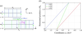


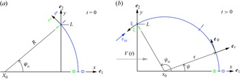


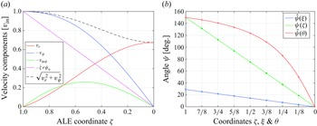


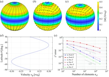


 Open access