


1. Introduction
The focus of this work is on liquid metal flows driven by a strong current passed through the melt, from a thin electrode at one end of the centreline of an axially symmetric vessel, to a wider electrode at the other end. Such flows have been studied extensively, especially with application to material processing and metallurgy (Bojarevičs et al. Reference Bojarevičs, Freibergs, Shilova and Shcherbinin1989; Davidson Reference Davidson1999). Many studies have observed electrovortex flow (EVF) driven by Lorentz forces due to the divergence of the current from the thin electrode (Millere, Sharamkin & Scherbinin Reference Millere, Sharamkin and Scherbinin1980; Bojarevičs et al. Reference Bojarevičs, Millere and Chaikovsky1981; Bojarevičs & Shcherbinin Reference Bojarevičs and Shcherbinin1983; Davidson, He & Lowe Reference Davidson, He and Lowe2000; Weber et al. Reference Weber, Galindo, Priede, Stefani and Weier2015; Herreman et al. Reference Herreman, Nore, Ramos, Cappanera, Guermond and Weber2019; Kolesnichenko et al. Reference Kolesnichenko, Frick, Eltishchev, Mandrykin and Stefani2020; Frick et al. Reference Frick, Mandrykin, Eltishchev and Kolesnichenko2022). When a diverging current interacts with its own magnetic field, the resulting force has non-zero curl and therefore cannot be balanced by pressure, so if no other balancing forces are present, then a flow occurs. The EVF is characterised by an axial jet along the centreline, directed away from the thin electrode (Millere et al. Reference Millere, Sharamkin and Scherbinin1980; Bojarevičs & Shcherbinin Reference Bojarevičs and Shcherbinin1983; Bojarevičs et al. Reference Bojarevičs, Freibergs, Shilova and Shcherbinin1989). In confined domains, the streamlines close around themselves, giving rise to a poloidal flow that finally converges radially back towards the thin electrode from the vessel wall.
Other studies, however, have observed poloidal flow with the same topology as EVF but oriented in the opposite direction, diverging radially away from the thin electrode toward the vessel wall, and later returning towards the thin electrode along the vessel axis. In an early example, Millere et al. (Reference Millere, Sharamkin and Scherbinin1980) observed such motion in a numerical study after introducing a strong axial magnetic field (which they called ‘longitudinal’) to the aforementioned EVF set-up. The authors described this motion as a secondary flow linked to an observed toroidal flow, which they called ‘swirl’. Swirl arises when an axial field interacts with diverging current (Bojarevičs et al. Reference Bojarevičs, Sharamkin and Shcherbinin1977), and Millere et al. (Reference Millere, Sharamkin and Scherbinin1980) found it to be quite fast. Importantly, swirl causes centripetal forces that establish a radial pressure gradient. With swirl localised near the upper boundary, this draws fluid upwards from the bulk and outwards along the upper boundary. In confined domains, streamlines close around themselves, giving rise to a poloidal flow downwards along the sidewalls and returning along the vessel axis (Greenspan Reference Greenspan1968). Millere et al. (Reference Millere, Sharamkin and Scherbinin1980) also observed EVF in the absence of an axial magnetic field, and observed coexisting poloidal vortices (in the meridional plane) in both directions in the presence of an axial magnetic field of intermediate strength.
Bojarevičs & Shcherbinin (Reference Bojarevičs and Shcherbinin1983) noted that swirl was much faster than EVF, not only in the simulations of Millere et al. (Reference Millere, Sharamkin and Scherbinin1980), but also in similar experiments. In a detailed theoretical analysis, they argued that EVF is unstable to toroidal perturbation, and called the resulting transition ‘swirl bifurcation’ because of the (apparently unbounded) growth of swirl velocity. Evidence from experiments in hemispherical geometry with a free surface and a thin electrode (Bojarevičs et al. Reference Bojarevičs, Millere and Chaikovsky1981) seemed consistent with the theory of swirl bifurcation. In contrast, Davidson et al. (Reference Davidson, Kinnear, Lingwood, Short and He1999) gave a different explanation for swirl being faster than EVF. Those authors argued that EVF is not, in fact, unstable; rather, it is suppressed by Ekman pumping. They characterised the competition using the ratio of the typical azimuthal force $F_{{\theta }}$
and the typical poloidal force
$F_{{\theta }}$
and the typical poloidal force $F_{{pol}}$
, finding that EVF was suppressed when
$F_{{pol}}$
, finding that EVF was suppressed when $F_{{\theta }}/F_{{pol}} \sim 0.01$
from numerical simulations utilising the
$F_{{\theta }}/F_{{pol}} \sim 0.01$
from numerical simulations utilising the $k\text{-}\varepsilon$
model. They went on to argue that the low poloidal velocity of EVF allows swirl to dominate. The reasoning echoed an earlier study of flows under swirling magnetic fields (Davidson Reference Davidson1992). The case in which diverging poloidal flow replaces EVF, previously observed by Millere et al. (Reference Millere, Sharamkin and Scherbinin1980), was not considered by Davidson et al. (Reference Davidson, Kinnear, Lingwood, Short and He1999), and was mentioned only briefly, without explanation, by Bojarevičs & Shcherbinin (Reference Bojarevičs and Shcherbinin1983).
$k\text{-}\varepsilon$
model. They went on to argue that the low poloidal velocity of EVF allows swirl to dominate. The reasoning echoed an earlier study of flows under swirling magnetic fields (Davidson Reference Davidson1992). The case in which diverging poloidal flow replaces EVF, previously observed by Millere et al. (Reference Millere, Sharamkin and Scherbinin1980), was not considered by Davidson et al. (Reference Davidson, Kinnear, Lingwood, Short and He1999), and was mentioned only briefly, without explanation, by Bojarevičs & Shcherbinin (Reference Bojarevičs and Shcherbinin1983).
Subsequent studies did observe diverging poloidal flow. Driving flow using rotating and travelling magnetic fields, Grants et al. (Reference Grants, Zhang, Eckert and Gerbeth2008) experimentally observed transition from EVF to diverging poloidal flow when $F_{{\theta }}/F_{{pol}}\sim 0.02$
in a cylindrical geometry. They argued that the transition was marked by formation of a concentrated vortex by swirl accumulation, a process in which a swirling circulation is driven inwards, towards the axis, by a converging poloidal flow, such as EVF. Because the radius of the swirl is reduced, conservation of angular momentum requires that its speed should increase. The result is a small, fast vortex centred near the symmetry axis. Vinogradov, Ivochkin & Teplyakov (Reference Vinogradov, Ivochkin and Teplyakov2018) experimentally investigated the effect of the Earth’s magnetic field (which has an axial component) on EVF dynamics in a hemispherical geometry. They observed the transition between a poloidal-dominated flow to a swirl-dominated flow with poloidal suppression as expected from the analysis by Davidson et al. (Reference Davidson, Kinnear, Lingwood, Short and He1999).
$F_{{\theta }}/F_{{pol}}\sim 0.02$
in a cylindrical geometry. They argued that the transition was marked by formation of a concentrated vortex by swirl accumulation, a process in which a swirling circulation is driven inwards, towards the axis, by a converging poloidal flow, such as EVF. Because the radius of the swirl is reduced, conservation of angular momentum requires that its speed should increase. The result is a small, fast vortex centred near the symmetry axis. Vinogradov, Ivochkin & Teplyakov (Reference Vinogradov, Ivochkin and Teplyakov2018) experimentally investigated the effect of the Earth’s magnetic field (which has an axial component) on EVF dynamics in a hemispherical geometry. They observed the transition between a poloidal-dominated flow to a swirl-dominated flow with poloidal suppression as expected from the analysis by Davidson et al. (Reference Davidson, Kinnear, Lingwood, Short and He1999).
Liquid metal batteries (LMBs) reignited interest in liquid metal flows confined to cylindrical geometries (Weber et al. Reference Weber, Galindo, Priede, Stefani and Weier2015; Kelley & Weier Reference Kelley and Weier2018; Herreman et al. Reference Herreman, Nore, Ramos, Cappanera, Guermond and Weber2019). Numerical simulations by Herreman et al. (Reference Herreman, Nore, Ramos, Cappanera, Guermond and Weber2019) validated the existence of flow structures similar to those observed in hemispherical geometries, namely, a poloidal EVF converging radially towards the thin electrode. Motivated by the effect of flow on mixing and break-up of intermetallics, Herreman et al. (Reference Herreman, Nore, Cappanera and Guermond2021) investigated the scaling of EVF in the presence of an external magnetic field, and found a scaling for swirling EVF in cylinders different from those observed previously in hemispherical geometries.
Kolesnichenko et al. (Reference Kolesnichenko, Frick, Eltishchev, Mandrykin and Stefani2020) were the first to experimentally show poloidal suppression in a cylindrical geometry. Their apparatus had a free surface, and they also showed that as flow develops, EVF arises first, before swirl accumulates enough to cause a secondary flow to suppress it. In a subsequent study, Frick et al. (Reference Frick, Mandrykin, Eltishchev and Kolesnichenko2022) provided experimental confirmation of EVF suppression. They also investigated time-dependent behaviours and the effect of varying the external magnetic field on the flow structure. Like earlier studies in a hemispherical geometry, theirs showed a diverging poloidal flow (in the direction opposite to EVF) in the case of a solid upper boundary and strong external fields. Kharicha et al. (Reference Kharicha, Al-Nasser, Barati, Karimi-Sibaki, Vakhrushev, Abdi, Ludwig and Wu2022) observed flow reversal in a numerical study of EVF with external magnetic field in a cylinder. They analysed different flow morphologies, and found that their transition is controlled by two dimensionless groups.
Taken together, these studies support the idea that when current is passed between a small electrode and a larger one, in a vessel that is either hemispherical or cylindrical, EVF can be suppressed by swirl via Ekman pumping. They further support the idea that the ratio of EVF and Ekman forces should control that suppression, and by extension, transition from EVF to diverging poloidal flow. However, control of transition (as opposed to suppression) has not previously been discussed in detail, and transitions have not been observed at a consistent value of $F_{{\theta }}/F_{{pol}}$
. As we will argue below, recent literature contains insights into the forces and fluid velocities that govern EVF and diverging poloidal flow that have not been taken into account when considering the force balance that leads to transition. In this work, we investigate the transition with a combination of theoretical arguments and novel laboratory experiments. In laboratory experiments, we observed three flow regimes: one with flow converging radially towards the thin electrode, another with flow diverging radially away from the thin electrode, and another where both behaviours appear to compete. We argue that these flows correspond to EVF, swirl-driven Ekman pumping, and a novel observation at the cusp of transition between the two. We propose two possible parameters to capture the transition: one based on the Davidson et al. (Reference Davidson, Kinnear, Lingwood, Short and He1999) force ratio, but incorporating the electrode radius and assuming the local dynamics in the vicinity of the wire electrode control the dynamics, and another where we assume that the global parameters and viscous effects govern the fluid behaviour in the bulk. Using data from this and previous experimental studies on this topic, we argue that both scaling parameters could potentially resolve inconsistencies among prior studies of this topic.
$F_{{\theta }}/F_{{pol}}$
. As we will argue below, recent literature contains insights into the forces and fluid velocities that govern EVF and diverging poloidal flow that have not been taken into account when considering the force balance that leads to transition. In this work, we investigate the transition with a combination of theoretical arguments and novel laboratory experiments. In laboratory experiments, we observed three flow regimes: one with flow converging radially towards the thin electrode, another with flow diverging radially away from the thin electrode, and another where both behaviours appear to compete. We argue that these flows correspond to EVF, swirl-driven Ekman pumping, and a novel observation at the cusp of transition between the two. We propose two possible parameters to capture the transition: one based on the Davidson et al. (Reference Davidson, Kinnear, Lingwood, Short and He1999) force ratio, but incorporating the electrode radius and assuming the local dynamics in the vicinity of the wire electrode control the dynamics, and another where we assume that the global parameters and viscous effects govern the fluid behaviour in the bulk. Using data from this and previous experimental studies on this topic, we argue that both scaling parameters could potentially resolve inconsistencies among prior studies of this topic.
2. Methods
Experiments were carried out using a laboratory LMB model described previously (Cheng et al. Reference Cheng, Mohammad, Wang, Forer and Kelley2022a
), in which boundary temperatures and electrical currents can be controlled, as shown in figure 1(a). The working fluid was liquid gallium maintained at mean temperature 43 $^{\circ }$
C, with density
$^{\circ }$
C, with density $\rho = 5870\,\rm kg\,m^{-3}$
, kinematic viscosity
$\rho = 5870\,\rm kg\,m^{-3}$
, kinematic viscosity $\nu = 2.6\times 10^{-7}\,\rm m^{2}\,s^{-1}$
, thermal diffusivity
$\nu = 2.6\times 10^{-7}\,\rm m^{2}\,s^{-1}$
, thermal diffusivity $\kappa = 1.3 \times 10^{-5}\,\rm m^{2}\,s^{-1}$
, thermal expansion coefficient
$\kappa = 1.3 \times 10^{-5}\,\rm m^{2}\,s^{-1}$
, thermal expansion coefficient $\alpha = 1.25\times 10^{-4}\,\rm K^{-1}$
, and electrical conductivity
$\alpha = 1.25\times 10^{-4}\,\rm K^{-1}$
, and electrical conductivity $\sigma = 3.5\times 10^6\,\rm S\,m^{-1}$
. The Prandtl number (
$\sigma = 3.5\times 10^6\,\rm S\,m^{-1}$
. The Prandtl number ( $Pr$
) was
$Pr$
) was $Pr = 0.02$
. The gallium filled a cylindrical vessel of height
$Pr = 0.02$
. The gallium filled a cylindrical vessel of height $H = 5.0\,\rm cm$
and radius
$H = 5.0\,\rm cm$
and radius $R = 5.0\,\rm cm$
. We fixed the temperatures of the lower and upper plates at 42.9
$R = 5.0\,\rm cm$
. We fixed the temperatures of the lower and upper plates at 42.9 $^{\circ }$
C and 43.1
$^{\circ }$
C and 43.1 $^{\circ }$
C, respectively, with the bottom kept slightly cooler than the top to suppress thermal convection. For both the lower and upper plates, temperature variation across the plate was less than 0.3
$^{\circ }$
C, respectively, with the bottom kept slightly cooler than the top to suppress thermal convection. For both the lower and upper plates, temperature variation across the plate was less than 0.3 $^{\circ }$
C, as monitored by four K-type thermocouples embedded in each copper plate, and an additional thermocouple on the top electrode.
$^{\circ }$
C, as monitored by four K-type thermocouples embedded in each copper plate, and an additional thermocouple on the top electrode.
Current entered the gallium through the lower plate, which served as the positive electrode. Current exited the gallium through a wire of radius $r_w = 3.18\,\rm mm$
at the centre of the upper plate. The wire was electrically insulated from the plate, forcing the current to converge as it passed through the gallium. We performed experiments with current values
$r_w = 3.18\,\rm mm$
at the centre of the upper plate. The wire was electrically insulated from the plate, forcing the current to converge as it passed through the gallium. We performed experiments with current values $I = 5$
, 10, 20, 40, 60 and 80 A for one hour in each case after temperatures had reached a steady state. The value of the electrovortex parameter
$I = 5$
, 10, 20, 40, 60 and 80 A for one hour in each case after temperatures had reached a steady state. The value of the electrovortex parameter $S=\mu _0I^2/(4\unicode{x03C0} ^2 \rho \nu ^2)$
, which characterises the ratio of Lorentz to viscous forces (Bojarevičs et al. Reference Bojarevičs, Freibergs, Shilova and Shcherbinin1989), ranged between
$S=\mu _0I^2/(4\unicode{x03C0} ^2 \rho \nu ^2)$
, which characterises the ratio of Lorentz to viscous forces (Bojarevičs et al. Reference Bojarevičs, Freibergs, Shilova and Shcherbinin1989), ranged between $611$
and
$611$
and $1.57\times 10^5$
.
$1.57\times 10^5$
.
Velocities were measured with ultrasound probes and a DOP3010 velocimeter (Signal Processing, Switzerland). Each probe measures along its line of sight, detecting only the velocity component along that line, as shown in figure 1. The measurements described below came from a subset of the nine ultrasound probes used during experiments.
(a) Schematic of our apparatus. The velocity field is illustrative, courtesy of Personnettaz et al. (Reference Personnettaz, Landgraf, Nimtz, Weber and Weier2019). (b) Positions and orientations of probes 3, 4, 8 and 9. Probes 3 and 4 were placed radially and perpendicular to each other at height $3H/4 = 3.75\,\rm cm$
from the bottom. Probes 8 and 9 were oriented vertically over the beam of probe 3, with probe 8 located
$3H/4 = 3.75\,\rm cm$
from the bottom. Probes 8 and 9 were oriented vertically over the beam of probe 3, with probe 8 located $4\,\rm mm$
from the wall, and probe 9 located
$4\,\rm mm$
from the wall, and probe 9 located $12.5\,\rm mm$
from the centreline. (c) Positions and orientations of probes 5, 6 and 7 (view is rotated
$12.5\,\rm mm$
from the centreline. (c) Positions and orientations of probes 5, 6 and 7 (view is rotated $180^{\circ }$
from that in (b)). These are placed in chord positions anti-parallel to probe 3 and offset
$180^{\circ }$
from that in (b)). These are placed in chord positions anti-parallel to probe 3 and offset $R/2 = 2.5\,\rm cm$
to either side. Probe 5 was at height
$R/2 = 2.5\,\rm cm$
to either side. Probe 5 was at height $H/2$
, probe 6 was at height
$H/2$
, probe 6 was at height $3H/4$
, and probe 7 was at height
$3H/4$
, and probe 7 was at height $H/4$
.
$H/4$
.

3. Results
Velocity measurements from an experiment with a strong (80 A) current are shown in figure 2. Probe 9 detected flow away from itself, indicating downward flow near the vessel centreline. Probe 8 detected flow towards itself, indicating upward flow near the vessel edge. Probes 3 and 4 both measured flow consistently away from themselves for $x \lt 40\,\rm mm$
, and towards themselves for
$x \lt 40\,\rm mm$
, and towards themselves for $x \gt 55\,\rm mm$
. (A narrow region of fast flow towards probe 3 near the vessel centreline was also detected and will be discussed below.) Taken together, these measurements are consistent with a global, poloidal circulation in which fluid rose near vessel edges, converged towards the thin electrode at the centreline, and descended in a jet away from it, as sketched in figure 2(f). This is the circulation expected from EVF when the thin electrode is at the top of the vessel centreline, as in our apparatus.
$x \gt 55\,\rm mm$
. (A narrow region of fast flow towards probe 3 near the vessel centreline was also detected and will be discussed below.) Taken together, these measurements are consistent with a global, poloidal circulation in which fluid rose near vessel edges, converged towards the thin electrode at the centreline, and descended in a jet away from it, as sketched in figure 2(f). This is the circulation expected from EVF when the thin electrode is at the top of the vessel centreline, as in our apparatus.
Typical flow with a strong current. (a–d) Velocities varying over time $t$
and distance
$t$
and distance $x$
from each probe (in each probe’s own frame of reference), measured while running an 80 A current. Blue indicates flow towards the probe; red indicates flow away from it. (e) Time-averaged velocities, with numerals at probe positions. (f) A sketch of the apparent flow structure, in which fluid converges radially towards the thin electrode and descends near the vessel centreline, and a fast horizontal swirl occurs near the top of the centreline.
$x$
from each probe (in each probe’s own frame of reference), measured while running an 80 A current. Blue indicates flow towards the probe; red indicates flow away from it. (e) Time-averaged velocities, with numerals at probe positions. (f) A sketch of the apparent flow structure, in which fluid converges radially towards the thin electrode and descends near the vessel centreline, and a fast horizontal swirl occurs near the top of the centreline.

We observed different flows in experiments with weak current; one example is the 20 A case shown in figure 3. At this current value, fluid rose near the vessel centreline, moving towards probe 9, and descended near the vessel edge, away from probe 8. The flow diverged horizontally near the top, as detected by probes 3 and 4, which found motion towards themselves for $x \lt 40\,\rm mm$
, and away from themselves for
$x \lt 40\,\rm mm$
, and away from themselves for $x \gt 55\,\rm mm$
. (Discussion of the narrow region of fast flow near the vessel centreline is again deferred.) Measurements were consistent with a poloidal circulation that diverged radially from the thin electrode, as sketched in figure 3(f), and suggested that EVF had been suppressed and overcome by opposing forces.
$x \gt 55\,\rm mm$
. (Discussion of the narrow region of fast flow near the vessel centreline is again deferred.) Measurements were consistent with a poloidal circulation that diverged radially from the thin electrode, as sketched in figure 3(f), and suggested that EVF had been suppressed and overcome by opposing forces.
Typical flow with a weak current. (a–d) Velocities measured while running a 20 A current, plotted as in figure 2. (e) Time-averaged velocity measurements. (f) A sketch of the apparent flow structure, in which fluid diverges radially from the thin electrode and rises near the vessel centreline.

Whereas the probes considered in figures 2 and 3 were placed to detect poloidal motions, probes 5, 6 and 7 were placed for detecting swirl, oriented horizontally and positioned away from the centreline. Measurements from those probes are shown in figure 4. In experiments with weak current, our observations were consistent with a global clockwise circulation, throughout space and time. When current was weak, toroidal flow was always faster than poloidal flow, indicating that swirl dominated. In experiments with strong current, probes 5, 6 and 7 detected more complicated flow patterns, though clockwise circulation seems to have persisted in at least part of the vessel.
Typical large-scale swirl flow, varying with current. In experiments with currents up to 40 A, fluid flows away from probe 5 and towards probes 6 and 7, suggesting a global, azimuthal circulation in the clockwise direction (as seen from above). With stronger currents, the flow pattern is more complicated.

The narrow region of fast flow detected near the vessel centreline by probes 3 and 4, mentioned above, is also consistent with clockwise circulation. Though a purely toroidal swirl flow would have no velocity in the radial direction, and would therefore be undetectable by probes 3 and 4, a swirl flow slightly offset from the centreline, towards probe 3 in all cases, and towards probe 4 for weak currents, would lead to measurements like those shown in figures 2 and 3. In fact, previous work on magnetically driven swirl flows observed a similar offset (Grants et al. Reference Grants, Zhang, Eckert and Gerbeth2008), and previous work on EVF showed a slight deformation or ‘pinching’ of the free surface near the electrode (Kharicha et al. Reference Kharicha, Teplyakov, Ivochkin, Wu, Ludwig and Guseva2015), which would displace the swirl. Apparently, slight asymmetries in our apparatus, such as the placement of probes, cause a consistent offset. This is unsurprising given that previous studies using the same apparatus to study thermal convection found a preferred orientation of the large-scale circulation (Cheng et al. Reference Cheng, Mohammad, Wang, Keogh, Forer and Kelley2022b ).
Clockwise circulation is consistent with our expectations for swirl driven by interaction between the current, which converges radially, and the vertical component of Earth’s magnetic field, which points downwards in our laboratory. Our observations that flow is fastest in the narrow region near the vessel centreline can be explained by the fact that the current density is highest there. Fast swirl in the narrow region might also be amplified by swirl accumulation when EVF drives a poloidal motion that converges towards the thin electrode, sweeping toroidal circulation inwards (Grants et al. Reference Grants, Zhang, Eckert and Gerbeth2008), but not when a diverging poloidal flow occurs. The fact that flow is fastest in the region near the narrow electrode suggests that the electrode radius is an important characteristic scale, as will be discussed below.
As has been noted previously (Davidson et al. Reference Davidson, Kinnear, Lingwood, Short and He1999; Herreman et al. Reference Herreman, Nore, Cappanera and Guermond2021), swirl can induce Ekman pumping that drives flow outwards at the upper boundary, downwards along the sidewalls, and upwards along the centreline. Such a diverging poloidal flow is consistent with the velocities that we observed when the current was weak, and consistent with previous observations (e.g. Millere et al. Reference Millere, Sharamkin and Scherbinin1980; Frick et al. Reference Frick, Mandrykin, Eltishchev and Kolesnichenko2022; Kharicha et al. Reference Kharicha, Al-Nasser, Barati, Karimi-Sibaki, Vakhrushev, Abdi, Ludwig and Wu2022). We argue that swirl-induced Ekman pumping is the mechanism that gave rise to diverging poloidal flows in our experiments.
Circulations in opposite directions for strong and weak currents imply a transition at intermediate current. While flows in both directions have been observed previously, we believe that the velocity measurements shown in figure 5 at 40 A current are the first to visualise a transition case where swirl-induced Ekman pumping and EVF are competing and alternating in time. Probes 8 and 9 detected weak spatial variation in the flow; at any given moment, the measured velocity was typically uniformly positive or negative. However, both probes detected temporal variation, with the direction reversing often and erratically. Similarly, probes 3 and 4 detected, for $x \lt 40\,\rm mm$
and
$x \lt 40\,\rm mm$
and $x \gt 55\,\rm mm$
, frequent and erratic changes from converging to diverging horizontal flow. Though unpredictable, changes tended to occur simultaneously in all four probes.
$x \gt 55\,\rm mm$
, frequent and erratic changes from converging to diverging horizontal flow. Though unpredictable, changes tended to occur simultaneously in all four probes.
Typical flow with moderate current. Velocities measured while running a 40 A current, plotted as in figure 2. The measurements suggest an alternation between EVF, observed with strong currents, and swirl-induced Ekman pumping, observed with weak currents. The dashed lines indicate a strong local swirl near the electrode indicated in figures 2(f) and 3(f).

On the other hand, the fast flow near the top of the centreline, detected by probes 3 and 4, tended to maintain the same direction throughout time and regardless of the magnitude of the current, as shown in figures 2, 3, 4 and 5. That observation matches our expectations for a local horizontal swirl, since neither the current nor Earth’s magnetic field changed direction. There is only one exception: probe 4 measured no central fast flow at all in the 80 A experiment (figure 2 d). We believe that the local swirl flow migrated slightly, such that it either aligned with the centreline or moved entirely out of the line of sight of probe 4.
We look further into the variation of velocity with current by comparing measurements with the swirl flow scaling proposed by Herreman et al. (Reference Herreman, Nore, Cappanera and Guermond2021):
 \begin{equation} U_{\textit{swirl}} \sim \left (\dfrac {JB_{\textit{ext}}}{\rho }\right )^{2/3}\left (\dfrac {R}{\nu ^{1/3}}\right ). \end{equation}
Here, $U_{\textit{swirl}}$
is the characteristic speed,
$U_{\textit{swirl}}$
is the characteristic speed, $J=I \unicode{x03C0} ^{-1} R^{-2}$
is the current density, and
$J=I \unicode{x03C0} ^{-1} R^{-2}$
is the current density, and $B_{\textit{ext}}$
is the vertical component of the external magnetic field. Our measurements can also be compared to the EVF scaling proposed by Bojarevičs et al. (Reference Bojarevičs, Freibergs, Shilova and Shcherbinin1989):
$B_{\textit{ext}}$
is the vertical component of the external magnetic field. Our measurements can also be compared to the EVF scaling proposed by Bojarevičs et al. (Reference Bojarevičs, Freibergs, Shilova and Shcherbinin1989):
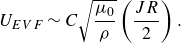 \begin{equation} U_{{EVF}} \sim C\sqrt {\dfrac {\mu _0}{\rho }} \left (\dfrac {JR}{2}\right ). \end{equation}
Here, $U_{{EVF}}$
is the characteristic speed,
$U_{{EVF}}$
is the characteristic speed, $\mu _0$
is the permittivity of free space, and
$\mu _0$
is the permittivity of free space, and $C=(10^{3-5\Gamma })^{1/3}$
, where
$C=(10^{3-5\Gamma })^{1/3}$
, where $\Gamma =r_{{w}}/R$
. Both
$\Gamma =r_{{w}}/R$
. Both $U_{{swirl}}$
and
$U_{{swirl}}$
and $U_{{EVF}}$
depend on
$U_{{EVF}}$
depend on $J$
(and therefore
$J$
(and therefore $I$
), going to zero when there is no current, and increasing monotonically as current increases. Importantly, (3.1) and (3.2) imply that
$I$
), going to zero when there is no current, and increasing monotonically as current increases. Importantly, (3.1) and (3.2) imply that $U_{{swirl}}(J) = U_{{EVF}}(J)$
at just one non-zero value of
$U_{{swirl}}(J) = U_{{EVF}}(J)$
at just one non-zero value of $J$
. For
$J$
. For $J \rightarrow 0$
,
$J \rightarrow 0$
, $J^{2/3} \gt J^1$
and therefore
$J^{2/3} \gt J^1$
and therefore $U_{{swirl}} \gt U_{{EVF}}$
, but for
$U_{{swirl}} \gt U_{{EVF}}$
, but for $J \rightarrow \infty$
,
$J \rightarrow \infty$
, $J^1 \gt J^{2/3}$
and therefore
$J^1 \gt J^{2/3}$
and therefore $U_{{EVF}} \gt U_{{swirl}}$
. These relationships are consistent with our observations that Ekman pumping dominates when current is weak, and EVF dominates when current is strong.
$U_{{EVF}} \gt U_{{swirl}}$
. These relationships are consistent with our observations that Ekman pumping dominates when current is weak, and EVF dominates when current is strong.
To learn more about how speed varies with current, we consider time-averaged velocities from experiments with varying current magnitudes, shown in figure 6. We averaged over the total duration of each experiment ( 58–62 minutes, with 1700–1800 measurements per probe). With weak currents (5 A, 10 A, 20 A), the measurements indicate flow diverging radially from the thin electrode. For strong currents (60 A, 80 A), they indicate flow in the opposite direction. For the transitional case (40 A), the time-averaged vertical velocity is near zero in both locations, though the instantaneous vertical velocity is not (see figure 5). All those facts are again consistent with two poloidal flows, one that diverges from the thin electrode with weak currents, and another that converges towards the thin electrode with strong currents, suggesting a transition from swirl-induced Ekman pumping to EVF.
Importantly, figure 6 illustrates variations not only of flow direction but also of speed. When the current is low and the flow direction is that of swirl-induced Ekman pumping, its speed varies only weakly with current. In contrast, when the current is strong and the flow direction is that of EVF, its speed varies strongly with current. Finding greater sensitivity with strong currents matches our expectations from the scaling relationships, since $U_{{EVF}} \sim J^1$
, predicted to dominate when
$U_{{EVF}} \sim J^1$
, predicted to dominate when $J \rightarrow \infty$
, depends more strongly on
$J \rightarrow \infty$
, depends more strongly on $J$
than does
$J$
than does $U_{{swirl}} \sim J^{2/3}$
, predicted to dominate when
$U_{{swirl}} \sim J^{2/3}$
, predicted to dominate when $J \rightarrow 0$
. These observations further support the idea that our experiments were dominated by EVF with strong currents, and swirl-induced Ekman pumping with weak currents.
$J \rightarrow 0$
. These observations further support the idea that our experiments were dominated by EVF with strong currents, and swirl-induced Ekman pumping with weak currents.
Time-averaged velocity $\overline {V}$
plotted versus current and distance
$\overline {V}$
plotted versus current and distance $x$
from each of probes 8 (continuous curves) and 9 (dotted curves). Shaded regions represent the uncertainty in velocity measurements derived from the probe resolution. In (b), the resolution is small enough compared to the velocity magnitude that the shaded regions are not visible. With strong currents: (b) velocities had greater magnitude than with weak currents; (a) had opposite sign, and depended more sensitively on current. In the transitional case when the current was 40 A, though the instantaneous speed was often large (see figure 5), frequent reversals meant
$x$
from each of probes 8 (continuous curves) and 9 (dotted curves). Shaded regions represent the uncertainty in velocity measurements derived from the probe resolution. In (b), the resolution is small enough compared to the velocity magnitude that the shaded regions are not visible. With strong currents: (b) velocities had greater magnitude than with weak currents; (a) had opposite sign, and depended more sensitively on current. In the transitional case when the current was 40 A, though the instantaneous speed was often large (see figure 5), frequent reversals meant $\overline {V} \approx 0$
.
$\overline {V} \approx 0$
.

Figure 7 further quantifies the variation of speed with current. To characterise the fast motion near the wire, we used $\overline {V}_{{peak}}$
, defined as the maximum value of the time-averaged speed, for probes 3 and 4. We chose the peak value because swirl flow is faster than other observed features, and it apparently moves in and out of the lines of sight of the probes. To characterise speeds measured by the horizontal chord probes 5–7, which were positioned lower than probes 3 and 4, and sampled bulk toroidal motion, we used the median speed over both space and time,
$\overline {V}_{{peak}}$
, defined as the maximum value of the time-averaged speed, for probes 3 and 4. We chose the peak value because swirl flow is faster than other observed features, and it apparently moves in and out of the lines of sight of the probes. To characterise speeds measured by the horizontal chord probes 5–7, which were positioned lower than probes 3 and 4, and sampled bulk toroidal motion, we used the median speed over both space and time, $V_{{ma}}$
. These measurements show that flow speed appears more sensitive to current variations for strong currents than for weak currents, as we would expect in a transition from Ekman pumping to EVF in which their characteristic speeds are, at least approximately, consistent with (3.1) and (3.2). That said, the scaling laws do not correspond to precise velocity predictions, and are further complicated by the one-dimensional nature of our measurements. Scatter in the measurements shown in figure 7 suggests that the observed flows may be more complex than (3.1) and (3.2) can capture. Neither the
$V_{{ma}}$
. These measurements show that flow speed appears more sensitive to current variations for strong currents than for weak currents, as we would expect in a transition from Ekman pumping to EVF in which their characteristic speeds are, at least approximately, consistent with (3.1) and (3.2). That said, the scaling laws do not correspond to precise velocity predictions, and are further complicated by the one-dimensional nature of our measurements. Scatter in the measurements shown in figure 7 suggests that the observed flows may be more complex than (3.1) and (3.2) can capture. Neither the $I=5$
A case for probe 3 nor the
$I=5$
A case for probe 3 nor the $I=80$
A case for probe 4 is plotted in figure 7 because no fast, local circulation was detected in either case. That is, the flow pattern indicative of fast, small swirl near the top centre, like the narrow high-speed region near
$I=80$
A case for probe 4 is plotted in figure 7 because no fast, local circulation was detected in either case. That is, the flow pattern indicative of fast, small swirl near the top centre, like the narrow high-speed region near $x=40\,\rm mm$
in figure 2(c), did not appear. As discussed earlier, we believe that such a swirl was present but located where probes 3 and 4 could not detect it.
$x=40\,\rm mm$
in figure 2(c), did not appear. As discussed earlier, we believe that such a swirl was present but located where probes 3 and 4 could not detect it.
Velocity scaling and flow transition. (a) Peak time-averaged velocity $\overline {V}_{{peak}}$
measured by probes 3 and 4, which characterises the speed of the local swirl near the thin electrode at the upper plate. (b) Median speed
$\overline {V}_{{peak}}$
measured by probes 3 and 4, which characterises the speed of the local swirl near the thin electrode at the upper plate. (b) Median speed $V_{{ma}}$
measured by probes 5–7, which characterises global swirl. Lines show the trends predicted by (3.1) and (3.2), which are not inconsistent with the measurements. Error bars in (a) indicate standard error of the mean. Error bars in (b) indicate standard deviation of the median. All error bars were produced by splitting the
$V_{{ma}}$
measured by probes 5–7, which characterises global swirl. Lines show the trends predicted by (3.1) and (3.2), which are not inconsistent with the measurements. Error bars in (a) indicate standard error of the mean. Error bars in (b) indicate standard deviation of the median. All error bars were produced by splitting the ${\sim}60$
-minute recordings into ten equal intervals.
${\sim}60$
-minute recordings into ten equal intervals.

Possible predictors of flow transition. Each open symbol represents an experiment in which flow diverged radially from the thin electrode, consistent with EVF; each filled symbol represents an experiment in which flow converged towards the thin electrode, consistent with swirl-induced Ekman pumping. Our experiments and those of Frick et al. (Reference Frick, Mandrykin, Eltishchev and Kolesnichenko2022) are shown. (a) Here, $\beta _w = 0.02$
(dashed line) successfully separates EVF from swirl flow in both studies. (b) Here,
$\beta _w = 0.02$
(dashed line) successfully separates EVF from swirl flow in both studies. (b) Here, $\lambda _R = 12.4$
is also successful. (c) Here,
$\lambda _R = 12.4$
is also successful. (c) Here, $\beta _R$
cannot separate EVF from swirl flow; any line of constant
$\beta _R$
cannot separate EVF from swirl flow; any line of constant $\beta _R$
puts at least one experiment the wrong side of the line (circled in yellow). (d) Here,
$\beta _R$
puts at least one experiment the wrong side of the line (circled in yellow). (d) Here, $\lambda _w$
is also unsuccessful.
$\lambda _w$
is also unsuccessful.

4. Discussion
4.1. Force balance
We established above that a transition between swirl-induced Ekman pumping and EVF appeared to occur in our experiments, consistent with prior predictions of velocity scaling. This transition may be explained by extending the reasoning used by Davidson et al. (Reference Davidson, Kinnear, Lingwood, Short and He1999), who found that EVF was suppressed when the ratio between the toroidal and poloidal forces reached 0.01. A characteristic toroidal force is
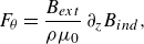 \begin{equation} F_\theta =\dfrac {B_{{ext}}}{\rho \mu _0}\, \partial _z B_{{ind}}, \end{equation}
where $B_{{ext}}$
is the vertical external magnetic field, and
$B_{{ext}}$
is the vertical external magnetic field, and $B_{{ind}}$
is the induced toroidal magnetic field. (Davidson et al. (Reference Davidson, Kinnear, Lingwood, Short and He1999) refer to these quantities as
$B_{{ind}}$
is the induced toroidal magnetic field. (Davidson et al. (Reference Davidson, Kinnear, Lingwood, Short and He1999) refer to these quantities as $B_z$
and
$B_z$
and $B_\theta$
, respectively.) A characteristic poloidal force is
$B_\theta$
, respectively.) A characteristic poloidal force is
 \begin{equation} F_{{pol}} = \dfrac {B_{{ind}}^2}{\rho \mu _0 r}, \end{equation}
where $r$
is a characteristic radius. Note that
$r$
is a characteristic radius. Note that $F_{{pol}}$
as written above omits the magnetic pressure, a term that will not affect the dynamics. Since we would expect
$F_{{pol}}$
as written above omits the magnetic pressure, a term that will not affect the dynamics. Since we would expect $F_\theta$
to be large when swirl-induced Ekman pumping dominates, and
$F_\theta$
to be large when swirl-induced Ekman pumping dominates, and $F_{{pol}}$
to be large when EVF dominates, the force ratio
$F_{{pol}}$
to be large when EVF dominates, the force ratio $F_\theta / F_{{pol}}$
can be translated into a concrete prediction for the transition by choosing values for the characteristic quantities in (4.1) and (4.2).
$F_\theta / F_{{pol}}$
can be translated into a concrete prediction for the transition by choosing values for the characteristic quantities in (4.1) and (4.2).
The chosen values should be compatible with the fact that current density is far from uniform. Liu et al. (Reference Liu, Stefani, Weber, Weier and Li2020) found that current density near the electrode scales with the wire radius $r_{{w}}$
. Bojarevičs & Shcherbinin (Reference Bojarevičs and Shcherbinin1983) noted that the ratio between electrode radii in the hemispherical system affected flow intensity. Frick et al. (Reference Frick, Mandrykin, Eltishchev and Kolesnichenko2022) stressed that poloidal suppression depended on the structure of the current density. Bénard et al. (Reference Bénard, Herreman, Guermond and Nore2022) investigated the effect of the ratio of wire radius to cylinder radius
$r_{{w}}$
. Bojarevičs & Shcherbinin (Reference Bojarevičs and Shcherbinin1983) noted that the ratio between electrode radii in the hemispherical system affected flow intensity. Frick et al. (Reference Frick, Mandrykin, Eltishchev and Kolesnichenko2022) stressed that poloidal suppression depended on the structure of the current density. Bénard et al. (Reference Bénard, Herreman, Guermond and Nore2022) investigated the effect of the ratio of wire radius to cylinder radius $\Gamma =r_{{w}}/R$
, finding a super-linear decay of speed with
$\Gamma =r_{{w}}/R$
, finding a super-linear decay of speed with $\Gamma$
.
$\Gamma$
.
Since current density is highest near the thin electrode, the Lorentz forces that drive EVF must likewise be strongest there. We therefore choose $r=r_w$
when using (4.2) to estimate
$r=r_w$
when using (4.2) to estimate $F_{{pol}}$
. We then scale
$F_{{pol}}$
. We then scale $\partial _z B_{{ind}}$
as
$\partial _z B_{{ind}}$
as $B_{{ind}}/H = B_{{ind}}/R$
(for aspect ratio
$B_{{ind}}/H = B_{{ind}}/R$
(for aspect ratio $D/H=2$
), such that the force ratio scales as
$D/H=2$
), such that the force ratio scales as
 \begin{equation} \frac {\dfrac {B_{{ext}} B_{{ind}}}{\rho \mu _0 R}}{\dfrac {B_{{ind}}^2}{\rho \mu _0 r_w}} = \frac {B_{{ext}}}{B_{{ind}}}\, \Gamma \equiv \beta _w \, . \end{equation}
If the transition that we observe is an extension of the EVF suppression explained by Davidson et al. (Reference Davidson, Kinnear, Lingwood, Short and He1999), then we would expect to observe swirl-induced Ekman pumping when $\beta _w$
exceeds some critical value near 0.01, and we would expect to observe EVF when
$\beta _w$
exceeds some critical value near 0.01, and we would expect to observe EVF when $\beta _w$
falls short of that value.
$\beta _w$
falls short of that value.
Those expectations apply not only to our experiments but to the recent experiments of Frick et al. (Reference Frick, Mandrykin, Eltishchev and Kolesnichenko2022). Their vessel, like ours, was a cylinder with a vertical axis and converging current, although they also incorporated electromagnets that allowed control of $B_{{ext}}$
. Frick et al. (Reference Frick, Mandrykin, Eltishchev and Kolesnichenko2022) performed experiments in two parts. In part I, they varied
$B_{{ext}}$
. Frick et al. (Reference Frick, Mandrykin, Eltishchev and Kolesnichenko2022) performed experiments in two parts. In part I, they varied $I$
(and therefore
$I$
(and therefore $B_{{ind}}$
) while holding
$B_{{ind}}$
) while holding $B_{{ext}}$
constant (as we did). In part II, they varied
$B_{{ext}}$
constant (as we did). In part II, they varied $B_{{ext}}$
while holding
$B_{{ext}}$
while holding $I$
constant. Though the mean poloidal flows never changed direction in part I, they did in part II. This demonstrates that transition can be caused by variations in either
$I$
constant. Though the mean poloidal flows never changed direction in part I, they did in part II. This demonstrates that transition can be caused by variations in either $B_{{ext}}$
or
$B_{{ext}}$
or $B_{{ind}}$
.
$B_{{ind}}$
.
Figure 8(a) demonstrates that in our experimental results and those of Frick et al. (Reference Frick, Mandrykin, Eltishchev and Kolesnichenko2022), swirl-induced Ekman pumping was observed in experiments for which $\beta _w \gt 0.02$
, and EVF was observed in experiments for which
$\beta _w \gt 0.02$
, and EVF was observed in experiments for which $\beta _w \lt 0.02$
. The experiment in which we observed intermittent competition had
$\beta _w \lt 0.02$
. The experiment in which we observed intermittent competition had $\beta _w = 0.02$
. (These statements apply to the available experiments, for which
$\beta _w = 0.02$
. (These statements apply to the available experiments, for which $\beta _w$
ranged from
$\beta _w$
ranged from $0.0007$
to
$0.0007$
to $0.3750$
.) This critical value is also consistent with the transition found in Grants et al. (Reference Grants, Zhang, Eckert and Gerbeth2008), and close to the 0.01 discussed by Davidson et al. (Reference Davidson, Kinnear, Lingwood, Short and He1999) for hemispherical (as opposed to cylindrical) vessels. Thus
$0.3750$
.) This critical value is also consistent with the transition found in Grants et al. (Reference Grants, Zhang, Eckert and Gerbeth2008), and close to the 0.01 discussed by Davidson et al. (Reference Davidson, Kinnear, Lingwood, Short and He1999) for hemispherical (as opposed to cylindrical) vessels. Thus $\beta _w$
seems to accurately predict whether swirl-induced Ekman pumping or EVF will dominate. We note that
$\beta _w$
seems to accurately predict whether swirl-induced Ekman pumping or EVF will dominate. We note that $\beta _w$
can also be expressed in terms of established dimensionless variables:
$\beta _w$
can also be expressed in terms of established dimensionless variables:
 \begin{equation} \beta _w=\frac {Ha\, \Gamma }{\sqrt {Pm\,S}}, \end{equation}
where $Pm = \nu \mu _0 \sigma _0$
is the magnetic Prandtl number,
$Pm = \nu \mu _0 \sigma _0$
is the magnetic Prandtl number, $\sigma _0$
is the conductivity,
$\sigma _0$
is the conductivity, $S = \mu _0 I^2 / (4\unicode{x03C0} ^2 \rho \nu ^2)$
, and
$S = \mu _0 I^2 / (4\unicode{x03C0} ^2 \rho \nu ^2)$
, and $Ha = BR(\sigma \nu )^{1/2}$
is the Hartmann number. The inclusion of
$Ha = BR(\sigma \nu )^{1/2}$
is the Hartmann number. The inclusion of $\Gamma$
is essential to predict the transition.
$\Gamma$
is essential to predict the transition.
4.2. Velocity balance
Alternatively, it seems intuitive to predict the transition from the ratio of characteristic velocities in the bulk: the transition may occur when the EVF velocity reaches a certain fraction of the swirl-induced poloidal velocity. The ratio is
 \begin{equation} \dfrac {U_{{swirl}}}{U_{{EVF}}}= \dfrac {2^{2/3}B_{{ext}}^{2/3}}{B_{{ind}}^{1/3}}\left (\dfrac {R^2}{\mu _0\rho \nu ^2}\right )^{1/6} , \end{equation}
where we have used (3.1) and (3.2) to estimate velocities, and used the approximation $J=2B_{{ind}}/\mu _0 R$
. If we raise the expression to the
$J=2B_{{ind}}/\mu _0 R$
. If we raise the expression to the $3/2$
power, then it becomes
$3/2$
power, then it becomes
 \begin{equation} \dfrac {2 B_{{ext}}}{\sqrt {B_{{ind}}}\left (\dfrac {\mu _0\rho \nu ^2}{R^2}\right )^{1/4}} \equiv \lambda _R . \end{equation}
Unlike $\beta _w$
,
$\beta _w$
, $\lambda _R$
takes the characteristic radius to be the vessel radius
$\lambda _R$
takes the characteristic radius to be the vessel radius $R$
, not the wire radius
$R$
, not the wire radius $r_w$
. Accordingly,
$r_w$
. Accordingly, $\lambda _R$
can be interpreted as involving global, not local, velocities.
$\lambda _R$
can be interpreted as involving global, not local, velocities.
Figure 8(b) shows that $\lambda _R$
, like
$\lambda _R$
, like $\beta _w$
, appears to predict whether EVF or swirl-induced Ekman pumping will dominate in an experiment. For our transition case,
$\beta _w$
, appears to predict whether EVF or swirl-induced Ekman pumping will dominate in an experiment. For our transition case, $\lambda _R = 12.4$
. Swirl-induced Ekman pumping was observed when
$\lambda _R = 12.4$
. Swirl-induced Ekman pumping was observed when $\lambda _R \gt 12.4$
, and EVF was observed when
$\lambda _R \gt 12.4$
, and EVF was observed when $\lambda _R \lt 12.4$
. (These statements apply to the available experiments, for which
$\lambda _R \lt 12.4$
. (These statements apply to the available experiments, for which $\lambda _R$
ranged from
$\lambda _R$
ranged from $2.334$
to
$2.334$
to $398.553$
.) We also note that the transition captured by the velocity ratio happens at
$398.553$
.) We also note that the transition captured by the velocity ratio happens at $\lambda _R^{2/3}\sim 1$
. Importantly, the velocity scaling of Herreman et al. (Reference Herreman, Nore, Cappanera and Guermond2021) in (3.1) accounts for viscous dissipation in the boundary layer; it is derived from a triple balance between the Lorentz, inertial and viscous terms in the vorticity equation. As noted in Davidson (Reference Davidson1992) and Davidson et al. (Reference Davidson, Kinnear, Lingwood, Short and He1999), the boundary controls the dynamics of the Ekman pumping mechanism.
$\lambda _R^{2/3}\sim 1$
. Importantly, the velocity scaling of Herreman et al. (Reference Herreman, Nore, Cappanera and Guermond2021) in (3.1) accounts for viscous dissipation in the boundary layer; it is derived from a triple balance between the Lorentz, inertial and viscous terms in the vorticity equation. As noted in Davidson (Reference Davidson1992) and Davidson et al. (Reference Davidson, Kinnear, Lingwood, Short and He1999), the boundary controls the dynamics of the Ekman pumping mechanism.
4.3. Alternative but unsuccessful formulations
An alternative force balance can be considered. As noted above, $\beta _w$
is the ratio of local characteristic forces near the electrode. What happens if we instead construct a ratio of global characteristic forces throughout the vessel? If we choose
$\beta _w$
is the ratio of local characteristic forces near the electrode. What happens if we instead construct a ratio of global characteristic forces throughout the vessel? If we choose $r = R$
(instead of
$r = R$
(instead of $r = r_w$
) when using (4.2) to estimate
$r = r_w$
) when using (4.2) to estimate $F_{{pol}}$
, then the force ratio scales as
$F_{{pol}}$
, then the force ratio scales as
 \begin{equation} \dfrac {\dfrac {B_{{ext}} B_{{ind}}}{\rho \mu _0 R}}{\dfrac {B_{{ind}}^2}{\rho \mu _0 R}} = \dfrac {B_{{ext}}}{B_{{ind}}} \equiv \beta _R . \end{equation}
The experiment in which we observed intermittent competition had $\beta _R = 0.3$
. However, as figure 8(c) demonstrates, of the experiments in which apparent swirl-induced Ekman pumping was observed, most have
$\beta _R = 0.3$
. However, as figure 8(c) demonstrates, of the experiments in which apparent swirl-induced Ekman pumping was observed, most have $\beta _R \gt 0.3$
, but one has
$\beta _R \gt 0.3$
, but one has $\beta _R \lt 0.3$
. This result is not particular to the value
$\beta _R \lt 0.3$
. This result is not particular to the value $\beta _R = 0.3$
; no line of constant
$\beta _R = 0.3$
; no line of constant $\beta _R$
accurately separates swirl-induced Ekman pumping from EVF.
$\beta _R$
accurately separates swirl-induced Ekman pumping from EVF.
An alternative velocity balance can also be considered. In constructing $\lambda _R$
, we scaled the current density in (3.1) and (3.2) with the vessel radius
$\lambda _R$
, we scaled the current density in (3.1) and (3.2) with the vessel radius $R$
. If the current is highly concentrated near the electrode, however, then it can be argued that scaling the current density with
$R$
. If the current is highly concentrated near the electrode, however, then it can be argued that scaling the current density with $r_w$
makes more sense. In doing so, the ratio between
$r_w$
makes more sense. In doing so, the ratio between $U_{{swirl}}$
and
$U_{{swirl}}$
and $U_{{EVF}}$
is
$U_{{EVF}}$
is
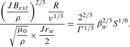 \begin{equation} \dfrac {\left ( \dfrac {J B_{{ext}}}{\rho } \right )^{2/3} \dfrac {R}{\nu ^{1/3}}}{\sqrt {\dfrac {\mu _0}{\rho }} \times \dfrac {J r_w}{2}} = \frac {2^{2/3}}{\Gamma ^{1/3}}\,\beta _w^{2/3}S^{1/6}. \end{equation}
If we again raise the resulting expression to the $3/2$
power, then it becomes
$3/2$
power, then it becomes
 \begin{equation} \hat {C}\beta _w S^{1/4} \equiv \lambda _w \, , \end{equation}
where $\hat {C}=\sqrt {\Gamma \times 10^{3-5\Gamma }}/2$
. The experiment in which we observed intermittent competition had
$\hat {C}=\sqrt {\Gamma \times 10^{3-5\Gamma }}/2$
. The experiment in which we observed intermittent competition had $\lambda _w = 0.15$
. However, as figure 8(d) demonstrates, of the experiments in which apparent EVF was observed, most have
$\lambda _w = 0.15$
. However, as figure 8(d) demonstrates, of the experiments in which apparent EVF was observed, most have $\lambda _w \lt 0.15$
, but two have
$\lambda _w \lt 0.15$
, but two have $\lambda _w \gt 0.15$
. This result is not particular to the value
$\lambda _w \gt 0.15$
. This result is not particular to the value $\lambda _w = 0.15$
; no line of constant
$\lambda _w = 0.15$
; no line of constant $\lambda _w$
accurately separates Ekman pumping from EVF.
$\lambda _w$
accurately separates Ekman pumping from EVF.
4.4. Summary and caveats
In summary, either the local force ratio $\beta _w$
or the global velocity ratio
$\beta _w$
or the global velocity ratio $\lambda _R$
can be used to accurately predict whether swirl-induced Ekman pumping or EVF will dominate in an experiment, at least for the data considered here. On the other hand, neither the global force ratio
$\lambda _R$
can be used to accurately predict whether swirl-induced Ekman pumping or EVF will dominate in an experiment, at least for the data considered here. On the other hand, neither the global force ratio $\beta _R$
, used in prior studies to predict suppression (Vinogradov et al. Reference Vinogradov, Ivochkin and Teplyakov2018; Frick et al. Reference Frick, Mandrykin, Eltishchev and Kolesnichenko2022) nor the local velocity ratio
$\beta _R$
, used in prior studies to predict suppression (Vinogradov et al. Reference Vinogradov, Ivochkin and Teplyakov2018; Frick et al. Reference Frick, Mandrykin, Eltishchev and Kolesnichenko2022) nor the local velocity ratio $\lambda _w$
leads to consistently correct predictions.
$\lambda _w$
leads to consistently correct predictions.
Our study is subject to caveats. First, though our measurements approximately follow $J^{2/3}$
and
$J^{2/3}$
and $J^1$
trends, they span little more than a decade in
$J^1$
trends, they span little more than a decade in $J$
, and sometimes deviate substantially. We do not assert that the scaling relations can predict speed accurately or that the mechanisms leading to those relations act alone. Rather, we believe that Ekman pumping and EVF are in constant competition with each other and other forces such as local thermal gradients. Moreover, with Reynolds numbers
$J$
, and sometimes deviate substantially. We do not assert that the scaling relations can predict speed accurately or that the mechanisms leading to those relations act alone. Rather, we believe that Ekman pumping and EVF are in constant competition with each other and other forces such as local thermal gradients. Moreover, with Reynolds numbers $Re = U H \nu ^{-1} \approx 1000$
(where
$Re = U H \nu ^{-1} \approx 1000$
(where $U = 5\,\rm mm\,s^-{^1}$
is a typical velocity), we expect chaotic (if not turbulent) flow. Still, our measurements are not inconsistent with the scaling relations, which provide an explanation for the observed transitions in the absence of instabilities. Furthermore, taking the scaling laws as a starting point, we were able to find a different parameter that separates the two competing regimes.
$U = 5\,\rm mm\,s^-{^1}$
is a typical velocity), we expect chaotic (if not turbulent) flow. Still, our measurements are not inconsistent with the scaling relations, which provide an explanation for the observed transitions in the absence of instabilities. Furthermore, taking the scaling laws as a starting point, we were able to find a different parameter that separates the two competing regimes.
Second, real flows are more complicated than the axisymmetric poloidal and toroidal circulations that we have discussed. With just two vertical probes, our apparatus can provide little information about azimuthal variation of vertical flow. That said, our horizontal probes give more insight into azimuthal variation, though disentangling poloidal and toroidal motions, both of which have horizontal components, can be tricky. The many vertical probes used by Frick et al. (Reference Frick, Mandrykin, Eltishchev and Kolesnichenko2022), and the simulations of both Frick et al. (Reference Frick, Mandrykin, Eltishchev and Kolesnichenko2022) and Herreman et al. (Reference Herreman, Nore, Cappanera and Guermond2021), provide a clearer picture of azimuthal variation, which is small on average compared to the mean flows.
5. Conclusion
Electrovortex flow (EVF) is relevant to a variety of industrial systems, and is a subject of renewed focus for liquid metal batteries (LMBs). Although thermal forces are present in LMBs, in present-day designs they are likely weaker than other forces (Keogh et al. Reference Keogh, Baldry, Timchenko, Reizes and Menictas2023). We therefore isolated the effects of current, varying it from 5 A to 80 A (and correspondingly varying current density from 0.06 A cm $^{-2}$
to 1.0 A cm
$^{-2}$
to 1.0 A cm $^{-2}$
). Our parameter range covers the typical values found in LMBs: 0.2–0.3 A cm
$^{-2}$
). Our parameter range covers the typical values found in LMBs: 0.2–0.3 A cm $^{-2}$
to 1 A cm
$^{-2}$
to 1 A cm $^{-2}$
(Weber & Weier Reference Weber and Weier2022, p. 198). We observed a transition between EVF-dominated and Ekman-pumping-dominated regimes (where EVF is suppressed), connecting it to the relative strengths of the external and induced magnetic fields. We also developed a phenomenological explanation for the flow structures observed in ultrasound measurements.
$^{-2}$
(Weber & Weier Reference Weber and Weier2022, p. 198). We observed a transition between EVF-dominated and Ekman-pumping-dominated regimes (where EVF is suppressed), connecting it to the relative strengths of the external and induced magnetic fields. We also developed a phenomenological explanation for the flow structures observed in ultrasound measurements.
Vigorous compositional convection is likely to keep LMBs well mixed and promote mass transport when they are being charged. When they are being discharged, however, LMBs rely on other mechanisms for mixing and mass transport, essential for preventing side reactions and producing high voltages. EVF has received much attention as one such mechanism, and swirl-induced Ekman pumping may be another. But our results also imply that at the transition between the two behaviours, $\beta _w \approx 0.02$
or alternatively
$\beta _w \approx 0.02$
or alternatively $\lambda _R \approx 12.4$
, LMBs can exhibit disordered and unpredictable flows. Depending on the rate of fluctuation, this could improve mixing or hinder it.
$\lambda _R \approx 12.4$
, LMBs can exhibit disordered and unpredictable flows. Depending on the rate of fluctuation, this could improve mixing or hinder it.
Our work here cannot determine whether $\beta _w$
or
$\beta _w$
or $\lambda _R$
is a better predictor, because their predictions are identical for all existing experimental data. However, future studies could make that determination by performing experiments with magnetic field magnitudes
$\lambda _R$
is a better predictor, because their predictions are identical for all existing experimental data. However, future studies could make that determination by performing experiments with magnetic field magnitudes $B_{{ext}}$
and
$B_{{ext}}$
and $B_{{ind}}$
for which the predictions using
$B_{{ind}}$
for which the predictions using $\beta _w$
and
$\beta _w$
and $\lambda _R$
differ. For example, holding the induced field constant at
$\lambda _R$
differ. For example, holding the induced field constant at $B_{{ind}} = 2\,\rm mT$
and varying the external field
$B_{{ind}} = 2\,\rm mT$
and varying the external field $B_{{ext}}$
in small increments between 0.15 mT and 0.4 mT would settle the matter.
$B_{{ext}}$
in small increments between 0.15 mT and 0.4 mT would settle the matter.
Future studies could also explore mass transport in the transition regime, considering interaction of flow drivers. When compositional convection is absent and EVF is stymied by Ekman pumping, it may be that thermal convection again becomes dominant and can provide useful mixing.
Acknowledgements
The authors are grateful for insightful comments from three anonymous referees.
Declaration of interests
The authors report no conflict of interest.


 Open access