2.1. Implicit large eddy simulations

The current effort adopts a high-order simulation framework that solves the 3-D Navier–Stokes equations (NSE) in orthogonal curvilinear coordinates, using an implicit large eddy simulation (ILES) approach. The governing equations in strong conservative form are

(2.1)\begin{equation} \frac{\partial}{\partial \tau} \left(\frac{\boldsymbol{Q}}{J}\right) ={-}\left[\left(\frac{\partial \boldsymbol{F_i}} {\partial \xi} + \frac{\partial \boldsymbol{G_i}}{\partial \eta} + \frac{\partial \boldsymbol{H_i}} {\partial \zeta}\right) + \frac{1}{Re} \left(\frac{\partial \boldsymbol{F_v}}{\partial \xi} + \frac{\partial \boldsymbol{G_v}}{\partial \eta} + \frac{\partial \boldsymbol{H_v}}{\partial \zeta}\right) \right], \end{equation}

where $\boldsymbol {Q}=[\rho,\rho u,\rho v, \rho w, \rho E]^{\rm T}$ is the conserved variables vector, $(u,v,w)$ are velocity components in the Cartesian coordinate system and $\rho$ is density. Here $E={T}/{[\gamma (\gamma -1){M_j}^2]}+(u^2+v^2+w^2)/2$ is the total specific internal energy, where $\gamma$ is the ratio of the specific heats and $T$ is temperature. The reference Mach number, ${M_j}=1.5$, is the Mach number at the nozzle exit for this ideally expanded jet. Jacobian of the coordinate transformation is defined as $J=\partial {(\xi,\eta,\zeta )}/\partial {(x,y,z)}$, where $(x,y,z)$ and $(\xi,\eta,\zeta )$ are the Cartesian and computational coordinates, respectively. Inviscid fluxes are denoted by $(\boldsymbol {F_i}, \boldsymbol {G_i}, \boldsymbol {H_i})$, and the viscous fluxes are denoted by $(\boldsymbol {F_v}, \boldsymbol {G_v}, \boldsymbol {H_v})$, along the computational coordinates, ($\xi, \eta, \zeta$), respectively. The ideal gas law, $p=\rho T/{\gamma {M_j}^2}$, is used to close this set of equations, and a constant Prandtl number, $Pr=0.72$, is assumed. Temperature dependence of viscosity is modelled using Sutherland's law. Further details of the formulation are available in Garmann (Reference Garmann2013).

In the following, a superscript (${*}$) is used to denote dimensional variables. All primitive variables are non-dimensionalized by their corresponding values at the jet exit except for pressure. Here $p=p^{*}/\rho _j^{*}U_j^{*2}$ is the convention used to non-dimensionalize pressure. The equivalent diameter, $D_{eq}^* = \sqrt {(4/{\rm \pi} ) \times A_{exit}^{*}} = 0.758\,{\rm in}$ (19.25 mm), defines the diameter of a circular nozzle with an exit area the same as that of the rectangular nozzle, where $A_{exit}^{*}$ is the area of the rectangular nozzle exit; $D_{eq}^*$ is adopted as the reference length scale. Based on ${D_{eq}^*}$, the Reynolds number is defined as $Re=\rho _j^{*}U_j^{*}D_{eq}^{*}/\mu _j^{*} \sim 1.09 \times 10^{6}$. Here $T_C^*={D_{eq}^*}/{U_j^*}$ is the characteristic time scale, and non-dimensional time is defined as $t=t^*/T_C^*$. The non-dimensional frequency, Strouhal number, is defined as ${St=f^*D_{eq}^*/U_j^*}$, where $f^*$ is the dimensional frequency in hertz.

A seventh-order weighted essentially non-oscillatory (Liu, Osher & Chan Reference Liu, Osher and Chan1994) reconstruction and the Roe scheme (Roe Reference Roe1981) are used to evaluate inviscid fluxes. Second-order central difference is used to calculate viscous fluxes. Time integration is performed using a nonlinearly stable third-order Runge–Kutta scheme (Shu & Osher Reference Shu and Osher1988). The solver has been extensively validated through prior efforts related to free-shear (Lakshmi Narasimha Prasad et al. Reference Lakshmi Narasimha Prasad, Saleh, Sellappan, Unnikrishnan and Alvi2022) and boundary layer (Khobragade, Unnikrishnan & Kumar Reference Khobragade, Unnikrishnan and Kumar2022) flows.

For ILES time integration, a non-dimensional time step defined as ${\Delta t}={\Delta t^*}/{T_C^*}=5 \times 10^{-4}$ is used. Two hundred characteristic time units are used to acquire the temporal evolution of the flow field at a sampling rate of $St=20$. Multiple data sampling durations were used to confirm that this was sufficient for the convergence of first- and second-order statistics in the turbulent plume, and far-field acoustics. Integration of power spectral density between $0.05 \le St \le 1.5$ is used to obtain OASPL.

The computational domain consists of approximately $48 \times 10^6$ nodes, with 511 nodes in the streamwise direction, 301 nodes along the longer side and 309 nodes along the shorter side of the rectangular nozzle, respectively. This results in a physical domain of approximately $30 D_{eq}$ in the streamwise direction and $12 D_{eq}$ in the other two orthogonal directions. Near the nozzle walls and exit, grid refinement is provided with a minimum wall-normal spacing of $\Delta n \sim 0.001$. The transverse grid spacing near the shear layer is $\Delta y, \Delta z \sim 0.001$, while the typical streamwise grid spacing in the plume is $\Delta x \sim 0.025$. The grid is gradually stretched toward the outflow boundaries to avoid numerical reflections into the domain. These grid parameters are informed by previous studies of similar compressible rectangular jets (Gojon, Gutmark & Mihaescu Reference Gojon, Gutmark and Mihaescu2019; Chakrabarti et al. Reference Chakrabarti, Gaitonde and Unnikrishnan2021).

2.2. Navier–Stokes based mean flow perturbation

To control the shear layer dynamics of the rectangular jet, the actuation needs to incite instabilities to which the near-nozzle flow is receptive. One way to identify the relevant spectral band of actuation is to evaluate the linear tendencies of the shear layer, which can be obtained from the solution of the linearized governing equations, about the time-averaged basic state of the baseline jet. We adopt the Navier–Stokes based mean flow perturbation (NS-MFP) approach to solve the linearized form of (2.1), which has been detailed in Ranjan, Unnikrishnan & Gaitonde (Reference Ranjan, Unnikrishnan and Gaitonde2020); Ranjan et al. (Reference Ranjan, Unnikrishnan, Robinet and Gaitonde2021). The NS-MFP approach effectively solves the linear evolution of perturbations over a basic state, by utilizing a body force constraint on the nonlinear NSE. Due to the above constraint, the basic state need not be a laminar solution of the NSE. The action of NS-MFP can be represented as

(2.2)\begin{equation} \frac{\partial \boldsymbol{Q'}}{\partial t} = \left[\frac{\partial \boldsymbol{F}(\boldsymbol{\bar{Q}})}{\partial \boldsymbol{\bar{Q}}}\right] \boldsymbol{Q'}, \quad \left[\frac{\partial \boldsymbol{F}(\boldsymbol{\bar{Q}})}{\partial \boldsymbol{\bar{Q}}}\right] = \boldsymbol{A}(\boldsymbol{\bar{Q}}). \end{equation}

In the above, $\boldsymbol {Q'}$ is the linear perturbations in the conserved variables, $\boldsymbol {\bar {Q}}$ is the basic state chosen for the linear analysis and $\boldsymbol {A}(\boldsymbol {\bar {Q}})$ is the Jacobian representing the spatial operations in the linearized operator. Further details on the basic state and perturbations will be provided in the context of linear analysis results in § 4.

5.1. Mean flow

When utilizing small-perturbation-based noise control techniques, it is advantageous to achieve the desirable acoustic modifications without significantly affecting the mean flow. Changes to the mean flow caused by control are relevant to noise modelling studies (Rosa Reference Rosa2018; Prasad & Gaitonde Reference Prasad and Gaitonde2022), practical aspects of scalability (Brown Reference Brown2008) and performance characteristics such as the thrust generated by the nozzle (Prasad & Morris Reference Prasad and Morris2021; Liu et al. Reference Liu, Khine, Saleem, Lopez Rodriguez and Gutmark2022). Therefore, to understand the effects of control on the mean flow, we compare parameters including centreline velocity, core collapse location, spreading rate and shear layer thickness, with the baseline jet, as shown in figure 6.

Figure 6.

(a) Centreline velocity comparison between baseline and controlled cases. Potential core collapse locations are also shown. Half-width comparison on the (b) major axis plane and (c) minor axis plane. Streamwise variation of shear layer thickness on the (d) major axis plane and (e) minor axis plane.

Centreline velocity comparison among various cases (figure 6a) shows very small differences. The end of the potential core for each case is also indicated in figure 6(a), based on the definition by Georgiadis & Papamoschou (Reference Georgiadis and Papamoschou2003). This is the axial location where streamwise velocity reaches $90\,\%$ of the nozzle exit velocity. The potential core lengths are also quantified in table 2. The controlled cases, M0, M1 and M+/$-$1 display a slight increase in potential core length (suggesting a slower decay rate). The M0 forcing results in the largest variation in the mean flow, where the potential core is ${\sim }14.5\,\%$ more than that in the baseline. This is consistent with the excitation of circumferentially correlated energetic coherent structures that are most capable of modifying the mean flow. The M2 forcing results in minimal variation in the potential core length, compared with the baseline case.

Table 2.

Potential core lengths (in units of $D_{eq}$).

Spreading rate comparison is shown in figure 6(b,c) on the major and minor axis planes, respectively, by plotting the half-width ($h_{1/2}$) of the jets. The baseline and controlled jets exhibit similar spreading rates until the collapse of the potential core ($x \sim 6$). Downstream of the potential core, the control decelerates spreading, indicating a slower rate of ambient fluid entrainment. This is consistent with the findings of Huet et al. (Reference Huet, Fayard, Rahier and Vuillot2009), which revealed reduced centreline velocity decay rates for circular jets that were forced with pulsed micro-jets. The major axis plane has relatively more variations in half-widths, with M1 forcing exhibiting the slowest growth rate.

Streamwise variation of shear layer thickness ($\delta$) on the principal planes of the nozzle are plotted in figure 6(d,e). The (transverse coordinate) extent bounding streamwise velocity between $10\,\%$ and $90\,\%$ of the centreline velocity is used to calculate shear layer thickness (Papamoschou & Roshko Reference Papamoschou and Roshko1988). In general, the production of coherent vortices as a result of actuation (detailed in the subsequent section) leads to localized thickening of the shear layer near the nozzle exit for all the controlled jets. This is observed on both planes for M0, M1 and M2 forcings. However, M+/$-$1 forcing shows this behaviour only on the minor axis plane, since the actuators on the shorter edges of the nozzle are inactive in this case, as detailed in § 3. Therefore, on the major axis plane, the shear layer in the M+/$-$1 forcing is almost identical to that in the baseline case. Downstream of $x \sim 2.5$, the shear layer thickness of all the jets are almost identical on both planes. This indicates that the vortical impact of actuation is primarily localized to around $2.5 D_{eq}$ from the nozzle exit.

Overall, these results indicate that for the forcing parameters tested in the current study, the effect of actuation on mean flow quantities is relatively minor. The largest relative deviation from the baseline case is seen for the M0 forcing sequence. Higher modes of forcing progressively shift the mean flow trends towards the baseline jet, since they are less likely to sustain large-amplitude energetic coherent structures that distort the time-averaged basic state.

5.2. Turbulent statistics

The effects of actuation on fluctuating scales are evaluated by performing a budget of turbulent kinetic energy (TKE) at the jet inner lip line. Since the nozzle principal planes intersect at least one actuator, TKE variation along the inner lip line characterizes the direct impact of actuation on the turbulent statistics of the jet. Turbulent kinetic energy is defined as

(5.1)\begin{equation} {\rm TKE} = \tfrac{1}{2}(\widetilde{u''^{2}} + \widetilde{v''^{2}} + \widetilde{w''^{2}}), \end{equation}

where $q'' = q -\tilde {q}$ represents Favre fluctuations of a quantity, $q$, while $\tilde {q}$ represents the corresponding Favre average.

Figure 7(a,b) shows the variation of TKE at the nozzle inner lip line on the major axis plane and minor axis plane, respectively, for the baseline and controlled jets. The baseline jet has relatively small yet finite levels of TKE inside the nozzle, contributed by the coloured pressure perturbations imposed at the inflow. Outside the nozzle, the shear layer instabilities intensify mixing, and significantly increase the TKE. As the shear layer spreads entraining ambient fluid, TKE levels attain an equilibrium value, until the core collapse location. Following core collapse, TKE levels decrease in a quasi-linear fashion.

Figure 7.

Streamwise variation of turbulent kinetic energy (TKE) at the nozzle inner lip line on the (a) major axis plane and (b) minor axis plane.

The controlled jets exhibit a high concentration of TKE near the nozzle exit, as a result of actuation. While this is seen on both planes for M0, M1 and M2, the M+/$-$1 forcing has a TKE peak only on the minor axis plane (since the actuators bisecting the major axis plane are not activated). Following the near-actuator peak, TKE values fall to levels lower than in the baseline, till the core collapse location. Beyond the end of the potential core, TKE levels in the controlled jets are comparable to that in the baseline jet. These trends suggest that the effect of actuation on turbulent fluctuations is most evident in the spreading zone of the shear layer. An interesting observation with the M+/$-$1 forcing is that, despite the actuators being deactivated on the shorter edges of the nozzle, TKE reduction achieved on the major axis plane is at par with that in the other controlled cases. This could be due to the coupled dynamics between shear layers emerging from the longer and shorter edges of the nozzle.

The reduction in TKE seen in the controlled jets can be attributed to two mechanisms, based on the analysis of the TKE budget equation (not included for brevity): (a) reduction in TKE production within the post-actuation zone of the shear layer primarily due to lower Reynolds stresses, and (b) increased TKE convection levels upstream of the core collapse (Lakshmi Narasimha Prasad & Unnikrishnan Reference Lakshmi Narasimha Prasad and Unnikrishnan2023c), aiding in efficient redistribution of peak TKE levels.

6.1. Shear layer response

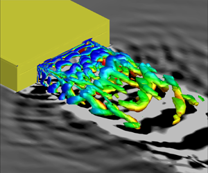
The response of the shear layer highlighting the vortical mechanisms in the controlled jets is first evaluated in figure 8. The phase-averaged Q-criterion coloured by streamwise velocity, $u$, are displayed at selected instances of the forcing time period. A time period of the forcing is used as the reference signal for phase averaging of the controlled jets. For comparison, the baseline jet is also included by phase averaging the flow field at $St=1$, starting from the first snapshot collected (since the baseline jet cannot be phase locked to any particular forcing signal). This first snapshot is collected after the simulation attains statistical stationarity. The columns in figure 8 correspond to baseline, M0, M1 and M2 forcings as indicated. The rows correspond to snapshots of the flow at four representative instances in the forcing cycle, $0 \le t_{f} \le T_{f}$, in terms of percentage of $t_{f}/T_{f}$. Here $T_{f}$ represents the time period of forcing and is defined as $1/St_{f}$, where $St_{f}$ is the non-dimensional frequency of forcing. In the controlled shear layers, the upward pointing solid red arrow tracks the vortical structure ‘A’ produced in the shear layer, while the downward pointing dashed red arrow tracks a different vortical structure, ‘B.’ When the actuators turn on at the start of a cycle, the extended vortical element A is created, which is parallel to the shear layer generated from the longer edge of the nozzle. Here B corresponds to structures that are produced when the actuators turn off, which eventually transform into lambda vortices.

Figure 8.

Phase-averaged flow features in the shear layer at indicated phases for the baseline and three forcing cases. The red solid and dashed arrows track vortices generated when an actuator is on and off, respectively.

Flow features occurring naturally at $St=1$ are limited to regions close to the nozzle exit in the baseline jet. In M0 actuation, lambda vortices, B, are stretched in the high-velocity core, while their ‘head’ region lags in the surrounding ambient fluid, as shown in figure 8(a). These ‘head’ regions later get pinched-off from the streamwise vortices, and interact with the trailing A vortical structure, forming a circumferentially connected element. These interactions result in a staggered pattern of vortices, as visible in the four instances of M0. The M1 actuation also exhibits a similar set of dynamics involving A and B vortical structures. The key difference here is that the lambda vortices and the circumferentially connected elements follow a helical pattern, due to the phase difference imposed on the consecutive actuators. However, the streamwise vortices in M1 is relatively weaker in comparison to M0. In M2 forcing, the streamwise strength of vortical elements are at par with that in M0. Furthermore, it also promotes higher helical modes in the consecutive sets of staggered lambda vortices. In essence, M2 forcing combines the advantages gained in M0 and M1 forcings, by generating stronger streamwise vorticity and higher helical modes. This enhances the 3-D nature of the shear layer response in a way conducive for noise source mitigation (Samimy et al. Reference Samimy, Webb, Esfahani and Leahy2023). Phase-averaged response of the shear layer in the M+/$-$1 forcing is similar to that achieved in the M0 forcing, and thus has been excluded for brevity. The primary difference is that the vortices produced in the upper and lower shear layers (on the longer edges) of the jet are in phase for M0 forcing, while they are out of phase in M+/$-$1 forcing.

Thus, the vortical effect of forcing on the shear layer is the production of streamwise-elongated lambda vortices, with the degree of three-dimensionality dependent on the mode of forcing. This reinforces the observation in § 4 that the shear layer is receptive to the spectrum in the vicinity of $St=1$, resulting in generation of vortices that scale with shear layer thickness. This provides the actuators the control authority necessary to tailor the evolution of coherent shear layer structures, and eventually, its acoustic signature. This is studied in the following section.

6.2. Acoustic response

Here we detail the acoustic response to forcing, in the plume and near field of the controlled jets. By near field we refer to the spatial region resolved in the ILES. Since hydrodynamic fluctuations attenuate rapidly in the radial direction from the jet centreline, the acoustic directivity in the near field can be evaluated using the dilatation field (Colonius, Lele & Moin Reference Colonius, Lele and Moin1997). However, in the plume, the energetic hydrodynamic fluctuations mask the acoustic response of the jet. Therefore, we extract the acoustic response in the plume of the controlled jets using Doak's momentum potential theory (Doak Reference Doak1989; Unnikrishnan & Gaitonde Reference Unnikrishnan and Gaitonde2016).

6.2.1. Acoustic response of the plume

The effect of actuation on the acoustically relevant fluctuations of the plume is isolated through a Helmholtz decomposition on the mass flux vector field ($\rho \boldsymbol {u}$). This segregates its solenoidal (hydrodynamic) and irrotational (acoustic and thermal) components, which can be represented using

(6.1)\begin{equation} \rho \boldsymbol{u} = \boldsymbol{\bar{B}} + \boldsymbol{B'} - \boldsymbol{\nabla} (\psi_{a}' + \psi_{T}'), \end{equation}

where $\bar {B}$ and $B'$ are the mean and fluctuating solenoidal components, respectively; $\psi _{a}'$ and $\psi _{T}'$ are the irrotational scalar potentials for the acoustic and thermal components, respectively. By utilizing the above relation in the continuity equation, the acoustic and thermal components of the flow can be extracted by solving the following Poisson equations:

(6.2a,b) \begin{equation} \nabla^2 \psi_a' = \frac{1}{c^2}\frac{\partial p}{\partial t}, \quad \nabla^2 \psi_T' = \frac{\partial \rho}{\partial S}\frac{\partial S}{\partial t}. \end{equation}

Here $c$ is the local speed of sound and $S$ is entropy. Additional details of the decomposition are available in Unnikrishnan & Gaitonde (Reference Unnikrishnan and Gaitonde2016). The streamwise component of acoustic fluctuations $(- {\partial \psi _{a}'}/{\partial x} )$ mostly determines the downstream radiated noise. Since the control is most effective in manipulating the downstream noise emissions (as will be shown later in § 8), the following discussions will focus on this streamwise component, which will be referred to as $A_{x}$, where $A_{x} = (- {\partial \psi _{a}'}/{\partial x} )$. As shown in Chakrabarti et al. (Reference Chakrabarti, Gaitonde and Unnikrishnan2021), this acoustically filtered component of the flow exhibits a wavepacket behaviour in rectangular jets.

The acoustic response (at the forcing frequency) in the plume is represented using phase-averaged iso-levels of $A_{x}$, as shown in figure 9. The projected views on the major and minor axis planes for the baseline jet are shown in figures 9(a) and 9(b), respectively. Corresponding results for M0 forcing (c,d), M1 forcing (e,f), M2 forcing (g,h) and M+/$-$1 forcing (i,j) are also included. The baseline jet has a limited acoustic signature at $St=1$, which is restricted to the near-nozzle regions. The M0 forcing results in an axially compact wavepacket, which reflects the AR of the nozzle. The acoustic response to M1 forcing is a helical wavepacket that sustains further downstream. The M2 forcing produces a ‘double helix’, with streamwise extent in between that of the M0 and M1 forcing. As will be evident in the following section, the double helix acoustic wavepacket contains two cycles of azimuthal oscillations at a given streamwise location. These acoustic responses in this low-AR rectangular jet draw a parallel with the responses observed in circular jets, when actuated using various azimuthal modes of LAFPA-based controllers (Gaitonde & Samimy Reference Gaitonde and Samimy2010; Gaitonde Reference Gaitonde2012). In response to M+/$-$1 forcing, the acoustic wavepacket has an anti-symmetric structure with respect to the major axis plane. This structure is similar to those observed in flapping rectangular jets, e.g. as discussed in Gojon et al. (Reference Gojon, Gutmark and Mihaescu2019). The streamwise extent of this wavepacket is longer than those excited by the other controlled jets. This evaluation demonstrates that the forcing pattern of the actuators has a strong influence on the 3-D form of the acoustic response of the plume.

Figure 9.

Instantaneous snapshot in the phase-averaged cycle of iso-levels of acoustic fluctuations at $A_{x} = \pm 0.005$ for the baseline jet, projected onto the (a) major axis plane and (b) minor axis plane. Plots (c,d) show the corresponding results for the M0 forcing; (e,f) are corresponding results for the M1 forcing; (g,h) are corresponding results for the M2 forcing; (i,j) are corresponding results for the M+/$-$1 forcing. The distance between consecutive vertical and horizontal grid lines are 2$D_{eq}$ and 1$D_{eq}$, respectively.

6.2.2. Acoustic directivity

The near-field acoustic response to forcing at $St=1$ is shown in figure 10, using phase-averaged contours of dilatation. Response to M0 forcing is represented at the middle of the actuator on phase, $t_{f}/T_{f}=0.25$, on the two principal planes of the jet. Two bands of acoustic radiation are produced on the minor axis plane. The dominant band propagates in the downstream direction, and eventually spreads across the propagation plane within $20^{\circ } \le \theta \le 60^{\circ }$, approximately centred around the red solid line. This band is induced by intrusion of vortical structures into the potential core (Unnikrishnan & Gaitonde Reference Unnikrishnan and Gaitonde2016), which are generated as a nonlinear shear layer response to the forcing (Lakshmi Narasimha Prasad & Unnikrishnan Reference Lakshmi Narasimha Prasad and Unnikrishnan2023b). The sideline direction (70$^{\circ } \le \theta \le 90^{\circ }$) is dominated by the second band of acoustic radiation, which is approximately centred around the blue dashed line in figure 10. This appears at the nozzle exit, and is a direct impact of the pressure fluctuations produced by the plasma actuator. While the spatial structure of the second (sideline) radiation band differs on the two principal planes, that of the first (downstream) is similar on both the planes, which is consistent with the above hypothesis. All the control cases studied here have this general form of near-field acoustic response on the principal planes at the forcing frequency. The main difference arises in the M+/$-$1 forcing, where the major axis plane has no significant response at the forcing frequency, due to the deactivated actuators on the shorter edges of the nozzle.

Figure 10.

Instantaneous snapshot in the phase-averaged cycle of dilatation contours at a phase of ${\rm \pi} /2$ on the (a) major and (b) minor axis planes for the M0 forcing. Eleven contour levels are evenly distributed between $-0.02$ and 0.02.

Azimuthal variations in the near-field acoustic response of the jets at the forcing frequency are best visualized on a streamwise plane, as shown in figure 11. Phase-averaged dilatation at $t_{f}/T_{f}=0.5$ is shown for M0, M1, M2 and M+/$-$1 controlled cases at $x \sim 4.5$, which encompasses the peak amplitudes in the downstream acoustic band (seen earlier in figure 10).

Figure 11.

Instantaneous snapshot in the phase-averaged cycle of dilatation contours at a phase of ${\rm \pi}$ for the (a) M0, (b) M1, (c) M2 and (d) M+/$-$1 forcings. Eleven contour levels are evenly distributed between $-0.01$ and 0.01.

The M0 forcing results in mostly concentric rings of acoustic radiation dominated by the axisymmetric mode, due to the synchronous firing of all actuators (figure 11a). Towards the near-field, the waves emitted from the longer edges display slightly higher amplitudes, which can be associated to the larger number actuators placed there. This acoustic response resembles the signature of two acoustic mono-poles separated by a small distance (Russell Reference Russell2013). The downstream acoustic imprint of M1 forcing is a spiral around the jet centreline, as seen in figure 11(b). This follows the phase lag in the vortex intrusion events generated from successive actuators, consistent with the spiral pattern seen earlier in the shear layer vortices in figure 8. Compared with M0 forcing, M1 forcing results in relatively lower amplitudes of acoustic response in the near-field. The M2 forcing generates a double helix radiation pattern, shown in figure 11(c), that further weakens the near-field imprint of forcing. The M+/$-$1 forcing results in acoustic waves that are anti-symmetric about the $z$ axis, as shown in figure 11(d). The out-of-phase action of the top and bottom set of actuators on the longer edges of the nozzle produces an acoustic dipole. Due to the destructive interference of these waves, the major axis plane experiences a reduction in the amplitude of forced acoustic response. These variations in the forced acoustic response of the jets have implications for far-field noise mitigation efforts, as will be later detailed in § 8.

7.1. Convective speed

As previously identified in the literature, turbulent jets sustain large-scale coherent structures, in addition to fine-scale turbulence (Crow & Champagne Reference Crow and Champagne1971; Brown & Roshko Reference Brown and Roshko1974; Michalke & Fuchs Reference Michalke and Fuchs1975; Arndt, Long & Glauser Reference Arndt, Long and Glauser1997). In high-speed jets, supersonic convection of such coherent structures, which are often viewed as instability waves, leads to Mach wave radiation (Tam Reference Tam1995; Nichols, Lele & Moin Reference Nichols, Lele and Moin2009), which significantly contributes to the acoustic signature of the jet. Therefore, here we evaluate the convective speed of acoustically relevant coherent structures using a wavenumber–frequency analysis.

Figure 12 shows the spatio-temporal Fourier transform of the acoustic component, $A_{x}$, in the near-field. The data are obtained from a horizontal array of probes placed $2.5D_{eq}$ away from the jet centreline, on the major axis plane. Data on the minor axis plane shows qualitatively similar trends, and are not included for brevity. The abscissa shows the streamwise wavenumber ($k$), the ordinate shows frequency ($St$) and the contour levels show the logarithm of energy. The streamwise wavenumber, $k$, is non-dimensionalized as $k=k^{*}D_{eq}^{*}$, where $k^{*}$ is the dimensional wavenumber and $D_{eq}^{*}$ is the nozzle equivalent diameter. Since the energy contribution from upstream propagating waves is substantially less than that from downstream propagating waves, only the positive wavenumbers are depicted in these contours. The convective speed is proportional to the slope, $St/k$, which is equivalent to ($1/2{\rm \pi}$)$\omega /k$, where $\omega$ is the non-dimensional circular frequency. Relevant phase speeds of the flow, $U_j-c_j$, $c_j$ and $U_j+c_j$, are shown using a blue dotted line, red dashed line and green dashed-dot line, respectively. Here, $U_j$ is the jet exit velocity and $c_j$ is the speed of sound based on jet exit conditions. Peak energy within this acoustic wavepacket propagates at a velocity of about $0.7U_{j}$, which is close to the jet exit sonic speed. Energy content that propagates at supersonic convective speeds and, thus, contributes to far-field acoustic emissions is located to the left of the red dashed line.

Figure 12.

Wavenumber–frequency spectra of acoustic fluctuations on the major axis plane for the (a) baseline jet, (b) M0 forcing, (c) M1 forcing, (d) M2 forcing and (e) M+/$-$1 forcing.

The acoustic wavepacket has most of the energy in the radiation zone (since the convective hydrodynamic component has been removed from this field). The baseline jet (figure 12a) displays energy peaks within $0.1 \le St \le 0.5$, with minimal radiation below $St \sim 0.1$. Although higher frequencies radiate, their energy content is significantly lesser than that in the vicinity of the jet column mode. In the controlled jets, the shear layer actuation, in general, reduces the above-mentioned column-mode peaks in the supersonic regime. With M0 forcing (figure 12b), energy reduction within the supersonic radiating band is achieved primarily at column-mode frequencies below $St \sim 0.4$, and at higher frequencies within $0.7 \le St \le 1$, in the vicinity of the forcing frequency. Similar inferences can be drawn for M1 forcing (figure 12c), where column-mode energy reduction is observed in the frequencies surrounding $St \sim 0.3$. The M2 forcing (figure 12d) shows the most attenuation in column-mode energy among all the controlled simulations studied. The peak energy bands seen in the baseline case have been significantly reduced with M2 control. Energy reduction achieved in M+/$-$1 forcing (figure 12e) is comparable to that in M0 forcing, at frequencies below $St \sim 0.4$.

Along with the reduction of supersonic energy content, actuation results in the fundamental tone, seen as a peak in the controlled cases. While M+/$-$1 forcing does not display this peak in the major axis plane, it is observed in the near-field acoustic component on the minor axis plane. Among these actuation patterns, M2 forcing exhibits minimal tonal amplitudes. This along with the most reduction in supersonic column-mode energy makes M2 forcing efficient at mitigating noise emissions.

Below we further quantify the energy reduction in the supersonic radiating regime of column-mode frequencies. The energy distribution across various convective speeds is plotted at two frequencies, $St=0.3$ and $St=0.4$, in figure 13. The abscissa displays the phase speed, and the ordinate is the logarithm of the power spectral density. Vertical lines identify significant phase speed values, corresponding to the slow acoustic wave (dotted line, $U_j-c_j$), sonic speed at the jet exit (solid line, $c_j$), jet exit velocity (dashed-dotted line, $U_j$) and the fast acoustic wave (dashed line, $U_j+c_j$). These plots are shown for both major (figure 13a,c) and minor axis planes (figure 13b,d). Energy content to the right of the solid black line has a supersonic convective wave speed and contributes to acoustic radiation, and is indicated by the red arrow.

Figure 13.

Distribution of the power spectral density with respect to phase speed at (a,b) $St=0.3$ and (c,d) $St=0.4$. Left and right columns correspond to major and minor axis planes, respectively.

Since the sampling location ($2.5D_{eq}$ away from the jet centreline) is closer to the shear layer on the major axis plane than that on the minor axis plane (due to the AR of the jet), fluctuation amplitudes and absolute energy content is slightly higher on the major axis plane. In the baseline jet, peak energy content is present within the supersonic phase speed. With control, this energy peak reduces to varying levels in all cases. For all the controlled jets, the energy reduction is higher on the major axis plane than on the minor axis plane. At $St=0.3$, the reduction levels are similar between the M1 and M+/$-$1 forcing on both planes. The M0 forcing shows the largest energy reduction at $St=0.3$ on the major axis plane, but M2 forcing is more consistent in achieving significant reductions in energy on both planes. At $St=0.4$, M0, M1 and M+/$-$1 forcings show similar levels of energy reduction on both planes, while M2 forcing has the largest reduction on both planes. Thus, the effect of control is to reduce the energy content within the supersonic radiating regime, with M2 forcing being the most effective forcing strategy.

7.2. Coherence of acoustic wavepackets

Advection of coherent turbulent structures in the jet mixing layer results in large-scale oscillations, which can be interpreted as wavepackets with specific growth and decay rates (Jordan & Colonius Reference Jordan and Colonius2013; Cavalieri, Jordan & Lesshafft Reference Cavalieri, Jordan and Lesshafft2019). They also behave as non-compact acoustic sources leading to noise characteristics with a distinct directivity (Sinha et al. Reference Sinha, Rodríguez, Brès and Colonius2014; Papamoschou Reference Papamoschou2018). The azimuthal coherence of these acoustic wavepackets have been shown to govern their radiating efficiency into the far field (Michalke & Fuchs Reference Michalke and Fuchs1975), with lower azimuthal modes being more efficient acoustic radiators. Thus, the impact of control on the spatio-temporal and azimuthal coherence of these wavepackets are studied via a 3-D spectral proper orthogonal decomposition (SPOD) (Towne, Schmidt & Colonius Reference Towne, Schmidt and Colonius2018; Schmidt & Colonius Reference Schmidt and Colonius2020) of the acoustic component. This is performed over a subdomain spanning $0 \le x \le 15$, $-2 \le y \le 2$ and $-2 \le z \le 2$. The parameters used for this decomposition are detailed in table 3.

Table 3.

Parameters used for spectral proper orthogonal decomposition.

The eigenvalue spectra for the leading two SPOD modes are shown in figures 14(a) and 14(b), respectively. For the baseline jet, a broadband peak exists between $0.15 \le St \le 0.4$, with peak eigenvalue magnitudes at $St \sim 0.3$, in both the leading modes. In the leading SPOD mode, control results in a broadband reduction of eigenvalue magnitudes within $0.15 \le St \le 0.45$ in all cases, and induces peaks at the forcing frequency, $St=1$, and its superharmonic, $St=2$. The M2 forcing achieves most reduction in eigenvalues near the column-mode frequencies, consistent with the energy reduction seen in wavenumber–frequency spectra. The M0 and M2 forcings also show reduction above column-mode frequencies, between $0.6 \le St \le 0.8$. Peaks at the forcing frequency and the superharmonic are minimal in the M2 forcing, consistent with previous observations. In the second SPOD mode, the effects of control are relatively smaller. However, a broadband reduction is seen with M0 and M2 forcings, while M1 and M+/$-$1 forcings show similar eigenvalue magnitudes as in the baseline jet. Furthermore, the forcing tones are completely accounted for in the leading SPOD mode, with minimal representation in the higher modes.

Figure 14.

(a,b) Eigenvalue spectra comparison for the first two most energetic modes, respectively. (c) Rank gap between the first two dominant modes.

The rank gap (defined as the difference between the leading two eigenvalues) provides a measure of the effectiveness of the control in redistributing energy across a broader range of spatio-temporal scales. Therefore, a smaller rank gap is a desirable quality to achieve noise source weakening. This is quantified in figure 14(c) for the baseline ad controlled jets. A significant gap exists between the two dominant SPOD modes of the acoustic component in the baseline jet, indicating a low-rank behaviour, particularly near the column mode. Control reduces this rank gap, with peak reduction in M2 forcing, observed in the spectral range, $0.15 \le St \le 0.4$, which contributes to the peak noise radiation from this jet. This redistribution of energy into subdominant modes of the acoustic wavepacket reduces the probability of coherent structures resulting in large-scale radiation events.

To evaluate the spatial coherence in the acoustic wavepacket, we now present the SPOD modes and its azimuthal composition. It has to be noted that although the near-nozzle shear layer is non-axisymmetric due to the nozzle geometry, the near-field acoustic component of this ${\rm AR}=2:1$ jet lends itself to efficient representation using azimuthal Fourier modes, centred around the jet centreline (Chakrabarti et al. Reference Chakrabarti, Gaitonde and Unnikrishnan2021). Key observations on its structure in the presence of control can be identified using a representative frequency, $St=0.3$. The acoustic wavepacket from the baseline case (figure 15a) is compared with that in M2 forcing (figure 15b) for brevity, since it shows the largest reduction in eigenvalue magnitudes near the column-mode frequencies. The azimuthal composition of each SPOD mode is identified using its Fourier decomposition, resulting in azimuthal modes. The first three azimuthal modes for each SPOD mode are included in the subsequent columns, to highlight key variations with control. The azimuthal decomposition is performed as

(7.1)\begin{equation} q(x, r, \phi)=q_{a}^{0}(x, r)+\sum_{m=1}^{\infty} [q_{a}^{m}(x, r) \cos (m \phi) + q_{b}^{m}(x, r) \sin (m \phi)], \end{equation}

where $m$ refers to the azimuthal mode number and $q_{a}^{m}(x, r)$ and $q_{b}^{m}(x, r)$ are the azimuthally invariant spatial supports determined by

(7.2)\begin{gather} q_{a}^{0}(x, r)=\frac{1}{2 {\rm \pi}} \int_{-{\rm \pi}}^{\rm \pi} q(x, r, \phi) \,{\rm d} \phi, \end{gather}

(7.3)\begin{gather} q_{a}^{m}(x, r)=\frac{1}{\rm \pi} \int_{-{\rm \pi}}^{\rm \pi} q(x, r, \phi) \cos (m \phi) \,{\rm d} \phi, \end{gather}

(7.4)\begin{gather} q_{b}^{m}(x, r)=\frac{1}{\rm \pi} \int_{-{\rm \pi}}^{\rm \pi} q(x, r, \phi) \sin (m \phi) \,{\rm d} \phi. \end{gather}

Azimuthal origin ($\phi = 0$) is set at the minor axis plane of the jet ($+$ve $y$ axis). For each azimuthal mode, suitable iso-levels are chosen to qualitatively describe its spatial extent. For quantitative comparisons, inset images with contours of $\sqrt {(q_{a}^{m})^{2}+(q_{b}^{m})^{2}}$ for each azimuthal mode are also shown. In the explanation that follows, the term ‘mode’ refers to the SPOD mode (column 1), whereas ‘$\phi$ mode’ refers to the azimuthal mode obtained through Fourier decomposition.

Figure 15.

(a) Iso-levels of the leading two SPOD modes of acoustic fluctuations in the baseline jet at a frequency of $St=0.3$, and its azimuthally decomposed Fourier modes. The first column shows the SPOD modes, while the subsequent columns show the corresponding three azimuthal Fourier modes. Plot (b) shows the same results for the M2 controlled jet. Inset figures below each azimuthal mode show contours of the corresponding spatial coefficients, $\sqrt {q_{a}^{2}+q_{b}^2}$. Spatial extent of the contour plots is $0 \le x \le 11$ and $0 \le r \le 2$. The ticks on the contour plot axes are spaced at $2D_{eq}$. Contour levels are uniformly distributed from $0.0001$ to $0.005$.

The coherent structures at $St=0.3$ in both the leading modes of the baseline have a dominantly axisymmetric nature. The spatially localized growth and decay of the acoustic wavepacket is consistent with findings on energetic structures by Arndt et al. (Reference Arndt, Long and Glauser1997) and Colonius & Freund (Reference Colonius and Freund2002) in circular jets, Chakrabarti et al. (Reference Chakrabarti, Gaitonde and Unnikrishnan2021); Lakshmi Narasimha Prasad & Unnikrishnan (Reference Lakshmi Narasimha Prasad and Unnikrishnan2023a) in rectangular jets and Lakshmi Narasimha Prasad et al. (Reference Lakshmi Narasimha Prasad, Saleh, Sellappan, Unnikrishnan and Alvi2022) in diamond jets. The axisymmetric $\phi$-mode 0 contains the majority of the energy due to the low AR of this jet. The spatial supports of $\phi$-mode 1 and $\phi$-mode 2 show a depreciating trend. The higher $\phi$ modes are mostly confined to the corners of the nozzle.

The M2 forcing enhances the higher $\phi$ modes of the acoustic wavepacket, as seen in figure 15(b). While mode 1 still retains a largely axisymmetric behaviour, its $\phi$-mode 1 shows significant amplification in relation to the baseline. This azimuthal redistribution of energy is more evident in mode 2, where the spatial support of $\phi$-mode 0 is severely attenuated, and confined towards the core of the jet near the centreline. Its $\phi$-mode 1 has a stronger spatial support as evidenced by the higher intensities in the spatial coefficients, visible in the corresponding inset contour. Its $\phi$-mode 2 also undergoes amplification, particularly away from the nozzle exit. Therefore, M2 forcing facilitates percolation of energy from $\phi$-mode 0 into $\phi$-mode 1 and 2. This modification to the dominant acoustic modes of the jet is beneficial (Michalke & Fuchs Reference Michalke and Fuchs1975), since lower/higher azimuthal modes have higher/lower downstream radiative efficiency. Thus, control not only redistributes energy into subdominant modes, it also redistributes energy into higher $\phi$ modes, which is favourable for reducing noise radiation from the jet.

7.3. Nonlinear interactions

As seen in the preceding spectral analysis, the actuation results in redistribution of acoustic energy into the forcing frequencies and its harmonics. These phenomena occur through nonlinear interactions that manipulate spectral and azimuthal content in the acoustic wavepackets, which is the focus of this section.

To identify the azimuthal and spectral distribution of energy in the controlled jets, the acoustic component, $A_{x}$, is first subjected to an azimuthal decomposition, which extracts its $\phi$ modes. Following this, SPOD is performed on each of the first ten $\phi$ modes. The resulting eigenvalue spectra of the leading SPOD mode for the first six $\phi$ modes are shown in figure 16. Results are presented for the M0 and M1 forcing, due to their unique response patterns. The abscissa shows frequency ($St$) while the ordinate represents the $\phi$ modes. The contour levels depict the logarithm of the eigenvalue magnitude obtained from the decomposition. In the following, the frequency-azimuthal response is represented using the ordered pair, $(n_{St},n_{m})$. Here, $n_{St}$ is the ‘$n$th’ harmonic of the forcing (e.g. $n_{St}=1$ represents the forcing frequency); $n_{m}$ represents the ‘$n$th’ azimuthal mode (e.g. $n_{m}=0$ corresponds to the axisymmetric $\phi$ mode).

Figure 16.

Eigenvalue spectra at various $\phi$ modes for (a) M0 control and (b) M1 control.

The M0 forcing (figure 16a) excites $(1,0)$ as expected, indicating that the wavepacket has a largely axisymmetric structure, consistent with the forcing wavepacket seen in § 6.2.1. Higher even $\phi$ modes ($(1,2)$, $(1,4)$, etc.) are also excited due to the combined effects of the nozzle AR and corner vortices, but with progressively lower magnitudes. The superharmonic, $(2,0)$, and its higher even $\phi$ modes are also exited with M0 forcing. The M2 forcing also results in a similar pattern, and is not included for brevity. The M1 forcing (figure 16b) generates odd $\phi$ modes $(1,1)$, $(1,3)$, $(1,5)$, etc., at the fundamental forcing frequency. However, its superharmonic frequency exists at even $\phi$ modes, $(2,0)$, $(2,2)$, $(2,4)$, etc.

Since the spectrum of the forcing signal does not contain energy at $St=2$, as seen earlier in figure 3, the above superharmonic is a result of nonlinear interactions in the flow response. In the following, we characterize these nonlinear interactions in the jet plume, by evaluating dominant triadic interactions within the acoustic wavepacket, using bi-spectral analysis. The bi-spectrum identifies genesis of a new frequency/wavenumber resulting from nonlinear interactions of two other frequencies/wavenumbers (Kim et al. Reference Kim, Beall, Powers and Miksad1980; Nekkanti et al. Reference Nekkanti, Schmidt, Maia, Jordan, Heidt and Colonius2023). The results are obtained using a bi-spectral mode decomposition as detailed in Schmidt (Reference Schmidt2020), on the 3-D field of the acoustic component, $A_{x}$.

The bi-spectrum for the baseline and M0, M1, M2 forcing cases are presented in figures 17(a), 17(b), 17(c) and 17(d), respectively. The abscissa and ordinate show a set of frequencies that nonlinearly interact and generate a third frequency, which is interpreted as the sum of the interacting frequency pair. The red dashed slanted lines demarcate all the pair of interactions that nonlinearly generate frequencies surrounding the jet column mode, between $0.15 \le St \le 0.4$, which are responsible for peak noise levels. The negative axis of frequencies represent difference interactions between the relevant pair.

Figure 17.

(Magnitude) mode bi-spectrum for the (a) baseline jet, (b) M0 forcing, (c) M1 forcing and (d) M2 forcing. The red dashed line corresponds to frequencies around the jet column mode.

The baseline case (figure 17a) has high magnitudes in the above-mentioned column-mode band, that nonlinearly energizes the dominant acoustic response of the jet. An interesting observation is that the column-mode band is mostly generated due to the difference interactions of relatively higher frequencies. In comparison to the baseline case, nonlinear generation of the column-mode band is progressively reduced in the M0, M1 and M2 forcings, with the M2 forcing achieving the most reduction of almost one order of magnitude. The bi-spectrum of the controlled cases also confirms that the energy peak at $St=2$ is generated from the sum interaction of the forcing frequency (i.e. $f1=1$, $f2=1$, $f3=f1+f2=2$).

The following wave interaction is used to demonstrate that the superharmonic, $St=2$, will mostly sustain even $\phi$ modes irrespective of the azimuthal nature of forcing. Consider a wave with unit amplitude of the form

(7.5)\begin{equation} g(m,\omega)=\exp({{\rm i}(m\phi - \omega t)}), \end{equation}

where $m$ is the positive or negative integer azimuthal mode number and $\omega$ is the circular frequency. Using the relation, $\omega = 2 {\rm \pi}f$,

(7.6)\begin{equation} g(m,f)=\exp({{\rm i}(m\phi - 2 {\rm \pi}f t)}), \end{equation}

where $f$ is the non-dimensional frequency ($St$). Nonlinear interaction of two such waves at frequencies, $f_{1}$ and $f_{2}$, and azimuthal modes, $m_{1}$ and $m_{2}$, can be represented as

(7.7)\begin{align} g(m_{1},f_{1})g(m_{2},f_{2})&=\exp({{\rm i}(m_{1}\phi - 2 {\rm \pi}f_{1} t)})\exp({{\rm i}(m_{2}\phi - 2 {\rm \pi}f_{2} t)})\nonumber\\ &=\exp({{\rm i}(m_{1} + m_{2})\phi})\exp({-{\rm i}2{\rm \pi}(f_{1} + f_{2})t}). \end{align}

Considering a resultant frequency, $f_{1} + f_{2}=2$, as in the bi-spectrum above,

(7.8)\begin{equation} g(m_{3},2)=\exp({{\rm i}(m_{3}\phi - 4 {\rm \pi}t)}), \end{equation}

where $m_{3} = m_{1} + m_{2}$. For M0 forcing, the $\phi$ modes dominant at the forcing frequency are $m=0,\pm 2, \pm 4,$ etc. Therefore, their mutual interactions, $m_{3} = m_{1} + m_{2}$, are either zero or are even integers, as observed in figure 16(a). The M1 forcing results in $\phi$ modes, $m=\pm 1,\pm 3, \pm 4,$ etc. Again, any combination of these modes always yields either a zero or an even integer, causing the superharmonic frequency to possess an even $\phi$ mode structure.

These observations highlight the fact that there are significant spatio-temporal nonlinearities that energize the column-mode frequencies. Localized arc filament plasma actuator based control can subdue those triadic interactions responsible for peak noise radiation, and can nonlinearly modify the azimuthal structure of the acoustic wavepacket.

7.4. Intermittency

Intermittent events resulting in bursts of acoustic energy contribute significantly to the peak far-field noise levels of the jet (Crawley & Samimy Reference Crawley and Samimy2014). To identify the effect of control on acoustically relevant intermittency, we utilize a Morse wavelet (Lilly & Olhede Reference Lilly and Olhede2009, Reference Lilly and Olhede2012) transform on the near-field acoustic component. Data are sampled on the major and minor axis planes at $\theta \sim 32^{\circ }$, $2.5D_{eq}$ away from the jet centreline. Results are shown in figure 18, using contours of the wavelet coefficient magnitude. The red solid line demarcates the cone of influence that separates the accurate region (within the cone) from the erroneous zone (outside the cone), resulting from wavelets that extend past the boundaries of the observation interval. Since frequencies $0.15 \le St \le 0.4$ are the most energetic and contribute to peak noise levels, events occurring in this band are of interest and are shown by the red dashed lines in the contours.

Figure 18.

Scalograms of the acoustic fluctuations at $r=2.5$, $\theta \sim 32^{\circ }$, on the major axis and minor axis planes. Solid red curves demarcate the cone of influence, while the horizontal dashed red lines highlight the frequency band of interest.

The acoustic component in the baseline jet contains several energetic intermittent events on both the major and minor axis planes (within the frequency band of interest), which directly contribute to far-field sound (Unnikrishnan & Gaitonde Reference Unnikrishnan and Gaitonde2016). Control reduces these intermittent events, with the degree of reduction depended on the forcing strategy. The M0 and M1 forcing shows intermittency reduction on both planes, with M0 being relatively more effective. The M2 forcing is the most successful in reducing intermittent acoustic events, with the best performance achieved on the minor axis plane, in terms of minimizing the amplitude and number of occurrences of intermittent events. In M+/$-$1 forcing, intermittency reduction is evident on the minor axis plane, but not on the major axis plane, due to the forcing pattern. Furthermore, all the controlled jets display increased intermittency at the forcing frequency, resulting from the downstream acoustic band, shown earlier in figure 10.

In order to better quantify intermittency effects, histograms are plotted in figure 19. The ordinate corresponds to the ratio of the number of occurrences in a specific bin to the overall number of occurrences, and the abscissa denotes the scalogram magnitude. Thus, the plots represent the probability of occurrence of these time-frequency localized events between the frequency bands of interest ($0.15 \le St \le 0.4$) shown in figure 18. The brown solid line demarcates a threshold chosen to identify an energetic intermittent event in this frequency band. This representative threshold of $7 \times 10^{-4}$ is close to the upper limit of the contour levels shown in figure 18. Thus, bins to the right of this threshold identify strong intermittent events that are of interest.

Figure 19.

Histograms depicting probability of occurrence of time-frequency localized events between $0.15 \le St \le 0.4$ at various scalogram magnitudes on the (a) major axis plane and (b) minor axis plane. The solid brown line represents the threshold of the scalogram magnitude chosen to quantify a significant event. The red arrow denotes the region of interest.

The baseline histogram in figure 19 shows high probability of energetic intermittent events, which are reduced upon forcing the jet. For example, compared with the baseline case, M2 forcing has a cumulative reduction of ${\sim }65\,\%$ and ${\sim }55\,\%$ on the major and minor axis planes, respectively. Other controlled cases also follow similar trends, as identified in the preceding discussion on scalograms. Along with the reduction in high-amplitude events, the histograms also show a shift in peak probability to lower wavelet coefficient magnitudes. This indicates that, even if these intermittent events were to occur within the jet, the energy content, and hence, their far-field noise signature will be much lower. This shift is quantified through the skewness values of the histograms, that highlight the asymmetry in the distribution. The baseline jet has a skewness of $0.269$ and $-0.196$ on the major and minor axis planes, respectively. A negative skewness indicates that the mode of the distribution is located to the right of its mean (i.e. higher wavelet coefficient magnitude), and has a long tail towards the left of the distribution (i.e. lower wavelet coefficient magnitude). With the imposition of M2 control for example, the skewness increases to $0.717$ on the major axis plane and $0.590$ on the minor axis plane. This indicates that the mode has shifted to the left of the mean (i.e. lower wavelet coefficient magnitude) with a long narrow tail to the right. The steeper probability roll off in controlled cases at high scalogram magnitudes demonstrates that the likelihood of intermittent events that produce sound waves at peak energy-containing frequencies has decreased.

Thus, the foregoing analyses has identified that, by (a) reducing energy in the supersonic regime at peak radiating frequencies and redistributing it into an energy band at the forcing frequency, (b) exciting higher azimuthal modes and smaller spatial scales, (c) reducing the energization of column-mode frequencies by limiting nonlinear triadic interactions, and (d) reducing extreme intermittent events within the jet that are responsible for bursts of acoustic energy, the control (in particular, M2 forcing) is successful in achieving a flow response conducive to noise mitigation.