





1. Introduction
Flow past a circular cylinder is both a rich physical phenomenon and a canonical benchmark for turbulence modelling. Across Reynolds number $ \textit{Re} \approx 300$
–
$ \textit{Re} \approx 300$
– $300{\,}000$
, the wake is fully turbulent while the boundary layer remains laminar. Classical Reynolds-averaged Navier–Stokes (RANS) closures – constrained by the assumptions used to close the Reynolds-stress term – struggle to predict the mean field and, more critically, the Reynolds stresses. By contrast, direct numerical simulation (DNS) resolves all dynamically relevant scales at low to moderate
$300{\,}000$
, the wake is fully turbulent while the boundary layer remains laminar. Classical Reynolds-averaged Navier–Stokes (RANS) closures – constrained by the assumptions used to close the Reynolds-stress term – struggle to predict the mean field and, more critically, the Reynolds stresses. By contrast, direct numerical simulation (DNS) resolves all dynamically relevant scales at low to moderate $ \textit{Re}$
, while at higher
$ \textit{Re}$
, while at higher $ \textit{Re}$
particle image velocimetry (PIV) provides spatially resolved measurements of mean velocity and Reynolds stresses, albeit over limited windows. These observations motivate two questions: (i) How can we infer full-field, physically consistent flow states from sparse, patchwise PIV data; and (ii) how can we overcome the structural limitations of classical RANS closures so that both the mean flow as well as the turbulent contribution are predicted accurately?
$ \textit{Re}$
particle image velocimetry (PIV) provides spatially resolved measurements of mean velocity and Reynolds stresses, albeit over limited windows. These observations motivate two questions: (i) How can we infer full-field, physically consistent flow states from sparse, patchwise PIV data; and (ii) how can we overcome the structural limitations of classical RANS closures so that both the mean flow as well as the turbulent contribution are predicted accurately?
Drawbacks of RANS closure: the Boussinesq assumption collapses the full Reynolds-stress tensor to an isotropic eddy-viscosity response, $\tau _{\textit{ij}} = 2\nu _t S_{\textit{ij}} - ({2}/{3})k\,\delta _{\textit{ij}}$
, where
$\tau _{\textit{ij}} = 2\nu _t S_{\textit{ij}} - ({2}/{3})k\,\delta _{\textit{ij}}$
, where $\tau_{\textit{ij}}$
for Reynolds stress tensor,
$\tau_{\textit{ij}}$
for Reynolds stress tensor, $\nu_t$
for turbulence viscosity,
$\nu_t$
for turbulence viscosity, $S_{\textit{ij}}$
for strain rate tensor,
$S_{\textit{ij}}$
for strain rate tensor, $k$
for turbulence kinetic energy and
$k$
for turbulence kinetic energy and $\delta_{\textit{ij}}$
for Kronecker delta. In flows with strong streamline curvature, rotation or rapid distortion, the true stress anisotropy departs markedly from this linear form, as shown by Schmitt (Reference Schmitt2007), leading to discrepancies in separation location, pressure distribution and global forces. These errors persist even when
$\delta_{\textit{ij}}$
for Kronecker delta. In flows with strong streamline curvature, rotation or rapid distortion, the true stress anisotropy departs markedly from this linear form, as shown by Schmitt (Reference Schmitt2007), leading to discrepancies in separation location, pressure distribution and global forces. These errors persist even when $\nu _t$
is calibrated to match a single target, because the structural restriction is the dominant error source. Nonlinear turbulence models, such as those introduced by Cambon & Scott (Reference Cambon and Scott1999) and Spalart (Reference Spalart2000), extend the Boussinesq hypothesis by allowing the Reynolds-stress anisotropy to depend on nonlinear combinations of the mean strain and rotation rate tensors, so they can represent effects like curvature, rotation and secondary flows that linear eddy-viscosity models miss. Coefficients may come from asymptotic analysis and calibration or from data-driven fitting. Limitations include sensitivity to coefficient choices and potential stiffness or instability if not embedded in conservative solver formulations with appropriate limiters. Nonlinear turbulence closures are still far from accurately matching both mean flow and Reynolds stress. Instead of representing the full Reynolds-stress tensor, one can model the Reynolds forcing vector, as shown by Amarloo et al. (Reference Amarloo, Forooghi and Abkar2022, Reference Amarloo, Cinnella, Iosifidis, Forooghi and Abkar2023), the net turbulent contribution that appears as a source term in the mean momentum equations. This targets what the solver directly requires, and integrates cleanly into RANS/unsteady RANS (URANS) by adding a learned body force at each control volume. It avoids tensor realisability constraints and is straightforward to supervise from DNS/large eddy simulation (LES) and PIV. This approach also supports a residual-learning variant, where the forcing vector is decomposed into a baseline Boussinesq part plus a learned correction, achieving both numerical stability and accuracy in the Reynolds forcing.
$\nu _t$
is calibrated to match a single target, because the structural restriction is the dominant error source. Nonlinear turbulence models, such as those introduced by Cambon & Scott (Reference Cambon and Scott1999) and Spalart (Reference Spalart2000), extend the Boussinesq hypothesis by allowing the Reynolds-stress anisotropy to depend on nonlinear combinations of the mean strain and rotation rate tensors, so they can represent effects like curvature, rotation and secondary flows that linear eddy-viscosity models miss. Coefficients may come from asymptotic analysis and calibration or from data-driven fitting. Limitations include sensitivity to coefficient choices and potential stiffness or instability if not embedded in conservative solver formulations with appropriate limiters. Nonlinear turbulence closures are still far from accurately matching both mean flow and Reynolds stress. Instead of representing the full Reynolds-stress tensor, one can model the Reynolds forcing vector, as shown by Amarloo et al. (Reference Amarloo, Forooghi and Abkar2022, Reference Amarloo, Cinnella, Iosifidis, Forooghi and Abkar2023), the net turbulent contribution that appears as a source term in the mean momentum equations. This targets what the solver directly requires, and integrates cleanly into RANS/unsteady RANS (URANS) by adding a learned body force at each control volume. It avoids tensor realisability constraints and is straightforward to supervise from DNS/large eddy simulation (LES) and PIV. This approach also supports a residual-learning variant, where the forcing vector is decomposed into a baseline Boussinesq part plus a learned correction, achieving both numerical stability and accuracy in the Reynolds forcing.
Data-driven turbulence closure: recent data-driven closures promise richer stress representations, including augmentation of the classical RANS models, such as Singh & Duraisamy (Reference Singh and Duraisamy2016) and Yan et al. (Reference Yan, Li, Zhang and Chen2022), direct prediction of the eddy viscosity, such as Zhu et al. (Reference Zhu, Zhang, Kou and Liu2019), prediction of the anisotropic part of Reynolds stresses, see Ling, Kurzawski & Templeton (Reference Ling, Kurzawski and Templeton2016) and Zhang et al. (Reference Zhang, Xiao, Luo and He2022), discrepancy of Reynolds stresses, see Wang, Wu & Xiao (Reference Wang, Wu and Xiao2017) and Li et al. (Reference Li, Tang, Yi and Yan2022), and the Reynolds forcing vector, see Cruz et al. (Reference Cruz, Thompson, Sampaio and Bacchi2019) and Amarloo et al. (Reference Amarloo, Cinnella, Iosifidis, Forooghi and Abkar2023). There are many issues of the data-driven turbulence closure models. It is now well recognised that purely a priori data fitting of Reynolds stresses or modelled forces, in which machine-learning models are trained to match high-fidelity data in an offline manner, often fail to deliver accurate predictions of quantities of interest (QoIs) once embedded in a computational fluid dynamics (CFD) solver. Despite achieving low regression error against DNS or LES targets, such models may lead to large discrepancies in integrated or flow-level metrics, including mean velocities, separation characteristics and force coefficients. This inconsistency arises because the learned closures are optimised independently of the governing equations and the numerical discretisation in which they are ultimately deployed. In contrast, a posteriori training strategies explicitly couple the learning process with the flow solver and typically optimise the model parameters with respect to QoIs directly, rather than enforcing pointwise agreement with Reynolds stresses or forcing terms. As a result, a posteriori approaches generally do not aim to reproduce the true underlying stress or force fields, but instead seek closures that compensate for both modelling deficiencies and structural errors inherent in the chosen model form, leading to improved predictive performance at the level of QoIs. Moreover, while the circular cylinder is one of the most extensively studied benchmark problems in fluid mechanics, data-driven turbulence closure studies on cylinder flows remain comparatively scarce, highlighting an important gap between canonical CFD validation cases and current machine-learning-based modelling efforts. Therefore, our focus is to pursue a closure discovery that is accurate both in mean flow and turbulence statistics for cylinder flows. Eddy-viscosity-based methods, including direct prediction and augmentation of RANS models, are not enough to fully represent the Reynolds stresses or force vector. Among the Reynolds stresses and the forcing vector, we choose to approximate the forcing vector directly because the turbulent contribution to the governing equation will be directly modelled without the divergence operator, and there are fewer degrees of freedom than in the Reynolds stresses.
Physics-informed neural networks (PINNs) and flow inference: PINNs provide a flexible way to fuse sparse and noisy measurements with the governing equations to recover hidden or unmeasured features of a flow, as shown by Toscano et al. (Reference Toscano, Käufer, Wang, Maxey, Cierpka and Karniadakis2025), Shukla et al. (Reference Shukla, Di Leoni, Blackshire, Sparkman and Karniadakis2020), Shukla et al. (Reference Shukla, Zou, Chan, Pandey, Wang and Karniadakis2025), Kiyani et al. (Reference Kiyani, Shukla, Karniadakis and Karttunen2023), Kiyani et al. (Reference Kiyani, Kooshkbaghi, Shukla, Koneru, Li, Bravo, Ghoshal, Karniadakis and Karttunen2024) and Karniadakis et al. (Reference Karniadakis, Kevrekidis, Lu, Perdikaris, Wang and Yang2021). In PINNs, a neural network represents one or more fields (e.g. velocity, pressure and possibly auxiliary closure terms), and minimises a composite loss that balances data mismatch at sensor locations, residuals of the partial differential equation (PDE) operator (e.g. momentum and continuity) and boundary/initial-condition penalties. Because the governing physics enters as soft constraints, PINNs naturally enable: flow inference (estimating latent quantities such as pressure or Reynolds stresses from velocity-only PIV data); flow reconstruction (extending partially observed subdomains to solver-ready, domain-wide fields); and flow super-resolution (lifting coarse spatial or temporal measurements to finer resolutions while respecting physical conservation laws). For example, Cai et al. (Reference Cai, Wang, Fuest, Jeon, Gray and Karniadakis2021) reconstructed three-dimensional velocity and pressure fields from tomographic background-oriented schlieren measurements and validated the inferred fields against independent PIV experiments; Patel et al. (Reference Patel, Mons, Marquet and Rigas2024) recovered the mean-flow velocity for flow past a cylinder at $ \textit{Re}=200$
; Eivazi et al. (Reference Eivazi, Tahani, Schlatter and Vinuesa2022) solved the RANS equations using sparse in-domain flow measurements; Hanrahan, Kozul & Sandberg (Reference Hanrahan, Kozul and Sandberg2023) demonstrated that embedding the RANS equations within PINNs enables accurate reconstruction of turbulent mean flows from measurement densities representative of experimental campaigns; and Eivazi, Wang & Vinuesa (Reference Eivazi, Wang and Vinuesa2024) showed that physics-informed deep-learning models can reconstruct and super-resolve flow fields from experimental data, including time-resolved hot-wire anemometry and PIV measurements.
$ \textit{Re}=200$
; Eivazi et al. (Reference Eivazi, Tahani, Schlatter and Vinuesa2022) solved the RANS equations using sparse in-domain flow measurements; Hanrahan, Kozul & Sandberg (Reference Hanrahan, Kozul and Sandberg2023) demonstrated that embedding the RANS equations within PINNs enables accurate reconstruction of turbulent mean flows from measurement densities representative of experimental campaigns; and Eivazi, Wang & Vinuesa (Reference Eivazi, Wang and Vinuesa2024) showed that physics-informed deep-learning models can reconstruct and super-resolve flow fields from experimental data, including time-resolved hot-wire anemometry and PIV measurements.
Contributions: this paper is organised as follows. After the introduction and problem set-up in § 2, we build a diverse dataset for flows past a cylinder using PIV and DNS/LES and introduce a physics-informed data correction method in § 3. We use PINNs with the unclosed RANS equation to infer the full-field flow states and Reynolds forcing based on only the boundary information in § 4. We then build a data-driven turbulence closure model based on the universality of Reynolds-stress distribution, and integrate it with a forward PINN solver and the numerical solver OpenFOAM in § 5. Finally, we draw the conclusion in § 6.
In summary, our contributions are:
-
(i) Diverse dataset. We assemble a multi-regime cylinder dataset combining incompressible and compressible DNS/LES and PIV, covering a broad Reynolds number range.
-
(ii) Flow inference with sparse data. We use PINNs to infer the full-field mean velocity and Reynolds forcing from boundary information, solving a numerically under-determined problem.
-
(iii) Universality of Reynolds stresses. We find that the distribution of Reynolds stresses/forcing is similar among the Reynolds numbers for both incompressible and weakly compressible flows past a cylinder.
-
(iv) Turbulence model discovery. We propose and evaluate data-driven closures that target simultaneous accuracy in Reynolds forcing and mean velocity.
-
(v) Turbulence model–solver integration. We integrate the data-driven closure model with both PINNs and OpenFOAM and find that the proposed data-driven closure model can improve the accuracy in both mean velocity and the Reynolds stresses.
2. Problem set-up
The flow past a cylinder is the focus of this study. The flow equations are normalised by the cylinder diameter $D$
and free-stream velocity
$D$
and free-stream velocity $U_\infty$
. In all set-ups, the origin of the two-dimensional coordinate system is at the centre of the cylinder. Hydrodynamic and aerodynamic PIVs are used to measure the mean-flow fields and turbulence statistics in the wake region. High-fidelity spectral-element-based DNS and LES are also conducted in a wide range of Reynolds numbers for both incompressible and weakly compressible regimes.
$U_\infty$
. In all set-ups, the origin of the two-dimensional coordinate system is at the centre of the cylinder. Hydrodynamic and aerodynamic PIVs are used to measure the mean-flow fields and turbulence statistics in the wake region. High-fidelity spectral-element-based DNS and LES are also conducted in a wide range of Reynolds numbers for both incompressible and weakly compressible regimes.
Figure 1 shows a sketch of the overview of our work. There are three primary aims in this paper: (i) build a diverse dataset for flows past a cylinder using PIV and DNS/LES. (ii) Infer the flow field and the Reynolds forcing using limited measurements and PINNs. (iii) Build data-driven turbulence closure models and integrate them with PINNs and numerical solvers.
Overview of the paper. (a) The PIV and DNS/LES are used to establish a dataset of flow past a cylinder. The range of the key parameters, $ \textit{Re}$
and Mach number
$ \textit{Re}$
and Mach number $Ma$
, is listed. (b) The PINNs are used to infer the flow fields within a domain
$Ma$
, is listed. (b) The PINNs are used to infer the flow fields within a domain $\varOmega$
based on the unclosed RANS equation and the boundary conditions (BC) at
$\varOmega$
based on the unclosed RANS equation and the boundary conditions (BC) at $\partial \varOmega$
for both incompressible and weakly compressible regimes. (c) Data-driven turbulence closure model is built and integrated with the forward PINN solver and the numerical solver OpenFOAM, investigating the accuracy of both velocity and Reynolds forcing fields.
$\partial \varOmega$
for both incompressible and weakly compressible regimes. (c) Data-driven turbulence closure model is built and integrated with the forward PINN solver and the numerical solver OpenFOAM, investigating the accuracy of both velocity and Reynolds forcing fields.

One of the key ideas in this paper is to use the unclosed data-driven RANS equation without any assumptions on the turbulence closure and to represent the Reynolds forcing directly. In this case, we can simultaneously pursue the accuracy of both velocity and Reynolds forcing fields. The steady two-dimensional unclosed RANS equation with Reynolds forcing for incompressible flows is
 \begin{align} \begin{aligned} \frac {\partial U}{\partial x}+\frac {\partial V}{\partial y}=0,\\ U \frac {\partial U}{\partial x}+V \frac {\partial U}{\partial y}+\frac {1}{\rho } \frac {\partial P}{\partial x}-\nu \left (\frac {\partial ^2 U}{\partial x^2}+\frac {\partial ^2 U}{\partial y^2}\right )-F_x=0, \\ U \frac {\partial V}{\partial x}+V \frac {\partial V}{\partial y}+\frac {1}{\rho } \frac {\partial P}{\partial y}-\nu \left (\frac {\partial ^2 V}{\partial x^2}+\frac {\partial ^2 V}{\partial y^2}\right )-F_y=0, \end{aligned} \end{align}
where $U,V,P$
are time-averaged state variables,
$U,V,P$
are time-averaged state variables, $\nu$
is the molecular viscosity and
$\nu$
is the molecular viscosity and $\rho =1$
is the density. Here,
$\rho =1$
is the density. Here, $F_x,F_y$
are the Reynolds forcing vectors, defined by
$F_x,F_y$
are the Reynolds forcing vectors, defined by $\boldsymbol{F} = \boldsymbol{\nabla }\boldsymbol{\cdot }\tau _{Re}$
, where
$\boldsymbol{F} = \boldsymbol{\nabla }\boldsymbol{\cdot }\tau _{Re}$
, where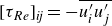 $[\tau _{Re}]_{\textit{ij}}=-\overline {u'_iu'_{\kern-1pt j}}$
is the Reynolds-stress tensor.
$[\tau _{Re}]_{\textit{ij}}=-\overline {u'_iu'_{\kern-1pt j}}$
is the Reynolds-stress tensor.
3. Data generation and cross-validation
3.1. Hydrodynamic particle image velocimetry
The hydrodynamic PIV experiments were performed using the robotic towing tank facility at the Massachusetts Institute of Technology. A detailed description of the facility can be found in Fan et al. (Reference Fan, Jodin, Consi, Bonfiglio, Ma, Keyes, Karniadakis and Triantafyllou2019). The towing tank has a length of 10 m in the main towing direction and a cross-section of 1 m $\times$
1 m.
$\times$
1 m.
A vertically mounted cylinder with a diameter $D=50.8$
mm is towed by a gantry robot that is mounted on a rail system at the top of the towing tank. The cylinder is made from aluminium and has a smooth surface, which is anodised in black to reduce light reflection on the cylinder’s surface. Endplates are attached to mitigate the effects arising from the finite extent of the cylinder and the free surface, resulting in an effective length between the endplates of
$D=50.8$
mm is towed by a gantry robot that is mounted on a rail system at the top of the towing tank. The cylinder is made from aluminium and has a smooth surface, which is anodised in black to reduce light reflection on the cylinder’s surface. Endplates are attached to mitigate the effects arising from the finite extent of the cylinder and the free surface, resulting in an effective length between the endplates of $L\approx 0.6$
m, which corresponds to an aspect ratio
$L\approx 0.6$
m, which corresponds to an aspect ratio $L/D=12$
. The camera (Optronis Cyclone 2000) and the lens (Zeiss Dimension 2/35) are mounted behind the cylinder in a waterproof housing. The camera images a horizontal light sheet perpendicular to the cylinder’s main axis, which is generated by a 40 W pulsed continuous wave laser (Optolutions LD-PS/40), fixed onto the gantry robot but positioned outside the towing tank. Thus, the relative position between the camera, cylinder and laser is fixed. To visualise the flow, polyamide particles of size 5
$L/D=12$
. The camera (Optronis Cyclone 2000) and the lens (Zeiss Dimension 2/35) are mounted behind the cylinder in a waterproof housing. The camera images a horizontal light sheet perpendicular to the cylinder’s main axis, which is generated by a 40 W pulsed continuous wave laser (Optolutions LD-PS/40), fixed onto the gantry robot but positioned outside the towing tank. Thus, the relative position between the camera, cylinder and laser is fixed. To visualise the flow, polyamide particles of size 5 ${\unicode{x03BC}}$
m were used, which over the duration of the experiment showed negligible floating or sedimentation. A camera calibration was performed to obtain the pixel scaling factor and compensate for optical distortions. The camera calibration resulted in a pixel scaling factor of 5.744 pixels/mm. The images were recorded as time series, and the time step
${\unicode{x03BC}}$
m were used, which over the duration of the experiment showed negligible floating or sedimentation. A camera calibration was performed to obtain the pixel scaling factor and compensate for optical distortions. The camera calibration resulted in a pixel scaling factor of 5.744 pixels/mm. The images were recorded as time series, and the time step $\Delta t$
between the frames was adapted to the Reynolds number and is shown in table 1. Due to the struts of the towing tank, the laser light is occasionally blocked. These events were discarded during the preprocessing. To provide a variety of data, runs at several different Reynolds numbers were performed.
$\Delta t$
between the frames was adapted to the Reynolds number and is shown in table 1. Due to the struts of the towing tank, the laser light is occasionally blocked. These events were discarded during the preprocessing. To provide a variety of data, runs at several different Reynolds numbers were performed.
Parameters of the hydrodynamic PIV measurements at $ \textit{Re}$
= 10 000, 30 000 and 60 000. Here,
$ \textit{Re}$
= 10 000, 30 000 and 60 000. Here, $U_{{tow}}$
is the towing velocity, win. size the size of the interrogation windows in pixels, overlap the overlap percentage of the interrogation windows, field size is the size of the vector field in terms of vectors,
$U_{{tow}}$
is the towing velocity, win. size the size of the interrogation windows in pixels, overlap the overlap percentage of the interrogation windows, field size is the size of the vector field in terms of vectors, $l_{w\textit{in}}$
/
$l_{w\textit{in}}$
/ $l_{{k}}$
denotes the relative spatial resolution, no. snapshots the number of snapshots and
$l_{{k}}$
denotes the relative spatial resolution, no. snapshots the number of snapshots and $\Delta t$
the time between the snapshots.
$\Delta t$
the time between the snapshots.

An overview of important parameters like the towing velocity $U_{{tow}}$
, final interrogation window size, overlap, field size, the spatial resolution as the ratio of interrogation window edge length
$U_{{tow}}$
, final interrogation window size, overlap, field size, the spatial resolution as the ratio of interrogation window edge length $l_{w\textit{in}}$
divided by the Kolmogorov length
$l_{w\textit{in}}$
divided by the Kolmogorov length $l_{{k}}=D*Re^{-3/4}$
and the number of snapshots and the time between the snapshots
$l_{{k}}=D*Re^{-3/4}$
and the number of snapshots and the time between the snapshots $\Delta t$
are shown in table 1. For each Reynolds number, five runs of data were recorded, insufficiently illuminated regions and reflections masked out and processed with the LaVision DAVIS 11 flow visualisation software using multipass PIV with a final interrogation window size of
$\Delta t$
are shown in table 1. For each Reynolds number, five runs of data were recorded, insufficiently illuminated regions and reflections masked out and processed with the LaVision DAVIS 11 flow visualisation software using multipass PIV with a final interrogation window size of $16\times 16$
with an overlap of 75
$16\times 16$
with an overlap of 75 $\,\%$
, which corresponds to approximately
$\,\%$
, which corresponds to approximately $2.8$
mm
$2.8$
mm $\times$
2.8 mm. The data were post-processed using universal outlier detection (Westerweel & Scarano Reference Westerweel and Scarano2005) and gaps in the data filled by interpolation. The flow field after processing covered approximately 200 mm
$\times$
2.8 mm. The data were post-processed using universal outlier detection (Westerweel & Scarano Reference Westerweel and Scarano2005) and gaps in the data filled by interpolation. The flow field after processing covered approximately 200 mm $\times$
150 mm. Subsequently, the data were non-dimensionalised by dividing length scales by the cylinder diameter
$\times$
150 mm. Subsequently, the data were non-dimensionalised by dividing length scales by the cylinder diameter $D$
and velocities by the towing velocity
$D$
and velocities by the towing velocity $U_{{tow}}$
. Per
$U_{{tow}}$
. Per $ \textit{Re}$
, the data from all runs were combined, resulting in a total of close to 90 vortex shedding cycles per
$ \textit{Re}$
, the data from all runs were combined, resulting in a total of close to 90 vortex shedding cycles per $ \textit{Re}$
, to obtain converged mean statistics. Figure 2 shows mean fields of the dimensionless velocities
$ \textit{Re}$
, to obtain converged mean statistics. Figure 2 shows mean fields of the dimensionless velocities $U$
,
$U$
, $V$
and Reynolds stresses
$V$
and Reynolds stresses $\overline {u'u'}$
,
$\overline {u'u'}$
, $\overline {u'v'}$
,
$\overline {u'v'}$
, $\overline {v'v'}$
for the various Reynolds numbers, where
$\overline {v'v'}$
for the various Reynolds numbers, where $u'$
and
$u'$
and $v'$
for fluctuating components of the velocity in the stream-wise (
$v'$
for fluctuating components of the velocity in the stream-wise ( $x$
) and transverse (
$x$
) and transverse ( $y$
) directions. All quantities show a structural similarity across all Reynolds numbers; however, differences remain, i.e. the recirculation bubble visible in the
$y$
) directions. All quantities show a structural similarity across all Reynolds numbers; however, differences remain, i.e. the recirculation bubble visible in the $U$
field tends to grow slightly with
$U$
field tends to grow slightly with $ \textit{Re}$
. Additionally, the Reynolds stress appears more concentrated at lower
$ \textit{Re}$
. Additionally, the Reynolds stress appears more concentrated at lower $ \textit{Re}$
.
$ \textit{Re}$
.
Hydrodynamics PIV: overview of the mean velocity components $U$
and
$U$
and $V$
, and the Reynolds-stress components
$V$
, and the Reynolds-stress components $\overline {u'u'}$
,
$\overline {u'u'}$
, $\overline {u'v'}$
,
$\overline {u'v'}$
, $\overline {v'v'}$
for
$\overline {v'v'}$
for $ \textit{Re} = 10\,000$
,
$ \textit{Re} = 10\,000$
, $ \textit{Re} = 20\,000$
,
$ \textit{Re} = 20\,000$
, $ \textit{Re} = 30\,000$
(left to right). The white region was masked during the processing. The black region depicts the cylinder. (a)
$ \textit{Re} = 30\,000$
(left to right). The white region was masked during the processing. The black region depicts the cylinder. (a) $U $
, (b)
$U $
, (b) $ V $
, (c)
$ V $
, (c) $ \overline{u^{\prime}u^{\prime}} $
, (d)
$ \overline{u^{\prime}u^{\prime}} $
, (d) $ \overline{u^{\prime}v^{\prime}} $
and (e)
$ \overline{u^{\prime}v^{\prime}} $
and (e) $ \overline{v^{\prime}v^{\prime}} $

3.2. Aerodynamic particle image velocimetry
Aerodynamic particle image velocimetry (PIV) experiments were conducted in a high-speed wind tunnel facility at the University of Central Florida. Details of the wind tunnel geometry, rig instrumentation and flow metering methods are described in previous work (Morales et al. Reference Morales, Lasky, Geikie, Engelmann and Ahmed2019, Reference Morales, Thornton, Tonarely and T.G.M.2022). The PIV measurements were performed in an optically accessible test section with a rectangular cross-section measuring 127 mm $\times$
45 mm (depth
$\times$
45 mm (depth $\times$
height). For this study, the test section was fitted with a smooth circular cylinder to generate a turbulent wake. The cylinder has a diameter
$\times$
height). For this study, the test section was fitted with a smooth circular cylinder to generate a turbulent wake. The cylinder has a diameter $D$
= 15 mm and spanwise length
$D$
= 15 mm and spanwise length $L$
= 127 mm to cover the full depth of the test section. The cylinder was mounted in the vertical centre of the channel using a side plate and screw. This configuration corresponds to a blockage ratio of 33 % (ratio of cylinder diameter to channel height) and an aspect ratio
$L$
= 127 mm to cover the full depth of the test section. The cylinder was mounted in the vertical centre of the channel using a side plate and screw. This configuration corresponds to a blockage ratio of 33 % (ratio of cylinder diameter to channel height) and an aspect ratio $L/D = 8.47$
.
$L/D = 8.47$
.
The PIV system consists of a seeder with tracer particles, a high-speed laser, sheet forming optics and a camera mounted perpendicular to the facility. The 0.5 ${\unicode{x03BC}}$
m aluminium oxide (Al
${\unicode{x03BC}}$
m aluminium oxide (Al $_2$
O
$_2$
O $_3$
) tracer particles are injected into the main flow path upstream of the wind tunnel using a pressure-driven seeder. Airflow through the seeder was metered using a shop air source (102 psi) and choke orifice. The tracer particles were illuminated in the test section using a dual-cavity, solid state, 532 nm, Nd:YAG laser (LDP-200MQG Dual). The laser beam was formed into a thin sheet using a 1000 mm focusing optic and a −25.4 mm focal length cylindrical lens. The laser sheet was then directed into the test section using a 45° mirror with the sheet centred in the spanwise direction of the test section. Tracer particle motion was captured with a high-speed CMOS camera (Photron SA-Z 2100K) with a
$_3$
) tracer particles are injected into the main flow path upstream of the wind tunnel using a pressure-driven seeder. Airflow through the seeder was metered using a shop air source (102 psi) and choke orifice. The tracer particles were illuminated in the test section using a dual-cavity, solid state, 532 nm, Nd:YAG laser (LDP-200MQG Dual). The laser beam was formed into a thin sheet using a 1000 mm focusing optic and a −25.4 mm focal length cylindrical lens. The laser sheet was then directed into the test section using a 45° mirror with the sheet centred in the spanwise direction of the test section. Tracer particle motion was captured with a high-speed CMOS camera (Photron SA-Z 2100K) with a $f/2.8$
, 24–85 mm focal length lens. The laser and camera systems were synchronised with a BNC model pulse/delay generator to collect sequential PIV images at a 40 000 Hz over a total sample duration of 0.27 s, corresponding to approximately 11 000 samples. The camera captures a domain of approximately 90 mm in the streamwise direction and the full height of the channel 45 mm. The set-up results in time-resolved images with a size of 512
$f/2.8$
, 24–85 mm focal length lens. The laser and camera systems were synchronised with a BNC model pulse/delay generator to collect sequential PIV images at a 40 000 Hz over a total sample duration of 0.27 s, corresponding to approximately 11 000 samples. The camera captures a domain of approximately 90 mm in the streamwise direction and the full height of the channel 45 mm. The set-up results in time-resolved images with a size of 512 $\times$
1024 pixels (pix), corresponding to a pixel resolution of 91
$\times$
1024 pixels (pix), corresponding to a pixel resolution of 91 ${\unicode{x03BC}}$
m/pix. The images were collected on Photron Fastcam software and exported for vector field processing. The PIV data were processed in LaVision DaVis 10 software using two interrogation box sizes for cross-correlations. The initial and final box sizes, including the overlapping window size, were adjusted for the different Reynolds number conditions (detailed below) to provide high-resolution velocity vector fields.
${\unicode{x03BC}}$
m/pix. The images were collected on Photron Fastcam software and exported for vector field processing. The PIV data were processed in LaVision DaVis 10 software using two interrogation box sizes for cross-correlations. The initial and final box sizes, including the overlapping window size, were adjusted for the different Reynolds number conditions (detailed below) to provide high-resolution velocity vector fields.
A summary of the experimental conditions is provided in table 2. The conditions are defined based on the Reynolds number $ \textit{Re} = U_0D/\nu$
, where
$ \textit{Re} = U_0D/\nu$
, where $U_0$
is the velocity upstream of the cylinder,
$U_0$
is the velocity upstream of the cylinder, $D$
is the cylinder diameter (15 mm) and
$D$
is the cylinder diameter (15 mm) and $\nu$
is the kinematic viscosity of air. The Stokes number is included, calculated using the formulation from Raffel et al. (Reference Raffel, Willert, Scarano, Kähler, Wereley and Kompenhans2018). The final window size used for PIV data processing (
$\nu$
is the kinematic viscosity of air. The Stokes number is included, calculated using the formulation from Raffel et al. (Reference Raffel, Willert, Scarano, Kähler, Wereley and Kompenhans2018). The final window size used for PIV data processing ( $W$
) is provided for each test condition, as well as the overlapping window size (in per cent). The resulting vector grid resolution
$W$
) is provided for each test condition, as well as the overlapping window size (in per cent). The resulting vector grid resolution $\lambda$
is listed for each test case, and also quoted with respect to the Kolmogorov length scales as
$\lambda$
is listed for each test case, and also quoted with respect to the Kolmogorov length scales as $\lambda /l_k$
. Here,
$\lambda /l_k$
. Here, $l_k = l_0Re_T^{-3/4}$
, where
$l_k = l_0Re_T^{-3/4}$
, where $l_0$
are the integral scales, and
$l_0$
are the integral scales, and $ \textit{Re}_T = u'l_0/\nu$
is the turbulent Reynolds number (Pope Reference Pope2001).
$ \textit{Re}_T = u'l_0/\nu$
is the turbulent Reynolds number (Pope Reference Pope2001).
Experimental conditions for high-speed aerodynamic PIV measurements in University of Central Florida wind tunnel experiments.

Time-averaged streamwise and cross-stream velocity fields, together with Reynolds-stress components obtained from aerodynamic PIV measurements, are shown in figure 3. Statistical convergence was verified with all reported Reynolds stresses within +/− 4 % of their asymptotic values. Despite the varying Reynolds number, the Reynolds-stress fields exhibit structural similarity across cases. For instance, the Reynolds shear stress ( $\overline {u'v'}$
) consistently displays an antisymmetric distribution, with negative values concentrated in the upper shear layer and positive values in the lower shear layer. The normal stress components (
$\overline {u'v'}$
) consistently displays an antisymmetric distribution, with negative values concentrated in the upper shear layer and positive values in the lower shear layer. The normal stress components ( $\overline {u'u'}$
,
$\overline {u'u'}$
, $\overline {v'v'}$
) preserve similar spatial organisations, with regions of elevated intensity aligned with the shear layers and wake centreline. These observations indicate a degree of self-similarity in the RANS terms; although the recirculation length tends to decrease with elevated Reynolds numbers, the underlying distribution of Reynolds stresses retains an invariant structural pattern. This persistence suggests that the turbulence production and distribution mechanisms in the near wake remain fundamentally the same across Reynolds numbers.
$\overline {v'v'}$
) preserve similar spatial organisations, with regions of elevated intensity aligned with the shear layers and wake centreline. These observations indicate a degree of self-similarity in the RANS terms; although the recirculation length tends to decrease with elevated Reynolds numbers, the underlying distribution of Reynolds stresses retains an invariant structural pattern. This persistence suggests that the turbulence production and distribution mechanisms in the near wake remain fundamentally the same across Reynolds numbers.
Parameters used in simulations of incompressible flow past a cylinder. Here, $D$
is the diameter of the cylinder,
$D$
is the diameter of the cylinder, $L_z/D$
is the aspect ratio,
$L_z/D$
is the aspect ratio, $N_{xy}$
is the number of elements in
$N_{xy}$
is the number of elements in $x{-}y$
plane,
$x{-}y$
plane, $N_c$
is the number of elements along circumference of the cylinder,
$N_c$
is the number of elements along circumference of the cylinder, $N_z$
is the number of elements along the axis of the cylinder and
$N_z$
is the number of elements along the axis of the cylinder and $L_r/D$
is the thickness of the first layer elements around the cylinder. The dimensions of the computational domain is
$L_r/D$
is the thickness of the first layer elements around the cylinder. The dimensions of the computational domain is $[-7.5D, 25D] \times [-10D, 10D]$
for the streamwise(
$[-7.5D, 25D] \times [-10D, 10D]$
for the streamwise( $x$
) and cross-flow (
$x$
) and cross-flow ( $y$
) directions, and the cylinder centre is located at
$y$
) directions, and the cylinder centre is located at $x=0, \, y=0$
. Here, DOF denotes degree of freedom.
$x=0, \, y=0$
. Here, DOF denotes degree of freedom.

Aerodynamic PIV: time-averaged velocity components and Reynolds stresses measured from Re = 6500 to 100 000. White regions indicate areas where vector data could not be resolved, and the black portion marks the location of the cylinder. (a) $\bar{U}/\bar{U}_{0}$
, (b)
$\bar{U}/\bar{U}_{0}$
, (b) $\bar{V}/\bar{U}_{0}$
, (c)
$\bar{V}/\bar{U}_{0}$
, (c) $u^{\prime}u^{\prime}/\bar{U}_{0}^{2}$
, (d)
$u^{\prime}u^{\prime}/\bar{U}_{0}^{2}$
, (d) $u^{\prime}v^{\prime}/\bar{U}_{0}^{2}$
and (e)
$u^{\prime}v^{\prime}/\bar{U}_{0}^{2}$
and (e) $v^{\prime}v^{\prime}/\bar{U}_{0}^{2}$
.
$v^{\prime}v^{\prime}/\bar{U}_{0}^{2}$
.

Comparison between time-averaged DNS and hydrodynamic PIV fields. The mean velocities $U$
and
$U$
and $V$
and the Reynolds stresses
$V$
and the Reynolds stresses $\overline {u'u'}$
,
$\overline {u'u'}$
, $\overline {u'v'}$
and
$\overline {u'v'}$
and $\overline {v'v'}$
are shown. The Reynolds number for DNS is
$\overline {v'v'}$
are shown. The Reynolds number for DNS is $ \textit{Re}_{\textit{DNS}}=11\,000$
, while the Reynolds number for PIV is
$ \textit{Re}_{\textit{DNS}}=11\,000$
, while the Reynolds number for PIV is $ \textit{Re}_{\textit{PIV}}=10\,000$
. (a) Comparison of
$ \textit{Re}_{\textit{PIV}}=10\,000$
. (a) Comparison of $U$
. (b) Comparison of
$U$
. (b) Comparison of $V$
. (c) Comparison of
$V$
. (c) Comparison of $\overline {u'u'}$
. (d) Comparison of
$\overline {u'u'}$
. (d) Comparison of $\overline {u'v'}$
. (e) Comparison of
$\overline {u'v'}$
. (e) Comparison of $\overline {v'v'}$
.
$\overline {v'v'}$
.

3.3. Numerical simulation
Table 3 shows the parameter ranges of incompressible cylinder flows simulated using the open source spectral element code nekRS proposed by Fischer et al. (Reference Fischer2022). In particular, the DNS is used in the simulations of $ \textit{Re}\lt 60\,000$
, and the LES is used in the simulation for flows at
$ \textit{Re}\lt 60\,000$
, and the LES is used in the simulation for flows at $ \textit{Re}=60\,000$
and
$ \textit{Re}=60\,000$
and $ \textit{Re}=140\,000$
, where the entropy viscosity method (EVM) demonstrated by Wang et al. (Reference Wang, Triantafyllou, Constantinides and Em Karniadakis2019) is employed to model the unclosed subgrid-scale turbulence. Note that the EVM has been validated by simulation of incompressible flow past a cylinder at
$ \textit{Re}=140\,000$
, where the entropy viscosity method (EVM) demonstrated by Wang et al. (Reference Wang, Triantafyllou, Constantinides and Em Karniadakis2019) is employed to model the unclosed subgrid-scale turbulence. Note that the EVM has been validated by simulation of incompressible flow past a cylinder at $ \textit{Re}=140\,000$
, as shown by Wang et al. (Reference Wang, Fan, Jiang, Triantafyllou and Karniadakis2023). More validations and the mesh independence study on the implementation of the EVM on nekRS can be found in figures 22(a), 22(b) and 22(c) in Appendix A.
$ \textit{Re}=140\,000$
, as shown by Wang et al. (Reference Wang, Fan, Jiang, Triantafyllou and Karniadakis2023). More validations and the mesh independence study on the implementation of the EVM on nekRS can be found in figures 22(a), 22(b) and 22(c) in Appendix A.
3.4. Cross-validation
Figures 4 and 5 cross-validate DNS and hydrodynamic PIV. The Reynolds number for DNS is $ \textit{Re}=11\,000$
, while for hydrodynamic PIV it is
$ \textit{Re}=11\,000$
, while for hydrodynamic PIV it is $ \textit{Re}=10\,000$
. Both assume an unconfined set-up and use
$ \textit{Re}=10\,000$
. Both assume an unconfined set-up and use $U_\infty$
normalisation, enabling a one-to-one comparison. The data were co-registered and time averaged for the mean fields and Reynolds stresses. Field comparisons (figure 4) show qualitative agreement in
$U_\infty$
normalisation, enabling a one-to-one comparison. The data were co-registered and time averaged for the mean fields and Reynolds stresses. Field comparisons (figure 4) show qualitative agreement in $U$
,
$U$
, $V$
and
$V$
and $\overline {u'u'}$
,
$\overline {u'u'}$
, $\overline {v'v'}$
,
$\overline {v'v'}$
, $\overline {u'v'}$
: the
$\overline {u'v'}$
: the $U$
-deficit and wake spread are consistent;
$U$
-deficit and wake spread are consistent; $V$
exhibits the expected centreline symmetry; stress peaks align across shear layers; and far-wake decay rates match. Line profiles (figure 5) confirm similar velocity deficits, half-widths and stress-peak magnitudes/locations. Minor discrepancies are observed in the
$V$
exhibits the expected centreline symmetry; stress peaks align across shear layers; and far-wake decay rates match. Line profiles (figure 5) confirm similar velocity deficits, half-widths and stress-peak magnitudes/locations. Minor discrepancies are observed in the $\overline {v'v'}$
component, which can be attributed to spatial filtering and signal-to-noise ratio limitations in the PIV measurements, as well as differences in spatial resolution and averaging procedures in the DNS. In addition, noticeable deviations in
$\overline {v'v'}$
component, which can be attributed to spatial filtering and signal-to-noise ratio limitations in the PIV measurements, as well as differences in spatial resolution and averaging procedures in the DNS. In addition, noticeable deviations in $\overline {u'v'}$
at
$\overline {u'v'}$
at $x=1$
are observed. These differences may be associated with experimental uncertainties in the recirculation bubble region, where the mean streamwise velocity becomes negative near the centreline, as well as possible effects of cylinder vibration in the towing tank. Overall, the DNS and PIV datasets show good quantitative agreement in both mean flow and second-order statistics, supporting their joint use for model development and benchmarking.
$x=1$
are observed. These differences may be associated with experimental uncertainties in the recirculation bubble region, where the mean streamwise velocity becomes negative near the centreline, as well as possible effects of cylinder vibration in the towing tank. Overall, the DNS and PIV datasets show good quantitative agreement in both mean flow and second-order statistics, supporting their joint use for model development and benchmarking.
Comparison between time-averaged DNS and hydrodynamic PIV results at four streamwise positions $x=1,2,3,4$
. The mean velocities
$x=1,2,3,4$
. The mean velocities $U$
and
$U$
and $V$
and the Reynolds stresses
$V$
and the Reynolds stresses $\overline {u'u'}$
,
$\overline {u'u'}$
, $\overline {u'v'}$
and
$\overline {u'v'}$
and $\overline {v'v'}$
are shown. The Reynolds number for DNS is
$\overline {v'v'}$
are shown. The Reynolds number for DNS is $ \textit{Re}_{\textit{DNS}}=11\,000$
, while the Reynolds number for PIV is
$ \textit{Re}_{\textit{DNS}}=11\,000$
, while the Reynolds number for PIV is $ \textit{Re}_{\textit{PIV}}=10\,000$
. (a) Comparison of
$ \textit{Re}_{\textit{PIV}}=10\,000$
. (a) Comparison of $U$
. (b) comparison of
$U$
. (b) comparison of $V$
. (c) comparison of
$V$
. (c) comparison of $\overline {u'u'}$
. (d) comparison of
$\overline {u'u'}$
. (d) comparison of $\overline {u'v'}$
. (e) comparison of
$\overline {u'v'}$
. (e) comparison of $\overline {v'v'}$
.
$\overline {v'v'}$
.

Figure 6 compares DNS with aerodynamic PIV at $ \textit{Re}=11\,000$
. The PIV was acquired in a confined wind tunnel whose test-section height is
$ \textit{Re}=11\,000$
. The PIV was acquired in a confined wind tunnel whose test-section height is $3D$
, giving a nominal blockage ratio of
$3D$
, giving a nominal blockage ratio of $1/3$
. Because this configuration differs from the unconfined DNS, a full-field one-to-one comparison is not meaningful; instead we focus on near-wake line profiles where wall-confinement effects are less dominant. Profiles are extracted at two streamwise locations,
$1/3$
. Because this configuration differs from the unconfined DNS, a full-field one-to-one comparison is not meaningful; instead we focus on near-wake line profiles where wall-confinement effects are less dominant. Profiles are extracted at two streamwise locations, $x=1$
and
$x=1$
and $x=1.5$
, after co-registration and normalisation by
$x=1.5$
, after co-registration and normalisation by $U_\infty$
. The mean streamwise velocity exhibits a good velocity deficit at both stations, with comparable wake half-widths and centreline values. The cross-stream velocity at
$U_\infty$
. The mean streamwise velocity exhibits a good velocity deficit at both stations, with comparable wake half-widths and centreline values. The cross-stream velocity at $x=1.5$
also agrees well, showing the expected antisymmetric structure and near-zero centreline value. The Reynolds stresses –
$x=1.5$
also agrees well, showing the expected antisymmetric structure and near-zero centreline value. The Reynolds stresses – $\overline {u'u'}$
,
$\overline {u'u'}$
, $\overline {v'v'}$
and
$\overline {v'v'}$
and $\overline {u'v'}$
– match in pattern: peaks for
$\overline {u'v'}$
– match in pattern: peaks for $\overline {u'u'}$
,
$\overline {u'u'}$
, $\overline {v'v'}$
and
$\overline {v'v'}$
and $\overline {u'v'}$
appear at similar transverse locations. Magnitude differences are more apparent in
$\overline {u'v'}$
appear at similar transverse locations. Magnitude differences are more apparent in $V$
and in the stress levels, consistent with tunnel confinement (reduced lateral spreading, modified pressure recovery and altered turbulence production) and with known PIV limitations near walls (spatial filtering, out-of-plane motion, seeding non-uniformity). Overall, the near-wake agreement is strong in shape and feature placement, while the observed amplitude deviations provide a quantitative envelope for confinement and measurement effects. Thus, figure 6 supports using the aerodynamic PIV to validate DNS in the immediate wake, while cautioning against far-wake or full-field equivalence under confined conditions.
$V$
and in the stress levels, consistent with tunnel confinement (reduced lateral spreading, modified pressure recovery and altered turbulence production) and with known PIV limitations near walls (spatial filtering, out-of-plane motion, seeding non-uniformity). Overall, the near-wake agreement is strong in shape and feature placement, while the observed amplitude deviations provide a quantitative envelope for confinement and measurement effects. Thus, figure 6 supports using the aerodynamic PIV to validate DNS in the immediate wake, while cautioning against far-wake or full-field equivalence under confined conditions.
Comparison between time-averaged DNS and aerodynamic PIV results at two streamwise positions $x=1,1.5$
. The aerodynamic PIV is conducted in a confined wind tunnel with a blockage ratio of
$x=1,1.5$
. The aerodynamic PIV is conducted in a confined wind tunnel with a blockage ratio of $1/3$
, as shown in figure 3, so only fields near the cylinder are compared here. The mean velocities
$1/3$
, as shown in figure 3, so only fields near the cylinder are compared here. The mean velocities $U$
and
$U$
and $V$
and the Reynolds stresses
$V$
and the Reynolds stresses $\overline {u'u'}$
,
$\overline {u'u'}$
, $\overline {u'v'}$
and
$\overline {u'v'}$
and $\overline {v'v'}$
are shown. The Reynolds number for both DNS and PIV is
$\overline {v'v'}$
are shown. The Reynolds number for both DNS and PIV is $ \textit{Re}_{\textit{DNS}}=11\,000$
. (a) Comparison at
$ \textit{Re}_{\textit{DNS}}=11\,000$
. (a) Comparison at $x=1$
, (b) comparison at
$x=1$
, (b) comparison at $x=1.5$
.
$x=1.5$
.

3.5. Physics-informed data postprocessing
After obtaining the time-averaged DNS and PIV data, we introduced a physics-informed data postprocessing method to correct the data, ensuring that the continuity and momentum equations are satisfied.
We consider the two-dimensional incompressible RANS equations on a doubly periodic domain $\varOmega = [0,L_x]\times [0,L_y]$
. For a non-periodic domain, we can linearly pad a buffer layer around its boundary, where the outer boundary of the buffer layer is uniform, so that the padded domain satisfies the periodic condition. Let the kinematic viscosity be
$\varOmega = [0,L_x]\times [0,L_y]$
. For a non-periodic domain, we can linearly pad a buffer layer around its boundary, where the outer boundary of the buffer layer is uniform, so that the padded domain satisfies the periodic condition. Let the kinematic viscosity be $\nu$
and assume unit density (
$\nu$
and assume unit density ( $\rho =1$
) for simplicity. The RANS momentum equation in steady form, with the Reynolds-stress contribution modelled as an external forcing
$\rho =1$
) for simplicity. The RANS momentum equation in steady form, with the Reynolds-stress contribution modelled as an external forcing $\boldsymbol{F}(x,y)$
, reads
$\boldsymbol{F}(x,y)$
, reads
 \begin{align} (\boldsymbol{U}\boldsymbol{\cdot }\boldsymbol{\nabla }) \boldsymbol{U} \,=\,-\boldsymbol{\nabla}\kern-1pt P + \nu {\nabla} ^{2}\boldsymbol{U} + \boldsymbol{F} \quad \text{in }\varOmega , \end{align}
together with the incompressibility constraint
 \begin{align} \boldsymbol{\nabla }\boldsymbol{\cdot }\boldsymbol{U} \,=\, 0 \quad \text{in }\varOmega \,. \end{align}
Suppose we have discrete measurements of the velocity field $\boldsymbol{U}_{\kern-1pt {m}}(x,y) = (u_{{m}}(x,y),\,v_{{m}}(x,y))$
and of the forcing
$\boldsymbol{U}_{\kern-1pt {m}}(x,y) = (u_{{m}}(x,y),\,v_{{m}}(x,y))$
and of the forcing $\boldsymbol{F}_{\kern-1.5pt {m}}(x,y)$
on a uniform grid in
$\boldsymbol{F}_{\kern-1.5pt {m}}(x,y)$
on a uniform grid in $\varOmega$
. In general,
$\varOmega$
. In general, $\boldsymbol{U}_{\kern-1pt {m}}$
does not exactly satisfy
$\boldsymbol{U}_{\kern-1pt {m}}$
does not exactly satisfy $\boldsymbol{\nabla }\boldsymbol{\cdot }\boldsymbol{U}_{\kern-1pt {m}}=0$
due to measurement error. Our goal is to as follows.
$\boldsymbol{\nabla }\boldsymbol{\cdot }\boldsymbol{U}_{\kern-1pt {m}}=0$
due to measurement error. Our goal is to as follows.
-
(i) Enforce a divergence-free velocity field $\boldsymbol{U}$
by applying a Helmholtz decomposition to
$\boldsymbol{U}_{\kern-1pt {m}}$
and solving a Poisson equation for a scalar potential
$\phi$
via a spectral (Fourier) method.
$\boldsymbol{U}$
by applying a Helmholtz decomposition to
$\boldsymbol{U}_{\kern-1pt {m}}$
and solving a Poisson equation for a scalar potential
$\phi$
via a spectral (Fourier) method. -
(ii) Compute the pressure field
$p(x,y)$
from the corrected divergence-free velocity
$\boldsymbol{U}$
and the measured forcing
$\boldsymbol{F}_{\kern-1.5pt {m}}$
, ensuring consistency with the steady momentum equation (3.1). -
(iii) Reconstruct a corrected forcing
$\boldsymbol{F}_{{new}}(x,y)$
such that the momentum equation (3.1) holds exactly when
$\boldsymbol{U}$
and
$p$
from steps (i)–(ii) are used.


3.5.1. Helmholtz decomposition and divergence correction
Any sufficiently smooth vector field $\boldsymbol{v}(x,y)$
on a periodic domain can be decomposed uniquely into a solenoidal divergence-free (sol) part and a gradient of a scalar potential
$\boldsymbol{v}(x,y)$
on a periodic domain can be decomposed uniquely into a solenoidal divergence-free (sol) part and a gradient of a scalar potential
 \begin{align} { \boldsymbol{v}(x,y) \,=\, \boldsymbol{v}_{{sol}}(x,y)\,+\,\boldsymbol{\nabla }\phi (x,y)\,, \qquad \boldsymbol{\nabla }\boldsymbol{\cdot }\boldsymbol{v}_{{sol}} = 0\,.} \end{align}
Apply (3.3) to the measured velocity $\boldsymbol{U}_{\kern-1pt {m}}(x,y)$
 \begin{align} \boldsymbol{U}_{\kern-1pt {m}}(x,y) \,=\,\boldsymbol{U}(x,y)\,+\,\boldsymbol{\nabla }\phi (x,y)\,, \quad \text{with}\,\boldsymbol{\nabla }\boldsymbol{\cdot }\boldsymbol{U}=0. \end{align}
Taking the divergence of (3.4) gives
 \begin{align} \boldsymbol{\nabla }\boldsymbol{\cdot }\boldsymbol{U}_{\kern-1pt {m}} \,=\,\boldsymbol{\nabla }\boldsymbol{\cdot } (\boldsymbol{U} + \boldsymbol{\nabla }\phi) \,=\,0 \,+\,{\nabla} ^{2}\phi , \end{align}
so that $\phi$
satisfies the Poisson equation
$\phi$
satisfies the Poisson equation
 \begin{align} {\nabla} ^{2}\phi (x,y) \,=\,\boldsymbol{\nabla }\boldsymbol{\cdot }\,\boldsymbol{U}_{\kern-1pt {m}}(x,y). \end{align}
This Poisson equation can be solved by a spectral method, and the periodic BC can be satisfied by the linear padding discussed before. Having found $\phi (x,y)$
, define the corrected velocity field
$\phi (x,y)$
, define the corrected velocity field
 \begin{align} \boldsymbol{U}(x,y) \,=\,\boldsymbol{U}_{\kern-1pt {m}}(x,y)\,-\,\boldsymbol{\nabla }\phi (x,y). \end{align}
Thus, $\boldsymbol{U}$
is divergence free on the discrete grid (up to spectral-aliasing errors). Figure 7 shows the divergence residual before the correction, and figure 8 compares the velocity before and after the correction. Results show that the correction is small in magnitude but sufficient to satisfy the equation.
$\boldsymbol{U}$
is divergence free on the discrete grid (up to spectral-aliasing errors). Figure 7 shows the divergence residual before the correction, and figure 8 compares the velocity before and after the correction. Results show that the correction is small in magnitude but sufficient to satisfy the equation.
Residuals of the divergence and momentum equations before correction. After the correction, all residuals become zero, and the equations are satisfied. The dataset consists of incompressible time-averaged DNS data at $ \textit{Re}=11\,000$
.
$ \textit{Re}=11\,000$
.

Velocity correction results based on the Helmholtz decomposition. The reference data are incompressible time-averaged DNS data at $ \textit{Re}=11\,000$
. The corrected velocity components, differences and relative
$ \textit{Re}=11\,000$
. The corrected velocity components, differences and relative $L_2$
errors are shown.
$L_2$
errors are shown.

3.5.2. Pressure computation from
$\boldsymbol{U}$
and
$\boldsymbol{F}_{\kern-1.5pt {m}}$


For the DNS dataset, time-averaged pressure is available, so there is no need to compute pressure. However, for the PIV dataset, there is no pressure measurement, so one can obtain pressure information based on the incompressible condition.
With the divergence-free velocity $\boldsymbol{U}(x,y)$
known, we now reconstruct the pressure
$\boldsymbol{U}(x,y)$
known, we now reconstruct the pressure $P(x,y)$
so that the steady momentum equation (3.1) is satisfied using the measured forcing
$P(x,y)$
so that the steady momentum equation (3.1) is satisfied using the measured forcing $\boldsymbol{F}_{\kern-1.5pt {m}}(x,y)$
. For simplicity, set
$\boldsymbol{F}_{\kern-1.5pt {m}}(x,y)$
. For simplicity, set $\rho =1$
.
$\rho =1$
.
Since $\boldsymbol{\nabla }\boldsymbol{\cdot }\boldsymbol{U}=0$
, the momentum (3.1) can be rearranged to express the pressure gradient
$\boldsymbol{\nabla }\boldsymbol{\cdot }\boldsymbol{U}=0$
, the momentum (3.1) can be rearranged to express the pressure gradient
 \begin{align} \boldsymbol{\nabla }P \,=\, - (\boldsymbol{U}\boldsymbol{\cdot }\boldsymbol{\nabla }) \boldsymbol{U} \,+\,\nu {\nabla} ^{2}\boldsymbol{U} \,+\,\boldsymbol{F}_{\kern-1.5pt {m}}(x,y)\,. \end{align}
To determine $P(x,y)$
(up to an additive constant), we take the divergence of (3.8), yielding a Poisson equation for the scalar field
$P(x,y)$
(up to an additive constant), we take the divergence of (3.8), yielding a Poisson equation for the scalar field $P$
$P$
 \begin{align} \boldsymbol{\nabla }\boldsymbol{\cdot } (\boldsymbol{\nabla }P) \,=\,{\nabla} ^{2}P \,=\, - \boldsymbol{\nabla }\boldsymbol{\cdot }[(\boldsymbol{U}\boldsymbol{\cdot }\boldsymbol{\nabla })\boldsymbol{U}] \,+\,\boldsymbol{\nabla }\boldsymbol{\cdot }\boldsymbol{F}_{\kern-1.5pt {m}}. \end{align}
After linearly padding to satisfy the periodic BC and solving the Poisson equation by a spectral method, we can get the pressure field $P$
.
$P$
.
3.5.3. Reconstruction of the corrected forcing
$\boldsymbol{F}_{{new}}$

Even though $\boldsymbol{F}_{\kern-1.5pt {m}}$
was used to compute
$\boldsymbol{F}_{\kern-1.5pt {m}}$
was used to compute $P$
, the momentum equation (3.1) may not hold for
$P$
, the momentum equation (3.1) may not hold for $\boldsymbol{U},P,\boldsymbol{F}_m$
, so we now define a new forcing
$\boldsymbol{U},P,\boldsymbol{F}_m$
, so we now define a new forcing $\boldsymbol{F}_{{new}}(x,y)$
that exactly enforces (3.1) for the divergence-free
$\boldsymbol{F}_{{new}}(x,y)$
that exactly enforces (3.1) for the divergence-free $\boldsymbol{U}$
and the computed pressure
$\boldsymbol{U}$
and the computed pressure $P$
. Rearranging (3.1) yields
$P$
. Rearranging (3.1) yields
 \begin{align} \boldsymbol{F}_{{new}}(x,y) \,=\, (\boldsymbol{U}\boldsymbol{\cdot }\boldsymbol{\nabla })\boldsymbol{U} \,+\,\boldsymbol{\nabla }P \,- \nu {\nabla} ^{2}\boldsymbol{U}. \end{align}
Therefore, by construction, $\boldsymbol{U}$
,
$\boldsymbol{U}$
, $P$
and
$P$
and $\boldsymbol{F}_{{new}}$
satisfy
$\boldsymbol{F}_{{new}}$
satisfy
 \begin{align} (\boldsymbol{U}\boldsymbol{\cdot }\boldsymbol{\nabla })\boldsymbol{U} \,=\, -\boldsymbol{\nabla }P \,+\,\nu{\nabla} ^{2}\boldsymbol{U} \,+\,\boldsymbol{F}_{{new}} \quad \text{and}\quad \boldsymbol{\nabla }\boldsymbol{\cdot }\boldsymbol{U} = 0, \end{align}
so that the corrected data set $(\boldsymbol{U},\,p,\,\boldsymbol{F}_{{new}})$
is self-consistent with the steady incompressible RANS momentum equation. Figure 7 shows the residual of the momentum equations before the correction, and figure 9 compares the Reynolds forces before and after the correction. Again, the correction keeps the pattern of Reynolds forces, reduces the noise coming from non-smoothnesses at the cell boundaries in the spectral element method (SEM) in DNS data and is sufficient to satisfy the governing equations. A similar process can be used to force an unsteady dataset satisfying the unsteady incompressible Navier–Stokes (NS) equation, such as the phase-averaged URANS and LES datasets.
$(\boldsymbol{U},\,p,\,\boldsymbol{F}_{{new}})$
is self-consistent with the steady incompressible RANS momentum equation. Figure 7 shows the residual of the momentum equations before the correction, and figure 9 compares the Reynolds forces before and after the correction. Again, the correction keeps the pattern of Reynolds forces, reduces the noise coming from non-smoothnesses at the cell boundaries in the spectral element method (SEM) in DNS data and is sufficient to satisfy the governing equations. A similar process can be used to force an unsteady dataset satisfying the unsteady incompressible Navier–Stokes (NS) equation, such as the phase-averaged URANS and LES datasets.
Forcing term correction results. The reference data are incompressible time-averaged DNS data at $ \textit{Re}=11\,000$
. The corrected forcing term components, differences and relative
$ \textit{Re}=11\,000$
. The corrected forcing term components, differences and relative $L_2$
errors are shown.
$L_2$
errors are shown.

4. Flow inference
In PIV measurements, there is a trade-off between field of view and spatial resolution. One can only have high spatial resolution in some limited domains. We aim to use PINNs to infer the flow field in the whole domain based on limited measurements.
4.1. Flow inference with unclosed RANS equation
In this section, we formulate a problem where we assume that only measurable quantities on the domain boundary are known. We use PINNs with the unclosed RANS equation with the Reynolds-force vector to infer all quantities within that domain.
We select a domain in the wake behind the cylinder. The size of the domain $\varOmega$
is
$\varOmega$
is $x\in [2,8], y\in [-2.5,2.5]$
. The time-averaged velocity
$x\in [2,8], y\in [-2.5,2.5]$
. The time-averaged velocity $U, V$
and Reynolds-force vector
$U, V$
and Reynolds-force vector $F_x, F_y$
at the domain boundary are used to calculate the data loss
$F_x, F_y$
at the domain boundary are used to calculate the data loss $L_{\textit{data}}$
. The number of the boundary points is
$L_{\textit{data}}$
. The number of the boundary points is $N_{BC}=440$
;
$N_{BC}=440$
; $N_{\textit{PDE}}=50\,000$
randomly sampled interior points are used to calculate the PDE loss
$N_{\textit{PDE}}=50\,000$
randomly sampled interior points are used to calculate the PDE loss $L_{\textit{PDE}}$
. The total loss is defined as
$L_{\textit{PDE}}$
. The total loss is defined as
 \begin{align} L_{\textit{total}} = L_{\textit{data}} + \lambda _{\textit{PDE}}L_{\textit{PDE}}, \end{align}
where the weight $\lambda _{\textit{PDE}}$
is used to control the contribution of the PDE loss and is changed adaptively.
$\lambda _{\textit{PDE}}$
is used to control the contribution of the PDE loss and is changed adaptively.
Figure 10 illustrates the PINN architecture employed in this study. A multilayer perceptron (MLP) is used to predict the state variables, consisting of four hidden layers with 64 neurons per layer and $\tanh$
activation functions. The network is trained using the Adam optimiser for
$\tanh$
activation functions. The network is trained using the Adam optimiser for $N_{{epochs}} = 100{\,}000$
full-batch iterations. The initial learning rate is set to
$N_{{epochs}} = 100{\,}000$
full-batch iterations. The initial learning rate is set to $1 \times 10^{-3}$
, and a step-decay scheduler is adopted, reducing the learning rate by a factor of 0.3 every 10 000 iterations for a total of five decay steps. In parallel, the PDE loss weight
$1 \times 10^{-3}$
, and a step-decay scheduler is adopted, reducing the learning rate by a factor of 0.3 every 10 000 iterations for a total of five decay steps. In parallel, the PDE loss weight $\lambda _{{PDE}}$
is gradually increased from 0.01 to 1 during training. An example evolution of the learning rate and
$\lambda _{{PDE}}$
is gradually increased from 0.01 to 1 during training. An example evolution of the learning rate and $\lambda _{{PDE}}$
, together with the training loss and testing error, is provided in the Appendix (figure 23). To further accelerate convergence, the residual-based attention (RBA) strategy proposed by Anagnostopoulos et al. (Reference Anagnostopoulos, Toscano, Stergiopulos and Karniadakis2024) is employed. The RBA parameters in (12) of their work are set to
$\lambda _{{PDE}}$
, together with the training loss and testing error, is provided in the Appendix (figure 23). To further accelerate convergence, the residual-based attention (RBA) strategy proposed by Anagnostopoulos et al. (Reference Anagnostopoulos, Toscano, Stergiopulos and Karniadakis2024) is employed. The RBA parameters in (12) of their work are set to $\gamma = 0.99$
and
$\gamma = 0.99$
and $\eta = 0.1$
, which allow the spatially varying weights at interior and boundary points with large local residuals to be amplified by up to a factor of 10.
$\eta = 0.1$
, which allow the spatially varying weights at interior and boundary points with large local residuals to be amplified by up to a factor of 10.
The PINN architecture for flow inference. An MLP is used to approximate flow fields. The two-dimensional incompressible Navier–Stokes equation with the unclosed Reynolds force is used as physical regularisation. Measurable variables $U$
,
$U$
, $V$
,
$V$
, $F_x$
and
$F_x$
and $F_y$
at the boundary are used for data loss.
$F_y$
at the boundary are used for data loss.

Figure 11 compares the prediction of PINNs against the reference DNS data. The relative $l_2$
error is also shown, which is defined as
$l_2$
error is also shown, which is defined as
 \begin{align} E=\frac {||U_{pred}-U_{ref}||_{l_2(\varOmega )}}{||U_{ref}||_{l_2(\varOmega )}}. \end{align}
All flow fields are satisfactorily inferred. In particular, no pressure information is available for PINNs, but PINNs can infer a pressure field with around $5\,\%-10\,\%$
error. The forcing terms are also well inferred, and the prediction is smoother than the reference, where there is some noise due to the nature of the weak solution that is obtained from the SEM.
$5\,\%-10\,\%$
error. The forcing terms are also well inferred, and the prediction is smoother than the reference, where there is some noise due to the nature of the weak solution that is obtained from the SEM.
Flow inference for incompressible cylinder flow at $ \textit{Re}=11\,000$
. The first column shows reference values, the second column the PINN reconstruction and the last column is the pointwise error. Reference data are corrected time-averaged DNS. Prediction is obtained by PINNs only using the measurable data of
$ \textit{Re}=11\,000$
. The first column shows reference values, the second column the PINN reconstruction and the last column is the pointwise error. Reference data are corrected time-averaged DNS. Prediction is obtained by PINNs only using the measurable data of $U,V,F_x,F_y$
at the domain boundary. Error distributions and the relative
$U,V,F_x,F_y$
at the domain boundary. Error distributions and the relative $L_2$
errors are shown in the third column.
$L_2$
errors are shown in the third column.

Table 4 summarises the $L_2$
errors in the flow inference problem at different Reynolds numbers with and without the physics-informed correction. We see that the physics-informed correction can distinctly enhance the accuracy in PINN flow inference. This implies that when the data themselves satisfy the equation, the physics regularisation in PINNs will better determine the solution. Key flow inference results based on corrected data are shown in Appendix B. Three cases are based on corrected aerodynamic PIV measurements. In these cases, the inlet Mach number is less than
$L_2$
errors in the flow inference problem at different Reynolds numbers with and without the physics-informed correction. We see that the physics-informed correction can distinctly enhance the accuracy in PINN flow inference. This implies that when the data themselves satisfy the equation, the physics regularisation in PINNs will better determine the solution. Key flow inference results based on corrected data are shown in Appendix B. Three cases are based on corrected aerodynamic PIV measurements. In these cases, the inlet Mach number is less than $0.15$
, and the maximal value of the Mach number in the field is less than
$0.15$
, and the maximal value of the Mach number in the field is less than $0.3$
. Thus, these data can be treated as incompressible.
$0.3$
. Thus, these data can be treated as incompressible.
Relative $L_2$
errors of
$L_2$
errors of $U, V, P, F_x, F_y$
of the flow inference based on different datasets. Results obtained from corrected (default) and uncorrected data are compared. Data loss is calculated only at the domain boundary.
$U, V, P, F_x, F_y$
of the flow inference based on different datasets. Results obtained from corrected (default) and uncorrected data are compared. Data loss is calculated only at the domain boundary.

Table 5 shows the flow inference where the data loss is calculated using more data than the domain boundary data only. Concretely, uniformly distributed (for instance, $5\times 5$
) internal points are added to the data loss. Like boundary information, only measurable variables
$5\times 5$
) internal points are added to the data loss. Like boundary information, only measurable variables $U, V, F_x, F_y$
are used at the internal points. We see that more internal data points can more accurately determine the solution, even for the one-point case. Key results shown in this table are plotted in Appendix B.
$U, V, F_x, F_y$
are used at the internal points. We see that more internal data points can more accurately determine the solution, even for the one-point case. Key results shown in this table are plotted in Appendix B.
Relative $L_2$
errors of
$L_2$
errors of $U, V, P, F_x, F_y$
of the flow inference using the corrected time-averaged DNS data at
$U, V, P, F_x, F_y$
of the flow inference using the corrected time-averaged DNS data at $ \textit{Re}=11\,000$
. The data loss is calculated not only at the boundary, but also using internal points, which are uniformly distributed within the domain. Measurable
$ \textit{Re}=11\,000$
. The data loss is calculated not only at the boundary, but also using internal points, which are uniformly distributed within the domain. Measurable $U, V, F_x, F_y$
are given at the boundary and at those internal points.
$U, V, F_x, F_y$
are given at the boundary and at those internal points.

4.2. Flow inference with Helmholtz and turbulence augmented approach using boundary data for Re = 3900
In this study, we consider that the divergence of the Reynolds-stress tensors is treated as a forcing vector $[F_x, F_y]^{\top }$
(the Reynolds forcing vector), thereby reducing the closure problem from six individual Reynolds stresses to three forcing terms (or to two terms when there is no spanwise mean flow). However, inferring all these flow fields becomes an ill-posed problem as we have three equations and five unknowns. To reduce this seemingly ill posedness of the problem further and hence gain inference accuracy, we apply a Helmholtz decomposition to the Reynolds forcing vector, following the approaches of Foures et al. (Reference Foures, Dovetta, Sipp and Schmid2014) and Sliwinski & Rigas (Reference Sliwinski and Rigas2023). In this decomposition, the forcing is decomposed into a scalar (potential) component, denoted by
$[F_x, F_y]^{\top }$
(the Reynolds forcing vector), thereby reducing the closure problem from six individual Reynolds stresses to three forcing terms (or to two terms when there is no spanwise mean flow). However, inferring all these flow fields becomes an ill-posed problem as we have three equations and five unknowns. To reduce this seemingly ill posedness of the problem further and hence gain inference accuracy, we apply a Helmholtz decomposition to the Reynolds forcing vector, following the approaches of Foures et al. (Reference Foures, Dovetta, Sipp and Schmid2014) and Sliwinski & Rigas (Reference Sliwinski and Rigas2023). In this decomposition, the forcing is decomposed into a scalar (potential) component, denoted by $\phi$
, and a divergence-free (solenoidal) vector component, denoted by
$\phi$
, and a divergence-free (solenoidal) vector component, denoted by $F_{s,i}$
. The divergence-free condition of the latter provides an additional equation in addition to (2.1). This decomposition is expressed as
$F_{s,i}$
. The divergence-free condition of the latter provides an additional equation in addition to (2.1). This decomposition is expressed as
 \begin{align} \boldsymbol{F}=[F_x, F_y]^\top \equiv \left [\frac {1}{\rho } \frac {\partial \phi }{\partial x}+F_{s, x}, \frac {1}{\rho } \frac {\partial \phi }{\partial y}+F_{s, y}\right ]^\top , \end{align}
where $F_{s, x}$
and
$F_{s, x}$
and $F_{s, y}$
represent the solenoidal components of forces in the
$F_{s, y}$
represent the solenoidal components of forces in the $x$
and
$x$
and $y$
directions. Substituting (4.3) into (2.1) yields a system of four PDEs, as shown in (C1). In Patel et al. (Reference Patel, Mons, Marquet and Rigas2024), (C1) is employed to reconstruct the mean-flow field using a PINN for laminar flow past a cylinder at
$y$
directions. Substituting (4.3) into (2.1) yields a system of four PDEs, as shown in (C1). In Patel et al. (Reference Patel, Mons, Marquet and Rigas2024), (C1) is employed to reconstruct the mean-flow field using a PINN for laminar flow past a cylinder at $ \textit{Re} = 200$
. In the present work, we infer both the Reynolds forcing and the mean-flow field for turbulent flow past a cylinder at
$ \textit{Re} = 200$
. In the present work, we infer both the Reynolds forcing and the mean-flow field for turbulent flow past a cylinder at $ \textit{Re} = 3900$
.
$ \textit{Re} = 3900$
.
Architecture of the PINN and the data distribution used for its training. A deep neural network, parameterised by a set of weights and biases, approximates a continuous mapping from spatial coordinates to flow variables. The network is trained using high-fidelity coarse measurements and the RANS equation modified by the Helmholtz decomposition, as shown in (C1).

4.2.1. The PINN architecture, hyper-parameters and results on flow inference
The overall architecture of the PINN employed to infer the flow field is illustrated in figure 12. In figure 12, a deep neural network, parameterised by a set of trainable weights and biases, is used to approximate a continuous mapping from the spatial coordinates to the flow variables of interest. This network is trained using (i) high-fidelity but coarse measurements prescribed along the boundary, and (ii) the RANS equations modified via the Helmholtz decomposition, as formulated in (C1). For training, we choose a domain for PINN training in the range $[1.5,7.5] \times [-2, 2]$
. We employ a fully connected neural network with 10 hidden layers, each consisting of 32 neurons. The optimisation is performed in two stages: first, the network is trained for 15 000 iterations using the first-order Adam optimiser to achieve a robust initial fit, and then the optimisation switches to a quasi-Newton Broyden–Fletcher–Goldfarb–Shanno (BFGS) algorithm with backtracking (Kiyani et al. Reference Kiyani, Shukla, Urbán, Darbon and Karniadakis2025) line search for an additional 8000 iterations to refine convergence. The training data consist of 1000 boundary points and 20 000 residual points, sampled independently and identically distributed across the respective domains.
$[1.5,7.5] \times [-2, 2]$
. We employ a fully connected neural network with 10 hidden layers, each consisting of 32 neurons. The optimisation is performed in two stages: first, the network is trained for 15 000 iterations using the first-order Adam optimiser to achieve a robust initial fit, and then the optimisation switches to a quasi-Newton Broyden–Fletcher–Goldfarb–Shanno (BFGS) algorithm with backtracking (Kiyani et al. Reference Kiyani, Shukla, Urbán, Darbon and Karniadakis2025) line search for an additional 8000 iterations to refine convergence. The training data consist of 1000 boundary points and 20 000 residual points, sampled independently and identically distributed across the respective domains.
The reconstructed velocity fields $(U, V)$
obtained after training the PINN are presented in figure 13. Panels (a), (b), (c) and (d) display the inferred distributions of
$(U, V)$
obtained after training the PINN are presented in figure 13. Panels (a), (b), (c) and (d) display the inferred distributions of $U$
,
$U$
, $V$
,
$V$
, $F_{x}$
and
$F_{x}$
and $F_{y}$
, respectively. A quantitative comparison of the relative
$F_{y}$
, respectively. A quantitative comparison of the relative $L_{2}$
errors between the reference solution and the PINN-predicted flow fields – using both the standard RANS equation (2.1) and the RANS equation augmented with the Helmholtz decomposition (C1) – is provided in table 6. As shown in figure 13(a) and summarised in table 6, incorporating the Helmholtz decomposition into the PINN framework yields substantially improved predictions over those obtained using the unmodified RANS equation with only boundary data. Specifically, the error in
$L_{2}$
errors between the reference solution and the PINN-predicted flow fields – using both the standard RANS equation (2.1) and the RANS equation augmented with the Helmholtz decomposition (C1) – is provided in table 6. As shown in figure 13(a) and summarised in table 6, incorporating the Helmholtz decomposition into the PINN framework yields substantially improved predictions over those obtained using the unmodified RANS equation with only boundary data. Specifically, the error in $V$
is reduced by approximately a factor of two, while the accuracy in
$V$
is reduced by approximately a factor of two, while the accuracy in $U$
improves by nearly a factor of three. The scale of
$U$
improves by nearly a factor of three. The scale of $V$
is very small and it is very hard to recover the solution for
$V$
is very small and it is very hard to recover the solution for $V$
. The prediction errors in
$V$
. The prediction errors in $F_{x}$
and
$F_{x}$
and $F_{y}$
also show marked improvement under the Helmholtz-decomposed formulation.
$F_{y}$
also show marked improvement under the Helmholtz-decomposed formulation.
Comparison between the reference and PINN-inferred flow fields: (a) $U$
, (b)
$U$
, (b) $V$
, (c)
$V$
, (c) $F_{x}$
and (d)
$F_{x}$
and (d) $F_{y}$
obtained using boundary data with the Helmholtz decomposition (C1). The left, middle and right panels in each subfigure display the reference flow field (computed using the SEM), the PINN-inferred flow field and the absolute pointwise error, respectively. Note that the flow fields reconstructed using the Helmholtz decomposition exhibit higher accuracy than those predicted with the standard RANS equation. (a) Reference (SEM) vs inferred (PINN)
$F_{y}$
obtained using boundary data with the Helmholtz decomposition (C1). The left, middle and right panels in each subfigure display the reference flow field (computed using the SEM), the PINN-inferred flow field and the absolute pointwise error, respectively. Note that the flow fields reconstructed using the Helmholtz decomposition exhibit higher accuracy than those predicted with the standard RANS equation. (a) Reference (SEM) vs inferred (PINN) $(U)$
using the (C1), rel.
$(U)$
using the (C1), rel. $L_2$
err: 0.98 %; (b) reference (SEM) vs inferred (PINN)
$L_2$
err: 0.98 %; (b) reference (SEM) vs inferred (PINN) $(V)$
using the (C1), rel.
$(V)$
using the (C1), rel. $L_2$
err: 7.13 %; (c) reference (SEM) vs inferred (PINN)
$L_2$
err: 7.13 %; (c) reference (SEM) vs inferred (PINN) $(F_x)$
using the (C1), rel.
$(F_x)$
using the (C1), rel. $L_2$
err: 16.89 %; (d) reference (SEM) vs inferred (PINN)
$L_2$
err: 16.89 %; (d) reference (SEM) vs inferred (PINN) $(F_y)$
using the (C1), rel.
$(F_y)$
using the (C1), rel. $L_2$
err: 26.61 %.
$L_2$
err: 26.61 %.

Comparison of errors in inferred flows using RANS, RANS with Helmholtz decomposition and RANS with Helmholtz decomposition combined with a turbulence model.

The similarity of Reynolds-force vector $F_x$
and
$F_x$
and $F_y$
fields at six different Reynolds numbers for incompressible cylinder flows. In each subfigure,
$F_y$
fields at six different Reynolds numbers for incompressible cylinder flows. In each subfigure, $F_x$
is shown on the left, while
$F_x$
is shown on the left, while $F_y$
is shown on the right. Results are taken from the time-averaged DNS data: (a)
$F_y$
is shown on the right. Results are taken from the time-averaged DNS data: (a) $ \textit{Re}=3900$
; (b)
$ \textit{Re}=3900$
; (b) $ \textit{Re}=5000$
; (c)
$ \textit{Re}=5000$
; (c) $ \textit{Re}=11\,000$
; (d)
$ \textit{Re}=11\,000$
; (d) $ \textit{Re}=30\,000$
; (e)
$ \textit{Re}=30\,000$
; (e) $ \textit{Re}=60\,000$
; (f)
$ \textit{Re}=60\,000$
; (f) $ \textit{Re}=140\,000$
.
$ \textit{Re}=140\,000$
.

To further investigate the capabilities of the physics-informed framework for flow-field inference, we augment the governing PINN formulation with a turbulence model tailored for the wake region, as proposed by Spalart & Allmaras (Reference Spalart and Allmaras1992). The resulting augmented system of equations is expressed in (C2). For training this network, we use the same set of hyperparameters as in the previous case that employed only the Helmholtz decomposition. The architecture of PINN and flow inference results are discussed in Appendix C.2. A relative $L_2$
error metric is provided in table 6, which compares the relative
$L_2$
error metric is provided in table 6, which compares the relative $L_2$
error for all the three variants of RANS equations ((2.1), (C1), (C2)). It is to be noted that the flow fields reconstructed using the turbulence-augmented model (C2) exhibit higher accuracy than those predicted by both the standard RANS equation and the RANS equation with Helmholtz-decomposed forcing – except for
$L_2$
error for all the three variants of RANS equations ((2.1), (C1), (C2)). It is to be noted that the flow fields reconstructed using the turbulence-augmented model (C2) exhibit higher accuracy than those predicted by both the standard RANS equation and the RANS equation with Helmholtz-decomposed forcing – except for $F_x$
. This discrepancy may arise from the turbulence model’s limited accuracy in the wake region.
$F_x$
. This discrepancy may arise from the turbulence model’s limited accuracy in the wake region.
5. Turbulence closure model
5.1. Similarity of Reynolds stress for different Reynolds numbers
Figure 14 shows the Reynolds force $F_x$
and
$F_x$
and $F_y$
in the incompressible RANS equation. Results from six different Reynolds numbers are compared. The forces
$F_y$
in the incompressible RANS equation. Results from six different Reynolds numbers are compared. The forces $F_x$
and
$F_x$
and $F_y$
show similarity among different Reynolds numbers, indicating there is a universal law in incompressible cylinder flows. Apart from simulation data, the same trend can also be found in PIV measurements. Figure 2 shows the similarity of both mean velocity and Reynolds force in hydrodynamic PIV for
$F_y$
show similarity among different Reynolds numbers, indicating there is a universal law in incompressible cylinder flows. Apart from simulation data, the same trend can also be found in PIV measurements. Figure 2 shows the similarity of both mean velocity and Reynolds force in hydrodynamic PIV for $ \textit{Re}=10\,000{-}60\,000$
. Figure 3 shows the same similarity in aerodynamic PIV for
$ \textit{Re}=10\,000{-}60\,000$
. Figure 3 shows the same similarity in aerodynamic PIV for $ \textit{Re}=6500{-}100\,000$
. Note that when the Mach number reaches
$ \textit{Re}=6500{-}100\,000$
. Note that when the Mach number reaches $Ma=0.3$
, where
$Ma=0.3$
, where $ \textit{Re}=100\,000$
in the compressible flow, the similarity of mean velocity as well as Reynolds stresses breaks, indicating that the Mach number plays an important role in compressible turbulence closures. A generalisable turbulence closure model for compressible flow is highly interesting and will be a future focus.
$ \textit{Re}=100\,000$
in the compressible flow, the similarity of mean velocity as well as Reynolds stresses breaks, indicating that the Mach number plays an important role in compressible turbulence closures. A generalisable turbulence closure model for compressible flow is highly interesting and will be a future focus.
5.2. Neural network turbulence closure model
Based on time-averaged DNS data, we trained a neural network as the closure model. Model inputs are time-averaged velocity components $U$
and
$U$
and $V$
, and their derivatives
$V$
, and their derivatives $U_x, U_y, V_x$
. Due to the divergence-free condition of the incompressible flow, the term
$U_x, U_y, V_x$
. Due to the divergence-free condition of the incompressible flow, the term $V_y=-U_x$
is excluded. The model outputs are the Reynolds forcings
$V_y=-U_x$
is excluded. The model outputs are the Reynolds forcings $F_x$
and
$F_x$
and $F_y$
. A fully connected network with 3 hidden layers and 128 neurons per layer is used. The activation function is Rectified Linear Unit. We train this neural network using the data of two Reynolds numbers and test it with the other three Reynolds numbers. Table 7 summarises the relative
$F_y$
. A fully connected network with 3 hidden layers and 128 neurons per layer is used. The activation function is Rectified Linear Unit. We train this neural network using the data of two Reynolds numbers and test it with the other three Reynolds numbers. Table 7 summarises the relative $L_2$
errors of all training and testing datasets. Based on the similarity of Reynolds stresses with the Reynolds number, the forcing term can be well predicted, even in the extrapolation case. The largest error occurs at
$L_2$
errors of all training and testing datasets. Based on the similarity of Reynolds stresses with the Reynolds number, the forcing term can be well predicted, even in the extrapolation case. The largest error occurs at $ \textit{Re}=3900$
, where the length of the recirculation region is longer than that in the other tested Reynolds numbers, as shown in figure 14.
$ \textit{Re}=3900$
, where the length of the recirculation region is longer than that in the other tested Reynolds numbers, as shown in figure 14.
Errors of the NN closure model.

In figure 15, the neural network (NN) turbulence closure model is evaluated at an unseen Reynolds number of $ \textit{Re}=140{\,}000$
. The predicted force fields
$ \textit{Re}=140{\,}000$
. The predicted force fields $F_x$
and
$F_x$
and $F_y$
capture the overall structure and spatial distribution of the reference data reasonably well, although some localised discrepancies remain visible.
$F_y$
capture the overall structure and spatial distribution of the reference data reasonably well, although some localised discrepancies remain visible.
Prediction of the NN closure model at the unseen test Reynolds number $ \textit{Re}=140\,000$
. The first column shows the reference data from DNS, the second column shows the prediction of the NN closure model and the third column shows the pointwise error. The relative
$ \textit{Re}=140\,000$
. The first column shows the reference data from DNS, the second column shows the prediction of the NN closure model and the third column shows the pointwise error. The relative $L_2$
error is also shown in the third column.
$L_2$
error is also shown in the third column.

Figure 16 shows the overall comparison of the NN closure model. Red dots are training data, while the blue dots are the testing data. The model shows good generalisation ability, and the model’s performance can be further improved by using more data during training. These results highlight both the promise of the data-driven closure approach and the importance of including a wide range of flow conditions in the training dataset for robust generalisation.
Overall comparison of the NN closure model on training and testing datasets. The horizontal axis shows the Reynolds-force components $F_x$
and
$F_x$
and $F_y$
from the DNS data at all Reynolds numbers, while the vertical axis shows the closure model’s prediction of the corresponding data points. The error at the line of
$F_y$
from the DNS data at all Reynolds numbers, while the vertical axis shows the closure model’s prediction of the corresponding data points. The error at the line of $y=x$
is zero.
$y=x$
is zero.

5.3. Integrating the closure model with PINNs
In this section, we integrate the closure model with PINNs to solve a forward problem like in a numerical CFD solver. We have two set-ups, where different kinds of closure models are used to solve a steady RANS of the flow past a cylinder problem. All of the data used in this section are taken from corrected time-average PIV measurements at $ \textit{Re}=11\,000$
.
$ \textit{Re}=11\,000$
.
Set-up 1: explicit closure model. Figure 17(a) shows the first set-up. The velocity BC on $\partial \varOmega$
and the pressure gauge point are given. A NN closure model is trained to predict the force term from the mean velocities
$\partial \varOmega$
and the pressure gauge point are given. A NN closure model is trained to predict the force term from the mean velocities $U,V$
and their derivatives
$U,V$
and their derivatives $U_x,U_y,V_x$
. Because of the divergence-free property of the corrected dataset, the
$U_x,U_y,V_x$
. Because of the divergence-free property of the corrected dataset, the $V_y=-U_x$
term is omitted.
$V_y=-U_x$
term is omitted.
Integrating different closure models with the PINN solver. Velocity BC on $\partial \varOmega$
and single pressure (gauge) are used as data loss. (a) Set-up 1, an explicit closure model
$\partial \varOmega$
and single pressure (gauge) are used as data loss. (a) Set-up 1, an explicit closure model $N_1$
for Reynolds force on
$N_1$
for Reynolds force on $\varOmega$
is given. (b) Set-up 2, an implicit closure model
$\varOmega$
is given. (b) Set-up 2, an implicit closure model $N_2$
for the eddy-viscosity matrix on
$N_2$
for the eddy-viscosity matrix on $\varOmega$
is given. (c) Coupled closure–PINN system. For each closure model, there are two NNs: one based on coordinates
$\varOmega$
is given. (c) Coupled closure–PINN system. For each closure model, there are two NNs: one based on coordinates $x,y$
predicts state variables
$x,y$
predicts state variables $U,V,P$
; the other is the closure network.
$U,V,P$
; the other is the closure network.

Set-up 2: implicit closure model. Figure 17(b) shows the second set-up. Like in the first set-up, the velocity BCn on $\partial \varOmega$
and the pressure gauge point are given. The force term is treated differently, where a NN closure model is built to predict the eddy-viscosity matrix, and this eddy-viscosity matrix is used to compute the force term. The input features include the mean velocities
$\partial \varOmega$
and the pressure gauge point are given. The force term is treated differently, where a NN closure model is built to predict the eddy-viscosity matrix, and this eddy-viscosity matrix is used to compute the force term. The input features include the mean velocities $U,V$
and their derivatives
$U,V$
and their derivatives $U_x,U_y,V_x$
. Again, because of the divergence-free property of the corrected dataset, the
$U_x,U_y,V_x$
. Again, because of the divergence-free property of the corrected dataset, the $V_y=-U_x$
term is omitted.
$V_y=-U_x$
term is omitted.
The reason why we try this eddy-viscosity matrix set-up in addition to the previous one is as follows. If we train a NN closure model for the force directly, the force will be an explicit term and will appear on the right-hand side of the linear system in a CFD solver. According to Wu et al. (Reference Wu, Xiao, Sun and Wang2019), the condition number of the linear system will be large for explicit force, and thus the error of the NS equation will be enlarged. To address this issue, we tried to make the force term implicit by representing it using the eddy-viscosity matrix.
The original steady NS equation with force term is
 \begin{align} \boldsymbol{U} \boldsymbol{\cdot } \boldsymbol{\nabla }\boldsymbol{U} \,+\, \boldsymbol{\nabla }P \,-\nu{\nabla} ^{2}\boldsymbol{U} \,=\, \boldsymbol{F}(x,y). \end{align}
We can choose two eddy-viscosity fields $\nu _{tx}(x,y)$
and
$\nu _{tx}(x,y)$
and $\nu _{ty}(x,y)$
such that
$\nu _{ty}(x,y)$
such that
 \begin{align} \boldsymbol{F}(x,y) \,=\, \begin{pmatrix} F_x \\ F_y \end{pmatrix} \,=\, {\begin{pmatrix} \nu _{tx}(x,y) & 0 \\ 0 & \nu _{ty}(x,y) \end{pmatrix}} \,{\nabla} ^{2}\boldsymbol{U}(x,y). \end{align}
In other words, we model $\boldsymbol{F}$
as an anisotropic, diagonal eddy viscosity acting on
$\boldsymbol{F}$
as an anisotropic, diagonal eddy viscosity acting on ${\nabla} ^{2}\boldsymbol{u}$
. Substituting (5.2) into (5.1) gives
${\nabla} ^{2}\boldsymbol{u}$
. Substituting (5.2) into (5.1) gives
 \begin{align} \boldsymbol{U} \boldsymbol{\cdot } \boldsymbol{\nabla }\boldsymbol{U} \,+\, \boldsymbol{\nabla }P \,-{\Bigl (\nu \boldsymbol{I} + \mathrm{diag}(\nu _{t1},\,\nu _{t2})\Bigr )} \,{\nabla} ^{2}\boldsymbol{U} \,=&\, \boldsymbol{0}. \end{align}
In this way, we can transfer the explicit force into a purely implicit form without losing accuracy.
Figure 18 shows the result of the forward PINN with the explicit model. Note that the forward problem starts from a randomly initialised flow field, and the final error is small, showing that the coupled flow–turbulence system can converge to the point where the labelled data are. This good convergence indicates the feasibility of the pre-trained NN closure model to be coupled with the CFD solver. This result also indicates that a data-driven turbulence closure model is suitable for PINN-based flow solvers, which opens the door for PINN to solve turbulence problems that arise in real applications.
Flow solution of the forward PINN with the explicit closure model. The first column shows the reference data from corrected aerodynamic PIV at $ \textit{Re}=11\,000$
, the second column shows the prediction of PINN coupled with the explicit closure model and the third column shows the pointwise error. The relative
$ \textit{Re}=11\,000$
, the second column shows the prediction of PINN coupled with the explicit closure model and the third column shows the pointwise error. The relative $L_2$
error is given for each variable.
$L_2$
error is given for each variable.

Figure 19 shows the result of the forward PINN problem with the implicit closure model. Compared with the explicit model, the error in this implicit eddy-viscosity closure set-up is larger, but it is still comparable. The good accuracy shows that the implicit coupling between flow and turbulence can still converge to the correct point where the labelled data are, which again indicates the feasibility of using the implicit closure model in a CFD solver. Considering the better numerical stability as well as the smaller condition number of the linear system in a CFD solver, this implicit strategy is promising to integrate any data-driven turbulence model into an existing CFD solver.
Summary of errors in PINN forward solution with different turbulence closure models.

Flow solution of the forward PINN with the implicit closure model. The first column shows the reference data from corrected aerodynamic PIV at $ \textit{Re}=11\,000$
, the second column shows the prediction of PINN coupled with the explicit closure model and the third column shows the pointwise error. The relative
$ \textit{Re}=11\,000$
, the second column shows the prediction of PINN coupled with the explicit closure model and the third column shows the pointwise error. The relative $L_2$
error is given for each variable.
$L_2$
error is given for each variable.

Table 8 summarises errors we obtained in both forward problems using different turbulence closures. A posteriori errors of force terms are obtained by testing the closure model together with the PINN solver. The input features of the closure model in these two scenarios are different. Both strategies can integrate data-driven closure models into the forward PINN solver with satisfactory accuracy. The explicit closure model achieves better results with PINNs, where no numerical stability issues occur. The implicit closure model via the eddy-viscosity matrix is more suitable for numerical PDE solvers, where numerical stability is important.
The PINN results demonstrate that both explicit and implicit closure models can be coupled with a flow solver to solve steady RANS problems. When integrated into a traditional CFD solver, however, their behaviour differs significantly. The explicit formulation, where the closure model directly predicts the Reynolds-force term added to the right-hand side of the equations, offers slightly better accuracy in PINNs but leads to a poorly conditioned linear system, amplifying numerical errors and causing instability at high Reynolds numbers (Wu et al. Reference Wu, Xiao, Sun and Wang2019). In contrast, the implicit formulation represents the force through an eddy-viscosity matrix embedded on the left-hand side, similar to conventional turbulence models. While it produces slightly higher errors in PINNs, this approach greatly improves numerical stability and solver convergence, making it better suited for large-scale CFD applications. Therefore, we propose a dual strategy: use explicit force in the PINN environment for rapid prototyping and accuracy studies, and adopt the implicit eddy-viscosity form for deployment in practical CFD solvers where stability and scalability are essential.
5.4. Integrating the closure model with OpenFOAM
The proposed data-driven turbulence closure is coupled with the steady incompressible RANS solver simpleFoam in OpenFOAM. The computational domain is the top half ( $y\gt =0$
) to avoid time-dependent antisymmetric modes over the centreline (
$y\gt =0$
) to avoid time-dependent antisymmetric modes over the centreline ( $y=0$
). To guarantee numerical stability, we used a hybrid implicit/explicit method, where a baseline turbulence model for eddy viscosity and a NN for residual Reynolds forces are adopted together. The baseline turbulence model is the Spalart–Allmaras (S–A) model, which provides an eddy viscosity
$y=0$
). To guarantee numerical stability, we used a hybrid implicit/explicit method, where a baseline turbulence model for eddy viscosity and a NN for residual Reynolds forces are adopted together. The baseline turbulence model is the Spalart–Allmaras (S–A) model, which provides an eddy viscosity $\nu _t$
through the transported variable
$\nu _t$
through the transported variable $\tilde {\nu }$
. The steady momentum equations are written as
$\tilde {\nu }$
. The steady momentum equations are written as
 \begin{align} \boldsymbol{\nabla }\boldsymbol{\cdot }(\boldsymbol{U} \otimes \boldsymbol{U}) = -\boldsymbol{\nabla }p + \boldsymbol{\nabla }\boldsymbol{\cdot }\left [ (\nu + \nu _t)\boldsymbol{\nabla }\boldsymbol{U} \right ] + \boldsymbol{F}_{\textit{NN}}, \end{align}
where $\boldsymbol{F}_{\textit{NN}}$
denotes the Reynolds-force correction predicted by a NN. This term represents the residual divergence of the Reynolds stress not captured by the baseline S–A model. The transport equation for
$\boldsymbol{F}_{\textit{NN}}$
denotes the Reynolds-force correction predicted by a NN. This term represents the residual divergence of the Reynolds stress not captured by the baseline S–A model. The transport equation for $\tilde {\nu }$
is left unchanged, and the NN acts as an additive correction to the momentum equations. Since the near-wall region of the cylinder flow remains laminar over the Reynolds number range
$\tilde {\nu }$
is left unchanged, and the NN acts as an additive correction to the momentum equations. Since the near-wall region of the cylinder flow remains laminar over the Reynolds number range $ \textit{Re} \approx 300{-}300{\,}000$
, a predefined wall-damping function is applied to smoothly reduce the NN output to zero at the wall. The damping function is chosen as a cubic polynomial
$ \textit{Re} \approx 300{-}300{\,}000$
, a predefined wall-damping function is applied to smoothly reduce the NN output to zero at the wall. The damping function is chosen as a cubic polynomial
 \begin{align} f(x) = \begin{cases} 3x^2 - 2x^3, & 0 \le x \le 1, \\ 1, & x \gt 1 , \end{cases} \end{align}
where $x = d/d^*$
,
$x = d/d^*$
, $d$
denotes the wall-normal distance and
$d$
denotes the wall-normal distance and $d^* = 0.1D$
.
$d^* = 0.1D$
.
The NN inputs consist of the wall distance $d$
, the normalised eddy viscosity
$d$
, the normalised eddy viscosity $\tilde {\nu }/200\nu$
and the mean velocity gradients
$\tilde {\nu }/200\nu$
and the mean velocity gradients $\partial U/\partial x$
,
$\partial U/\partial x$
, $\partial U/\partial y$
,
$\partial U/\partial y$
, $\partial V/\partial x$
and
$\partial V/\partial x$
and $\partial V/\partial y$
. All input features
$\partial V/\partial y$
. All input features $\eta$
are normalised using
$\eta$
are normalised using
 \begin{align} \hat {\eta }= \frac {\eta }{1 + |\eta |}, \end{align}
to ensure boundedness and numerical robustness. The NN outputs the two components of the Reynolds-force correction $\boldsymbol{F}_{\textit{NN}} = (F_x, F_y)$
, which are applied pointwise within the Semi-Implicit Method for Pressure Linked Equations iterations.
$\boldsymbol{F}_{\textit{NN}} = (F_x, F_y)$
, which are applied pointwise within the Semi-Implicit Method for Pressure Linked Equations iterations.
Comparison of the velocity components among time-averaged DNS, standard S–A model, multiplicative S–A augmentation ( $\beta$
NN in short) and the residual Reynolds-force model (force NN in short). Relative
$\beta$
NN in short) and the residual Reynolds-force model (force NN in short). Relative $L_2$
errors calculated within the shown domain against DNS data are shown as well.
$L_2$
errors calculated within the shown domain against DNS data are shown as well.

The NN parameters are trained using the discrete adjoint framework provided by DAFoam, developed by He et al. (Reference He, Mader, Martins and Maki2020), which differentiates through the fully converged steady RANS system. The objective function penalises discrepancies in both the mean velocity and total Reynolds-force fields within the wake region,
 \begin{align} \mathcal{J} = \sum _{i \in \varOmega _{\mathrm{1}}} \left \| \boldsymbol{U}_i - \boldsymbol{U}_i^{\textit{DNS}} \right \|^2 + \lambda \sum _{i \in \varOmega _{\mathrm{2}}} \left \| \boldsymbol{F}_{{NN},i} + \left [\boldsymbol{\nabla }\boldsymbol{\cdot }\left ( \nu _t\boldsymbol{\nabla }\boldsymbol{U} \right )\right ]_i - \boldsymbol{F}_i^{\textit{DNS}} \right \|^2, \end{align}
where $\varOmega _{\mathrm{1}}$
denotes the whole calculation domain, and
$\varOmega _{\mathrm{1}}$
denotes the whole calculation domain, and $\varOmega _{\mathrm{2}}$
denotes the wake observation region (
$\varOmega _{\mathrm{2}}$
denotes the wake observation region ( $x\in [1,4], y\in [0,2]$
), excluding the near-wall region where the flow is laminar. The weight is chosen to be
$x\in [1,4], y\in [0,2]$
), excluding the near-wall region where the flow is laminar. The weight is chosen to be $\lambda =0.1$
. The discrete adjoint method can calculate the derivatives of the objective with respect to the NN parameters, and the BFGS method is used to optimise the NN parameters.
$\lambda =0.1$
. The discrete adjoint method can calculate the derivatives of the objective with respect to the NN parameters, and the BFGS method is used to optimise the NN parameters.
The proposed model is compared against the baseline S–A model and a state-of-the-art NN-augmented S–A formulation, as shown by Holland, Baeder & Duraisamy (Reference Holland, Baeder and Duraisamy2019), in which a NN predicts a multiplicative correction $\beta (\boldsymbol{x})$
applied to the production term of the S–A equation and the NN is trained coupled with the solver using the discrete adjoint method.
$\beta (\boldsymbol{x})$
applied to the production term of the S–A equation and the NN is trained coupled with the solver using the discrete adjoint method.
Comparison of the Reynolds-force components among time-averaged DNS, standard S–A model, multiplicative S–A augmentation ( $\beta$
NN in short) and the residual Reynolds-force model (force NN in short). For the force NN method, note that Reynolds forces are contributed by both the residual Reynolds-force NN and the eddy viscosity predicted by the underlying S–A model. Relative
$\beta$
NN in short) and the residual Reynolds-force model (force NN in short). For the force NN method, note that Reynolds forces are contributed by both the residual Reynolds-force NN and the eddy viscosity predicted by the underlying S–A model. Relative $L_2$
errors calculated within the shown domain (full) and a subdomain in the wake (
$L_2$
errors calculated within the shown domain (full) and a subdomain in the wake ( $x\gt 1$
) against DNS data are shown as well.
$x\gt 1$
) against DNS data are shown as well.

Figure 20 compares the time-averaged velocity components predicted by the baseline S–A model, the multiplicative S–A augmentation ( $\beta$
NN) and the proposed Reynolds-force model against DNS. The baseline S–A model exhibits pronounced errors in the near wake, particularly in the velocity deficit and cross-stream motion, reflecting the limitations of eddy-viscosity closures in separated flows. The multiplicative S–A augmentation improves the mean velocity prediction and reduces the relative
$\beta$
NN) and the proposed Reynolds-force model against DNS. The baseline S–A model exhibits pronounced errors in the near wake, particularly in the velocity deficit and cross-stream motion, reflecting the limitations of eddy-viscosity closures in separated flows. The multiplicative S–A augmentation improves the mean velocity prediction and reduces the relative $L_2$
errors for both velocity components; however, noticeable discrepancies persist in the recirculation region and along the shear layers. In contrast, the Reynolds-force model yields the closest agreement with DNS, accurately capturing both the streamwise recovery and the transverse velocity distribution throughout the wake. This result indicates that directly correcting the momentum equations through learned Reynolds-force residuals enables the solver to recover flow features that cannot be represented through eddy-viscosity-based modifications alone.
$L_2$
errors for both velocity components; however, noticeable discrepancies persist in the recirculation region and along the shear layers. In contrast, the Reynolds-force model yields the closest agreement with DNS, accurately capturing both the streamwise recovery and the transverse velocity distribution throughout the wake. This result indicates that directly correcting the momentum equations through learned Reynolds-force residuals enables the solver to recover flow features that cannot be represented through eddy-viscosity-based modifications alone.
Figure 21 compares the Reynolds-force components obtained from DNS, the baseline S–A model, the multiplicative S–A augmentation and the Reynolds-force model. The baseline S–A model severely underpredicts both force components, particularly in the near-wake region downstream of separation. The multiplicative S–A augmentation provides only limited improvement, as the resulting Reynolds forces remain constrained by the eddy-viscosity assumption. The Reynolds-force model substantially reduces the errors in both $F_x$
and
$F_x$
and $F_y$
, especially in the wake region (
$F_y$
, especially in the wake region ( $x\gt 1$
), where the dominant corrections to the mean flow arise.
$x\gt 1$
), where the dominant corrections to the mean flow arise.
Although the total Reynolds force contains contributions from both the baseline S–A eddy viscosity and the NN-predicted residual, the results demonstrate that the learned residual force is essential to recover the correct force balance. In the present configuration, the remaining error in the Reynolds-force prediction is of the order of $50\,\%$
, which is primarily attributed to the use of a simple and compact set of input features that limits the expressive capacity of the Reynolds-force NN. By enriching the input feature space following the same modelling strategy, the Reynolds-force prediction error can be further reduced. Such systematic improvement through feature design is not possible within eddy-viscosity-based turbulence models, highlighting the superior expressive capability of direct Reynolds-force modelling for cylinder flows.
$50\,\%$
, which is primarily attributed to the use of a simple and compact set of input features that limits the expressive capacity of the Reynolds-force NN. By enriching the input feature space following the same modelling strategy, the Reynolds-force prediction error can be further reduced. Such systematic improvement through feature design is not possible within eddy-viscosity-based turbulence models, highlighting the superior expressive capability of direct Reynolds-force modelling for cylinder flows.
6. Summary
We first built a comprehensive and cross-validated dataset for the flow past a cylinder using hydrodynamic PIV, aerodynamic PIV and spectral-element-based DNS/LES. The Reynolds number range is $ \textit{Re}=3900-100\,000$
, and both incompressible and weakly compressible regimes are covered. The dataset includes mean velocity as well as the Reynolds stresses. A physics-based postprocessing method was proposed to ensure the dataset satisfies the continuity equation and the momentum equations. We found that there is a similarity in the Reynolds stresses with the Reynolds number, which provides a physical foundation for the search for a data-driven turbulence closure model. This dataset can also be used to validate the CFD code.
$ \textit{Re}=3900-100\,000$
, and both incompressible and weakly compressible regimes are covered. The dataset includes mean velocity as well as the Reynolds stresses. A physics-based postprocessing method was proposed to ensure the dataset satisfies the continuity equation and the momentum equations. We found that there is a similarity in the Reynolds stresses with the Reynolds number, which provides a physical foundation for the search for a data-driven turbulence closure model. This dataset can also be used to validate the CFD code.
Subsequently, we formulated a flow inference problem for both incompressible and weakly compressible flows, where we made use of the unclosed form of the RANS equation and measurements at the domain boundary to infer the entire interior flow fields and Reynolds forcing terms by PINNs. This is an under-determined problem from the perspective of classical numerical analysis, because the governing RANS equation is not closed, and no data inside the domain are available. However, PINNs could successfully infer the interior flow fields with satisfactory accuracy. We also reconstructed the flow field by leveraging boundary data of the mean-flow velocities and employing a PINN, where the Reynolds stresses were decomposed using the Helmholtz decomposition and augmented with a turbulence model for wake region. These enhancements led to improved inference accuracy.
Based on the similarity of the Reynolds stresses across different Reynolds numbers, we built a NN as the turbulence closure model, which is a local algebraic model. We trained it at two Reynolds numbers and tested it on the other four. This model showed good generalisation ability. We integrated the data-driven turbulence closure model into the forward PINN solver. Two models were tested, where one is explicit and the other is implicit. Results showed that the explicit model achieves higher accuracy than the implicit model and can substantially improve the accuracy of both the mean velocity and the Reynolds-force vector. We further integrated the data-driven turbulence closure model into the numerical solver OpenFOAM. A hybrid implicit/explicit modelling strategy is adopted to guarantee numerical stability, and the discrete adjoint method is used to train the NN coupled with the solver. Results show that the proposed data-driven turbulence closure method consistently outperforms the baseline S–A model and a state-of-the-art data-driven turbulence closure model in predicting both mean-flow statistics and Reynolds-force distributions, demonstrating its effectiveness and robustness in practical RANS simulations of cylinder flows.
In summary and for reference, simulating the cylinder flow using existing models such as the S–A model resulted in relative errors (compared with the time-averaged DNS) of the order of 100 %. The data-driven closures with sparse data developed herein reduced the errors in the Reynolds forces by approximately a factor of two.
Acknowledgements
K.S. gratefully acknowledges G. Rigas from Imperial College London for valuable discussions on the turbulence-augmented model for RANS.
Funding
This research was primarily supported by the Defense Advanced Research Projects Agency (DARPA) under the Automated Prediction Aided by Quantized Simulators (APAQuS) program, Grant No. HR00112490526. Additional support was provided through the grant titled ‘GPU Cluster for Neural PDEs and Neural Operators to Support MURI Research and Beyond’ under Award No. FA9550-23-1-0671.
Declaration of interests
The authors report no conflicts of interest.
Author contributions
Z.Z., K.S., Z.W., A.M. and T.K. have contributed equally to this work.
Appendix A. Validation of NekRS with the entropy viscosity method against existing experimental data
Figure 22 compares the results of the cylinder flow at Re = 140 000 obtained by nekRS with the experimental data. In this figure, different domain lengths in the cylinder span direction, different numbers of elements along the cylinder span and different polynomial orders in SEM are compared. Figure 22(a) shows the mean velocity component $U/U_\infty$
in the wake centreline. Figure 22(b) shows the Reynolds-stress component
$U/U_\infty$
in the wake centreline. Figure 22(b) shows the Reynolds-stress component $\overline {u'u'}/U_\infty ^2$
at the streamwise position
$\overline {u'u'}/U_\infty ^2$
at the streamwise position $x/D=1$
. Figure 22(c) shows the mean pressure coefficient distribution at the cylinder. The NekRS with the EVM LES closure is shown to accurately capture both the mean flow and turbulence statistics for high Reynolds number, incompressible cylinder flows.
$x/D=1$
. Figure 22(c) shows the mean pressure coefficient distribution at the cylinder. The NekRS with the EVM LES closure is shown to accurately capture both the mean flow and turbulence statistics for high Reynolds number, incompressible cylinder flows.
Appendix B. Flow inference of incompressible RANS
Figure 23 shows the training history of the flow inference problem for incompressible cylinder flow at $ \textit{Re}=11\,000$
. The training losses, testing errors, learning rate and the varying weight
$ \textit{Re}=11\,000$
. The training losses, testing errors, learning rate and the varying weight $\lambda _{\textit{PDE}}$
are shown. During training, the PDE weight is gradually increased from
$\lambda _{\textit{PDE}}$
are shown. During training, the PDE weight is gradually increased from $0.01$
to
$0.01$
to $1$
, and the PDE loss drops for roughly 5 orders. The data loss also drops by more than 3 orders.
$1$
, and the PDE loss drops for roughly 5 orders. The data loss also drops by more than 3 orders.
Figure 24 shows the final residuals for the continuity, x-momentum and y-momentum equations at the last training epoch. The magnitude of the residuals is sufficiently reduced during the training stage, and the distribution is uniform and shows no large-scale structures, indicating the PDE is well satisfied during training. Note that the data are corrected to satisfy the governing equations, and thus there is no conflict between the data and the PDE.
Figure 25 shows the final RBA weights for the continuity, x-momentum and y-momentum equations at the last training epoch. These weights are calculated based on the present and historical residual distributions. The idea of RBA is to control the local weight of PINN’s residual points in the PDE loss function during training based on the PDE residual values.
Validation of the EVM implemented on nekRS by the simulation of flow past a stationary cylinder at $ \textit{Re}=140\,000$
. Note that
$ \textit{Re}=140\,000$
. Note that $L$
denotes the length of the cylinder, N denotes the number of elements along the cylinder length and P denotes the spectral element polynomial order, specifically, L2N24 P6 means the cylinder length is
$L$
denotes the length of the cylinder, N denotes the number of elements along the cylinder length and P denotes the spectral element polynomial order, specifically, L2N24 P6 means the cylinder length is $2D$
, the number of elements along the cylinder is 24 and the SEM polynomial order is 6. The corresponding experimental measurements were performed by Cantwell & Coles (Reference Cantwell and Coles1983). Note that, in the simulation, we have used
$2D$
, the number of elements along the cylinder is 24 and the SEM polynomial order is 6. The corresponding experimental measurements were performed by Cantwell & Coles (Reference Cantwell and Coles1983). Note that, in the simulation, we have used $\alpha =0.1$
and
$\alpha =0.1$
and $\beta =0.5$
of the EVM. (a) Mean streamwise velocity (
$\beta =0.5$
of the EVM. (a) Mean streamwise velocity ( $U$
) along the centreline (
$U$
) along the centreline ( $y=0$
) at different resolutions. (b) Reynolds stress (
$y=0$
) at different resolutions. (b) Reynolds stress ( $u^{\prime }u^{\prime }$
) along (
$u^{\prime }u^{\prime }$
) along ( $x/D=1$
) at different resolutions. (c) Local pressure coefficient (
$x/D=1$
) at different resolutions. (c) Local pressure coefficient ( $C_P$
) along the cylinder surface.
$C_P$
) along the cylinder surface.

Training history for incompressible cylinder flow at $ \textit{Re}=11\,000$
. (a) shows training losses and the learning rate, while (b) shows testing errors (relative
$ \textit{Re}=11\,000$
. (a) shows training losses and the learning rate, while (b) shows testing errors (relative $L_2$
) and the weight of the PDE loss
$L_2$
) and the weight of the PDE loss $\lambda _{\textit{PDE}}$
(
$\lambda _{\textit{PDE}}$
( $L_{\textit{total}}=L_{\textit{data}}+\lambda _{\textit{PDE}}L_{\textit{PDE}}$
).
$L_{\textit{total}}=L_{\textit{data}}+\lambda _{\textit{PDE}}L_{\textit{PDE}}$
).

Final PDE residuals for incompressible cylinder flow at $ \textit{Re}=11\,000$
. Residuals of the continuity equation, x-momentum equation and y-momentum equation at the last epoch are shown.
$ \textit{Re}=11\,000$
. Residuals of the continuity equation, x-momentum equation and y-momentum equation at the last epoch are shown.

Final RBA weights for incompressible cylinder flow at $ \textit{Re}=11\,000$
. The RBA weights of the continuity equation, x-momentum equation and y-momentum equation at the last epoch are shown. These weights are used to control the relative importance of different residual points in the PDE loss function during training based on the present and historical PDE residuals.
$ \textit{Re}=11\,000$
. The RBA weights of the continuity equation, x-momentum equation and y-momentum equation at the last epoch are shown. These weights are used to control the relative importance of different residual points in the PDE loss function during training based on the present and historical PDE residuals.

Figure 26–28 show some key plots of the flow inference problem listed in tables 4 and 5.
Flow inference for incompressible cylinder flow at $ \textit{Re}=140\,000$
. The first column shows reference values, the second column shows PINN reconstruction and the last column shows the pointwise error. Reference data are corrected time-averaged LES. Prediction is obtained by PINN only using the measurable data of
$ \textit{Re}=140\,000$
. The first column shows reference values, the second column shows PINN reconstruction and the last column shows the pointwise error. Reference data are corrected time-averaged LES. Prediction is obtained by PINN only using the measurable data of $U,V,F_x,F_y$
at the domain boundary. Error distributions and the relative
$U,V,F_x,F_y$
at the domain boundary. Error distributions and the relative $L_2$
errors are shown in the third column.
$L_2$
errors are shown in the third column.

Flow inference for weakly compressible cylinder flow at $ \textit{Re}=50\,000$
. The first column shows reference values, the second column shows PINN reconstruction and the last column shows the pointwise error. Reference data are corrected time-averaged aerodynamic PIV. Prediction is obtained by PINN only using the measurable data of
$ \textit{Re}=50\,000$
. The first column shows reference values, the second column shows PINN reconstruction and the last column shows the pointwise error. Reference data are corrected time-averaged aerodynamic PIV. Prediction is obtained by PINN only using the measurable data of $U,V,F_x,F_y$
at the domain boundary. Error distributions and the relative
$U,V,F_x,F_y$
at the domain boundary. Error distributions and the relative $L_2$
errors are shown in the third column.
$L_2$
errors are shown in the third column.

Flow inference for incompressible cylinder flow at $ \textit{Re}=11\,000$
. The first column shows reference values, the second column shows PINN reconstruction and the last column shows the pointwise error. Reference data are corrected time-averaged DNS. Prediction is obtained by PINN using the measurable data of
$ \textit{Re}=11\,000$
. The first column shows reference values, the second column shows PINN reconstruction and the last column shows the pointwise error. Reference data are corrected time-averaged DNS. Prediction is obtained by PINN using the measurable data of $U,V,F_x,F_y$
at the domain boundary and
$U,V,F_x,F_y$
at the domain boundary and $5\times 5$
inner points. Error distributions and the relative
$5\times 5$
inner points. Error distributions and the relative $L_2$
errors are shown in the third column.
$L_2$
errors are shown in the third column.

Appendix C. Helmholtz decomposition and turbulence model for flow inference
C.1. The RANS equation with Helmholtz decomposition
Substituting the Helmholtz decomposition of Reynolds forcing as shown in (4.3) in (2.1) yields (Patel et al. Reference Patel, Mons, Marquet and Rigas2024)
 \begin{align} \begin{aligned} U \frac {\partial U}{\partial x}+ V \frac {\partial U}{\partial y} +\frac {1}{\rho } \frac {\partial (P-\phi )}{\partial x}-\nu \left (\frac {\partial ^2 U}{\partial x^2} + \frac {\partial ^2 U}{\partial y^2} \right )-F_{s, x} & =0 \\ U \frac {\partial V}{\partial x}+ V \frac {\partial V}{\partial y} +\frac {1}{\rho } \frac {\partial (P-\phi )}{\partial y}-\nu \left (\frac {\partial ^2 V}{\partial x^2} + \frac {\partial ^2 V}{\partial y^2} \right )-F_{s, y} & =0 \\ \frac {\partial F_{s, x}}{\partial x} + \frac {\partial F_{s, y}}{\partial y} & =0\\ \frac {\partial U}{\partial x} + \frac {\partial V}{\partial y} & =0. \end{aligned} \end{align}
C.2. The RANS equation with Helmholtz decomposition and augmented with turbulence model
We augment the governing PINN formulation with a turbulence model tailored for the wake region, as proposed by Spalart & Allmaras (Reference Spalart and Allmaras1992). The resulting augmented system of equations is expressed in (C2)
 \begin{align} \begin{aligned} U \frac {\partial U}{\partial x}+ V \frac {\partial U}{\partial y} +\frac {1}{\rho } \frac {\partial (P-\phi )}{\partial x}-\frac {\partial \! \left [ 2(\nu + \nu _t) S_{xx} \right ]}{\partial x} - \frac {\partial \! \left [ 2(\nu + \nu _t) S_{xy} \right ]}{\partial y} -F_{s, x} & =0 \\U \frac {\partial V}{\partial x}+ V \frac {\partial V}{\partial y} +\frac {1}{\rho } \frac {\partial (P-\phi )}{\partial y}-\frac {\partial \! \left [ 2(\nu + \nu _t) S_{xy} \right ]}{\partial x} - \frac {\partial \! \left [ 2(\nu + \nu _t) S_{yy} \right ]}{\partial y} -F_{s, y} & =0 \\\frac {\partial F_{s, x}}{\partial x} + \frac {\partial F_{s, y}}{\partial y} & =0\\\frac {\partial U}{\partial x} + \frac {\partial V}{\partial y} & =0 \\U\frac {\partial \nu _t} {\partial x} + V\frac {\partial \nu _t}{\partial y} + c_{b1} S \nu _t + \frac {1}{\sigma }\big [ \boldsymbol{\nabla }\boldsymbol{\cdot }(\nu _t \boldsymbol{\nabla }\nu _t) + c_{b2} (\boldsymbol{\nabla }\nu _t)^2 \big ] &=0, \end{aligned} \end{align}
where $S_{xx} = {\partial U}/{\partial x}, \, S_{yy} = {\partial V}/{\partial y}$
and
$S_{xx} = {\partial U}/{\partial x}, \, S_{yy} = {\partial V}/{\partial y}$
and $S_{xy} = ({1}/{2}) (( {\partial U}/{\partial y}) + (c {\partial V}/ {\partial x} ))$
are the mean strain rate tensor components,
$S_{xy} = ({1}/{2}) (( {\partial U}/{\partial y}) + (c {\partial V}/ {\partial x} ))$
are the mean strain rate tensor components, $S = || \omega ||$
, where
$S = || \omega ||$
, where $\omega$
is vorticity and expressed as
$\omega$
is vorticity and expressed as $\omega =( {\partial V}/{\partial x}) -( {\partial U}/{\partial y})$
and
$\omega =( {\partial V}/{\partial x}) -( {\partial U}/{\partial y})$
and $c_{b1}$
,
$c_{b1}$
, $c_{b2}$
and
$c_{b2}$
and $\sigma$
are empirical turbulence constants and taken from Spalart & Allmaras (Reference Spalart and Allmaras1992) as
$\sigma$
are empirical turbulence constants and taken from Spalart & Allmaras (Reference Spalart and Allmaras1992) as $c_{b1}=0.1355, \, c_{b2}=0.622$
and
$c_{b1}=0.1355, \, c_{b2}=0.622$
and $\sigma =2/3.$
Architecture of a PINN leveraging the RANS equations with Reynolds forcing represented through Helmholtz decomposition and turbulent model for wake region as proposed by Spalart & Allmaras (Reference Spalart and Allmaras1992).

Values of (a) $U$
, (b)
$U$
, (b) $V$
, (c)
$V$
, (c) $F_{x}$
and (d)
$F_{x}$
and (d) $F_{y}$
, obtained using boundary data of DNS at
$F_{y}$
, obtained using boundary data of DNS at $ \textit{Re}=3900$
together with the Helmholtz decomposition and the turbulence-augmented model described by (C2). The left, middle and right panels in each subfigure display the reference flow field (computed using the SEM), the PINN-inferred flow field and the absolute pointwise error, respectively. It is observed that the flow fields reconstructed using the turbulence-augmented model (C2) achieve higher accuracy compared with those predicted by both the standard RANS equation and the RANS equation with Helmholtz-decomposed forcing – except for
$ \textit{Re}=3900$
together with the Helmholtz decomposition and the turbulence-augmented model described by (C2). The left, middle and right panels in each subfigure display the reference flow field (computed using the SEM), the PINN-inferred flow field and the absolute pointwise error, respectively. It is observed that the flow fields reconstructed using the turbulence-augmented model (C2) achieve higher accuracy compared with those predicted by both the standard RANS equation and the RANS equation with Helmholtz-decomposed forcing – except for $F_x$
. (a) Reference (SEM) vs inferred (PINN)
$F_x$
. (a) Reference (SEM) vs inferred (PINN) $(U)$
, rel.
$(U)$
, rel. $L_2$
err: 0.83 %; (b) reference (SEM) vs inferred (PINN)
$L_2$
err: 0.83 %; (b) reference (SEM) vs inferred (PINN) $(V)$
, rel.
$(V)$
, rel. $L_2$
err: 4.00 %; (c) reference (SEM) vs inferred (PINN)
$L_2$
err: 4.00 %; (c) reference (SEM) vs inferred (PINN) $(F_x)$
, rel.
$(F_x)$
, rel. $L_2$
err: 22.66 %; (d) reference (SEM) vs inferred (PINN)
$L_2$
err: 22.66 %; (d) reference (SEM) vs inferred (PINN) $(F_y)$
, rel.
$(F_y)$
, rel. $L_2$
err: 23.85 %.
$L_2$
err: 23.85 %.

The architecture of PINN and loss functions using (C2) is shown in figure 29. The flow inference results are presented in figure 30, where subfigures (a), (b), (c) and (d) correspond to $U$
,
$U$
, $V$
,
$V$
, $F_x$
and
$F_x$
and $F_y$
, respectively. In each subfigure, the left, middle and right panels represent the reference flow field (computed via the SEM), the PINN-inferred flow field and the absolute pointwise error, respectively. A relative
$F_y$
, respectively. In each subfigure, the left, middle and right panels represent the reference flow field (computed via the SEM), the PINN-inferred flow field and the absolute pointwise error, respectively. A relative $L_2$
error metric is provided in table 6. It is to be noted that the flow fields reconstructed using the turbulence-augmented model (C2) exhibit higher accuracy than those predicted by both the standard RANS equation and the RANS equation with Helmholtz-decomposed forcing – except for
$L_2$
error metric is provided in table 6. It is to be noted that the flow fields reconstructed using the turbulence-augmented model (C2) exhibit higher accuracy than those predicted by both the standard RANS equation and the RANS equation with Helmholtz-decomposed forcing – except for $F_y$
. This discrepancy may arise from the turbulence model’s limited accuracy in the wake region.
$F_y$
. This discrepancy may arise from the turbulence model’s limited accuracy in the wake region.
Flow inference for weakly compressible unsteady flow at $ \textit{Re}=11\,000$
. The first column shows reference values, the second column shows PINN reconstruction and the last column shows the pointwise error. Reference data are corrected phase-averaged aerodynamic PIV data. Prediction is obtained by PINN using the measurable data of
$ \textit{Re}=11\,000$
. The first column shows reference values, the second column shows PINN reconstruction and the last column shows the pointwise error. Reference data are corrected phase-averaged aerodynamic PIV data. Prediction is obtained by PINN using the measurable data of $U,V,F_x,F_y$
at the initial time, the domain boundary and one inner point. The spatial–temporal varying solution is inferred, and the snapshot at the middle of one Strouhal period is shown. Error distributions and the relative
$U,V,F_x,F_y$
at the initial time, the domain boundary and one inner point. The spatial–temporal varying solution is inferred, and the snapshot at the middle of one Strouhal period is shown. Error distributions and the relative $L_2$
errors are shown in the third column.
$L_2$
errors are shown in the third column.

Appendix D. Unsteady flow inference from phase-averaged PIV data
The flow inference framework described above can be naturally extended to unsteady flows by incorporating time as an additional input to the NN. In this section, we demonstrate this extension using phase-averaged unsteady data, which are commonly available in experimental measurements of periodically shedding wakes.
We consider the unsteady cylinder wake at $ \textit{Re}=11\,000$
. The reference data are corrected phase-averaged aerodynamic PIV measurements over one shedding period. Prior to training, the data are smoothed using a combined spatial–temporal filtering procedure and corrected using the methodology described earlier in this work.
$ \textit{Re}=11\,000$
. The reference data are corrected phase-averaged aerodynamic PIV measurements over one shedding period. Prior to training, the data are smoothed using a combined spatial–temporal filtering procedure and corrected using the methodology described earlier in this work.
The NN input is extended to $(x,y,t)$
, and the network outputs the time-dependent fields
$(x,y,t)$
, and the network outputs the time-dependent fields $(U,V,P,F_x,F_y)$
. The governing equations are the unsteady incompressible RANS equations with an unclosed Reynolds-force vector, enforced through the PDE loss over the full space–time domain. The training strategy closely follows that of the steady case, including adaptive weighting between data and PDE losses and the use of RBA to accelerate convergence.
$(U,V,P,F_x,F_y)$
. The governing equations are the unsteady incompressible RANS equations with an unclosed Reynolds-force vector, enforced through the PDE loss over the full space–time domain. The training strategy closely follows that of the steady case, including adaptive weighting between data and PDE losses and the use of RBA to accelerate convergence.
Data loss is imposed using only measurable quantities. Specifically, the phase-averaged velocity components $(U,V)$
and Reynolds-force components
$(U,V)$
and Reynolds-force components $(F_x,F_y)$
are provided at the domain boundary for all times, together with the initial condition at the beginning of the shedding period. In addition, one interior point is included in the data loss to further constrain the solution. No pressure data are supplied to the network.
$(F_x,F_y)$
are provided at the domain boundary for all times, together with the initial condition at the beginning of the shedding period. In addition, one interior point is included in the data loss to further constrain the solution. No pressure data are supplied to the network.
Figure 31 presents a representative snapshot of the inferred unsteady flow field at the midpoint of one Strouhal period. The PINN successfully reconstructs the spatially and temporally varying velocity, pressure and forcing fields throughout the domain using only sparse measurements and the governing equations as physical regularisation. The results demonstrate that the proposed framework is capable of inferring unsteady flow dynamics from limited phase-averaged experimental data.


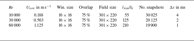


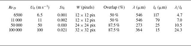
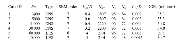


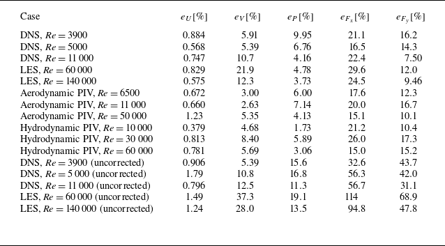


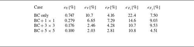


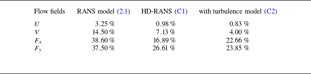


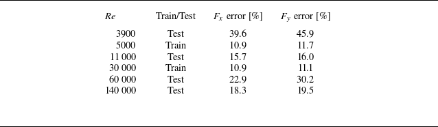


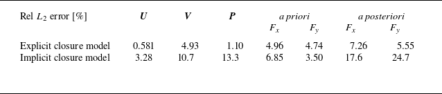


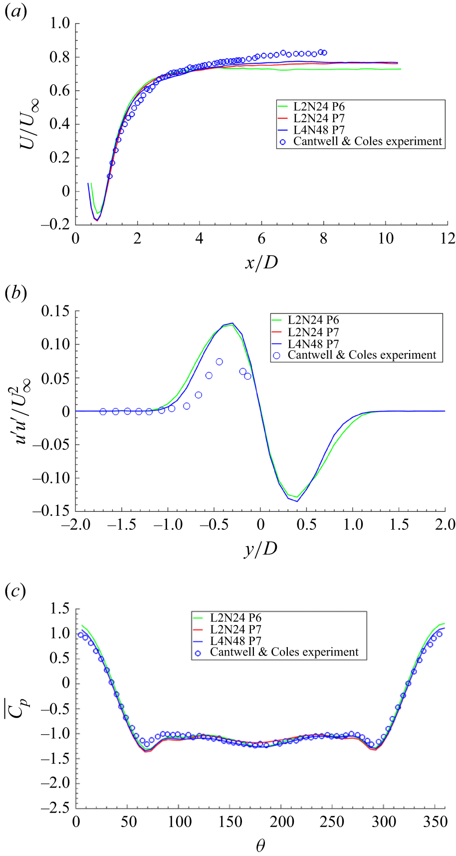


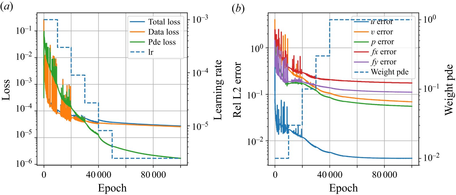


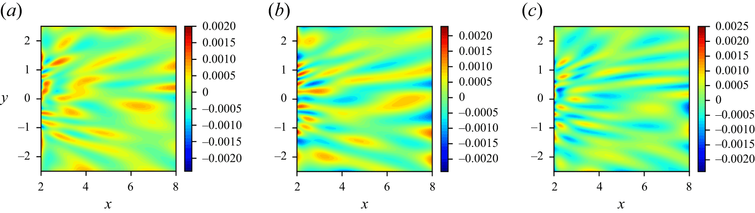

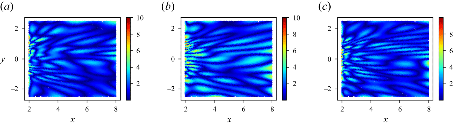


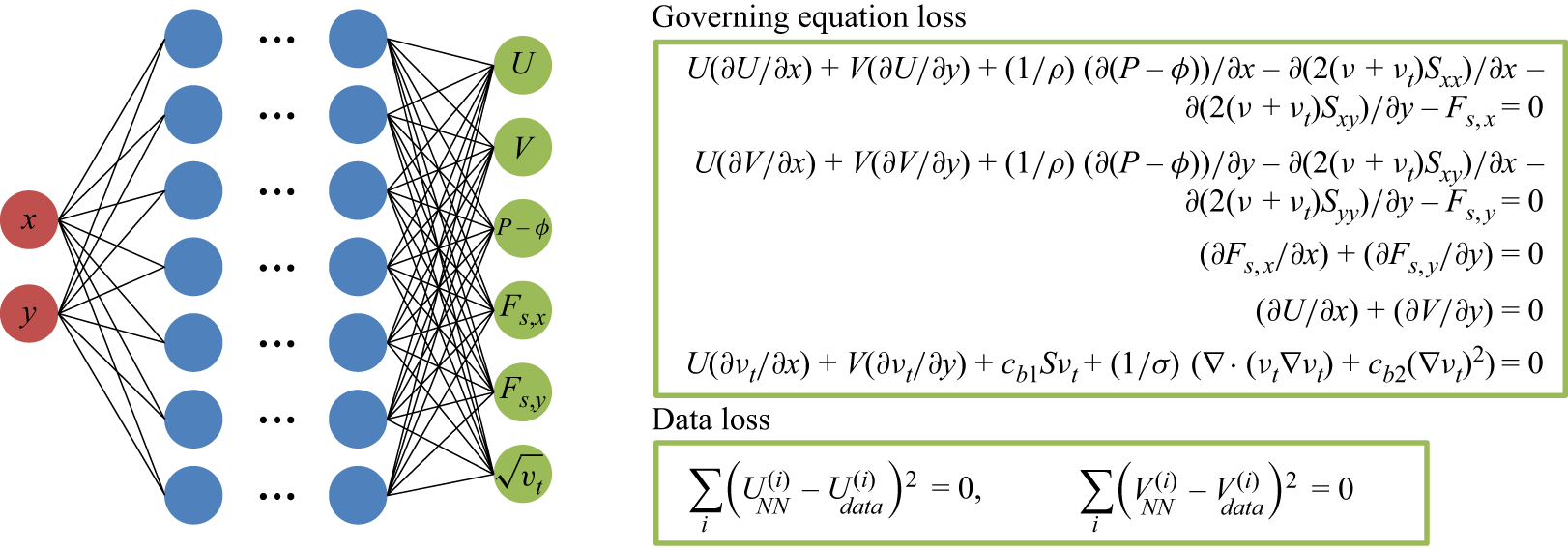
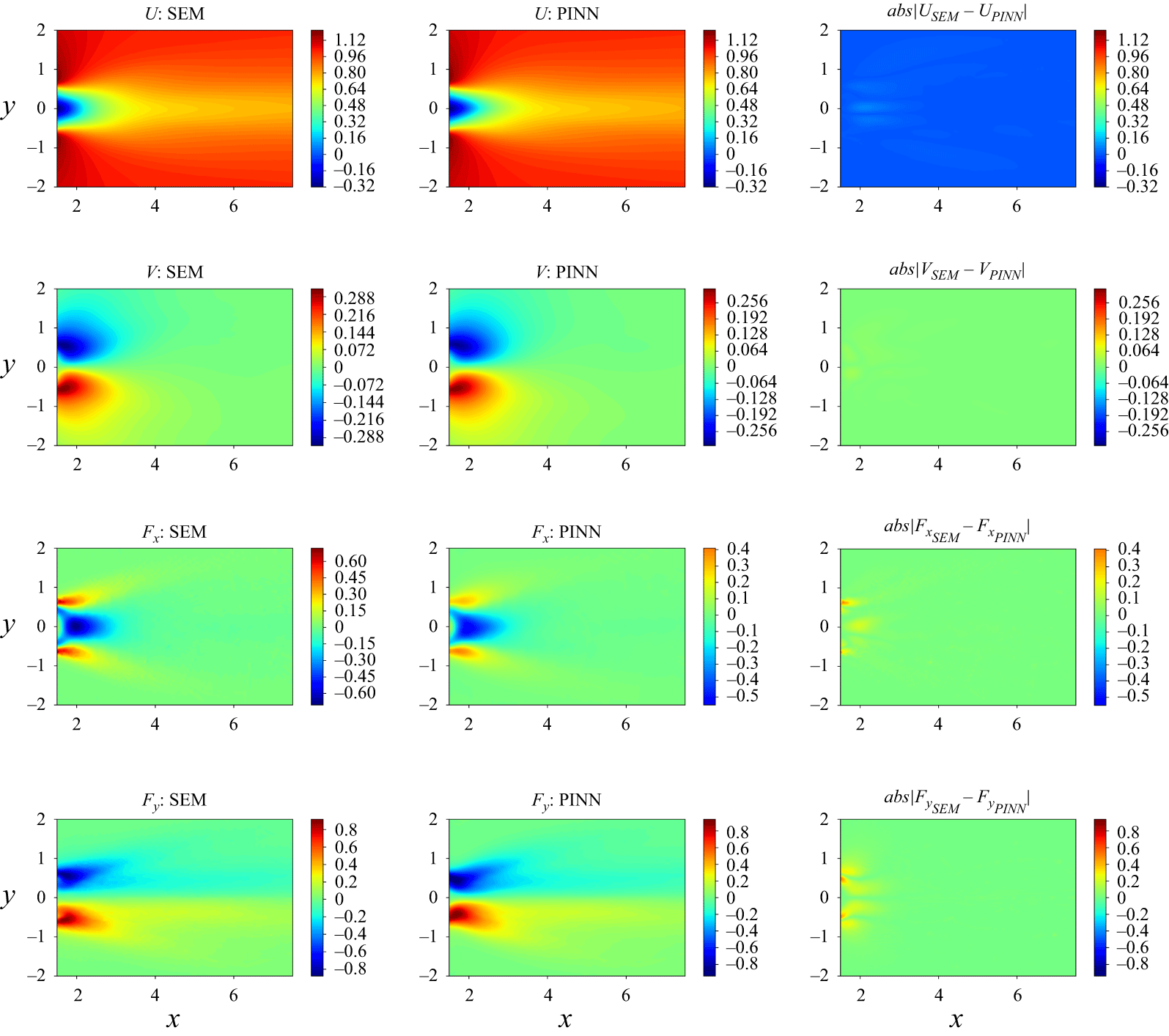


 Open access

