


I. Introduction
Researchers have found that debt is essential for funding innovations across diverse contexts, including publicly traded companies (Mann (Reference Mann2018)) and startups (Robb and Robinson (Reference Robb and Robinson2014), Davis, Morse, and Wang (Reference Davis, Morse and Wang2020)). Furthermore, empirical studies have shown that debt fosters innovation and that improved debt financing accelerates innovation and cultivates innovation novelty for firms (Benfratello, Schiantarelli, and Sembenelli (Reference Benfratello, Schiantarelli and Sembenelli2008), Amore, Schneider, and Žaldokas (Reference Amore, Schneider and Žaldokas2013), and Chava, Oettl, Subramanian, and Subramanian (Reference Chava, Oettl, Subramanian and Subramanian2013)), whereas credit market disruptions hinder innovation (Hombert and Matray (Reference Hombert and Matray2017), Granja and Moreira (Reference Granja and Moreira2023)).
This body of empirical evidence presents a puzzle in light of the conventional view that debt may not be desirable for financing innovation. Early work argues that debt contracts might not be well-suited for financing innovation due to the uncertainty surrounding research and development (R&D) outcomes, which can lead to credit rationing and premature liquidation (Stiglitz (Reference Stiglitz1985), Atanassov, Nanda, and Seru (Reference Atanassov, Nanda and Seru2007)). For practitioners engaged in innovation and its financing, however, it is crucial to distinguish between uncertainty (or ambiguity) and risk. The significant asymmetry of innovation payoffs further poses challenges to aligning fixed-obligation debt with innovation incentives (Manso (Reference Manso2011)). In addition, the intangible nature of R&D constrains collateral value and reduces the debt capacity of innovative firms (Hall and Lerner (Reference Hall, Lerner, Hall and Rosenberg2010)). Lastly, why debt can foster innovation remains an open question.
To address this question, we integrate the distinctive features of innovation returns into a framework for financing a growth option, originally developed by Sundaresan and Wang (Reference Sundaresan and Wang2007) and Sundaresan, Wang, and Yang (Reference Sundaresan, Wang and Yang2015). We distinguish risk—characterized by a single known probability distribution—from ambiguity, which is characterized by model uncertainty represented by a set of plausible distributions. In our setting, an entrepreneur makes joint decisions regarding when to initiate an innovation project and how to finance it. Once launched, the project generates cash flows characterized by both jumps and ambiguity—key features of innovation returns that distinguish them from conventional investments, as highlighted by Kerr, Nanda, and Rhodes-Kropf (Reference Kerr, Nanda and Rhodes-Kropf2014) and Kerr and Nanda (Reference Kerr and Nanda2015). While jumps are intrinsic to the cash flow dynamics under the objective measure, ambiguity reflects the entrepreneur’s subjective beliefs (Seo (Reference Seo2009), Baillon, Huang, Selim, and Wakker (Reference Baillon, Huang, Selim and Wakker2018)). The entrepreneur can finance the project either entirely with equity (all-equity financing) or with an optimal mix of equity and debt (optimal financing), the latter leveraging the tax benefits of debt while accounting for bankruptcy costs. Both the entrepreneur and external financiers are ambiguity-averse, making decisions under worst-case scenarios.
Our model highlights the central role of debt in fostering innovation through an investment acceleration mechanism. This mechanism emerges from the dynamic interaction between optimal investment timing, capital structure, and cash flow uncertainty. Under complete information, our model jointly and endogenously determines financing and investment decisions in a first-best equilibrium, without relying on exogenous financing constraints.
To ensure analytical tractability, we model innovation cash flows using the double-exponential jump diffusion process introduced by Kou (Reference Kou2002). This process not only captures the leptokurtic features commonly observed in asset and innovation returns but also allows for a closed-form characterization of the first-passage time distribution. Since both the investment and default options are path-dependent and their values hinge critically on first-passage probabilities, this tractability offers a distinct advantage over alternative jump-size specifications.
We extend the original recursive multiple priors utility (RMPU) framework developed by Chen and Epstein (Reference Chen and Epstein2002) to incorporate both diffusion and jump ambiguity. In the RMPU framework, agents possess a set of equivalent priors (probability measures) characterized by Itô diffusions and maximize utility under the worst-case prior. The state process under an alternative prior differs only in its drift, thereby altering the first moment only. However, this framework falls short when analyzing innovation as a driving force behind investment and financing choices, because diffusion increments are symmetric and normally distributed.
In this pursuit, we build on the mathematical framework of Quenez and Sulem (Reference Quenez and Sulem2013), (Reference Quenez and Sulem2014) to model agents’ multiple priors on innovation-driven cash flows as a set of equivalent Lévy processes. Under both drift and jump ambiguity, the density generator for an alternative prior consists of two components: one for Brownian risk and another for the Poisson random measure. Under jump ambiguity, the state process deviates from the reference measure not just in the mean but across the entire distribution. Solving the optimal stopping problem under such conditions is analytically challenging, particularly in determining the worst-case measure. To address this, we apply the theories of backward stochastic differential equations (BSDEs) with jumps (Quenez and Sulem (Reference Quenez and Sulem2013), (Reference Quenez and Sulem2014)) to derive the worst-case measure and closed-form solutions for optimal investment and financing decisions.
We use detection-error probabilities to calibrate ambiguity and compute relative entropy growth to quantify the contributions of diffusion ambiguity and jump ambiguity, building on Anderson, Hansen, and Sargent (Reference Anderson, Hansen and Sargent2003), Maenhout (Reference Maenhout2006), and Aït-Sahalia and Matthys (Reference Aït-Sahalia and Matthys2019). Under ambiguity, the worst-case measure is considered reasonable when it is statistically difficult to distinguish from the reference measure. Relative entropy growth measures the statistical distance between two priors. In the model, the total relative entropy growth is comprised of two additive components driven by diffusion and jump ambiguity. In the context of innovation, it is important to examine the influence of the two types of ambiguity. For instance, in high-tech sectors where innovations often exhibit radical characteristics, the role of jump ambiguity is naturally magnified, whereas traditional sectors are expected to show the opposite feature.
We show that the investment acceleration benefit of debt for project value arises from the interaction between two effects: the reduction in the investment threshold and the passage time effect—the time it takes for cash flows to reach a target level from below. Under optimal financing, firms invest at a lower cash flow level rather than waiting to reach the higher threshold required under all-equity financing, as the net tax benefit of debt offsets the difference.Footnote 1 This lower threshold leads to earlier investment in expectation, thereby increasing the project’s expected net present value. Moreover, we demonstrate that the passage time effect amplifies this value gain in a power-law fashion.
Innovation projects, which typically involve greater ambiguity, benefit more from the investment acceleration effect of debt. Although ambiguity raises the investment thresholds, delays investment, and lowers project values under both financing scenarios, optimal financing mitigates these adverse effects.Footnote 2 On one hand, ambiguity reduces optimal leverage and hence the net tax benefit of debt, narrowing the threshold gap between optimal and all-equity financing. Nevertheless, this gap shrinks at a diminishing rate. On the other hand, ambiguity strengthens the passage time effect by further delaying investment under all-equity financing. The combination of a slowly declining threshold gap and an increasingly dominant power effect explains why the investment acceleration benefit of debt is amplified under greater ambiguity.
Moreover, our analysis reveals that the fostering effect of debt is particularly pronounced when innovative firms have limited historical data for gauging ambiguity. This result helps explain why young startups, which typically lack extensive track records, often favor debt financing. This observation is consistent with empirical evidence from Robb and Robinson (Reference Robb and Robinson2014), Davis et al. (Reference Davis, Morse and Wang2020), and Chava et al. (Reference Chava, Oettl, Subramanian and Subramanian2013). Additionally, we find that the fostering effect of debt is especially significant for radical innovations when jump ambiguity is the primary concern. This finding aligns with Benfratello et al. (Reference Benfratello, Schiantarelli and Sembenelli2008), who show that high-tech firms benefit greatly from increased credit availability, given their focus on radical innovations capable of generating substantial jumps in returns.
Our theoretical results on the elevated investment threshold and reduced project scale under ambiguity contribute to the broader literature on investment under uncertainty, pioneered by Bloom (Reference Bloom2009).Footnote 3 Recent studies, including Gulen and Ion (Reference Gulen and Ion2016) and Campello, Cortes, d’Almeida, and Kankanhalli (Reference Campello, Cortes, d’Almeida and Kankanhalli2022), document that heightened economic policy uncertainty suppresses corporate investment. As recent research (e.g., Aït-Sahalia, Matthys, Osambela, and Sircar (Reference Aït-Sahalia, Matthys, Osambela and Sircar2025)) uses the economic policy uncertainty index as a proxy for ambiguity, these findings align well with the prediction of our model that ambiguity delays investment. In addition, our result that greater ambiguity leads to smaller optimal project scales echoes the findings of Campello, Kankanhalli, and Kim (Reference Campello, Kankanhalli and Kim2024), who show that firms respond to elevated uncertainty by delaying both investment and disinvestment, particularly when sunk costs are high. Taken together, these empirical patterns reinforce our theoretical insight that ambiguity discourages large-scale commitments in uncertain environments.
Existing real option models focus on diffusion ambiguity only, for example, see Nishimura and Ozaki (Reference Nishimura and Ozaki2007) and Miao and Wang (Reference Miao and Wang2011). These models do not consider jump ambiguity, nor do they investigate financing choices, as we do in our paper. Dicks and Fulghieri (Reference Dicks and Fulghieri2021) develop a theory of innovation waves and investor sentiment tied to ambiguity. Coiculescu, Izhakian, and Ravid (Reference Coiculescu, Izhakian and Ravid2024) treat innovation as real options and find that ambiguity negatively impacts R&D, while risk has a positive effect. A recent and closely related study by Geelen, Hajda, and Morellec (Reference Geelen, Hajda and Morellec2022) develops a Schumpeterian growth model with endogenous R&D and financing choices, demonstrating that debt fosters innovation and growth at the aggregate level, similar to our findings. They attribute this effect to the tax benefit of debt. Different from this study, our model emphasizes the interaction between debt financing and jump ambiguity, a defining feature of innovation returns.
II. The Model
Our baseline model combines the irreversible investment framework of McDonald and Siegel (Reference McDonald and Siegel1986) with the EBIT-based capital structure model of Goldstein, Ju, and Leland (Reference Goldstein, Ju and Leland2001). Sundaresan and Wang (Reference Sundaresan and Wang2007) and Sundaresan et al. (Reference Sundaresan, Wang and Yang2015) formally analyze the joint implications of these models and extend them further. We adopt their assumptions but introduce jump risk into the baseline model. Our main contribution is to examine the effects of ambiguity about both the drift and the jump intensity and size distribution.
A. The Baseline Model without Ambiguity
1. The Project
An entrepreneur has access to an innovation project that, once initiated, generates an earnings before interest and taxes (EBIT) flow $ X(t):= X\left(t,\omega \right) $
defined on a probability space (
$ X(t):= X\left(t,\omega \right) $
defined on a probability space ( $ \Omega, \mathcal{F},{Q}^0) $
endowed with a standard complete filtration
$ \Omega, \mathcal{F},{Q}^0) $
endowed with a standard complete filtration $ \mathbf{F}=\{{\mathcal{F}}_t|t\ge 0\} $
satisfying the “usual conditions.” We assume that the EBIT process is exogenous and independent of the entrepreneur’s investment decision. We specify
$ \mathbf{F}=\{{\mathcal{F}}_t|t\ge 0\} $
satisfying the “usual conditions.” We assume that the EBIT process is exogenous and independent of the entrepreneur’s investment decision. We specify $ {Q}^0 $
to be the risk-neutral probability measure, in line with the traditional EBIT-based capital structure model of Goldstein et al. (Reference Goldstein, Ju and Leland2001).Footnote 4 Under
$ {Q}^0 $
to be the risk-neutral probability measure, in line with the traditional EBIT-based capital structure model of Goldstein et al. (Reference Goldstein, Ju and Leland2001).Footnote 4 Under $ {Q}^0 $
,
$ {Q}^0 $
, $ X(t) $
follows a geometric Lévy process:
$ X(t) $
follows a geometric Lévy process:
 $$ \frac{dX(t)}{X\left({t}^{-}\right)}=\mu dt+\sigma dW(t)+{\int}_{\mathrm{\mathbb{R}}}\iota \left(t,u\right)\tilde{N}\left( dt, du\right), $$
where $ W(t) $
is a standard Brownian motion,
$ W(t) $
is a standard Brownian motion, $ \tilde{N}\left( dt, du\right) $
is a compensated Poisson random measure given by
$ \tilde{N}\left( dt, du\right) $
is a compensated Poisson random measure given by
 $$ \tilde{N}\left( dt, du\right)=N\left( dt, du\right)-\nu (du) dt, $$
with $ \nu (du):= \unicode{x1D53C}\left[N\left(1, du\right)\right] $
being the Lévy measure, and
$ \nu (du):= \unicode{x1D53C}\left[N\left(1, du\right)\right] $
being the Lévy measure, and $ \iota \left(t,u\right) $
being a square-integrable predictable process with respect to
$ \iota \left(t,u\right) $
being a square-integrable predictable process with respect to $ \nu (du) $
. It is worth noting that the specification of a compensated Poisson random measure under the risk-neutral reference measure follows the same rational expectation equilibrium pricing rule as in Goldstein et al. (Reference Goldstein, Ju and Leland2001).Footnote 5 Additionally, we assume that
$ \nu (du) $
. It is worth noting that the specification of a compensated Poisson random measure under the risk-neutral reference measure follows the same rational expectation equilibrium pricing rule as in Goldstein et al. (Reference Goldstein, Ju and Leland2001).Footnote 5 Additionally, we assume that $ X(0)=x>0 $
,
$ X(0)=x>0 $
, $ \mu $
,
$ \mu $
, $ \sigma $
, and
$ \sigma $
, and $ r $
are constants with
$ r $
are constants with $ \mu <r $
and
$ \mu <r $
and $ r $
being the risk-free rate.
$ r $
being the risk-free rate.
We specify the jump component as a compound Poisson process with intensity $ \lambda <+\infty $
and assume a double exponential distribution for the jump size (i.e.,
$ \lambda <+\infty $
and assume a double exponential distribution for the jump size (i.e., $ X(t) $
follows a double exponential jump-diffusion process, first introduced by Kou (Reference Kou2002)). Specifically, we can write the jump component explicitly as
$ X(t) $
follows a double exponential jump-diffusion process, first introduced by Kou (Reference Kou2002)). Specifically, we can write the jump component explicitly as
 $$ \iota \left(t,u\right)={e}^u-1,\hskip1em \mathrm{and}\hskip1em \nu (du)=\lambda f(du), $$
where the jump size density $ f $
is given by
$ f $
is given by
 $$ {f}_u=p{\eta}_1{e}^{-{\eta}_1u}{\mathbf{1}}_{u\ge 0}+q{\eta}_2{e}^{\eta_2u}{\mathbf{1}}_{u<0},\hskip1em {\eta}_1>1,{\eta}_2>0,p,q\ge 0,p+q=1 $$
in which $ \mathbf{1} $
is an indicator function. In the specification,
$ \mathbf{1} $
is an indicator function. In the specification, $ p $
and
$ p $
and $ q $
are the conditional probabilities of upward and downward jumps, respectively, and
$ q $
are the conditional probabilities of upward and downward jumps, respectively, and $ 1/{\eta}_1 $
and
$ 1/{\eta}_1 $
and $ -1/{\eta}_2 $
are the conditional mean log jump sizes of positive and negative jumps, respectively. This model specification has two merits. First, as shown by Kou and Wang (Reference Kou and Wang2004), it allows for analytical solutions to valuation problems with American-style perpetual options.Footnote 6 This property is crucial to our analyses of joint investment and financing decisions in the real options model. Second, the specification has the appealing feature of modeling positive and negative jumps separately, which generates a rich set of priors, as will be shown later.
$ -1/{\eta}_2 $
are the conditional mean log jump sizes of positive and negative jumps, respectively. This model specification has two merits. First, as shown by Kou and Wang (Reference Kou and Wang2004), it allows for analytical solutions to valuation problems with American-style perpetual options.Footnote 6 This property is crucial to our analyses of joint investment and financing decisions in the real options model. Second, the specification has the appealing feature of modeling positive and negative jumps separately, which generates a rich set of priors, as will be shown later.
2. Financing
We assume that the project requires external funding, as available cash is insufficient. Taxation on project cash flows at rate $ \phi \in \left(0,1\right) $
motivates firms to issue debt for tax shielding. The entrepreneur chooses between all equity financing and optimal financing, aiming to determine the optimal equity-debt mix.Footnote 7 Drawing on the established literature (e.g., Leland (Reference Leland1998), Goldstein et al. (Reference Goldstein, Ju and Leland2001)), we analyze debt contracts with perpetual coupon payments
$ \phi \in \left(0,1\right) $
motivates firms to issue debt for tax shielding. The entrepreneur chooses between all equity financing and optimal financing, aiming to determine the optimal equity-debt mix.Footnote 7 Drawing on the established literature (e.g., Leland (Reference Leland1998), Goldstein et al. (Reference Goldstein, Ju and Leland2001)), we analyze debt contracts with perpetual coupon payments $ C $
in a time-homogeneous context. Debt issuance reduces tax by
$ C $
in a time-homogeneous context. Debt issuance reduces tax by $ \phi C $
but also exposes the firm to potential bankruptcy costs.
$ \phi C $
but also exposes the firm to potential bankruptcy costs.
We begin with the all-equity financing case. The equity value at the $ {\mathrm{\mathcal{F}}}_0 $
-measurable random investment time
$ {\mathrm{\mathcal{F}}}_0 $
-measurable random investment time $ {\tau}_I\ge 0 $
is
$ {\tau}_I\ge 0 $
is
 $$ {V}_e\left({\tau}_I\right)={\unicode{x1D53C}}_{\tau_I}\left[{\int}_{\tau_I}^{\infty }{e}^{-r\left(t-{\tau}_I\right)}\left(1-\phi \right)X(t) dt-I\right], $$
where the constant $ I>0 $
denotes the investment cost. At time 0, the entrepreneur chooses the optimal stopping time
$ I>0 $
denotes the investment cost. At time 0, the entrepreneur chooses the optimal stopping time $ {\tau}_I^e $
to initiate the project; hence, her value function at time 0 is
$ {\tau}_I^e $
to initiate the project; hence, her value function at time 0 is
 $$ {V}_e(0)=\underset{\tau_I}{\sup}\;{\unicode{x1D53C}}_0\left[{e}^{-r{\tau}_I}{V}_e\left({\tau}_I\right)\right]={\unicode{x1D53C}}_0\left[{e}^{-r{\tau}_I^e}{V}_e\left({\tau}_I^e\right)\right]. $$
In the case of optimal financing, the entrepreneur can issue debt at the time of investment, $ {\tau}_I $
, to take advantage of the tax benefits associated with debt. Default occurs later, at the stopping time
$ {\tau}_I $
, to take advantage of the tax benefits associated with debt. Default occurs later, at the stopping time $ {\tau}_D $
under the assumption of optimal default, a standard assumption in the literature (Sundaresan and Wang (Reference Sundaresan and Wang2007), Strebulaev and Whited (Reference Strebulaev and Whited2012), and Sundaresan et al. (Reference Sundaresan, Wang and Yang2015)). As per the traditional trade-off theory of capital structure (e.g., Leland (Reference Leland1994), Goldstein et al. (Reference Goldstein, Ju and Leland2001)), default triggers liquidation under the absolute priority rule, with a fraction
$ {\tau}_D $
under the assumption of optimal default, a standard assumption in the literature (Sundaresan and Wang (Reference Sundaresan and Wang2007), Strebulaev and Whited (Reference Strebulaev and Whited2012), and Sundaresan et al. (Reference Sundaresan, Wang and Yang2015)). As per the traditional trade-off theory of capital structure (e.g., Leland (Reference Leland1994), Goldstein et al. (Reference Goldstein, Ju and Leland2001)), default triggers liquidation under the absolute priority rule, with a fraction $ \alpha \in \left(0,1\right) $
of the asset value lost in the liquidation process. This assumption is standard in models that balance the benefits of debt (via tax shields) with the costs of potential default and liquidation. Figure 1 illustrates the timelines for both financing choices.
$ \alpha \in \left(0,1\right) $
of the asset value lost in the liquidation process. This assumption is standard in models that balance the benefits of debt (via tax shields) with the costs of potential default and liquidation. Figure 1 illustrates the timelines for both financing choices.
The timeline in Figure 1 illustrates the investment option and potential default under debt financing.

Given the above, the firm value at the investment time $ {\tau}_I $
is
$ {\tau}_I $
is
 $$ {V}_{\ast}\left({\tau}_I\right)=E\left({\tau}_I\right)+D\left({\tau}_I\right)-I, $$
where $ D\left({\tau}_I\right) $
is the entrepreneur’s valuation of debt, and
$ D\left({\tau}_I\right) $
is the entrepreneur’s valuation of debt, and $ E\left({\tau}_I\right) $
is the value of (leveraged) equity, given by
$ E\left({\tau}_I\right) $
is the value of (leveraged) equity, given by
 $$ {\displaystyle \begin{array}{c}E\left({\tau}_I\right)=\underset{\tau_D\ge {\tau}_I}{\sup}\;{\unicode{x1D53C}}_{\tau_I}\left[{\int}_{\tau_I}^{\tau_D}{e}^{-r\left(t-{\tau}_I\right)}\left(1-\phi \right)\left(X(t)-C\right) dt\right]\\ {}={\unicode{x1D53C}}_{\tau_I}\left[{\int}_{\tau_I}^{\tau_D^{\ast }}{e}^{-r\left(t-{\tau}_I\right)}\left(1-\phi \right)\left(X(t)-C\right) dt\right].\end{array}} $$
The above indicates that the equity value is the discounted net profit received by equity holders until default. At default, equity holders recover nothing. As is standard in the trade-off theory of capital structure, we assume that the entrepreneur maximizes equity value by choosing the default policy $ {\tau}_D $
. However, when choosing the optimal debt policy
$ {\tau}_D $
. However, when choosing the optimal debt policy $ {C}^{\ast } $
, she maximizes firm value
$ {C}^{\ast } $
, she maximizes firm value $ {V}_{\ast}\left({\tau}_I\right) $
, incorporating her expectation of debt value
$ {V}_{\ast}\left({\tau}_I\right) $
, incorporating her expectation of debt value $ D\left({\tau}_I\right) $
.Footnote 8 In a symmetric rational expectation equilibrium, the entrepreneur’s valuation of debt,
$ D\left({\tau}_I\right) $
.Footnote 8 In a symmetric rational expectation equilibrium, the entrepreneur’s valuation of debt, $ D\left({\tau}_I\right) $
, equals debt investors’ valuation and is given by
$ D\left({\tau}_I\right) $
, equals debt investors’ valuation and is given by
 $$ D\left({\tau}_I\right)={\unicode{x1D53C}}_{\tau_I}\left[{\int}_{\tau_I}^{\tau_D^{\ast }}{e}^{-r\left(t-{\tau}_I\right)} Cdt+\left(1-\alpha \right){\int}_{\tau_D^{\ast}}^{\infty }{e}^{-r\left(t-{\tau}_I\right)}\left(1-\phi \right)X(t) dt\right]. $$
The first term inside the conditional expectation operator is the present value of the coupon collected while the firm remains solvent. The second term is the present value of the asset value recovered upon liquidation in bankruptcy.
Since $ {\tau}_D^{\ast } $
and
$ {\tau}_D^{\ast } $
and $ {C}^{\ast } $
depend on
$ {C}^{\ast } $
depend on $ {\tau}_I^{\ast } $
, these three decision variables are jointly determined at time 0 by maximizing the discounted firm value at investment.
$ {\tau}_I^{\ast } $
, these three decision variables are jointly determined at time 0 by maximizing the discounted firm value at investment.
 $$ {V}_{\ast }(0)=\underset{\tau_I,{\tau}_D>{\tau}_I,C}{\sup}\;{\unicode{x1D53C}}_0\left[{e}^{-r{\tau}_I}{V}_{\ast}\left({\tau}_I\right)\right]=\underset{\tau_I,{\tau}_D>{\tau}_I,C}{\sup}\;{\unicode{x1D53C}}_0\left[{e}^{-r{\tau}_I}{\unicode{x1D53C}}_{\tau_I}\left[{V}_{\ast}\left({\tau}_I\right)\right]\right], $$
where the second equality follows from the property of conditional expectations, and the optimization is subject to the default policy determined in (4).
B. The Set of Priors
Agents face ambiguity about the EBIT reference model in equation (1) and consider “close” alternative models. With ambiguity aversion, they opt for worst-case EBIT dynamics. To capture jump ambiguity, we extend the utility framework of Chen and Epstein (Reference Chen and Epstein2002) to allow for uncertainty in both jump intensity and size distribution. Our extension builds on the general results of Quenez and Sulem (Reference Quenez and Sulem2013), (Reference Quenez and Sulem2014), who provide the comparison theorem for BSDEs under Lévy processes and general results for related optimal stopping problems under ambiguity.
Let $ \Theta $
denote the set of density generators. Each density generator
$ \Theta $
denote the set of density generators. Each density generator $ \theta \in \Theta $
is binary (i.e.,
$ \theta \in \Theta $
is binary (i.e., $ \theta =\left({\theta}_W,{\theta}_N\right) $
, where
$ \theta =\left({\theta}_W,{\theta}_N\right) $
, where $ {\theta}_W $
is for the Brownian motion and
$ {\theta}_W $
is for the Brownian motion and $ {\theta}_N $
for the jump component). For each
$ {\theta}_N $
for the jump component). For each $ \theta \in \Theta $
, let
$ \theta \in \Theta $
, let $ {Z}^{\theta }(t) $
be the solution to the (forward) SDE:
$ {Z}^{\theta }(t) $
be the solution to the (forward) SDE:
 $$ {dZ}^{\theta }(t)={Z}^{\theta}\left({t}^{-}\right)\left(-{\theta}_W(t) dW(t)-{\int}_{\mathrm{\mathbb{R}}}{\theta}_N\Big(t,u\Big)d\tilde{N}( dt, du\Big)\right), $$
for $ t\in \left[0,T\right] $
with
$ t\in \left[0,T\right] $
with $ {Z}^{\theta }(0)=1 $
. For
$ {Z}^{\theta }(0)=1 $
. For $ {\theta}_W(t) $
, we adopt the
$ {\theta}_W(t) $
, we adopt the $ \kappa $
-ignorance specification of Chen and Epstein (Reference Chen and Epstein2002) (i.e.,
$ \kappa $
-ignorance specification of Chen and Epstein (Reference Chen and Epstein2002) (i.e., $ {\theta}_W(t)\in \left[-\kappa, \kappa \right],0<\kappa <\infty $
). Based on the technical requirements in Quenez and Sulem (Reference Quenez and Sulem2013), (Reference Quenez and Sulem2014), we specify
$ {\theta}_W(t)\in \left[-\kappa, \kappa \right],0<\kappa <\infty $
). Based on the technical requirements in Quenez and Sulem (Reference Quenez and Sulem2013), (Reference Quenez and Sulem2014), we specify $ {\theta}_N\left(t,u\right) $
as:
$ {\theta}_N\left(t,u\right) $
as:
 $$ {\displaystyle \begin{array}{ll}& {\theta}_N\left(t,u\right)=1-{e}^{\theta_{N,1}(t)u}{\mathbf{1}}_{u\ge 0}-{e}^{\theta_{N,2}(t)u}{\mathbf{1}}_{u<0},\\ {}& {\theta}_{N,1}(t)\in \left[-{M}_1,0\right],\hskip1em {\theta}_{N,2}(t)\in \left[0,{M}_2\right],\hskip1em \mathrm{and}\hskip1em {M}_1,{M}_2>0.\end{array}} $$
This specification for $ {\theta}_N\left(t,u\right) $
follows from the jump-size distribution in equation (2), and we discuss its implications after constructing the set of priors.
$ {\theta}_N\left(t,u\right) $
follows from the jump-size distribution in equation (2), and we discuss its implications after constructing the set of priors.
To construct the set of priors, we define a probability measure $ {Q}^{\theta } $
on
$ {Q}^{\theta } $
on $ {\mathrm{\mathcal{F}}}_T $
, equivalent to
$ {\mathrm{\mathcal{F}}}_T $
, equivalent to $ {Q}^0 $
for
$ {Q}^0 $
for $ \theta \in \Theta $
as
$ \theta \in \Theta $
as
 $$ {\unicode{x1D53C}}^{\theta}\left[{\mathbf{1}}_A\right]=\unicode{x1D53C}\left[{\mathbf{1}}_A{Z}_T^{\theta}\right],\hskip1em A\in {\mathrm{\mathcal{F}}}_T. $$
Hence, under $ {Q}^{\theta } $
,
$ {Q}^{\theta } $
,
 $$ {dW}^{\theta }(t)= dW(t)+{\theta}_W(t) dt, $$
which represents the Brownian risk, and
 $$ {\tilde{N}}^{\theta}\left( dt, du\right)=\tilde{N}\left( dt, du\right)+{\theta}_N\left(t,u\right)\nu (du) dt=N\left( dt, du\right)-\left(1-{\theta}_N\left(t,u\right)\right)\nu (du) dt, $$
which is a compensated Poisson random measure by Girsanov’s theorem; see Øksendal and Sulem ((Reference Øksendal and Sulem2019), Chapter 1.4). Taken together, under $ {Q}^{\theta } $
,
$ {Q}^{\theta } $
, $ X(t) $
is given by
$ X(t) $
is given by
 $$ \frac{dX(t)}{X\left({t}^{-}\right)}={\displaystyle \begin{array}{l}\left(\mu -{\theta}_W(t)\sigma -{\int}_{\mathrm{\mathbb{R}}}\left({e}^u-1\right){\theta}_N\left(t,u\right)\nu (du)\right) dt+\sigma {dW}^{\theta }(t)\\ {}+\hskip2px {\int}_{\mathrm{\mathbb{R}}}\left({e}^u-1\right){\tilde{N}}^{\theta}\left( dt, du\right).\end{array}} $$
Our method of distorting the reference measure can attenuate the impact of positive or negative jumps, depending on the monotonicity of the entrepreneur’s value function in the state variable. If the value function increases with the state variable, as in the baseline model without ambiguity, the worst-case measure leads to the smallest unconditional probability and mean size for positive jumps, and the largest values for negative jumps—all constrained within the set of priors. To see this, equation (5) shows that $ {N}^{\theta}\left( dt, du\right) $
has a Lévy measure
$ {N}^{\theta}\left( dt, du\right) $
has a Lévy measure $ {\nu}^{\theta }(du)=\left(1-{\theta}_N\left(t,u\right)\right)\nu (du) $
under
$ {\nu}^{\theta }(du)=\left(1-{\theta}_N\left(t,u\right)\right)\nu (du) $
under $ {Q}^{\theta } $
. We can express
$ {Q}^{\theta } $
. We can express $ {\nu}^{\theta }(du) $
as
$ {\nu}^{\theta }(du) $
as
 $$ {\nu}^{\theta }(du)={\lambda}_t^{\theta }{f}_t^{\theta }(du), $$
where $ {\lambda}_t^{\theta } $
is the distorted jump intensity given by
$ {\lambda}_t^{\theta } $
is the distorted jump intensity given by
 $$ {\lambda}_t^{\theta }=\lambda {\int}_{\mathrm{\mathbb{R}}}\left(1-{\theta}_N\left(t,u\right)\right){f}_u du=\lambda \left(\frac{p{\eta}_1}{\eta_1-{\theta}_{N,1}(t)}+\frac{q{\eta}_2}{\eta_2+{\theta}_{N,2}(t)}\right), $$
and the distorted jump size density is given by
 $$ {\displaystyle \begin{array}{c}{f}_{u,t}^{\theta }=\frac{\left(1-{\theta}_N\left(t,u\right)\right){f}_u}{\int_{\mathrm{\mathbb{R}}}\left(1-{\theta}_N\left(t,u\right)\right){f}_u du}\\ {}={p}_t^{\theta}\left({\eta}_1-{\theta}_{N,1}(t)\right){e}^{-\left({\eta}_1-{\theta}_{N,1}(t)\right)u}{\mathbf{1}}_{u\ge 0}+{q}_t^{\theta}\left({\eta}_2+{\theta}_{N,2}(t)\right){e}^{\left({\eta}_2+{\theta}_{N,2}(t)\right)u}{\mathbf{1}}_{u<0},\end{array}} $$
with $ {p}_t^{\theta } $
and
$ {p}_t^{\theta } $
and $ {q}_t^{\theta } $
being the distorted probabilities of upward and downward jumps given by
$ {q}_t^{\theta } $
being the distorted probabilities of upward and downward jumps given by
 $$ {\displaystyle \begin{array}{l}{p}_t^{\theta }=\frac{p{\eta}_1\left({\eta}_2+{\theta}_{N,2}(t)\right)}{p{\eta}_1\left({\eta}_2+{\theta}_{N,2}(t)\right)+q{\eta}_2\left({\eta}_1-{\theta}_{N,1}(t)\right)},\ \mathrm{and}\\ {}{q}_t^{\theta }=\frac{q{\eta}_2\left({\eta}_1-{\theta}_{N,1}(t)\right)}{p{\eta}_1\left({\eta}_2+{\theta}_{N,2}(t)\right)+q{\eta}_2\left({\eta}_1-{\theta}_{N,1}(t)\right)}.\end{array}} $$
Table 1 summarizes the Lévy measures for $ {N}^{\theta}\left( dt, du\right) $
under the set of priors specified
$ {N}^{\theta}\left( dt, du\right) $
under the set of priors specified $ {\theta}_{N,1}(t)\in \left[-{M}_1,0\right] $
and
$ {\theta}_{N,1}(t)\in \left[-{M}_1,0\right] $
and $ {\theta}_{N,2}(t)\in \left[0,{M}_2\right] $
. In the extreme case where only positive jumps occur (
$ {\theta}_{N,2}(t)\in \left[0,{M}_2\right] $
. In the extreme case where only positive jumps occur ( $ p=1 $
), the jump intensity ranges from
$ p=1 $
), the jump intensity ranges from $ \left[{\lambda \eta}_1/\left({\eta}_1+{M}_1\right),\lambda \right] $
, with the conditional probability of positive jumps fixed at 1. If the worst-case scenario corresponds to
$ \left[{\lambda \eta}_1/\left({\eta}_1+{M}_1\right),\lambda \right] $
, with the conditional probability of positive jumps fixed at 1. If the worst-case scenario corresponds to $ {\theta}_{N,1}(t)=-{M}_1 $
(or 0) for all
$ {\theta}_{N,1}(t)=-{M}_1 $
(or 0) for all $ t\ge 0 $
, the jump intensity is minimized (or maximized). A similar observation holds for the other extreme case (
$ t\ge 0 $
, the jump intensity is minimized (or maximized). A similar observation holds for the other extreme case ( $ q=1 $
).
$ q=1 $
).

C. Innovation with All-Equity Financing under Ambiguity
With the set of priors, the entrepreneur’s value function under all-equity financing at the investment time $ {\tau}_I $
and under a candidate measure
$ {\tau}_I $
and under a candidate measure $ {Q}^{\theta } $
is
$ {Q}^{\theta } $
is
 $$ {V}_e\left({\tau}_I;\theta \right)={\unicode{x1D53C}}_{\tau_I}^{\theta}\left[{\int}_{\tau_I}^{\infty }{e}^{-r\left(t-{\tau}_I\right)}\left(1-\phi \right)X(t) dt-I\right]. $$
At time 0, she chooses the optimal investment time $ {\tau}_I^e $
to start the project. The ambiguity-averse entrepreneur chooses the worst-case measure
$ {\tau}_I^e $
to start the project. The ambiguity-averse entrepreneur chooses the worst-case measure $ {Q}^{\theta^{\ast }} $
from the set of priors. As long as
$ {Q}^{\theta^{\ast }} $
from the set of priors. As long as $ {Q}^{\theta^e}\left\{{\tau}_I^{\ast }<+\infty \right\}=1 $
, her value function at time 0 is
$ {Q}^{\theta^e}\left\{{\tau}_I^{\ast }<+\infty \right\}=1 $
, her value function at time 0 is
 $$ {V}_e\left(0;{\tau}_I^e,{\theta}^{\ast}\right)=\underset{\tau_I\ge 0}{\sup}\;\underset{Q^{\theta }}{\operatorname{inf}}\;{\unicode{x1D53C}}_0^{\theta}\left[{e}^{-r{\tau}_I}{V}_e\left({\tau}_I;\theta \right)\right]. $$
It is necessary to discuss a few technical details of the optimal stopping problem under ambiguity, given by equations (6) and (7). First, Quenez and Sulem (Reference Quenez and Sulem2014) prove that the nonlinear expectation in (7) admits the minmax relation. Thus, we can first solve the minimum expectation problem to find the worst-case measure $ {Q}^{\theta^{\ast }} $
and then solve the optimal stopping problem for
$ {Q}^{\theta^{\ast }} $
and then solve the optimal stopping problem for $ {\tau}_I^{\ast } $
under
$ {\tau}_I^{\ast } $
under $ {Q}^{\theta^{\ast }} $
. Because the minimum expectation problem involves the application of Girsanov’s theorem and the comparison theorem for BSDEs under Lévy processes and because
$ {Q}^{\theta^{\ast }} $
. Because the minimum expectation problem involves the application of Girsanov’s theorem and the comparison theorem for BSDEs under Lévy processes and because $ {Q}^{\theta^{\ast }} $
exists for any horizon in our model, we can solve the optimal stopping problem under
$ {Q}^{\theta^{\ast }} $
exists for any horizon in our model, we can solve the optimal stopping problem under $ {Q}^{\theta^{\ast }} $
for the infinite horizon. Second, Quenez and Sulem (Reference Quenez and Sulem2013) show that the minimum expectation is dynamically consistent:
$ {Q}^{\theta^{\ast }} $
for the infinite horizon. Second, Quenez and Sulem (Reference Quenez and Sulem2013) show that the minimum expectation is dynamically consistent:
 $$ \underset{Q^{\theta }}{\operatorname{inf}}\;{\unicode{x1D53C}}_0^{\theta}\left[{e}^{-r{\tau}_I}{V}_e\left({\tau}_I;\theta \right)\right]=\underset{Q^{\theta^{\prime }}}{\operatorname{inf}}\;{\unicode{x1D53C}}_0^{\theta^{\prime }}\left[\underset{Q^{\theta^{{\prime\prime} }}}{\operatorname{inf}}\;{\unicode{x1D53C}}_{\tau_I}^{\theta^{{\prime\prime} }}\left[{e}^{-r{\tau}_I}{V}_e\left({\tau}_I;\left\{{\theta}^{\prime },{\theta}^{{\prime\prime}}\right\}\right)\right]\right]. $$
where $ {\theta}^{\prime } $
and
$ {\theta}^{\prime } $
and $ {\theta}^{{\prime\prime} } $
deliver density generators for the decision intervals
$ {\theta}^{{\prime\prime} } $
deliver density generators for the decision intervals $ \left[0,{\tau}_I\right] $
and
$ \left[0,{\tau}_I\right] $
and $ \left[{\tau}_I,T\right] $
with
$ \left[{\tau}_I,T\right] $
with $ T\le +\infty $
, respectively. Dynamic consistency provides analytical convenience in that the worst-case density generators for
$ T\le +\infty $
, respectively. Dynamic consistency provides analytical convenience in that the worst-case density generators for $ \left[0,{\tau}_I\right] $
and
$ \left[0,{\tau}_I\right] $
and $ \left[{\tau}_I,T\right] $
coincide with that for
$ \left[{\tau}_I,T\right] $
coincide with that for $ \left[0,T\right] $
. Hence, it suffices to begin with the following to find the worst-case measure:
$ \left[0,T\right] $
. Hence, it suffices to begin with the following to find the worst-case measure:
 $$ {V}_e\left(0;{\tau}_I,{\theta}^{\ast}\right)=\underset{Q^{\theta }}{\operatorname{inf}}\;{\unicode{x1D53C}}_0^{\theta}\left[{e}^{-r{\tau}_I}{V}_e\left({\tau}_I;\theta \right)\right],\hskip1em \mathrm{for}\hskip0.42em \mathrm{any}\hskip0.42em {\tau}_{\mathrm{I}}. $$
Proposition 1. The density generator that gives the minimum expectation in (8) is $ {\theta}^{\ast }=\left({\theta}_W^{\ast },{\theta}_N^{\ast}\right)=\left(\kappa, 1-{e}^{-{M}_1u}{\boldsymbol{1}}_{u\ge 0}-{\boldsymbol{1}}_{u<0}\right) $
for all
$ {\theta}^{\ast }=\left({\theta}_W^{\ast },{\theta}_N^{\ast}\right)=\left(\kappa, 1-{e}^{-{M}_1u}{\boldsymbol{1}}_{u\ge 0}-{\boldsymbol{1}}_{u<0}\right) $
for all $ t\in \left[0,T\right] $
.
$ t\in \left[0,T\right] $
.
In the Supplementary Material, we provide the proof, which relies on dynamic consistency and the comparison theorem for BSDEs under the Lévy process.
An immediate implication is that under $ {Q}^{\theta^{\ast }} $
,
$ {Q}^{\theta^{\ast }} $
, $ X(t) $
follows the process
$ X(t) $
follows the process
 $$ \frac{dX(t)}{X\left({t}^{-}\right)}={\mu}^{\theta^{\ast }} dt+\sigma {dW}^{\theta^{\ast }}(t)+{\int}_{\mathrm{\mathbb{R}}}\left({e}^u-1\right){\tilde{N}}^{\theta^{\ast }}\left( dt, du\right) $$
where
 $$ {\displaystyle \begin{array}{c}{\mu}^{\theta^{\ast }}=\mu -\kappa \sigma -{\int}_{\mathrm{\mathbb{R}}}\left({e}^u-1\right)\left(1-{e}^{-{M}_1u}{\mathbf{1}}_{u\ge 0}-{\mathbf{1}}_{u<0}\right)\nu (du)\\ {}=\mu +\underset{\mathrm{drift}\ \mathrm{ambiguity}\ \mathrm{discount}<0}{\underbrace{\left(-\kappa \sigma \right)}}+\underset{\mathrm{jump}\ \mathrm{ambiguity}\ \mathrm{discount}<0}{\underbrace{\left(-\frac{\lambda p}{\left({\eta}_1-1\right)}+\frac{\lambda p{\eta}_1}{\left({\eta}_1+{M}_1-1\right)\left({\eta}_1+{M}_1\right)}\right)}}.\end{array}} $$
The distorted process above indicates that drift ambiguity and jump ambiguity reduce the perceived mean return by $ \kappa \sigma $
and
$ \kappa \sigma $
and $ \lambda p/\left({\eta}_1-1\right)-\lambda p{\eta}_1/\left({\eta}_1+{M}_1-1\right)\left({\eta}_1+{M}_1\right) $
, respectively.
$ \lambda p/\left({\eta}_1-1\right)-\lambda p{\eta}_1/\left({\eta}_1+{M}_1-1\right)\left({\eta}_1+{M}_1\right) $
, respectively.
Before turning to the detailed discussion of $ X(t) $
under
$ X(t) $
under $ {Q}^{\theta^{\ast }} $
, it is important to note that jump ambiguity distortions remain independent of drift ambiguity. This property arises from the independence of the Brownian and jump terms in line with the Itô-Lévy Decomposition. In essence, the relative importance of the two drift distortions depends on the entrepreneur’s relative concern with diffusion ambiguity versus jump ambiguity.
$ {Q}^{\theta^{\ast }} $
, it is important to note that jump ambiguity distortions remain independent of drift ambiguity. This property arises from the independence of the Brownian and jump terms in line with the Itô-Lévy Decomposition. In essence, the relative importance of the two drift distortions depends on the entrepreneur’s relative concern with diffusion ambiguity versus jump ambiguity.
Importantly, beyond reducing drift, jump ambiguity also distorts jump intensity and the size distribution. For instance, the conditional mean for positive jumps (in log units) reaches its minimum at $ 1/{\eta}_1^{\ast } $
, where
$ 1/{\eta}_1^{\ast } $
, where $ {\eta}_1^{\ast }={\eta}_1+{M}_1 $
, while the conditional mean of negative jumps (in log units) attains its maximum at
$ {\eta}_1^{\ast }={\eta}_1+{M}_1 $
, while the conditional mean of negative jumps (in log units) attains its maximum at $ -1/{\eta}_2^{\ast } $
, with
$ -1/{\eta}_2^{\ast } $
, with $ {\eta}_2^{\ast }={\eta}_2 $
. The conditional probability of positive jumps reaches its minimum at
$ {\eta}_2^{\ast }={\eta}_2 $
. The conditional probability of positive jumps reaches its minimum at $ {p}^{\ast }=p{\eta}_1/\left(p{\eta}_1+q\left({\eta}_1+{M}_1\right)\right) $
, and that of negative jumps achieves its maximum at
$ {p}^{\ast }=p{\eta}_1/\left(p{\eta}_1+q\left({\eta}_1+{M}_1\right)\right) $
, and that of negative jumps achieves its maximum at $ {q}^{\ast }=q\left({\eta}_1+{M}_1\right)/\left(p{\eta}_1+q\left({\eta}_1+{M}_1\right)\right) $
. The jump intensity in the worst-case scenario does not attain either its maximum or minimum value but instead equals
$ {q}^{\ast }=q\left({\eta}_1+{M}_1\right)/\left(p{\eta}_1+q\left({\eta}_1+{M}_1\right)\right) $
. The jump intensity in the worst-case scenario does not attain either its maximum or minimum value but instead equals $ {\lambda}^{\ast }=\lambda \left(p{\eta}_1/\left({\eta}_1+{M}_1\right)+q\right) $
.
$ {\lambda}^{\ast }=\lambda \left(p{\eta}_1/\left({\eta}_1+{M}_1\right)+q\right) $
.
These worst-case parameters are summarized in Table 1. The interpretation of these results follows from our earlier discussion of Table 1, where we considered the monotonicity of the value function with respect to the state variable. Specifically, the parameter $ {\lambda}^{\ast } $
takes an interior value, as the distortion minimizes the unconditional probability of positive jumps while maximizing that of negative jumps.
$ {\lambda}^{\ast } $
takes an interior value, as the distortion minimizes the unconditional probability of positive jumps while maximizing that of negative jumps.
The expression for $ X(t) $
under
$ X(t) $
under $ {Q}^{\theta^{\ast }} $
reveals that jump ambiguity distorts the entire distribution of
$ {Q}^{\theta^{\ast }} $
reveals that jump ambiguity distorts the entire distribution of $ X(t) $
, whereas drift ambiguity distorts the mean only. This is evident by examining the moment generating function of
$ X(t) $
, whereas drift ambiguity distorts the mean only. This is evident by examining the moment generating function of $ Y(t)=\ln \left(X(t)/X(0)\right) $
as
$ Y(t)=\ln \left(X(t)/X(0)\right) $
as
 $$ {\unicode{x1D53C}}^{\theta^{\ast }}\left[{e}^{vY(t)}\right]={e}^{t{\phi}^{\theta^{\ast }}(v)}, $$
where
 $$ {\phi}^{\theta^{\ast }}(v)={\displaystyle \begin{array}{l}\frac{1}{2}{\sigma}^2{v}^2+\left({\mu}^{\theta^{\ast }}-\frac{1}{2}{\sigma}^2-{\lambda}^{\ast}\left(\frac{p{\eta}_1^{\ast }}{\eta_1^{\ast }-1}+\frac{q^{\ast }{\eta}_2^{\ast }}{\eta_2^{\ast }+1}-1\right)\right)v+\hskip2px {\lambda}^{\ast}\left(\frac{p^{\ast }{\eta}_1^{\ast }}{\eta_1^{\ast }-v}+\frac{q^{\ast }{\eta}_2^{\ast }}{\eta_2^{\ast }+v}-1\right).\end{array}} $$
It follows immediately that the variance of $ Y(t) $
is
$ Y(t) $
is
 $$ {\unicode{x1D53C}}^{\theta^{\ast }}\left[{\left(Y(t)-{\unicode{x1D53C}}^{\theta^{\ast }}\left[Y(t)\right]\right)}^2\right]={\sigma}^2t+2{\lambda}^{\ast}\left(\frac{p^{\ast }}{{\left({\eta}_1^{\ast}\right)}^2}+\frac{q^{\ast }}{{\left({\eta}_2^{\ast}\right)}^2}\right)t. $$
In contrast to drift ambiguity, jump ambiguity has a significant effect on the variance of $ Y(t) $
and higher moments, which we demonstrate numerically in Section III.B.
$ Y(t) $
and higher moments, which we demonstrate numerically in Section III.B.
After finding the worst-case measure, we solve for the optimal investment policy and the value function in equation (7). Here, we can gain analytical tractability of the double exponential jump-diffusion process for optimal stopping problems. The following proposition characterizes the optimal investment policy and the associated value function under all-equity financing.
Proposition 2. Let $ {\eta}_1^{\ast }={\eta}_1+{M}_1 $
and
$ {\eta}_1^{\ast }={\eta}_1+{M}_1 $
and $ {\eta}_2^{\ast }={\eta}_2 $
. For
$ {\eta}_2^{\ast }={\eta}_2 $
. For $ X(0)=x $
, the value function
$ X(0)=x $
, the value function $ {V}_e\left(0;{\tau}_I^e,{\theta}^{\ast}\right) $
in (7) has the solution
$ {V}_e\left(0;{\tau}_I^e,{\theta}^{\ast}\right) $
in (7) has the solution
 $$ {V}_e\left(0;{\tau}_I^e,{\theta}^{\ast}\right)={\displaystyle \begin{array}{l}{A}_0{X}_I^e\left[{c}_{1,1}{\left(\frac{X_I^e}{x}\right)}^{-{\beta}_1}+{c}_{2,1}{\left(\frac{X_I^e}{x}\right)}^{-{\beta}_2}\right]-\hskip2px I\left[{c}_{1,0}{\left(\frac{X_I^e}{x}\right)}^{-{\beta}_1}+{c}_{2,0}{\left(\frac{X_I^e}{x}\right)}^{-{\beta}_2}\right],\end{array}} $$
where the optimal stopping time satisfies $ {\tau}_I^e={\operatorname{inf}}_t\;\left\{X(t)\ge {X}_I^e\right\} $
, and the optimal investment boundary
$ {\tau}_I^e={\operatorname{inf}}_t\;\left\{X(t)\ge {X}_I^e\right\} $
, and the optimal investment boundary $ {X}_I^e $
is given by
$ {X}_I^e $
is given by
 $$ {A}_0{X}_I^e=\underset{option\ multiplier>1}{\underbrace{\frac{\beta_1{\beta}_2}{\left({\beta}_1-1\right)\left({\beta}_2-1\right)}\frac{\eta_1^{\ast }-1}{\eta_1^{\ast }}}}I,\hskip1em {A}_0=\underset{value\ multiplier}{\underbrace{\frac{1-\phi }{r-{\mu}^{\theta^{\ast }}}}}. $$
Here, $ {\beta}_1 $
,
$ {\beta}_1 $
, $ {\beta}_2 $
,
$ {\beta}_2 $
, $ {\beta}_3 $
,
$ {\beta}_3 $
, $ {\beta}_4 $
are constants satisfying
$ {\beta}_4 $
are constants satisfying $ -\infty <-{\beta}_4<-{\eta}_2^{\ast }<-{\beta}_3<0<{\beta}_1<{\eta}_1^{\ast }<{\beta}_2<\infty $
and are the four roots of the equation
$ -\infty <-{\beta}_4<-{\eta}_2^{\ast }<-{\beta}_3<0<{\beta}_1<{\eta}_1^{\ast }<{\beta}_2<\infty $
and are the four roots of the equation $ G\left(\beta \right)=r $
, with
$ G\left(\beta \right)=r $
, with
 $$ G\left(\beta \right)=\frac{1}{2}{\sigma}^2{\beta}^2+\left[{\mu}^{\theta^{\ast }}-\frac{1}{2}{\sigma}^2-{\lambda}^{\ast}\left(\frac{p^{\ast }{\eta}_1^{\ast }}{\eta_1^{\ast }-1}+\frac{q^{\ast }{\eta}_2^{\ast }}{\eta_2^{\ast }+1}-1\right)\right]\beta +{\lambda}^{\ast}\left(\frac{p^{\ast }{\eta}_1^{\ast }}{\eta_1^{\ast }-\beta }+\frac{q^{\ast }{\eta}_2^{\ast }}{\eta_2^{\ast }+\beta }-1\right). $$
The constants $ {c}_{1,0},{c}_{2,0},{c}_{1,1} $
and
$ {c}_{1,0},{c}_{2,0},{c}_{1,1} $
and $ {c}_{2,1} $
are given by
$ {c}_{2,1} $
are given by
 $$ {c}_{1,0}=\frac{\eta_1^{\ast }-{\beta}_1}{\beta_2-{\beta}_1}\frac{\beta_2}{\eta_1^{\ast }},{c}_{2,0}=\frac{\beta_2-{\eta}_1^{\ast }}{\beta_2-{\beta}_1}\frac{\beta_1}{\eta_1^{\ast }},{c}_{1,1}=\frac{\eta_1^{\ast }-{\beta}_1}{\beta_2-{\beta}_1}\frac{\beta_2-1}{\eta_1^{\ast }-1},{c}_{2,1}=\frac{\beta_2-{\eta}_1^{\ast }}{\beta_2-{\beta}_1}\frac{\beta_1-1}{\eta_1^{\ast }-1}. $$
The investment payoff at $ {\tau}_I^e $
is
$ {\tau}_I^e $
is $ {A}_0X\left({\tau}_I^e\right)-I $
. In equation (9), the term
$ {A}_0X\left({\tau}_I^e\right)-I $
. In equation (9), the term $ {A}_0{X}_I^e $
represents the equity value at
$ {A}_0{X}_I^e $
represents the equity value at $ {\tau}_I^e $
(in the absence of overshooting) and admits a Gordon growth-like interpretation.Footnote 9 The value multiplier (VM) reflects the project’s value when
$ {\tau}_I^e $
(in the absence of overshooting) and admits a Gordon growth-like interpretation.Footnote 9 The value multiplier (VM) reflects the project’s value when $ X(t)=1 $
, and it decreases as ambiguity increases. On the right-hand side, the equity value is expressed in terms of the cost
$ X(t)=1 $
, and it decreases as ambiguity increases. On the right-hand side, the equity value is expressed in terms of the cost $ I $
and the option multiplier (OM), which accounts for the effect of uncertainty on the investment decision. Here, uncertainty includes both diffusion and jump risks, characterized by the primitive parameters of the double-exponential jump-diffusion process, as well as drift and jump ambiguity.
$ I $
and the option multiplier (OM), which accounts for the effect of uncertainty on the investment decision. Here, uncertainty includes both diffusion and jump risks, characterized by the primitive parameters of the double-exponential jump-diffusion process, as well as drift and jump ambiguity.
Remark 1. Jump ambiguity reduces the project value by lowering the investment payoff at $ {\tau}_I^e $
, raising the cash flow threshold
$ {\tau}_I^e $
, raising the cash flow threshold $ {X}_I^e $
, and extending the expected threshold hitting time
$ {X}_I^e $
, and extending the expected threshold hitting time $ {\tau}_I^e $
.
$ {\tau}_I^e $
.
An immediate observation from the inequality:
 $$ \frac{\beta_2}{\beta_2-1}I<{A}_0{X}_I^e<\frac{\beta_1}{\beta_1-1}I, $$
is that as jump ambiguity $ {M}_1\to \infty $
,
$ {M}_1\to \infty $
, $ {\beta}_2 $
approaches infinity, causing the lower bound of
$ {\beta}_2 $
approaches infinity, causing the lower bound of $ {A}_0{X}_I^e $
to decrease monotonically toward
$ {A}_0{X}_I^e $
to decrease monotonically toward $ I $
. Although the limit of
$ I $
. Although the limit of $ {\beta}_1 $
is harder to deduce, it is evident that the upper bound also decreases monotonically with
$ {\beta}_1 $
is harder to deduce, it is evident that the upper bound also decreases monotonically with $ {M}_1 $
. We conjecture that both bounds eventually converge, reducing the OM to 1 and driving the equity value at
$ {M}_1 $
. We conjecture that both bounds eventually converge, reducing the OM to 1 and driving the equity value at $ {\tau}_I^e $
to the net present value (NPV) threshold,
$ {\tau}_I^e $
to the net present value (NPV) threshold, $ I $
.
$ I $
.
We deduce that $ {X}_I^e $
increases with
$ {X}_I^e $
increases with $ {M}_1 $
. While the effect of
$ {M}_1 $
. While the effect of $ {M}_1 $
on
$ {M}_1 $
on $ {X}_I^e $
is not immediately clear due to the simultaneous decrease in both the OM and VM, we can infer the relationship by comparing their rates of change. Computing
$ {X}_I^e $
is not immediately clear due to the simultaneous decrease in both the OM and VM, we can infer the relationship by comparing their rates of change. Computing $ \partial {X}_I^e/\partial {M}_1 $
is technically challenging, but the decline in
$ \partial {X}_I^e/\partial {M}_1 $
is technically challenging, but the decline in $ {\mu}^{\theta^{\ast }} $
with
$ {\mu}^{\theta^{\ast }} $
with $ {M}_1 $
follows a rate bounded by
$ {M}_1 $
follows a rate bounded by $ \tilde{C}/{M}_1^2 $
, leading the VM to decrease at the same rate, where
$ \tilde{C}/{M}_1^2 $
, leading the VM to decrease at the same rate, where $ \tilde{C}>0 $
denotes an arbitrary constant. Moreover, the upper and lower bounds for
$ \tilde{C}>0 $
denotes an arbitrary constant. Moreover, the upper and lower bounds for $ {A}_0{X}_I^e $
decrease at a rate bounded by
$ {A}_0{X}_I^e $
decrease at a rate bounded by $ \tilde{C}/{M}_1 $
. Thus, we numerically verify that
$ \tilde{C}/{M}_1 $
. Thus, we numerically verify that $ {X}_I^e $
increases with
$ {X}_I^e $
increases with $ {M}_1 $
at a rate bounded by
$ {M}_1 $
at a rate bounded by $ \tilde{C}/{M}_1 $
.
$ \tilde{C}/{M}_1 $
.
Lastly, we anticipate that the expected investment time, $ {\tau}_I^e $
, also increases with
$ {\tau}_I^e $
, also increases with $ {M}_1 $
for two reasons. First, investment occurs when
$ {M}_1 $
for two reasons. First, investment occurs when $ X(t) $
reaches
$ X(t) $
reaches $ {X}_I^e $
from below, and under
$ {X}_I^e $
from below, and under $ {Q}^{\theta^{\ast }} $
,
$ {Q}^{\theta^{\ast }} $
, $ X(t) $
has the least upward potential, leading to a longer average time to reach any given level compared to
$ X(t) $
has the least upward potential, leading to a longer average time to reach any given level compared to $ {Q}^0 $
. Second, since
$ {Q}^0 $
. Second, since $ {X}_I^e $
is higher under
$ {X}_I^e $
is higher under $ {Q}^{\theta^{\ast }} $
than under
$ {Q}^{\theta^{\ast }} $
than under $ {Q}^0 $
, the expected hitting time is further extended, reinforcing the delay in investment.
$ {Q}^0 $
, the expected hitting time is further extended, reinforcing the delay in investment.
Remark 2. Under a fixed cash flow threshold policy, ambiguity induces the firm to undertake smaller innovation projects.
A fixed cash flow threshold policy is to invest when $ X(t)\ge \overline{X} $
for the first time, where
$ X(t)\ge \overline{X} $
for the first time, where $ \overline{X} $
is a fixed level.Footnote 10 In this case, the optimality condition (9) implies that the firm can maximize its equity value by choosing
$ \overline{X} $
is a fixed level.Footnote 10 In this case, the optimality condition (9) implies that the firm can maximize its equity value by choosing $ I $
optimally, satisfying
$ I $
optimally, satisfying $ {I}_e^{\ast }=\overline{X}\times VM/ OM $
. As discussed above, jump ambiguity lowers the VM at a rate bounded by
$ {I}_e^{\ast }=\overline{X}\times VM/ OM $
. As discussed above, jump ambiguity lowers the VM at a rate bounded by $ \tilde{C}/{M}_1^2 $
and the OM at a rate bounded by
$ \tilde{C}/{M}_1^2 $
and the OM at a rate bounded by $ \tilde{C}/{M}_1 $
. Hence,
$ \tilde{C}/{M}_1 $
. Hence, $ {I}_e^{\ast } $
decreases with
$ {I}_e^{\ast } $
decreases with $ {M}_1 $
at a rate bounded by
$ {M}_1 $
at a rate bounded by $ \tilde{C}/{M}_1 $
.
$ \tilde{C}/{M}_1 $
.
Remark 2 parallels the insight of Campello and Kankanhalli (Reference Campello, Kankanhalli and Denis2024), who show that greater uncertainty reduces investment size in a two-period framework with mean-preserving spread.Footnote 11 Our approach differs from that of Campello and Kankanhalli (Reference Campello, Kankanhalli and Denis2024), as in that model the ambiguity-neutral decision maker evaluates uncertainty through second-order stochastic dominance, whereas our continuous-time framework explicitly incorporates both diffusion and jump risks together with ambiguity.
D. Innovation with Optimal Financing
1. Optimal Default under Ambiguity
Because of the property $ {Q}^{\theta^{\ast }}\{{\tau}_I^{\ast }<+\mathrm{\infty}\}=1 $
in the all-equity financing case and dynamic consistency, we can first solve for the entrepreneur’s optimal default decision and then the optimal coupon to determine the optimal capital structure. Under the worst-case measure
$ {Q}^{\theta^{\ast }}\{{\tau}_I^{\ast }<+\mathrm{\infty}\}=1 $
in the all-equity financing case and dynamic consistency, we can first solve for the entrepreneur’s optimal default decision and then the optimal coupon to determine the optimal capital structure. Under the worst-case measure $ {Q}^{\theta^{\ast }} $
(Proposition 3),
$ {Q}^{\theta^{\ast }} $
(Proposition 3), $ {Q}^{\theta^{\ast }}\{{\tau}_D^{\ast }<+\mathrm{\infty}\}=1 $
holds for our parameter requirements, and thus the levered equity value at
$ {Q}^{\theta^{\ast }}\{{\tau}_D^{\ast }<+\mathrm{\infty}\}=1 $
holds for our parameter requirements, and thus the levered equity value at $ {\tau}_I $
follows:
$ {\tau}_I $
follows:
 $$ E\left({\tau}_I;{\tau}_D^{\ast },{\theta}^{\ast },C\right)=\underset{\tau_D\ge {\tau}_I}{\sup}\;\underset{Q^{\theta }}{\operatorname{inf}}\;{\unicode{x1D53C}}_{\tau_I}\left[{\int}_{\tau_I}^{\tau_D}{e}^{-r\left(t-{\tau}_I\right)}\left(1-\phi \right)\left(X(t)-C\right) dt\right]. $$
Without ambiguity, the problem reduces to the baseline model in equation (4).
Using the same approach as in Section II.C, we begin by finding the density generator that delivers the worst-case measure:
 $$ E\left({\tau}_I;{\tau}_D,{\theta}^{\ast },C\right)=\underset{Q^{\theta }}{\operatorname{inf}}\;{\unicode{x1D53C}}_{\tau_I}\left[{\int}_{\tau_I}^{\tau_D}{e}^{-r\left(t-{\tau}_I\right)}\left(1-\phi \right)\left(X(t)-C\right) dt\right]. $$
Proposition 3. The density generator that gives the minimum expectation in (13) is $ {\theta}^{\ast }=\left({\theta}_W^{\ast },{\theta}_N^{\ast}\right)=\left(\kappa, 1-{e}^{-{M}_1u}{\boldsymbol{1}}_{u\ge 0}-{\boldsymbol{1}}_{u<0}\right) $
for all
$ {\theta}^{\ast }=\left({\theta}_W^{\ast },{\theta}_N^{\ast}\right)=\left(\kappa, 1-{e}^{-{M}_1u}{\boldsymbol{1}}_{u\ge 0}-{\boldsymbol{1}}_{u<0}\right) $
for all $ t\in \left[{\tau}_I,T\right] $
.
$ t\in \left[{\tau}_I,T\right] $
.
Proposition 3 establishes that the worst-case measure is the same under both optimal financing and all-equity financing. This result follows because, in both cases, equity holders receive net profit, and their main concern under ambiguity is that the perceived EBIT profile is the least favorable.
Given that we have determined the worst-case prior for equity holders, we can then solve for the optimal default timing $ {\tau}_D^{\ast } $
and the value function. The results are summarized in the proposition below.
$ {\tau}_D^{\ast } $
and the value function. The results are summarized in the proposition below.
Proposition 4. Let $ {\beta}_3 $
,
$ {\beta}_3 $
, $ {\beta}_4 $
,
$ {\beta}_4 $
, $ {\mu}^{\theta^{\ast }} $
,
$ {\mu}^{\theta^{\ast }} $
, $ {\eta}_1^{\ast } $
,
$ {\eta}_1^{\ast } $
, $ {\eta}_2^{\ast } $
, and
$ {\eta}_2^{\ast } $
, and $ {A}_0 $
be the same as in Proposition 2. The levered equity value
$ {A}_0 $
be the same as in Proposition 2. The levered equity value $ E\left({\tau}_I;{\tau}_D^{\ast },{\theta}^{\ast },C\right) $
in (12) has the following expression.
$ E\left({\tau}_I;{\tau}_D^{\ast },{\theta}^{\ast },C\right) $
in (12) has the following expression.
 $$ {\displaystyle \begin{array}{c}E\left({\tau}_I;{\tau}_D^{\ast },{\theta}^{\ast },C\right)={A}_0X\left({\tau}_I\right)-\frac{\left(1-\phi \right)C}{r}\left[1-{d}_{1,0}{\left(\frac{X_D^{\ast }}{X\left({\tau}_I\right)}\right)}^{\beta_3}-{d}_{2,0}{\left(\frac{X_D^{\ast }}{X\left({\tau}_I\right)}\right)}^{\beta_4}\right]\\ {}\hskip1.05em -{A}_0{X}_D^{\ast}\left[{d}_{1,1}{\left(\frac{X_D^{\ast }}{X\left({\tau}_I\right)}\right)}^{\beta_3}+{d}_{2,1}{\left(\frac{X_D^{\ast }}{X\left({\tau}_I\right)}\right)}^{\beta_4}\right],\end{array}} $$
where
 $$ {d}_{1,0}=\frac{\eta_2^{\ast }-{\beta}_3}{\beta_4-{\beta}_3}\frac{\beta_4}{\eta_2^{\ast }},{d}_{2,0}=\frac{\beta_4-{\eta}_2^{\ast }}{\beta_4-{\beta}_3}\frac{\beta_3}{\eta_2^{\ast }},{d}_{1,1}=\frac{\eta_2^{\ast }-{\beta}_3}{\beta_4-{\beta}_3}\frac{\beta_4+1}{\eta_2^{\ast }+1},{d}_{2,1}=\frac{\beta_4-{\eta}_2^{\ast }}{\beta_4-{\beta}_3}\frac{\beta_3+1}{\eta_2^{\ast }+1}, $$
and the optimal default policy is $ {\tau}_D^{\ast }={\operatorname{inf}}_t\left\{X(t)\le {X}_D^{\ast}\right\} $
with the optimal default boundary
$ {\tau}_D^{\ast }={\operatorname{inf}}_t\left\{X(t)\le {X}_D^{\ast}\right\} $
with the optimal default boundary $ {X}_D^{\ast } $
given by
$ {X}_D^{\ast } $
given by
 $$ {A}_0{X}_D^{\ast }=\underset{option\ multiplier<1}{\underbrace{\frac{\beta_3{\beta}_4\left({\eta}_2^{\ast }+1\right)}{\left({\beta}_3+1\right)\left({\beta}_4+1\right){\eta}_2^{\ast }}}}\frac{\left(1-\phi \right)C}{r}. $$
At default, under liquidation bankruptcy, equity holders lose the firm, valued at $ {A}_0{X}_D^{\ast } $
—the left-hand side of equation (15). At the same time, they cease paying the tax deductible perpetual coupons, valued at
$ {A}_0{X}_D^{\ast } $
—the left-hand side of equation (15). At the same time, they cease paying the tax deductible perpetual coupons, valued at $ \left(1-\phi \right)C/r $
. Thus, the NPV rule dictates that default occurs when
$ \left(1-\phi \right)C/r $
. Thus, the NPV rule dictates that default occurs when $ {A}_0X(t)=\left(1-\phi \right)C/r $
for the first time. However, defaulting at the NPV threshold is suboptimal because equity holders have the option to inject additional equity to delay default, anticipating a future rebound in
$ {A}_0X(t)=\left(1-\phi \right)C/r $
for the first time. However, defaulting at the NPV threshold is suboptimal because equity holders have the option to inject additional equity to delay default, anticipating a future rebound in $ X(t) $
. Therefore, the optimal default threshold is set below the NPV threshold, discounted by the OM, which reflects the factors discussed earlier in relation to
$ X(t) $
. Therefore, the optimal default threshold is set below the NPV threshold, discounted by the OM, which reflects the factors discussed earlier in relation to $ {X}_I^{\ast } $
in Proposition 2.Footnote 12
$ {X}_I^{\ast } $
in Proposition 2.Footnote 12
Remark 3. Jump ambiguity has a secondary effect on optimal default boundary $ {X}_D^{\ast } $
.
$ {X}_D^{\ast } $
.
For $ {X}_D^{\ast } $
, we can establish its lower and upper bounds as follows:
$ {X}_D^{\ast } $
, we can establish its lower and upper bounds as follows:
 $$ \frac{\beta_3+1}{\beta_3}\frac{\left(1-\phi \right)C}{r}<{A}_0{X}_D^{\ast }<\frac{\beta_4+1}{\beta_4}\frac{\left(1-\phi \right)C}{r}. $$
Since $ {\theta}_{N,2}=0 $
under
$ {\theta}_{N,2}=0 $
under $ {Q}^{\theta^{\ast }} $
, jump ambiguity governed by
$ {Q}^{\theta^{\ast }} $
, jump ambiguity governed by $ {M}_1 $
does not significantly affect
$ {M}_1 $
does not significantly affect $ {\beta}_3 $
and
$ {\beta}_3 $
and $ {\beta}_4 $
, implying that the bounds for
$ {\beta}_4 $
, implying that the bounds for $ {A}_0{X}_D^{\ast } $
do not converge in the same way as the bounds for
$ {A}_0{X}_D^{\ast } $
do not converge in the same way as the bounds for $ {A}_0{X}_I^{\ast } $
. As a result, the influence of jump ambiguity on
$ {A}_0{X}_I^{\ast } $
. As a result, the influence of jump ambiguity on $ {X}_D^{\ast } $
stems primarily from the interaction between the VM and
$ {X}_D^{\ast } $
stems primarily from the interaction between the VM and $ {C}^{\ast } $
, the endogenously determined optimal coupon. This suggests that both the OM and the default boundary are less sensitive to jump ambiguity than their counterparts for investment.
$ {C}^{\ast } $
, the endogenously determined optimal coupon. This suggests that both the OM and the default boundary are less sensitive to jump ambiguity than their counterparts for investment.
2. Optimal Financing Choice
To find the optimal financing choice, we seek the debt value or optimal coupon that maximizes firm value upon debt issuance. We consider a symmetric equilibrium in which debt investors share the same preferences and set of priors as equity investors. Furthermore, debt and equity holders are mutually aware of each other’s decision rules. Thus, for any investment policy $ {\tau}_I $
and coupon policy
$ {\tau}_I $
and coupon policy $ C $
chosen at the stopping time
$ C $
chosen at the stopping time $ {\tau}_I $
, debt holders’ valuation is given by
$ {\tau}_I $
, debt holders’ valuation is given by
 $$ D\left({\tau}_I;{\tau}_D^{\ast },{\theta}^{\ast },C\right)=\underset{Q^{\theta }}{\operatorname{inf}}\;{\unicode{x1D53C}}_{\tau_I}^{\theta}\left[{\int}_{\tau_I}^{\tau_D^{\ast }}{e}^{-r\left(t-{\tau}_I\right)} Cdt+\left(1-\alpha \right){\int}_{\tau_D^{\ast}}^{\infty }{e}^{-r\left(t-{\tau}_I\right)}\left(1-\phi \right)X(t) dt\right]. $$
Proposition 5. The density generator that gives the minimum expectation in (16) is $ {\theta}^{\ast }=\left({\theta}_W^{\ast },{\theta}_N^{\ast}\right)=\left(\kappa, 1-{e}^{-{M}_1u}{\boldsymbol{1}}_{u\ge 0}-{\boldsymbol{1}}_{u<0}\right) $
for all
$ {\theta}^{\ast }=\left({\theta}_W^{\ast },{\theta}_N^{\ast}\right)=\left(\kappa, 1-{e}^{-{M}_1u}{\boldsymbol{1}}_{u\ge 0}-{\boldsymbol{1}}_{u<0}\right) $
for all $ t\ge {\tau}_I $
. Furthermore, the value of debt has the expression.
$ t\ge {\tau}_I $
. Furthermore, the value of debt has the expression.
 $$ D\left({\tau}_I;{\tau}_D^{\ast },{\theta}^{\ast },C\right)={\displaystyle \frac{C}{r}\left[1-{d}_{1,0}{\left(\frac{X_D^{\ast }}{X\left({\tau}_I\right)}\right)}^{\beta_3}-{d}_{2,0}{\left(\frac{X_D^{\ast }}{X\left({\tau}_I\right)}\right)}^{\beta_4}\right]}\hskip0ex \hspace{5.5pc}+\hskip2px {A}_1{X}_D^{\ast}\left[{d}_{1,1}{\left(\frac{X_D^{\ast }}{X\left({\tau}_I\right)}\right)}^{\beta_3}+{d}_{2,1}{\left(\frac{X_D^{\ast }}{X\left({\tau}_I\right)}\right)}^{\beta_4}\right], $$
where $ {d}_{i,j} $
is given by (14),
$ {d}_{i,j} $
is given by (14), $ {X}_D^{\ast } $
is given by (15), and
$ {X}_D^{\ast } $
is given by (15), and $ {A}_1=\left(1-\alpha \right){A}_0 $
.
$ {A}_1=\left(1-\alpha \right){A}_0 $
.
The result above suggests that debt investors use the same pricing measure as the entrepreneur and external equity investors do. This alignment is intuitive: in liquidation, debt investors would effectively become equity holders of the unleveraged firm, capturing the stochastic cash flows produced by the project. In addition, the debt value prior to default, which is represented by the first term in the integrand in equation (16), increases with the state variable. Consequently, their worst-case scenario coincides with that of the equity holders.
Now we can find the optimal capital structure by choosing the optimal coupon $ {C}^{\ast } $
to maximize the firm value at the investment time
$ {C}^{\ast } $
to maximize the firm value at the investment time $ {\tau}_I $
,
$ {\tau}_I $
,
 $$ {V}_{\ast}\left({\tau}_I;{\tau}_D^{\ast },{\theta}^{\ast },{C}^{\ast}\right)=\underset{C}{\max}\;\left\{\left(E\left({\tau}_I;{\tau}_D^{\ast },{\theta}^{\ast },C\right)+D\left({\tau}_I;{\tau}_D^{\ast },{\theta}^{\ast },C\right)-I\right)\right\}. $$
Unlike in the pure diffusion case (e.g., Sundaresan and Wang (Reference Sundaresan and Wang2007), Sundaresan et al. (Reference Sundaresan, Wang and Yang2015)), a closed-form solution for $ {C}^{\ast } $
is not available for Problem (17). Nevertheless, the following proposition shows that
$ {C}^{\ast } $
is not available for Problem (17). Nevertheless, the following proposition shows that $ {C}^{\ast } $
remains a linear function of
$ {C}^{\ast } $
remains a linear function of $ X\left({\tau}_I\right) $
as in the pure diffusion case.
$ X\left({\tau}_I\right) $
as in the pure diffusion case.
Proposition 6. The optimal coupon $ {C}^{\ast } $
that maximizes
$ {C}^{\ast } $
that maximizes $ {V}_{\ast}\left({\tau}_I;{\tau}_D^{\ast },{\theta}^{\ast },{C}^{\ast}\right) $
in (17) has the form
$ {V}_{\ast}\left({\tau}_I;{\tau}_D^{\ast },{\theta}^{\ast },{C}^{\ast}\right) $
in (17) has the form $ {C}^{\ast }=\psi X\left({\tau}_I\right) $
, where
$ {C}^{\ast }=\psi X\left({\tau}_I\right) $
, where $ \psi $
is the unique positive solution to the following equation:
$ \psi $
is the unique positive solution to the following equation:
 $$ \frac{\phi }{r}={A}_2{\psi}^{\beta_3}+{A}_3{\psi}^{\beta_4}, $$
where
 $$ {\displaystyle \begin{array}{l}{A}_2=\frac{\phi }{r}{d}_{1,0}\left(1+{\beta}_3\right){\gamma}^{\beta_3}+\frac{\alpha \left(1-\phi \right){d}_{1,1}\left(1+{\beta}_3\right){\gamma}^{1+{\beta}_3}}{r-{\mu}^{\theta^{\ast }}},\\ {}{A}_3=\frac{\phi }{r}{d}_{2,0}\left(1+{\beta}_4\right){\gamma}^{\beta_4}+\frac{\alpha \left(1-\phi \right){d}_{2,1}\left(1+{\beta}_4\right){\gamma}^{1+{\beta}_4}}{r-{\mu}^{\theta^{\ast }}},\end{array}} $$ $ {\beta}_i $
, and
$ {\beta}_i $
, and $ {d}_{i,j} $
are given by (14), and
$ {d}_{i,j} $
are given by (14), and $ \gamma $
satisfies
$ \gamma $
satisfies $ {X}_D^{\ast }=\gamma C $
with
$ {X}_D^{\ast }=\gamma C $
with $ \gamma =\frac{\beta_3{\beta}_4\left({\eta}_2^{\ast }+1\right)}{\left({\beta}_3+1\right)\left({\beta}_4+1\right){\eta}_2^{\ast }}\frac{r-{\mu}^{\theta^{\ast }}}{r} $
as in (15).
$ \gamma =\frac{\beta_3{\beta}_4\left({\eta}_2^{\ast }+1\right)}{\left({\beta}_3+1\right)\left({\beta}_4+1\right){\eta}_2^{\ast }}\frac{r-{\mu}^{\theta^{\ast }}}{r} $
as in (15).
3. The Value of the Growth Option
Substituting the solutions to $ E\left({\tau}_I;{\tau}_D^{\ast },{\theta}^{\ast },{C}^{\ast}\right) $
and
$ E\left({\tau}_I;{\tau}_D^{\ast },{\theta}^{\ast },{C}^{\ast}\right) $
and $ D\left({\tau}_I;{\tau}_D^{\ast },{\theta}^{\ast },{C}^{\ast}\right) $
into
$ D\left({\tau}_I;{\tau}_D^{\ast },{\theta}^{\ast },{C}^{\ast}\right) $
into $ {V}_{\ast}\left({\tau}_I;{\tau}_D^{\ast },{\theta}^{\ast },{C}^{\ast}\right) $
, we obtain the firm value at
$ {V}_{\ast}\left({\tau}_I;{\tau}_D^{\ast },{\theta}^{\ast },{C}^{\ast}\right) $
, we obtain the firm value at $ {\tau}_I $
as
$ {\tau}_I $
as
 $$ {V}_{\ast}\left({\tau}_I;{\tau}_D^{\ast },{\theta}^{\ast },{C}^{\ast}\right)={A}_4X\left({\tau}_I\right)-I, $$
where
 $$ {A}_4={A}_0+\frac{\phi }{r}\psi \left[1-{d}_{1,0}{\left(\gamma \psi \right)}^{\beta_3}-{d}_{2,0}{\left(\gamma \psi \right)}^{\beta_4}\right]-\alpha {A}_0\gamma \psi \left[{d}_{1,1}{\left(\gamma \psi \right)}^{\beta_3}+{d}_{2,1}{\left(\gamma \psi \right)}^{\beta_4}\right] $$
for $ {A}_0 $
given in Proposition 2. Thus, the value of the growth option under optimal financing at time 0 is
$ {A}_0 $
given in Proposition 2. Thus, the value of the growth option under optimal financing at time 0 is
 $$ {V}_{\ast}\left(0;{\tau}_I^{\ast },{\tau}_D^{\ast },{\theta}^{\ast },{C}^{\ast}\right)=\underset{\tau_I}{\sup}\;\underset{Q^{\theta }}{\operatorname{inf}}\;{\unicode{x1D53C}}_0^{\theta}\left[{e}^{-r{\tau}_I}{V}_{\ast}\left({\tau}_I;{\tau}_D^{\ast },{\theta}^{\ast },{C}^{\ast}\right)\right]. $$
Proposition 7. The density generator that gives the minimum expectation in (19) is $ {\theta}^{\ast }=\left({\theta}_W^{\ast },{\theta}_N^{\ast}\right)=\left(\kappa, 1-{e}^{-{M}_1u}{\boldsymbol{1}}_{u\ge 0}-{\boldsymbol{1}}_{u<0}\right) $
for all
$ {\theta}^{\ast }=\left({\theta}_W^{\ast },{\theta}_N^{\ast}\right)=\left(\kappa, 1-{e}^{-{M}_1u}{\boldsymbol{1}}_{u\ge 0}-{\boldsymbol{1}}_{u<0}\right) $
for all $ t\in \left[0,{\tau}_I^{\ast}\right] $
. Furthermore, for
$ t\in \left[0,{\tau}_I^{\ast}\right] $
. Furthermore, for $ X(0)=x $
, the value of the growth option has the expression
$ X(0)=x $
, the value of the growth option has the expression
 $$ {V}_{\ast}\left(0;{\tau}_I^{\ast },{\tau}_D^{\ast },{\theta}^{\ast },{C}^{\ast}\right)={\displaystyle {A}_4{X}_I^{\ast}\left[{c}_{1,1}{\left(\frac{X_I^{\ast }}{x}\right)}^{-{\beta}_1}+{c}_{2,1}{\left(\frac{X_I^{\ast }}{x}\right)}^{-{\beta}_2}\right]}\hskip0ex \hspace{7pc}-\hskip2px I\left[{c}_{1,0}{\left(\frac{X_I^{\ast }}{x}\right)}^{-{\beta}_1}+{c}_{2,0}{\left(\frac{X_I^{\ast }}{x}\right)}^{-{\beta}_2}\right], $$
where the optimal stopping time satisfies $ {\tau}_I^{\ast }={\operatorname{inf}}_t\left\{X(t)\ge {X}_I^{\ast}\right\} $
, and the investment boundary
$ {\tau}_I^{\ast }={\operatorname{inf}}_t\left\{X(t)\ge {X}_I^{\ast}\right\} $
, and the investment boundary $ {X}_I^{\ast } $
satisfies
$ {X}_I^{\ast } $
satisfies
 $$ {A}_4{X}_I^{\ast }=\underset{option\ multiplier>1}{\underbrace{\frac{\beta_1{\beta}_2}{\left({\beta}_1-1\right)\left({\beta}_2-1\right)}\frac{\eta_1^{\ast }-1}{\eta_1^{\ast }}}}I. $$
In the formulation above, $ {c}_{i,j} $
,
$ {c}_{i,j} $
, $ {\beta}_i $
, and
$ {\beta}_i $
, and $ {\eta}_i^{\ast } $
are the same as in Proposition 2, and
$ {\eta}_i^{\ast } $
are the same as in Proposition 2, and $ {A}_4 $
is from (18).
$ {A}_4 $
is from (18).
In equation (20), $ {A}_4 $
represents the VM under optimal financing, which is higher than the VM under equity financing,
$ {A}_4 $
represents the VM under optimal financing, which is higher than the VM under equity financing, $ {A}_0 $
. The difference between these two multipliers reflects the net tax benefit of debt. The tax benefit (TB) and bankruptcy cost (BC) at
$ {A}_0 $
. The difference between these two multipliers reflects the net tax benefit of debt. The tax benefit (TB) and bankruptcy cost (BC) at $ {\tau}_I^{\ast } $
can be expressed as:
$ {\tau}_I^{\ast } $
can be expressed as:
 $$ {\displaystyle \begin{array}{l} TB=\frac{\phi {C}^{\ast }}{r}\left(1-{\unicode{x1D53C}}_{\tau_I^{\ast}}^{\theta^{\ast }}\left[{e}^{-r\left({\tau}_D^{\ast }-{\tau}_I^{\ast}\right)}\right]\right)=\frac{\phi \psi X\left({\tau}_I^{\ast}\right)}{r}\left[1-{d}_{1,0}{\left(\gamma \psi \right)}^{\beta_3}-{d}_{2,0}{\left(\gamma \psi \right)}^{\beta_4}\right],\\ {} BC=\alpha {A}_0{\unicode{x1D53C}}_{\tau_I^{\ast}}^{\theta^{\ast }}\left[X\left({\tau}_D^{\ast}\right){e}^{-r\left({\tau}_D^{\ast }-{\tau}_I\right)}\right]=\alpha {A}_0\gamma \psi X\left({\tau}_I^{\ast}\right)\left[{d}_{1,1}{\left(\gamma \psi \right)}^{\beta_3}+{d}_{2,1}{\left(\gamma \psi \right)}^{\beta_4}\right].\end{array}} $$
E. The Investment Acceleration Benefit of Debt
We use the analytical solutions to discuss the general implications of (optimal) debt financing relative to all-equity financing. Throughout the rest of the paper, we use the Arrow-Debreu (AD) price of investment, $ {\unicode{x1D53C}}_0^{\theta^{\ast }}\left[{e}^{-r{\tau}_I^j}\right] $
for
$ {\unicode{x1D53C}}_0^{\theta^{\ast }}\left[{e}^{-r{\tau}_I^j}\right] $
for $ j\in \left\{e,\ast \right\} $
, to capture the expected time until investment occurs. The AD price represents the time-0 value of a unit payoff made at the stopping time
$ j\in \left\{e,\ast \right\} $
, to capture the expected time until investment occurs. The AD price represents the time-0 value of a unit payoff made at the stopping time $ {\tau}_I^j $
, with higher AD prices indicating shorter expected times to investment.
$ {\tau}_I^j $
, with higher AD prices indicating shorter expected times to investment.
Remark 4. The net tax benefit of debt lowers the investment threshold, but its dominant effect is to raise both the AD price of investment and the project value.
Using the results from Propositions 2 and 7, we have
 $$ {\displaystyle \begin{array}{rcl}\frac{X_I^e}{X_I^{\ast }}& =& \frac{A_4}{A_0}\\ {}& =& 1+\frac{\phi \left(r-{\mu}^{\ast}\right)}{\left(1-\phi \right)r}\psi \left[1-{d}_{1,0}{\left(\gamma \psi \right)}^{\beta_3}-{d}_{2,0}{\left(\gamma \psi \right)}^{\beta_4}\right]-\hskip2px \alpha \gamma \psi \left[{d}_{1,1}{\left(\gamma \psi \right)}^{\beta_3}+{d}_{2,1}{\left(\gamma \psi \right)}^{\beta_4}\right]\\ {}& =& 1+\frac{\phi \left(r-{\mu}^{\ast}\right)}{\left(1-\phi \right)r}\psi \left[{d}_{1,0}{\beta}_3{\left(\gamma \psi \right)}^{\beta_3}+{d}_{2,0}{\beta}_4{\left(\gamma \psi \right)}^{\beta_4}\right]+\hskip2px \alpha \gamma \psi \left[{d}_{1,1}{\beta}_3{\left(\gamma \psi \right)}^{\beta_3}+{d}_{2,1}{\beta}_4{\left(\gamma \psi \right)}^{\beta_4}\right]>1,\end{array}} $$
 $$ \frac{AD_{\ast }}{AD_e}={\left(\frac{A_4}{A_0}\right)}^{\beta_1}\left(1+{A}_5\right),\hskip1em {A}_5=\frac{c_{2,0}\left[{\left(\frac{x}{X_I^{\ast }}\right)}^{\beta_2-{\beta}_1}-{\left(\frac{x}{X_I^e}\right)}^{\beta_2-{\beta}_1}\right]}{c_{1,0}+{c}_{2,0}{\left(\frac{x}{X_I^e}\right)}^{\beta_2-{\beta}_1}}>0, $$
and
 $$ \frac{V_{\ast }}{V_e}={\left(\frac{A_4}{A_0}\right)}^{\beta_1}\left(1+{A}_6\right),\hskip1em {A}_6=\frac{\frac{c_{2,0}}{\beta_2-1}\left[{\left(\frac{x}{X_I^{\ast }}\right)}^{\beta_2-{\beta}_1}-{\left(\frac{x}{X_I^e}\right)}^{\beta_2-{\beta}_1}\right]}{\frac{c_{1,0}}{\beta_1-1}+\frac{c_{2,0}}{\beta_2-1}{\left(\frac{x}{X_I^e}\right)}^{\beta_2-{\beta}_1}}>0. $$
The third equality in (21) follows from the first-order condition for $ \psi $
(see the proof of Proposition 6). The second part of the above remark follows from
$ \psi $
(see the proof of Proposition 6). The second part of the above remark follows from $ {\beta}_1>1 $
and
$ {\beta}_1>1 $
and $ {A}_4>{A}_0 $
, which imply that a 1% reduction in the investment threshold leads to more than a 1% increase in the AD price and project value under debt financing.Footnote 13 Hence,
$ {A}_4>{A}_0 $
, which imply that a 1% reduction in the investment threshold leads to more than a 1% increase in the AD price and project value under debt financing.Footnote 13 Hence, $ {\beta}_1 $
captures the expected first-passage time effect, determined by the sample-path properties of
$ {\beta}_1 $
captures the expected first-passage time effect, determined by the sample-path properties of $ X(t) $
. The second (or third) line in (21) defines the zero-leverage equivalent cash flow level—the level at which an unlevered firm has the same value as its optimally levered counterpart when the latter’s cash flow level is 1. Moreover,
$ X(t) $
. The second (or third) line in (21) defines the zero-leverage equivalent cash flow level—the level at which an unlevered firm has the same value as its optimally levered counterpart when the latter’s cash flow level is 1. Moreover, $ {A}_5 $
and
$ {A}_5 $
and $ {A}_6 $
are close to zero because
$ {A}_6 $
are close to zero because $ x<{X}_I^{\ast }<{X}_I^e $
,
$ x<{X}_I^{\ast }<{X}_I^e $
, $ {\beta}_2-{\beta}_1 $
is large, and the coefficients involving
$ {\beta}_2-{\beta}_1 $
is large, and the coefficients involving $ {c}_{1,0} $
and
$ {c}_{1,0} $
and $ {c}_{2,0} $
remain moderate under realistic parameter values. Collectively, these observations imply that the acceleration benefit of debt reflects an interaction between the base (
$ {c}_{2,0} $
remain moderate under realistic parameter values. Collectively, these observations imply that the acceleration benefit of debt reflects an interaction between the base ( $ {A}_4/{A}_0 $
) and the power (
$ {A}_4/{A}_0 $
) and the power ( $ {\beta}_1>1 $
). The benefit is further an interaction between
$ {\beta}_1>1 $
). The benefit is further an interaction between $ {\beta}_3 $
, the primary factor for the base, and
$ {\beta}_3 $
, the primary factor for the base, and $ {\beta}_1 $
, the passage-time factor.
$ {\beta}_1 $
, the passage-time factor.
Remark 5. Ambiguity can amplify the investment acceleration benefit of debt.
As discussed earlier, although ambiguity weakens the upside potential of $ X(t) $
and reduces the base, its impact on
$ X(t) $
and reduces the base, its impact on $ \gamma $
is secondary (see Remark 3). Furthermore, the concavity of
$ \gamma $
is secondary (see Remark 3). Furthermore, the concavity of $ {A}_4 $
in
$ {A}_4 $
in $ \psi $
(Proposition 6) implies that higher ambiguity reduces
$ \psi $
(Proposition 6) implies that higher ambiguity reduces $ {A}_4 $
at a diminishing rate. Likewise,
$ {A}_4 $
at a diminishing rate. Likewise, $ {A}_0 $
decreases as ambiguity increases, which slows the reduction of the base. Meanwhile, ambiguity raises
$ {A}_0 $
decreases as ambiguity increases, which slows the reduction of the base. Meanwhile, ambiguity raises $ {\beta}_1 $
, which can amplify
$ {\beta}_1 $
, which can amplify $ {\left({A}_4/{A}_0\right)}^{\beta_1} $
for two reasons: the slowing decline of
$ {\left({A}_4/{A}_0\right)}^{\beta_1} $
for two reasons: the slowing decline of $ {A}_4/{A}_0 $
and the dominance of the power effect when
$ {A}_4/{A}_0 $
and the dominance of the power effect when $ {A}_4/{A}_0>1 $
. Overall, ambiguity enhances the gains in the AD price and project value by amplifying the power effect.
$ {A}_4/{A}_0>1 $
. Overall, ambiguity enhances the gains in the AD price and project value by amplifying the power effect.
Remark 6. Under a fixed cash flow threshold policy, the net tax benefit of debt leads firms to undertake larger innovation projects than under all-equity financing; however, ambiguity erodes this size advantage at a diminishing rate.
This follows from equations (9) and (20):
 $$ {A}_0\overline{X}= OM\times {I}_e^{\ast },\hskip1em {A}_4\overline{X}= OM\times {I}_{\ast}^{\ast },\hskip1em \frac{I_{\ast}^{\ast }}{I_e^{\ast }}=\frac{A_4}{A_0}>1, $$
with $ {A}_4/{A}_0 $
decreasing in ambiguity at a diminishing rate.
$ {A}_4/{A}_0 $
decreasing in ambiguity at a diminishing rate.
III. Quantitative Analysis and Implications
A. Parameter Choices
Table 2 presents our parameter choices. The parameters in the first row correspond to the deterministic part of the model. These parameter values are drawn from the traditional literature on irreversible investment and capital structure (Leland (Reference Leland1998), Goldstein et al. (Reference Goldstein, Ju and Leland2001), Sundaresan and Wang (Reference Sundaresan and Wang2007), Chen and Kou (Reference Chen and Kou2009), and Sundaresan et al. (Reference Sundaresan, Wang and Yang2015)). To make the quantitative analysis more realistic, we estimate the parameters related to the stochastic part of our model $ \left\{\sigma, \lambda, {\eta}_1,{\eta}_2,p\right\} $
using DJX options data on the Dow Jones Industrial Average (DJIA) index. Because these parameters are inferred from option prices, they are risk neutral by construction and therefore align with our specification of the reference measure as risk neutral. Under the assumptions of the Gordon growth model, the cash flow and equity value processes share the same stochastic component; see Goldstein et al. (Reference Goldstein, Ju and Leland2001). This feature is also consistent with the equilibrium setting of Kou (Reference Kou2002), where the equilibrium asset price is related to cash flows through the utility-gradient pricing kernel.
$ \left\{\sigma, \lambda, {\eta}_1,{\eta}_2,p\right\} $
using DJX options data on the Dow Jones Industrial Average (DJIA) index. Because these parameters are inferred from option prices, they are risk neutral by construction and therefore align with our specification of the reference measure as risk neutral. Under the assumptions of the Gordon growth model, the cash flow and equity value processes share the same stochastic component; see Goldstein et al. (Reference Goldstein, Ju and Leland2001). This feature is also consistent with the equilibrium setting of Kou (Reference Kou2002), where the equilibrium asset price is related to cash flows through the utility-gradient pricing kernel.

The DJIA index broadly represents the U.S. economy and includes large, industry-leading firms. These firms are not only well-established but also play a significant role in innovation. Moreover, DJX options are European-style and can only be exercised at maturity. This feature simplifies the pricing and allows for more accurate estimation of the model parameters. By contrast, pricing American options requires more complex numerical algorithms and accounting for the early-exercise premium, which may introduce additional numerical or estimation errors.
We use the full historical series of standardized DJX option contracts from the Ivy DB OptionMetrics volatility-surface data set. Our sample spans from the inception of these options on Oct. 6, 1997, through Aug. 31, 2023, which is the latest available date in the database. In addition, for each option on each trading date, we collect the corresponding closing index level, continuous dividend yield, and the term structure of risk-free interest rates provided by Ivy DB.Footnote 14 We focus on options with more than 30 days to expiration and moneyness in the range $ S/K\in \left(\mathrm{0.95,1.05}\right) $
, as these contracts tend to be more liquid. Moreover, since our model is based on an infinite horizon, incorporating longer-dated options is more appropriate for estimation.
$ S/K\in \left(\mathrm{0.95,1.05}\right) $
, as these contracts tend to be more liquid. Moreover, since our model is based on an infinite horizon, incorporating longer-dated options is more appropriate for estimation.
We estimate the risk-neutral parameters $ \left(\sigma, \lambda, p,{\eta}_1,{\eta}_2\right) $
using a standard approach from the empirical option pricing literature (e.g., Bakshi, Cao, and Chen (Reference Bakshi, Cao and Chen1997), Huang and Wu (Reference Huang and Wu2004)). Specifically, for each trading day, we obtain parameter estimates by minimizing the sum of squared errors between model-implied and market-observed put option prices.Footnote 15 The parameter values reported are time-series averages of these daily estimates. A two-sided t-test against the null hypothesis of zero mean rejects the null at the 1% significance level for all parameters.
$ \left(\sigma, \lambda, p,{\eta}_1,{\eta}_2\right) $
using a standard approach from the empirical option pricing literature (e.g., Bakshi, Cao, and Chen (Reference Bakshi, Cao and Chen1997), Huang and Wu (Reference Huang and Wu2004)). Specifically, for each trading day, we obtain parameter estimates by minimizing the sum of squared errors between model-implied and market-observed put option prices.Footnote 15 The parameter values reported are time-series averages of these daily estimates. A two-sided t-test against the null hypothesis of zero mean rejects the null at the 1% significance level for all parameters.
Panel B of Table 2 reports the first four central moments of $ Y(t) $
for
$ Y(t) $
for $ t=1 $
.Footnote 16 The variance is 0.069, corresponding to a standard deviation of 0.26. Most of this variation arises from the jump component, as indicated by the relatively low diffusion volatility (
$ t=1 $
.Footnote 16 The variance is 0.069, corresponding to a standard deviation of 0.26. Most of this variation arises from the jump component, as indicated by the relatively low diffusion volatility ( $ \sigma =0.118 $
). The skewness and kurtosis are −0.824 and 4.93, respectively—values that are broadly consistent with those reported by Conrad, Dittmar, and Ghysels (Reference Conrad, Dittmar and Ghysels2013), who analyze the full universe of OptionMetrics data. In their Table 1, the median skewness ranges from −1.34 to −0.30, and the median kurtosis lies between 3.68 and 7.70 over the 1996–2005 period.
$ \sigma =0.118 $
). The skewness and kurtosis are −0.824 and 4.93, respectively—values that are broadly consistent with those reported by Conrad, Dittmar, and Ghysels (Reference Conrad, Dittmar and Ghysels2013), who analyze the full universe of OptionMetrics data. In their Table 1, the median skewness ranges from −1.34 to −0.30, and the median kurtosis lies between 3.68 and 7.70 over the 1996–2005 period.
B. Quantifying Ambiguity
We employ relative entropy and detection-error probabilities to gauge ambiguity by comparing the likelihoods implied by an alternative model, $ {Q}^{\theta } $
, with those of the reference model,
$ {Q}^{\theta } $
, with those of the reference model, $ {Q}^0 $
. When ambiguity is small, the alternative model is close to the reference model in terms of relative entropy growth, and thus it is statistically challenging to differentiate them based on a finite sample of trajectory observations. Conversely, when ambiguity is large, it is relatively easy to distinguish them statistically. Thus, a plausible scope of ambiguity requires considering a set of alternative models that are statistically close to the reference model.
$ {Q}^0 $
. When ambiguity is small, the alternative model is close to the reference model in terms of relative entropy growth, and thus it is statistically challenging to differentiate them based on a finite sample of trajectory observations. Conversely, when ambiguity is large, it is relatively easy to distinguish them statistically. Thus, a plausible scope of ambiguity requires considering a set of alternative models that are statistically close to the reference model.
Formally, the relative entropy measures the distance between a pair of probability measures. Given $ {Q}^{\theta } $
and
$ {Q}^{\theta } $
and $ {Q}^0 $
, we can write the growth in entropy of
$ {Q}^0 $
, we can write the growth in entropy of $ {Q}^{\theta } $
relative to
$ {Q}^{\theta } $
relative to $ {Q}^0 $
over the time interval
$ {Q}^0 $
over the time interval $ \left[t,t+\Delta t\right] $
,
$ \left[t,t+\Delta t\right] $
, $ \mathcal{R}\left({\theta}_t\right) $
, as
$ \mathcal{R}\left({\theta}_t\right) $
, as
 $$ G\left(t,t+\Delta t\right)={\unicode{x1D53C}}_t^{\theta}\left[\ln \left(\frac{Z^{\theta}\left(t+\Delta t\right)}{Z^{\theta }(t)}\right)\right],\hskip1em \mathcal{R}\left({\theta}_t\right)=\underset{\Delta t\to 0}{\lim}\frac{G\left(t,t+\Delta t\right)}{\Delta t}\hskip1em t\ge 0. $$
We denote by $ h $
the relative entropy growth under the worst-case measure (i.e.,
$ h $
the relative entropy growth under the worst-case measure (i.e., $ h=\mathcal{R}\left({\theta}^{\ast}\right) $
). The independence of the diffusion and jump components (per Itô-Lévy Decomposition) implies that diffusion ambiguity and jump ambiguity contribute additively to relative entropy growth (i.e.,
$ h=\mathcal{R}\left({\theta}^{\ast}\right) $
). The independence of the diffusion and jump components (per Itô-Lévy Decomposition) implies that diffusion ambiguity and jump ambiguity contribute additively to relative entropy growth (i.e., $ \mathcal{R}\left({\theta}^{\ast}\right)=\mathcal{R}\left({\theta}_W^{\ast}\right)+\mathcal{R}\left({\theta}_N^{\ast}\right) $
and
$ \mathcal{R}\left({\theta}^{\ast}\right)=\mathcal{R}\left({\theta}_W^{\ast}\right)+\mathcal{R}\left({\theta}_N^{\ast}\right) $
and $ {h}_W+{h}_N=h $
). We use
$ {h}_W+{h}_N=h $
). We use $ {h}_W $
and
$ {h}_W $
and $ {h}_N $
to regulate the respective contributions of diffusion ambiguity and jump ambiguity to total relative entropy.
$ {h}_N $
to regulate the respective contributions of diffusion ambiguity and jump ambiguity to total relative entropy.
For the double exponential jump-diffusion process, we derive the relative entropy growth $ \mathcal{R}\left({\theta}^{\ast}\right) $
as (see the Supplementary Material for the proof)
$ \mathcal{R}\left({\theta}^{\ast}\right) $
as (see the Supplementary Material for the proof)
 $$ \mathcal{R}\left({\theta}^{\ast}\right)=\frac{1}{2}{\kappa}^2+\left(\frac{1}{\eta_1}-\frac{2}{\eta_1^{\ast }}+\frac{1}{\eta_1^{\ast }+{M}_1}\right)\lambda p{\eta}_1-\left(\frac{M_1}{{\left({\eta}_1^{\ast}\right)}^2}-\frac{1}{\eta_1^{\ast }}+\frac{1}{\eta_1^{\ast }+{M}_1}\right){\lambda}^{\ast }{p}^{\ast }{\eta}_1^{\ast }, $$
where $ {\eta}_1^{\ast } $
,
$ {\eta}_1^{\ast } $
, $ {p}^{\ast } $
, and
$ {p}^{\ast } $
, and $ {\lambda}^{\ast } $
are the same as in Proposition 2. Moreover, given that
$ {\lambda}^{\ast } $
are the same as in Proposition 2. Moreover, given that $ {h}_W+{h}_N=h $
, we have
$ {h}_W+{h}_N=h $
, we have
 $$ {h}_W=\frac{1}{2}{\kappa}^2,\hskip0.2em \mathrm{and}\hskip0.4em {h}_N=\left(\frac{1}{\eta_1}-\frac{2}{\eta_1^{\ast }}+\frac{1}{\eta_1^{\ast }+{M}_1}\right)\lambda p{\eta}_1-\left(\frac{M_1}{{\left({\eta}_1^{\ast}\right)}^2}-\frac{1}{\eta_1^{\ast }}+\frac{1}{\eta_1^{\ast }+{M}_1}\right){\lambda}^{\ast }{p}^{\ast }{\eta}_1^{\ast }, $$
by which we can recover values of $ \kappa $
and
$ \kappa $
and $ {M}_1 $
based on
$ {M}_1 $
based on $ h $
and
$ h $
and $ {h}_N $
(or
$ {h}_N $
(or $ {h}_W $
).
$ {h}_W $
).
The detection-error probability quantifies relative entropy growth ( $ h $
) that seems plausible to the decision maker. Let
$ h $
) that seems plausible to the decision maker. Let $ {\zeta}^{\theta }(t)=\ln \left({Z}^{\theta }(t)\right) $
denote the log of the Radon-Nikodym derivative process. The detection-error probability is defined as (assuming an equal prior on
$ {\zeta}^{\theta }(t)=\ln \left({Z}^{\theta }(t)\right) $
denote the log of the Radon-Nikodym derivative process. The detection-error probability is defined as (assuming an equal prior on $ {Q}^{\theta } $
and
$ {Q}^{\theta } $
and $ {Q}^0 $
)
$ {Q}^0 $
)
 $$ \pi \left(t,T;h\right)=\frac{1}{2}\left[{Q}^0\left\{{\zeta}^{\theta }(T)>0|{\mathrm{\mathcal{F}}}_t\right\}+{Q}^{\theta}\left\{{\zeta}^{\theta }(T)<0|{\mathrm{\mathcal{F}}}_t\right\}\right]. $$
The first term within the right-hand side bracket represents the probability of the agent mistakenly choosing model $ {Q}^{\theta } $
over the reference model
$ {Q}^{\theta } $
over the reference model $ {Q}^0 $
, given a history of length
$ {Q}^0 $
, given a history of length $ T-t $
generated from the state process under
$ T-t $
generated from the state process under $ {Q}^0 $
, while the second term is the probability of the agent erroneously favoring model
$ {Q}^0 $
, while the second term is the probability of the agent erroneously favoring model $ {Q}^0 $
over model
$ {Q}^0 $
over model $ {Q}^{\theta } $
, given a history of length
$ {Q}^{\theta } $
, given a history of length $ T-t $
produced from the state process under
$ T-t $
produced from the state process under $ {Q}^{\theta } $
. In our analysis, we seek to identify the maximum level of ambiguity,
$ {Q}^{\theta } $
. In our analysis, we seek to identify the maximum level of ambiguity, $ {h}^{\ast } $
, such that
$ {h}^{\ast } $
, such that $ \pi \left(t,T;{h}^{\ast}\right)=5\% $
. This corresponds to the decision maker using a 5% confidence level when rejecting implausible models. Anderson et al. (Reference Anderson, Hansen and Sargent2003) adopt a detection-error probability of 10%, while Bidder and Smith (Reference Bidder and Smith2012) and Croce, Nguyen, and Schmid (Reference Croce, Nguyen and Schmid2012) use lower values at 2.5% and 1.15%, respectively.
$ \pi \left(t,T;{h}^{\ast}\right)=5\% $
. This corresponds to the decision maker using a 5% confidence level when rejecting implausible models. Anderson et al. (Reference Anderson, Hansen and Sargent2003) adopt a detection-error probability of 10%, while Bidder and Smith (Reference Bidder and Smith2012) and Croce, Nguyen, and Schmid (Reference Croce, Nguyen and Schmid2012) use lower values at 2.5% and 1.15%, respectively.
Aït-Sahalia and Matthys (Reference Aït-Sahalia and Matthys2019) provide a method for calculating the detection-error probability in the presence of jump ambiguity, based on the conditional Fourier transform of $ {\zeta}^{\theta^{\ast }}(t) $
. Given a sample of length
$ {\zeta}^{\theta^{\ast }}(t) $
. Given a sample of length $ n $
, the detection-error probability is
$ n $
, the detection-error probability is
 $$ {\displaystyle \begin{array}{c}\pi \left(t,n;h\right)=\frac{1}{2}\left[{Q}^0\left\{\left.{\zeta}^{\theta^{\ast }}(n)>0\right|{\mathrm{\mathcal{F}}}_t\right\}+{Q}^{\theta^{\ast }}\left\{\left.{\zeta}^{\theta^{\ast }}(n)<0\right|{\mathrm{\mathcal{F}}}_t\right\}\right],\hskip1em t\ge 0,n= mT\\ {}=\frac{1}{2}-\frac{1}{2\pi }{\int}_{{\mathrm{\mathbb{R}}}^{+}}\left(\Re \left[\frac{{\hat{\zeta}}_{\theta^{\ast}}^{\theta^{\ast }}\left(u,t,n\right)}{iu}\right]-\Re \left[\frac{{\hat{\zeta}}_0^{\theta^{\ast }}\left(u,t,n\right)}{iu}\right]\right) du,\end{array}} $$
where $ T $
is the number of years,
$ T $
is the number of years, $ m $
is the sampling frequency (given that we use annualized parameter values),
$ m $
is the sampling frequency (given that we use annualized parameter values), $ i\equiv \sqrt{-1} $
,
$ i\equiv \sqrt{-1} $
, $ \Re \left(\cdot \right) $
denotes the real part of a complex number, and the two conditional Fourier transforms are
$ \Re \left(\cdot \right) $
denotes the real part of a complex number, and the two conditional Fourier transforms are
 $$ {\hat{\zeta}}_0^{\theta^{\ast }}\left(u,t,n\right)={\unicode{x1D53C}}_t\left[{e}^{iu{\zeta}^{\theta^{\ast }}(n)}\right],\hskip1em \mathrm{and}\hskip1em {\hat{\zeta}}_{\theta^{\ast}}^{\theta^{\ast }}\left(u,t,n\right)={\unicode{x1D53C}}_t^{\theta^{\ast }}\left[{e}^{iu{\zeta}^{\theta^{\ast }}(n)}\right]. $$
We explicitly calculate the two conditional Fourier transforms, $ {\hat{\zeta}}_0^{\theta^{\ast }}\left(u,t,n\right) $
and
$ {\hat{\zeta}}_0^{\theta^{\ast }}\left(u,t,n\right) $
and $ {\hat{\zeta}}_{\theta^{\ast}}^{\theta^{\ast }}\left(u,t,n\right) $
, in the Supplementary Material.
$ {\hat{\zeta}}_{\theta^{\ast}}^{\theta^{\ast }}\left(u,t,n\right) $
, in the Supplementary Material.
To implement the calibration, we need to specify the ratio $ {h}_W/h $
and set
$ {h}_W/h $
and set $ n= mT $
. In our baseline analysis, we use
$ n= mT $
. In our baseline analysis, we use $ {h}_W/h=0.5 $
, implying that the decision maker places equal weight on jump ambiguity and drift ambiguity.Footnote 17 For the sample length used to calculate detection error probabilities, we assume access to 30 years of data (
$ {h}_W/h=0.5 $
, implying that the decision maker places equal weight on jump ambiguity and drift ambiguity.Footnote 17 For the sample length used to calculate detection error probabilities, we assume access to 30 years of data ( $ T=30 $
) to gauge the extent of sample length in determining the ambiguity level allowed for the EBIT dynamics. We choose this horizon because our focus is on growth options rather than assets in place, and extending the sample length beyond 30 years would draw on more distant periods that are less informative for our analysis. Additionally, we select a quarterly frequency (
$ T=30 $
) to gauge the extent of sample length in determining the ambiguity level allowed for the EBIT dynamics. We choose this horizon because our focus is on growth options rather than assets in place, and extending the sample length beyond 30 years would draw on more distant periods that are less informative for our analysis. Additionally, we select a quarterly frequency ( $ m=4 $
), which is the highest frequency available from Compustat.
$ m=4 $
), which is the highest frequency available from Compustat.
Figure 2 presents the calibration results for detection-error probabilities. Graph A shows that as ambiguity ( $ h $
) increases,
$ h $
) increases, $ \pi \left(n;h\right) $
decreases, indicating that it becomes easier to distinguish the worst-case model from the reference model. For our benchmark parameters, with
$ \pi \left(n;h\right) $
decreases, indicating that it becomes easier to distinguish the worst-case model from the reference model. For our benchmark parameters, with $ {h}_W/h=0.5 $
, the critical value
$ {h}_W/h=0.5 $
, the critical value $ {h}^{\ast } $
satisfying the lower bound
$ {h}^{\ast } $
satisfying the lower bound $ \pi \left(n;{h}^{\ast}\right)=0.05 $
is 0.049. Graphs B and C illustrate how the ambiguity parameters
$ \pi \left(n;{h}^{\ast}\right)=0.05 $
is 0.049. Graphs B and C illustrate how the ambiguity parameters $ \kappa $
and
$ \kappa $
and $ {M}_1 $
vary with relative entropy growth. With
$ {M}_1 $
vary with relative entropy growth. With $ {h}_W/h=0.5 $
, the maximum drift ambiguity (
$ {h}_W/h=0.5 $
, the maximum drift ambiguity ( $ {\kappa}^{\ast } $
) is about 0.221, implying a drift reduction of
$ {\kappa}^{\ast } $
) is about 0.221, implying a drift reduction of $ {\kappa}^{\ast}\sigma =0.221\times 0.118=0.026 $
from 0.02 under the reference measure. On the other hand, the maximum jump ambiguity (
$ {\kappa}^{\ast}\sigma =0.221\times 0.118=0.026 $
from 0.02 under the reference measure. On the other hand, the maximum jump ambiguity ( $ {M}_1^{\ast } $
) is significant, around 4.142, lowering the conditional mean log positive jump size from 1/8.343 to about 1/12.485 (Graph D). Additionally, Graph E shows that the jump intensity (
$ {M}_1^{\ast } $
) is significant, around 4.142, lowering the conditional mean log positive jump size from 1/8.343 to about 1/12.485 (Graph D). Additionally, Graph E shows that the jump intensity ( $ {\lambda}^{\ast } $
) decreases from approximately 1.986 to 1.912. This result is consistent with our discussion at the end of Section II.B and after Proposition 2 in Section II.C, where we show that
$ {\lambda}^{\ast } $
) decreases from approximately 1.986 to 1.912. This result is consistent with our discussion at the end of Section II.B and after Proposition 2 in Section II.C, where we show that $ {\lambda}^{\ast } $
attains an interior value because the worst-case distortion minimizes the unconditional probability of positive jumps while maximizing that of negative jumps. Lastly, Graph F shows that the conditional probability of positive jumps (
$ {\lambda}^{\ast } $
attains an interior value because the worst-case distortion minimizes the unconditional probability of positive jumps while maximizing that of negative jumps. Lastly, Graph F shows that the conditional probability of positive jumps ( $ {p}^{\ast } $
) drops to less than 0.078 from 0.112. Collectively, jump ambiguity minimizes the influence of positive jumps while amplifying that of negative jumps.
$ {p}^{\ast } $
) drops to less than 0.078 from 0.112. Collectively, jump ambiguity minimizes the influence of positive jumps while amplifying that of negative jumps.
Figure 2 plots the detection-error probability ( $ \pi \left(n;h\right) $
), the parameters governing ambiguity (
$ \pi \left(n;h\right) $
), the parameters governing ambiguity ( $ {\kappa}^{\ast } $
and
$ {\kappa}^{\ast } $
and $ {M}_1^{\ast } $
), and the parameters of the double exponential jump-diffusion process under both the worst-case measure (
$ {M}_1^{\ast } $
), and the parameters of the double exponential jump-diffusion process under both the worst-case measure ( $ {Q}^{\theta^{\ast }} $
) and the reference measure (
$ {Q}^{\theta^{\ast }} $
) and the reference measure ( $ {Q}^0 $
) across different levels of ambiguity.
$ {Q}^0 $
) across different levels of ambiguity. $ h $
denotes the total relative entropy growth bound. The maximum
$ h $
denotes the total relative entropy growth bound. The maximum $ {h}^{\ast } $
is set such that
$ {h}^{\ast } $
is set such that $ \pi \left(n;{h}^{\ast}\right)=0.05 $
. The sample length for calculating detection-error probabilities is
$ \pi \left(n;{h}^{\ast}\right)=0.05 $
. The sample length for calculating detection-error probabilities is $ n=120 $
(quarters), and we set
$ n=120 $
(quarters), and we set $ {h}_W/h=0.5 $
.
$ {h}_W/h=0.5 $
.

Figure 3 presents the first four central moments of $ Y(t) $
as a function of relative entropy growth (
$ Y(t) $
as a function of relative entropy growth ( $ h $
), demonstrating how jump ambiguity affects the distribution of
$ h $
), demonstrating how jump ambiguity affects the distribution of $ Y(t) $
in a way that is distinct from drift ambiguity. As relative entropy growth rises, the variance of
$ Y(t) $
in a way that is distinct from drift ambiguity. As relative entropy growth rises, the variance of $ Y(t) $
decreases and skewness becomes more negative. Jump ambiguity thins the right tail of the distribution while thickening the left tail, and as a result, higher levels of ambiguity increase kurtosis.
$ Y(t) $
decreases and skewness becomes more negative. Jump ambiguity thins the right tail of the distribution while thickening the left tail, and as a result, higher levels of ambiguity increase kurtosis.
Figure 3 plots the first four central moments of $ Y(t) $
based on the calibrated parameters plotted in Figure 2.
$ Y(t) $
based on the calibrated parameters plotted in Figure 2. $ h $
denotes the total relative entropy growth bound. The maximum
$ h $
denotes the total relative entropy growth bound. The maximum $ {h}^{\ast } $
is set such that
$ {h}^{\ast } $
is set such that $ \pi \left(n;{h}^{\ast}\right)=0.05 $
. The sample length for calibrating ambiguity is
$ \pi \left(n;{h}^{\ast}\right)=0.05 $
. The sample length for calibrating ambiguity is $ n=120 $
(quarters), and we set
$ n=120 $
(quarters), and we set $ {h}_W/h=0.5 $
.
$ {h}_W/h=0.5 $
.

Our model features a path-dependent option whose value hinges on the sample-path characteristics of the underlying process. In particular, the first-passage time distribution—which captures the probability that the process reaches a given threshold for the first time—is the key determinant. In our model, ambiguity about jump risk shifts the entire distribution leftward and amplifies its asymmetry. To understand its implications for path-dependent decisions, we analyze how jump ambiguity affects the first-passage time probabilities of reaching levels above and below the current state, as shown in Figure 4.
Figure 4 plots the AD price of reaching a fixed upper level from below $ {AD}_u:= \unicode{x1D53C}\left[{e}^{-r{\tau}_u}\right] $
for
$ {AD}_u:= \unicode{x1D53C}\left[{e}^{-r{\tau}_u}\right] $
for $ {\tau}_u:= \operatorname{inf}\left\{t\ge 0;X(t)\ge u\right\} $
and the AD price of reaching a fixed lower level from above
$ {\tau}_u:= \operatorname{inf}\left\{t\ge 0;X(t)\ge u\right\} $
and the AD price of reaching a fixed lower level from above $ {AD}_d:= \unicode{x1D53C}\left[{e}^{-r{\tau}_d}\right] $
for
$ {AD}_d:= \unicode{x1D53C}\left[{e}^{-r{\tau}_d}\right] $
for $ {\tau}_d:= \operatorname{inf}\left\{t\ge 0;X(t)\le d\right\} $
across different ambiguity levels. We set
$ {\tau}_d:= \operatorname{inf}\left\{t\ge 0;X(t)\le d\right\} $
across different ambiguity levels. We set $ u=1.2x $
and
$ u=1.2x $
and $ d=0.8x $
.
$ d=0.8x $
. $ h $
denotes the total relative entropy growth bound. The maximum
$ h $
denotes the total relative entropy growth bound. The maximum $ {h}^{\ast } $
is set such that
$ {h}^{\ast } $
is set such that $ \pi \left(n;{h}^{\ast}\right)=0.05 $
. The sample length for calibrating ambiguity is
$ \pi \left(n;{h}^{\ast}\right)=0.05 $
. The sample length for calibrating ambiguity is $ n=120 $
(quarters), and we set
$ n=120 $
(quarters), and we set $ {h}_W/h=0.5 $
.
$ {h}_W/h=0.5 $
.

Figure 4 illustrates how ambiguity in the return distribution affects first-passage dynamics. Specifically, ambiguity reduces the expected first-passage time to an upper level when approaching from below (Graph A) and increases it when approaching a lower level from above (Graph B). The results clearly indicate that as ambiguity $ h $
increases,
$ h $
increases, $ {AD}_u $
drops sharply while
$ {AD}_u $
drops sharply while $ {AD}_d $
rises substantially. These patterns form the basis for interpreting the subsequent results.
$ {AD}_d $
rises substantially. These patterns form the basis for interpreting the subsequent results.
C. Investment and Financing Decisions
We next examine the impact of ambiguity on investment and financing decisions. Consistent with Remark 1, which shows that ambiguity reduces the investment payoff at $ {\tau}_I^e $
and prolongs the expected time to investment, Figure 5 demonstrates that ambiguity lowers both the project value and the AD price of investment while raising the investment threshold. The resulting decline in project value suggests that investors demand substantial compensation for bearing ambiguity. Notably, the effects of ambiguity stand in stark contrast to those of volatility, which typically boost project value. The difference arises because the ambiguity-averse entrepreneur bases her decision on the least favorable EBIT profile.
$ {\tau}_I^e $
and prolongs the expected time to investment, Figure 5 demonstrates that ambiguity lowers both the project value and the AD price of investment while raising the investment threshold. The resulting decline in project value suggests that investors demand substantial compensation for bearing ambiguity. Notably, the effects of ambiguity stand in stark contrast to those of volatility, which typically boost project value. The difference arises because the ambiguity-averse entrepreneur bases her decision on the least favorable EBIT profile.
Graphs A–C of Figure 5 plot the the optimal investment boundary $ {X}_I^j $
, the AD price of investment
$ {X}_I^j $
, the AD price of investment $ {AD}_I^j $
, and project value
$ {AD}_I^j $
, and project value $ {V}_j(0) $
against relative entropy growth, where
$ {V}_j(0) $
against relative entropy growth, where $ j $
denotes equity financing (
$ j $
denotes equity financing ( $ e $
) or optimal financing (
$ e $
) or optimal financing ( $ \ast $
).
$ \ast $
). $ h $
denotes the total relative entropy growth bound. The maximum
$ h $
denotes the total relative entropy growth bound. The maximum $ {h}^{\ast } $
is set such that
$ {h}^{\ast } $
is set such that $ \pi \left(n;{h}^{\ast}\right)=0.05 $
. The sample length for calibrating ambiguity is
$ \pi \left(n;{h}^{\ast}\right)=0.05 $
. The sample length for calibrating ambiguity is $ n=120 $
(quarters). We set
$ n=120 $
(quarters). We set $ {h}_W/h=0.5 $
.
$ {h}_W/h=0.5 $
.

The results in Figure 5 also indicate the benefits of debt in terms of the investment boundary and project value, in line with the theoretical analysis in Section II.E. Figure 6 further illustrates the mechanism underlying the benefits of debt. In the absence of ambiguity, we find that $ {X}_I^e/{X}_I^{\ast }=1.063 $
,
$ {X}_I^e/{X}_I^{\ast }=1.063 $
, $ {AD}_{\ast }/{AD}_e=1.094 $
, and
$ {AD}_{\ast }/{AD}_e=1.094 $
, and $ {V}_{\ast }/{V}_e=1.094 $
, which correspond to
$ {V}_{\ast }/{V}_e=1.094 $
, which correspond to $ {\beta}_1=1.468 $
. Additionally, the values of
$ {\beta}_1=1.468 $
. Additionally, the values of $ {A}_6 $
on the order of
$ {A}_6 $
on the order of $ {10}^{-8} $
, shown in Graph E, are consistent with our earlier discussion following Remark 4. Without ambiguity, the amplification effect through the power coefficient
$ {10}^{-8} $
, shown in Graph E, are consistent with our earlier discussion following Remark 4. Without ambiguity, the amplification effect through the power coefficient $ {\beta}_1 $
is small, and thus the benefit of debt financing in terms of enhancing the project value is very limited.
$ {\beta}_1 $
is small, and thus the benefit of debt financing in terms of enhancing the project value is very limited.
Graphs A–C of Figure 6 plot $ {X}_I^e/{X}_I^{\ast } $
,
$ {X}_I^e/{X}_I^{\ast } $
, $ {AD}_{\ast }/{AD}_e $
, and
$ {AD}_{\ast }/{AD}_e $
, and $ {V}_{\ast }/{V}_e $
against relative entropy growth
$ {V}_{\ast }/{V}_e $
against relative entropy growth $ h $
. The expressions of
$ h $
. The expressions of $ {X}_I^e/{X}_I^{\ast } $
,
$ {X}_I^e/{X}_I^{\ast } $
, $ {AD}_{\ast }/{AD}_e $
, and
$ {AD}_{\ast }/{AD}_e $
, and $ {V}_{\ast }/{V}_e $
are given in equations (21), (22), and (23). Graph D plots
$ {V}_{\ast }/{V}_e $
are given in equations (21), (22), and (23). Graph D plots $ {\beta}_1 $
, the smaller positive root of
$ {\beta}_1 $
, the smaller positive root of $ G\left(\beta \right)=r $
, against
$ G\left(\beta \right)=r $
, against $ h $
. Graph E plots the coefficient
$ h $
. Graph E plots the coefficient $ {A}_6 $
in (23). Graph F plots
$ {A}_6 $
in (23). Graph F plots $ {\beta}_3 $
, the larger negative root of
$ {\beta}_3 $
, the larger negative root of $ G\left(\beta \right)=r $
, against
$ G\left(\beta \right)=r $
, against $ h $
. The maximum
$ h $
. The maximum $ {h}^{\ast } $
is set such that
$ {h}^{\ast } $
is set such that $ \pi \left(n;{h}^{\ast}\right)=0.05 $
. The sample length used for calibrating ambiguity is
$ \pi \left(n;{h}^{\ast}\right)=0.05 $
. The sample length used for calibrating ambiguity is $ n=120 $
(quarters) and we set
$ n=120 $
(quarters) and we set $ {h}_W/h=0.5 $
.
$ {h}_W/h=0.5 $
.

Graph A shows that the ratio $ {X}_I^e/{X}_I^{\ast } $
decreases with ambiguity at a diminishing rate, consistent with the concavity of the base (equation (21)) in ambiguity. This concavity can be further explained by the concave relationship between
$ {X}_I^e/{X}_I^{\ast } $
decreases with ambiguity at a diminishing rate, consistent with the concavity of the base (equation (21)) in ambiguity. This concavity can be further explained by the concave relationship between $ {\beta}_3 $
and ambiguity. More importantly, Graphs B and C highlight the dominance of the power effect. Although the base value in Graph A declines modestly from 1.063 to 1.048 as ambiguity increases, the power coefficient
$ {\beta}_3 $
and ambiguity. More importantly, Graphs B and C highlight the dominance of the power effect. Although the base value in Graph A declines modestly from 1.063 to 1.048 as ambiguity increases, the power coefficient $ {\beta}_1 $
rises substantially from 1.468 to 2.687, as shown in Graph D. The substantial effect of ambiguity on
$ {\beta}_1 $
rises substantially from 1.468 to 2.687, as shown in Graph D. The substantial effect of ambiguity on $ {\beta}_1 $
drives the overall increase in both
$ {\beta}_1 $
drives the overall increase in both $ {AD}_{\ast }/{AD}_e $
and
$ {AD}_{\ast }/{AD}_e $
and $ {V}_{\ast }/{V}_e $
. Notably, the change in
$ {V}_{\ast }/{V}_e $
. Notably, the change in $ {V}_{\ast }/{V}_e $
by varying the ambiguity level is quantitatively meaningful: without ambiguity,
$ {V}_{\ast }/{V}_e $
by varying the ambiguity level is quantitatively meaningful: without ambiguity, $ {V}_{\ast }/{V}_e-1=9.42\% $
, while at the highest attainable ambiguity level
$ {V}_{\ast }/{V}_e-1=9.42\% $
, while at the highest attainable ambiguity level $ {h}^{\ast } $
,
$ {h}^{\ast } $
, $ {V}_{\ast }/{V}_e-1=13.48\% $
—representing a 43% increase. This result suggests that, in contrast to the scenario without ambiguity, debt financing greatly enhances the project value under ambiguity.
$ {V}_{\ast }/{V}_e-1=13.48\% $
—representing a 43% increase. This result suggests that, in contrast to the scenario without ambiguity, debt financing greatly enhances the project value under ambiguity.
Figure 7 shows the optimal capital structure. Because the default boundary ( $ {X}_D^{\ast } $
), coupon (
$ {X}_D^{\ast } $
), coupon ( $ {C}^{\ast } $
), levered equity, debt, and net tax benefit depend on the realized cash flow at investment (
$ {C}^{\ast } $
), levered equity, debt, and net tax benefit depend on the realized cash flow at investment ( $ X({\tau}_I^{\ast }) $
), we scale them by
$ X({\tau}_I^{\ast }) $
), we scale them by $ X({\tau}_I^{\ast }) $
to avoid the “overshooting issue” (
$ X({\tau}_I^{\ast }) $
to avoid the “overshooting issue” ( $ X({\tau}_I^{\ast })\ge {X}_I^{\ast } $
). The AD price of default, leverage, and cost of debt (
$ X({\tau}_I^{\ast })\ge {X}_I^{\ast } $
). The AD price of default, leverage, and cost of debt ( $ {C}^{\ast }/D({\tau}_I^{\ast }) $
) are already ratios and need no adjustment. These normalized quantities resemble those in the standard assets-in-place financing problem, where the cash flow at financing is exogenously fixed (e.g., Goldstein et al. (Reference Goldstein, Ju and Leland2001)). In our growth-option setting, by contrast, the cash flow at investment (
$ {C}^{\ast }/D({\tau}_I^{\ast }) $
) are already ratios and need no adjustment. These normalized quantities resemble those in the standard assets-in-place financing problem, where the cash flow at financing is exogenously fixed (e.g., Goldstein et al. (Reference Goldstein, Ju and Leland2001)). In our growth-option setting, by contrast, the cash flow at investment ( $ X({\tau}_I^{\ast }) $
) is endogenously determined and varies with model parameters.
$ X({\tau}_I^{\ast }) $
) is endogenously determined and varies with model parameters.
Figure 7 plots the the scaled optimal default boundary $ {X}_D^{\ast } $
, the AD price of default, the scaled optimal coupon
$ {X}_D^{\ast } $
, the AD price of default, the scaled optimal coupon $ {C}^{\ast } $
, the scaled levered equity and debt, optimal leverage
$ {C}^{\ast } $
, the scaled levered equity and debt, optimal leverage $ D/\left(D+E\right) $
, the scaled net tax benefit, and the cost of debt (
$ D/\left(D+E\right) $
, the scaled net tax benefit, and the cost of debt ( $ {C}^{\ast }/D({\tau}_I^{\ast }) $
) against ambiguity. The scaled quantities are divided by
$ {C}^{\ast }/D({\tau}_I^{\ast }) $
) against ambiguity. The scaled quantities are divided by $ X({\tau}_I^{\ast }) $
. The maximum
$ X({\tau}_I^{\ast }) $
. The maximum $ {h}^{\ast } $
is set such that
$ {h}^{\ast } $
is set such that $ \pi \left(n;{h}^{\ast}\right)=0.05 $
. The sample length used for calibrating ambiguity is
$ \pi \left(n;{h}^{\ast}\right)=0.05 $
. The sample length used for calibrating ambiguity is $ n=120 $
(quarters), and we set
$ n=120 $
(quarters), and we set $ {h}_W/h=0.5 $
.
$ {h}_W/h=0.5 $
.

The results in Figure 7 are consistent with our earlier discussion on the effects of ambiguity and the behavior of the cash flow process under the worst-case scenario, which are elaborated in the remarks in Section II.D. As shown previously in Figure 4, ambiguity reduces the expected first-passage time to a fixed level from above ( $ {\tau}_d $
). This helps explain the decline in the default threshold
$ {\tau}_d $
). This helps explain the decline in the default threshold $ {X}_D^{\ast } $
and the increase in the AD price of default observed in Figure 7. Specifically, the optimal default boundary drops moderately from 0.275 to 0.209 as ambiguity increases from zero to its maximum, in line with Remark 3.
$ {X}_D^{\ast } $
and the increase in the AD price of default observed in Figure 7. Specifically, the optimal default boundary drops moderately from 0.275 to 0.209 as ambiguity increases from zero to its maximum, in line with Remark 3.
Moreover, as the optimal coupon $ {C}^{\ast } $
declines with ambiguity, the values of levered equity, debt, leverage, and the net tax benefit (NTB) of debt all decrease. This result contrasts sharply with the effect of volatility, which tends to increase the levered equity value while reducing the debt value. The cost of debt rises only slightly—from 6.25% to 6.97%—since both
$ {C}^{\ast } $
declines with ambiguity, the values of levered equity, debt, leverage, and the net tax benefit (NTB) of debt all decrease. This result contrasts sharply with the effect of volatility, which tends to increase the levered equity value while reducing the debt value. The cost of debt rises only slightly—from 6.25% to 6.97%—since both $ {C}^{\ast } $
and the debt value decline, with the latter falling at a marginally faster rate. These numerical results on the cost of debt are reasonable for an investment-grade firm, given that our model is calibrated using DJX option data.
$ {C}^{\ast } $
and the debt value decline, with the latter falling at a marginally faster rate. These numerical results on the cost of debt are reasonable for an investment-grade firm, given that our model is calibrated using DJX option data.
An additional insight comes from the NTB. Without ambiguity $ h=0 $
, the NTB equals 1.687, and the total firm value is
$ h=0 $
, the NTB equals 1.687, and the total firm value is $ {A}_4={A}_0+ NTB=\left(1-\phi \right)/\left(r-\mu \right)+ NTB=28.354 $
, implying that the NTB accounts for about 6% of total firm value. In the presence of ambiguity,
$ {A}_4={A}_0+ NTB=\left(1-\phi \right)/\left(r-\mu \right)+ NTB=28.354 $
, implying that the NTB accounts for about 6% of total firm value. In the presence of ambiguity, $ h={h}^{\ast } $
, this proportion drops to 4.6% moderately. The range of the NTB as a fraction of firm value implied by our model is broadly consistent with the empirical estimates reported by Korteweg (Reference Korteweg2010).
$ h={h}^{\ast } $
, this proportion drops to 4.6% moderately. The range of the NTB as a fraction of firm value implied by our model is broadly consistent with the empirical estimates reported by Korteweg (Reference Korteweg2010).
Summary of Comparative Statics
We conduct additional comparative statics to examine how the benefits of debt and the optimal capital structure respond to key model features. Detailed results are presented in the Supplementary Material. In the baseline case, drift and jump ambiguity contribute equally to relative entropy growth. We then vary the relative share of jump (or drift) ambiguity to assess its impact on the equilibrium outcome and, in a separate exercise, study how the sample length used to calibrate ambiguity affects the results. In both analyses, all other parameters remain at their benchmark values.
Our first analysis on the ambiguity share reveals a key result: the relevance of drift versus jump ambiguity is context dependent, differing between the optimal financing of a growth option and that of an asset in place. The ambiguity share directly influences the expected first-passage time to reach a given level from above or below. Financing an asset in place concerns only the passage from above (i.e., the default threshold), while financing a growth option involves both entry and default thresholds. Hence, the ambiguity share that leads to the highest optimal leverage does not necessarily lead to the highest investment acceleration effect of debt, as the underlying mechanism differs across contexts. Consequently, the debt level that maximizes the value of an asset in place does not necessarily maximize the value of a growth option. This distinction implies that the impact of ambiguity depends on the project’s nature: ambiguity about jumps plays a more significant role for innovation projects (Kerr and Nanda (Reference Kerr and Nanda2015)), while ambiguity about the drift matters more for assets in place. Accordingly, financing policies should be tailored to the type of project, as ambiguity may alter investment and financing thresholds differently across contexts.
Our second analysis reveals that debt financing is especially valuable for innovative projects, which are characterized by high levels of ambiguity. A shorter sample used to calibrate ambiguity reflects limited historical information, reducing the ability to distinguish the worst-case measure from the reference measure and thereby increasing perceived ambiguity. Quantitatively, halving the sample size nearly doubles total ambiguity and amplifies the gains from debt. Intuitively, projects with fewer comparable precedents—such as new technologies or young firms—face greater uncertainty about future cash flows. Our results highlight that the investment acceleration benefits of debt are therefore stronger for such projects.
D. Optimal Project Size
To examine how ambiguity affects the optimal project size under the two financing scenarios, we assume that the firm follows a fixed cash flow threshold policy, as discussed in Remarks 2 and 6. Specifically, we set the cash flow threshold at $ \overline{X}=2X(0)=2x $
, so that investment occurs when the cash flow level doubles its initial value. Given this threshold, the firm chooses the optimal project size
$ \overline{X}=2X(0)=2x $
, so that investment occurs when the cash flow level doubles its initial value. Given this threshold, the firm chooses the optimal project size $ {I}_i^{\ast } $
(for
$ {I}_i^{\ast } $
(for $ i\in \left\{e,\ast \right\} $
) to maximize firm value, where
$ i\in \left\{e,\ast \right\} $
) to maximize firm value, where $ {I}_i^{\ast }=I\overline{X}/{X}_I^i $
. Figure 8 plots the optimal size as a function of relative entropy growth
$ {I}_i^{\ast }=I\overline{X}/{X}_I^i $
. Figure 8 plots the optimal size as a function of relative entropy growth $ h\in \left[0,{h}^{\ast}\right] $
, in our baseline setting where ambiguity is equally shared across the two types.
$ h\in \left[0,{h}^{\ast}\right] $
, in our baseline setting where ambiguity is equally shared across the two types.
Figure 8 plots the optimal project size $ {I}_i^{\ast } $
for
$ {I}_i^{\ast } $
for $ i\in \left\{e,\ast \right\} $
under a fixed cash flow threshold policy. The fixed cash flow trigger
$ i\in \left\{e,\ast \right\} $
under a fixed cash flow threshold policy. The fixed cash flow trigger $ \overline{X}=2X(0)=2x $
. The upper bound of
$ \overline{X}=2X(0)=2x $
. The upper bound of $ h $
is set such that the detection-error probability is 5% with
$ h $
is set such that the detection-error probability is 5% with $ n=120 $
(quarters) and
$ n=120 $
(quarters) and $ {h}_W/h=0.5 $
.
$ {h}_W/h=0.5 $
.

Overall, the results are consistent with Remarks 2 and 6. Graph A shows that in the absence of ambiguity, the optimal project size under equity financing is nearly halved relative to the baseline level ( $ I=100 $
), whereas optimal financing supports a larger project, with an optimal size close to 56. Since the value function is linear in project size under both financing scenarios, this increase in size under optimal financing yields a proportional gain in project value. The net tax benefit of debt further amplifies this gain. Thus, the larger size under optimal financing results in a magnified improvement in firm value. As ambiguity rises, the optimal size declines under both financing modes. Graph B plots the ratio
$ I=100 $
), whereas optimal financing supports a larger project, with an optimal size close to 56. Since the value function is linear in project size under both financing scenarios, this increase in size under optimal financing yields a proportional gain in project value. The net tax benefit of debt further amplifies this gain. Thus, the larger size under optimal financing results in a magnified improvement in firm value. As ambiguity rises, the optimal size declines under both financing modes. Graph B plots the ratio $ {I}_{\ast}^{\ast }/{I}_e^{\ast } $
, which mirrors the pattern of the ratio
$ {I}_{\ast}^{\ast }/{I}_e^{\ast } $
, which mirrors the pattern of the ratio $ {X}_I^e/{X}_I^{\ast }={A}_4/{A}_0 $
in Figure 6, in line with Remark 6. These findings suggest that firms respond to ambiguity by downsizing their projects, while optimal financing mitigates the adverse effect.
$ {X}_I^e/{X}_I^{\ast }={A}_4/{A}_0 $
in Figure 6, in line with Remark 6. These findings suggest that firms respond to ambiguity by downsizing their projects, while optimal financing mitigates the adverse effect.
IV. Conclusion
We have examined a real options model in which an ambiguity-averse entrepreneur considers investing in an innovation project and financing the investment optimally. The novel features of our model are the introduction of jumps in innovation returns and ambiguity about the EBIT dynamics characterized by the double exponential jump-diffusion model developed by Kou (Reference Kou2002). We employ a set of priors to characterize both drift ambiguity and jump ambiguity within the multiple priors utility framework and solve the model analytically. Our results show that debt accelerates investment because tax benefits lower the investment threshold and amplify the passage time effect, raising project value. Ambiguity increases thresholds and reduces values under both financing modes, but optimal financing mitigates these effects. Hence, the investment acceleration benefit of debt becomes stronger when ambiguity is greater.
Consistent with a large literature highlighting the positive effects of debt on innovation (e.g., Benfratello et al. (Reference Benfratello, Schiantarelli and Sembenelli2008), Amore et al. (Reference Amore, Schneider and Žaldokas2013), and Chava et al. (Reference Chava, Oettl, Subramanian and Subramanian2013)), our theoretical results demonstrate that innovation projects—characterized by both jump and drift ambiguity—benefit substantially from debt financing. Our comparative statics results on the sample length used for calibrating ambiguity help explain the empirical results that young startups rely heavily on debt financing and that better access to debt financing leads young and private firms to increase the rate and novelty of their innovations (Chava et al. (Reference Chava, Oettl, Subramanian and Subramanian2013), Robb and Robinson (Reference Robb and Robinson2014), and Davis et al. (Reference Davis, Morse and Wang2020)). Moreover, our result on the impact of ambiguity on the optimal project size aligns with the empirical insight of Campello et al. (Reference Campello, Kankanhalli and Kim2024), who show that sunk costs of investment (denoted by $ I $
in our model) shape the sensitivity of firm behavior to uncertainty. Finally, we show that optimal leverage is higher when jump ambiguity is the dominant concern, in line with the empirical finding of Robb and Robinson (Reference Robb and Robinson2014), based on the Kauffman Firm Survey, that debt plays a dominant role for startups’ financing choices.
$ I $
in our model) shape the sensitivity of firm behavior to uncertainty. Finally, we show that optimal leverage is higher when jump ambiguity is the dominant concern, in line with the empirical finding of Robb and Robinson (Reference Robb and Robinson2014), based on the Kauffman Firm Survey, that debt plays a dominant role for startups’ financing choices.
Future research could extend our analysis in several directions. One avenue would be to incorporate the timing differences in cash flows between innovation and fixed-asset investment, following Campello and Kankanhalli (Reference Campello, Kankanhalli and Denis2024), who emphasize two key features of innovation: its “race to patent” nature, and the staged nature of R&D investment. Another direction would be to introduce external financing constraints or asymmetric information among agents to explore how these frictions interact with ambiguity in shaping investment and financing decisions. Future empirical work could investigate whether firms facing greater ambiguity, especially those engaged in innovative or intangible-intensive projects, use debt financing to mitigate the adverse effects of uncertainty on investment scale.
Supplementary Material
To view supplementary material for this article, please visit http://doi.org/10.1017/S0022109025102494.
Funding Statement
Duan acknowledges support from the COBA Summer Research Grant at Sam Houston State University.


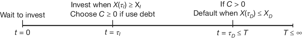
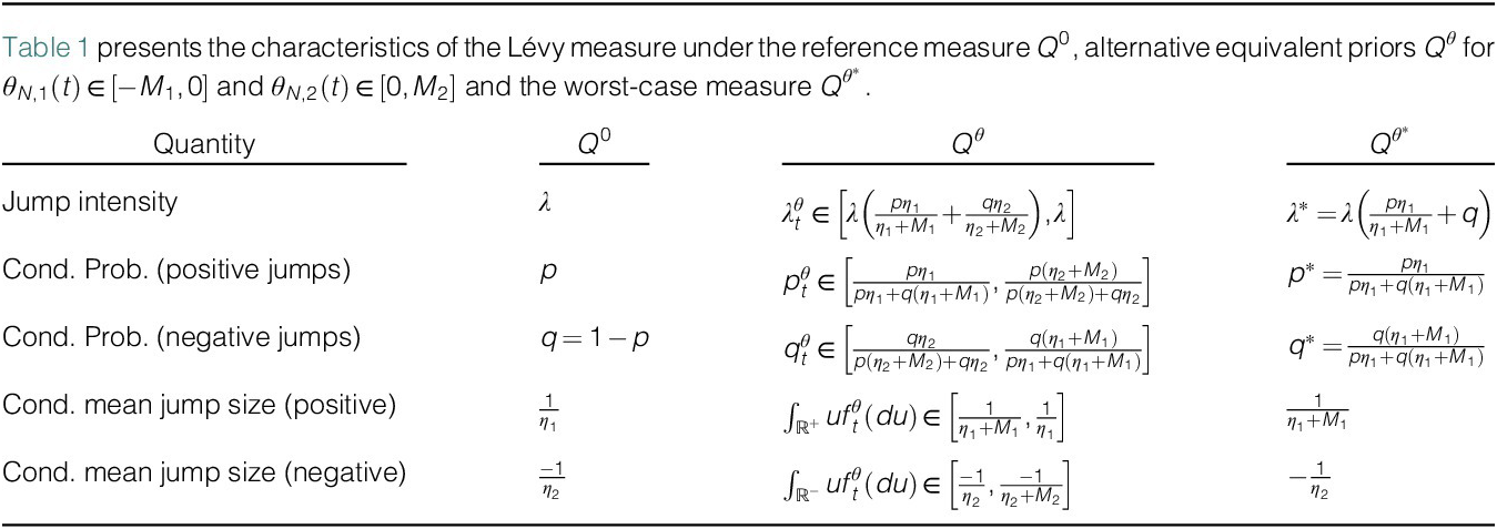
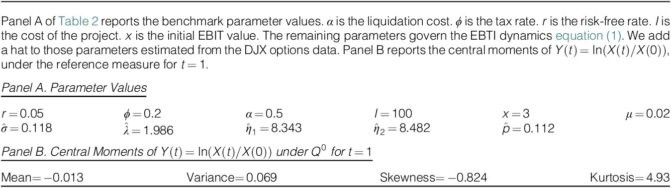
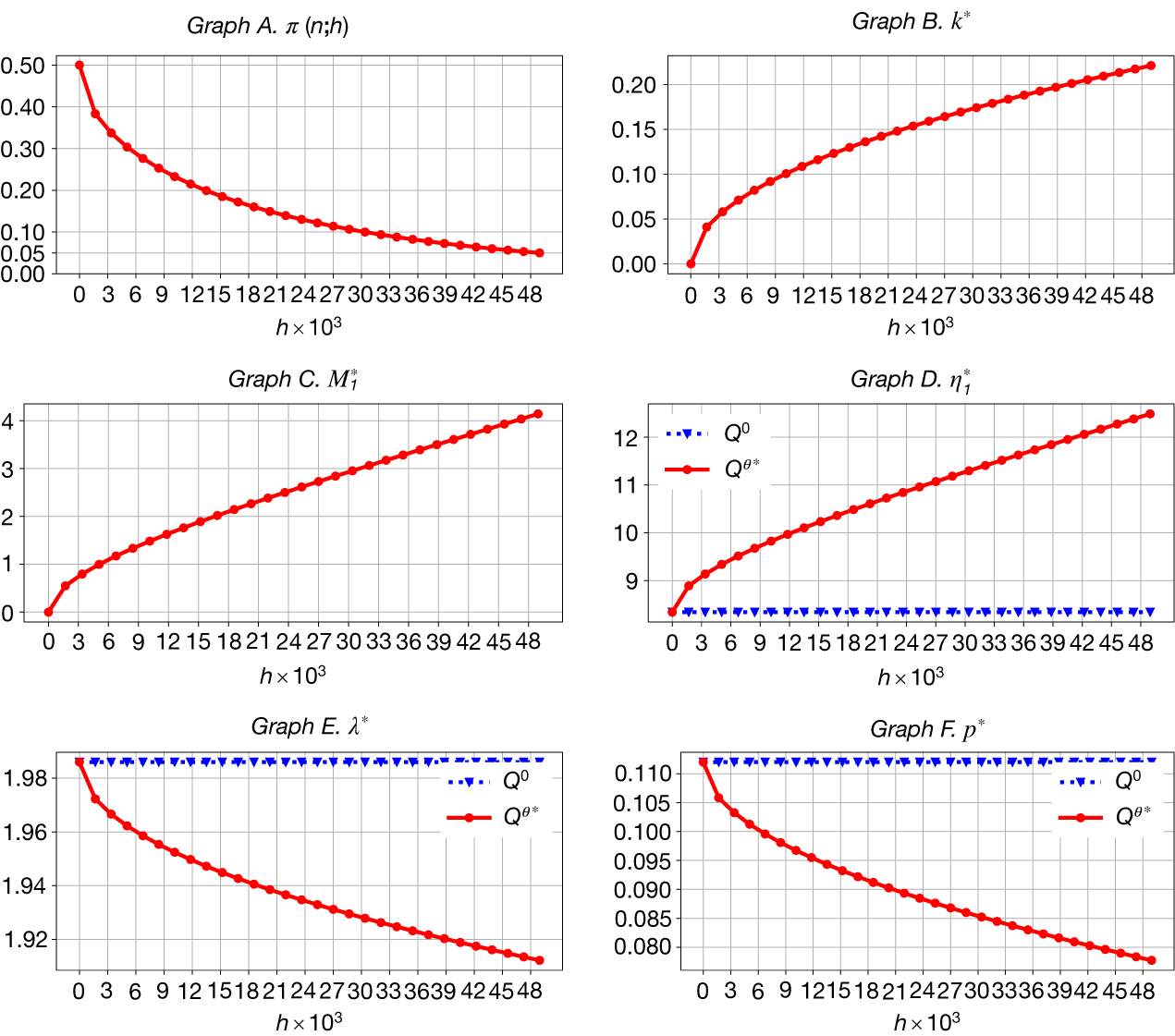


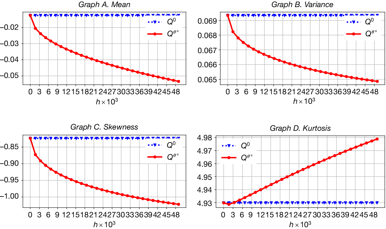


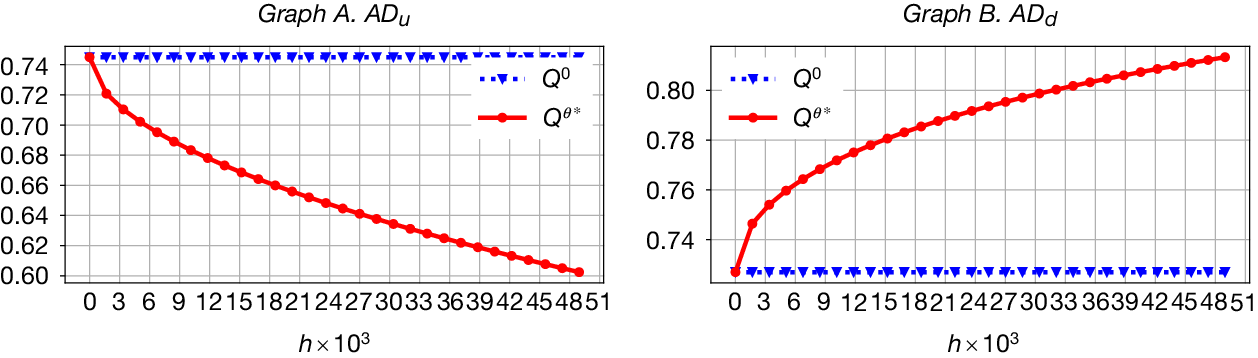


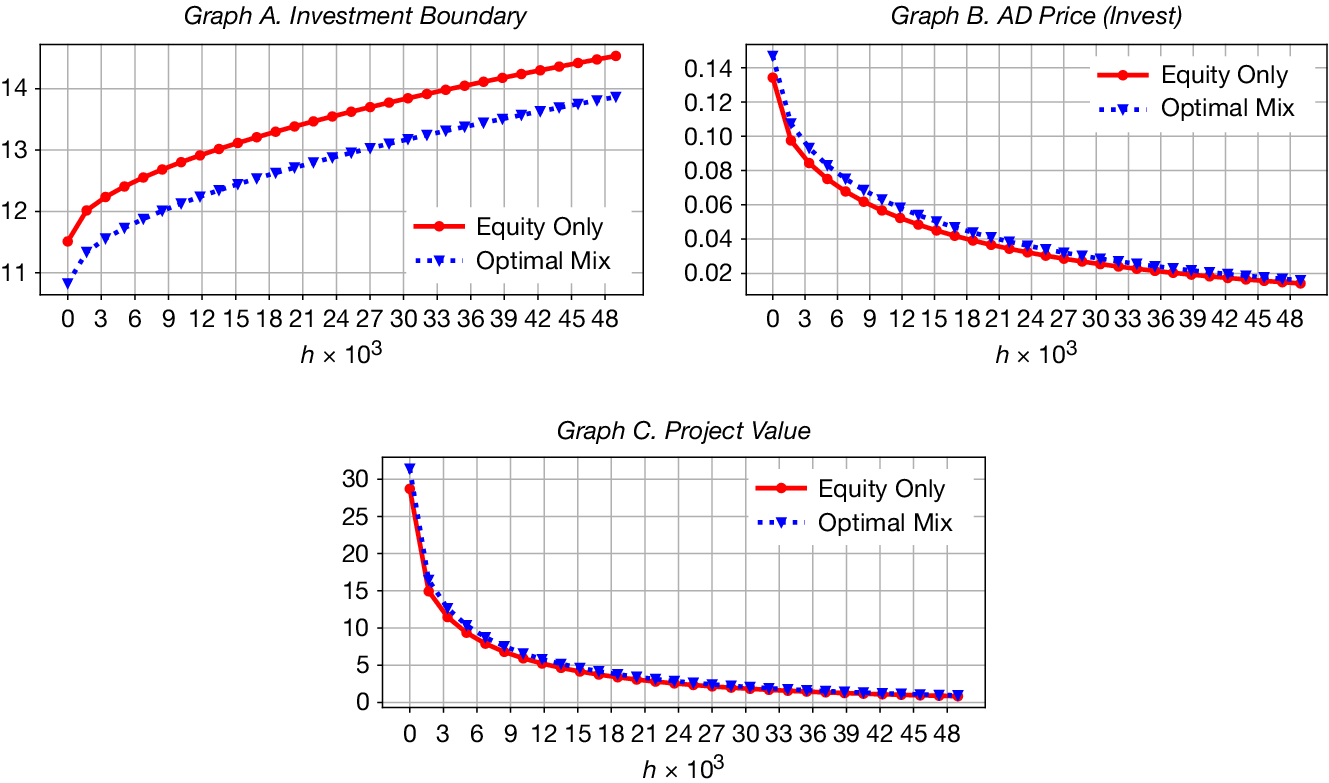


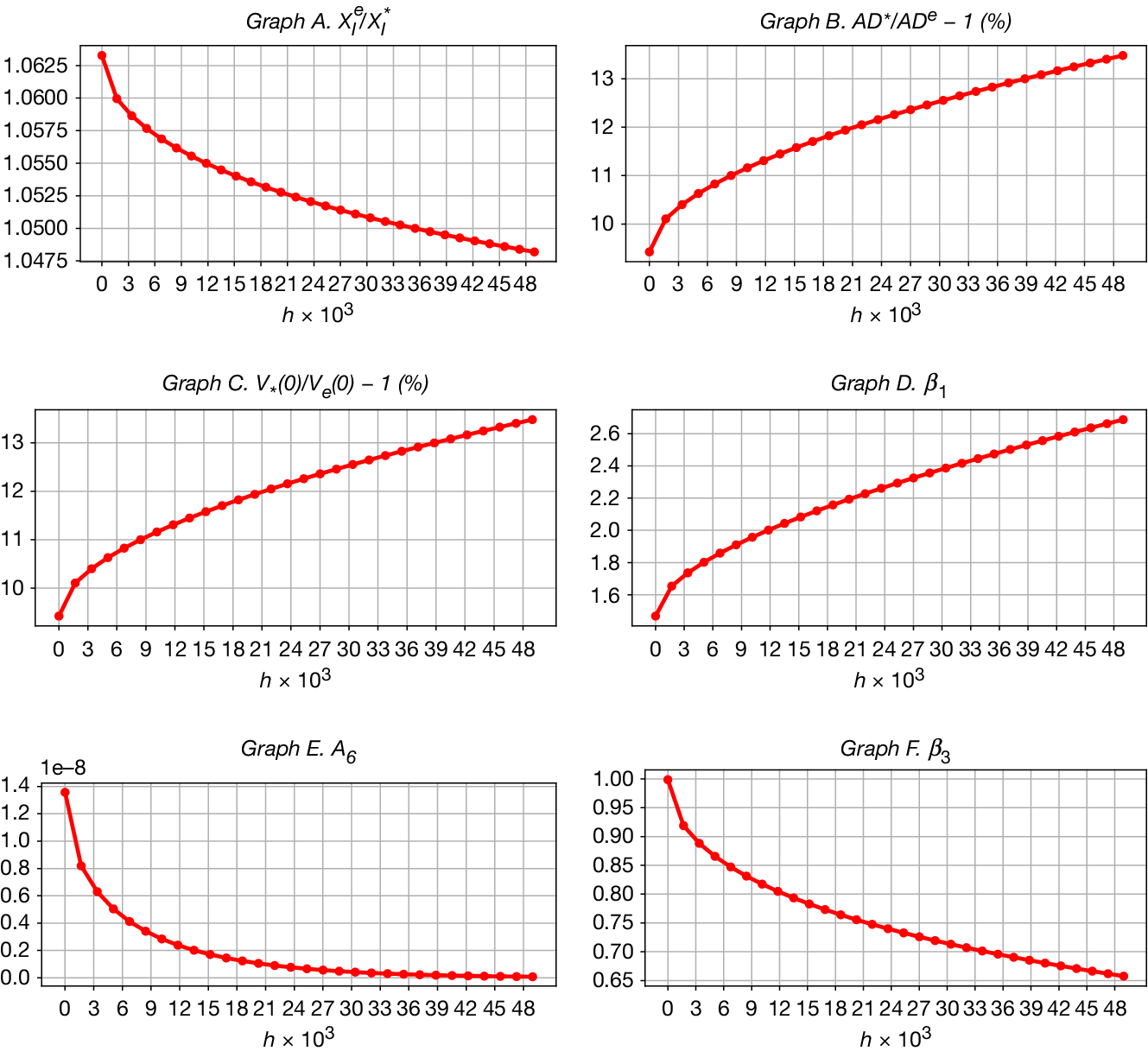


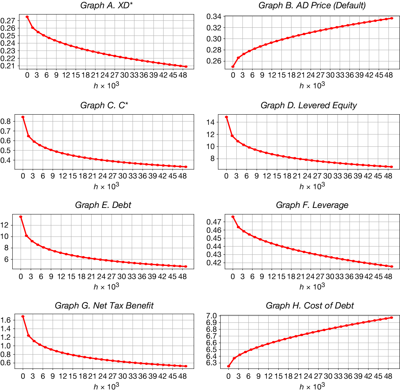


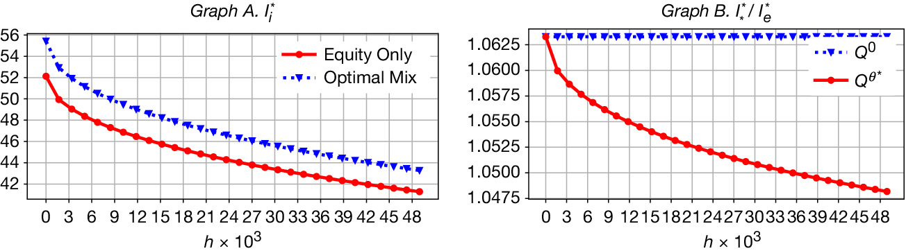


 Open access