


1. Introduction
Hoppers are extensively used in granular processing in diverse industries including pharmaceuticals, chemicals, food processing, fertiliser, bioenergy, cement, mining and agriculture (Miserque & Pirard Reference Miserque and Pirard2004; Anand et al. Reference Anand, Curtis, Wassgren, Hancock and Ketterhagen2008; Nourmohamadi-Moghadami et al. Reference Nourmohamadi-Moghadami, Zare, Stroshine and Kamfiroozi2020; Lu et al. Reference Lu, Jin, Klinger and Dai2021). For example, in the pharmaceutical industries, hoppers are used for dosing of active pharmaceutical ingredients and buffer materials in drug formulations, and in the chemical industries, they are used for storing raw materials, catalysts and products. Hoppers play an important role in granular processing, and improper functioning, for example, due to clogging, results is a lower usable capacity, which can adversely affect the manufacturing process. Clogging is due to arch formation, which results from the converging flow at the exit of the hopper and cohesive forces between particles. Cohesion also affects the flow pattern within hoppers. When cohesion between particles is low and the hopper angle is steep enough, all the particles move uniformly out of the system, and this flow pattern is called mass flow. Conversely, in cases with significant inter-particle cohesion, the funnel flow pattern is obtained, in which particles near the centre of the hopper exit first, followed by those closer to the hopper wall. Design of hoppers that deliver a reliable performance, thus, requires an understanding of the flow. The converging flow in hoppers, in the mass flow regime, has different rheological characteristics compared with shear flows (Bhateja & Khakhar Reference Bhateja and Khakhar2020; Momin & Khakhar Reference Momin and Khakhar2025). Consequently, characterising the flow in hoppers is also useful for the study of granular rheology in converging flows.
The focus of the present work is on the mass flow in hoppers in which clogging and cohesion are negligible, and we briefly review related previous studies. The mass flow rate ( $\dot {m}$
) in different hopper geometries has been shown to follow the Beverloo correlation (Beverloo, Leniger & Van de Velde Reference Beverloo, Leniger and Van de Velde1961), which for two-dimensional (2-D) systems is given by
$\dot {m}$
) in different hopper geometries has been shown to follow the Beverloo correlation (Beverloo, Leniger & Van de Velde Reference Beverloo, Leniger and Van de Velde1961), which for two-dimensional (2-D) systems is given by
 \begin{align} \dot {m} = C B\rho _p\phi _{b} \sqrt {g} \big(D_0 - kd_p \big)^{3/2} , \end{align}
where $g$
is the acceleration due to gravity,
$g$
is the acceleration due to gravity, $D_0$
and
$D_0$
and $B$
are the orifice width and thickness of the hopper,
$B$
are the orifice width and thickness of the hopper, $d_p$
and
$d_p$
and $\rho _p$
are the diameter and density of the particles and
$\rho _p$
are the diameter and density of the particles and $\phi _b$
is the bulk solid fraction of the particles. Also,
$\phi _b$
is the bulk solid fraction of the particles. Also, $C$
and
$C$
and $k$
are empirical parameters obtained by fitting to data.
$k$
are empirical parameters obtained by fitting to data.
Theoretical analyses of the velocity distribution in hoppers are relatively few. Savage (Reference Savage1965) showed that the velocity field in a conical hopper with frictionless walls is given by
 \begin{align} v_R =A/R^2, \qquad v_{\varTheta }=0. \end{align}
Here, $A$
is a constant, and
$A$
is a constant, and $R$
and
$R$
and $\varTheta$
are the radial distance and azimuthal angle relative to a spherical coordinate system with its origin at the apex of the cone. Similarly, for a wedge-shaped hopper with frictionless walls, the radial velocity, with respect to a cylindrical coordinate system with its origin at the apex of the wedge, is (Savage Reference Savage1965)
$\varTheta$
are the radial distance and azimuthal angle relative to a spherical coordinate system with its origin at the apex of the cone. Similarly, for a wedge-shaped hopper with frictionless walls, the radial velocity, with respect to a cylindrical coordinate system with its origin at the apex of the wedge, is (Savage Reference Savage1965)
 \begin{align} v_r =a/r, \qquad v_{\theta }=0, \end{align}
where $r$
is the radial distance,
$r$
is the radial distance, $\theta$
is the angle relative to the centreline of wedge and
$\theta$
is the angle relative to the centreline of wedge and $a$
is a constant. The Mohr–Coulomb yield condition was used as the constitutive model. Momin & Khakhar (Reference Momin and Khakhar2025) compared predictions of the Savage (Reference Savage1965) theory and predictions of a theory based on the
$a$
is a constant. The Mohr–Coulomb yield condition was used as the constitutive model. Momin & Khakhar (Reference Momin and Khakhar2025) compared predictions of the Savage (Reference Savage1965) theory and predictions of a theory based on the $\mu$
–
$\mu$
– $I$
model to discrete element method (DEM) simulations, where
$I$
model to discrete element method (DEM) simulations, where $\mu$
is the effective friction and
$\mu$
is the effective friction and $I$
is the inertial number. The theory based on the
$I$
is the inertial number. The theory based on the $\mu$
–
$\mu$
– $I$
model gave better predictions in a small region near the exit of the hopper, however, both theories gave nearly identical results in the rest of the hopper. Staron, Lagrée & Popinet (Reference Staron, Lagrée and Popinet2012) also showed that the
$I$
model gave better predictions in a small region near the exit of the hopper, however, both theories gave nearly identical results in the rest of the hopper. Staron, Lagrée & Popinet (Reference Staron, Lagrée and Popinet2012) also showed that the $\mu$
–
$\mu$
– $I$
model gives good predictions for draining of a rectangular hopper by comparison with results from contact dynamics simulations.
$I$
model gives good predictions for draining of a rectangular hopper by comparison with results from contact dynamics simulations.
Wall friction has a significant effect on the velocity field, and has been considered in a few papers (Jenike Reference Jenike1964; Savage Reference Savage1967; Brennen & Pearce Reference Brennen and Pearce1978; Kaza & Jackson Reference Kaza and Jackson1982; Prakash & Rao Reference Prakash and Rao1991; Gremaud et al. Reference Gremaud, Matthews and O’Malley2004, Reference Gremaud, Matthews and Schaeffer2006). Brennen & Pearce (Reference Brennen and Pearce1978) carried out a perturbation analysis for a purely frictional material considering the velocity field in a wedge-shaped hopper to be given by
 \begin{align} v_r = v_{r0}(r)+v_{r2}(r)(\theta /\theta _w)^2+\ldots , \\[-28pt] \nonumber \end{align}
 \begin{align} v_{\theta } = v_{\theta 1}(r)(\theta /\theta _w)+v_{\theta 3}(r)(\theta /\theta _w)^3+\ldots , \\[5pt] \nonumber \end{align}
where $\theta _w$
is the hopper half-angle. The Mohr–Coulomb condition was used as the constitutive model, along with the colinearity condition. To the first order of approximation, they found that
$\theta _w$
is the hopper half-angle. The Mohr–Coulomb condition was used as the constitutive model, along with the colinearity condition. To the first order of approximation, they found that $v_{r0}=-a/r$
,
$v_{r0}=-a/r$
, $v_{\theta 1}=0$
and
$v_{\theta 1}=0$
and $v_{r2}=-v_{r0}[2\mu _w\theta _w(1+\sin \beta )/\sin \beta ]$
, where
$v_{r2}=-v_{r0}[2\mu _w\theta _w(1+\sin \beta )/\sin \beta ]$
, where $a$
is a constant,
$a$
is a constant, $\mu _w$
is the wall friction coefficient and
$\mu _w$
is the wall friction coefficient and $\beta$
is the angle of internal friction of the particles. The solution is valid when
$\beta$
is the angle of internal friction of the particles. The solution is valid when $(\mu _w\theta _w/\sin \beta )$
is small. In the absence of wall friction (
$(\mu _w\theta _w/\sin \beta )$
is small. In the absence of wall friction ( $\mu _w=0$
), we have
$\mu _w=0$
), we have $v_{r2}=0$
and the solution reduces to the Savage (Reference Savage1965) result. The theories discussed above are purely frictional, and although they work well for steady flows, they are ill posed if used to simulate time-varying flows (Schaeffer Reference Schaeffer1987).
$v_{r2}=0$
and the solution reduces to the Savage (Reference Savage1965) result. The theories discussed above are purely frictional, and although they work well for steady flows, they are ill posed if used to simulate time-varying flows (Schaeffer Reference Schaeffer1987).
A number of experimental studies of the velocity field in hoppers have been reported. Nedderman (Reference Nedderman1988) described a method for determining the local velocity by placing a tracer particle at a precise radial and angular position ( $R, \varTheta$
) in a conical hopper and noting the time taken by the tracer particle to exit the hopper,
$R, \varTheta$
) in a conical hopper and noting the time taken by the tracer particle to exit the hopper, $T$
. As above,
$T$
. As above, $R$
and
$R$
and $\varTheta$
are relative to a spherical coordinate system with its origin at the apex of the cone. The experimental results showed, to a high degree of accuracy, that
$\varTheta$
are relative to a spherical coordinate system with its origin at the apex of the cone. The experimental results showed, to a high degree of accuracy, that
 \begin{align} R^3 - R_0^3 = 3f(\varTheta )T, \end{align}
where $R_0$
is the radius at the outlet of the hopper. The velocity field obtained was thus
$R_0$
is the radius at the outlet of the hopper. The velocity field obtained was thus
 \begin{align} v_R = f(\varTheta )/R^2; \qquad v_{\varTheta } = 0. \end{align}
Experiments with different mass flow rates and wall roughnesses showed that $f(\varTheta )$
depended on the wall roughness but was independent of the mass flow rate. Cleaver & Nedderman (Reference Cleaver and Nedderman1993) used a similar method and considered different materials. The results validated the conclusions of Nedderman (Reference Nedderman1988). Medina et al. (Reference Medina, Cordova, Luna and Trevino1998) used particle image velocimetry to measure particle velocities in a 2-D rectangular hopper, comprising a monolayer of particles. They found both the mean velocity profiles and fluctuation velocity profiles to be Gaussian. Choi, Kudrolli & Bazant (Reference Choi, Kudrolli and Bazant2005) used a similar technique for a quasi-2-D rectangular hopper of thickness 8.3 particle diameters and measured particle velocities at the front surface. They obtained Gaussian profiles at distances far from the outlet and compared their results with the kinematic model of Tüzün & Nedderman (Reference Tüzün and Nedderman1979). Gentzler & Tardos (Reference Gentzler and Tardos2009) used nuclear magnetic resonance imaging to obtain velocity and density distributions in two different geometries. They found a significant density variation in the flow. Finally, Vivanco, Rica & Melo (Reference Vivanco, Rica and Melo2012) used photoelastic disks, forming a monolayer, in a 2-D wedge-shaped hopper. They found significant arch formation, which affected the magnitude of the velocity fluctuations, but did not impact the average flow rate significantly. The radial velocity, with respect to a cylindrical coordinate system with its origin at the apex of the wedge, as above, was found to vary as
$f(\varTheta )$
depended on the wall roughness but was independent of the mass flow rate. Cleaver & Nedderman (Reference Cleaver and Nedderman1993) used a similar method and considered different materials. The results validated the conclusions of Nedderman (Reference Nedderman1988). Medina et al. (Reference Medina, Cordova, Luna and Trevino1998) used particle image velocimetry to measure particle velocities in a 2-D rectangular hopper, comprising a monolayer of particles. They found both the mean velocity profiles and fluctuation velocity profiles to be Gaussian. Choi, Kudrolli & Bazant (Reference Choi, Kudrolli and Bazant2005) used a similar technique for a quasi-2-D rectangular hopper of thickness 8.3 particle diameters and measured particle velocities at the front surface. They obtained Gaussian profiles at distances far from the outlet and compared their results with the kinematic model of Tüzün & Nedderman (Reference Tüzün and Nedderman1979). Gentzler & Tardos (Reference Gentzler and Tardos2009) used nuclear magnetic resonance imaging to obtain velocity and density distributions in two different geometries. They found a significant density variation in the flow. Finally, Vivanco, Rica & Melo (Reference Vivanco, Rica and Melo2012) used photoelastic disks, forming a monolayer, in a 2-D wedge-shaped hopper. They found significant arch formation, which affected the magnitude of the velocity fluctuations, but did not impact the average flow rate significantly. The radial velocity, with respect to a cylindrical coordinate system with its origin at the apex of the wedge, as above, was found to vary as
 \begin{align} v_r = [a\cos (\pi \theta /2\theta _w) + b]/r, \end{align}
where $a$
and
$a$
and $b$
are fitting constants, and
$b$
are fitting constants, and $\theta _w$
is the hopper half-angle. Several works are focused on a small region near the exit of 2-D hoppers (monolayer of particles) (Janda, Zuriguel & Maza Reference Janda, Zuriguel and Maza2012; Rubio-Largo et al. Reference Rubio-Largo, Janda, Maza, Zuriguel and Hidalgo2015; Gella, Maza & Zuriguel Reference Gella, Maza and Zuriguel2017), and have demonstrated excellent scaling of the velocity and solid fraction profiles for different orifice sizes. The velocity profiles are found to be parabolic in a Cartesian coordinate system,
$\theta _w$
is the hopper half-angle. Several works are focused on a small region near the exit of 2-D hoppers (monolayer of particles) (Janda, Zuriguel & Maza Reference Janda, Zuriguel and Maza2012; Rubio-Largo et al. Reference Rubio-Largo, Janda, Maza, Zuriguel and Hidalgo2015; Gella, Maza & Zuriguel Reference Gella, Maza and Zuriguel2017), and have demonstrated excellent scaling of the velocity and solid fraction profiles for different orifice sizes. The velocity profiles are found to be parabolic in a Cartesian coordinate system, $v_y\propto x^2$
, where the
$v_y\propto x^2$
, where the $y$
-axis is along the axis of the hopper. These results and the result of Vivanco et al. (Reference Vivanco, Rica and Melo2012) (1.8) are consistent with the theory of Brennen & Pearce (Reference Brennen and Pearce1978) (1.4), if we make the approximations
$y$
-axis is along the axis of the hopper. These results and the result of Vivanco et al. (Reference Vivanco, Rica and Melo2012) (1.8) are consistent with the theory of Brennen & Pearce (Reference Brennen and Pearce1978) (1.4), if we make the approximations $v_r\sim v_y$
,
$v_r\sim v_y$
, $x\sim r\theta$
and
$x\sim r\theta$
and $\cos (\pi \theta /2\theta _w)\approx 1- (\pi \theta /\theta _w)^2/8$
.
$\cos (\pi \theta /2\theta _w)\approx 1- (\pi \theta /\theta _w)^2/8$
.
In this work, we carry out an experimental study of the granular flow in a quasi-2-D wedge-shaped hopper with glass front and back walls. The study employs videography with image analysis and particle tracking to obtain the spatial variations of the velocity field and solid area fraction within the hopper. The objective of the study is to obtain the velocity field at a high spatial resolution for varying system parameters, which would be useful data for testing new theories. The parameters varied include the orifice size, roughness of the hopper sidewalls and particle size and density. Accurate empirical expressions for the velocity distribution in the system are also obtained from the measured velocities. The measured velocities are influenced by the friction of the front and back glass walls. To understand these effects we carry out DEM simulations for a system of the same size as the experimental hopper and calibrate the simulation parameters to match the experimental velocity profiles. Experimental details are given in the next section, followed by simulation details in § 3. Results and discussion are given in § 4 and conclusions in § 5.
2. Experimental details
Details of the experimental set-up and materials used are described first, followed by the procedure used for image analysis and the methods for data analysis.
(a) Schematic view of the wedge-shaped hopper used in the experiments. The screw is used to adjust the horizontal position of the left spacer and thus control the orifice width, $D_0$
. The handle is used to slide the stopper plate to block/unblock the orifice. The dimensions are in mm. (b) Photograph of the experimental set-up.
$D_0$
. The handle is used to slide the stopper plate to block/unblock the orifice. The dimensions are in mm. (b) Photograph of the experimental set-up.

2.1. Experimental system
Figure 1 shows the wedge-shaped hopper used in the experiments, which consists of two acrylic spacers between two glass plates with a cuboid feeder bin. The vertical glass plates of dimensions of $61 \ \mathrm{cm} \times 37 \ \mathrm{cm}$
, form the smooth front and rear-wall surfaces, and facilitate observation of the granular flow. The acrylic spacers, of thickness
$61 \ \mathrm{cm} \times 37 \ \mathrm{cm}$
, form the smooth front and rear-wall surfaces, and facilitate observation of the granular flow. The acrylic spacers, of thickness $B=1.2$
cm, are mirror symmetric with a hopper-section height of
$B=1.2$
cm, are mirror symmetric with a hopper-section height of $H=38.5$
cm and a wedge angle of 20 deg. to the vertical (figure 1
a). While one wedge-shaped spacer remains fixed, the other can slide, enabling the adjustment of the orifice size from 0 to 50 mm, by means of a screw. In each experiment, the hopper wall is set to a specific orifice size (
$H=38.5$
cm and a wedge angle of 20 deg. to the vertical (figure 1
a). While one wedge-shaped spacer remains fixed, the other can slide, enabling the adjustment of the orifice size from 0 to 50 mm, by means of a screw. In each experiment, the hopper wall is set to a specific orifice size ( $D_0$
) and the orifice is initially blocked using a sliding acrylic stopper plate, as shown in figure 1(a). The acrylic stopper is horizontally slid relative to the hopper outlet, enabling the flow of particles. Particles are continuously fed from the feeder bin placed at the top of the hopper and collected in a container located below the hopper. The design ensures a steady and continuous flow of particles over the duration of an experiment. The glass plates and spacers are fixed in a rigid steel frame to minimise vibrations caused by the flow of the material. A photograph of the set-up is shown in figure 1(b). Table 1 summarises the geometrical details of the experimental system. The roughness of the sidewalls is modified by pasting sandpaper of different grit sizes. Three specific grit sizes are used with grit numbers
$D_0$
) and the orifice is initially blocked using a sliding acrylic stopper plate, as shown in figure 1(a). The acrylic stopper is horizontally slid relative to the hopper outlet, enabling the flow of particles. Particles are continuously fed from the feeder bin placed at the top of the hopper and collected in a container located below the hopper. The design ensures a steady and continuous flow of particles over the duration of an experiment. The glass plates and spacers are fixed in a rigid steel frame to minimise vibrations caused by the flow of the material. A photograph of the set-up is shown in figure 1(b). Table 1 summarises the geometrical details of the experimental system. The roughness of the sidewalls is modified by pasting sandpaper of different grit sizes. Three specific grit sizes are used with grit numbers $Gn=100$
, 80 and 60, where the grit number (
$Gn=100$
, 80 and 60, where the grit number ( $Gn$
) represents the number of particles per square inch of sandpaper. A lower grit number indicates a rougher surface.
$Gn$
) represents the number of particles per square inch of sandpaper. A lower grit number indicates a rougher surface.
System parameters and measured diameters of the particles used. Here, SS denotes stainless steel particles and GS denotes glass particles; the appended number gives the nominal diameter. The mean values and the standard deviations of the particle diameters calculated from the measured particle size distributions are given.

Particle size distributions $P(d_p)$
, of (a) the stainless steel and (b) the glass particles. (c) Typical image of particles used to obtain the size distribution.
$P(d_p)$
, of (a) the stainless steel and (b) the glass particles. (c) Typical image of particles used to obtain the size distribution.

Stainless steel particles (denoted SS) with nominal diameters of 1 and 1.5 mm, and glass particles (denoted GS) with nominal diameters of 1, 1.5 and 3 mm are used. The glass particles are made of coloured glass, which helps in their detection during image analysis. The stainless steel particles are highly spherical. The size distributions of the particles are obtained by gluing the particles on a white paper, using a sieve to keep the particles apart (figure 2
c), and then using image analysis. The equivalent circular disk diameter is obtained from the measured projected area of each particle and around 2000 particles are measured for each case. The size distributions of the stainless steel and the glass particles are shown in figure 2, where $P(d_p)\Delta d_p$
is the number fraction of particles in the size range
$P(d_p)\Delta d_p$
is the number fraction of particles in the size range $(d_p,d_p+\Delta d_p)$
. The stainless steel particles have a narrower distribution than the glass particles, as can be inferred the higher peak values of the number fraction density (
$(d_p,d_p+\Delta d_p)$
. The stainless steel particles have a narrower distribution than the glass particles, as can be inferred the higher peak values of the number fraction density ( $P(d_p)$
). The mean diameters and the standard deviations, obtained from the size distributions, are given in table 1. The glass particles are slightly larger than the nominal values. The particle densities, determined using the liquid-displacement method, are 7.87 g cm
$P(d_p)$
). The mean diameters and the standard deviations, obtained from the size distributions, are given in table 1. The glass particles are slightly larger than the nominal values. The particle densities, determined using the liquid-displacement method, are 7.87 g cm $^{-3}$
and 2.47 g cm
$^{-3}$
and 2.47 g cm $^{-3}$
, for SS and GS, respectively. The method also yields the packed bed solid fraction for each of the particles, which are
$^{-3}$
, for SS and GS, respectively. The method also yields the packed bed solid fraction for each of the particles, which are $\phi _b=0.60$
for SS and
$\phi _b=0.60$
for SS and $\phi _b=0.62$
for GS.
$\phi _b=0.62$
for GS.
A high-speed camera (Photron FASTCAM SA3 model 120k-M3 with a Nikkor 24–85 mm f/2.8 Zoom lens) is used to record videos. The camera is adjusted so that the axis of the lens is perpendicular to the front glass plate of the hopper.
2.2. Experimental procedure
The stopper is closed and particles are filled into the hopper and the feeder bin. Two LED light sources are positioned in front of the wedge-shaped planar area of interest, to illuminate the front layer of particles, and the camera is focused to capture individual particles in the front layer. The camera is connected to a computer, which is used for controlling the camera and acquiring the images. Initially, both the camera and LED lights are turned on. Following that, the exit of the hopper is opened by sliding out the stopper, which allows granular particles to flow through the hopper. The flow is captured on video for 7–8 s, with a recording speed of 1000 frames per second (fps) at a resolution of $1024 \times 1024$
pixels, and an electronic shutter speed of 1/1000 s, corresponding to an exposure time of 1 ms. Each experiment is repeated five times, and the error bars shown in the results represent the standard error of the measurements.
$1024 \times 1024$
pixels, and an electronic shutter speed of 1/1000 s, corresponding to an exposure time of 1 ms. Each experiment is repeated five times, and the error bars shown in the results represent the standard error of the measurements.
Snapshots illustrating the procedure for image analysis and particle tracking for 1.5 mm glass particles (GS1.5). (a) image of particles in the hopper. (b) Image showing detected particles. (c), (d) Magnified view of a section of (a), (b) respectively. (e) Particle trajectories detected in a sequence of images. (f) Magnified view of a single trajectory.

2.3. Image analysis
Image analysis and particle tracking are done using FIJI/ImageJ (Schindelin et al. Reference Schindelin2012) and the MOSAIC plugin (Sbalzarini & Koumoutsakos Reference Sbalzarini and Koumoutsakos2005), respectively. The recorded videos are converted into a series of individual frames, which are imported into FIJI. A scale factor is set by measuring a known distance between two points of an attached scale. The scale factor is approximately 44 pixels cm−1 corresponding to a resolution of 0.22 mm. The imported images are first thresholded to highlight a bright spot on each particle (figure 3 a), and the circular boundary of each particle is obtained (figure 3 b), along with its centroid. Magnified views of a portion of the images are shown in figure 3(c,d). The process is repeated for each frame in the sequence to obtain the position coordinates of the particles. Particles in each pair of consecutive frames are linked to generate particle trajectories using the MOSAIC plugin, as shown in figure 3(e), with a magnified view of a single trajectory shown in figure 3(f).
(a) Schematic diagram of the wedge-shaped hopper along with the coordinate systems used in the analyses. (b) Snapshot of the DEM simulation domain showing the flowing particles.

Image analysis and particle tracking yield the sequence of positions of each particle, $i$
, in consecutive frames,
$i$
, in consecutive frames, $j$
, along a trajectory, (
$j$
, along a trajectory, ( $x_{\textit{ij}},y_{\textit{ij}}$
). The instantaneous velocities of particle,
$x_{\textit{ij}},y_{\textit{ij}}$
). The instantaneous velocities of particle, $i$
, in the
$i$
, in the $x$
- and
$x$
- and $y$
- directions are computed using the centred difference method as
$y$
- directions are computed using the centred difference method as
 \begin{align} c_{\textit{xi}}(x_{\textit{im}},y_{\textit{im}}) &= \frac {(x_{\textit{ij}} - x_{i(j - p)})}{({\rm d}t \times p)}, \\[-9pt] \nonumber\end{align}
 \begin{align} c_{\textit{yi}}(x_{\textit{im}},y_{\textit{im}}) &= \frac {(y_{\textit{ij}} - y_{i(j - p)})}{({\rm d}t \times p)}, \\[9pt] \nonumber\end{align}
where ${\rm d}t$
is the time between two frames,
${\rm d}t$
is the time between two frames, $x_{\textit{im}}=(x_{\textit{ij}} + x_{i(j - p)})/2$
and
$x_{\textit{im}}=(x_{\textit{ij}} + x_{i(j - p)})/2$
and $y_{\textit{im}}=(y_{\textit{ij}} + y_{i(j - p)})/2$
. We take
$y_{\textit{im}}=(y_{\textit{ij}} + y_{i(j - p)})/2$
. We take $p = 5$
to ensure a sufficiently large displacement of particles for the calculation of the instantaneous velocities, corresponding to a frame rate of 200 fps. Using
$p = 5$
to ensure a sufficiently large displacement of particles for the calculation of the instantaneous velocities, corresponding to a frame rate of 200 fps. Using $p=3$
and
$p=3$
and $p=8$
in the analysis gave nearly identical results. The region is divided into square bins of size
$p=8$
in the analysis gave nearly identical results. The region is divided into square bins of size ${\rm d}x \times {\rm d}y = 0.2 \ \mathrm{cm} \times 0.2 \ \mathrm{cm}$
. The average velocity in a bin is determined using the equations
${\rm d}x \times {\rm d}y = 0.2 \ \mathrm{cm} \times 0.2 \ \mathrm{cm}$
. The average velocity in a bin is determined using the equations
 \begin{align} v_x(x, y) = \frac {1}{N}\sum _{i=1}^N c_{\textit{xi}},\qquad v_y(x, y) = \frac {1}{N}\sum _{i=1}^N c_{\textit{yi}}, \end{align}
where $N$
is the number of particles in the bin, with its centre at
$N$
is the number of particles in the bin, with its centre at $(x,y)$
. The area fraction of particles in a bin is calculated as
$(x,y)$
. The area fraction of particles in a bin is calculated as
 \begin{align} \phi = \pi d_p^2N/(4 {\rm d}x^2). \end{align}
In cylindrical coordinates, defined in figure 4(a), the wedge-shaped region is divided into bins of dimensions $r{\rm d}\theta \times {\rm d}r$
with
$r{\rm d}\theta \times {\rm d}r$
with ${\rm d}r = 0.2 \ \mathrm{cm}$
and
${\rm d}r = 0.2 \ \mathrm{cm}$
and ${\rm d}\theta = 2 ^{\circ }$
. The radial and tangential components of the velocity are obtained as
${\rm d}\theta = 2 ^{\circ }$
. The radial and tangential components of the velocity are obtained as
 \begin{align} c_{\textit{ri}} &= {c_{\textit{xi}} x_{\textit{im}}}/{r_i} + {c_{\textit{yi}} y_{\textit{im}}}/{r_i}, \\[-9pt] \nonumber\end{align}
 \begin{align} c_{\theta i} &= {c_{\textit{xi}} y_{\textit{im}}}/{r_i} - {c_{\textit{yi}} x_{\textit{im}}}/{r_i}, \\[9pt] \nonumber\end{align}
where $r_i = (x_{\textit{im}}^2+y_{\textit{im}}^2)^{1/2}$
and
$r_i = (x_{\textit{im}}^2+y_{\textit{im}}^2)^{1/2}$
and $\theta _i=\tan ^{-1}(|x_{\textit{im}}/y_{\textit{im}}|)$
. The average radial and tangential components of the velocity are
$\theta _i=\tan ^{-1}(|x_{\textit{im}}/y_{\textit{im}}|)$
. The average radial and tangential components of the velocity are
 \begin{eqnarray} v_r (r, \theta ) = \frac {1}{N}\sum _{i=1}^N c_{\textit{ri}},\qquad v_{\theta }(r, \theta ) = \frac {1}{N}\sum _{i=1}^N c_{\theta i}, \end{eqnarray}
and the particle area fraction in the bin in this case is
 \begin{align} \phi (r, \theta ) = \pi d_p^2 N/(4r{\rm d}{\theta }{\rm d}r), \end{align}
where $(r,\theta )$
are the coordinates of the centre of the bin. Again, we report absolute values of the velocities,
$(r,\theta )$
are the coordinates of the centre of the bin. Again, we report absolute values of the velocities, $v_r$
and
$v_r$
and $v_{\theta }$
. We also calculated the root-mean-square (r.m.s.) fluctuation velocities as
$v_{\theta }$
. We also calculated the root-mean-square (r.m.s.) fluctuation velocities as
 \begin{eqnarray} u_r = \sqrt {\left (\frac {1}{N}\sum _{i=1}^N c_{\textit{ri}}^2\right ) - v_r^2},\qquad u_{\theta } = \sqrt {\left (\frac {1}{N}\sum _{i=1}^N c_{\theta i}^2\right ) - v_{\theta }^2}. \end{eqnarray}
Variation of the radial velocity, $v_r$
with time,
$v_r$
with time, $t$
, at
$t$
, at $r=8.75$
cm and
$r=8.75$
cm and $\theta =1$
deg., for SS1.5 particles with an orifice size,
$\theta =1$
deg., for SS1.5 particles with an orifice size, $D_0 = 2.5$
cm.
$D_0 = 2.5$
cm.

2.4. Experimental velocity transient
The transient variation of the experimental radial velocity $v_r(r, \theta ,t)$
was studied to characterise the approach of the flow to a steady state. Figure 5 shows the variation of the radial velocity (
$v_r(r, \theta ,t)$
was studied to characterise the approach of the flow to a steady state. Figure 5 shows the variation of the radial velocity ( $v_r$
) at position
$v_r$
) at position $r=8.75$
cm and
$r=8.75$
cm and $\theta =1$
deg. with time for 1.5 mm stainless steel particles (SS1.5) and an orifice size
$\theta =1$
deg. with time for 1.5 mm stainless steel particles (SS1.5) and an orifice size $D_0 = 2.5$
cm. The velocity rapidly increases to a peak in 0.5 s and then reduces slightly. A steady velocity of approximately 27.5 cm s−1 is obtained after approximately 1 s. The time taken to slide out the acrylic block also contributes to the transient. These results suggest that a time duration of 2 s is sufficient to achieve a steady-state flow for all systems considered in this study. The data reported below are all for times beyond 2 s.
$D_0 = 2.5$
cm. The velocity rapidly increases to a peak in 0.5 s and then reduces slightly. A steady velocity of approximately 27.5 cm s−1 is obtained after approximately 1 s. The time taken to slide out the acrylic block also contributes to the transient. These results suggest that a time duration of 2 s is sufficient to achieve a steady-state flow for all systems considered in this study. The data reported below are all for times beyond 2 s.
3. Simulation details
The DEM simulations are carried out in a system of the same dimensions as the experimental set-up for $D_0 = 2.5$
cm and for glass beads of nominal diameter
$D_0 = 2.5$
cm and for glass beads of nominal diameter $d_p = 1.5$
mm (GS1.5), using the open source software, LAMMPS (Plimpton Reference Plimpton1995). A snapshot of the system geometry used is shown in figure 4(b). The height of the hopper is
$d_p = 1.5$
mm (GS1.5), using the open source software, LAMMPS (Plimpton Reference Plimpton1995). A snapshot of the system geometry used is shown in figure 4(b). The height of the hopper is $H = 38.5$
cm and the wedge half-angle is
$H = 38.5$
cm and the wedge half-angle is $20^{\circ }$
. The thickness of hopper in the
$20^{\circ }$
. The thickness of hopper in the $z$
-direction is
$z$
-direction is $B = 1.2$
cm. A total of 120 000 particles of the measured diameters and with a size polydispersity equal to the standard deviation (
$B = 1.2$
cm. A total of 120 000 particles of the measured diameters and with a size polydispersity equal to the standard deviation ( $d_p=1.86\pm 0.17$
, table 1) are used. Periodic boundary conditions are applied in the
$d_p=1.86\pm 0.17$
, table 1) are used. Periodic boundary conditions are applied in the $y$
-direction so that particles leaving the hopper are fed back at the top. The sidewalls are frictional with a coefficient of friction,
$y$
-direction so that particles leaving the hopper are fed back at the top. The sidewalls are frictional with a coefficient of friction, $\mu _w$
. The front and back walls are also frictional with a coefficient of friction,
$\mu _w$
. The front and back walls are also frictional with a coefficient of friction, $\mu _g$
.
$\mu _g$
.
The Hookean model is used to compute the force ( $\boldsymbol{F}_{\textit{ij}}$
) between a pair of particles in contact,
$\boldsymbol{F}_{\textit{ij}}$
) between a pair of particles in contact, $i$
and
$i$
and $j$
, as
$j$
, as
 \begin{align} \boldsymbol{F}_{\textit{ij}} = \left ( k_n \delta \boldsymbol{n}_{\textit{ij}} - m_{\textit{eff}} \gamma _n \boldsymbol{v}_n \right ) - k_t \Delta \boldsymbol{s}_{\textit{ij}}, \end{align}
where $k_n$
and
$k_n$
and $k_t$
are elastic constants for normal and tangential deformation, respectively, and
$k_t$
are elastic constants for normal and tangential deformation, respectively, and $\gamma _n$
is the viscoelastic constant for normal damping. Also,
$\gamma _n$
is the viscoelastic constant for normal damping. Also, $\delta = ( (d_i + d_j)/2 - |\boldsymbol{x}_i - \boldsymbol{x}_j| )$
is the overlap between particles,
$\delta = ( (d_i + d_j)/2 - |\boldsymbol{x}_i - \boldsymbol{x}_j| )$
is the overlap between particles, $\boldsymbol{n}_{\textit{ij}}$
is the unit vector along the line joining the centres of the two particles,
$\boldsymbol{n}_{\textit{ij}}$
is the unit vector along the line joining the centres of the two particles, $m_{\textit{eff}} = m_im_j/(m_i+m_j)$
and
$m_{\textit{eff}} = m_im_j/(m_i+m_j)$
and $\Delta \boldsymbol{s}_{\textit{ij}}$
is the tangential displacement vector between the two particles and is normalised to ensure
$\Delta \boldsymbol{s}_{\textit{ij}}$
is the tangential displacement vector between the two particles and is normalised to ensure $k_t |\Delta \boldsymbol{s}_{\textit{ij}}|/k_n\delta \leqslant \mu _p$
, where
$k_t |\Delta \boldsymbol{s}_{\textit{ij}}|/k_n\delta \leqslant \mu _p$
, where $ \mu _p$
is the inter-particle friction.
$ \mu _p$
is the inter-particle friction.
The parameters used in the simulations are given in table 2 and the coefficient of restitution for the parameters used is $e = 0.9$
. The time step used in the simulations is
$e = 0.9$
. The time step used in the simulations is $1.2 \times 10^{-6}$
s, which corresponds to 2 % of the time for a binary collision (Silbert et al. Reference Silbert, Ertaş, Grest, Halsey, Levine and Plimpton2001). Averaging is done over 500,000 time steps after a steady state is reached. The three friction coefficients:
$1.2 \times 10^{-6}$
s, which corresponds to 2 % of the time for a binary collision (Silbert et al. Reference Silbert, Ertaş, Grest, Halsey, Levine and Plimpton2001). Averaging is done over 500,000 time steps after a steady state is reached. The three friction coefficients: $\mu _g, \mu _p, \mu _w$
are varied over the values given in table 2, keeping the other parameters fixed. The mass flow rate,
$\mu _g, \mu _p, \mu _w$
are varied over the values given in table 2, keeping the other parameters fixed. The mass flow rate, $\dot {m}$
, is computed by averaging the mass flux at the exit of the hopper, and the velocity distribution,
$\dot {m}$
, is computed by averaging the mass flux at the exit of the hopper, and the velocity distribution, $v_r(r,\theta )$
, is obtained as discussed in the previous section, considering only particles in layers of thickness
$v_r(r,\theta )$
, is obtained as discussed in the previous section, considering only particles in layers of thickness $d_p$
adjacent to the front and back walls.
$d_p$
adjacent to the front and back walls.
Parameter values used in the DEM simulations.

4. Results and discussion
We first present experimental results for the spatial distributions of the velocities and solid area fractions in the hopper (§ 4.1), followed by a discussion of the typical experimental velocity profiles obtained (§ 4.2). Results of the parametric study, varying the particle type, orifice width and sidewall roughness in the experiments, are given in § 4.3. Variation of the measured mass flow rates are presented next (§ 4.4), followed by the simulation results (§ 4.5).
Spatial distribution of the magnitude of the vertical velocity ( $|v_y|$
) in the hopper for six different orifice sizes (
$|v_y|$
) in the hopper for six different orifice sizes ( $D_0$
) for GS1.5 particles. Panels show (a)
$D_0$
) for GS1.5 particles. Panels show (a) $D_0=1.0$
, (b)
$D_0=1.0$
, (b) $D_0=1.5$
, (c)
$D_0=1.5$
, (c) $D_0=2.0$
, (d)
$D_0=2.0$
, (d) $D_0=2.5$
, (e)
$D_0=2.5$
, (e) $D_0=3.0$
and (f)
$D_0=3.0$
and (f) $D_0=3.5$
cm.
$D_0=3.5$
cm.

4.1. Spatial distributions
Figure 6 shows a colour map of the distribution of the magnitude of the vertical velocity, $v_y$
, for six different orifice sizes (
$v_y$
, for six different orifice sizes ( $D_0 = 1.0$
, 1.5, 2.0, 2.5, 3.0 and 3.5 cm) using square bins of side
$D_0 = 1.0$
, 1.5, 2.0, 2.5, 3.0 and 3.5 cm) using square bins of side ${\rm d}x = 2$
mm. The velocity distributions are symmetric about the centreline axis, as expected. Figure 6 indicates that increasing the orifice size increases the velocity magnitude and, for a given orifice size, the velocity is highest close to the outlet and the centreline, decreasing towards the sidewalls and the top of the hopper. The results are similar to previous experimental results (Mort et al. Reference Mort, Michaels, Behringer, Campbell, Kondic, Langroudi, Shattuck, Tang, Tardos and Wassgren2015). Figure 7 shows the horizontal velocity (
${\rm d}x = 2$
mm. The velocity distributions are symmetric about the centreline axis, as expected. Figure 6 indicates that increasing the orifice size increases the velocity magnitude and, for a given orifice size, the velocity is highest close to the outlet and the centreline, decreasing towards the sidewalls and the top of the hopper. The results are similar to previous experimental results (Mort et al. Reference Mort, Michaels, Behringer, Campbell, Kondic, Langroudi, Shattuck, Tang, Tardos and Wassgren2015). Figure 7 shows the horizontal velocity ( $v_x$
) distributions for the different orifice sizes. The magnitude of the velocities is approximately 50 times lower than the vertical velocity,
$v_x$
) distributions for the different orifice sizes. The magnitude of the velocities is approximately 50 times lower than the vertical velocity, $v_y$
. The distributions are symmetric about the centreline and the velocities are highest near the exit and zero at the centreline and the sidewalls. The corresponding distribution of particle area fraction (
$v_y$
. The distributions are symmetric about the centreline and the velocities are highest near the exit and zero at the centreline and the sidewalls. The corresponding distribution of particle area fraction ( $\phi$
) in the hopper is shown in figure 8. The area fraction remains approximately constant at
$\phi$
) in the hopper is shown in figure 8. The area fraction remains approximately constant at $\phi =0.70$
throughout the hopper, except for lower values near the outlet for the larger orifice sizes, due to the higher flow rates. The measured area fractions are a rough measure of the bulk solid fraction, since only the particles in a layer adjacent to the front glass plate are counted.
$\phi =0.70$
throughout the hopper, except for lower values near the outlet for the larger orifice sizes, due to the higher flow rates. The measured area fractions are a rough measure of the bulk solid fraction, since only the particles in a layer adjacent to the front glass plate are counted.
Horizontal velocity ( $v_x$
) distribution in the hopper for six different orifice sizes (
$v_x$
) distribution in the hopper for six different orifice sizes ( $D_0$
) for GS1.5 particles. Panels show (a)
$D_0$
) for GS1.5 particles. Panels show (a) $D_0=1.0$
, (b)
$D_0=1.0$
, (b) $D_0=1.5$
, (c)
$D_0=1.5$
, (c) $D_0=2.0$
, (d)
$D_0=2.0$
, (d) $D_0=2.5$
, (e)
$D_0=2.5$
, (e) $D_0=3.0$
and (f)
$D_0=3.0$
and (f) $D_0=3.5$
cm.
$D_0=3.5$
cm.

Solid area fraction ( $\phi$
) distribution in the hopper for six different orifice sizes (
$\phi$
) distribution in the hopper for six different orifice sizes ( $D_0$
) for GS1.5 particles. Panels show (a)
$D_0$
) for GS1.5 particles. Panels show (a) $D_0=1.0$
, (b)
$D_0=1.0$
, (b) $D_0=1.5$
, (c)
$D_0=1.5$
, (c) $D_0=2.0$
, (d)
$D_0=2.0$
, (d) $D_0=2.5$
, (e)
$D_0=2.5$
, (e) $D_0=3.0$
and (f)
$D_0=3.0$
and (f) $D_0=3.5$
cm.
$D_0=3.5$
cm.

Variation of the measured radial velocity ( $v_r$
) with the square of the scaled angle (
$v_r$
) with the square of the scaled angle ( $(\theta /\theta _w)^2$
) for GS1.5 particles with orifice size
$(\theta /\theta _w)^2$
) for GS1.5 particles with orifice size $D_0 = 2.5$
cm at different radial positions,
$D_0 = 2.5$
cm at different radial positions, $r$
(symbols). Error bars indicate the standard error. Lines are fits of (4.1) to the data. (b) Variation of the fitted centreline velocity (
$r$
(symbols). Error bars indicate the standard error. Lines are fits of (4.1) to the data. (b) Variation of the fitted centreline velocity ( $v_{r0})$
) with
$v_{r0})$
) with $1/r$
, and (c) fitted values of the effective wall friction (
$1/r$
, and (c) fitted values of the effective wall friction ( $F$
) with radius (
$F$
) with radius ( $r$
). The lines in (b) and (c) are fits of (4.2) and (4.3) to the simulation data.
$r$
). The lines in (b) and (c) are fits of (4.2) and (4.3) to the simulation data.

4.2. Velocity profiles
Figure 9(a) shows the variation of the measured radial velocity ( $v_r$
, symbols) with the square of the scaled angle (
$v_r$
, symbols) with the square of the scaled angle ( $(\theta /\theta _w)^2$
) at different radial positions (
$(\theta /\theta _w)^2$
) at different radial positions ( $r$
) for an orifice size of
$r$
) for an orifice size of $D_0=2.5$
cm and glass particles of size
$D_0=2.5$
cm and glass particles of size $d_p = 1.5$
mm (GS1.5), following Brennen & Pearce (Reference Brennen and Pearce1978) (1.4). The error bars are small (standard error less than 2 %), indicating the accuracy of the measurements. In all cases, the variation is linear, as predicted by the theory of Brennen & Pearce (Reference Brennen and Pearce1978) (1.4), except for the last point (
$d_p = 1.5$
mm (GS1.5), following Brennen & Pearce (Reference Brennen and Pearce1978) (1.4). The error bars are small (standard error less than 2 %), indicating the accuracy of the measurements. In all cases, the variation is linear, as predicted by the theory of Brennen & Pearce (Reference Brennen and Pearce1978) (1.4), except for the last point ( $\theta \approx \theta _w$
), which deviates slightly from linearity due to wall effects. However, the condition for validity of the theory (
$\theta \approx \theta _w$
), which deviates slightly from linearity due to wall effects. However, the condition for validity of the theory ( $\mu _w\theta _w/\sin \beta \ll 1$
) is not satisfied, based on estimates obtained from DEM calibration results discussed in § 4.5. The calibration yields
$\mu _w\theta _w/\sin \beta \ll 1$
) is not satisfied, based on estimates obtained from DEM calibration results discussed in § 4.5. The calibration yields $\mu _w=0.4$
and
$\mu _w=0.4$
and $\beta =21.8$
deg. so that
$\beta =21.8$
deg. so that $\mu _w\theta _w/\sin \beta =0.376$
. We thus consider a radial velocity equation of the same form as (1.4), and given by
$\mu _w\theta _w/\sin \beta =0.376$
. We thus consider a radial velocity equation of the same form as (1.4), and given by
 \begin{align} v_r(r,\theta ) = v_{r0}(r)\big [1-F(r)(\theta /\theta _w)^2\big ], \end{align}
where $v_{r0}(r)$
is the centreline velocity and
$v_{r0}(r)$
is the centreline velocity and $F(r)$
is related to the wall friction, but do not constrain
$F(r)$
is related to the wall friction, but do not constrain $F$
to be small or of the form given by the Brennen & Pearce (Reference Brennen and Pearce1978) theory. In physical terms, the factor
$F$
to be small or of the form given by the Brennen & Pearce (Reference Brennen and Pearce1978) theory. In physical terms, the factor $(1{-}F)$
represents the ratio of the radial velocity at the wall (slip velocity,
$(1{-}F)$
represents the ratio of the radial velocity at the wall (slip velocity, $v_r(r,\theta _w)$
) to the radial velocity at the centreline (
$v_r(r,\theta _w)$
) to the radial velocity at the centreline ( $v_{r0}(r)$
), and thus we refer to
$v_{r0}(r)$
), and thus we refer to $F$
as the effective wall friction. For smooth walls, the effective wall friction,
$F$
as the effective wall friction. For smooth walls, the effective wall friction, $F$
, is in the range (0,1), where
$F$
, is in the range (0,1), where $F=1$
corresponds to the no-slip condition at the wall (
$F=1$
corresponds to the no-slip condition at the wall ( $v_r(r,\theta _w)=0$
), and
$v_r(r,\theta _w)=0$
), and $F=0$
to perfect slip at the wall (
$F=0$
to perfect slip at the wall ( $v_r(r,\theta _w)=v_{r0}(r)$
). For rough walls, values of the effective wall friction larger than unity are obtained (
$v_r(r,\theta _w)=v_{r0}(r)$
). For rough walls, values of the effective wall friction larger than unity are obtained ( $F\gt 1$
). This corresponds to the radial velocity,
$F\gt 1$
). This corresponds to the radial velocity, $v_r$
, becoming zero at angles
$v_r$
, becoming zero at angles $\theta \lt \theta _w$
, resulting in a near stagnant zone near the walls, as shown below.
$\theta \lt \theta _w$
, resulting in a near stagnant zone near the walls, as shown below.
The lines in figure 9(a) are fits of (4.1) to the data, and show an excellent match for all the radial distances (coefficient of determination, $R^2\gt 0.99$
). The fitted values of
$R^2\gt 0.99$
). The fitted values of $v_{r0}$
and
$v_{r0}$
and $F$
at each value of the radial distance,
$F$
at each value of the radial distance, $r$
, are shown as symbols in figures 9(b) and 9(c), respectively. The centreline velocity,
$r$
, are shown as symbols in figures 9(b) and 9(c), respectively. The centreline velocity, $v_{r0}$
, varies linearly with the inverse of the radial distance (figure 9
b), and the line in the figure is a fit of
$v_{r0}$
, varies linearly with the inverse of the radial distance (figure 9
b), and the line in the figure is a fit of
 \begin{align} v_{r0}(r) = a_0/r + a_1, \end{align}
to the data. The fit is very good ( $R^2\gt 0.99$
), and yields
$R^2\gt 0.99$
), and yields $a_0 = 214$
,
$a_0 = 214$
, $a_1 = 2.4$
. Thus, the centreline velocity deviates slightly from the Savage (Reference Savage1965) result (1.3), in which
$a_1 = 2.4$
. Thus, the centreline velocity deviates slightly from the Savage (Reference Savage1965) result (1.3), in which $a_1=0$
. Figure 9(c) indicates that the factor
$a_1=0$
. Figure 9(c) indicates that the factor $F$
(symbols) increases linearly with radial distance,
$F$
(symbols) increases linearly with radial distance, $r$
, to a reasonable approximation. The data indicate that the slip velocity ratio,
$r$
, to a reasonable approximation. The data indicate that the slip velocity ratio, $v_r(r,\theta _w)/v_{r0}(r)=(1{-}F)$
, reduces with radial distance, from
$v_r(r,\theta _w)/v_{r0}(r)=(1{-}F)$
, reduces with radial distance, from $(1{-}F)=0.7$
near the outlet to
$(1{-}F)=0.7$
near the outlet to $(1-F)=0.2$
near the middle of the hopper. Thus, the effective wall friction,
$(1-F)=0.2$
near the middle of the hopper. Thus, the effective wall friction, $F$
, increases with increasing radial distance. The line in figure 9(c) is a linear fit of
$F$
, increases with increasing radial distance. The line in figure 9(c) is a linear fit of
 \begin{align} F(r) = b_0 + b_1r \end{align}
to the data, and yields $b_0 = 0.23$
, and
$b_0 = 0.23$
, and $b_1 = 0.03$
with a coefficient of determination,
$b_1 = 0.03$
with a coefficient of determination, $R^2\gt 0.96$
. The results presented above indicate that the scaling with respect to
$R^2\gt 0.96$
. The results presented above indicate that the scaling with respect to $\theta /\theta _w$
from the Brennen & Pearce (Reference Brennen and Pearce1978) theory is valid even when
$\theta /\theta _w$
from the Brennen & Pearce (Reference Brennen and Pearce1978) theory is valid even when $F$
is not small, as required by the theory. The above results are in contrast to previous results (Nedderman Reference Nedderman1988; Cleaver & Nedderman Reference Cleaver and Nedderman1993; Vivanco et al. Reference Vivanco, Rica and Melo2012), which reported the velocity field to be purely radial, with a zero tangential velocity (
$F$
is not small, as required by the theory. The above results are in contrast to previous results (Nedderman Reference Nedderman1988; Cleaver & Nedderman Reference Cleaver and Nedderman1993; Vivanco et al. Reference Vivanco, Rica and Melo2012), which reported the velocity field to be purely radial, with a zero tangential velocity ( $v_\theta =0$
), corresponding to
$v_\theta =0$
), corresponding to $a_1=b_1=0$
.
$a_1=b_1=0$
.
The small deviation of $F(r)$
from linearity in figure 9(c) is a consequence of the magnification of errors, since a small error in the velocity makes a large change in the slope, which is used to calculate
$F(r)$
from linearity in figure 9(c) is a consequence of the magnification of errors, since a small error in the velocity makes a large change in the slope, which is used to calculate $F$
. We carry out a two stage fitting to address this deviation. In the first stage, which corresponds to the procedure given above, we obtain
$F$
. We carry out a two stage fitting to address this deviation. In the first stage, which corresponds to the procedure given above, we obtain $v_{r0}$
and
$v_{r0}$
and $F$
at each radial position by fitting (4.1) to the velocity data. The fitting constants (
$F$
at each radial position by fitting (4.1) to the velocity data. The fitting constants ( $a_0,a_1,b_0,b_1$
) are obtained by fitting the
$a_0,a_1,b_0,b_1$
) are obtained by fitting the $v_{r0}$
and
$v_{r0}$
and $F$
data to (4.2) and (4.3). In the second stage of the fitting, we assume
$F$
data to (4.2) and (4.3). In the second stage of the fitting, we assume $F(r)$
is given by (4.3), and obtain
$F(r)$
is given by (4.3), and obtain $v_{r0}$
by fitting (4.1) to the data again, and then obtain new values of the constants (
$v_{r0}$
by fitting (4.1) to the data again, and then obtain new values of the constants ( $a_0,a_1$
) by fitting (4.2) to the new values of
$a_0,a_1$
) by fitting (4.2) to the new values of $v_{r0}$
. The fitting obtained for the two stages is shown for one case, with relatively large deviations of
$v_{r0}$
. The fitting obtained for the two stages is shown for one case, with relatively large deviations of $F$
from linearity, in the supplemental material. The change in the values of the constants (
$F$
from linearity, in the supplemental material. The change in the values of the constants ( $a_0,a_1$
) after the second stage is small. The two stage fitting is used for the data shown in the following section.
$a_0,a_1$
) after the second stage is small. The two stage fitting is used for the data shown in the following section.
Comparison of the measured tangential velocity profiles ( $v_{\theta }(\theta )$
) (symbols) with predictions of (4.4) (lines) for GS1.5 particles with orifice size
$v_{\theta }(\theta )$
) (symbols) with predictions of (4.4) (lines) for GS1.5 particles with orifice size $D_0 = 2.5$
cm at different radial positions,
$D_0 = 2.5$
cm at different radial positions, $r$
. Error bars indicate the standard error.
$r$
. Error bars indicate the standard error.

The variation of the tangential velocity ( $v_\theta$
) with
$v_\theta$
) with $\theta$
at different radial distances is presented in figure 10, for the same case as in figure 9 (GS1.5 and
$\theta$
at different radial distances is presented in figure 10, for the same case as in figure 9 (GS1.5 and $D_0=2.5$
cm). The tangential velocity values obtained range from 0 to 1.5 cm s−1, and are significantly lower (approximately 50 times) when compared with the radial velocity values, which range from 5 to 60 cm s−1. The tangential velocity,
$D_0=2.5$
cm). The tangential velocity values obtained range from 0 to 1.5 cm s−1, and are significantly lower (approximately 50 times) when compared with the radial velocity values, which range from 5 to 60 cm s−1. The tangential velocity, $v_{\theta }$
, is zero at the centreline (
$v_{\theta }$
, is zero at the centreline ( $\theta =0$
) and the sidewall of the hopper (
$\theta =0$
) and the sidewall of the hopper ( $\theta =\theta _w$
), as required, and is maximum at an intermediate angle. The maximum value decreases with increasing radial distance (
$\theta =\theta _w$
), as required, and is maximum at an intermediate angle. The maximum value decreases with increasing radial distance ( $r$
). Figure 8 indicates that the bulk density is constant in the hopper. Using the continuity equation for a constant bulk density, and the equation for the radial velocity (4.1) along with (4.2) and (4.3), the tangential velocity is given by
$r$
). Figure 8 indicates that the bulk density is constant in the hopper. Using the continuity equation for a constant bulk density, and the equation for the radial velocity (4.1) along with (4.2) and (4.3), the tangential velocity is given by
 \begin{align} v_{\theta }(r,\theta )=-a_1\theta +\left [a_1b_0+a_0b_1+2a_1b_1r\right ]\big(\theta ^3/3\theta _w^2 \big). \end{align}
The form of the tangential velocity (4.4) is the same as in the theory of Brennen & Pearce (Reference Brennen and Pearce1978) (1.5). The lines in figure 10 show the predictions of (4.4) using the fitted values of the parameters $a_0$
,
$a_0$
, $a_1$
,
$a_1$
, $b_0$
and
$b_0$
and $b_1$
. There is a good match between the predictions and the data, which indicates that the assumption of a constant bulk density is reasonably good.
$b_1$
. There is a good match between the predictions and the data, which indicates that the assumption of a constant bulk density is reasonably good.
Variation of (a) the radial fluctuation velocity, $u_r$
and (b) the tangential fluctuation velocity,
$u_r$
and (b) the tangential fluctuation velocity, $u_{\theta }$
with angle (
$u_{\theta }$
with angle ( $\theta$
) for GS1.5 particles with orifice size
$\theta$
) for GS1.5 particles with orifice size $D_0 = 2.5$
cm at different radial positions,
$D_0 = 2.5$
cm at different radial positions, $r$
.
$r$
.

The r.m.s. fluctuation velocities ( $u_r$
,
$u_r$
, $u_{\theta }$
) for this case are shown in figure 11. The magnitude of the r.m.s. velocities are approximately 10 % of the radial velocity, and decrease with
$u_{\theta }$
) for this case are shown in figure 11. The magnitude of the r.m.s. velocities are approximately 10 % of the radial velocity, and decrease with $r$
. This implies that viscous stresses, which are proportional to the r.m.s. velocity, are small and the flow is dominated by frictional stresses. This was verified by DEM simulations, and the variation of the ratio of the kinetic stress to the contact stress with radial distance is shown in the supplemental material, for the case discussed in § 4.5. The ratio ranges from approximately 0.06 near the exit down to
$r$
. This implies that viscous stresses, which are proportional to the r.m.s. velocity, are small and the flow is dominated by frictional stresses. This was verified by DEM simulations, and the variation of the ratio of the kinetic stress to the contact stress with radial distance is shown in the supplemental material, for the case discussed in § 4.5. The ratio ranges from approximately 0.06 near the exit down to $3\times 10^{-4}$
at half the height of the hopper. For
$3\times 10^{-4}$
at half the height of the hopper. For $r\geqslant 4.75$
cm, the velocities are nearly independent of the angle,
$r\geqslant 4.75$
cm, the velocities are nearly independent of the angle, $\theta$
. Despite being small, the fluctuations may play a significant role in regularising frictional and
$\theta$
. Despite being small, the fluctuations may play a significant role in regularising frictional and $\mu$
–
$\mu$
– $I$
constitutive equations for time-varying flows (Barker et al. Reference Barker, Schaeffer, Shearer and Gray2017; Schaeffer et al. Reference Schaeffer, Barker, Tsuji, Gremaud, Shearer and Gray2019).
$I$
constitutive equations for time-varying flows (Barker et al. Reference Barker, Schaeffer, Shearer and Gray2017; Schaeffer et al. Reference Schaeffer, Barker, Tsuji, Gremaud, Shearer and Gray2019).
4.3. Parametric study
In the first part of this section, we present results for the system with smooth sidewalls, and in the latter part, results for systems with varying sidewall roughness.
Variation of the radial velocity ( $v_r$
) with the square of the scaled angle (
$v_r$
) with the square of the scaled angle ( $(\theta /\theta _w)^2$
) at radial position
$(\theta /\theta _w)^2$
) at radial position $r=8.75$
cm for different orifice sizes and different particles: (a) GS1.0, (b) SS1.0, (c) GS1.5, (d) SS1.5 and (e) GS3.0.
$r=8.75$
cm for different orifice sizes and different particles: (a) GS1.0, (b) SS1.0, (c) GS1.5, (d) SS1.5 and (e) GS3.0.

Variation of the radial velocity ( $v_r$
) with the square of the scaled angle (
$v_r$
) with the square of the scaled angle ( $(\theta /\theta _w)^2$
) for the different particles for orifice size
$(\theta /\theta _w)^2$
) for the different particles for orifice size $D_0=2.5$
cm at radial position
$D_0=2.5$
cm at radial position $r=8.75$
cm.
$r=8.75$
cm.

Consider first the effect of orifice width, $D_0$
. Figure 12 shows the variation of the radial velocity (
$D_0$
. Figure 12 shows the variation of the radial velocity ( $v_r$
) with the square of the rescaled angle (
$v_r$
) with the square of the rescaled angle ( $[\theta /\theta _w]^2$
) at a fixed radial distance (
$[\theta /\theta _w]^2$
) at a fixed radial distance ( $r=8.75$
cm) for different orifice widths (
$r=8.75$
cm) for different orifice widths ( $D_0$
), for each of the particles considered. In all cases, the variation of
$D_0$
), for each of the particles considered. In all cases, the variation of $v_r$
with
$v_r$
with $[\theta /\theta _w]^2$
is linear, and the intercept (centreline velocity,
$[\theta /\theta _w]^2$
is linear, and the intercept (centreline velocity, $v_{r0}$
) and slope in each case increase with orifice width (
$v_{r0}$
) and slope in each case increase with orifice width ( $D_0$
). The data from figure 12 for the different particles are compared in figure 13 for an orifice width,
$D_0$
). The data from figure 12 for the different particles are compared in figure 13 for an orifice width, $D_0=2.5$
cm. The centreline velocity decreases with increasing particle diameter (
$D_0=2.5$
cm. The centreline velocity decreases with increasing particle diameter ( $d_p$
) and the slope reduces. Comparing the data for particles with equal nominal diameter but different densities (e.g. GS1.0 with SS1.0 and GS1.5 with SS1.5), we see that both centreline velocity and the slope are not significantly affected by the threefold difference in particle density. This implies that inertial effects in the flow are negligibly small.
$d_p$
) and the slope reduces. Comparing the data for particles with equal nominal diameter but different densities (e.g. GS1.0 with SS1.0 and GS1.5 with SS1.5), we see that both centreline velocity and the slope are not significantly affected by the threefold difference in particle density. This implies that inertial effects in the flow are negligibly small.
Variation of fitted parameters with orifice size, $D_0$
, for the different particles. Panels show (a)
$D_0$
, for the different particles. Panels show (a) $a_0$
, (b)
$a_0$
, (b) $a_1$
, (c)
$a_1$
, (c) $b_0$
and (d)
$b_0$
and (d) $b_1$
.
$b_1$
.

The lines in figure 12 are fits of (4.1) to the data for $r=8.75$
cm, which are very good for all cases (
$r=8.75$
cm, which are very good for all cases ( $R^2\gt 0.99$
). A similar fitting was done at every radial distance to obtain
$R^2\gt 0.99$
). A similar fitting was done at every radial distance to obtain $v_{r0}(r)$
and
$v_{r0}(r)$
and $F(r)$
, to which (4.2) and (4.3) were fitted to obtain the parameters
$F(r)$
, to which (4.2) and (4.3) were fitted to obtain the parameters $(a_0, a_1, b_0, b_1)$
for all the cases. Graphs similar to figure 9, showing the fit for all the cases, are included in the supplemental material, along with values of the fitted parameters. The fits in all cases are excellent, with
$(a_0, a_1, b_0, b_1)$
for all the cases. Graphs similar to figure 9, showing the fit for all the cases, are included in the supplemental material, along with values of the fitted parameters. The fits in all cases are excellent, with $F\in (0,1)$
, as expected. Figure 14 shows the variation of the fitted parameters with orifice width (
$F\in (0,1)$
, as expected. Figure 14 shows the variation of the fitted parameters with orifice width ( $D_0$
), for all the particles. There is some scatter in the data due to the two level fit being done. The parameters
$D_0$
), for all the particles. There is some scatter in the data due to the two level fit being done. The parameters $a_0$
and
$a_0$
and $a_1$
increase linearly with increasing orifice width, except for GS3.0, for which
$a_1$
increase linearly with increasing orifice width, except for GS3.0, for which $a_1\approx 0$
. The difference for the 3 mm glass particles (GS3.0) is most likely due to wall effects, since in this case the hopper thickness is only 4 particle diameters (
$a_1\approx 0$
. The difference for the 3 mm glass particles (GS3.0) is most likely due to wall effects, since in this case the hopper thickness is only 4 particle diameters ( $B=4d_p$
). The value of
$B=4d_p$
). The value of $a_1$
is smaller than
$a_1$
is smaller than $a_0$
by a factor of 50. For a fixed orifice width, the parameter
$a_0$
by a factor of 50. For a fixed orifice width, the parameter $a_0$
decreases slightly with increasing particle size. The parameters
$a_0$
decreases slightly with increasing particle size. The parameters $b_0$
and
$b_0$
and $b_1$
vary over a small range and are roughly constant for the different particles and orifice sizes.
$b_1$
vary over a small range and are roughly constant for the different particles and orifice sizes.
Variation of the radial velocity ( $v_r$
) with the square of the scaled angle (
$v_r$
) with the square of the scaled angle ( $(\theta /\theta _w)^2$
) for the different wall roughnesses (
$(\theta /\theta _w)^2$
) for the different wall roughnesses ( $Gn$
) for GS1.5 particles and orifice size
$Gn$
) for GS1.5 particles and orifice size $D_0=2.5$
cm at radial position
$D_0=2.5$
cm at radial position $r=8.75$
cm.
$r=8.75$
cm.

The effect of sidewall roughness on the radial particle velocity profiles is considered next. Figure 15 shows the variation of the velocity, $v_r$
, with the square of the scaled angle,
$v_r$
, with the square of the scaled angle, $(\theta /\theta _w)^2$
, at radial distance
$(\theta /\theta _w)^2$
, at radial distance $r=8.75$
cm for different sidewall roughnesses, for 1.5 mm glass particles (GS1.5) and an orifice size of
$r=8.75$
cm for different sidewall roughnesses, for 1.5 mm glass particles (GS1.5) and an orifice size of $D_0=2.5$
cm. In all cases, the variation of the velocity with the square of the scaled angle is linear. The centreline velocity (
$D_0=2.5$
cm. In all cases, the variation of the velocity with the square of the scaled angle is linear. The centreline velocity ( $v_{r0}$
) increases slightly with roughness (lower
$v_{r0}$
) increases slightly with roughness (lower $Gn$
) but the magnitude of the slopes of the lines,
$Gn$
) but the magnitude of the slopes of the lines, $v_{r0}F$
, increases significantly with roughness. This implies that the relative wall slip velocity (
$v_{r0}F$
, increases significantly with roughness. This implies that the relative wall slip velocity ( $v_r(r,\theta _w)/v_{r0}(r)$
) reduces and the effective wall friction increases with increasing roughness, as expected. Figure 16 shows similar graphs as in figure 15 for all the particles. The lines in the figure are fits of (4.1) to the data for
$v_r(r,\theta _w)/v_{r0}(r)$
) reduces and the effective wall friction increases with increasing roughness, as expected. Figure 16 shows similar graphs as in figure 15 for all the particles. The lines in the figure are fits of (4.1) to the data for $r=8.75$
cm and the agreement between the two is very good (
$r=8.75$
cm and the agreement between the two is very good ( $R^2\gt 0.99$
). For each roughness (
$R^2\gt 0.99$
). For each roughness ( $Gn$
), the intercept (
$Gn$
), the intercept ( $v_{r0}$
) and slope (
$v_{r0}$
) and slope ( $v_{r0}F$
) decrease with increasing particle diameter but are nearly independent of particle density.
$v_{r0}F$
) decrease with increasing particle diameter but are nearly independent of particle density.
The two stage fitting considering the data at different radial positions is also carried out for all the systems with rough walls, and the corresponding graphs, similar to figure 9, are given in the supplementary material, along with values of the fitted parameters ( $a_0,a_1,b_0,b_1$
). The fit in all the cases is very good, however, the values of
$a_0,a_1,b_0,b_1$
). The fit in all the cases is very good, however, the values of $F$
are greater than unity in most of the cases with rough walls, indicating a high effective friction. Figure 17 is an example of one such case for 1.0 mm glass particles (GS1.0) and the highest value of the sidewall roughness (
$F$
are greater than unity in most of the cases with rough walls, indicating a high effective friction. Figure 17 is an example of one such case for 1.0 mm glass particles (GS1.0) and the highest value of the sidewall roughness ( $Gn=60$
). There is a close match between the scaling (4.1) and the data for
$Gn=60$
). There is a close match between the scaling (4.1) and the data for $(\theta /\theta _w)^2\lt 0.6$
, however, beyond this point the experimental velocity data plateau to
$(\theta /\theta _w)^2\lt 0.6$
, however, beyond this point the experimental velocity data plateau to $v_r\approx 0$
, while the scaling predicts negative values of the velocity. The latter is physically infeasible. Thus, for rough walls the scaling is valid only in the region
$v_r\approx 0$
, while the scaling predicts negative values of the velocity. The latter is physically infeasible. Thus, for rough walls the scaling is valid only in the region $(\theta /\theta _w)^2\lt 0.6$
, and does not work in a small region close to the wall where the velocity is nearly zero. The limit
$(\theta /\theta _w)^2\lt 0.6$
, and does not work in a small region close to the wall where the velocity is nearly zero. The limit $(\theta /\theta _w)^2=0.6$
corresponds to an angle
$(\theta /\theta _w)^2=0.6$
corresponds to an angle $\Delta \theta =4.5$
deg. from the wall. Thus, the rough wall results in no slip at the wall along with a small region with slow-moving particles adjacent to the wall. The scaling works beyond this region. The fitted parameters, considering all values of
$\Delta \theta =4.5$
deg. from the wall. Thus, the rough wall results in no slip at the wall along with a small region with slow-moving particles adjacent to the wall. The scaling works beyond this region. The fitted parameters, considering all values of $r$
, are shown in figure 18. The most significant change is the increase in
$r$
, are shown in figure 18. The most significant change is the increase in $b_0$
with increase in roughness (reducing
$b_0$
with increase in roughness (reducing $Gn$
), in concurrence with
$Gn$
), in concurrence with $F$
increasing with roughness. The value of
$F$
increasing with roughness. The value of $a_0$
also increases with roughness, indicating an increase in the centreline velocity. The variations of
$a_0$
also increases with roughness, indicating an increase in the centreline velocity. The variations of $a_1$
and
$a_1$
and $b_1$
are small and do not show a clear trend with roughness.
$b_1$
are small and do not show a clear trend with roughness.
Variation of the radial velocity ( $v_r$
) with the square of the scaled angle (
$v_r$
) with the square of the scaled angle ( $(\theta /\theta _w)^2$
) at radial position
$(\theta /\theta _w)^2$
) at radial position $r=8.75$
cm for orifice size,
$r=8.75$
cm for orifice size, $D_0=2.5$
cm and different particles for different wall roughnesses. Panels show (a)
$D_0=2.5$
cm and different particles for different wall roughnesses. Panels show (a) $Gn=60$
, (b)
$Gn=60$
, (b) $Gn=80$
and (c)
$Gn=80$
and (c) $Gn=100$
.
$Gn=100$
.

Variation of the measured radial velocity ( $v_r$
) with the square of the scaled angle (
$v_r$
) with the square of the scaled angle ( $(\theta /\theta _w)^2$
) for rough walls with
$(\theta /\theta _w)^2$
) for rough walls with $Gn=60$
, GS1.0 particles and orifice size
$Gn=60$
, GS1.0 particles and orifice size $D_0 = 2.5$
cm at different radial positions,
$D_0 = 2.5$
cm at different radial positions, $r$
(symbols). Error bars indicate the standard error. Lines are fits of (4.1) to the data. (b) Variation of the fitted centreline velocity (
$r$
(symbols). Error bars indicate the standard error. Lines are fits of (4.1) to the data. (b) Variation of the fitted centreline velocity ( $v_{r0})$
) with
$v_{r0})$
) with $1/r$
, and (c) fitted values of the effective wall friction (
$1/r$
, and (c) fitted values of the effective wall friction ( $F$
) with radius (
$F$
) with radius ( $r$
). The lines in (b) and (c) are fits of (4.2) and (4.3) to the simulation data.
$r$
). The lines in (b) and (c) are fits of (4.2) and (4.3) to the simulation data.

Variation of fitted parameters with wall roughness ( $Gn$
) for the different particles and orifice width
$Gn$
) for the different particles and orifice width $D_0=2.5$
cm. Panels show (a)
$D_0=2.5$
cm. Panels show (a) $a_0$
, (b)
$a_0$
, (b) $a_1$
, (c)
$a_1$
, (c) $b_0$
and (d)
$b_0$
and (d) $b_1$
.
$b_1$
.

Variation of the scaled mass flow rate ( $\dot {m}/\rho _p$
) with (a) orifice size,
$\dot {m}/\rho _p$
) with (a) orifice size, $D_0$
, for the different particles, (b) with grit number (
$D_0$
, for the different particles, (b) with grit number ( $Gn$
) for
$Gn$
) for $D_0=2.5$
cm and GS1.5 particles.
$D_0=2.5$
cm and GS1.5 particles.

4.4. Mass flow rate
Figure 19(a) shows the variation of the mass flow rate scaled by the particle density ( $\dot {m}/\rho _p$
) with the orifice size (
$\dot {m}/\rho _p$
) with the orifice size ( $D_0$
) for the different particles used. The scaled mass flow rate increases sharply with orifice size for each particle type, and decreases slightly with particle size at a fixed orifice size. The scaled mass flow rate for glass and steel particles of equal size are nearly the same, showing that the scaled mass flow rate is independent of density. This is in concurrence with the results for the measured velocities, and again indicates that inertial effects are negligible in the flow. Figure 19(b) shows the variation of the scaled mass flow rate with grit number (
$D_0$
) for the different particles used. The scaled mass flow rate increases sharply with orifice size for each particle type, and decreases slightly with particle size at a fixed orifice size. The scaled mass flow rate for glass and steel particles of equal size are nearly the same, showing that the scaled mass flow rate is independent of density. This is in concurrence with the results for the measured velocities, and again indicates that inertial effects are negligible in the flow. Figure 19(b) shows the variation of the scaled mass flow rate with grit number ( $Gn$
) for GS1.5 and orifice size
$Gn$
) for GS1.5 and orifice size $D_0=2.5$
cm. The scaled mass flow rate decreases with wall roughness (lower values of
$D_0=2.5$
cm. The scaled mass flow rate decreases with wall roughness (lower values of $Gn$
), but the reduction is small (
$Gn$
), but the reduction is small ( ${\lt } 13$
%) over the range of roughness considered. Rearranging the Beverloo correlation (1.1) as
${\lt } 13$
%) over the range of roughness considered. Rearranging the Beverloo correlation (1.1) as
 \begin{align} \left (\frac {\dot {m}}{\rho _{p}}\right )^{2/3}\frac {1}{d_p} = (C\phi _bB\sqrt {g})^{2/3}\left (\frac {D_0}{d_p} - k\right )\!, \end{align}
provides a linear relationship between $\dot {m}^{2/3}$
and the orifice width,
$\dot {m}^{2/3}$
and the orifice width, $D_0$
. Figure 20 shows the data in figure 19(a) replotted to test the predictions of (4.5). The data for all the particles (symbols) vary linearly with orifice size, indicating that the system follows the Beverloo correlation. The fits of (4.5) to the data are very good (
$D_0$
. Figure 20 shows the data in figure 19(a) replotted to test the predictions of (4.5). The data for all the particles (symbols) vary linearly with orifice size, indicating that the system follows the Beverloo correlation. The fits of (4.5) to the data are very good ( $R^2\gt 0.99$
) and values of the fitted constants (
$R^2\gt 0.99$
) and values of the fitted constants ( $C\phi _b,k$
) are given in table 3. The coefficient of determination in all cases was,
$C\phi _b,k$
) are given in table 3. The coefficient of determination in all cases was, $R^2\gt 0.99$
. The constant
$R^2\gt 0.99$
. The constant $C\approx 1$
in all the cases, taking
$C\approx 1$
in all the cases, taking $\phi _b\approx 0.6$
, in agreement with published results (Beverloo et al. Reference Beverloo, Leniger and Van de Velde1961). However, the values of
$\phi _b\approx 0.6$
, in agreement with published results (Beverloo et al. Reference Beverloo, Leniger and Van de Velde1961). However, the values of $k$
are low for GS particles and negative for SS particles, in contrast to
$k$
are low for GS particles and negative for SS particles, in contrast to $k\approx 1.5$
reported for spherical particles (Beverloo et al. Reference Beverloo, Leniger and Van de Velde1961). This is a consequence of the front and back walls. The DEM simulation results for an identical system, but without front and back walls, give
$k\approx 1.5$
reported for spherical particles (Beverloo et al. Reference Beverloo, Leniger and Van de Velde1961). This is a consequence of the front and back walls. The DEM simulation results for an identical system, but without front and back walls, give $k=1.6$
(Momin & Khakhar Reference Momin and Khakhar2025).
$k=1.6$
(Momin & Khakhar Reference Momin and Khakhar2025).
The mass flow rate ( $\dot {m}_c$
) calculated from the fitted radial velocity,
$\dot {m}_c$
) calculated from the fitted radial velocity, $v_r$
, (4.1), (4.2) and (4.3) is given by
$v_r$
, (4.1), (4.2) and (4.3) is given by
 \begin{align} \dot {m}_c =2\rho _p\phi _bB\theta _w(a_0+a_1r)\left [1-(b_0+b_1r)/3\right ]. \end{align}
Since the fitting is approximate, (4.6) gives a slight variation ( ${\lt } 5$
%) in the mass flow rate with radial distance (
${\lt } 5$
%) in the mass flow rate with radial distance ( $r$
). We thus consider a comparison of the calculated mass flow rate and the measured flow rate at a fixed radial position (
$r$
). We thus consider a comparison of the calculated mass flow rate and the measured flow rate at a fixed radial position ( $r=8.75$
cm). Figure 21 shows the variation of the scaled calculated mass flow rate (
$r=8.75$
cm). Figure 21 shows the variation of the scaled calculated mass flow rate ( $\dot {m}_c/(\rho _p\phi _b)$
) with the scaled measured mass flow rate (
$\dot {m}_c/(\rho _p\phi _b)$
) with the scaled measured mass flow rate ( $\dot {m}/\rho _p$
). The calculated mass flow rate varies linearly with the measured mass flow rate for each particle type. A straight line was fitted to each data set and the slope, given by
$\dot {m}/\rho _p$
). The calculated mass flow rate varies linearly with the measured mass flow rate for each particle type. A straight line was fitted to each data set and the slope, given by $1/\phi _b$
, yielded the bulk solid fraction for each particle type, which is given in table 3. The values are close to the measured bulk solid fractions, indicating that the measured surface velocity field does not vary significantly across the thickness of the hopper, and the measured velocity field is consistent with the measured mass flow rate.
$1/\phi _b$
, yielded the bulk solid fraction for each particle type, which is given in table 3. The values are close to the measured bulk solid fractions, indicating that the measured surface velocity field does not vary significantly across the thickness of the hopper, and the measured velocity field is consistent with the measured mass flow rate.
4.5. Simulation results
The mass flow rates ( $\dot {m}$
) from the DEM simulations, for all the 27 cases studied, are shown in figure 22 for the different friction coefficients (
$\dot {m}$
) from the DEM simulations, for all the 27 cases studied, are shown in figure 22 for the different friction coefficients ( $\mu _g,\mu _p,\mu _w$
) considered. Increase in the particle–glass coefficient,
$\mu _g,\mu _p,\mu _w$
) considered. Increase in the particle–glass coefficient, $\mu _g$
, results in the greatest reduction in the mass flow rate, of approximately 10 %, for
$\mu _g$
, results in the greatest reduction in the mass flow rate, of approximately 10 %, for $\mu _g$
increasing from 0.10 to 0.20. Increase in the particle–particle coefficient of friction,
$\mu _g$
increasing from 0.10 to 0.20. Increase in the particle–particle coefficient of friction, $\mu _p$
, from 0.4 to 0.6 results in a reduction of the mass flow rate of approximately 3 %, while a similar increase in the particle–sidewall friction,
$\mu _p$
, from 0.4 to 0.6 results in a reduction of the mass flow rate of approximately 3 %, while a similar increase in the particle–sidewall friction, $\mu _w$
, causes a 1 % reduction in the mass flow rate. The experimentally measured mass flow rate for 1.5 mm glass beads is also shown in figure 22 as a thick dashed line. Comparison with the simulation results indicates that the following four parameter sets {
$\mu _w$
, causes a 1 % reduction in the mass flow rate. The experimentally measured mass flow rate for 1.5 mm glass beads is also shown in figure 22 as a thick dashed line. Comparison with the simulation results indicates that the following four parameter sets { $\mu _g,\mu _p,\mu _w$
}: (i)
$\mu _g,\mu _p,\mu _w$
}: (i) $\{0.10,0.5,0.5\}$
, (ii)
$\{0.10,0.5,0.5\}$
, (ii) $\{0.10,0.5,0.6\}$
, (iii)
$\{0.10,0.5,0.6\}$
, (iii) $\{0.10,0.6,0.4\}$
and (iv)
$\{0.10,0.6,0.4\}$
and (iv) $\{0.15,0.4,0.4\}$
yield flow rates close to the experimental value (points within the dashed box in figure 22). Upon a detailed comparison of the velocity distributions of each of these sets to the experimental data, we found that set (iv) gave the closest match. A comparison between the experimental velocity distribution,
$\{0.15,0.4,0.4\}$
yield flow rates close to the experimental value (points within the dashed box in figure 22). Upon a detailed comparison of the velocity distributions of each of these sets to the experimental data, we found that set (iv) gave the closest match. A comparison between the experimental velocity distribution, $v_r(r,\theta )$
, (symbols) and the velocity distribution from the simulation (lines), for the friction coefficients that give the closest match to experimental data ({
$v_r(r,\theta )$
, (symbols) and the velocity distribution from the simulation (lines), for the friction coefficients that give the closest match to experimental data ({ $\mu _g,\mu _p,\mu _w$
} =
$\mu _g,\mu _p,\mu _w$
} = $\{0.15,0.4,0.4\}$
), is shown in figure 23. There is an excellent match between the simulation results and the experimental data. The same values of the friction coefficients give good predictions of the velocity field for different orifice widths and results for orifice widths
$\{0.15,0.4,0.4\}$
), is shown in figure 23. There is an excellent match between the simulation results and the experimental data. The same values of the friction coefficients give good predictions of the velocity field for different orifice widths and results for orifice widths $D_0=1.5$
and
$D_0=1.5$
and $D_0=3.5$
cm are given in the supplemental material.
$D_0=3.5$
cm are given in the supplemental material.
Fitted constants of the Beverloo correlation for different particles obtained from the data in figure 20.

Beverloo plot for the mass flow rate ( $\dot {m}$
) variation with orifice size (
$\dot {m}$
) variation with orifice size ( $D_0$
) for smooth walls. Symbols are experimental data for the different particles and lines are fits of (4.5) to the data.
$D_0$
) for smooth walls. Symbols are experimental data for the different particles and lines are fits of (4.5) to the data.

A comparison the scaled mass flow rate calculated from the fitted velocity profile ( $\dot {m}_c/(\rho _p\phi )$
) with the scaled experimental mass flow rate (
$\dot {m}_c/(\rho _p\phi )$
) with the scaled experimental mass flow rate ( $\dot {m}/\rho _p$
) for all the particles. Lines are fits to the data.
$\dot {m}/\rho _p$
) for all the particles. Lines are fits to the data.

Simulation results for the variation of the mass flow rate ( $\dot {m}$
) with sidewall friction coefficient (
$\dot {m}$
) with sidewall friction coefficient ( $\mu _w$
) for different particle–glass (
$\mu _w$
) for different particle–glass ( $\mu _g$
) and particle–particle (
$\mu _g$
) and particle–particle ( $\mu _p$
) friction coefficients for GS1.5 and orifice size
$\mu _p$
) friction coefficients for GS1.5 and orifice size $D_0=2.5$
cm. The experimentally measured mass flow rate (
$D_0=2.5$
cm. The experimentally measured mass flow rate ( $\dot {m}=229$
g s–1) is shown as a thick dashed line.
$\dot {m}=229$
g s–1) is shown as a thick dashed line.

Comparison of DEM simulation and experimental results of the radial velocity ( $v_r$
) variation with angle (
$v_r$
) variation with angle ( $\theta$
) at different radial positions (
$\theta$
) at different radial positions ( $r$
) for 1.5 mm glass particles (GS1.5) and orifice width
$r$
) for 1.5 mm glass particles (GS1.5) and orifice width $D_0= 2.5$
cm. The friction coefficients used in the simulations are
$D_0= 2.5$
cm. The friction coefficients used in the simulations are $\mu _g = 0.15$
,
$\mu _g = 0.15$
, $\mu _p = 0.4$
and
$\mu _p = 0.4$
and $\mu _w = 0.4$
.
$\mu _w = 0.4$
.

Simulation results for the variation of the radial velocity ( $v_r$
) with the square of the scaled angle (
$v_r$
) with the square of the scaled angle ( $(\theta /\theta _w)^2$
) for GS1.5 particles with
$(\theta /\theta _w)^2$
) for GS1.5 particles with $\mu _g=0.15$
,
$\mu _g=0.15$
, $\mu _p=0.4$
and
$\mu _p=0.4$
and $\mu _w=0.4$
and for orifice size
$\mu _w=0.4$
and for orifice size $D_0 = 2.5$
cm at different radial positions,
$D_0 = 2.5$
cm at different radial positions, $r$
(symbols). Error bars indicate the standard error. Lines are fits of (4.1) to the data. (b) Variation of the fitted centreline velocity (
$r$
(symbols). Error bars indicate the standard error. Lines are fits of (4.1) to the data. (b) Variation of the fitted centreline velocity ( $v_{r0}$
) with
$v_{r0}$
) with $1/r$
, and (c) fitted values of the effective wall friction (
$1/r$
, and (c) fitted values of the effective wall friction ( $F$
) with radius (
$F$
) with radius ( $r$
). The lines in (b) and (c) are fits of (4.2) and (4.3) to the simulation data and the circles are the corresponding experimental data.
$r$
). The lines in (b) and (c) are fits of (4.2) and (4.3) to the simulation data and the circles are the corresponding experimental data.

The computed velocity data for the calibrated friction coefficients, $v_r(r,\theta )$
, (symbols) are qualitatively similar to the experimental data discussed above (figure 9) and are shown in figure 24(a) along with fits of (4.1) (lines). The fitted values of
$v_r(r,\theta )$
, (symbols) are qualitatively similar to the experimental data discussed above (figure 9) and are shown in figure 24(a) along with fits of (4.1) (lines). The fitted values of $v_{r0}(r)$
and
$v_{r0}(r)$
and $F(r)$
are are shown in figure 24(b,c) (+ symbols) along with fits of (4.2) and (4.3) (lines). The values of the fitted parameters for
$F(r)$
are are shown in figure 24(b,c) (+ symbols) along with fits of (4.2) and (4.3) (lines). The values of the fitted parameters for $v_{r0}$
are
$v_{r0}$
are $a_0=221$
,
$a_0=221$
, $a_1=0.2$
(
$a_1=0.2$
( $R^2\gt 0.99$
), and for
$R^2\gt 0.99$
), and for $F$
are
$F$
are $b_0=0.25$
,
$b_0=0.25$
, $b_1= 0.02$
, which are close to the experimental values. The values of
$b_1= 0.02$
, which are close to the experimental values. The values of $v_{r0}$
and
$v_{r0}$
and $F$
obtained from experiments (figure 9
b,c) are also shown in figure 24(b,c) (
$F$
obtained from experiments (figure 9
b,c) are also shown in figure 24(b,c) ( $\boldsymbol{\circ }$
symbols). The values of the centreline velocity,
$\boldsymbol{\circ }$
symbols). The values of the centreline velocity, $v_{r0}$
, from experiments and simulations match closely. The effective wall friction,
$v_{r0}$
, from experiments and simulations match closely. The effective wall friction, $F$
, in the simulations matches that from the experiments at low
$F$
, in the simulations matches that from the experiments at low $r$
, but deviates slightly at higher
$r$
, but deviates slightly at higher $r$
where the radial velocities are lower.
$r$
where the radial velocities are lower.
Simulation results for the variation radial velocity ( $v_r$
) variation with angle (
$v_r$
) variation with angle ( $\theta$
) at the front surface and in the bulk for GS1.5 particles with
$\theta$
) at the front surface and in the bulk for GS1.5 particles with $\mu _g=0.15$
,
$\mu _g=0.15$
, $\mu _p=0.4$
and
$\mu _p=0.4$
and $\mu _w=0.4$
and for orifice size
$\mu _w=0.4$
and for orifice size $D_0 = 2.5$
at different radial positions,
$D_0 = 2.5$
at different radial positions, $r$
.
$r$
.

Simulation results for a system without front and back walls showing the variation of the radial velocity ( $v_r$
) with the square of the scaled angle (
$v_r$
) with the square of the scaled angle ( $(\theta /\theta _w)^2$
) for GS1.5 particles with
$(\theta /\theta _w)^2$
) for GS1.5 particles with $\mu _p=0.4$
and
$\mu _p=0.4$
and $\mu _w=0.4$
and for orifice size
$\mu _w=0.4$
and for orifice size $D_0 = 2.5$
cm at different radial positions,
$D_0 = 2.5$
cm at different radial positions, $r$
(symbols). Error bars indicate the standard error. Lines are fits of (4.1) to the data. (b) Variation of the fitted centreline velocity (
$r$
(symbols). Error bars indicate the standard error. Lines are fits of (4.1) to the data. (b) Variation of the fitted centreline velocity ( $v_{r0}$
) with
$v_{r0}$
) with $1/r$
, and (c) fitted values of the effective wall friction (
$1/r$
, and (c) fitted values of the effective wall friction ( $F$
) with radius (
$F$
) with radius ( $r$
). The lines in (b) and (c) are fits of (4.2) and (4.3) to the simulation data.
$r$
). The lines in (b) and (c) are fits of (4.2) and (4.3) to the simulation data.

The simulations with the calibrated parameters thus give a reasonably good description of the system, and we next consider the effects of the front and back walls on the flow. Figure 25 shows a comparison of the radial velocity profiles at the surface of the quasi-2-D hopper and in the bulk. The difference between the two velocities is small ( ${\lt } 3$
%), indicating that gradients normal to the plane of the flow are small, and the flow at the surface is a good description of the bulk flow. Finally, simulations were carried out for the same system but without the front and back walls. The velocity profiles are qualitatively similar to those in figure 24(a), but with 29 % higher velocity magnitudes (figure 26
a). The centreline velocity,
${\lt } 3$
%), indicating that gradients normal to the plane of the flow are small, and the flow at the surface is a good description of the bulk flow. Finally, simulations were carried out for the same system but without the front and back walls. The velocity profiles are qualitatively similar to those in figure 24(a), but with 29 % higher velocity magnitudes (figure 26
a). The centreline velocity, $v_{r0}(r)$
(figure 26
b), also varies according to (4.2), shown as the fitted line, but the values are higher. The effective wall friction,
$v_{r0}(r)$
(figure 26
b), also varies according to (4.2), shown as the fitted line, but the values are higher. The effective wall friction, $F(r)$
, is lower in this case, as compared with the system with front and back walls, and nearly constant. This indicates that the front and back walls result in a higher effective sidewall friction. The mass flow rate is also significantly higher in this case at
$F(r)$
, is lower in this case, as compared with the system with front and back walls, and nearly constant. This indicates that the front and back walls result in a higher effective sidewall friction. The mass flow rate is also significantly higher in this case at $\dot {m}=306$
g s−1 compared with
$\dot {m}=306$
g s−1 compared with $\dot {m}=229$
g s−1 for the system with walls. The simulation results indicate that, although the flow is slowed down by the front and back walls, the velocity profiles are similar and the quasi-2-D results are a good representation of the flow in a 2-D hopper without the walls.
$\dot {m}=229$
g s−1 for the system with walls. The simulation results indicate that, although the flow is slowed down by the front and back walls, the velocity profiles are similar and the quasi-2-D results are a good representation of the flow in a 2-D hopper without the walls.
5. Conclusions
Experimental results, obtained using image analysis and particle tracking, for the velocity field and the solid area fraction distribution are presented for different particles, different orifice widths and different sidewall roughnesses. Each experiment is repeated 5 times, and the standard errors are found to be less than 2 % for the radial velocity ( $v_r$
). The high spatial resolution and high-accuracy data for a converging flow would be useful for testing theories based on new rheological models.
$v_r$
). The high spatial resolution and high-accuracy data for a converging flow would be useful for testing theories based on new rheological models.
Spatial distributions for varying orifice size ( $D_0$
) show that the velocity field (
$D_0$
) show that the velocity field ( $v_x,v_y$
) is symmetric about the centreline and the magnitudes of the velocity components decrease with distance from the exit. The magnitude of the horizontal velocity (
$v_x,v_y$
) is symmetric about the centreline and the magnitudes of the velocity components decrease with distance from the exit. The magnitude of the horizontal velocity ( $v_x$
) is approximately a factor of 50 smaller than that of the vertical velocity (
$v_x$
) is approximately a factor of 50 smaller than that of the vertical velocity ( $v_y$
). The solid area fraction (
$v_y$
). The solid area fraction ( $\phi$
) is nearly constant, except at the exit of the hopper, where it is lower.
$\phi$
) is nearly constant, except at the exit of the hopper, where it is lower.
The measured radial velocity, $v_r$
, in cylindrical coordinates, is proportional to the square of the scaled angle (
$v_r$
, in cylindrical coordinates, is proportional to the square of the scaled angle ( $v_r\propto (\theta /\theta _w)^2$
) in all cases, and is given by (4.1). The centreline velocity is proportional to the inverse of the radial distance (
$v_r\propto (\theta /\theta _w)^2$
) in all cases, and is given by (4.1). The centreline velocity is proportional to the inverse of the radial distance ( $v_{r0}=a_0/r+a_1$
), but has a non-zero intercept (
$v_{r0}=a_0/r+a_1$
), but has a non-zero intercept ( $a_1$
), unlike the Savage (Reference Savage1965) theory. The effective wall friction (
$a_1$
), unlike the Savage (Reference Savage1965) theory. The effective wall friction ( $F$
) varies linearly with the radial distance (
$F$
) varies linearly with the radial distance ( $F=b_0+b_1r$
) in the range
$F=b_0+b_1r$
) in the range $F\in (0,1)$
,
$F\in (0,1)$
, $F=0$
corresponding to perfect slip and
$F=0$
corresponding to perfect slip and $F=1$
to no slip at the sidewall. Measurements also show that the tangential velocity is non-zero, and is approximately 50 times smaller the radial velocity. The tangential velocity predicted using the fitted radial velocity profile, along with the continuity equation assuming a constant bulk density, agrees well with the measured values. These results are in contrast to previous results (Nedderman Reference Nedderman1988; Cleaver & Nedderman Reference Cleaver and Nedderman1993; Vivanco et al. Reference Vivanco, Rica and Melo2012), which reported the velocity field to be purely radial, with a zero tangential velocity (
$F=1$
to no slip at the sidewall. Measurements also show that the tangential velocity is non-zero, and is approximately 50 times smaller the radial velocity. The tangential velocity predicted using the fitted radial velocity profile, along with the continuity equation assuming a constant bulk density, agrees well with the measured values. These results are in contrast to previous results (Nedderman Reference Nedderman1988; Cleaver & Nedderman Reference Cleaver and Nedderman1993; Vivanco et al. Reference Vivanco, Rica and Melo2012), which reported the velocity field to be purely radial, with a zero tangential velocity ( $v_\theta =0$
), corresponding to
$v_\theta =0$
), corresponding to $a_1=b_1=0$
. Further, the measured velocity profiles have the same scaling with respect to the angle (
$a_1=b_1=0$
. Further, the measured velocity profiles have the same scaling with respect to the angle ( $\theta /\theta _w$
) as the approximate theory of Brennen & Pearce (Reference Brennen and Pearce1978), even though the condition for the validity of the theory (
$\theta /\theta _w$
) as the approximate theory of Brennen & Pearce (Reference Brennen and Pearce1978), even though the condition for the validity of the theory ( $\mu _w\theta _w/\sin \beta \ll 1$
) is not satisfied.
$\mu _w\theta _w/\sin \beta \ll 1$
) is not satisfied.
The fluctuation velocity profiles ( $u_r(r,\theta ),u_{\theta }(r,\theta )$
) are approximately 10 % of the radial velocity (
$u_r(r,\theta ),u_{\theta }(r,\theta )$
) are approximately 10 % of the radial velocity ( $v_r$
), and are independent of the angle (
$v_r$
), and are independent of the angle ( $\theta$
) away from the exit of the hopper. This implies that viscous stresses are small relative to frictional stresses, which is verified by DEM simulation results.
$\theta$
) away from the exit of the hopper. This implies that viscous stresses are small relative to frictional stresses, which is verified by DEM simulation results.
The radial velocity ( $v_r$
) increases with orifice width (
$v_r$
) increases with orifice width ( $D_0$
) and decreases with particle diameter (
$D_0$
) and decreases with particle diameter ( $d_p$
), but is independent of the particle density for a threefold increase in the density. The scaled mass flow rate (
$d_p$
), but is independent of the particle density for a threefold increase in the density. The scaled mass flow rate ( $\dot {m}/\rho _p$
) follows a similar trend. This shows that inertial effects are negligibly small in the flow. The mass flow rate follows the Beverloo correlation (Beverloo et al. Reference Beverloo, Leniger and Van de Velde1961).
$\dot {m}/\rho _p$
) follows a similar trend. This shows that inertial effects are negligibly small in the flow. The mass flow rate follows the Beverloo correlation (Beverloo et al. Reference Beverloo, Leniger and Van de Velde1961).
Equations (4.1), (4.2) and (4.3) are fit to all the data and an excellent match is obtained in all cases. The effective friction $F\in (0,1)$
for the systems with smooth walls, however, we found
$F\in (0,1)$
for the systems with smooth walls, however, we found $F\gt 1$
in most of the cases with rough walls. The rough walls result in no slip at the wall and in a small region with slow-moving particles adjacent to the wall. The scaling (4.1) works well outside this region (
$F\gt 1$
in most of the cases with rough walls. The rough walls result in no slip at the wall and in a small region with slow-moving particles adjacent to the wall. The scaling (4.1) works well outside this region ( $(\theta /\theta _w)^2\lt 0.6$
) but is not valid in the region close to the wall. The fitted parameters for the centreline velocity (
$(\theta /\theta _w)^2\lt 0.6$
) but is not valid in the region close to the wall. The fitted parameters for the centreline velocity ( $a_0,a_1$
) and the effective wall friction (
$a_0,a_1$
) and the effective wall friction ( $b_0,b_1$
) are reported for all the cases studied. Although there is some scatter in the data, some trends are significant:
$b_0,b_1$
) are reported for all the cases studied. Although there is some scatter in the data, some trends are significant: $a_0$
and
$a_0$
and $a_1$
both increase with orifice width (
$a_1$
both increase with orifice width ( $D_0$
), and
$D_0$
), and $b_0$
increases with wall roughness. The parameters would be useful for easily reconstructing the velocity field with reasonable accuracy for comparison with new model predictions.
$b_0$
increases with wall roughness. The parameters would be useful for easily reconstructing the velocity field with reasonable accuracy for comparison with new model predictions.
Simulations for 1.5 mm glass particles (GS1.5) and orifice size $D_0=2.5$
cm are carried out for different friction coefficients to identify the values at which the mass flow rates and velocity profiles best match the experimental results. The results for the calibrated friction coefficients exhibit the same dependence of the radial velocity profiles on the scaled angle squared as the experimental results, and the fitted centreline velocity values (
$D_0=2.5$
cm are carried out for different friction coefficients to identify the values at which the mass flow rates and velocity profiles best match the experimental results. The results for the calibrated friction coefficients exhibit the same dependence of the radial velocity profiles on the scaled angle squared as the experimental results, and the fitted centreline velocity values ( $v_{r0}$
) closely match the experimental values. The fitted effective wall friction values (
$v_{r0}$
) closely match the experimental values. The fitted effective wall friction values ( $F$
) are slightly lower than the experimental values at the larger radial distances. Despite this, the agreement between the velocity profiles from simulations and experiments is excellent. The same values of the friction coefficients give good predictions of the velocity field for different orifice widths. The simulations show that the surface velocity is approximately 3 % lower than the bulk velocity, indicating that the variation in the direction normal to the flow is small. Further, simulations without the front and back walls yield radial velocity profiles similar to the experimental profiles but with 29 % larger velocities. The variation of the centreline velocity (
$F$
) are slightly lower than the experimental values at the larger radial distances. Despite this, the agreement between the velocity profiles from simulations and experiments is excellent. The same values of the friction coefficients give good predictions of the velocity field for different orifice widths. The simulations show that the surface velocity is approximately 3 % lower than the bulk velocity, indicating that the variation in the direction normal to the flow is small. Further, simulations without the front and back walls yield radial velocity profiles similar to the experimental profiles but with 29 % larger velocities. The variation of the centreline velocity ( $v_{r0}$
) varies as (4.2), but
$v_{r0}$
) varies as (4.2), but $F$
is nearly constant. These results indicate that the quasi-2-D results are a good representation of the flow in a 2-D hopper without the walls, implying that experimental results in quasi-2-D systems have a broader validity.
$F$
is nearly constant. These results indicate that the quasi-2-D results are a good representation of the flow in a 2-D hopper without the walls, implying that experimental results in quasi-2-D systems have a broader validity.
A detailed characterisation of the flow field in converging flows, which are qualitatively different from the widely studied shear flows, is important for both applications and building rheological models. However, for a more complete description, stress measurements are required. Studies to address this are planned.
Supplementary material
Supplementary material is available at https://doi.org/10.1017/jfm.2025.11066.
Funding
Partial financial support was received from the Science and Engineering Research Board, India, Grant number SPR/2020/000301.
Declaration of interests
The authors report no conflict of interest.


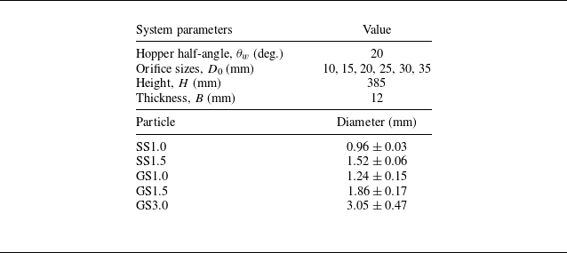


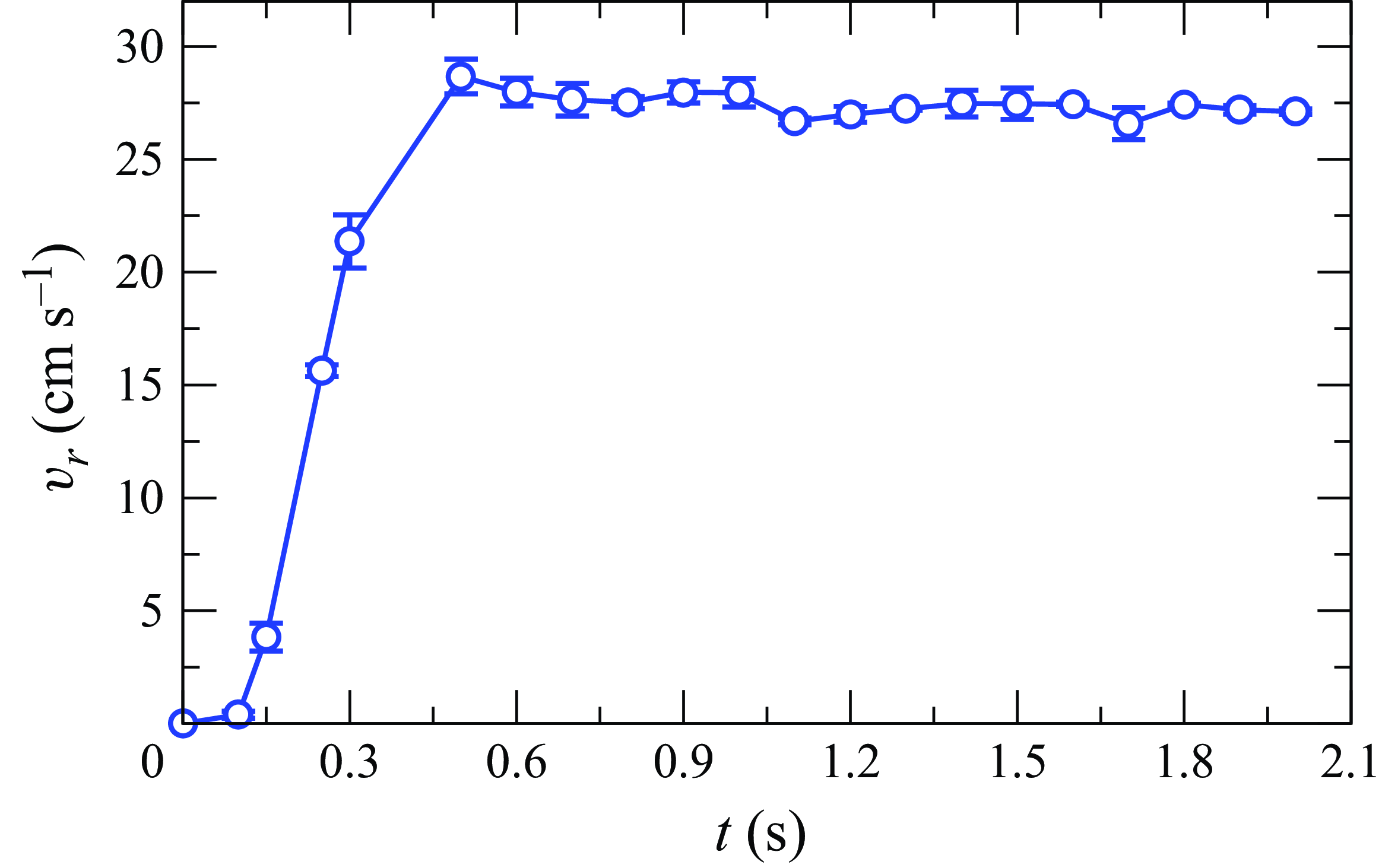


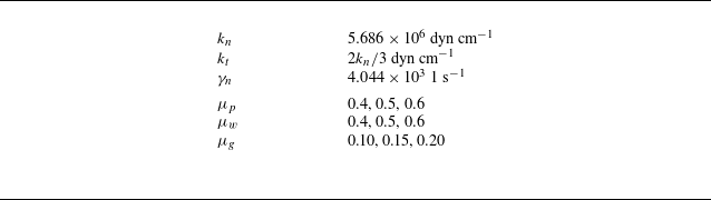


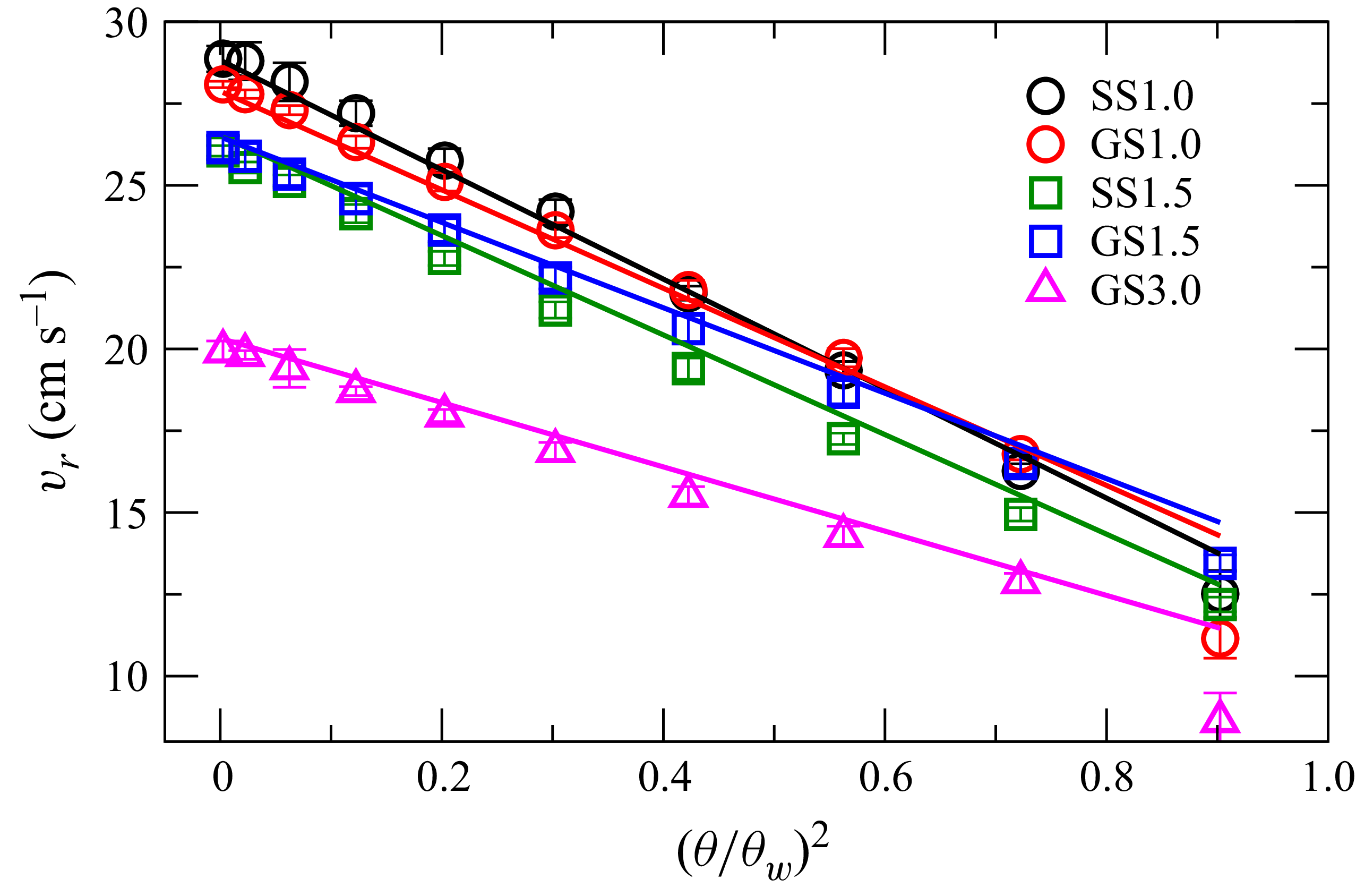


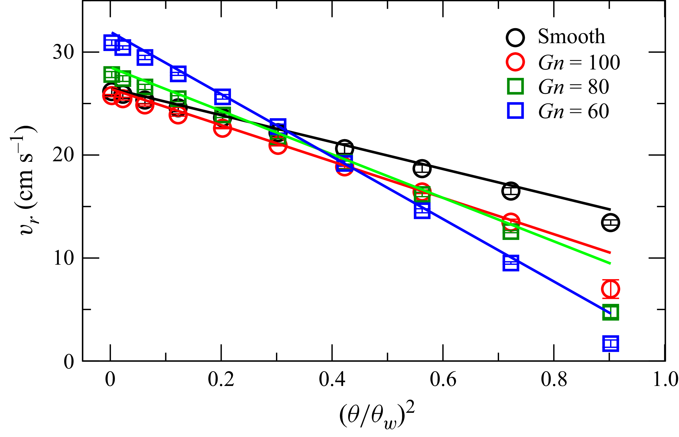


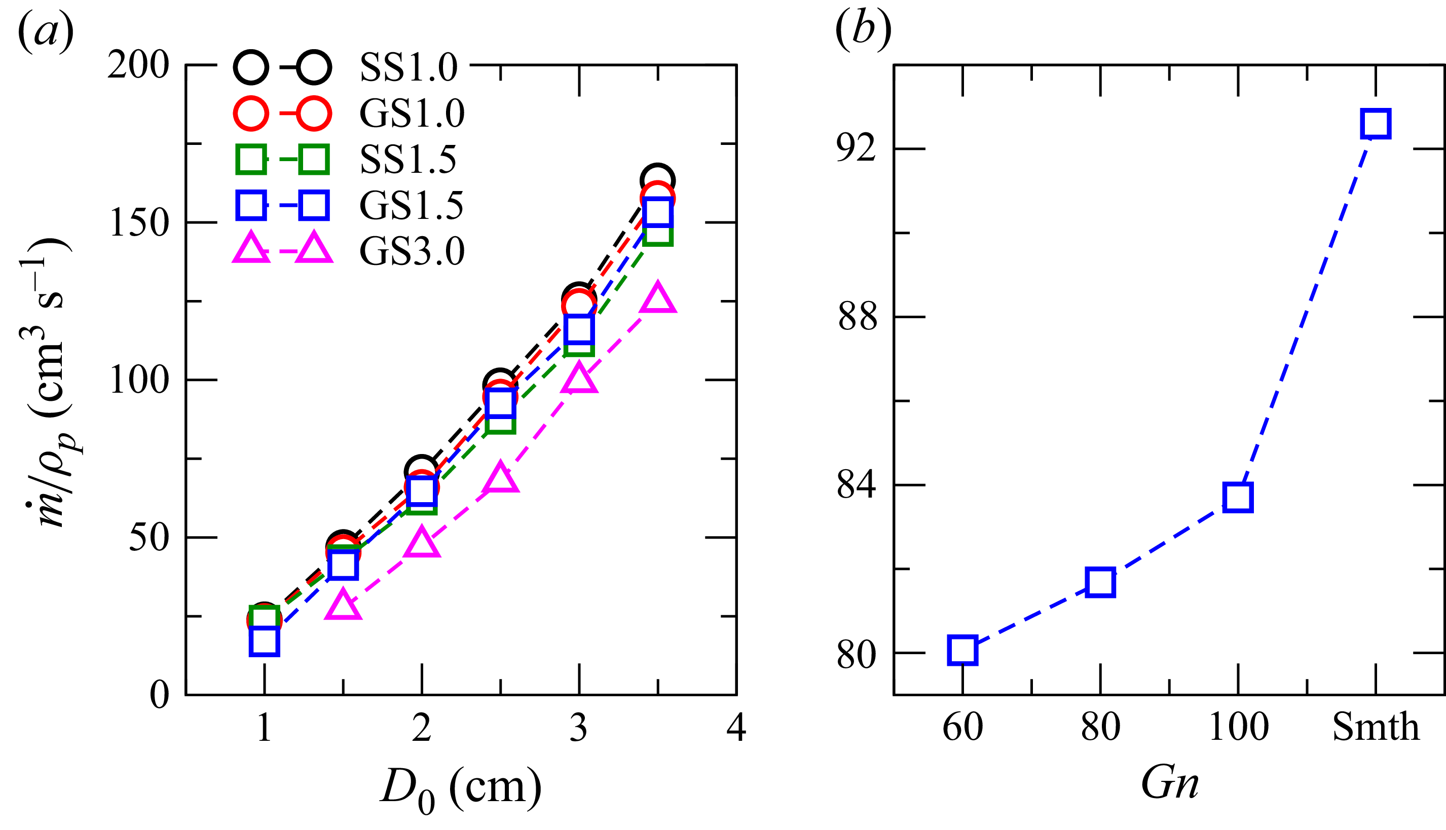


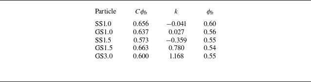
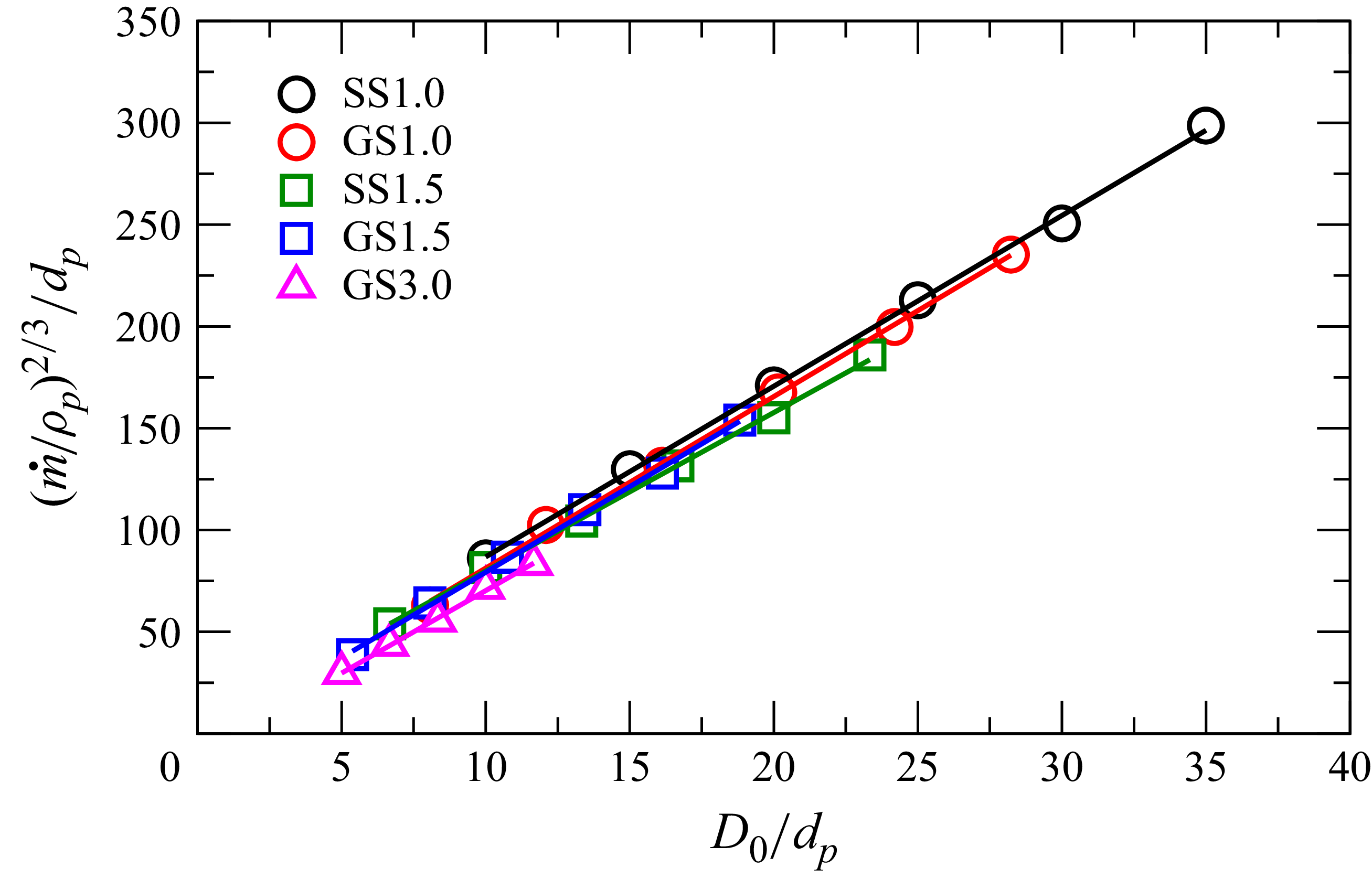


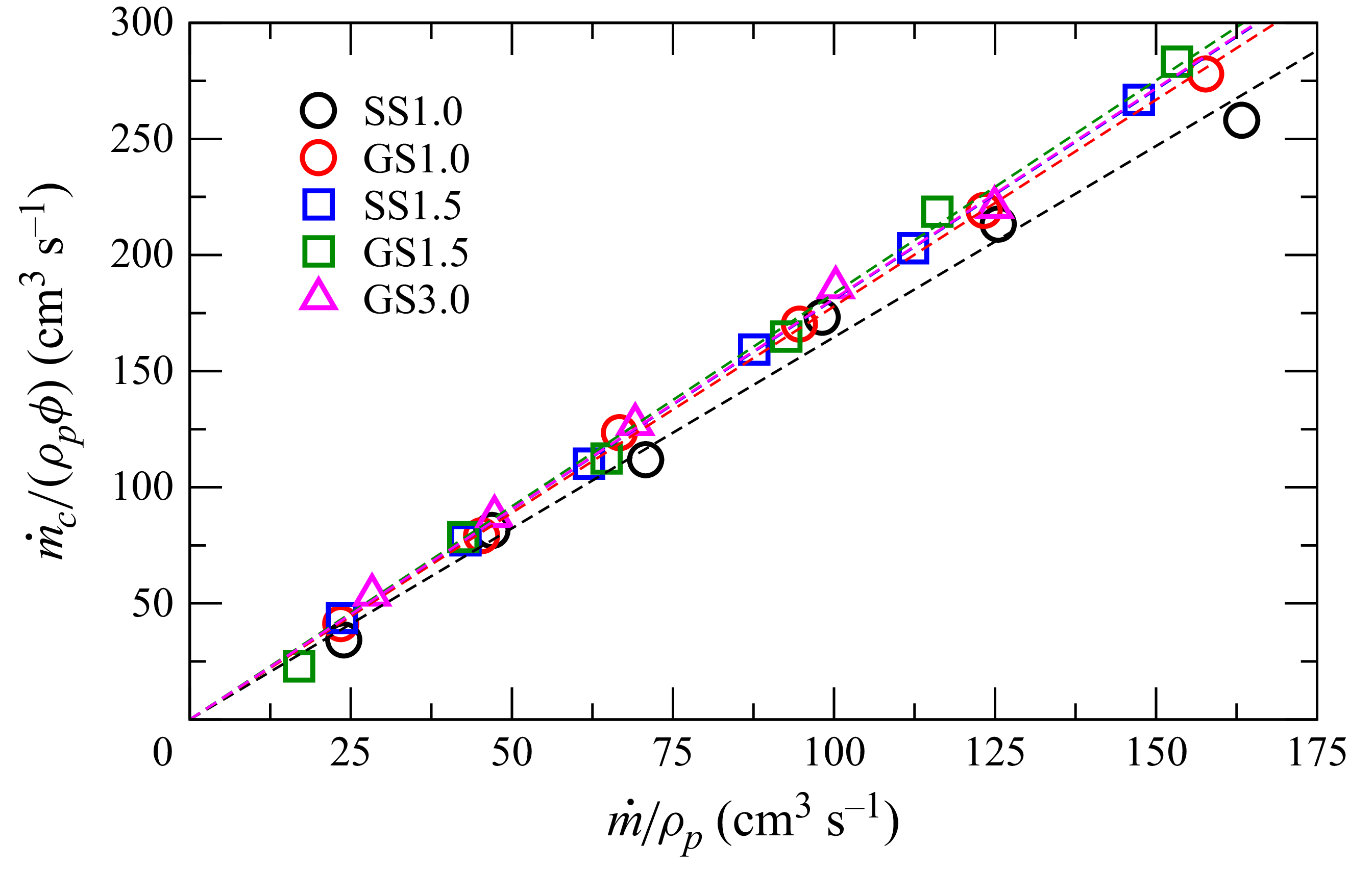


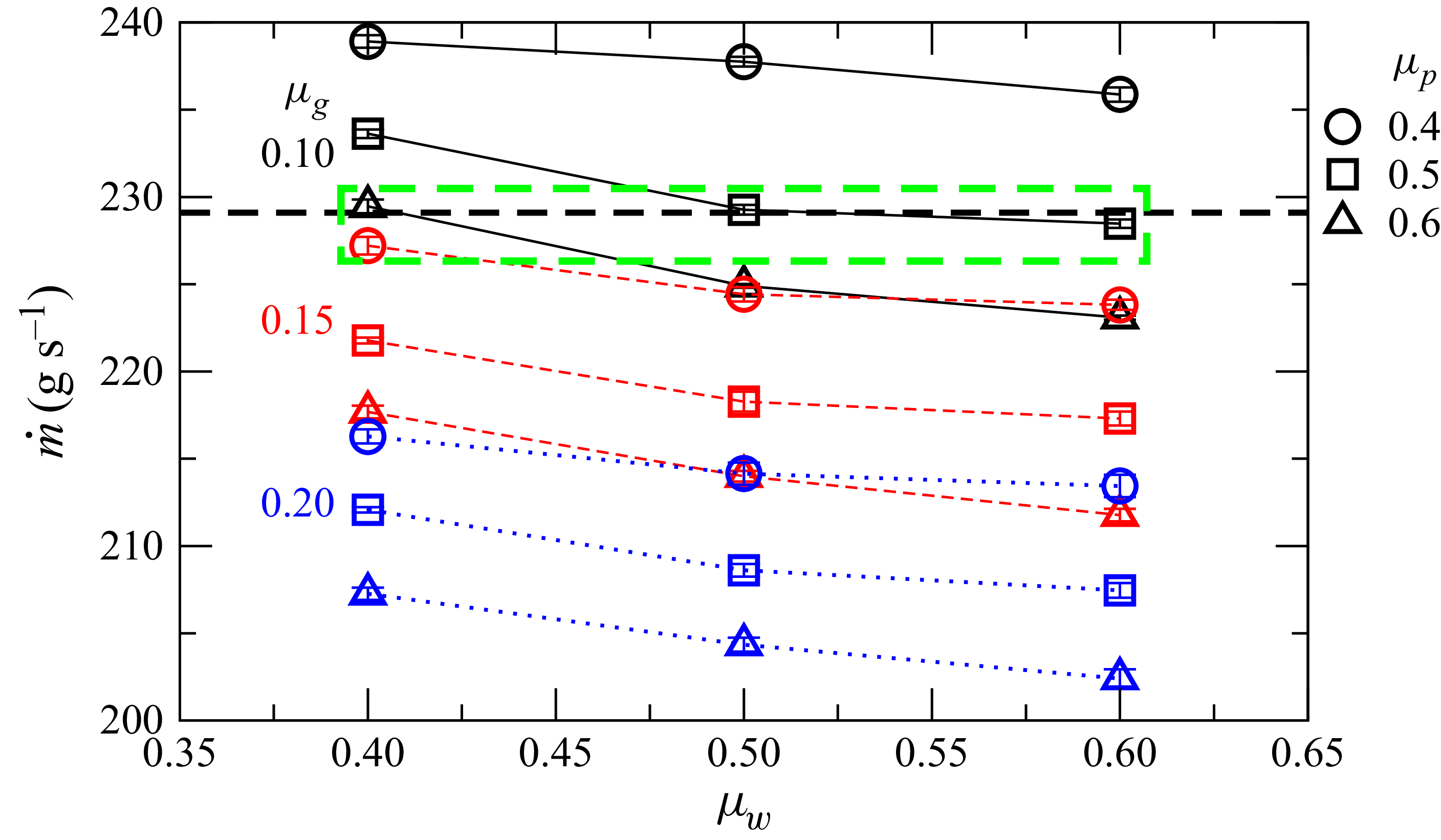


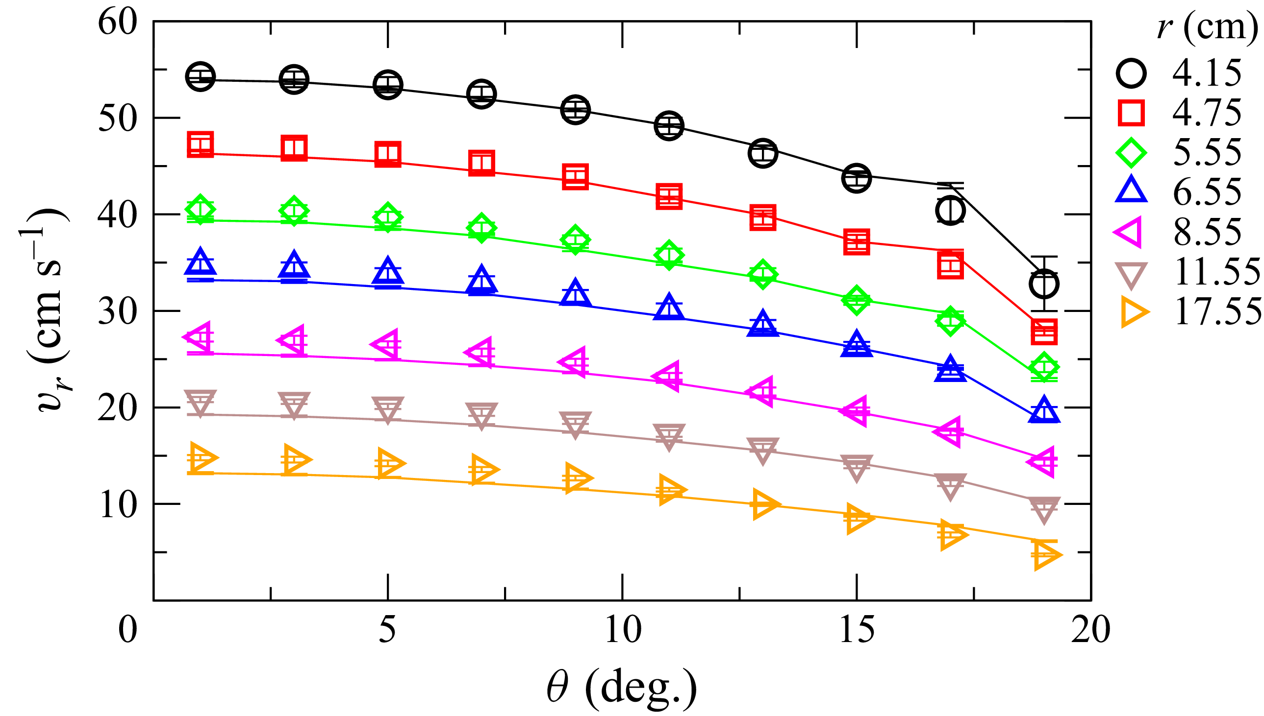


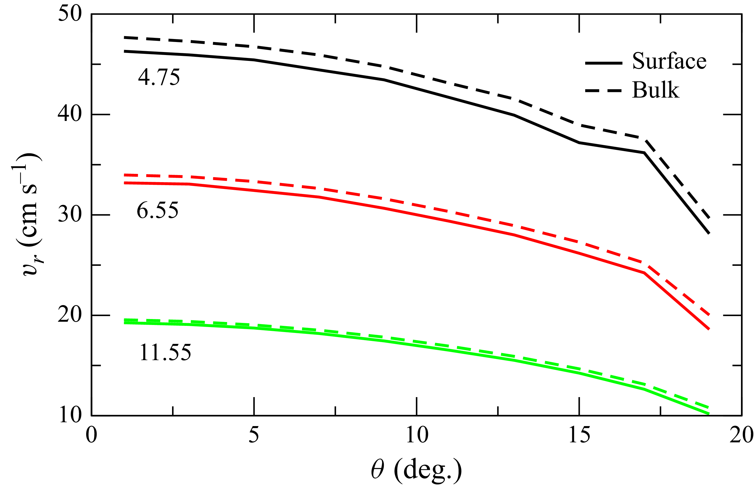


 Open access