2. Problem statement

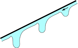
We consider an inverted two-dimensional viscous liquid film that is flowing down the underside of a plane wall that is inclined at an angle $\beta$ to the horizontal, where ${\rm \pi} /2\leq \beta \leq {\rm \pi}$ (see figure 1a). We use Cartesian coordinates $(\tilde x,\tilde y)$, with $\tilde x$ and $\tilde y$ measuring distance along the wall and normal to it, respectively, as shown in the figure. We use tildes to indicate dimensional variables. Assuming that inertia is negligible, the flow is governed by the Stokes momentum and continuity equations, namely

(2.1a,b)\begin{equation} \boldsymbol{0} ={-} \tilde{\boldsymbol{\nabla}} \tilde p + \mu\,\tilde{\nabla}^2 \tilde {\boldsymbol{u}} + \rho \tilde{\boldsymbol{G}},\quad \tilde{\boldsymbol{\nabla}} \boldsymbol{\cdot} \tilde {\boldsymbol{u}} = 0, \end{equation}

where $\tilde p$ and $\tilde {\boldsymbol {u}}=(\tilde u,\tilde v)$ are respectively the pressure and velocity in the liquid film, $\tilde {\boldsymbol {G}} = g (\sin \beta, -\cos \beta )$ is the gravitational acceleration, and $\tilde {\boldsymbol {\nabla }} = (\partial /\partial \tilde x,\partial /\partial \tilde y)$. The dynamic viscosity and density of the fluid are $\mu$ and $\rho$, respectively. The pressure in the air below the film is taken to be zero without loss of generality.

Figure 1.

(a) Schematic representation of a viscous liquid film flow down an inclined plane wall.(b) Schematic for the fixed-volume case showing a drop on a thin precursor film.

At the wall, we have the no-slip condition, $\tilde {\boldsymbol {u}} = \boldsymbol {0}$ at $\tilde y=0$. At the free surface, we must impose the kinematic condition, ${\rm D}\tilde f/{\rm D}\tilde t = 0$, where $\tilde f=0$ describes the location of the free surface, and $\tilde {t}$ denotes time. In the simplest case, the free surface is a graph of a function such that $\tilde f=\tilde y-\tilde h(\tilde x,\tilde t)$, and the kinematic condition takes the form

(2.2)\begin{equation} \tilde v=\tilde h_{\tilde t} + \tilde u\tilde h_{\tilde x}, \end{equation}

at $\tilde y=\tilde h(\tilde x,\tilde t)$. Also, at the free surface, we impose the dynamic stress conditions

(2.3a,b)\begin{equation} \boldsymbol{t}\boldsymbol{\cdot} \tilde{\boldsymbol{T}} \boldsymbol{\cdot} \boldsymbol{n} = 0,\quad \boldsymbol{n}\boldsymbol{\cdot} \tilde{\boldsymbol{T}} \boldsymbol{\cdot} \boldsymbol{n} = \sigma \tilde \kappa, \end{equation}

where $\sigma$ is the surface tension coefficient, and $\boldsymbol {t}$ and $\boldsymbol {n}$ are the unit tangent and unit normal vectors at the free surface, respectively, with $\boldsymbol {n}$ pointing into the liquid. The free surface curvature is given by $\tilde \kappa =\tilde {\boldsymbol {\nabla }}\boldsymbol {\cdot } \boldsymbol {n}$ and is positive/negative as illustrated in figure 1(a), and $\tilde {\boldsymbol {T}}=-\tilde p\boldsymbol {I} + \mu (\tilde {\boldsymbol {\nabla }} \tilde {\boldsymbol {u}} + \tilde {\boldsymbol {\nabla }} \tilde {\boldsymbol {u}}^{\rm T})$ is the Newtonian stress tensor in the liquid (where the superscript ${\rm T}$ denotes matrix transpose).

For a flat film of uniform thickness $h_0$, the velocity field inside the film adopts the unidirectional Nusselt velocity profile with velocity components

(2.4a,b)\begin{equation} \tilde u(\tilde y) = \frac{\rho g \sin \beta}{2\mu}\,(2h_0\tilde y-\tilde y^2),\quad \tilde v = 0. \end{equation}

The associated flow rate is

(2.5)\begin{equation} \tilde q = \frac{\rho g h_0^3 \sin \beta}{3\mu}. \end{equation}

When $\beta ={\rm \pi}$, the film is static and the relevant solutions correspond to a balance between surface tension and gravity, that is, solutions to the YL equation discussed in Appendix A.

According to the definition of $\tilde q$, to maintain the same flow rate for a flat film, the film thickness changes with the inclination angle so that

(2.6)\begin{equation} h_0(\beta) = \frac{h^*}{(\sin\beta)^{1/3}}, \end{equation}

where $h^*=(3\mu \tilde q/\rho g)^{1/3}$ is the flat film thickness that is obtained on a vertical wall so that $h^*=h_0({\rm \pi} /2)$. It is convenient to introduce dimensionless variables that are independent of $\beta$. To do this, we use $h^*$ as the length scale, $2\mu /\rho g h^*$ as the time scale, and $\rho g h^*/2$ as the pressure scale. This reveals the dynamical importance of the dimensionless Bond number

(2.7)\begin{equation} {{Bo}} = \frac{\rho g {h^*}^2}{2\sigma}, \end{equation}

and the dimensionless flow rate

(2.8)\begin{equation} q = \left(\frac{2\mu}{\rho g {h^*}^3}\right) \tilde q = \frac{2}{3}\,h_p^3\sin \beta, \end{equation}

where $\tilde q$ is the dimensional flow rate for a Nusselt film defined in (2.5), and

(2.9)\begin{equation} h_p = \frac{h_0}{h^*}=\frac{1}{(\sin\beta)^{1/3}} \end{equation}

is the dimensionless upstream film thickness. Henceforth we drop the tildes to indicate dimensionless variables. In what follows, we will perform calculations assuming a dimensionless fixed flow rate $q$ at different inclination angles $\beta$, and also calculations in which the flow is assumed to be periodic in $x$ with a fixed volume in each period, again for different inclination angles.

Simplifications can be made in the case when the thickness is small in comparison to the typical length scale of any streamwise variations. This is considered in the next section.

3. Thin-film analysis

Assuming that the length scale of the interfacial deformation $\lambda$ is large compared with $h^*$ (i.e. the so called thin-film parameter $\epsilon =h^*/\lambda$ is small), the film thickness satisfies the model equation, made dimensionless according to the scales given in § 2:

(3.1a–c)\begin{equation} h_t + q_x = 0,\quad q = h^3 P_x,\quad P = \frac{2\sin\beta}{3}\,x - \frac{2\cos\beta}{3}\,h +\frac{1}{3\,{{Bo}}}\,h_{xx}, \end{equation}

where $h(x,t)$ and $q(x,t)$ are the dimensionless film thickness and flow rate, respectively, and $P(x,t)$ represents a combination of the leading-order effects of gravity and surface tension. The latter includes the hydrostatic pressure due to gravity, represented by the first two terms (giving the $x$ and $y$ components, respectively), and the capillary pressure due to surface tension, represented by the third term. Equation (3.1a–c) is derived using systematic asymptotics in Kalliadasis et al. (Reference Kalliadasis, Ruyer-Quil, Scheid and Velarde2011) (see also Tseluiko, Blyth & Papageorgiou Reference Tseluiko, Blyth and Papageorgiou2013), and is valid in the present case of negligible inertia provided that ${{Bo}}=O(\epsilon ^2)$ and $\cot \beta =O(\epsilon ^{-1})$ (Blyth et al. Reference Blyth, Tseluiko, Lin and Kalliadasis2018).

We seek travelling-wave solutions in the form of localised pulses or drops such that the film thickness $h$ becomes constant upstream and downstream. Introducing a moving-frame coordinate via the mapping $x\mapsto x+ c t$, for constant wavespeed $c$, a travelling-wave solution $h(x)$ to (3.1a–c) must satisfy

(3.2)\begin{equation} \left[{-}c h + h^{3} \left( \frac{2\sin \beta}{3} - \frac{2\cos\beta}{3}\,h' + \frac{1}{3{{Bo}}}\,h''' \right)\right]'=0, \end{equation}

where a prime indicates differentiation with respect to $x$. We either fix the dimensionless flow rate $q$, which effectively sets the film thickness upstream and downstream via (2.9), or else fix the volume of fluid over a specified domain $[-L,L]$, that is, we set

(3.3)\begin{equation} \int_{{-}L}^L h \,\mbox{d}\kern0.06em x = V, \end{equation}

for some $V$.

There exists an equivalence between a fixed-$V$ localised droplet solution with a precursor film thickness $h_p(\beta )$ for an angle $\beta$ and a fixed-$q$ solution with upstream film thickness $\hat h_p(\hat \beta )$ for a certain angle $\hat \beta$. This equivalence is established by noting that transforming (3.2) so that

(3.4a–c)\begin{equation} h \mapsto h_p(\beta)\,h, \quad x \mapsto ({-}2\,{{Bo}}\cos \beta)^{{-}1/2}x, \quad c \mapsto \tfrac{1}{3} ({-}8\,{{Bo}} \cos^3\beta)^{1/2}\,h_p^3(\beta)\,c \end{equation}

for the fixed-volume case, and

(3.5a–c)\begin{equation} h \mapsto \hat h_p(\hat \beta)\,h, \quad x \mapsto ({-}2\,{{Bo}}\cos \hat \beta)^{{-}1/2}x, \quad c \mapsto \tfrac{1}{3} ({-}8\,{{Bo}} \cos^3\hat \beta)^{1/2}\,\hat h_p^3(\hat \beta)\,c \end{equation}

for the fixed-flow-rate case leads to the same equation, namely

(3.6)\begin{equation} [{-}c h + h^{3} \left( \gamma + h' + h''' \right)]'=0, \end{equation}

subject to the condition that $h$ approaches unity in the far field, where

(3.7)\begin{equation} \gamma ={-} \frac{\tan \beta}{h_p(\beta)\,({-}2\,{{Bo}} \cos \beta)^{1/2}} ={-} \frac{\tan \hat \beta}{\hat h_p(\hat \beta)\,({-}2\,{{Bo}} \cos \hat \beta)^{1/2}}>0. \end{equation}

The upstream film thickness for the fixed-flow-rate solution is known via (2.8) to be $\hat h_p(\hat \beta )=(3q/2\sin \hat \beta )^{1/3}$, but the precursor film thickness $h_p(\beta )$ for the fixed-volume localised droplet case must be found as part of the solution to the problem. Equation (3.6) was also derived and analysed by Kalliadasis & Chang (Reference Kalliadasis and Chang1994) in a different context, namely drop formation on vertical fibres. They showed that solutions to (3.6) with $h(\pm \infty )=1$ blow up as $c\to \infty$ such that $\gamma \rightarrow \gamma _c\approx 0.5960$. The problem was later revisited by Yu & Hinch (Reference Yu and Hinch2013), who supplied higher-order corrections, noting that $\gamma = \gamma _c + 0.33c^{-2/3} + 0.19c^{-1} + O(c^{-4/3})$. The implications for the present work are: (i) for the fixed-$V$ case,

(3.8)\begin{equation} h_p(\beta) = \frac{{\rm \pi}-\beta}{\gamma_c(2\,{{Bo}})^{1/2}} + o({\rm \pi}-\beta) \end{equation}

as $\beta \to {\rm \pi}-$, and (ii) for the fixed-$q$ case, there is a critical angle, $\hat \beta _c$ say, at which blow-up occurs, that satisfies

(3.9)\begin{equation} \frac{(\sin \hat\beta_c)^{4/3}}{2^{1/6}3^{1/3}q^{1/3}\,{{Bo}}^{1/2}(-\cos \hat \beta_c)^{3/2}} = \gamma_c \approx 0.5960. \end{equation}

A common approximation adopted in the literature is to replace the simplified curvature term in (3.1a–c) with its exact form. Such an approximation is ad hoc, but nevertheless it has been used successfully to predict thin-film flows in a number of different contexts, for example in liquid-film break-up (Gauglitz & Radke Reference Gauglitz and Radke1988). In this case, the thin-film system takes the form (3.1a–c) but with

(3.10)\begin{equation} P = \frac{2\sin\beta}{3}\,x - \frac{2\cos\beta}{3}\,h +\frac{1}{3\,{{Bo}}}\,\kappa, \end{equation}

where

(3.11)\begin{equation} \kappa = \frac{h_{xx}}{(1+h_x^2)^{3/2}} \end{equation}

is the curvature. We will refer to this as the full curvature model (FCM), and we will refer to (3.1a–c) as the linearised curvature model (LCM). Note that there is no equivalence between the cases of fixed flow rate and fixed volume for the FCM. Similarly, there is no such equivalence for the full Stokes system described in § 2.

In the fixed-volume case, our particular interest is in the limit when $\beta \to {\rm \pi}-$ so that the wall tends to become horizontal. Numerical computations, which will be discussed in detail later, indicate that solutions take the form of localised drops with a very thin precursor film on either side, as sketched in figure 1(b). As $\beta$ approaches ${\rm \pi}$, the precursor film thickness tends to zero, and the drop profiles converge to solutions of the YL equation for a static drop that represent a balance between surface tension and gravity. Such solutions are discussed in Appendix A.

Given the aforementioned restrictions, the thin-film models formally break down when $\beta$ is sufficiently close to ${\rm \pi}$. We will subsequently carry out computations for the full equations of Stokes flow with a view to assessing the performance of the thin-film models. This comparison will be presented along with all of our main results in § 6.

4. Asymptotics for $\beta \to {\rm \pi}-$ for fixed volume for the FCM

In this section, we present an asymptotic analysis of the fixed-volume FCM solutions in the limit $\beta \to {\rm \pi}-$. According to the discussion in Appendix A, such an analysis is relevant provided that ${\textit {Bo}}\, V \leq 2.60$ and there exists a limiting static solution (see in particular figure 14). We do not attempt a similar analysis for fixed flow rate since the numerical continuation studies to be presented in a later section indicate the presence of either a turning point or an infinite-slope singularity meaning that the angle $\beta ={\rm \pi}$ is not reached. For the LCM model, the fixed-volume and fixed-flow-rate cases are equivalent, as was noted in § 3, and the analogous asymptotic analysis has been carried out elsewhere (see Kalliadasis & Chang Reference Kalliadasis and Chang1994; Yu & Hinch Reference Yu and Hinch2013).

In a frame of reference travelling at speed $c$ in the positive $x$ direction, writing $z=x-ct$, the FCM (3.10) becomes

(4.1a,b)\begin{equation} -ch_z + q_z = 0,\quad q = h^3 \left(\frac{2\sin\beta}{3} - \frac{2\cos\beta}{3}\,h_z +\frac{1}{3\,{{Bo}}}\,\kappa_z\right), \end{equation}

where the curvature is

(4.2)\begin{equation} \kappa = \frac{h_{zz}}{(1+h_z^2)^{3/2}}, \end{equation}

assuming that the solution is a single-valued function of $z$. Integrating once, we have

(4.3)\begin{equation} -ch + q = Q \end{equation}

for constant $Q$. We introduce the parameter $\delta = {\rm \pi}-\beta$ and henceforth assume that $\delta \ll 1$. The asymptotic solution has the structure depicted in figure 2 and incorporates four regions: the main part of the drop (region $R_2$), the left-side matching zone (region $B_1$), the right-side matching zone (region $B_2$) and the precursor films (regions $R_1$ and $R_3$).

Figure 2.

Sketch of the asymptotic regions for the case of fixed volume.

In region $R_2$, we expand by writing

(4.4a–c)\begin{align} h=h_0(z) + \delta\,h_1(z) + \delta^{3/2}\,h_2(z) + \cdots,\quad c = \delta^{3/2}c_0 + \cdots,\quad Q = \delta^{5/2} Q_0 + \cdots, \end{align}

where the forms of the expansions have been selected to allow a consistent match between the regions. The inherent degeneracy in the problem due to a translational invariance in $z$ is removed by pinning the drop with its maximum at the origin so that $h'(0)=0$, where a prime denotes differentiation with respect to $z$.

Substituting (4.4a–c) into (4.3) and integrating the leading-order equation once, we obtain

(4.5)\begin{equation} 2 h_0 + \frac{1}{{{Bo}}}\,\frac{h_{0}''}{(1+h_0'^2)^{3/2}} = P_0, \end{equation}

where $P_0$ is a constant of integration. The solution $h_0(z)$ is a static-drop at $\beta ={\rm \pi}$ with the support from $-\ell$ to $\ell$. It touches the wall with zero slope at the ends so that $h_0(\pm \ell ) = h_0'(\pm \ell )=0$, and has volume $V$ so that

(4.6)\begin{equation} \int_{-\ell}^\ell h_0(z)\,{\rm d} z = V, \end{equation}

and the volume contained in each of $h_1$, $h_2$, etc. is zero. This solution is analysed in Appendix A. With the pinning condition $h_0'(0)=0$, we have

(4.7)\begin{equation} h_0 \sim a_0 (z \pm \ell)^2 \quad \mbox{as}\ z\to \mp \ell, \end{equation}

where the coefficient $a_0$ can be estimated from the numerical solution and depends on $V$. The solution for the case $V=8$ and ${\textit {Bo}}=0.3$ is shown in figure 3(a) and is such that $\ell =3.3598$ and $a_0=0.3572$.

Figure 3.

For $V=8$ and ${\textit {Bo}}=0.3$: (a) leading-order solution $h_0(z)$; (b) the functions $h_{1O}(z)$ and $h_{1P}(z)$.

At $O(\delta )$, we find after one integration,

(4.8)\begin{equation} (2\,{{Bo}}) h_{1}' + \left( \frac{h_1'}{(1+h_0'^2)^{3/2}} \right ) '' ={-} 2\,{{Bo}}. \end{equation}

The solution can be written in the form

(4.9)\begin{equation} h_1(z) = b_1\,h_{1E}(z) + b_2\,h_{1O}(z) + b_3 + h_{1P}(z), \end{equation}

for constants $b_1$, $b_2$, $b_3$, where $h_{1E}(z)$ and $h_{1O}(z)$ are even and odd functions, respectively, and the particular integral $h_{1P}(z)$ is odd. We assume without loss of generality that $h_{1E}(0)=1$, $h_{1O}'(0)=1$ and $h_{1P}'(0)=1$. Numerically computed solutions for $h_{1O}(z)$ and $h_{1P}(z)$ are shown in figure 3. Restricting attention to the range $[0,\ell ]$, since $h_0(z)$ is symmetric about the inflection point at $z=\ell /2$ (see Appendix A), $h_{1O}(z)$ is also symmetric about the line $z=\ell /2$. The pinning condition $h_1'(0)=0$ demands that $b_2=-1$. Hence

(4.10)\begin{equation} h_1(\ell) - h_1(-\ell) = 2h_{1P}(\ell). \end{equation}

From our numerical solution, we determine that $h_{1P}(\ell ) = -3.3740$.

At $O(\delta ^{3/2})$, we find

(4.11)\begin{equation} (2\,{{Bo}}) h_2' + \left( \frac{h_2'}{(1+h_0'^2)^{3/2}} \right )'' = \frac{3c_0\,{{Bo}}}{h_0^2}. \end{equation}

The solution has the singular behaviour

(4.12)\begin{equation} h_2 \sim{-}\frac{c_0\,{{Bo}}}{2a_0^2}\,(z\pm \ell)^{{-}1} \end{equation}

as $z\to \mp \ell$, signalling a breakdown in the expansion (4.4a–c) in region $R_2$ where $z\pm \ell = O(\delta ^{1/2})$, thus necessitating the regions $B_1$ and $B_2$ to be discussed below.

In regions $R_1$ and $R_3$, we expand by writing

(4.13)\begin{equation} h = \delta h_{p0} + \cdots. \end{equation}

Substituting into (4.3), we obtain at leading order $-c_0 h_{p0} = Q_0$. In region $B_1$, we write $(z+\ell ) = \delta ^{1/2}\xi$, where $\xi =O(1)$, and expand by writing $h = \delta \,H_0(\xi ) + \cdots$. Substituting into (4.1a,b) and integrating once, we obtain

(4.14)\begin{equation} H_0^3H_{0\xi\xi\xi} - c_0H_0 = Q_0. \end{equation}

Matching with regions $R_1$ and $R_2$ requires that

(4.15a,b)\begin{equation} H_0 \sim h_{p0} \mbox{ as } \xi \to -\infty,\quad H_0 \sim a_0\xi^2 + h_1({-}L) - \frac{c_0\,{{Bo}}}{2a_0^2}\,\xi^{{-}1} \mbox{ as } \xi \to \infty, \end{equation}

respectively. Here, $h_{p0}$ is the scaled leading-order precursor film thickness to be determined. If we rescale by writing $\xi = (h_{p0}/c_0^{1/3})\zeta$, $H_0(\xi ) = h_{p0}\,F(\zeta )$, then the problem takes the form (see also Bretherton Reference Bretherton1961)

(4.16)\begin{equation} F^3 F_{\zeta\zeta\zeta} - F + 1 = 0, \end{equation}

with

(4.17a,b)\begin{equation} F \sim 1 \mbox{ as } \zeta \to -\infty,\quad F \sim \mu_0 \zeta^2 + \mu_1\zeta + \mu_2 \mbox{ as } \zeta \to \infty, \end{equation}

where $\mu _0 = a_0h_{p0}/c_0^{2/3}$, and $\mu _1,\mu _2$ are constants to be found. Useful insight is obtained by reformulating the problem as the first-order system $(u_1,u_2,u_3)_\zeta = (u_2,u_3,u_1^{-2} - u_1^{-3})$, with $(u_1,u_2,u_3)=(F,F_\zeta,F_{\zeta \zeta })$. It is straightforward to show that the fixed point at $(1,0,0)$ has a one-dimensional unstable manifold and a two-dimensional stable manifold. Thus, if it exists, the solution that fulfils the boundary conditions (4.17a,b) is unique up to a translation in $\zeta$. This freedom allows us to fix $\mu _1=0$ so as to satisfy (4.15a,b) and match with region $R_2$. Solving numerically, we determine that $\mu _0 = 0.3215$ and $\mu _2 = 2.8996$, in exact agreement with the values calculated by Yu & Hinch (Reference Yu and Hinch2013). The numerical solution is shown in figure 4.

Figure 4.

(a) Solution $F(y)$ to the problem (4.16), (4.17a,b). (b) Solution $G(Y)$ to the problem (4.19), (4.20a,b).

Similar scalings apply in region $B_2$. Writing $z-\ell = \delta ^{1/2}\tilde \xi$ and $h = \delta \,\tilde H_0(\tilde \xi ) + \cdots$, the leading-order equation is found to be identical to (4.14) but with tildes over all of the symbols except $c_0$. Matching to regions $R_2$ and $R_3$ requires that

(4.18a,b)\begin{equation} \tilde H_0 \sim a_0 \tilde \xi^2 + h_1(\ell) - \frac{c_0\,{{Bo}}}{2a_0^2}\,\tilde \xi^{{-}1} \mbox{ as } \tilde\xi \to -\infty,\quad \tilde H_0 \to h_{p0} \mbox{ as } \tilde \xi \to \infty, \end{equation}

respectively. Rescaling so that $\tilde \xi = (h_{p0}/c_0^{1/3})Y$, $\tilde H_0(\tilde \xi ) = h_{p0}\,G(Y)$, we have

(4.19)\begin{equation} G^3G_{YYY} - G + 1 = 0, \end{equation}

with

(4.20a,b)\begin{equation} G \sim \mu_0 Y^2 + \nu_1 Y + \nu_2 + \cdots \mbox{ as } Y \to -\infty,\quad G \sim 1 \mbox{ as } Y \to \infty, \end{equation}

for constants $\nu _1,\nu _2$. The translational invariance with respect to $Y$ affords the freedom to set $\nu _1=0$ as required by the match with region $R_2$ via (4.18a,b).

Recasting as a first-order system, it is readily seen that the fixed point at $(G,G_Y,G_{YY})=(1,0,0)$ has a two-dimensional stable manifold, indicating that (4.19)–(4.20a,b) have a one-parameter family of solutions for $G(Y)$. The numerical solution, for which $\mu _0$ is set to the value computed above in region $B_1$, determines that $\nu _2 = -0.8453$. This is in exact agreement with the value given by Yu & Hinch (Reference Yu and Hinch2013).

Using the above results, we have that $h_1(-\ell ) = \mu _2 h_{p0}$ and $h_1(\ell ) = \nu _2 h_{p0}$. Then using (4.10), we obtain the value of the scaled leading-order precursor film thickness,

(4.21)\begin{equation} h_{p0} = \frac{2\,h_{1P}(\ell)}{\nu_2-\mu_2} = 1.80, \end{equation}

and the leading-order wave speed coefficient

(4.22)\begin{equation} c_0 = \left( \frac{a_0h_{p0}}{\mu_0}\right)^{3/2} = 2.83. \end{equation}

5. Travelling-wave computational method for Stokes flow

The thin-film models are formally restricted to small Bond numbers and the requirement that $\cot \beta = O(\epsilon ^{-1})$, as discussed in § 3. The latter condition means that the thin-film model breaks down when $\beta$ is sufficiently close to ${\rm \pi}$ and the inverted wall is almost horizontal. In § 6, we will present results based on the thin-film models for angles $\beta$ that are very close to ${\rm \pi}$, and also for large-amplitude surface deformations. To allow us to corroborate these calculations, we herein extend the discussion to parameter regimes beyond the range of validity of the thin-film models, and present a numerical boundary-integral method for computing travelling waves in Stokes flow (see, for example, Pozrikidis (Reference Pozrikidis1992) for a discussion of the theoretical formulation for such methods).

We work in a frame of reference that is travelling with the wave at speed $c$. Here and henceforth, all variables have been made dimensionless according to the scales mentioned in § 2. We decompose the velocity field in the fluid by writing

(5.1)\begin{equation} \boldsymbol{u} = (\boldsymbol{U}(y) - c\boldsymbol{i}) + \bar{\boldsymbol{u}}(\boldsymbol{x},t), \end{equation}

where $\boldsymbol {U} = (u,v)$ is the dimensionless form of the Nusselt solution (2.4a,b), $\boldsymbol {i}$ is the unit vector in the $x$ direction, and $\bar {\boldsymbol {u}}$ is the disturbance field that vanishes at the wall and is to be found. The fluid stress $\boldsymbol {f}$ at a point $(x,y)$ on the free surface is similarly split up so that $\boldsymbol {f} = \boldsymbol {F} + \bar {\boldsymbol {f}}$, where $\boldsymbol {F}$ is the dimensionless Nusselt stress given by

(5.2)\begin{equation} \boldsymbol{F} ={-}2\cos \beta\,(\sin^{{-}1/3}\beta - y) \boldsymbol{n} + 2\sin \beta\,(\sin^{{-}1/3}\beta - y) \begin{pmatrix} 0 & 1\\ 1 & 0 \end{pmatrix}\boldsymbol{n}, \end{equation}

and $\boldsymbol {n}$ is the unit normal vector at the surface pointing into the fluid.

The disturbance velocity and traction fields satisfy the Fredholm integral equation of the second kind for the disturbance velocity,

(5.3)\begin{equation} 2{\rm \pi}\,\bar{u}_j(\boldsymbol{x}_0) ={-}S_j(\boldsymbol{x}_0) + D_j(\boldsymbol{x}_0), \end{equation}

for $j=1,2$ at a point $\boldsymbol {x}_0=({x}_0,{y}_0)$ that is located on the free surface, labelled $\mathscr {C}$, where

(5.4a,b)\begin{align} S_j(\boldsymbol{x}_0) = \int_{\mathscr{C}} G_{ij}(\boldsymbol{x},\boldsymbol{x}_0)\,\bar{f}_i(\boldsymbol{x})\,\mbox{d} s(\boldsymbol{x}), \quad D_j(\boldsymbol{x}_0) = \int_{\mathscr{C}}^{\mathrm{p.v.}} \bar{u}_i(\boldsymbol{x})\,T_{ijk}(\boldsymbol{x},\boldsymbol{x}_0)\,n_k(\boldsymbol{x})\,\mbox{d} s(\boldsymbol{x}) \end{align}

are the single-layer and double-layer potentials, respectively, and where p.v. denotes the principal value. In (5.4a,b), $s$ is arc length along the free surface $\mathscr {C}$, and $G_{ij}(\boldsymbol {x},\boldsymbol {x}_0)$ and $T_{ijk}(\boldsymbol {x},\boldsymbol {x}_0)$ are suitable choices for the Green's function and the stress tensor, respectively, for singularly forced Stokes flow. In the travelling frame, the kinematic condition requires that the normal component of velocity on the free surface vanishes, so that $\boldsymbol {u}\boldsymbol {\cdot } \boldsymbol {n}=0$, and therefore

(5.5)\begin{equation} \bar{\boldsymbol{u}} = u^{(t)}\boldsymbol{t} -\boldsymbol{U} + c\boldsymbol{i} \end{equation}

on $\mathscr {C}$, where $u^{(t)}=\boldsymbol {u}\boldsymbol {\cdot } \boldsymbol {t}$ is the a priori unknown tangential component of the total fluid velocity at the free surface, and $\boldsymbol {t}$ is the unit tangent pointing in the direction of increasing arc length.

The dynamic stress conditions (2.3a,b) demand that $\boldsymbol {t}\boldsymbol {\cdot } \boldsymbol {f} = 0$ and $\boldsymbol {n}\boldsymbol {\cdot } \boldsymbol {f} = {\textit {Bo}}^{-1}\,\kappa$ on $\mathscr {C}$, and hence that

(5.6)\begin{equation} \bar{\boldsymbol{f}} = {{Bo}}^{{-}1}\,\kappa \boldsymbol{n} - \boldsymbol{F} \end{equation}

on $\mathscr {C}$, where $\boldsymbol {F}$ was given in (5.2). Here, the curvature is $\kappa = -\boldsymbol {n}\boldsymbol {\cdot } \boldsymbol {t}_s$, where the subscript $s$ denotes a derivative with respect to arc length. This definition is consistent with that made in § 2.

The integral equation (5.3) together with the kinematic condition (5.5) and the dynamic stress conditions (5.6) must be solved numerically. We work on a computational domain with periodic boundary conditions, and we use the periodic Green's function $\boldsymbol {G}^{{\rm{PW}}}$ that has the property $\boldsymbol {G}^{{\rm{PW}}}(\boldsymbol {x},\boldsymbol {x}_0)=\boldsymbol {0}$ when $\boldsymbol {x}$ lies on the wall at $y=0$ (see, for example, Pozrikidis Reference Pozrikidis1992):

(5.7)\begin{equation} \boldsymbol{G}^{{{\rm PW}}}(\boldsymbol{x},\boldsymbol{x}_0) = \boldsymbol{G}^{{{\rm P}}}(\hat{\boldsymbol x}) - \boldsymbol{G}^{{{\rm P}}}(\hat{\boldsymbol X}) + 2{y}_0^2\,\boldsymbol{G}^{{{\rm DP}}}(\hat{\boldsymbol X}) -2{y}_0\,\boldsymbol{G}^{{{\rm SDP}}}(\hat{\boldsymbol X}), \end{equation}

where $\hat {\boldsymbol x}=\boldsymbol {x}-\boldsymbol {x}_0$, and $\boldsymbol {X}=\boldsymbol {x}-\boldsymbol {x}_0'$, with $\boldsymbol {x}_0'=({x}_0,-{y}_0)$. In (5.7), the Green's function

(5.8)\begin{equation} \boldsymbol{G}^{{{\rm P}}}({\boldsymbol{x}}) = \begin{pmatrix} 1 - A - yA_{ y} & yA_{ x} \\ yA_{ x} & yA_{ y}-A \end{pmatrix}, \end{equation}

where

(5.9)\begin{equation} A(\boldsymbol{x}) = \tfrac{1}{2}\log\left(\cosh (2{\rm \pi} y/L) - \cos (2{\rm \pi} x/L)\right) + \tfrac{1}{2}\log 2 \end{equation}

corresponds to a periodic array of Stokeslets, with $A_x,A_y$ denoting derivatives, and $\boldsymbol {G}^{{{\rm DP}}}$, $\boldsymbol {G}^{{{\rm SDP}}}$ the periodic potential dipole and periodic Stokeslet doublet, respectively, both given in closed form in Pozrikidis (Reference Pozrikidis1992). An alternative form for the Green's function and stress tensor, derived using a complex variable approach, was provided recently by Crowdy & Luca (Reference Crowdy and Luca2019).

We compute the solution to the integral equation (5.3) with spectral accuracy by adapting the protocol proposed by Veerapaneni et al. (Reference Veerapaneni, Gueyffier, Zorin and Biros2009) for the motion of vesicles in a Stokes flow. We describe a point $\boldsymbol {x}(\alpha )=( x(\alpha ), y(\alpha ))$ on the free surface, and the tangential surface velocity in the form

(5.10a,b)\begin{equation} \boldsymbol{x}(\alpha) = \frac{\alpha L}{\rm \pi}\,\boldsymbol{i} + \sum_{n={-}N}^{N} \hat{\boldsymbol x}_n\,\mbox{e}^{\mathrm{i} n \alpha},\quad u^{(t)}(\alpha) = \sum_{n={-}N}^{N} \hat u_n\,\mbox{e}^{\mathrm{i} n \alpha}, \end{equation}

where $2L$ is the domain size, $\alpha \in [0,2{\rm \pi} )$ is a parameter, $\hat {\boldsymbol x}_n$ and $\hat u_n$ are complex coefficients to be found, $N$ is a specified truncation level, and $\boldsymbol {i}$ is the unit vector in the $x$ direction. Since $\boldsymbol {x}$ and $u^{(t)}$ are real, $\hat {\boldsymbol x}_n=\hat {\boldsymbol x}_{-n}^*$ and $\hat u_n = \hat u_{-n}^*$, where the asterisk denotes the complex conjugate.

Inserting (5.5) and (5.6) into (5.3), we enforce the resulting integral equation at a set of $2N+1$ equally-spaced collocation points $\boldsymbol {x}_0=\boldsymbol {x}(\alpha _0)$, where $\alpha _0 \in \{2(k-1){\rm \pi} /(2N+1): k=1,\ldots,2N+1\}$. The necessary $\alpha$ derivatives are computed at each collocation point using a fast Fourier transform to yield numerical approximations for the unit normal and tangent vectors, and for the free-surface curvature. The single-layer potential $S_j({\boldsymbol {x}_0})$ is weakly singular as $\boldsymbol {x}\to \boldsymbol {x}_0$, and in particular, the Green's function and stress tensor tend toward the two-dimensional Stokeslet

(5.11a,b)\begin{equation} G^{{{\rm ST}}}_{ij} ={-}\delta_{ij}\log {r} + \frac{\hat x_i\hat x_j}{{r}^2},\quad T^{{{\rm ST}}}_{ijk} ={-}4\,\frac{\hat x_i\hat x_j\hat x_k}{{r}^4}, \end{equation}

where $r=|\boldsymbol {x}-\boldsymbol {x}_0|$. The integrand of the single-layer potential is therefore logarithmically singular in this limit and, following Veerapaneni et al. (Reference Veerapaneni, Gueyffier, Zorin and Biros2009), we calculate it numerically with spectral accuracy using the hybrid Gauss-trapezoidal quadrature formula of Alpert (Reference Alpert1999). This hybrid formula assumes the presence of a logarithmic singularity at the lower integration limit, and applies the usual trapezoidal rule in the centre of the integration range, with a weighted Gaussian quadrature at each end. Specifically, it supplies the approximation

(5.12)\begin{align} \mathcal{S}_{ij}(\alpha_0) \approx \omega \sum_{k=1}^{N_L} w^{L}_k\,S_{ij}(v^{L}_k \omega,\alpha_0) + \omega \sum_{k=0}^{N_T} S_{ij}(a\omega + k\omega,\alpha_0) + \omega \sum_{k=1}^{N_R} w^{R}_k\,S_{ij}(v^{R}_k \omega,\alpha_0), \end{align}

where the $w_k$ and $v_k$ with $L$/$R$ superscripts are $N_L,N_R$ weights and nodes at the left-hand and right-hand ends, respectively; $N_T$ is the number of trapezium rule points with spacing $\omega =1/(N_T+a+b-1)$, where $a$ and $b$ are parameters that are related to the convergence properties of the quadrature. In our calculations, we took $a=10$ and $b=7$ with $N_L=15$ and $N_R=8$ to achieve convergence of $O(\omega ^{16}\log \omega )$ (see tables 6 and 8 of Alpert (Reference Alpert1999), where numerical values for the weights and nodes are given). As suggested by Veerapaneni et al. (Reference Veerapaneni, Gueyffier, Zorin and Biros2009), we split the integration of the single-layer potential into the ranges $[0,\alpha _0]$ and $[\alpha _0,2{\rm \pi} ]$, and apply the quadrature rule (5.12) appropriately over each range. For the double-layer potential, we apply the regular quadrature rule of Alpert (Reference Alpert1999), which is obtained by setting $a=b$ and using the same weights and nodes at both ends in (5.12); in this case, we took $a=7$ to achieve $O(\omega ^{16})$ convergence (see table 6 of Alpert Reference Alpert1999).

Next, we express the boundary integral equation (5.3) in the form $\boldsymbol{\mathcal{R}} \equiv 2{\rm \pi} \boldsymbol{\overline{u}} + \boldsymbol{\mathcal{S}} - \boldsymbol{\mathcal{D}} = \boldsymbol{0}$ and we enforce the conditions

(5.13a,b)\begin{equation} \boldsymbol{\mathcal{R}}\boldsymbol{\cdot} \boldsymbol{n} = 0,\quad \boldsymbol{\mathcal{R}}\boldsymbol{\cdot} \boldsymbol{t} = 0 \end{equation}

at the $2N+1$ collocation points ${\boldsymbol {x}}_0={\boldsymbol {x}}(\alpha _0)$ defined above, yielding $4N+2$ algebraic equations. A further $2N$ equations follow by demanding

(5.14)\begin{equation} \int_0^{2{\rm \pi}} |{\boldsymbol{x}}_\alpha|\,\mbox{e}^{\mathrm{i} n\alpha}\,\mbox{d} \alpha = 0 \end{equation}

for $n=\pm 1, \pm 2,\ldots, \pm N$, so that $s_\alpha = |{\boldsymbol {x}}_\alpha |$ is constant along $\mathscr {C}$, and the collocation points are equally spaced with respect to arc length along the free surface. Here, the $\alpha$ subscript denotes a derivative. One further equation arises by fixing the origin in $x$, specifically by setting $x(0)=-L$. The final equation needed is supplied either by fixing the height of the film at one end of the domain in the case of a fixed-flow-rate calculation, setting $y(0)=h_0$, or else by fixing the fluid volume as

(5.15)\begin{equation} \int_{{-}L}^L y\, \mbox{d}\kern0.06em x = \int_0^{2{\rm \pi}} y x_{\alpha}\,\mbox{d} \alpha = V. \end{equation}

The translational invariance of the system is removed by fixing the free-surface maximum to lie in the middle of the domain, setting

(5.16)\begin{equation} y_\alpha({\rm \pi}) = 0. \end{equation}

For any $\boldsymbol {x}_0$, conservation of mass implies that (Pozrikidis Reference Pozrikidis1992)

(5.17)\begin{equation} \int_{\mathscr{C}} G^{{{\rm PW}}}_{ij}(\boldsymbol{x},\boldsymbol{x}_0)\,n_j(\boldsymbol{x})\,\mbox{d} s(\boldsymbol{x}) = 0, \end{equation}

so, referring to (5.3), the disturbance stress $\bar {\boldsymbol {f}}$ is determined to within an arbitrary constant multiple of $\boldsymbol {n}$. Consequently, one equation can be removed arbitrarily from the projection $\boldsymbol {\mathcal {R}}\boldsymbol {\cdot } \boldsymbol {n}=0$ in (5.13a,b) to obtain a system of $6N+4$ equations for the $6N+4$ unknowns comprising the $6N+3$ Fourier coefficients $\{\hat {\boldsymbol x}_n,\hat u_n\}$, and $c$. This system is solved using Newton's method, wherein at each stage we compute the Fourier representation (5.10a,b) using a fast Fourier transform.

6. Numerical results

In this section, we study the behaviour of steady pulse solutions in the two cases of fixed flow rate and fixed volume. Of particular interest is to follow the solution branch for a pulse as $\beta$ increases and the wall tends to become horizontal, a limit that we naturally associate, on the basis of physical intuition, with the onset of dripping.

Working on a periodic domain $[-L,L]$, we compute travelling-wave solutions to the long-wave LCM and FCM equations introduced in § 3 using a scheme based on Newton iterations and a Fourier pseudo-spectral representation of the spatial derivatives (see Blyth et al. Reference Blyth, Tseluiko, Lin and Kalliadasis2018; Lin et al. Reference Lin, Tseluiko, Blyth and Kalliadasis2018), and to the equations of Stokes flow using the numerical method discussed in § 5. Travelling-wave solution branches emerge from the neutral stability point where the growth rate of small-amplitude periodic waves vanishes. The relationship between $\beta$, ${{Bo}}$ and $L$ at the neutral stability point is

(6.1)\begin{equation} L = {\rm \pi}({-}2\,{{Bo}} \cos\beta)^{{-}1/2} \end{equation}

for both the LCM and the FCM (see Blyth et al. Reference Blyth, Tseluiko, Lin and Kalliadasis2018), and for Stokes flow (see Appendix C). For a chosen ${{Bo}}$, we fix the domain size $2L$ and calculate the inclination angle close to the critical value determined from (6.1) to compute a small-amplitude periodic wave. We then perform pseudo-arc-length continuation in $\beta$ to study localised drop formation as the wall tends to become horizontal.

In the following subsections, we study the cases of fixed volume $V$ and fixed flow rate $q$ separately. Throughout, we will refer to the maximum vertical distance between the wall and the film surface (measured in the $y$ direction, as depicted in figure 1) as the drop height $H$, and we will use it as a measure of the solutions in the bifurcation diagrams that we will construct. In each case, we consider computations at the small Bond number ${{Bo}}=0.005$ in order to facilitate comparison between the long-wave models and Stokes flow, as well as the larger Bond number ${{Bo}}=0.3$ in order to study the dynamics beyond the range of validity of the long-wave models. In the case of fixed volume, for each Bond number we select a couple of cases wherein ${\textit {Bo}}\,V$ is before and after the turning point in figure 14. Specifically, we choose $V=400$ and $900$ for the case ${\textit {Bo}}=0.005$, and we choose $V=8$ and $15$ for the case ${\textit {Bo}}=0.3$ (see table 1). For fixed flow rate, for each of the two Bond numbers we set $q=2/3$ as required by the non-dimensionalisation, which demands a film of unit dimensionless thickness on a vertical wall according to (2.9).

Table 1.

Summary of the calculations in § 6. Note that the turning point for the YL fixed-volume solutions in figure 14 occurs at ${{Bo}}\,V = 2.60$.

6.1. Fixed volume

In each set of results, we show bifurcation diagrams of the drop height $H$ versus the inclination angle $\beta$, as well as the drop profiles at certain inclination angles. As indicated in the relevant figure captions, computations for the LCM are shown with red dot-dashed lines, those for the FCM are shown with thin black solid lines, and those for Stokes flow are shown with thick blue solid lines. First, we discuss the case of a small Bond number, taking ${\textit {Bo}}=0.005$, for which we expect to find good agreement between the predictions from the thin-film models and the Stokes flow computations.

In the case with ${\textit {Bo}}\,V = 2.0$ shown in figure 5, there exists a YL solution for the fully inverted plate at $\beta ={\rm \pi}$. We see that the bifurcation curves in (a) all continue to $\beta ={\rm \pi}$, and that those for the FCM and for Stokes flow both approach the static YL solution. Confirmation of this is provided in figure 5(c), where the drop profile for the FCM at $\beta =3.14$ is very close to the YL profile. The LCM approaches a pure cosine solution to (A4), with support $(2/{{Bo}})^{1/2}{\rm \pi} \approx 62.8$, as expected. Computational difficulties obstruct the continuation of the Stokes flow solution beyond the value $\beta \approx 3.129$, where the corresponding bifurcation curve in the figure terminates. Nevertheless, the drop profiles shown at $\beta =3.129$ in figure 5(b) confirm the excellent agreement between the FCM and Stokes flow computations.

Figure 5.

Fixed-volume calculation for ${{Bo}}=0.005$ and $V=400$ (so ${\textit {Bo}}\,V = 2.0$). Comparison between the boundary-integral calculation for Stokes flow, shown with thick blue lines, and the FCM and LCM, shown with solid black lines and dot-dashed red lines, respectively. The computations were done on the domain $[-150,150]$. (a) Drop height $H$ versus inclination angle $\beta$. (b,c) Drop profiles at $\beta =3.129$ and $3.14$, respectively, corresponding to the pentagram and the filled square, and to the end points of the FCM and LCM curves in (a). The blue dashed line in (c) is the YL solution to (A2).

If the volume is increased so that ${\textit {Bo}}\,V = 4.5$, then there is no YL solution at $\beta ={\rm \pi}$. In this case, the bifurcation curves for the FCM and for Stokes flow both turn around before reaching $\beta ={\rm \pi}$, as can be seen in figure 6. The bifurcation curve for the LCM continues to $\beta ={\rm \pi}$, as expected, and the solution profile approaches a pure cosine of support $(2/{\textit {Bo}})^{1/2}{\rm \pi} \approx 62.8$. The bifurcation curve for the FCM terminates when the slope at one point on the downstream side of the pulse becomes infinite (see figure 6b), thus indicating a breakdown of the model. Profiles for the FCM model on the lower and upper branches of the bifurcation curve can be seen in figure 6(c), including that near to the infinite slope singularity at $\beta =2.9439$; the corresponding LCM solution is shown at the same $\beta$ value. The breakdown of the FCM model appears to occur at the point where the profile is about to become multi-valued. This assertion is supported by the Stokes calculations. In this case, the bifurcation curve (thick blue line in figure 6(a)) passes through the point where the profile becomes multi-valued, and we are ultimately forced to terminate the branch due to computational difficulties. The most extreme profile for Stokes flow, corresponding to the empty star symbol in figure 6(a), is shown as the dashed line in figure 6(d). It is striking that this wave profile closely resembles a hanging drop close to the point of pinch-off and subsequent dripping.

Figure 6.

Fixed-volume calculation with ${\textit {Bo}}=0.005$ and $V=900$ (so ${\textit {Bo}}\,V = 4.5$). Thin-film calculation for the FCM (3.10), shown with black solid lines, the LCM (3.1a–c), shown with red dot-dashed lines, and the Stokes calculation, shown with thick blue solid lines, all computed on the domain $[-60,60]$. (a) Drop height $H$ versus inclination angle $\beta$. (b) Maximum of the absolute value of the drop slope versus inclination angle $\beta$. (c) Drop profiles at $\beta =2.9439$ corresponding to the filled and empty circles (solid and dashed lines, respectively, for the FCM) and the filled square (dot-dashed line for the LCM) in the diagrams (a,b). (d) Drop profiles for Stokes flow at the filled and empty star symbols corresponding to $\beta =2.6335$ (solid and dashed lines, respectively) and at the filled square at $\beta =2.9158$ (dot-dashed line) corresponding to the turning point.

For the larger Bond number case with ${\textit {Bo}}\,V = 2.4$, the bifurcation curves all tend towards $\beta ={\rm \pi}$, as can be seen in figure 7(a), where the profiles for the FCM and for Stokes flow tend to conform with the YL solution (figure 7b), and the limiting profile for the LCM is a cosine wave with support $(2/{\textit {Bo}})^{1/2}{\rm \pi} \approx 8.1$. Notably, the FCM and the Stokes model agree well near to $\beta ={\rm \pi}$, as might be expected, but show significant divergence for inclination angles away from horizontal. The wave speed $c$ and the precursor thickness $h_p$ both approach zero as $\beta \to {\rm \pi}$; and for the FCM, this occurs such that $c\sim 2.83({\rm \pi} -\beta )^{3/2}$ and $h_p\sim 1.80({\rm \pi} -\beta )$, as discussed in § 4. Figure 8 shows a comparison between these asymptotic predictions for the FCM and the numerical results, with excellent agreement between the two. We have also confirmed that our numerics agree with the near-horizontal asymptotics for the LCM case, which predicts according to (3.8) that $h_p\sim 2.17({\rm \pi} -\beta )$.

Figure 7.

Fixed-volume calculation with ${\textit {Bo}}=0.3$ and $V=8$ (so ${\textit {Bo}}\,V = 2.4$). Thin-film calculation for the FCM (3.10), shown with black solid lines, and the LCM (3.1a–c), shown with red dot-dashed lines, and the Stokes calculation, shown with a thick blue solid line, all on the domain $[-6,6]$. (a) Drop heights $H$ versus inclination angle $\beta$. (b) Drop profiles at $\beta =3.1398$ (shown with filled and empty circles in (a)), including a comparison with the YL equation (A2) for $\beta ={\rm \pi}$ (for which $L=3.36$ is found), shown with a dashed line. (c) Close-up of the drop profiles for the FCM and YL models.

Figure 8.

Behaviour of the wave speed $c$ and the precursor film thickness $h_{p}$ near to $\beta ={\rm \pi}$ for the calculation in figure 7. The dashed lines correspond to the asymptotic estimates $c = ({\rm \pi} -\beta )^{3/2}c_0$, with $c_0=2.83$ according to (4.22), and $h_p = ({\rm \pi} -\beta ) h_{p0}$, with $h_{p0}=1.80$ according to (4.21).

For the same Bond number at larger volume so that ${\textit {Bo}}\,V = 4.5$, the results in figure 9 show that the bifurcation curves for the FCM and for Stokes flow have a turning point, and the LCM curve approaches a pure cosine solution with support $8.1$ at $\beta ={\rm \pi}$ (compare figure 6). Beyond the turning point, the bifurcation curve for the FCM terminates at an infinite-slope singularity (see figure 9(b) for detail), and the curve for Stokes flow stops because of computational issues.

Figure 9.

Fixed-volume calculation with ${\textit {Bo}}=0.3$ and $V=15$ (so ${\textit {Bo}}\,V = 4.5$). Thin-film calculation for the FCM (3.10), shown with black solid lines, and the LCM (3.1a–c), shown with red dot-dashed lines, and the Stokes calculation, shown with a thick blue solid line, all on the domain $[-8,8]$. (a) Drop height $H$ versus inclination angle $\beta$, including a close-up inset near to the turning point. (b) Maximum of the absolute value of the drop slope versus inclination angle $\beta$. (c) Drop profiles at $\beta =2.95$ corresponding to the filled and empty circles (solid and dashed lines, respectively, for the FCM) and the filled square (dot-dashed line for the LCM) in (a,b). (d) Drop profiles for Stokes flow at the filled and empty star symbols corresponding to $\beta =2.56$ (solid and dashed lines, respectively), and at the filled square at $\beta =2.92$ (dot-dashed line) corresponding to the turning point.

6.2. Fixed flow rate

Turning now to the case of fixed flow rate, in figure 10 we show results for the case of small Bond number, ${\textit {Bo}}=0.005$, for $q=2/3$. The drop height for the LCM blows up at a critical inclination angle given by $\beta =3.022$ according to (3.9). As discussed in § 4, the near blow-up behaviour is described by the asymptotic analysis of Kalliadasis & Chang (Reference Kalliadasis and Chang1994) and Yu & Hinch (Reference Yu and Hinch2013). The LCM agrees well with the FCM for inclination angles up to about $\beta =3$. The LCM and FCM drop profiles are almost coincident at $\beta =3.0$, as can be seen in figure 10(b). The bifurcation curve for the FCM has a turning point at $\beta \approx 3.012$. The FCM predicts the correct qualitative behaviour, but the location of the turning point is delayed compared to the Stokes calculation, where the turning point occurs at $\beta =3.002$. The bifurcation curve for the FCM computation terminates due to an infinite slope singularity (cf. figure 9), and the bifurcation curve for Stokes flow stops where shown due to numerical difficulties. Overall, we see that for sufficiently small Bond number, the boundary of the travelling pulse solutions – that is, the inclination angle beyond which such solutions do not exist – is predicted consistently to within only a small error by the two long-wave models. Therefore, if we infer that dripping occurs beyond this boundary, then the LCM and the FCM both provide an accurate predictor for dripping. Furthermore, for the LCM, we have a simple formula for the boundary value, given by (3.9).

Figure 10.

Fixed-flow-rate calculation with ${\textit {Bo}}=0.005$ and $q=2/3$. Thin-film calculation for the FCM (3.10), shown with thin black solid lines, the LCM (3.1a–c), shown with red dot-dashed lines, and the Stokes calculation, shown with thick blue solid lines. (a) Drop height $H$ versus inclination angle $\beta$, with the inset showing a close-up. (b) Drop profiles at $\beta =3.0$. The profile on the lower branch for the boundary-integral Stokes calculation (filled star symbol in (a)) is shown with a thick solid line, and that on the upper branch (empty star symbol in (a)) is shown with a broken line. The almost coincident lowermost curves are the profiles for the LCM and FCM corresponding to the square symbol in (a). In (a), the LCM curve has a vertical asymptote at $\beta = 3.022$ according to (3.9).

Results for fixed flow rate at the larger Bond number ${\textit {Bo}}=0.3$ and $q=2/3$ are shown in figure 11. The bifurcation curve for the LCM pulse solutions exhibits blow-up at $\beta =2.638$, as predicted by (3.9), and beyond this point, such solutions do not exist. In this case, it is more difficult to assess the consistency of this prediction with the FCM and Stokes calculations. The FCM computation fails at an infinite-slope singularity that occurs earlier than the LCM blow-up point at $\beta \approx 2.55$. The Stokes profile shows strong overturning behaviour well before the LCM blow-up angle. Figure 11(d) shows the Stokes profile at $\beta =2.374$. Numerical convergence issues prevent us continuing the solution beyond this point. For smaller inclination angles, the eddy inside the pulse is relatively small and confined to the near-tip region. However, as the inclination angle increases and approaches the last computed point at $\beta =2.374$, the eddy grows in size and the rightmost stagnation point moves down towards the heel of the pulse (indicated by the solid dot in figure 11d). The curvature at the stagnation point grows substantially as the stagnation point moves downwards, leading us to conjecture that the free surface might be approaching a cusp at a critical $\beta$. Cusping in two-dimensional Stokes flows has been discussed by a number of authors (e.g. Richardson Reference Richardson1968; Jeong & Moffatt Reference Jeong and Moffatt1992). Unfortunately, our present code is unable to reveal greater detail, and further work is needed to determine what is going on in this region – this is the subject of our ongoing investigations.

Figure 11.

Fixed-flow-rate calculation with ${\textit {Bo}}=0.3$ and $q=2/3$. The results for the FCM (3.10) and the LCM (3.1a–c) are shown with thin black solid lines and red dot-dashed lines, respectively, and the Stokes calculation is shown with a thick blue solid line. (a) Drop height $H$ versus inclination angle $\beta$. (b) Maximum of the absolute value of the drop slope versus inclination angle $\beta$. (c) Drop profiles at $\beta =2.545$ corresponding to the filled circle (solid line for the FCM) and the filled square (dot-dashed line for the LCM) in (a,b). In (a,b), the vertical dotted line indicates the blow-up angle $\beta = 2.638$ (from (3.9)) for the LCM. (d) The overturning Stokes flow profile at $\beta =2.374$. The solid red dots indicate the stagnation points. The flow is from right to left below the eddy, and in the clockwise direction inside the eddy.

7. Summary and discussion

We have examined the flow of a liquid film on the underside of an inclined flat plate in the absence of inertia with a view to describing the onset of dripping. In particular, we have used several different model equations (a linearised and a full curvature lubrication model, LCM and FCM, respectively, and the full equations of Stokes flow) to compute travelling-wave solutions on the assumption of either fixed volume in a periodic domain or else a constant flow rate. Our particular focus has been on following the solutions using parameter continuation towards the case where the plate is horizontal.

In this limit, LCM and FCM solutions approach localised pure cosine and YL solutions, respectively, the latter existing only if the volume is smaller than a certain critical value. We have investigated the fixed-volume horizontal limit for the FCM model using an asymptotic analysis that generalises that presented by other authors for linearised curvature (see Kalliadasis & Chang Reference Kalliadasis and Chang1994; Yu & Hinch Reference Yu and Hinch2013). For the FCM, if the volume is sufficiently large, then the travelling-pulse solutions cease to exist beyond a certain critical plate inclination angle corresponding to a turning point in the bifurcation curve. Beyond the turning point, the FCM eventually breaks down at an infinite slope singularity. For a single parameter set, and at fixed volume, Kofman et al. (Reference Kofman, Rohlfs, Gallaire, Scheid and Ruyer-Quil2018) computed bifurcation curves for travelling-wave solutions using a number of different weighted residual integral boundary layer models that take inertia into account, and they also detected an infinite slope singularity, but it is unclear from their results whether a turning point is reached first. We suggest that it is the turning point that is connected with the onset of dripping. For the fixed-flow-rate case, the LCM solutions grow in amplitude as the plate tends to become more horizontal, and they eventually blow up at a critical inclination angle, which is predicted by the asymptotic analysis. In contrast, the bifurcation diagrams for the FCM and Stokes flow models exhibit turning points at certain inclination angles.

Zhou & Prosperetti (Reference Zhou and Prosperetti2022) discussed dripping of a liquid film from the underside of a flat plate. They performed numerical computations in the presence of fluid inertia using the open-source finite-volume software Basilisk (http://basilisk.fr). By prescribing the fluid volume over a periodic domain and then slowly increasing the inclination angle during an unsteady simulation, they were able to obtain quasi-equilibria corresponding to travelling-wave solutions of the type that we have computed here. They placed special emphasis on the film curvature at the tip of the wave crest, $\kappa _T$. (Here, tip refers to the local maximum at the wave crest with respect to a set of coordinates where the $x$-axis is horizontal and the $y$-axis points vertically downwards in the direction of gravity.) They suggested that the onset of dripping essentially starts at that point in time at which the tip curvature exceeds (in absolute value) the value $|\kappa _c|$, which obtains for the maximum-volume YL profile for a film underneath a horizontal plate (i.e. that found at the turning point in our figure 14). To reconcile this observation with our results, we show in figure 12 a comparison between one of our fixed-volume travelling-wave solutions and solutions of the YL equation. Figure 12(a) shows the travelling wave calculated at the turning point of the bifurcation curve for Stokes flow in figure 6 (shown there with a thick solid line; the turning point occurs at $\beta =2.9158$). Since, as was noted by Zhou & Prosperetti (Reference Zhou and Prosperetti2022), the axis of the drop shape over the main part of the pulse is almost aligned with the direction of gravity, we superimpose onto the profile the YL solution computed at $\beta ={\rm \pi}$ for the same Bond number. (The YL profile has been rotated through angle ${\rm \pi} -\beta$ so that the gravity vectors, indicated by the arrow, for the two solutions are aligned.) Figure 12(b) shows the curvature of the wave profile together with the value for appropriately scaled tip curvature of the maximum-volume YL solution. Evidently, the tip curvature of the travelling pulse is very close to that for the YL solution, corroborating the observation made by Zhou & Prosperetti (Reference Zhou and Prosperetti2022). However, if we examine the force balance at the surface, shown in figure 12(c), we see that the YL equation is relevant over only a portion of the domain (that, incidentally, includes the wave tip), this portion being where $P$ is approximately constant, indicated by the arrow. Here, $P$ as defined in (3.10) corresponds to the force balance in the YL equation for a drop hanging underneath a horizontal wall. The fact that $P$ is not constant over other parts of the wave indicates that the flow within the pulse has an important effect in shaping the drop profile. Nevertheless, the observation that the tip curvature reaches the same value as the maximum-volume YL tip curvature at the turning point of our bifurcation curves is interesting.

Figure 12.

Comparison with the static YL solution for the case of fixed-volume Stokes flow shown in figure 6. (a) Film profile (blue solid line) at the turning point $\beta =2.9158$, with the YL solution computed at $\beta ={\rm \pi}$ and then rotated through angle ${\rm \pi} -2.9158$. The arrow indicates the direction of gravity. (b) Scaled film curvature $\kappa /(2\,{{Bo}})^{1/2}$ (the dotted line indicates the tip curvature for the maximum-volume YL solution). (c) Plot of $P$ defined in (3.10), which represents the combined effect of hydrostatic and capillary forces. The arrow indicates the region over which the YL equation holds approximately.

Using the tip curvature as an indicator of dripping is perhaps not so useful in practice. However, since we have now established that the maximum-volume YL tip curvature occurs at the turning point of our bifurcation diagrams, we may instead use these as a practically useful indicator of dripping. They supply an estimate for the inclination angle at which dripping will start to occur.

For small Bond numbers, the inclination angle that we associate with dripping onset is predicted consistently to within only a small error by the thin-film models. Therefore, if we accept that dripping occurs for more extreme inclination angles, then the LCM and the FCM both provide a useful prediction for dripping transition. Given their relative simplicity and amenability to straightforward numerical computation, they therefore offer a relatively simple and potentially effective tool for dripping prediction. At larger Bond numbers, the lubrication models (LCM and FCM) are qualitatively but not quantitatively accurate, and full Stokes calculations are needed.

Finally, we note that for the fixed-flow-rate case, when the Bond number is relatively large, the solutions of the LCM blow up as before, but the computations for both the FCM and the Stokes models break down before a turning point is reached. The FCM fails at an infinite slope singularity indicating that the profiles are tending to become multi-valued. However, the reason for the breakdown of the Stokes model is unclear, and this remains a topic for future investigation.