


1. Introduction
The turbulent spots are considered as the building blocks of turbulence; therefore, much effort has been spent to understand their structure and development. After Emmons (Reference Emmons1951) observed the turbulent spots in a laminar boundary layer during the transition process to turbulence, Schubauer & Klebanoff (Reference Schubauer and Klebanoff1956) artificially generated turbulent spots to demonstrate an abrupt increase in the turbulent velocity at the spot front. There was a slow fall in velocity at the back of the turbulent spot, which was called the calmed region. This study was followed by Elder (Reference Elder1960), who concluded that the breakdown to turbulence in the laminar boundary layer over a flat plate can occur independently of the Reynolds number as long as the initial velocity disturbance is greater than 20 % of the free-stream velocity. Investigating the leading-edge flow over a swept wing, Gaster (Reference Gaster1967) discovered that the turbulent spots expanded when the leading edge of the spots moved faster than the trailing edge along the attachment line.
These studies were followed by Wygnanski, Sokolov & Friedman (Reference Wygnanski, Sokolov and Friedman1976) who used electrical discharges to generate turbulent spots to investigate their detailed structure, where they confirmed that the shape of the turbulent spots was independent of the generated disturbances. Cantwell, Coles & Dimotakis (Reference Cantwell, Coles and Dimotakis1978) and Wygnanski, Zilberman & Haritonidis (Reference Wygnanski, Zilberman and Haritonidis1982) constructed unsteady streamlines within the turbulent spots based on the ensemble-averaged velocity profiles, showing that the turbulent spots have two vortex structures – a large vortex in the middle of the spot and a trailing small vortex near the wall. Van Atta & Helland (Reference Van Atta and Helland1980) used the temperature-tagging technique to show that the maxima and minima in the temperature disturbance coincide with the locations of two vortex structures identified by Cantwell et al. (Reference Cantwell, Coles and Dimotakis1978). Further investigations were carried out by Katz, Seifert & Wygnanski (Reference Katz, Seifert and Wygnanski1990) and Chong & Zhong (Reference Chong and Zhong2005) to evaluate the effect of a favourable pressure gradient in the boundary layer on the development of turbulent spots. They showed that the spot growth is significantly inhibited by the favourable pressure gradient, reducing both the streamwise and spanwise spreading rates by 50 %. Meanwhile, Seifert & Wygnanski (Reference Seifert and Wygnanski1995) studied the turbulent spots in a laminar boundary layer with an adverse pressure gradient. This resulted in the opposite effect, where the growth of turbulent spots was enhanced under the adverse pressure gradient.
The growth mechanisms of turbulent spots were experimentally investigated by Gad-el-Hak, Blackwelder & Riley (Reference Gad-el-Hak, Blackwelder and Riley1981), Perry, Lim & Teh (Reference Perry, Lim and Teh1981), Johansson, Her & Haritonidis (Reference Johansson, Her and Haritonidis1987), Sankaran, Sokolov & Antonia (Reference Sankarant, Sokolovs and Antonia1988) and Asai, Sawada & Nishioka (Reference Asai, Sawada and Nishioka1996). In particular, Gad-el-Hak et al. (Reference Gad-el-Hak, Blackwelder and Riley1981) proposed the ‘growth by destabilisation’ mechanism, where the turbulence is generated by the lateral induction of velocity perturbation by the turbulent spots. These studies were followed by Schroder & Kompenhans (Reference Schroder and Kompenhans2004), who used particle image velocimetry to observe the hairpin-like vortices and streaks similar to those in fully turbulent boundary-layer flows. Singer (Reference Singer1996) carried out a direct numerical simulation (DNS) of young turbulent spots, where the hairpin vortices were observed near the trailing edge of the spots. Wang et al. (Reference Wang, Choi, Gaster, Atkin, Borodulin and Kachanov2021) observed hairpin-like structures in the incipient turbulent spots, which were composed of low-speed pillars stretching out to the edge of the boundary layer. These pillars represented the low-speed regions that were pumped up from the wall within each hairpin-like structure. A high-speed region of the turbulent spot was found near the wall in between the low-speed pillars.
Turbulent spots in these studies were all artificially initiated by strong velocity disturbances, whose evolutionary path in boundary-layer transition is distinctly different from that of natural transition (Kachanov Reference Kachanov1994) or the bypass transition (Durbin & Wu Reference Durbin and Wu2007; Zaki Reference Zaki2013). Nevertheless, hairpin-like structures appearing in the early stage of the development were very similarly to those resulting from the Tollmien–Schlichting (T–S) waves or the Klebanoff modes (Wang et al. Reference Wang, Choi, Gaster, Atkin, Borodulin and Kachanov2021). Using a DNS simulation of a spatially developing boundary layer, Wu et al. (Reference Wu, Moin, Wallace, Skarda, Lozano-Durán and Hickey2017) showed that the transitional–turbulent spot inception mechanism for bypass transition is analogous to the secondary instability of boundary-layer natural transition. The common feature of these very different transition scenarios occurs when the primary instability reaches a certain amplitude and breaks down to turbulence, probably through a secondary instability mechanism, which locally gives birth to turbulent spots (Fransson Reference Fransson2010).
Passive control of turbulent spots was carried out using streamwise microgrooves called riblets placed over the wall surface where the boundary layer grew. An experimental study of the effect of riblets on the λ-vortices during laminar–turbulent transition was carried out by Grek, Kozlov & Titarenko (Reference Grek, Kozlov and Titarenko1996) and Chernoray et al. (Reference Chernoray, Grek, Kozlov and Litvinenko2012). Using hot-wire anemometry and flow visualisations they were able to show that riblets delayed the transformation of the λ-vortices into the turbulent spots, thereby delaying the transition to turbulence. Using a spectral DNS code, Strand & Goldstein (Reference Strand and Goldstein2007) studied the development of turbulent spots over riblets in a laminar boundary layer, where they showed that the triangular riblets were able to reduce the spot growth by up to 10 % as compared with that over the smooth wall. Strand & Goldstein (Reference Strand and Goldstein2011) conducted a further DNS study using riblets with thinner triangle, showing that the spreading angle of turbulent spots was reduced further. They also observed that the turbulent spots were composed of a large number of hairpin vortices, whose size increased as the spots matured.
Reactive control of artificially initiated turbulent spots was conducted by Nosenchuck & Lynch (Reference Nosenchuck and Lynch1985) in a water channel. Here, a surface heating was activated to stabilise the boundary layer (Wazzan et al. Reference Wazzan, Keltner, Okamura and Smith1972) when the shear-stress fluctuation from a hot-film sensor exceeded a pre-set threshold value. It was shown that the bursting of low-speed streaks was reduced, resulting in a reduction of the turbulence intensity and the Reynolds stress. Forcing the laminar boundary layer by acoustic disturbances Goodman (Reference Goodman1985) modified the large-scale eddies of the turbulent spots, which is similar in mechanism for turbulent drag reduction by large-eddy break-up (LEBU) devices (Hefner, Anders & Bushnell Reference Hefner, Anders and Bushnell1983). For certain forcing parameters tested, his results indicated a reduction in the turbulence scales in the turbulent spots accompanied by a reduction in the skin-friction drag by up to 15 %.
Xiao & Papadakis (Reference Xiao and Papadakis2017) carried out nonlinear optimal control of a laminar boundary layer to suppress bypass transition. Here, optimal values of blowing and suction from a control slot were determined by solving the Navier–Stokes and the adjoint equations iteratively. The streak breakdown was delayed by optimum control, moving the turbulent spots further downstream, which was accompanied by a reduction in skin-friction drag. They also showed that the blowing was more important for optimum control in the late stage of the transitional boundary layer, which is in agreement with Pamiès et al. (Reference Pamiès, Garnier, Merlen and Sagaut2007). Later, Xiao & Papadakis (Reference Xiao and Papadakis2019) considered the nonlinear optimal control of transition in a laminar boundary layer subjected to a pair of free-stream vortical perturbations from a control slot. The controller counteracted the high-speed streaks upstream of the slot similar to blowing-only opposition control. In the downstream, however, the controller reacted to the impingent of the turbulent spots to reduce the skin-friction drag.
Many techniques have been devised and implemented for boundary-layer control, however, there are only a small number of control techniques available for the late stage of the laminar boundary-layer development where the turbulent spots dominate. Here, we adapted opposition control of near-wall turbulence (Choi, Moin & Kim Reference Choi, Moin and Kim1994; Hammond, Bewley & Moin Reference Hammond, Bewley and Moin1998) to investigate the control effect on the transitional boundary layer by modifying the turbulent spots. We justify the choice of this control methodology by a strong similarity in the near-wall turbulence structure between the turbulent spots and the fully developed turbulent boundary layer (Johansson et al. Reference Johansson, Her and Haritonidis1987). After a review of available boundary-layer control techniques, the experimental set-up for this investigation will be described including detailed techniques for the generation and control of the turbulent spots. This will be followed by a presentation of the experimental data, including the fluctuating streamwise velocity contours, showing the development of the turbulent spots without and with control. Thereafter, the effect of opposition control on the turbulence structure within the turbulent spots will be demonstrated using the variable-interval time-averaging (VITA) technique as well as the wavelet analysis. Finally, we will present conclusions, summarising the key points from this investigation and their implications. It should be noted that the objective of this investigation was to evaluate the effectiveness of opposition control of the turbulent spots, rather than to present its practical implementation for transition delay. However, a brief outlook for such a plan is given in the concluding remarks.
2. Boundary-layer control
Classic boundary-layer control techniques have been reviewed by Bushnell & McGinley (Reference Bushnell and McGinley1989), including polymers, surfactants, fibres and microbubbles additives, compliant coatings, magneto-hydrodynamic forcing, wall permeability and wall blowing and suction. An intensive research programme on drag reduction in turbulent boundary layers conducted at NASA Langley in 1970s (Walsh & Anders Reference Walsh and Anders1989) identified two promising techniques – riblets and LEBUs. Here, riblets are longitudinal micro-grooves over otherwise a smooth wall surface, which produce skin-friction drag reductions by modifying the near-wall turbulence structures. The size of riblets must be of the order of the viscous-sublayer thickness to gain a net drag reduction of up to 8 % (Walsh & Lindemann Reference Walsh and Lindemann1984; Bechert & Bartenwerfer Reference Bechert and Bartenwerfer1989). On the other hand, LEBUs are thin plates or aerofoils placed in the outer layer of the turbulent boundary layer. They interrupt the energy production cycle in the turbulent boundary layer by directly interacting with the large-scale turbulence structures, leading to skin-friction drag reductions of up to 24 % (Hefner, Weinstein & Bushnell Reference Hefner, Weinstein, Bushnell and Hough1980). With an increase in the Reynolds number, however, the device drag of LEBUs increases more than the skin-friction reduction, resulting in a net drag increase (Anders Reference Anders1989).
Lumley & Blossey (Reference Lumley and Blossey1998) explained the flow physics behind the turbulent boundary-layer control, including the effect of the coherent structures, burst events and their frequency of occurrence on the drag reduction. Development of control algorithms for the near-wall region using a low-dimensional models was also made. Gad-el-Hak (Reference Gad-el-Hak2000) introduced strategies and techniques for laminar and turbulent boundary-layer control, including the underlying principles, the Reynolds number effects, drag and noise reductions and the use of micro-electromechanical systems and the future prospect. Bewley (Reference Bewley2001) and Kim (Reference Kim2003) gave an overview of the recent progress in boundary-layer control, emphasising the importance of linear mechanism as demonstrated by Joshi, Speyer & Kim (Reference Joshi, Speyer and Kim1997). Karniadakis & Choi (Reference Karniadakis and Choi2003) discussed on the physical mechanisms responsible for turbulent drag reduction and corresponding near-wall flow modification by transverse motions, including spanwise oscillation and spanwise travelling waves which can produce up to 45 % drag reductions. Choi, Jukes & Whalley (Reference Choi, Jukes and Whalley2011) showed that the turbulent boundary-layer control by transverse motions can be implemented by dielectric-barrier-discharge (DBD) plasma actuators. Here, plasma actuators are all-electric devices without the need for pneumatics, hydraulics or moving parts (Moreau Reference Moreau2007; Corke, Enloe & Wilkinson Reference Corke, Enloe and Wilkinson2010; Wang et al. Reference Wang, Choi, Feng, Jukes and Whalley2013). Collis et al. (Reference Collis, Joslin, Seifert and Theofilis2004) provided a perspective of the current status and future directions of the active flow-control technology, control theory, control simulation and experiment.
2.1. Linear active control
Even for highly nonlinear systems such as turbulent flows, the applicability of linearised model for active control design is often good enough (Kim & Bewley Reference Kim and Bewley2007). This is called linear active control. Jacobson & Reynolds (Reference Jacobson and Reynolds1998) used a cantilever-type vortex generator to control steady and unsteady disturbances from an array of spanwise suction holes in a laminar boundary layer. Using an ad hoc linear controller, they demonstrated that the amplitude of the disturbances was substantially reduced by a spanwise array of actuators. Using a linear active control scheme Rathnasingham & Breuer (Reference Rathnasingham and Breuer1997) were able to suppress large-scale motions of the turbulent boundary layer. When the control was applied using a spanwise array of piezo-electric resonant jet actuators a 30 % reduction in the streamwise velocity fluctuations was achieved. Active control of three-dimensional instability waves in a flat-plate boundary layer was investigated by Li & Gaster (Reference Li and Gaster2006) by obtaining the transfer functions of the multi-input–multi-output control system using a linear theory. It was demonstrated that the amplitude of disturbances downstream of the actuators were significantly suppressed by this control system. Monokrousos et al. (Reference Monokrousos, Brandt, Schlatter and Henningson2008) used linear feedback control to reduce the perturbation energy of streaks during bypass transition of a laminar boundary layer. Control was carried out by blowing and suction at the wall with a full knowledge of the instantaneous flow field as well as the estimated flow field from measurements.
Linear quadratic Gaussian (LQG) active controllers based on reduced-order models (ROMs) of the linearised Navier–Stokes equations were used by Semeraro et al. (Reference Semeraro, Bagheri, Brandt and Henningson2013) to control transition in the laminar boundary layer. Despite the fully linear control approach using localised sensors and actuators, the controllers were effective in delaying the transition to turbulence in the presence of three-dimensional wave packets with finite amplitude. A similar study was carried out by Morra et al. (Reference Morra, Sasaki, Hani, Cavalieri and Henningson2020). Here, the controllers made use of ROMs based on the signals from the shear-stress sensors and ring-type plasma actuators on the wall. Closed-loop control of bypass transition in a laminar boundary layer was carried out by Sasaki et al. (Reference Sasaki, Morra, Cavalieri, Hani and Henningson2020) using localised sensors and actuators. A LQG regulator along with a system identification technique were used to build ROM for control, which gave the best performance in transition delay in an experimentally implementable set-up.
2.2. Reactive control
Reactive control involves in sensing and reacting to the flow properties or structures associated with the object, with a view to achieving transition delay or drag reduction. Moving a Gaussian-shaped bump in a turbulent channel flow, Carlson & Lumley (Reference Carlson and Lumley1996) obtained turbulent skin-friction drag reductions by up to 7 % in a DNS simulation. When the high-speed streaks in the near-wall region were lifted up by the bump, the adjacent low-speed region was expanded to cover a wider area of the channel flow, which resulted in a turbulent drag reduction. Kerho, Heid & Kramer (Reference Kerho, Heid and Kramer2000) investigated the effectiveness of reactive control for turbulent drag reduction by removing low-speed streaks from the turbulent boundary layer. The results demonstrated that significant skin-friction reductions are possible at a low rate of suction. A reactive control of near-wall streaks was implemented by Lundell & Alfredsson (Reference Lundell and Alfredsson2003) and Lundell (Reference Lundell2007) during bypass transition of a laminar boundary layer. When the suction was applied to the low-speed streaks, the disturbance level in the boundary layer was reduced, indicating a delay in transition to turbulence. The suction applied to the high-speed streaks, however, did not work, as it increased the disturbance level of the boundary layer. Motivated by controlling transient growth and subsequent bypass transition of the laminar boundary layer to turbulence, Bade et al. (Reference Bade, Hanson, Belson, Naguib, Lavoie and Rowley2016) developed a strategy to reactively control unsteady streaks. The streak disturbances in early stage of linear growth were detected by wall-shear-stress sensors, which provided a feedforward and feedback input to the plasma actuators. The counter-disturbances generated by the actuators were superposed onto the streak disturbances to delay streak development.
Reactive control of laminar boundary layers was carried out by Sturzebecher & Nitsche (Reference Sturzebecher and Nitsche2003) by attenuating T–S waves over a modified NACA 0008 aerofoil. Here, T–S waves were detected by wall-mounted hot-wire sensors upstream of surface-mounted membrane actuators, which were superimposed by counter-waves (Milling Reference Milling1981) to delay transition to turbulence. Grundmann & Tropea (Reference Grundmann and Tropea2008) used an unsteady body force generated by DBD plasma actuators to cancel artificially excited T–S waves in a laminar boundary layer. This study showed a possibility of transition delay using a relatively simple experimental set-up without a closed-loop control circuit. A similar control strategy for cancelling T–S waves was investigated by Albrecht et al. (Reference Albrecht, Metzkes, Grundmann, Mutschke and Gerbeth2008) through a DNS study using streamwise-oscillating Lorentz force.
2.3. Opposition control
Opposition control aims to weaken the motion of quasi-streamwise vortices (QSVs) in the near-wall region of turbulent shear flows by specifying wall velocities opposed to those of the QSVs. Carrying out a DNS study of a turbulent channel flow, Choi et al. (Reference Choi, Moin and Kim1994) demonstrated that up to 25 % of wall-skin-friction drag reduction can be obtained by opposition control. Here, they applied blowing or suction at the wall whose velocities are identical in magnitude but opposite in direction at a prescribed detection point. Hammond et al. (Reference Hammond, Bewley and Moin1998) emphasised the importance of the location of the virtual wall, a plane with effectively no through flow half-way between the detection point and the wall, for effective opposition control in reducing the turbulent skin-friction drag. This work was followed up by Chung & Sung (Reference Chung and Sung2003), who concluded that the effectiveness of opposition control in turbulent drag reduction would not be affected by the choice of the detection plane as long as it is located within 10 < y+ < 20. Here,  $y^+$ is the non-dimensional distance from the wall, which is normalised by the friction velocity and the kinematic viscosity of a fluid. The effectiveness of opposition control was studied by Chung & Talha (Reference Chung and Talha2011), who found that there is a maximum wall blowing and suction strength, beyond which opposition control became less effective. Later, Kang & Choi (Reference Kang and Choi2000) used a similar opposition control strategy to obtain the turbulent drag reduction by deforming the local wall surface of a turbulent channel flow. Here, the wall surface moved up and down, opposing the wall-normal velocity detected at y+ = 10. The amount of drag reduction from this control technique was, however, less than that of active blowing and suction by Choi et al. (Reference Choi, Moin and Kim1994).
Opposition control was applied to a turbulent channel flow by Chang, Collis & Ramakrishnan (Reference Chang, Collis and Ramakrishnan2002) using a large-eddy simulation. When the Reynolds number was increased from Re = 100 to 720, the drag reduction was reduced from 26 % to 19 %, indicating that the drag reduction efficiency by opposition control became less with an increase in the Reynolds number. Pamiès et al. (Reference Pamiès, Garnier, Merlen and Sagaut2007) showed a significant improvement in the opposition control strategy by controlling only the sweep events, resulting in a 60.8 % drag reduction. Rebbeck & Choi (Reference Rebbeck and Choi2001, Reference Rebbeck and Choi2006) carried out opposition control of near-wall turbulence in a wind tunnel by selectively cancelling the downwash of high-speed fluid during the sweep events. The results demonstrated that the movement of high-speed fluid towards the wall during the sweep events was successfully blocked by the wall-normal jet from a small nozzle. The first series of wind tunnel tests (Rebbeck & Choi Reference Rebbeck and Choi2001) was carried out by operating an actuator at a fixed cycle, where the velocity signals from the detector and the downstream sensor were simultaneously sampled. They were then analysed offline by selecting only the velocity fluctuations during the sweep events. Later, real-time opposition control was implemented by Rebbeck & Choi (Reference Rebbeck and Choi2006).
3. Experimental set-up
A low-turbulence wind tunnel at City, University of London was used for the experiment, whose free-stream turbulence level was less than 0.01 % between 2 Hz and 2 kHz (Gaster Reference Gaster, Hussaini and Voigt1990). The test section was 0.91 m high, 0.91 m wide and 1.8 m long, where the air temperature was regulated within ±0.5 °C. A 12.7 mm thick aluminium cast tooling test plate, 1.537 m long and 0.91 m wide was vertically installed in the centre of the test section, which had a modified asymmetric super-elliptic shaped leading edge (Bosworth Reference Bosworth2016). The surface roughness (Ra) of the test plate was less than 8 μm, where the tolerance of surface flatness was less than 50 μm per 50 mm length. The wind tunnel speed was set at 18 m s−1 in all tests, corresponding to the unit Reynolds number of 1.2 × 10⁶ per metre. The pressure gradient of the boundary layer was set to zero by adjusting the trailing-edge flap and tab of the test plate, see figure 1(a). Mean velocity profiles of the laminar boundary layer over the flat plate were well represented by the Blasius profile from x = 350 mm to at least up to x = 1000 mm without excitation, as shown in figure 2. These velocity profiles were obtained during the present investigation, which are very similar to those obtained previously (Wang et al. Reference Wang, Choi, Gaster, Atkin, Borodulin and Kachanov2021). Except for the control slot, the experimental set-up was the same as in the previous study.
Schematic of the flat test plate (a), mounting arrangement of the miniature speaker (b) and the spanwise air-jet slot used for opposition control of the turbulent spots (c). Dimensions are in millimetres. There are in total 19 orifices and miniature speakers across the span of the test plate, but only the centre speaker was used in this study. Unused circular instrumentation plates are also shown.

Mean velocity profiles of the laminar boundary layer over a flat plate at various streamwise locations, which are compared with the Blasius profile. Here, η = y (U e/νx)1/2 is the non-dimensional distance from the wall.

Streamwise velocity was measured by a Dantec 55M CTA unit using a Dantec 55P05 single hot-wire probe with a 1.25 mm long platinum-plated tungsten wire of 5 μm in diameter. The hot-wire signal was sampled at 10 kHz, which was converted to a digital form by a 16-bit analogue-to-digital converter before storing on a PC. The velocity measurements were made across the entire boundary-layer thickness up to y = 8 mm between z = −30 and z = 30 mm, covering the streamwise range from x = 325 to 700 mm. The finite size of the hot-wire probe had an averaging effect along its sensor length, affecting measurements of the turbulence intensity as well as the mean velocity in the boundary layer (Hutchins et al. Reference Hutchins, Nickels, Marusic and Chong2009; Segalini et al. Reference Segalini, Cimarelli, Ruedi, De Angelis and Talamelli2011). It was estimated that the turbulence intensity could be underestimated by 20 % as a result, although there was a negligible effect on the measured mean velocity since the turbulent spots being investigated was more than 40 mm wide.
The laminar boundary layer was excited by air jets through a 1 mm diameter orifice, see figure 1(b), which were generated by a 12 mm diameter miniature speaker (IMO Precision Controls 41.T70L015H-LF) embedded in the centreline of the flat plate at 325 mm from the leading edge. The speaker, which had a 2.2 mm diameter hole through which the sound waves were emitted, was driven by a 400 ms long, random broadband signal (0–1 kHz) as described by Wang et al. (Reference Wang, Choi, Gaster, Atkin, Borodulin and Kachanov2021), which repeated 20 time at each measurement location. The disturbances applied to the boundary layer were amplitude-modulated jet pulses at around 1 kHz, which were stable for linear amplification, see figure 3. There was an excellent repeatability in the velocity measurements due to the ‘deterministic turbulence’ technique (Shaikh Reference Shaikh1997; Borodulin, Kachanov & Roschektayev Reference Borodulin, Kachanov and Roschektayev2011) in a low-turbulence wind tunnel.
The neutral stability curve of a flat-plate boundary layer with zero pressure gradient. Streamwise location (x = 325 mm) of the disturbance source is indicated by a long black dotted line, where the location of the control slot (x = 500 mm) is indicated by a short green dotted line. Horizontal axis is the Reynolds number based on the displacement thickness, Re = δ*Ue/ν and the vertical axis is the non-dimensional frequency,  $F = 2\mathrm{\pi }f\nu /U_e^2$, where f is the instability frequency of the boundary layer.

Opposition control of the turbulent spots was carried out by issuing a wall-normal jet from a spanwise slot, 64 mm long and 1.0 mm wide, see figure 1(c). Here, the spanwise length of the control slot was chosen to match the maximum spanwise size of the turbulent spots at the control location (x = 500 mm). The air jet was driven by an audio speaker with a balanced-mode radiator (TEBM65C20F-8 from TECTONIC), which had a 108 mm diameter flat circular cone operated in a pistonic mode. The speaker was attached to a Perspex plate placed outside the wind tunnel (see figure 4a), where fifteen 3 mm diameter plastic tubes were connected to the back of a 100 mm square insert plate, see figure 4(b). This insert plate was placed flush with the surrounding surface within a circular instrument plate on the test plate (see figure 1c). On the back of this insert plate, fifteen 3 mm diameter holes, 4 mm deep were three-dimensionally printed for connecting the plastic tubes from the audio speaker, which were gradually morphed into rectangular cavities of 3.8 mm by 1.0 mm towards the front of the insert plate, see figure 4(c). Finally, a rectangular slot of 64 mm by 1.0 mm, 2.0 mm deep was created to mix the air before exiting as a wall-normal jet.
The wall-normal jet generation system for opposition control. An audio speaker attached to a Perspex plate (a), the back of an insert plate connecting to the plastic tubes (b) and a computer-aided design drawing of a three-dimensionally printed insert plate showing that the circular pipes on the back are morphing into rectangular cavities across the plate before finally becoming a control slot on the front (c).

The control timing and duration were pre-determined based on the baseline measurements of the turbulent spots as shown in figure 5(a), where the dotted lines indicate the boundary-layer thickness. Here, the time sequence is reversed, so that the flow structures correspond to physical space in the x–y plane. Opposition control was switched on 4 ms before the start of the high-speed region (indicated by red contour in figure 5a) by considering the system delay, which consisted of the response time of the relay, the audio speaker and the air through the chamber through plastic tubes. The control-on duration was set exactly the same as that of the high-speed region of each turbulent spot, which varied from one spot to another. Control was then switched off until the next turbulent spot appeared.
(a) Ensemble-averaged, fluctuating streamwise velocity contour, showing the development of the turbulent spots at x = 500 mm, z = 0 mm, where the dotted lines indicate the boundary-layer thickness; (b) the wall-normal velocities measured by a single hot-wire probe directly above the centre of the control slot without flow in the test section.

Figure 5(b) shows the wall-normal velocities measured by a single hot-wire probe directly above the centre of the control slot without flow in the test section. The control signal is shown by the dotted line, where the high voltage (4 V) and low voltage (0 V) indicate ‘control on’ and ‘control off’, respectively. The rising control signal to 4 V moved the speaker diaphragm, forcing the air out of the control slot to form a wall-normal jet. At this point, sharp velocity peaks were observed, indicating an accelerated movement of the speaker diaphragm, see figure 5(b). Afterwards, the velocities stayed at nearly constant values depending on the wall-normal position. Similar temporal and spatial velocity evolutions were observed during an impulsively movement of a piston to discharge fluid through an orifice (Limbourg & Nedic Reference Limbourg and Nedic2021). Small velocity oscillations were seen as the speaker diaphragm moved back when control was switched off, which were followed by a slow but long suction phase as the speaker diaphragm returns back until the next control phase starts. Here, the velocities associated with the suction flow were registered as positive, see figure 5(b), since the hot-wire probe rectified measured velocities. A similar behaviour, including the time delay in the actuation of wall-normal jet, followed by a long suction phase, was observed by Rebbeck (Reference Rebbeck2002) during opposition control of the sweep events in the turbulent boundary layer using a loudspeaker.
Figure 6 shows the power spectrum of the wall-normal velocity fluctuation measured at y = 0.5 mm directly above the centre of the control slot without flow in the test section, indicating that the control jet had a broadband signal between f = 100 and 400 Hz. It also shows that the energy level of the power spectrum is reduced with an increase in the frequency. The energy level is slightly increased at 1 to 2 kHz, however, representing the velocity peaks and the velocity oscillations when control was switched on and off, respectively, see figure 5(b). It should be noted that the control jet was used for opposition control of the turbulent spots, where the boundary layer was already locally turbulent. In other words, the control strategy of opposition control was not to suppress the T–S waves, but to weaken the turbulence for possible transition delay. Indeed, the T–S waves did not play any part in the artificial initiation of the turbulent spots (Wang et al. Reference Wang, Choi, Gaster, Atkin, Borodulin and Kachanov2021). Therefore, the linear analysis based on the transfer function is not suitable for the examination of the control effect.
The power spectrum of the wall-normal velocity fluctuation of the control jet directly above the centre of the control slot (x = 500 mm, y = 0.5 mm) without flow in the test section.

The total experimental uncertainty in velocity measurements was ±1.2 %, comprising of ±1.0 % error in hot-wire measurements and calibration, ±0.6 % error due to free-stream velocity change during the run and ±0.2 % error due to flow uniformity in the test section of the wind tunnel. The spatial uncertainties associated with hot-wire measurements were ±0.2, ±7.5 and ±1.6 μm in streamwise (x), wall-normal (y) and spanwise (z) directions, respectively, which were due to step motor resolutions (±0.2 μm in x and y and ±1.6 μm in z) and the wall positioning accuracy (±7.5 μm) of a hot-wire probe using a laser displacement sensor (Hutchins & Choi Reference Hutchins and Choi2002).
4. Results and discussions
4.1. Structure of turbulent spots along the centreline
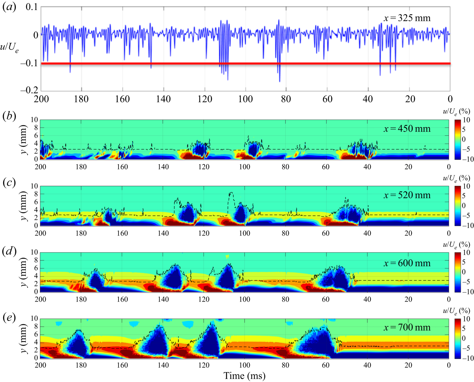
Figure 7(a) shows the velocity time series from a hot-wire probe immediately above the disturbance source (x = 325 mm) at y = 0.5 mm, while figures 7(b), 7(c), 7(d) and 7(e) show the ensemble-averaged streamwise fluctuating velocity contours at x = 450, 520, 600 and 700 mm, respectively, where the dotted lines indicate the boundary-layer thickness. Here, the mean velocity was obtained by time averaging the entire 400 ms long signal. It has been shown (Wang et al. Reference Wang, Choi, Gaster, Atkin, Borodulin and Kachanov2021) that only disturbances greater than 10 % of the free-stream velocity, as indicated by a red horizontal bar in the figure, developed to the turbulent spots downstream. For example, strong disturbances at t = 26, 30 and 36 ms developed to three incipient turbulent spots, as shown in figure 7(b), which merged to form a single turbulent spot later (see figure 7e). The weak disturbance at t = 62 ms decayed downstream after developing an incipient turbulent spot (see figure 7b). It should be noted that this threshold value depends on the wall-normal position of velocity measurement.
The velocity time series from a hot-wire probe immediately above the disturbance source (x = 325 mm) at y = 0.5 mm, z = 0 mm (a); the downstream development of the ensemble-averaged streamwise fluctuating velocity at (b) x = 450 mm, (c) x = 520 mm, (d) x = 600 mm and (e) x = 700 mm, where the dotted lines indicate the boundary-layer thickness.
The detailed structure of turbulent spots which were artificially initiated from the disturbance source was previously investigated, and their streamwise development was shown at x = 350, 380 and 400 mm (see figure 14 in Wang et al. Reference Wang, Choi, Gaster, Atkin, Borodulin and Kachanov2021). These results demonstrated that the turbulent spots were comprised of a number of low-speed pillars which were anchored at the wall, stretching out to the edge of the boundary layer. These pillars represented the low-speed regions of the turbulent spots which were pumped up within each hairpin-like structure. The high-speed regions of the turbulent spots were also observed near the wall in between the low-speed pillars. It was also shown that the number of hairpin-like structures increased in both streamwise and spanwise directions during their development until they merged together downstream.
Figure 8(a,b) shows the ensemble-averaged fluctuating streamwise velocities in the centre plane of the boundary layer at x = 520 mm (20 mm downstream of the control slot) without and with opposition control, respectively, where the dotted lines indicate the boundary-layer thickness. They clearly demonstrate that the high-speed region of the turbulent spots near the wall surface (shown in red in figure 8a) was cancelled by the wall-normal jet during control. The velocity of the boundary layer in between the turbulent spots was increased, however, as the boundary layer was drawn towards the wall during the suction phase of the audio speaker (see figure 5b). Figure 8(c) shows the velocity increment due to opposition control, indicating that the high-speed region of the turbulent spots was displaced by the low-speed fluid of the wall-normal jet. The velocity time series in the boundary layer with opposition control at different wall-normal positions are shown in figure 8(d), indicating that the entire boundary layer was affected by opposition control.
Effect of opposition control on the turbulent spots at x = 520 mm, z = 0 mm. (a) Ensemble-averaged fluctuating velocity contour without control and (b) with control, where the dotted lines indicate the boundary-layer thickness; (c) change in the streamwise velocity due to opposition control; (d) the velocity time series with control at y = 0.5, 1, 2 3 and 4 mm.
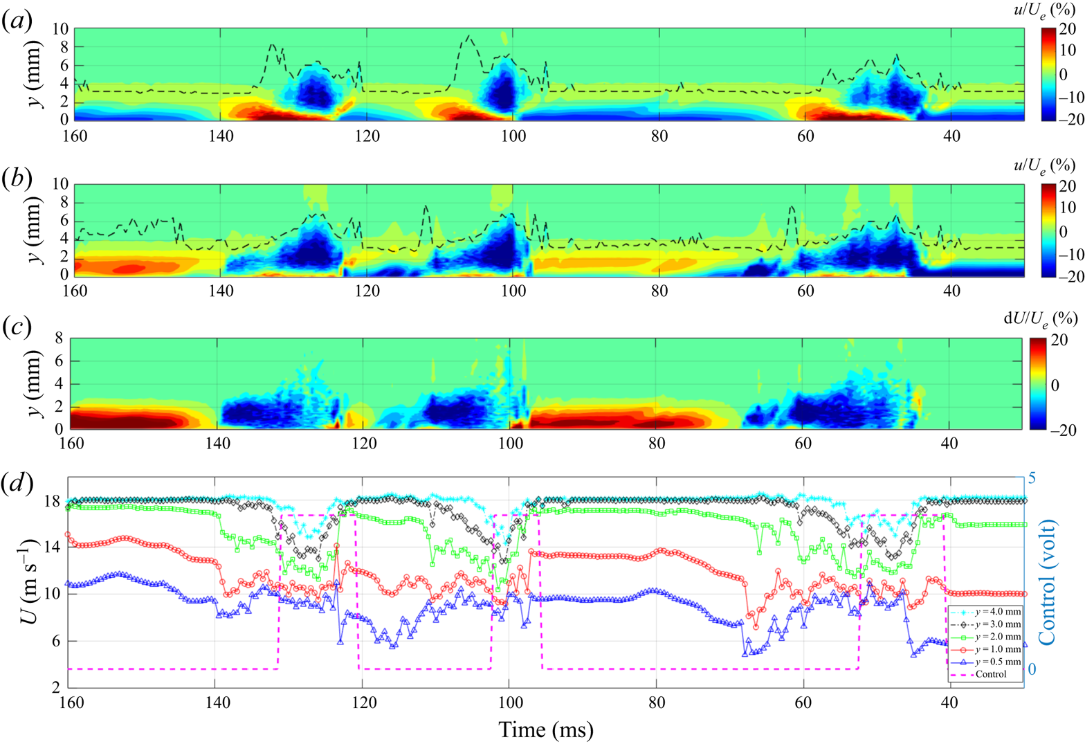
Figure 9(a,b) shows the ensemble-averaged streamwise velocities in the centre plane of the boundary layer at x = 600 mm without and with opposition control, respectively, showing the lasting effect of opposition control of the turbulent spots 100 mm downstream of the control slot. The reduction of the high-speed region of the turbulent spots, as shown in red in figure 9(a), is still clear in figure 9(b), but the effectiveness of opposition control of turbulent spots seems to be reduced at this downstream location. The difference in the streamwise velocity without and with control is given in figure 9(c), which shows that the low-momentum fluid injected from the control slot at x = 500 mm is convected away from the wall, reducing the effectiveness of opposition control.
Effect of opposition control on the turbulent spots at x = 600 mm, z = 0 mm. (a) Ensemble-averaged fluctuating velocity contour without control and (b) with control, where the dotted lines indicate the boundary-layer thickness; (c) change in the streamwise velocity due to opposition control.

Figure 10 shows the effect of opposition control of turbulent spots, by comparing streamwise velocity time series in the boundary layer without (in blue) and with control (in red) at x = 520 mm (20 mm downstream of the control slot). Ensemble-averaged streamwise velocity fluctuations are shown in thick lines, while individual velocity time series in one of 20 repeated measurements are indicated by thin lines. At y = 0.5 and 1.0 mm (figures 10a and 10b, respectively) streamwise velocities within the turbulent spots were increased due to the downwash of high-momentum fluid (see figure 8a), which were selectively cancelled by the low-momentum fluid brought by the wall-normal jet during control. At y = 1.5, 2.0 and 3.0 mm (panels c, d and e, respectively), streamwise velocities within the turbulent spots were reduced as the low-speed pillars of hairpin-like structure stretch out to the boundary-layer edge (Wang et al. Reference Wang, Choi, Gaster, Atkin, Borodulin and Kachanov2021). Here, opposition control was able to prolong the duration of the velocity reduction at the trailing edge (upstream end) of the turbulent spot.
Effect of opposition control of the turbulent spots without control (in blue) and with control (in red) at the wall-normal position y = 0.5 mm (a), 1.0 mm (b), 1.5 mm (c), 2.0 mm (d) and 3.0 mm (e) at x = 520 mm, z = 0 mm. Ensemble-averaged and individual velocity time series are shown in thick lines and thin lines, respectively.

Boundary-layer profiles within a turbulent spot between t = 40 and 65 ms in the centre plane at x = 520 mm (the far-right spot in figures 7, 8 and 9) are shown in figure 11(a) without control (in blue) and with control (in red), demonstrating that the mean velocity of a turbulent spot was reduced by opposition control across the entire boundary-layer thickness. The profiles of root-mean-square (RMS) velocity fluctuation are shown in figure 11(b), indicating that the velocity fluctuation of a turbulent spot was reduced by opposition control close to the wall (y < 2 mm). The RMS velocity fluctuation away from the wall (y > 2 mm) was slightly increased by opposition control, however. Also, figure 11(c) shows the ensemble-averaged velocity profiles of a turbulent spot at t = 53 ms, which correspond to the centre (in time) of the high-speed region of the turbulent spot, where even a greater velocity reduction than that over the entire turbulent spot was obtained by opposition control (see figure 11a).
Response of the boundary layer to opposition control of a turbulent spot at x = 520 mm, z = 0 mm. Mean velocity profiles (a), profiles of RMS velocity fluctuation (b) and ensemble-averaged velocity profiles (c), without control (in blue) and with control (in red). The Blasius profiles are shown by the dotted lines in (a) and (c).

The same set of velocity profiles at x = 660 mm are given in figure 12, showing the persistence of opposition control of a turbulent spot further downstream. Here, the effect of wall-normal jet is seen near the edge of the boundary layer, see figure 12(a). In other words, the low-momentum fluid of the wall-normal jet moved across the boundary layer at this downstream location. This is clearly seen in figure 12(a) for the mean velocity profiles over the entire turbulent spot, as well as in figure 12(c) for the ensemble-average velocity profiles of at the centre of the high-speed region of the turbulent spot. A reduction of the RMS velocity fluctuation by control is still observed at x = 660 mm in the range 0 mm < y < 3 mm, as shown in figure 12(b), although there is an increase in RMS velocity fluctuation at y > 4 mm.
Response of the boundary layer to opposition control of a turbulent spot at x = 660 mm, z = 0 mm. Mean velocity profiles (a), profiles of RMS velocity fluctuation (b) and ensemble-averaged velocity profiles (c), without control (in blue) and with control (in red). The Blasius profiles are shown by the dotted lines in (a) and (c).

In order to quantify the effectiveness of opposition control, the total turbulence energy in a turbulent spot is shown in figure 13 as a function of the downstream distance without and with control. Here, the total turbulence energy in a turbulent spot was obtained by integrating the turbulent kinetic energy u 2 across the entire boundary-layer thickness, which was divided by  $U_e^2\delta$ for non-dimensionalisation. Here, Ue is the free-stream velocity and δ is the boundary-layer thickness. Figure 13 demonstrates that the total turbulence energy in a turbulent spot is reduced by 20 % to 30 % by opposition control, which lasted at least until x = 600 mm. The reduction in the total turbulence energy dropped to 7 % at x = 660 mm, indicating that the persistence of control is about 40 laminar boundary-layer thicknesses (or 20 turbulent boundary thicknesses in the turbulent spots). Figure 13 does not contain any contribution of turbulence energy from the control jet since the effect of wall-normal velocity component on the hot-wire probe is negligible 20 mm downstream of the control slot at x = 520 mm.
Streamwise development of the total turbulence energy of the boundary layer without control (in black) and with control (in red).

The displacement thickness δ* and the momentum thickness θ of the boundary layer are obtained at various times using the ensemble-averaged velocity profiles, and are given in figure 14 without control (in blue) and with control (in red) over the time period from t = 30 to 160 ms. The shape factor H, which is the ratio of the displacement thickness δ* and the momentum thickness θ, is also given in the same figure. Large increases in δ* and θ within the turbulent spots are clearly visible in the figure, indicating an increase in the boundary-layer thickness associated with transition of the laminar boundary layer to turbulence. Here, the relative increase in the momentum thickness within the turbulent spots was much greater than that of the displacement thickness, therefore the shape factor H was reduced within the turbulent spots (Wang et al. Reference Wang, Choi, Gaster, Atkin, Borodulin and Kachanov2021). Figure 14 shows that there is an increase in the displacement thickness δ* by opposition control, which was much greater than that of the momentum thickness θ, resulting in an increase in the shape factor H. No increase in the momentum thickness was observed either before or after control. However, the displacement thickness δ* was reduced outside the turbulent spots, reducing the shape factor H. This is due to the suction effect of the audio speaker towards the end of opposition control, which increased the velocity in the near-wall region by drawing the boundary layer towards the wall (see figure 5b). Here, the suction effect is an artefact of control during experiment, which must be minimised to improve the effectiveness of opposition control.
Integral parameter of the boundary layers and the shape factor based on the ensemble-averaged instantaneous velocity profiles measured without control (in blue) and with control (in red) at x = 520 mm, z = 0 mm.

In this study, an audio speaker with a flat circular cone operated in a pistonic mode was used as an actuator for opposition control, which is effectively a zero-net-mass-flux jet actuator. Here, the effect of added mass and momentum on the boundary-layer development in each control-on period can be evaluated by taking the average velocity and momentum of the wall-normal jet flow during control. This gives an increase of 2.2 % and 0.13 % in the displacement thickness δ* and the momentum thickness θ, respectively, which are negligible since they are within the measurement uncertainties. Therefore, any changes which can be observed in figure 14 are due to the modification of the boundary-layer structure by opposition control, but not due to the added mass or momentum by the actuator.
4.2. Spanwise structure of the turbulent spots
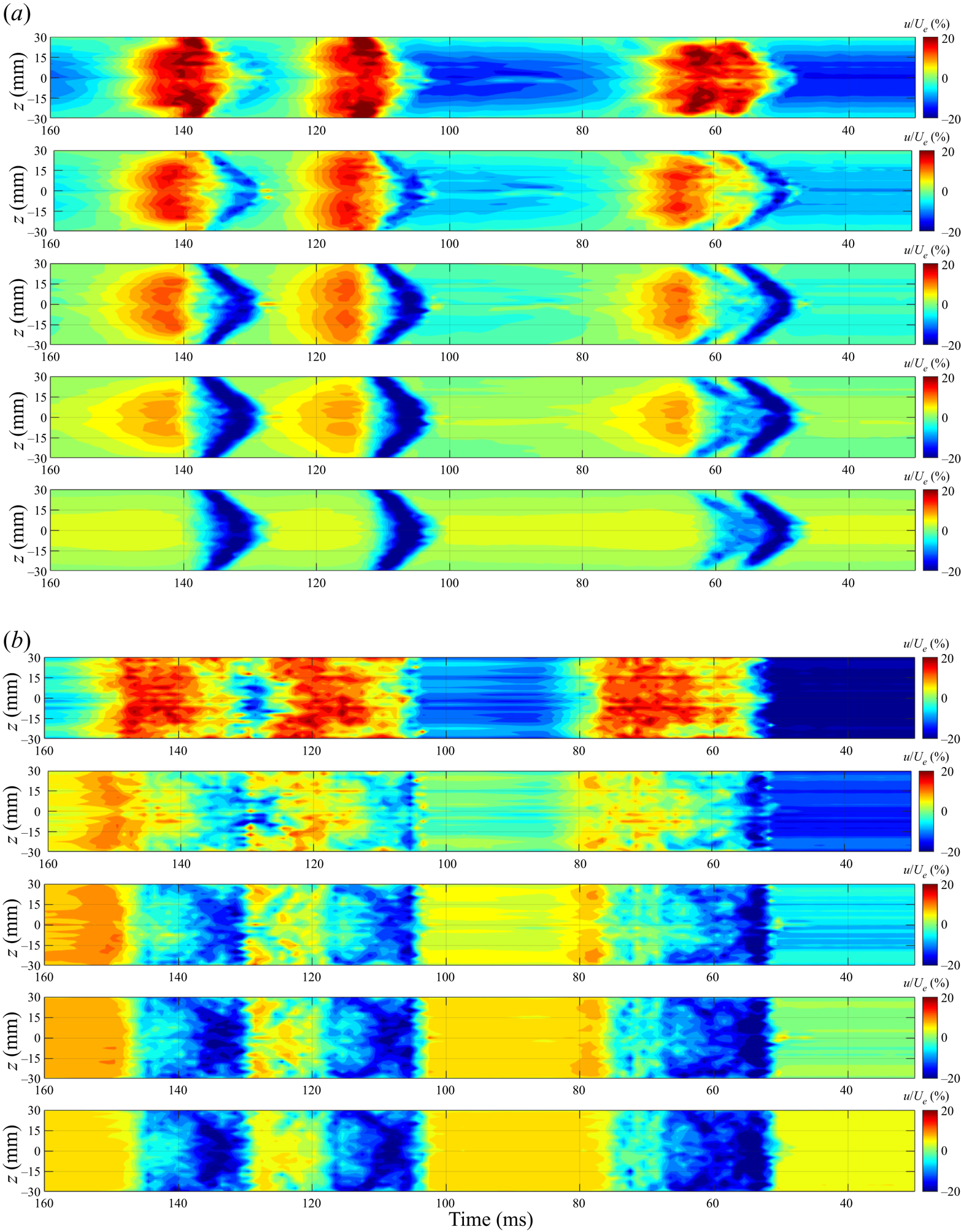
Figure 15(a,b) shows the spanwise structure of the turbulent spots in a plan view (t–z plane) without and with control, respectively, 20 mm downstream of the control slot (x = 520 mm), where the streamwise velocity fluctuations are displayed at y = 0.5, 1.0, 1.5, 2.0 and 3.0 mm from top to bottom of each panel. Similarly to all previous figures, the time sequence is reversed here, so that the turbulent spots’ orientation corresponds to physical space in the x–y plane. It is clear that opposition control eliminated the high-speed region of the turbulent spots in the entire spanwise range from z = −30 to 30 mm, see figure 15(a), by replacing them with a carpet of low-speed region as shown in figure 15(b). Within the low-speed carpet created by opposition control, the silhouette of turbulent spots still remains, however. Since the low-speed fluid was also used to stop the downwash of the high-speed fluid, the opposition control strategy used in this study should be considered as a combination of out-of-phase v-velocity control with in-phase u-velocity control (Choi et al. Reference Choi, Moin and Kim1994), where v and u are wall-normal and streamwise velocities, respectively. In other words, opposition control was carried out not only to stop the downwash of high-momentum fluid, but also to reduce the streamwise fluid momentum. A similar technique was used by Rebbeck & Choi (Reference Rebbeck and Choi2001, Reference Rebbeck and Choi2006) in their wind tunnel demonstration of opposition control of the sweep events in the turbulent boundary layer. It should be noted that the velocity increase in the boundary layer in between the turbulent spots was due to the suction phase of the audio speaker following the injection of low-speed fluid by the wall-normal jet. The apparent spanwise spread of the turbulent spots as a result of opposition control, as seen in figure 15(b), is due to the 64 mm long control slot for wall-normal jets, whose length was chosen to cover the entire spanwise high-speed region of the turbulent spots.
Downstream development of the ensemble-averaged streamwise fluctuating velocity in the spanwise planes at y = 0.5, 1.0, 1.5, 2.0 and 3.0 mm, from top to bottom at x = 520 mm, without control (a) and with opposition control (b).
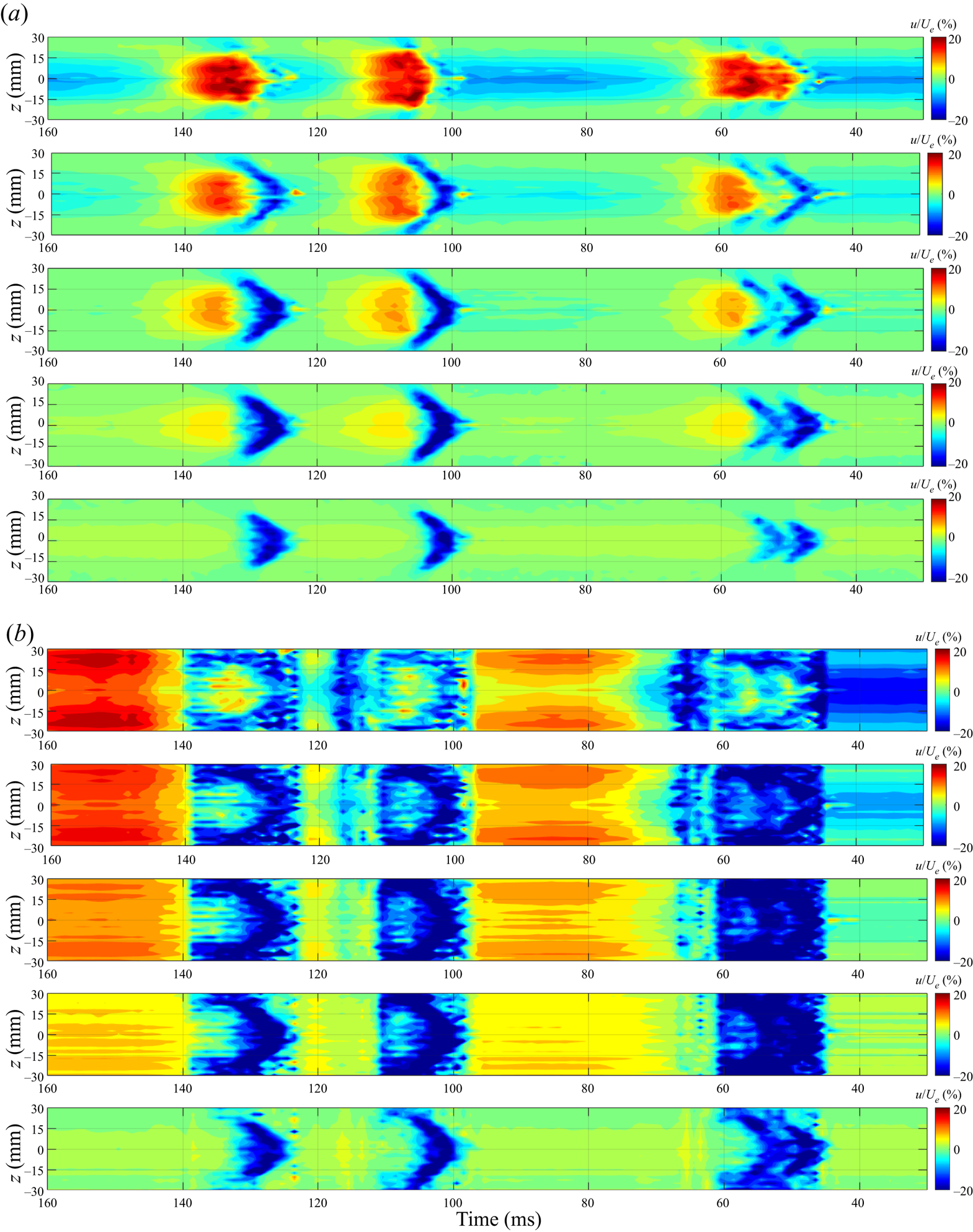
The downstream development of the turbulent spots is shown in figures 16(a) and 16(b) without and with control, respectively, 100 mm downstream of the control slot (x = 600 mm). Again, streamwise velocity fluctuations at y = 0.5, 1.0, 1.5, 2.0 and 3.0 mm are displayed from top to bottom of each figure, showing the modification to the spanwise structure of the turbulent spots at this downstream location. Figure 16(b) demonstrates that opposition control was still effective 100 mm downstream of the control slot, showing that the high-speed region of the turbulent spots was cancelled by the low-speed fluid brought by the wall-normal jet in almost the entire spanwise range of the turbulent spot. However, the low-momentum fluid injected from the control slot at x = 500 mm was convected away from the wall (see in figure 6c) at x = 600 mm, resulting in an emergence of a thin high-speed region close to the wall.
Downstream development of the ensemble-averaged streamwise fluctuating velocity in the spanwise planes at y = 0.5, 1.0, 1.5, 2.0 and 3.0 mm, from top to bottom at x = 600 mm, without control (a) and with opposition control (b).
Perspective views of turbulent spots without and with opposition control are given in figures 17(a) and 17(b), respectively, 20 mm downstream of the control slot (x = 520 mm). Here, iso-surfaces of ensemble-averaged streamwise velocity fluctuations at 15 % (orange) and −15 % (blue) are shown These figures confirm the results given in figures 15(a) and 15(b), demonstrating that the high-speed region near the trailing edge (upstream end) of the turbulent spots, as shown in orange in the figure, was destroyed by opposition control using wall-normal jets. However, the wing-shaped, low-speed region near the leading edge (downstream end) of the turbulent spots, as shown in blue, is still visible after opposition control. Figure 18(a) shows the perspective view of turbulent spots which were grown in size at x = 600 mm, yet the effectiveness of opposition control in cancelling the high-speed region is still evident.
Perspective views of turbulent spots without (a) and with control (b) at x = 520 mm, which are depicted by iso-surfaces of ensemble-averaged streamwise velocity fluctuations at 15 % (orange) and −15 % (blue) of the free-stream velocity.

Perspective views of turbulent spots without (a) and with control (b) at x = 600 mm, which are depicted by iso-surfaces of ensemble-averaged streamwise velocity fluctuations at 15 % (orange) and −15 % (blue) of the free-stream velocity.

Spanwise modulation of the wall-normal profiles of instantaneous streamwise velocity measured within a turbulent spot (the second spot from the right in figures 7, 8 and 9) at various times from t = 95 to 120 ms at x = 520 mm is shown in figures 19 and 20 without control and with control, respectively. Here, only the positive spanwise side of the velocity profiles are displayed to avoid repetitions. The wall position of the modulated velocity profiles was determined by extrapolating the measured Blasius velocity profile without excitation to the origin (as shown by the dotted line). It should be noted that the turbulent spot shown in figures 19 and 20 is different from that in figures 11 and 12. Without control there is an increase in the boundary-layer thickness along the centreline (z = 0 mm) at the leading edge (downstream end) of the turbulent spot (t = 101 ms), which was quickly reduced back to the original thickness towards the trailing edge at t = 110 ms when the high-speed region started to appear in the turbulent spot (see figure 19b). The velocity deficit in the boundary-layer profile associated with the increase in the boundary-layer thickness is also seen in figures 19(c) and 19(d) at z = 5 and 10 mm, respectively. At z = 15 mm (see figure 19e), the velocity profile remained unchanged from t = 95 to 120 ms, indicating that the half-width of this turbulent spot is approximately 20 mm.
Ensemble-averaged streamwise velocity distribution in a spanwise plane (y = 1 mm) at x = 520 mm without control (a), and the spanwise modulation of the wall-normal profiles of instantaneous velocity measured within a turbulent spot from t = 95 to 120 ms at z = 0 mm (b), z = 5 mm (c), z = 10 mm (d), z = 15 mm (e) and at z = 20 mm ( f).

Ensemble-averaged streamwise velocity distribution in a spanwise plane (y = 1 mm) at x = 520 mm with control (a), and the spanwise modulation of the wall-normal profiles of instantaneous velocity measured within a turbulent spot from t = 95 to 120 ms at z = 0 mm (b), z = 5 mm (c), z = 10 mm (d), z = 15 mm (e) and at z = 20 mm ( f).

Spanwise modulation of the wall-normal profiles of instantaneous streamwise velocity measured within a turbulent spot at various times (from t = 95 to 120 ms) with opposition control is shown in figure 20, indicating that the boundary-layer thickness of the turbulent spot was not significantly affected by control along the centreline (z = 0 mm), see figure 20(b). However, the velocity deficit in the velocity profile was greatly increase by control between t = 101 and 110 ms. Figure 20(d–f) shows that the low-momentum fluid of the wall-normal jet has modified the off-centre structure of the turbulent spot beyond z = 10 mm, by increasing the velocity deficit further between t = 101 and 110 ms. Note that the wall-ward shift of the velocity profile at t = 97 ms was due to the suction phase of an audio speaker following the injection of low-speed fluid during opposition control of turbulent spot between t = 40 and 70 ms.
4.3. Turbulence structure within the turbulent spots
It was shown by Wang et al. (Reference Wang, Choi, Gaster, Atkin, Borodulin and Kachanov2021) that the turbulent spots consist of hairpin-like low-speed pillars that are anchored at the wall, which stretch out to the edge of the boundary layer pumping up low-speed fluid. The high-speed region of the turbulent spot was found near the wall as a result of downwash of high-momentum fluid in between the low-speed pillars (Schroder & Kompenhans Reference Schroder and Kompenhans2004). A strong similarity in the turbulence structure between the turbulent spots and fully developed turbulent boundary layers was indicated by Wygnanski et al. (Reference Wygnanski, Sokolov and Friedman1976), Johansson et al. (Reference Johansson, Her and Haritonidis1987) and Wu et al. (Reference Wu, Moin, Wallace, Skarda, Lozano-Durán and Hickey2017). Here, we used the VITA technique (Blackwelder & Kaplan Reference Blackwelder and Kaplan1976) to investigate the effect of opposition control on the near-wall turbulence within the high-speed region of the turbulent spots. The VITA technique examines the running-averaged standard deviation of the fluctuating velocity in order to extract signals that are associated with the near-wall turbulence events such as sweeps and ejections. Since the u- and v-velocities are strongly correlated to each other during these turbulence events, which account for nearly all of the turbulence production in the near-wall region (Kim, Kline & Reynolds Reference Kim, Kline and Reynolds1971). As such, only the u-component velocity can be used to successfully detect the sweep or ejection events. The running-average time must be equal to the characteristic time scale of the turbulence events in the near-wall region, which was set to t+ = tu* 2/ν = 13.5 (t = 0.3 ms) in the present study. The friction velocity u* = 0.82 m s−1 was estimated using a power-law correlation between the skin-friction coefficient Cf and the momentum thickness θ of the boundary layer,  ${C_f} = 0.024Re_\theta ^{ - 1/4}$ (Smits, Matheson & Joubert Reference Smits, Matheson and Joubert1983). This gave the ratio of the free-stream velocity to the friction velocity of Ue/u* = 22 at the Reynolds number of Reθ = 1080. Here, the momentum thickness of the boundary layer within the turbulent spots was θ = 0.9 mm at x = 520 mm (see figure 9) and the kinematic viscosity of air was ν = 1.5 × 10⁻⁵ m2 s−1. In order to reduce the effect of undulating velocity within the turbulent spots (see figure 7), each velocity signal was subtracting by the ensemble-averaged velocity before applying the VITA technique. The threshold value for the VITA detection was set to 0.75σu, where σu is the standard deviation of each velocity signal, either without control or with control. It was shown by Blackwelder & Kaplan (Reference Blackwelder and Kaplan1976) that the threshold value of the VITA detection does not influence the conditionally sampled velocity signatures as they collapse into a single curve when normalised by the threshold value. Only the rising velocity signal corresponding to the sweep events was detected, rejecting all falling signals for ejection events. The window width was set to T+ = 67.5 (T = 1.5 ms).
Figure 21 shows the VITA-detected burst signatures during the sweep events within the high-speed regions of the turbulent spots without (in black) and with opposition control (in red) at x = 520 mm. They are ensemble-averaged and normalised by the maximum velocity variation for comparison at y = 0.3 mm (y+ = 16), 0.5 mm (y+ = 27) and 1.0 mm (y+ = 55). It is clear from these results that the duration of the burst signatures in the high-speed region was reduced by opposition control of the turbulent spots. A similar reduction in the duration of the burst signature has been observed in many drag-reducing flows. For example, riblets reduce the skin-friction drag of the turbulent boundary layer by up to 8 % (Walsh & Lindemann Reference Walsh and Lindemann1984), where nearly 50 % reduction in the duration of the burst signature was observed (Bacher & Smith Reference Bacher and Smith1985; Choi Reference Choi1989). The duration of the burst signature within the viscous sublayer of the turbulent boundary layer with spanwise-wall oscillation, which gives more than 40 % of turbulent drag reduction (Jung, Mangiavacchi & Akhavan Reference Jung, Mangiavacchi and Akhavan1992; Choi, DeBisschop & Clayton Reference Choi, DeBisschop and Clayton1998), was only one third of that without wall oscillation (Choi & Clayton Reference Choi and Clayton2001). Even in the buffer region of the turbulent boundary layer, the effect of wall oscillation on the burst signature was still significant, with its duration nearly a half of that without wall oscillation.
VITA-detected burst events at  $x = 520$ mm, $y = 0.3$ mm and $z = 0$ mm, where the ensemble averaged signatures are shown in a thick line without control (a) and with control (b). Ensemble averaged burst signatures are also compared at $y = 0.3$ mm (c), $y = 0.5$ mm (d) and $y = 1.0$ mm (e) without (in black) and with opposition control (in red). The threshold value was set to 0.75 $\sigma_u$, where $\sigma_u$ is the standard deviation of each velocity signal.

The frequency of burst events was increased by opposition control, which became more significant with an increase in the threshold value of VITA detection. Figure 22 shows the number of VITA-detected burst events over 8 s of measurements without (in blue) and with control (in red) at a function of the threshold value at x = 520 mm at y = 0.3 mm (y+ = 16), y = 0.5 mm (y+ = 27) and y = 1.0 mm (y+ = 55). The percentage increase due to opposition control is also shown in black dotted line. As expected, the number of burst detections was reduced with an increase in the threshold value. It is clearly shown in figure 22, however, that the number of bursts was increased with opposition control for a given threshold value. For example, nearly 200 % increase in the burst frequency was detected with the threshold value of 0.75σu at y = 0.3 mm (y+ = 16) and y = 0.5 mm (y+ = 27). In comparison, it was shown that the frequency of the burst events detected over drag-reducing riblets was nearly eight times that over the smooth surface (Choi Reference Choi1989). This increase in the number of the burst events by opposition control is a reflection of an increase in the positive-tail probability as shown in figure 23, where probability densities of streamwise velocity fluctuations within the turbulent spot between t = 40 and 65 ms are shown without control (in black) and with control (in red). It should be noted that the RMS velocity fluctuations within the turbulent spots were reduced by up to 50 % at y < 1.5 mm (see figure 8b) by opposition control. Therefore, opposition control modified the near-wall turbulence structure in such a way that the burst events became weaker and shorter but more frequent.
The number of VITA-detected burst events over 8 s of measurements without (in blue) and with control (in red) as a function of the threshold value relative to the standard deviation σu of each velocity signal at x = 520 mm, z = 0 mm. Percentage increase in the number of VITA-detected burst events due to opposition control is also shown at y = 0.3 mm (a), y = 0.5 mm (b) and y = 1.0 mm (c).

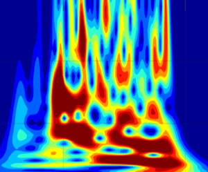
The effect of opposition control on the turbulence energy distribution within the turbulent spots was investigated using generalised Morse wavelets (Lilly & Olhede Reference Lilly and Olhede2012), where the symmetry parameter and the time-bandwidth product were set to γ = 3 and P 2 = 60, respectively (Wang et al. Reference Wang, Choi, Gaster, Atkin, Borodulin and Kachanov2021). Figures 24(a) and 25(a) show the individual velocity signals (in red) and the ensemble-averaged velocity signals (in black) of three turbulent spots between t = 30 and 160 ms at x = 520 mm and y = 1.0 mm without control and with control, respectively. The reduction in the turbulence intensity by opposition control was nearly maximum at this wall-normal location, see figure 8(b). Figures 24(b) and 25(b) are the ensemble-averaged wavelet spectra of 20 repeated velocity measurements (not the wavelet spectra of ensemble-averaged velocity signals) at the same wall-normal locations without control and with control, respectively. The individual wavelet spectra are shown in figures 24(c) and 25(c) without control and with control, respectively. The spectral increment due to control is shown in figures 26(b) and 26(c) for the ensemble-averaged wavelet spectrum and the individual wavelet spectrum, respectively, after subtracting the wavelet spectra without control (figure 24b,c) from those with control (figure 25b,c). Here, the spectral increments at the trailing edge (upstream end) of the turbulent spots (at t = 60, 110 and 140 s) are due to the longer control duration than necessary for opposition control (see figure 26a for a comparison of velocity fluctuations between the baseline and the control case). Figures 26(b) and 26(c) indicate a reduction in the turbulence energy within the turbulent spots due to control between f = 0.5 and 2.0 kHz, which correspond to a typical burst frequency as shown in figure 21. Figure 26(c) also shows an increase in the high-frequency turbulence energy above f = 2.0 kHz, which is related to the increase in the positive-tail probability by opposition control (see figure 23).
Probability densities (PDF) of streamwise velocity fluctuation within the turbulent spot between t = 40 and 65 ms at x = 520 mm, z = 0 mm at y = 0.3 mm (a), y = 0.5 mm (b) and y = 1.0 mm (c) without control (in black) and with control (in red).

Individual velocity signal (in red) and the ensemble-averaged velocity signal (in black) of turbulent spots (a), ensemble-averaged wavelet spectrum of 20 repeated velocity measurements (b) and the individual wavelet spectrum (c) in the boundary layer at x = 520 mm, y = 1.0 mm and z = 0 mm without control.

Individual velocity signal (in red) and the ensemble-averaged velocity signal (in black) of turbulent spots (a), ensemble-averaged wavelet spectrum of 20 repeated velocity measurements (b) and the individual wavelet spectrum (c) in the boundary layer at x = 520 mm, y = 1.0 mm and z = 0 mm with control.

Individual velocity signals (thin line) and the ensemble-averaged velocity signals (thick line) of turbulent spots without control (in black) and with control (in red) (a), the spectral increment in the ensemble-averaged wavelet spectrum by control (b) and the spectral increment in the individual wavelet spectrum by control (c) in the boundary layer at x = 520 mm, y = 1.0 mm and z = 0 mm.

5. Concluding remarks
Opposition control of artificially initiated turbulent spots in a laminar boundary layer over a flat plate was carried out in a low-turbulence wind tunnel. The aim of this study was to delay the process of transition to turbulence by modifying the near-wall turbulence structure of the turbulent spots. Opposition control was carried out not only to stop the downwash of high-momentum fluid, but also to reduce the streamwise fluid momentum, where the timing and duration of opposition control were pre-determined based on the baseline measurements of the turbulent spots. In other words, the opposition control strategy employed in this study was a combination of out-of-phase v-velocity control with in-phase u-velocity control (Choi et al. Reference Choi, Moin and Kim1994; Rebbeck & Choi Reference Rebbeck and Choi2001, Reference Rebbeck and Choi2006). Our experimental results clearly showed that the high-speed fluid of the turbulent spots near the wall was replaced by the low-speed fluid of the wall-normal jet.
Opposition control reduced the mean velocity in the turbulent spot across the entire boundary layer. The reduction in the velocity was greatest at the centre of the high-speed region of the turbulent spot where opposition control was performed. It was also observed that the RMS velocity fluctuations were reduced by opposition control close to the wall. Between 20 % and 30 % of the total turbulence energy in the turbulent spots was reduced by wall-normal jets during opposition control, although the reduction became smaller further downstream. These results suggest that the persistence of control is approximately 40 laminar boundary-layer thicknesses (or 20 turbulent boundary thicknesses in the turbulent spot).
The increase in the displacement thickness δ* by opposition control was greater than that of the momentum thickness θ, resulting in an increase in the shape factor H. No increase in the momentum thickness was observed either before or after control. However, the displacement thickness δ* was reduced outside the turbulent spots, reducing the shape factor H at the same time. This was due to the suction effect of the audio speaker used for control, which increased the velocity by drawing the boundary layer towards the wall at the end of opposition control.
The sweep events within the high-speed regions of the turbulent spots were studied using the VITA technique, where a reduction in the duration of the burst signatures was shown with opposition control. A similar reduction in the duration of the burst signature was observed in the turbulent boundary layer over riblets (Bacher & Smith Reference Bacher and Smith1985; Choi Reference Choi1989) and with spanwise-wall oscillation (Choi & Clayton Reference Choi and Clayton2001) as a result of turbulent skin-friction reduction. The burst frequency was increased with opposition control, which became more significant with an increase in the threshold value of the VITA detection.
The effect of opposition control on the turbulence energy distribution within the turbulent spots was investigated using generalised Morse wavelets. The ensemble-averaged wavelet spectra indicated that the turbulence energy within the turbulent spots corresponding to the typical burst frequency was reduced by opposition control. The wavelet spectra also showed an increase in the high-frequency turbulence energy relating to the increase in the positive-tail probability with control.
The effectiveness of opposition control in cancelling the high-speed region of the turbulent spots was demonstrated in this study. However, the control duration was slightly longer than was necessary at the trailing edge near the calmed region of the turbulent spots. The suction phase of the speaker diaphragm also adversely affected the control effectiveness, increasing the velocity in between the turbulent spots. These problems can be resolved by optimising the control parameters of the actuator. The issues of the limited persistence of opposition control can be tacked by adding booster control slots downstream after the initial control effect waned. A definitive confirmation of transition delay by opposition control is desirable, where a direct measurement of the skin-friction drag of the boundary layer may help together with improvements suggested above.
Funding
This work was supported by EPSRC grant EP/M028690/1.
Declaration of interests
The authors report no conflict of interest.


 Open access