





1. Introduction
1.1. The broader context
Numerical modelling of ocean gravity waves is a challenging task that has been studied extensively for more than two centuries. Ocean waves exhibit complex behaviours due to their nonlinear nature, particularly under steep-wave conditions. Understanding and predicting ocean wave dynamics are vital for various applications, including coastal engineering, obtaining loads for structural integrity assessment and environmental impact assessment, to name a few. On large (global) scales, phase-averaged models such as WaveWatch 3 (see Tolman Reference Tolman1991) or SWAN (Booij, Holthuijsen & Ris Reference Booij, Holthuijsen and Ris1996) have been used with great success in the last few decades to estimate the propagation of wave energy across the upper ocean, in the open ocean and near shore. These semi-empirical, third-generation phase-averaged models are today the backbone of most meteorological wave prediction models, providing wave predictions (forecast) and historical reanalysis of wave conditions (hindcast) (see Sterl, Komen & Cotton Reference Sterl, Komen and Cotton1998; Saha et al. Reference Saha2010; Hersbach et al. Reference Hersbach2020). The latter provides input for the site-specific assessment of the long-term environment, which is essential knowledge in the design of offshore and coastal engineering. However, the datasets are limited to phase-averaged statistical properties of sea states, not sufficient to describe the individual wave properties, such as the complex wave kinematics of individual waves, needed for wave load assessment. For this, phase-resolved wave models are needed.
There are several phase-resolved wave models and wave theories that are commonly used to describe the evolution of individual waves. However, the models have varying capabilities when it comes to modelling the different physical processes of gravity waves.
In deep or intermediate water depths, well-established wave theories for irregular waves, such as linear or second-order wave theory (Sharma & Dean Reference Sharma and Dean1981; Smit, Janssen & Herbers 2017), are frequently used in engineering and design, to obtain wave kinematics for load assessment. However, it is well known that especially linear wave theory is not very representative of steeper waves, and second-order wave theory is limited to weakly nonlinear waves.
In shallow waters, wave equations with mild-slope assumptions have been effectively adopted for studying coastal wave propagation, but they do not hold up well for sites with significant depth changes.
Boussinesq-type models (Madsen, Murray & Sørensen Reference Madsen, Murray and Sørensen1991; Madsen & Sørensen Reference Madsen and Sørensen1992; Nwogu 1993) offer efficient alternatives, but historically struggle with strong dispersion in deep waters. Although significant effort and progress have been made to enhance the dispersive abilities of Boussinesq-type models over the years (see e.g. Wei et al. (Reference Wei, Kirby, Grilli and Subramanya1995) or the FUNWAVE model (Kirby et al. Reference Kirby, Wei, Chen, Kennedy and Dalrymple1998)), the high order of derivatives is a challenge for numerical stability.
Lynett & Liu (Reference Lynett and Liu2004) took a different approach and divided the vertical water column into layers using polynomials that were matched at the interfaces. This multi-layer approach showed excellent performance on linear dispersive properties compared with the single-layer Boussinesq models, even with few layers. Although the cost of computation originally increased greatly with the additional layers, developments done in later years (see Zijlema, Stelling & Smit Reference Zijlema, Stelling and Smit2011; Popinet Reference Popinet2020) have shown that it is capable of modelling nearly all of the physical processes related to waves in variable water depth, albeit the layered grid structure prevents waves from overturning.
Another branch of wave models are the nonlinear potential flow solvers, for which there exist several approaches to solve the Laplace equation. These include boundary element methods (see Grilli et al. Reference Grilli, Losada and Martin1994, Reference Grilli, Horrillo and Guignard2020), higher-order spectral methods (see Dommermuth & Yue Reference Dommermuth and Yue1987; Ducrozet et al. Reference Ducrozet, Bonnefoy, Le Touzé and Ferrant2016) or volume-based methods such as those of Li & Fleming (Reference Li and Fleming1997), Bingham & Zhang (Reference Bingham and Zhang2007), Engsig-Karup, Bingham & Lindberg (Reference Engsig-Karup, Bingham and Lindberg2009) and Wang et al. (Reference Wang, Pákozdi, Kamath and Bihs2021) to mention a few.
Although many of the aforementioned models and theories are fundamental and frequently used, these models lack the capability to physically model breaking waves. As a result, many account for breaking by introducing empirical breaking onset models, such as described by Barthelemy et al. (Reference Barthelemy, Banner, Peirson, Fedele, Allis and Dias2018) and Derakhti, Banner & Kirby (Reference Derakhti, Banner and Kirby2018), to obtain more realistic wave evolution and energy dissipation and at the same time prevent numerical breakdown of the simulation as a result of plunging breakers.
However, being able to model an actual breaking wave is important. As waves break, the local increase in horizontal kinetic energy can lead to severe impact loads on a structure. As a testimony to this, we refer to an extensive list of reported wave-breaking related impact events, presented in van Essen & Seyffert (Reference van and Seyffert2023). The loads of such events may for many structures be a governing force for design (as discussed in Lian & Haver (Reference Lian and Haver2016) and Johannessen & Lande (Reference Johannessen and Lande2018)). Although breaking onset models may give statistically good agreement, they cannot be trusted with a good spatio-temporal description of the complex kinematics in breaking waves for load assessment. In a wave evolution perspective, breaking also leads to energy dissipation, which for a coastal site with complex bathymetry may be inaccurately estimated using empirical dissipation models, which are often based on idealised experimental conditions (see Tian, Perlin & Choi Reference Tian, Perlin and Choi2010; Craciunescu & Christou Reference Craciunescu and Christou2020).
An alternative is therefore to use wave models that model the actual breaking. Over the last two decades, computational fluid dynamics (CFD) wave models, based on Navier–Stokes or Euler equations, have attracted much attention because of their ability to model breaking waves. This includes the complex turbulent flow and air entrainment that follow breaking (Lubin & Glockner Reference Lubin and Glockner2015; Deike, Melville & Popinet Reference Deike, Melville and Popinet2016). However, two-phase flow Navier–Stokes models are not without challenges. The flow problem of wave propagation with high density ratios between air and water, combined with shear flow over the surface boundary, is numerically demanding (see Desjardins & Moureau Reference Desjardins and Moureau2010; Remmerswaal Reference Remmerswaal2023) and as such is not trivial. Common for all these models is that Navier–Stokes equations are solved iteratively by time-stepping the flow over a discretised domain (structured or unstructured grid). This makes them computationally expensive and may struggle with conservation of different properties of the flow over time, such as energy conservation (see Coppola et al. Reference Coppola, Capuano and de Luca2019, Buist et al. Reference Buist, Sanderse, Dubinkina, Henkes and Oosterlee2022).
Nevertheless, today a wide range of CFD solvers are available which may be used for propagation of surface gravity waves. However, different numerical schemes and methods are used, and their performance and accuracy may vary substantially. Therefore, the integrity and reliability of the use of these models rely on rigorous validation against experimental data. Validation not only ensures that the models reflect real-world physical behaviour with high fidelity, but also the user experience in choosing the right parameters and settings to obtain accurate results. Open-access experimental campaigns for validation assessment are therefore important and necessary, boosting confidence in wave models and their application for practical engineering and research problems. Ultimately, when used correctly, they offer a pathway to better predictions and insight into wave behaviour and wave-induced loading conditions, and thus may support the safe and efficient design of marine and coastal infrastructure.
In the scientific literature, a substantial number of laboratory investigations of irregular wave fields, including focused wave groups, have been reported. However, most classical datasets (e.g. Rapp & Melville Reference Rapp and Melville1990; Banner & Peirson Reference Banner and Peirson2007; Tian et al. Reference Tian, Perlin and Choi2010; Craciunescu & Christou Reference Craciunescu and Christou2020) were primarily developed to examine the fundamental physics of wave breaking and associated energy dissipation processes, rather than to provide deterministic validation cases for numerical models. As a result, these experiments frequently lack one or more essential components required for rigorous model benchmarking, such as well-defined and fully documented boundary conditions, reproducible wave-maker input signals, sufficiently long propagation distances, repeated realisations to enable uncertainty quantification, span over wave steepness/water depth and comprehensive measurements encompassing both free-surface elevation and subsurface velocity fields.
In the present study, we have designed and executed a model testing experiment aimed at producing a compact and consolidated dataset of accurately measured waves, intended for the validation of numerical wave models. The primary objective was not exploratory in a physical sense, but rather to develop a dataset spanning a broad range of conditions, specifically designed to discriminate effectively between the predictive capabilities of different phase-resolved wave models. To accomplish this, we established the following criteria for the experiment:
-
(i) Wave dispersion: Dispersive waves should be used to evaluate the dispersion capabilities of wave models.
-
(ii) Inhomogeneous conditions: The experimental set-up should encompass varying depths, transitioning from deep to shallow water, to assess the models’ capacity to propagate waves under inhomogeneous conditions.
-
(iii) Propagation length: Waves are required to propagate over several wavelengths, facilitating the evaluation of the models’ performance with respect to dispersive waves and energy conservation.
-
(iv) Wave input: The wave input conditions must be well defined and readily reproducible across most wave models.
-
(v) Wave steepness: The dataset should include the complete range of wave steepness, from linear low-amplitude waves to strong nonlinear and breaking waves.
-
(vi) Repeatability: All tests must be repeated several times, to ensure consistent and reliable output. The dataset should have sufficient resolution and adequate quality to make deterministic comparisons of the results.
-
(vii) Kinematics: Kinematics should be measured to make a comparison of velocities and momentum underneath the waves.
-
(viii) Duration: The validation dataset is designed to be compact, minimising the duration and number of tests required for validation, given that the most advanced phase-resolved wave models are computationally intensive.
Based on these criteria, we conducted an experiment using focused wave groups over different bathymetry, which should pose a challenge for most wave models to reproduce. As such, our first objective is to create a dataset that can help distinguish the performance of different wave models. We later demonstrate that the dataset is indeed reproducible by using a state-of-the-art CFD wave model.
This article is organised as follows. In the following section, we detail the experimental set-up, provide a justification for our design choices and evaluate the accuracy of the resulting dataset. Section 3 introduces a CFD wave model, which we propose is capable of deterministically reproducing the experimental dataset without necessitating extensive tuning of the numerical model or the boundary input. We validated the wave model against the experimental results by comparing surface elevations, wave kinematics and energetics. Finally, we present benchmarking results that can serve as a reference for validating other wave models using the provided dataset.
2. Laboratory experiments
Dispersive focused wave groups have been the subject of extensive investigation over the years. In the early 1990s, Rapp & Melville (Reference Rapp and Melville1990) conducted pioneering research on the energy dissipation of single breaking focused waves, laying the groundwork for numerous subsequent studies on breaking-wave energy dissipation, including those by Banner & Peirson (Reference Banner and Peirson2007), Drazen, Melville & Lenain (Reference Drazen, Melville and Lenain2008), Tian et al. (Reference Tian, Perlin and Choi2010) and Craciunescu & Christou (Reference Craciunescu and Christou2020).
Baldock, Swan & Taylor (Reference Baldock, Swan and Taylor1996) and Johannessen (Reference Johannessen1997) explored the nonlinear effects in non-breaking focused wave groups, making comparisons with second-order irregular wave theory and higher-order boundary element methods. In the context of coastal waters, Synolakis (Reference Synolakis1987) examined the run-up of solitary waves on a sloping beach, while Beji & Battjes (Reference Beji and Battjes1993) investigated the behaviour of regular wave trains over a submerged bar.
Recent studies have also focused on waves in coastal environments. Watanabe, Tsuda & Saruwatari (Reference Watanabe, Tsuda and Saruwatari2020) investigated wave focusing in shallow waters on both flat and sloping bottoms, while Whittaker et al. (Reference Whittaker, Fitzgerald, Raby, Taylor, Orszaghova and Borthwick2017) examined wave behaviour on a plane beach. While these studies represent significant advances in the field, most were not specifically designed to facilitate the re-creation of their findings in a numerical wave tank, nor do they comprehensively address all the criteria established for the present investigation.
Consequently, we have conducted new experiments involving focused waves under variable conditions to generate a consolidated dataset that is applicable for validating a broad range of numerical wave models and theories across diverse conditions.
The experiments were carried out in the two-dimensional hydrodynamic wave tank at the University of Oslo (UiO). The tank measures 25 m × 0.5 m × 1.2 m (L × B × H) and is equipped with a piston wave maker mounted on one end and a perforated wave-absorbing beach on the other. The piston wave maker is driven by a 200 bar hydraulic pressure system, and the tank has proven over the years to be reliable and accurate for wave generation in the frequency range 0.8–2.0 Hz (see e.g. Jensen, Pedersen & Wood Reference Jensen, Pedersen and Wood2003; Riise et al. Reference Riise, Grue, Jensen and Johannessen2018).
2.1. Flume configuration
Two test conditions were specified for the test to meet the requirements set out above.
-
(i) Constant water depth (C01 in table 1) of 0.6 m, which corresponds to depth (non-dimensional) $k_mh\approx 3$
, where
$k_m$
is the mean wavenumber of the dispersive wave group. The condition is thus in the deep to intermediate water depth range.
$k_mh\approx 3$
, where
$k_m$
is the mean wavenumber of the dispersive wave group. The condition is thus in the deep to intermediate water depth range. -
(ii) Variable water depth (C02). A 4 m long trapezoidal-shaped shoal is placed on the seabed below the measurement probes, as illustrated in figure 1. The shoal covers the entire width of the wave flume and rises 40.8 cm above the seabed, giving 19.2 cm of water over the top of the shoal in still water. This inhomogeneous condition has a depth range
$0.9\lt k_mh\lt 3$
, which spans from deep water to shallow. The slope of the shoal facing the wave maker has an angle of
$\approx 30$
°, while the back slope is
$\approx -50$
°.





Wave flume test set-up.

2.2. Wave input
Dispersive wave groups of limited duration were generated by frequency focusing (see Rapp & Melville Reference Rapp and Melville1990). As shown in Lindgren (Reference Lindgren1970) and discussed by Tromans, Anaturk & Hagemeijer (Reference Tromans, Anaturk and Hagemeijer1991), the expected shape of the steep crest tends to the autocorrelation function of the process (surface elevation). Using focused wave groups also has several other practical benefits. The focus point $(x_p)$
can easily be set anywhere in the basin. Away from the focus point, the wave group will be out of focus, avoiding steep waves and unwanted breaking upstream where the wave is generated. This makes the waves easy to generate (experimentally and numerically) and very repeatable. Secondly, in steep conditions, sideband instabilities can cause amplitude modulation due to energy leakage to the peak frequency sidebands (see Benjamin & Feir Reference Benjamin and Feir1967). These instabilities can be difficult to control in an experimental setting, and therefore a challenge to repeatability. The transient nature of focused waves, however, confines the nonlinear interactions in time and space near the focus point, improving repeatability, whether the waves be strongly nonlinear or breaking. Finally, focused wave groups may have a short duration, eliminating the possibility of contamination by reflecting waves. The linear surface elevation of a focused wave train, given time
$(x_p)$
can easily be set anywhere in the basin. Away from the focus point, the wave group will be out of focus, avoiding steep waves and unwanted breaking upstream where the wave is generated. This makes the waves easy to generate (experimentally and numerically) and very repeatable. Secondly, in steep conditions, sideband instabilities can cause amplitude modulation due to energy leakage to the peak frequency sidebands (see Benjamin & Feir Reference Benjamin and Feir1967). These instabilities can be difficult to control in an experimental setting, and therefore a challenge to repeatability. The transient nature of focused waves, however, confines the nonlinear interactions in time and space near the focus point, improving repeatability, whether the waves be strongly nonlinear or breaking. Finally, focused wave groups may have a short duration, eliminating the possibility of contamination by reflecting waves. The linear surface elevation of a focused wave train, given time $t$
and position
$t$
and position $x$
may be described by
$x$
may be described by
 \begin{equation} \eta (x,t)=\sum _{i=1}^N a_i \cos\left (k_i(x-x_{f})-\omega _i(t-t_{f})\right ), \end{equation}
where $a_i$
,
$a_i$
, $k_i$
and
$k_i$
and $\omega _i$
are the amplitude, wavenumber and frequency of each frequency component of the irregular wave train, and the two constants
$\omega _i$
are the amplitude, wavenumber and frequency of each frequency component of the irregular wave train, and the two constants $x_{f}$
and
$x_{f}$
and $t_{f}$
are used to control the position and time of linear focus.
$t_{f}$
are used to control the position and time of linear focus.
Any spectral shape may be used to generate the focused wave train; however, the spectral bandwidth and decay rate will influence the degree of nonlinear interaction observed (see Johannessen & Swan Reference Johannessen and Swan2001). In these tests, we chose to use a discrete amplitude spectrum based on a simple signal decay formulation, as previously applied by Johannessen (Reference Johannessen1997) and Johannessen & Swan (Reference Johannessen and Swan2001) due to its simplicity:
 \begin{equation} a_i=\omega _i^{-2}. \end{equation}
The amplitude spectrum is normalised and scaled to achieve the desired target amplitude $A_{targ}$
at the focus point:
$A_{targ}$
at the focus point:
 \begin{equation} a_i = A_{targ}\frac {\omega _i^{-2}}{\sum _j \omega _j^{-2}} .\end{equation}
The discrete frequency range is given by
 \begin{equation} \omega _i=\frac {2\pi }{64}i\sqrt \alpha ,\end{equation}
where $i=46{-}106$
. The spectral shape and frequency band, which corresponds to spectrum B in the work of Johannessen (Reference Johannessen1997), were chosen because it has previously been shown to exhibit a substantial nonlinear behaviour as wave steepness increases. Thus, it may serve as a challenging test case for a numerical wave model. The scaling factor
$i=46{-}106$
. The spectral shape and frequency band, which corresponds to spectrum B in the work of Johannessen (Reference Johannessen1997), were chosen because it has previously been shown to exhibit a substantial nonlinear behaviour as wave steepness increases. Thus, it may serve as a challenging test case for a numerical wave model. The scaling factor $\alpha$
was added to the original definition, to scale the frequency range to match the effective range of the wave tank. This was achieved with a factor
$\alpha$
was added to the original definition, to scale the frequency range to match the effective range of the wave tank. This was achieved with a factor $\alpha =3/4$
, which gave a frequency range
$\alpha =3/4$
, which gave a frequency range $f \approx 0.9{-}1.9\,\text{Hz}$
.
$f \approx 0.9{-}1.9\,\text{Hz}$
.
The resulting amplitude spectrum has a mean wavenumber of $k_m\approx 6.4 \,\text{m}^{-1}$
, obtained using spectral weighted averaging (see Drazen et al. Reference Drazen, Melville and Lenain2008). This gives a mean wave period
$k_m\approx 6.4 \,\text{m}^{-1}$
, obtained using spectral weighted averaging (see Drazen et al. Reference Drazen, Melville and Lenain2008). This gives a mean wave period $T_m\approx 0.79$
s, which is in good agreement with the measured trough-to-trough period. Four test conditions were selected to cover the steepness span. The same four wave packets were run for both bathymetry conditions described above. The full range and combination of the set-up and conditions tested are presented in table 1.
$T_m\approx 0.79$
s, which is in good agreement with the measured trough-to-trough period. Four test conditions were selected to cover the steepness span. The same four wave packets were run for both bathymetry conditions described above. The full range and combination of the set-up and conditions tested are presented in table 1.
Test matrix of focused wave groups, run in the wave flume. Asterisk denotes conditions where PIV measurements were taken. Consequently, the ID tag for each condition is used in the results section and should be read: C01A25F01 = condition 1 (flat bed), linear target amplitude 25 mm, focus point 1.

The linear target amplitude $A_{targ}$
serves as a gain to scale the steepness of the wave group,
$A_{targ}$
serves as a gain to scale the steepness of the wave group, $A_{targ} k_m$
. Note that the measured peak steepness of the wave groups will generally be higher than the reported linear steepness in table 1, due to nonlinear wave interaction (see e.g. Longuet-Higgins Reference Longuet-Higgins1962; Sharma & Dean Reference Sharma and Dean1981). Secondly, wave interaction and modulation instabilities will result in a shift of the focus point downwave (Rapp & Melville Reference Rapp and Melville1990; Johannessen & Swan Reference Johannessen and Swan2001), compared with the linear description. The generation of the amplitudes determined above is done through the wave-maker transfer function, which creates the demand signal for the wave paddle. The linear focus point was calibrated to
$A_{targ} k_m$
. Note that the measured peak steepness of the wave groups will generally be higher than the reported linear steepness in table 1, due to nonlinear wave interaction (see e.g. Longuet-Higgins Reference Longuet-Higgins1962; Sharma & Dean Reference Sharma and Dean1981). Secondly, wave interaction and modulation instabilities will result in a shift of the focus point downwave (Rapp & Melville Reference Rapp and Melville1990; Johannessen & Swan Reference Johannessen and Swan2001), compared with the linear description. The generation of the amplitudes determined above is done through the wave-maker transfer function, which creates the demand signal for the wave paddle. The linear focus point was calibrated to $x=8.1\,\text{m}$
, measured from the position of the wave paddle at rest (which is consistently used as the reference point
$x=8.1\,\text{m}$
, measured from the position of the wave paddle at rest (which is consistently used as the reference point $(x=0)$
in all tests). However, for the steepest conditions, the focus point was set at
$(x=0)$
in all tests). However, for the steepest conditions, the focus point was set at $x=7.1\,\text{m}$
, to ensure that all wave breaking had occurred before reaching the rear wave gauge (gauge 4), so the energy dissipation of wave breaking can be studied.
$x=7.1\,\text{m}$
, to ensure that all wave breaking had occurred before reaching the rear wave gauge (gauge 4), so the energy dissipation of wave breaking can be studied.
The travel distance from the wave maker to the point of linear focusing corresponds to approximately $8.3\lambda _m$
, where
$8.3\lambda _m$
, where $\lambda _m$
is the mean wave length of the wave group. The long propagation distance and the nonlinear behaviour of the steeper wave groups make the set-up ideal for the validation of nonlinear dispersive effects. In addition to the well-defined discrete definition of the input wave, the horizontal motions of the piston wave maker were recorded, such that its position and velocity may be used as an alternative way of prescribing boundary input to wave models.
$\lambda _m$
is the mean wave length of the wave group. The long propagation distance and the nonlinear behaviour of the steeper wave groups make the set-up ideal for the validation of nonlinear dispersive effects. In addition to the well-defined discrete definition of the input wave, the horizontal motions of the piston wave maker were recorded, such that its position and velocity may be used as an alternative way of prescribing boundary input to wave models.
2.3. Wave probes
Four highly accurate non-intrusive acoustic wave probes from General Acoustics (Ultralab USS 02/HFP) were used in the experiments, which can sample at 250 Hz at 0.1 mm resolution/accuracy. The probes do not disturb the wave field as traditional wire gauges. The system was configured to operate at a sampling frequency of 100 Hz, which exceeds the minimum requirement necessary to accurately resolve surface elevations. The noise levels (standard deviation) of each wave gauge were quantified, measuring between 0.026 and 0.04 mm in still-water conditions. Wave gauge 1 was placed near the wave maker, while the remaining probes were carefully placed around the point of linear wave focus, as illustrated in figure 1. The locations of the probes are specified relative to the position of the wave maker at rest.
It is important to note that in some instances of steep wave slopes, minor signal dropouts may occur when utilising acoustic probes. However, these dropouts can typically be identified and rectified using standard interpolation techniques. This approach was also applied during the steepest conditions test in this experiment.
2.4. Particle image velocimetry
Particle image velocimetry (PIV) measurements were made for the constant-depth condition under wave gauge 3 ( $x=8.15\,\text{m}$
). Two cameras were used, vertically stacked and mounted 60 cm from the glass sidewall of the flume. The top camera was mounted at the height of the still-water line to obtain the sharpest possible surface interface. The bottom camera was mounted to cover the lower part of the wave profile with an overlapping field of view to the top camera. The two cameras covered a range from
$x=8.15\,\text{m}$
). Two cameras were used, vertically stacked and mounted 60 cm from the glass sidewall of the flume. The top camera was mounted at the height of the still-water line to obtain the sharpest possible surface interface. The bottom camera was mounted to cover the lower part of the wave profile with an overlapping field of view to the top camera. The two cameras covered a range from $-0.4\,{\rm m}$
to the surface. The following equipment was used:
$-0.4\,{\rm m}$
to the surface. The following equipment was used:
-
(i) Camera: 2× Photron WX100 with resolution of 2048 × 2048 pixels at 125 frames per second.
-
(ii) Lens: Zeiss.
-
(iii) Light source: red LED light focused through a lens, mounted underneath the wave flume.
-
(iv) Particles:
$50\,{\unicode{x03BC}}\text{m}$
PSP polyamid seeding particles.

Post-processing was performed using MATLAB, with the HydrolabPIV toolbox developed and maintained by UiO (Kolaas Reference Kolaas2016).
2.5. Assessment of model test dataset
2.5.1. Non-breaking energy dissipation
In a physical wave flume, there are several sources of wave energy loss in addition to wave breaking. Viscous dissipation, bottom friction, wall friction and surface contact line damping along the walls may all be contributing factors which drain energy from a wave group as it propagates down the flume. Quantifying the loss of energy in the experiments is critical if we wish to reproduce the results numerically.
Following the methodologies outlined by Rapp & Melville (Reference Rapp and Melville1990), Drazen et al. (Reference Drazen, Melville and Lenain2008), Tian et al. (Reference Tian, Perlin and Choi2010) and Craciunescu & Christou (Reference Craciunescu and Christou2020), our objective is to quantify energy dissipation by performing a temporal integration of the measured surface elevation time series. At each gauge location, the time-integrated potential energy per unit length can be calculated:
 \begin{equation} E_p=\frac {1}{2}\rho _w g \int _{t_1}^{t_2}\eta ^2 \,\text{d}t ,\end{equation}
where $\eta$
is the elevation of the surface, g is the acceleration of gravity,
$\eta$
is the elevation of the surface, g is the acceleration of gravity, $\rho _w$
is the density of water and
$\rho _w$
is the density of water and $[t_1,t_2]$
is the integration length, which encompasses the entire wave group. Following the approach of Drazen et al. (Reference Drazen, Melville and Lenain2008) and Tian et al. (Reference Tian, Perlin and Choi2010), under the linear assumption of equipartition of energy, the total energy
$[t_1,t_2]$
is the integration length, which encompasses the entire wave group. Following the approach of Drazen et al. (Reference Drazen, Melville and Lenain2008) and Tian et al. (Reference Tian, Perlin and Choi2010), under the linear assumption of equipartition of energy, the total energy $E$
is given as twice the potential wave energy
$E$
is given as twice the potential wave energy $E_p$
. As such, the energy loss
$E_p$
. As such, the energy loss $\Delta E$
may therefore be estimated from surface elevation measurements only as
$\Delta E$
may therefore be estimated from surface elevation measurements only as
 \begin{equation} \Delta E = \frac {E}{E_{0}}, \end{equation}
where $E_{0}$
is taken as the energy estimated in wave gauge 1. Note, however, that the equipartition assumption between the kinetic and potential energy is strictly a linear wave assumption, and is only reasonable to use for non-breaking waves.
$E_{0}$
is taken as the energy estimated in wave gauge 1. Note, however, that the equipartition assumption between the kinetic and potential energy is strictly a linear wave assumption, and is only reasonable to use for non-breaking waves.
The resulting energy loss as a function of position in the tank can be seen in figure 2, where non-breaking focused waves of variable steepness were run. Note that in these particular tests, wave gauges 2–4 were evenly distributed in the upper half of the tank. For our particular set-up of focused wave groups with a constant depth of water of 0.6 m, the energy loss was found to be $\approx 1.5\,\,\%$
per wavelength (
$\approx 1.5\,\,\%$
per wavelength ( $\lambda _m$
). The dissipation rate is higher than expected; however, similar values have been reported in similar laboratory experiments (see Tian et al. Reference Tian, Perlin and Choi2010). The water depth used in the experiments is deep relative to the wave frequencies used, and the longest wave components are only marginally affected by the finite depth. This eliminates bottom friction as a potential source of energy loss. The most plausible cause is wall friction and surface contact line damping. During the experiments, it was indeed observed that small-amplitude, high-frequency waves (ripples) were generated along the glass walls as the focused wave group passed. A more detailed assessment of the wall-friction contribution and its regime of validity is provided in Appendix A. Note that this test was only carried out for the constant-water-depth condition, since the shoal will introduce reflecting waves due to wave diffraction.
$\lambda _m$
). The dissipation rate is higher than expected; however, similar values have been reported in similar laboratory experiments (see Tian et al. Reference Tian, Perlin and Choi2010). The water depth used in the experiments is deep relative to the wave frequencies used, and the longest wave components are only marginally affected by the finite depth. This eliminates bottom friction as a potential source of energy loss. The most plausible cause is wall friction and surface contact line damping. During the experiments, it was indeed observed that small-amplitude, high-frequency waves (ripples) were generated along the glass walls as the focused wave group passed. A more detailed assessment of the wall-friction contribution and its regime of validity is provided in Appendix A. Note that this test was only carried out for the constant-water-depth condition, since the shoal will introduce reflecting waves due to wave diffraction.
Wave energy dissipation ( $E/E_0$
) plotted for various positions in the tank (x axis), for non-breaking focused wave groups of different steepness, at constant water depth. The dissipation rate is observed to be linear and independent of amplitude.
$E/E_0$
) plotted for various positions in the tank (x axis), for non-breaking focused wave groups of different steepness, at constant water depth. The dissipation rate is observed to be linear and independent of amplitude.

2.5.2. Repeatability
Laboratory experiments are inherently subject to uncertainties arising from factors such as measurement noise, signal dropout, equipment precision limits, mechanical constraints, wave reflections and more. For the dataset generated in this experiment to be used effectively for validation purposes, it is crucial to conduct repeated trials and document the variability in the results. Consequently, all test datasets were replicated a minimum of three times. Figure 3 illustrates three repetitions of event C01A65F02, which corresponds to a breaking-wave event where we anticipate significant variability in the measurements due to the effects of wave breaking. Both the measured wave elevation (figure 3 a) and the velocity profile extracted from the PIV measurements beneath the peak crest (figure 3 b) demonstrate excellent repeatability.
Three repetitions of the same condition (C01A65F02), showing measured surface elevation (a) and the measured velocity profile (b) underneath the passing crest at wave gauge 3 (at $t=0.544 s$
).
$t=0.544 s$
).

2.6. Applicability and limitations
The experimental dataset comprises eight selected wave events, deliberately chosen to span a broad range of wave steepness and water depths, extending from deep to shallow conditions. The wave maker was carefully calibrated to ensure accurate reproduction of linear wave components prior to generating steeper, nonlinear wave states. The dataset includes both the prescribed linear frequency components and the corresponding paddle motion signals, thereby enabling numerical reconstruction of the wave fields using different modelling approaches. Consequently, the dataset is suitable for validation and performance assessment across a wide class of wave models.
The experimental configuration is deliberately narrow and idealised, with compactness and numerical reproducibility prioritised over physical generality. Although the focused wave groups exhibit dispersive characteristics and include wave breaking, key features of natural ocean wave fields, such as directional spreading and stochastic phase variability, are excluded.
Given that the test cases involve strongly dispersive wave conditions, non-dispersive or weakly dispersive formulations (e.g. shallow-water equations or certain Boussinesq-type models) may face inherent limitations in accurately reproducing these events. Furthermore, models constrained to constant water depth cannot represent the spatially varying bathymetry considered in the experiments. In particular, the steepest inhomogeneous wave conditions investigated in these experiments are expected to be reliably represented only by high-fidelity, phase-resolving numerical models capable of resolving wave-breaking processes. Accordingly, nonlinear wave modelling approaches, such as potential flow models (e.g. boundary element methods and higher-order spectral methods) or layered grid-based formulations (e.g. multi-layer non-hydrostatic models), would be anticipated to reproduce a substantial portion of the dataset, although they may encounter limitations in accurately predicting the onset of breaking. The dataset is therefore well suited for systematically evaluating and screening the capabilities of different phase-resolving modelling frameworks.
It should be emphasised that the experiments were performed in a wave flume and are therefore restricted to long-crested wave conditions. The finite lateral width of the facility may suppress fully three-dimensional dynamics, including lateral energy spreading, oblique breaking and cross-wave instabilities.
Nevertheless, the flume width was considered sufficiently large to prevent substantial confinement effects on the breaking process itself and on the associated turbulence generation, since the characteristic turbulent length scales in the post-breaking region are significantly smaller than the basin width. However, a wider basin could potentially reduce the effect of non-breaking energy dissipation on the measurements, and loosen the three-dimensional dynamics restrictions of the test. Consequently, conducting equivalent experiments in a wider basin and extending the dataset to include short-crested wave conditions constitute logical and valuable directions for future work. Similarly, incorporating additional and more diverse bathymetric configurations such as shorelines and bar formations into the experimental set-up would further broaden the applicability and relevance of the dataset.
2.7. Availability
The experimental data presented are made available open access in the University of Oslo’s data repository DataverseNO (Lande Reference Lande2026), and can be accessed at https://doi.org/10.18710/FZN3AL.
3. The numerical wave model
With a new dataset at hand, we wish to investigate to what extent it is reproducible with a numerical wave model. Given the dataset contains nonlinear and breaking-wave groups under both homogeneous and inhomogeneous conditions, the selection of models anticipated to perform effectively is limited, as discussed in § 1. We expect the highest accuracy to be achieved using a Navier–Stokes wave model that fully captures the onset of wave breaking, including phenomena such as air entrainment, and accommodates arbitrary seabed shapes, angles and depths.
Thus, a two-phase flow CFD model emerges as the only feasible alternative. However, several implementations are available, ranging from open-source to commercial software solutions. We have opted to utilise the open-source two-phase flow Navier–Stokes solver integrated within the Basilisk framework, which is accessible at http://www.basilisk.fr. As the successor to the Gerris flow solver (Popinet Reference Popinet2003, Reference Popinet2009), the Basilisk Navier–Stokes solver efficiently solves the incompressible Navier–Stokes equations on an adaptive quadtree (in two dimensions) or octree (in three dimensions) grid, making it particularly suitable for wave propagation applications, as highlighted in Lande & Johannessen (Reference Lande and Johannessen2018).
The governing equations for the two-phase flow solver can be expressed as follows:
 \begin{align} \frac {\partial \rho }{\partial t}+\boldsymbol{\nabla }& \boldsymbol{\cdot }(\rho \boldsymbol{u}) = 0, \end{align}
 \begin{align} \rho \left (\frac {\partial \boldsymbol{u}}{\partial t}+\boldsymbol{u}\boldsymbol{\cdot }\boldsymbol{\nabla }\boldsymbol{u}\right ) = -\boldsymbol{\nabla }p & + \boldsymbol{\nabla }\boldsymbol{\cdot }(2\mu D)+\rho g + \sigma \kappa \delta _s \boldsymbol{n}, \end{align}
 \begin{align} \boldsymbol{\nabla }& \boldsymbol{\cdot }\boldsymbol{u}=0, \end{align}
where $\rho$
is the density of the fluid,
$\rho$
is the density of the fluid, $\boldsymbol{u}$
is the vector of fluid velocity,
$\boldsymbol{u}$
is the vector of fluid velocity, $p$
is the pressure,
$p$
is the pressure, $\mu$
is the dynamic viscosity and
$\mu$
is the dynamic viscosity and $\boldsymbol{D}$
is the deformation tensor. Coefficient
$\boldsymbol{D}$
is the deformation tensor. Coefficient $\sigma$
is the surface tension coefficient,
$\sigma$
is the surface tension coefficient, $\kappa$
and
$\kappa$
and $\boldsymbol{n}$
the curvature and normal to the interface and finally
$\boldsymbol{n}$
the curvature and normal to the interface and finally $\delta _s$
is the Dirac distribution function, which expresses the fact that the surface tension term is concentrated on the interface.
$\delta _s$
is the Dirac distribution function, which expresses the fact that the surface tension term is concentrated on the interface.
The interface between the two fluids (air and water) is tracked indirectly using the volume-of-fluids method, originally proposed by Hirt & Nichols (Reference Hirt and Nichols1981), characterised by the volume fraction $(0 \leqslant f(\boldsymbol{x},t) \leqslant 1)$
, which defines the fill ratio of each computational cell. Consequently, the fluid viscosity and density are defined as functions of the volume fraction, and are given by
$(0 \leqslant f(\boldsymbol{x},t) \leqslant 1)$
, which defines the fill ratio of each computational cell. Consequently, the fluid viscosity and density are defined as functions of the volume fraction, and are given by
 \begin{align} \mu (\boldsymbol{x},t) &= \mu _{w}f(\boldsymbol{x},t) + \mu _{a}(1-f(\boldsymbol{x},t)), \end{align}
 \begin{align} \rho (\boldsymbol{x},t) &= \rho _{w}f(\boldsymbol{x},t) + \rho _{a}(1-f(\boldsymbol{x},t)). \end{align}
Flow advection is solved by advection of the momentum of each phase, using a second-order-accurate method proposed by Bell, Colella & Glaz (Reference Bell, Colella and Glaz1989). The momentum-conserving implementation, which distinguishes the Basilisk implementation from the former Gerris model, effectively reduces momentum leakage between the dense and light phases (Fuster & Popinet 2018). The interface separating gas and liquid is reconstructed at every time step using piecewise linear interface construction and the volume fraction $f(\boldsymbol{x},t)$
is advected using a volume-of-fluid advection scheme, with a balanced surface tension treatment that also mitigates the generation of parasitic currents (Popinet Reference Popinet2018). The viscous terms are solved implicitly. More details on the numerical methods of the solver can be found in Popinet (Reference Popinet2009), Deike et al. (Reference Deike, Melville and Popinet2016) and Fuster & Popinet (Reference Fuster and Popinet2018).
$f(\boldsymbol{x},t)$
is advected using a volume-of-fluid advection scheme, with a balanced surface tension treatment that also mitigates the generation of parasitic currents (Popinet Reference Popinet2018). The viscous terms are solved implicitly. More details on the numerical methods of the solver can be found in Popinet (Reference Popinet2009), Deike et al. (Reference Deike, Melville and Popinet2016) and Fuster & Popinet (Reference Fuster and Popinet2018).
A notable and significant characteristic of this model is its implementation of adaptive mesh refinement (AMR) on quadtree/octree grids for the discretisation of the flow domain, as previously mentioned. This feature is exemplified in the snapshot of a breaking wave illustrated in figure 4, where the mesh in the water phase is highlighted to demonstrate that it conforms to the shape of the wave. This capability allows for high grid resolution near the surface, where it is most critical, while maintaining coarser resolution elsewhere, thereby substantially reducing computational costs. This aspect is particularly crucial when simulating breaking waves, as the resolution necessary to accurately capture air entrainment and the intricate fluid dynamics during the onset of breaking is very high. The numerical model functions as a direct numerical simulation solver, whereby turbulence is constrained solely by grid resolution. This model has been extensively used in research on multi-scale two-phase flow problems, including those related to wave dynamics (see e.g. Wang, Yang & Stern Reference Wang, Yang and Stern2016; Mostert & Deike Reference Mostert and Deike2020; Mostert, Popinet & Deike Reference Mostert, Popinet and Deike2022; Liu et al. Reference Liu, Wang, Bayeul-Lainé, Li, Katz and Coutier-Delgosha2023). Consequently, we will not delve into the specifics of the numerical solution algorithm; instead, our focus will be on the model set-up and the boundary conditions. For additional details of the numerical solver, see Popinet (Reference Popinet2009) and Fuster & Popinet (Reference Fuster and Popinet2018).
Cross-section snapshot of breaking wave simulated using the Basilisk two-phase flow Navier–Stokes solver, showing the adaptive mesh refinement and fluid velocity of the water. In the air phase, vorticity is shown.

3.1. Numerical domain set-up
A two-dimensional numerical set-up was selected to accurately model the entire wave flume used in the experiments at high resolution. The domain dimensions are 25 m in length and 1.56 m in height, with a water depth of 0.6 m. At the far end of the domain, a wave-absorbing damping zone is implemented, corresponding to the location of the dissipating beach used in the experiments.
The total simulation time was set to 50 s, which is sufficient to ensure complete generation of the prescribed wave group at the inflow boundary and its subsequent propagation through the central measurement region of the basin.
Although the selected CFD framework supports fully three-dimensional simulations, a two-dimensional configuration was adopted to achieve high spatial grid resolution within feasible computational limits. This approach necessarily neglects inherently three-dimensional processes, but was considered justified given the prohibitive cost of equivalently resolved three-dimensional computations.
The AMR was updated at each time step based on local velocity gradients within the computational domain. In addition, the highest level of refinement was imposed along the entire free surface to ensure a consistent and accurate extraction of surface elevation data. This strategy results in a substantial increase in the total number of computational cells and, consequently, the computational cost. However, such an increase remains computationally manageable in two-dimensional simulations. Relaxing this refinement constraint would make three-dimensional simulations of the same conditions feasible, although they would remain computationally demanding.
3.2. Boundary conditions
An open inflow boundary condition (Dirichlet-type velocity condition) is prescribed to facilitate the generation of the focused wave groups. The prescribed flow velocity is derived from the time derivative of the paddle’s position. The linear focus point of the wave group is located 8.1 m downwave, resulting in the wave group being out of focus at the wave paddle. The stroke length required to generate these waves is therefore relatively small compared with the wavelength, ensuring that no wave breaking occurs in the immediate vicinity of the wave paddle or inflow boundary. This supports the adoption of an open stationary flow boundary to simulate the motion of the wave paddle’s moving wall.
As an alternative to prescribing inflow kinematics based on the wave paddle signal, linear or second-order wave theory may also be used, employing the spectral definitions provided in § 2.2. Both approaches have been shown to yield results that align well with the experimental data.
To maintain consistency between the pressure gradient and the fluid acceleration at the boundary, the pressure gradient is computed using the following equation:
 \begin{equation} \boldsymbol{\nabla }p = -\rho \left (\frac {\partial u_{n}}{\partial t}\right ), \end{equation}
where ${\partial u_n}/{\partial t}$
represents the normal velocity gradient at the boundary face. An open boundary condition is applied at the top of the flume to ensure a balanced inflow and outflow, achieved by imposing a Dirichlet-type pressure boundary condition on the top boundary along with a Neumann condition for velocity.
${\partial u_n}/{\partial t}$
represents the normal velocity gradient at the boundary face. An open boundary condition is applied at the top of the flume to ensure a balanced inflow and outflow, achieved by imposing a Dirichlet-type pressure boundary condition on the top boundary along with a Neumann condition for velocity.
The shoal is modelled using an embedded boundary with a no-slip condition applied parallel to the slope.
3.3. Wall friction
To account for energy loss due to wall friction in the experiments, we introduced a simple kinetic energy dissipation model, defined as follows:
 \begin{equation} \boldsymbol{u}^*=\frac {\boldsymbol{u}}{1+c_{f}\Delta t}, \end{equation}
where the linear wall friction coefficient $c_f \approx 0.0119$
was determined to yield the same amplitude-independent dissipation rate as observed in the experimental measurements for non-breaking waves (see figure 2). Here
$c_f \approx 0.0119$
was determined to yield the same amplitude-independent dissipation rate as observed in the experimental measurements for non-breaking waves (see figure 2). Here $\Delta t$
is the time-step size that varies during simulation and
$\Delta t$
is the time-step size that varies during simulation and $\boldsymbol{u}$
and
$\boldsymbol{u}$
and $\boldsymbol{u}^*$
represent the velocity fields before and after the application of the wall friction model. Consequently, the wall friction coefficients found for non-breaking waves were used for all simulations.
$\boldsymbol{u}^*$
represent the velocity fields before and after the application of the wall friction model. Consequently, the wall friction coefficients found for non-breaking waves were used for all simulations.
3.4. Scales, energetics and grid resolution
The numerical modelling of wave evolution, particularly in regimes involving wave breaking, constitutes a challenging multi-scale problem. Accurate representation of the relevant physical processes requires sufficient resolution across a range of spatial and temporal scales. Consequently, the choice of grid resolution can substantially influence the quality of the simulation results. To evaluate the adequacy of the numerical discretisation and to characterise the dominant physical scales, a systematic analysis of characteristic scales and energetics has been conducted.
In addition, simulation of wave propagation in two-phase flows with large density contrasts between air and water introduces further numerical complexity. The high density ratio across the interface, coupled with shear flow along the free surface, imposes stringent requirements on interface capturing, stability and resolution. These factors make the problem particularly demanding from a numerical perspective, as discussed by Desjardins & Moureau (Reference Desjardins and Moureau2010) and Remmerswaal (Reference Remmerswaal2023). A discussion of scales and energetics related to grid resolution is presented in Appendix B.
4. Validation and results
4.1. Linear dispersion and energy conservation
We first assess the ability of the numerical model to retain the dispersion properties of the wave groups. Even though the chosen model is fully nonlinear and should incorporate all physical processes of steep and breaking waves, the accuracy and performance of a CFD wave model is influenced by the choices of numerical schemes and the various parameters that control the numerical simulation. We start by comparing surface elevation measurements for the lowest-amplitude case, C01A07F01, in constant deep water. Linear dispersive wave behaviour is expected. As such, most wave models for irregular waves will be able to reproduce this event. The results for the four wave gauges are presented in figure 5(a). All wave elevation comparisons have been normalised using the target amplitude $A_{targ}$
when presented. Consequently, the red lines represent the CFD wave model, the blue lines represent the linear wave theory and the black dots represent the experimental measurements. There is agreement between the two wave models, albeit the low steepness of this condition being close to the measurement accuracy of the acoustic wave probes. Given the propagation distance of
$A_{targ}$
when presented. Consequently, the red lines represent the CFD wave model, the blue lines represent the linear wave theory and the black dots represent the experimental measurements. There is agreement between the two wave models, albeit the low steepness of this condition being close to the measurement accuracy of the acoustic wave probes. Given the propagation distance of $\approx 8.5 \lambda _m$
(measuring from wave paddle to wave probe 4), both the amplitude and the phase of the waves are very well reproduced by the CFD wave model, as well as the linear wave theory. Although the results are as expected, they serve as confirmation of measurement accuracy as well as conservation of energy in our CFD model.
$\approx 8.5 \lambda _m$
(measuring from wave paddle to wave probe 4), both the amplitude and the phase of the waves are very well reproduced by the CFD wave model, as well as the linear wave theory. Although the results are as expected, they serve as confirmation of measurement accuracy as well as conservation of energy in our CFD model.
Comparison of normalised wave elevation measurement for linear (a) and weakly nonlinear (b) test case, run for deep-water conditions with constant depth.

4.2. Nonlinear dispersive effects
As steepness increases, nonlinear wave interaction will occur, which changes the shape and modulates the phases of the dispersive wave group. This is indeed a well-known effect on gravity waves. Reference is made to the pioneering work of Hasselmann (Reference Hasselmann1962, Reference Hasselmann1963), Longuet-Higgins & Stewart (Reference Longuet-Higgins and Stewart1960), Phillips (Reference Phillips1960), Longuet-Higgins (Reference Longuet-Higgins1962) and Longuet-Higgins & Phillips (Reference Longuet-Higgins and Phillips1962). Figures 5(b) and 6(a) compare the surface elevation for our next two conditions, which are nonlinear but non-breaking waves. For these cases, we expect that linear and weakly nonlinear wave models will struggle. Although changes in amplitudes and wave shape to a large extent are well modelled by weakly nonlinear wave theory, such as second-order irregular wave theory, the nonlinear modulation that occurs is not. Linear wave theory, which we in this case compare against, does not do particularly well, as expected. Our CFD wave model, on the other hand, is a fully nonlinear wave model, and as such we expect the same modulation and amplification as the experiments. This is indeed confirmed when we compare the surface elevations for the non-breaking moderate test cases (figure 5 b) and steep test cases (figure 6 a). The nonlinear amplification and modulation which occur as the waves steepen are well captured by the CFD model, whereas the deviation between the experiments and linear wave theory increases with steepness.
Comparison of normalised wave elevation measurement for steep test case at the limit of breaking (a) and the severely breaking case (b) for deep-water conditions with constant depth.

4.3. Breaking event
We then look at the steepest wave condition tested, where the wave energy is sufficient to cause successive breaking. Snapshots from simulation of the test case C01A65F02 are shown in figure 7. Visually we observe a substantial increase of vorticity in both phases and air–water mixing, leading to energy dissipation, which is studied later. The corresponding wave elevation measurements for this event are compared in figure 6(b). All probes show excellent agreement between experiments and the CFD model, before and after wave breaking. As expected, this cannot be said for the linear wave model, which does not account for nonlinear interaction, nor wave breaking.
Snapshots from simulation of test C01A65F02 during the onset of wave breaking. The simulation was run with grid refinement level 14. In the water, the colouring indicates the velocity magnitude; in the air, the vorticity is shown (in greyscale).

4.4. Inhomogeneous seabed
The same four wave groups are repeated, introducing the shoal in the centre of the flume, as shown in figure 1. With a slope of $\approx 0.3$
, the incoming waves will transcend from deep water
$\approx 0.3$
, the incoming waves will transcend from deep water $kh\approx 3$
to shallow water
$kh\approx 3$
to shallow water $kh\approx 0.9$
in a short distance of
$kh\approx 0.9$
in a short distance of $\approx 1.5 \lambda _m$
. The combination of dispersive waves and a reasonably quick reduction in water depth makes these test cases challenging for wave models, which are limited to mild slopes, weakly dispersive or weakly nonlinear wave models. Our CFD wave model should fully incorporate these properties and is thus expected to perform well. Figures 8(a) and 8(b) compare surface elevation measurements from the two steepest conditions, C02A45F01 and C02A65C02, which are both breaking-wave conditions as the wave reaches the shoal. Note that the linear wave model has been omitted for this comparison, since the test condition is beyond what can realistically be modelled using linear wave theory. As a reference, we have instead plotted the time series from the constant-water-depth condition (C01) as grey dots to show the substantial influence of the shoal on the wave train. Again we see that our chosen numerical wave model is capable of reproducing the measured surface elevations from the experiments quite well, considering that the waves are breaking as they pass gauges 2 and 3.
$\approx 1.5 \lambda _m$
. The combination of dispersive waves and a reasonably quick reduction in water depth makes these test cases challenging for wave models, which are limited to mild slopes, weakly dispersive or weakly nonlinear wave models. Our CFD wave model should fully incorporate these properties and is thus expected to perform well. Figures 8(a) and 8(b) compare surface elevation measurements from the two steepest conditions, C02A45F01 and C02A65C02, which are both breaking-wave conditions as the wave reaches the shoal. Note that the linear wave model has been omitted for this comparison, since the test condition is beyond what can realistically be modelled using linear wave theory. As a reference, we have instead plotted the time series from the constant-water-depth condition (C01) as grey dots to show the substantial influence of the shoal on the wave train. Again we see that our chosen numerical wave model is capable of reproducing the measured surface elevations from the experiments quite well, considering that the waves are breaking as they pass gauges 2 and 3.
Comparison of wave elevation measurement for case C02A07F01 (a) and C02A65F02 (b). Grey dots show the time series from the corresponding experiment without the shoal, to illustrate the large influence of the shoal on the wave elevations.

4.4.1. Velocity profiles and momentum flux
From processing of the recorded PIV measurements, velocity profiles under wave gauge 3 are obtained for three of the eight test conditions. A comparison of the velocity profile underneath the largest crest is presented for two of the events in figures 9(b) and 10(b). For the larger-amplitude case, we observe a substantial deviation of velocity. For the moderate-amplitude condition the agreement is quite good for the entire profile. However, for the large-amplitude condition, the measured velocities are lower than the numerical model close to the free surface. This is caused by difficulty in obtaining accurate measurements from the PIV recording due to overexposure near the surface. The upper camera was mounted with a lens centre height level to still water. As a result, a larger projected free-surface area is exposed for large surface elevations, and particle velocities in the upper $\approx 10\,\%$
–
$\approx 10\,\%$
– $20\,\%$
of the larger wave crest either could not be obtained from the post-processing or were tainted by noise levels too high to filter out or reconstruct reliably. The affected vertical extent therefore scales with crest amplitude: the moderate-amplitude condition C01A25F01 is only marginally affected, whereas the breaking case C01A65F02 shows the effect clearly in the upper part of the velocity profile. Away from the surface zone, the kinematics obtained from the model and experiments agree well.
$20\,\%$
of the larger wave crest either could not be obtained from the post-processing or were tainted by noise levels too high to filter out or reconstruct reliably. The affected vertical extent therefore scales with crest amplitude: the moderate-amplitude condition C01A25F01 is only marginally affected, whereas the breaking case C01A65F02 shows the effect clearly in the upper part of the velocity profile. Away from the surface zone, the kinematics obtained from the model and experiments agree well.
In figures 9(a) and 10(a), the momentum flux is compared, obtained by integrating the velocity profile from a depth of $z=-0.4\,\text{m}$
, which is the lower limit of the PIV image frame, to the free surface over a range of time steps. The agreement is good, as we expect from the velocity profile comparison, although the peaks are underestimated in the experiments because the missing or noisy upper-crest velocities discussed above are excluded from the integration. The effect is small for C01A25F01 but clearly visible at the peak of C01A65F02, consistent with the amplitude-dependent extent of the affected near-surface band. The PIV measurements should therefore be regarded as reliable below this band, while the upper-crest kinematics under steep and breaking waves are best inferred from the validated CFD solution. The PIV set-up could likely have been improved by adjusting the camera configuration to each individual wave condition, by using multiple cameras with overlapping fields of view or by reducing the shutter speed; however, this was not attempted during the present measurement campaign.
$z=-0.4\,\text{m}$
, which is the lower limit of the PIV image frame, to the free surface over a range of time steps. The agreement is good, as we expect from the velocity profile comparison, although the peaks are underestimated in the experiments because the missing or noisy upper-crest velocities discussed above are excluded from the integration. The effect is small for C01A25F01 but clearly visible at the peak of C01A65F02, consistent with the amplitude-dependent extent of the affected near-surface band. The PIV measurements should therefore be regarded as reliable below this band, while the upper-crest kinematics under steep and breaking waves are best inferred from the validated CFD solution. The PIV set-up could likely have been improved by adjusting the camera configuration to each individual wave condition, by using multiple cameras with overlapping fields of view or by reducing the shutter speed; however, this was not attempted during the present measurement campaign.
Comparison of momentum flux (a) for test case C01A25F01. (b) A comparison of the instantaneous velocity profile underneath wave gauge 3, at the time of maximum momentum.

Comparison of momentum flux (a) for C01A65F02. (b) A comparison of the instantaneous velocity profile underneath wave gauge 3, at the time of maximum momentum.

4.5. Non-breaking energy dissipation
Energy conservation poses a challenge for iterative numerical fluid flow models. It is well established that the choice of numerical schemes and simulation parameters can significantly influence energy conservation (see Buist et al. Reference Buist, Sanderse, Dubinkina, Henkes and Oosterlee2022). The Navier–Stokes equations, which our solver is based upon, describe the conservation of mass and momentum; however, as noted by Mostert & Deike (Reference Mostert and Deike2020), the methods utilised in Basilisk are not energy-conserving by design. Consequently, accurately recovering the full energy budget can be difficult, despite energy conservation following from the mass and momentum conservation equations as a secondary conserved quantity (Buist et al. 2022).
In this context, our objective is to propagate waves over considerable distances, which makes it particularly important to document energy conservation. Figure 11(a) illustrates the loss of potential energy along the length of the wave flume for different levels of grid refinement. The energy ratio ( $E/E_0$
) has been calculated based on wave elevation measurements, as discussed in § 2.5.1. The simulations were conducted for condition C01A25F01.
$E/E_0$
) has been calculated based on wave elevation measurements, as discussed in § 2.5.1. The simulations were conducted for condition C01A25F01.
For the solid-line cases, the wall friction model (described in § 3.3) has been disabled to illustrate that numerical dissipation within the simulation model is minimal, resulting in negligible energy loss. It is important to emphasise that achieving such accurate energy conservation required setting the Courant–Friedrichs–Lewy (CFL) number, which limits the time-step size $\delta t$
based on cell size and fluid velocity, to 0.1. The dashed lines depict the comparison between the experimental data and the numerical results when the wall friction model is enabled. Dissipation rates are reported for various grid refinement levels, demonstrating that non-breaking energy conservation is largely insensitive to mesh refinement.
$\delta t$
based on cell size and fluid velocity, to 0.1. The dashed lines depict the comparison between the experimental data and the numerical results when the wall friction model is enabled. Dissipation rates are reported for various grid refinement levels, demonstrating that non-breaking energy conservation is largely insensitive to mesh refinement.
Figure 11(b) compares the potential energy loss across different amplitudes for condition C01. The three non-breaking cases $A_{targ}=7$
,
$A_{targ}=7$
, $25$
and
$25$
and $45\,\text{mm}$
closely align with the dissipation rate obtained from the model test. However, for the largest wave group
$45\,\text{mm}$
closely align with the dissipation rate obtained from the model test. However, for the largest wave group $A_{targ}=65\, \text{mm}$
, breaking occurs, resulting in a substantial energy drop, which is discussed further in the next section.
$A_{targ}=65\, \text{mm}$
, breaking occurs, resulting in a substantial energy drop, which is discussed further in the next section.
Notably, a fluctuating component is observed, attributed to kinetic–potential energy fluctuations that directly stem from the use of focused wave groups. As the waves focus, the assumption of equipartition of energy is violated, leading to the observed fluctuations in potential energy. These fluctuations are amplitude-dependent and diminish as one moves away from the focus point. A similar inverse fluctuating component can also be detected by analysing the kinetic energy as a function of position.
This observation highlights that the assumption of equipartition of energy may be a poor approximation for assessing total energy when using focused wave groups, even in the case of non-breaking waves.
Potential energy loss $E/E_0$
, plotted as a function of position X in the wave flume. (a) Simulation results for condition C01A25F01 for different grid refinement levels. Solid lines show the CFD model run without a wall friction model, while the dashed lines are with the friction model included and are comparable to the experiments. (b) Comparison of dissipation for all four waves of condition C01, run with the wave model (solid lines), with the energy dissipation of the non-breaking experiment waves (dashed line).
$E/E_0$
, plotted as a function of position X in the wave flume. (a) Simulation results for condition C01A25F01 for different grid refinement levels. Solid lines show the CFD model run without a wall friction model, while the dashed lines are with the friction model included and are comparable to the experiments. (b) Comparison of dissipation for all four waves of condition C01, run with the wave model (solid lines), with the energy dissipation of the non-breaking experiment waves (dashed line).

4.6. Breaking-wave energy dissipation
Three of the eight test conditions resulted in significant wave breaking due to energy focusing and depth-induced breaking (specifically, for condition C02). For all three breaking events, the majority of the onset of breaking occurs before reaching wave gauge 4. Although the linear assumption of equipartition of energy is not applicable to steep breaking waves or shallow-water conditions, for the sake of comparison and considering our focus on relative values, the variation of potential energy along the length of the tank is deemed relevant and is anticipated to exhibit consistency between the model and the experimental results.
(a) Potential energy dissipation for breaking wave events C02A45F01 and C02A65F02 for refinement level 14. Parameter $E_0$
, used to normalise the energy loss, is obtained from time integration of wave gauge 1. (b) Estimated energy loss due to wave breaking.
$E_0$
, used to normalise the energy loss, is obtained from time integration of wave gauge 1. (b) Estimated energy loss due to wave breaking.

The resulting energy loss $\Delta E$
as a function of position
$\Delta E$
as a function of position $x$
is presented in figure 12(a) for the breaking-wave events C01A65F02, C02A45F01 and C02A65F02, using grid refinement level 14. The star markers indicate the energy loss calculated from the experimental data. A notable decrease in wave energy is observed for both the model and the experiments within the transitional breaking zone, which spans approximately from
$x$
is presented in figure 12(a) for the breaking-wave events C01A65F02, C02A45F01 and C02A65F02, using grid refinement level 14. The star markers indicate the energy loss calculated from the experimental data. A notable decrease in wave energy is observed for both the model and the experiments within the transitional breaking zone, which spans approximately from $x=6$
to
$x=6$
to $x=8$
m.
$x=8$
m.
From the model results, which feature a higher density of positional measurements, we observe fluctuations consistent with the expectation that we are only examining potential energy. Therefore, we should anticipate a comparable degree of variability in the experimental results; however, the limited number of wave gauges is insufficient to fully capture this variability.
In addition, the energy loss attributed to wall friction is illustrated as a black dotted line. This information, shown in figure 2, was previously determined to be independent of amplitude. To estimate the energy dissipation due to breaking, we consider the difference in energy between non-breaking dissipation (represented by the dashed black line) and the energy associated with breaking wave events, evaluated at wave gauge 4. The resulting estimates are presented in figure 12(b) for our three breaking conditions across different levels of grid refinement.
The agreement between the experimental measurements and the numerical wave model is generally quite good, even at the coarser refinement levels of 12 and 13. However, at level 11, the grid becomes too coarse to accurately model the breaking waves.
In general, these results are encouraging, especially considering the limitations in turbulent scales resolved by the simulation model, as discussed in Appendix B. This is particularly relevant given the substantial computational costs often associated with increasing mesh resolutions in CFD wave models. While grid refinement level 14 is feasible for use in a two-dimensional domain, the associated costs would likely be prohibitive when extending to three-dimensional domains and short-crested seas. Consequently, the satisfactory performance observed at grid refinement level 12 is indeed a positive finding.
4.7. Benchmarking the wave models
To evaluate the performance of various wave models under differing wave conditions, or to assess the effectiveness of a mesh-based iterative wave model across different refinement levels, a benchmark is essential. Using the normalised surface elevation ( $\hat {\eta } (x,t)$
), the relative error between the experimental data and the wave model can be determined using a weighted least-squares approach:
$\hat {\eta } (x,t)$
), the relative error between the experimental data and the wave model can be determined using a weighted least-squares approach:
 \begin{equation} \epsilon =\sum _{j=1}^M \sum _{i=1}^N w_{ij}\big(\hat {\eta }^{exp}_{ij}-\hat {\eta }^{model}_{ij}\big)^2, \end{equation}
where the weighting function ( $w_{ij}=|\hat {\eta }^{exp}|$
) is applied to penalise errors associated with larger wave excursions. In this equation, the indices i and j represent the discrete time and position, respectively. Consequently, the computed least-squares errors are treated as an equally weighted sum of the errors from the four wave gauges.
$w_{ij}=|\hat {\eta }^{exp}|$
) is applied to penalise errors associated with larger wave excursions. In this equation, the indices i and j represent the discrete time and position, respectively. Consequently, the computed least-squares errors are treated as an equally weighted sum of the errors from the four wave gauges.
The notation of the hat in $\hat {\eta }$
indicates that the surface elevation time series have been normalised against the target amplitude (
$\hat {\eta }$
indicates that the surface elevation time series have been normalised against the target amplitude ( $A_{targ}$
) for each test condition. Thus, the calculated errors are relative to this target amplitude. The resultant single number error (
$A_{targ}$
) for each test condition. Thus, the calculated errors are relative to this target amplitude. The resultant single number error ( $\epsilon$
) serves as a performance indicator for the wave model under the specified test condition, with lower values indicating better performance. Although we do not expect the error to approach zero, we anticipate it to stabilise at a low value. Exact matches cannot be realised due to inherent uncertainties in both the model tests and the numerical wave models.
$\epsilon$
) serves as a performance indicator for the wave model under the specified test condition, with lower values indicating better performance. Although we do not expect the error to approach zero, we anticipate it to stabilise at a low value. Exact matches cannot be realised due to inherent uncertainties in both the model tests and the numerical wave models.
Benchmarking is conducted on four levels of mesh refinement, as described in table 7. As additional reference, we also report the performance of three further wave models: linear irregular wave theory, second-order irregular wave theory and a depth-averaged shallow-water equation (SWE) solver. Linear and second-order theory are applied only to the constant-depth test cases (C01), as their underlying assumptions do not accommodate the shoal geometry used in the C02 series. The SWE model is applied to both series. The corresponding surface-elevation time series are shown in Appendix D, and the benchmark results are summarised in table 2.
Benchmark error $\epsilon$
for different grid refinement levels (L11–L14) and reference models (linear, second-order, SWE). Smaller values indicate better agreement with the experiment.
$\epsilon$
for different grid refinement levels (L11–L14) and reference models (linear, second-order, SWE). Smaller values indicate better agreement with the experiment.
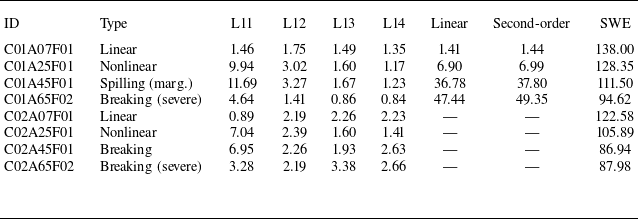
Generally, the differences observed among the three highest levels of refinement are minimal, confirming convergence regarding surface elevation. However, at refinement level 11, a noticeable decline in performance is observed. The best results are obtained for the 25 mm linear amplitude test conditions, which represent weakly nonlinear waves. Although it might be anticipated that the linear test cases (7 mm amplitude) would perform equally well, the very low amplitude renders these conditions more challenging due to a low signal-to-noise ratio in the model test measurements. Given that benchmark errors are reported relative to the amplitude, these results are not surprising.
For the steepest conditions tested, the benchmark results are slightly inferior to those for the weakly nonlinear case, yet remain robust across the three highest levels of refinement, particularly considering that these conditions are strongly nonlinear and involve wave breaking. Comparisons of wave elevation measurements for different refinement levels under test conditions C02A25F01 and C02A65F02 are illustrated in figure 13, visually corroborating the findings indicated by the benchmark results.
Comparison of wave elevation $\hat {\eta }$
, computed using different grid refinement levels, for almost linear (a) and severely breaking (b) conditions.
$\hat {\eta }$
, computed using different grid refinement levels, for almost linear (a) and severely breaking (b) conditions.

In contrast, the performance of linear wave theory demonstrates a marked deterioration as the amplitude increases, as previously observed in the wave elevation comparisons shown in figures 5 and 6.
The benchmark errors obtained with second-order irregular wave theory are very similar to those of the linear theory across the C01 series, and likewise deteriorate sharply with increasing amplitude. Although second-order theory produces a more realistic crest–trough asymmetry and bound-wave structure than the linear model, it does not capture the nonlinear amplitude and frequency modulation that develops as a dispersive wave group steepens and approaches focus. In the benchmark metric, where the elevation is sampled at fixed gauge positions and weighted by the experimental amplitude, the residual error is therefore dominated by a phase offset between the numerical and experimental wave groups, and is only weakly reduced by the improved wave shape. This is visible in the surface-elevation comparisons in figure 15.
The SWE model, by contrast, produces benchmark errors that are two to three orders of magnitude larger than those of the Navier–Stokes model and do not improve with increasing amplitude. Because the shallow-water equations assume a hydrostatic pressure distribution, they are non-dispersive, and all frequency components propagate at the long-wave celerity $c = \sqrt {gh}$
. For the deep- and intermediate-depth conditions considered here this assumption is fundamentally violated: the individual spectral components no longer travel at their respective linear phase speeds, and the focused wave group cannot be reproduced. The effect is already evident at wave gauge 1, only
$c = \sqrt {gh}$
. For the deep- and intermediate-depth conditions considered here this assumption is fundamentally violated: the individual spectral components no longer travel at their respective linear phase speeds, and the focused wave group cannot be reproduced. The effect is already evident at wave gauge 1, only $\approx 1\,\textrm{m}$
from the paddle, where the SWE solution has already lost its prescribed amplitude and phase structure, as shown in figures 15 and 16. The SWE entries in table 2 are included as a baseline illustrating the penalty incurred when a non-dispersive model is applied outside its intended regime of validity.
$\approx 1\,\textrm{m}$
from the paddle, where the SWE solution has already lost its prescribed amplitude and phase structure, as shown in figures 15 and 16. The SWE entries in table 2 are included as a baseline illustrating the penalty incurred when a non-dispersive model is applied outside its intended regime of validity.
Finally, we evaluated the contribution of the various wave gauges to the reference error $\epsilon$
, as shown in table 3. The percentage contributions are averaged across all eight test conditions and were found to be relatively consistent across the different cases. As anticipated, the contribution from wave gauge 1 is negligible due to its proximity to the wave maker. The most significant contributions arise from wave gauges 2 and 3, which can be attributed to the occurrence of wave breaking in that area, making it difficult to accurately measure surface elevation in the experiments using acoustic probes and in the CFD model due to air–water mixing. However, once the wave groups reach wave gauge 4, measurements become easier, resulting in a lower error.
$\epsilon$
, as shown in table 3. The percentage contributions are averaged across all eight test conditions and were found to be relatively consistent across the different cases. As anticipated, the contribution from wave gauge 1 is negligible due to its proximity to the wave maker. The most significant contributions arise from wave gauges 2 and 3, which can be attributed to the occurrence of wave breaking in that area, making it difficult to accurately measure surface elevation in the experiments using acoustic probes and in the CFD model due to air–water mixing. However, once the wave groups reach wave gauge 4, measurements become easier, resulting in a lower error.
The contribution to the benchmark error $\epsilon$
from different wave probes. The result is found to be quite consistent for all levels of refinement.
$\epsilon$
from different wave probes. The result is found to be quite consistent for all levels of refinement.

4.8. Computational performance
The computational cost of CFD wave models depends on the level of simulation refinement, as well as the resulting velocities in the fluid flow. Our wave model is no different. The time step of the iterative solver is controlled by the CFL number, which may be seen as an expression of the maximum distance that a particle is allowed to move relative to the size of the cell through which it moves in a time step. The CFL number for our simulations was set to 0.1 for all cases to ensure energy convergence. The simulations were run on FRAM, one of Norwegian Research Infrastructure Services (NRIS) high-performance computational clusters, with Intel E5-2683v4 2.1 GHz nodes, each of which has 32 threads available. Since the number of cells in the domain varies over time due to AMR, the number of threads utilised varies between 2 and 32, during runtime, to optimise performance. The total simulation time accumulated (wall clock) is calculated as
 \begin{equation} t_{awc} = t_{wallclock} \bar {N}_{thread}, \end{equation}
where $t_{wallclock}$
is the simulation time (wall clock) and
$t_{wallclock}$
is the simulation time (wall clock) and $\bar {N}_{thread}$
is the average, time-weighted, number of threads used during the simulation. The accumulated simulation times (in hours) for all the simulated cases are presented in table 4.
$\bar {N}_{thread}$
is the average, time-weighted, number of threads used during the simulation. The accumulated simulation times (in hours) for all the simulated cases are presented in table 4.
Accumulated simulation time $t_{awc}$
, computed for all simulated cases. Values are given in number of hours.
$t_{awc}$
, computed for all simulated cases. Values are given in number of hours.

It is evident that the computational cost of simulating each event varies significantly, both across different refinement levels and among individual cases, depending on the steepness of the conditions. Although the three highest grid refinement levels generally yield very similar results, it is noteworthy that the cost of running the steepest conditions at level 12 is less than 5 % of that at level 14.
5. Conclusion
A novel experimental dataset specifically designed for deterministic validation of numerical wave models has been presented. This compact dataset, comprising eight test cases, encompasses a wide range of conditions, from low-steepness dispersive waves in deep water to steep breaking waves over a variable seabed. By propagating dispersive focused wave groups over multiple wavelengths, this dataset provides a robust framework for assessing the ability of numerical wave models to simulate dispersive wave propagation in both open ocean (deep water) and coastal (variable and shallow water) environments.
Using the two-phase flow volume-of-fluids Navier–Stokes wave model described in § 3, we demonstrate that the experimental results can be deterministically recreated with a satisfactory level of accuracy using only the prescribed paddle motion as the boundary input. This finding corroborates the excellent conservation properties of the numerical model, and its ability to model the complex two-phase flow of breaking waves.
As part of the validation process, we conducted simulations with varying grid resolutions to evaluate the convergence of different wave properties. We compared the wave elevations, kinematics, momentum flux and energy dissipation resulting from wave breaking. The results indicate that the numerical wave model is generally proficient in replicating the experimental observations, even under the steepest breaking conditions tested. Notably, the minor differences in energy dissipation observed across the three highest levels of grid refinement were unexpected; all three resolutions yielded results closely aligned with the experimental data, despite the fact that the selected grid resolutions did not fully resolve all turbulent scales. This outcome is particularly encouraging, considering that achieving very high grid resolutions can be computationally prohibitive when modelling short-crested wave fields within a three-dimensional domain.
Lastly, we propose a straightforward benchmarking method for evaluating the performance of our wave model aimed at differentiating and comparing the capabilities of various wave models. In this study, we opted for an advanced wave model to maximise our chances of accurately reproducing the experimental results. However, the computational costs associated with such models, as illustrated in § 4.8, can be substantial and can become prohibitive when extended to larger three-dimensional domains. Consequently, the experimental dataset presented is intended for the validation of less sophisticated wave models, allowing for an exploration of their limitations in modelling the complexities inherent in ocean and coastal wave dynamics. To facilitate broader accessibility, the experimental dataset is published as open access.
Beyond the three reference models considered in the present work (linear and second-order irregular wave theory and the SWE model), the benchmark is deliberately designed to be applicable to a wide class of phase-resolved wave models, including Boussinesq, multi-layer, higher-order spectral and boundary-element formulations. We therefore encourage other researchers to apply the dataset and the proposed benchmark metric to their own models, and to contribute their results as further reference points. In this way the dataset can grow into a shared basis for systematic, cross-model comparison of the ability to propagate dispersive wave groups over long distances, through varying bathymetry, and into the breaking regime.
Acknowledgements
Computational resources for this project were provided by Norwegian Research Infrastructure Services (NRIS), for which we are very grateful. We have used LLM-powered tools (Overleaf, Writefull) to improve language quality and correctness. All the scientific content is the result of the work of the authors, and the authors checked and quality-controlled all LLM-produced language edits.
Funding
The work was supported by the Norwegian Research Council and Ocean Oasis AS, as part of the industrial PhD programme.
Declaration of interests
The authors report no conflict of interest.
Data availability statement
The experimental dataset is published open access in the University of Oslo’s data repository DataverseNO (Lande Reference Lande2026), and is available at https://doi.org/10.18710/FZN3AL. The archive includes the raw PIV velocity fields, the full wave-gauge records for all repetitions, the paddle motion signals and the raw and processed time series used in the paper.
Appendix A. Wall friction assessment
In the present configuration where we assessed wall friction (configuration C01), the water depth is large compared with the wavelength of the energetic components of the focused wave group, so bottom friction is negligible. The measured non-breaking dissipation of $\approx 1.5\,\%$
per mean wavelength (figure 2) must therefore originate from processes localised at the side walls: the viscous boundary layers on the glass, capillary-scale contact-line damping and the small parasitic ripples observed along the contact line as the wave group passes (see also Hunt Reference Hunt1952). Because these contributions cannot be separated in the integrated surface-elevation budget, the calibrated coefficient
$\approx 1.5\,\%$
per mean wavelength (figure 2) must therefore originate from processes localised at the side walls: the viscous boundary layers on the glass, capillary-scale contact-line damping and the small parasitic ripples observed along the contact line as the wave group passes (see also Hunt Reference Hunt1952). Because these contributions cannot be separated in the integrated surface-elevation budget, the calibrated coefficient $c_f = 0.0119$
lumps them into a single linear dissipation model. The amplitude-independence of the measured dissipation rate (figure 2) supports the use of a linear closure in the non-breaking regime.
$c_f = 0.0119$
lumps them into a single linear dissipation model. The amplitude-independence of the measured dissipation rate (figure 2) supports the use of a linear closure in the non-breaking regime.
To assess whether this calibration remains representative once the wave group steepens and breaks, we characterise the flow at the wall by the oscillatory-flow Reynolds number
 \begin{equation} Re_w = \frac {U_m a}{\nu _w}, \end{equation}
where $U_m$
is the maximum near-surface orbital velocity and
$U_m$
is the maximum near-surface orbital velocity and $a$
the corresponding orbital excursion (Jensen, Sumer & Fredsøe Reference Jensen, Sumer and Fredsøe1989). For the focused wave group with mean wavenumber
$a$
the corresponding orbital excursion (Jensen, Sumer & Fredsøe Reference Jensen, Sumer and Fredsøe1989). For the focused wave group with mean wavenumber $k_m = 6.4\,\textrm{m}^{-1}$
and mean angular frequency
$k_m = 6.4\,\textrm{m}^{-1}$
and mean angular frequency $\omega _m = 7.95\,\textrm{rad s}^{-1}$
, the three representative amplitudes give the values listed in table 5. In the breaking case,
$\omega _m = 7.95\,\textrm{rad s}^{-1}$
, the three representative amplitudes give the values listed in table 5. In the breaking case, $U_m$
is replaced by the crest velocity at the point of overturning, which approaches the phase speed of the wave group.
$U_m$
is replaced by the crest velocity at the point of overturning, which approaches the phase speed of the wave group.
Wall-boundary-layer Reynolds number for the three characteristic amplitudes of the focused wave group. The non-breaking cases span the laminar-to-transitional regime of the oscillatory boundary layer, whereas the breaking case lies well within the turbulent regime (Jensen et al. Reference Jensen, Sumer and Fredsøe1989).

The non-breaking cases in which $c_{\!f}$
was calibrated therefore cover
$c_{\!f}$
was calibrated therefore cover $Re_w \sim 10^{2}$
–
$Re_w \sim 10^{2}$
– $10^{4}$
, which for oscillatory boundary layers on smooth walls corresponds to the laminar-to-transitional regime (Jensen et al. Reference Jensen, Sumer and Fredsøe1989). The breaking case, by contrast, lies well into the turbulent regime, where the wave-friction factor is known to depend on
$10^{4}$
, which for oscillatory boundary layers on smooth walls corresponds to the laminar-to-transitional regime (Jensen et al. Reference Jensen, Sumer and Fredsøe1989). The breaking case, by contrast, lies well into the turbulent regime, where the wave-friction factor is known to depend on $Re_w$
and on wall roughness. Strictly speaking, the calibrated coefficient is therefore representative only of the laminar-to-transitional range in which it was obtained.
$Re_w$
and on wall roughness. Strictly speaking, the calibrated coefficient is therefore representative only of the laminar-to-transitional range in which it was obtained.
It is nevertheless important to recognise that a dispersive focused wave group is, by construction, only focused at a single location in the tank. Over the remainder of the propagation distance the wave components are dispersed and the local orbital velocities are substantially lower than the peak value at focus. The turbulent-regime Reynolds number reported for the breaking case in table 5 is therefore attained only in a limited region around the breaking point, while along the majority of the propagation length the flow at the wall remains in the same laminar-to-transitional regime in which $c_{\!f}$
was calibrated. In addition, in the breaking cases the wall-friction budget is small compared with the energy lost to wave breaking itself (figure 12
a), so that the associated modelling error is bounded above by the
$c_{\!f}$
was calibrated. In addition, in the breaking cases the wall-friction budget is small compared with the energy lost to wave breaking itself (figure 12
a), so that the associated modelling error is bounded above by the $\approx 1.5\,\%$
-per-wavelength dissipation quantified in the non-breaking measurements. A single value of
$\approx 1.5\,\%$
-per-wavelength dissipation quantified in the non-breaking measurements. A single value of $c_{\!f}$
is therefore retained throughout the simulations, and the uncertainty introduced by this choice in the breaking regime is acknowledged as a limitation.
$c_{\!f}$
is therefore retained throughout the simulations, and the uncertainty introduced by this choice in the breaking regime is acknowledged as a limitation.
Because $c_{\!f}$
is calibrated directly against the measured non-breaking dissipation rate (figure 2), its value is fixed once and not further adjusted when comparing with individual test cases. The value of
$c_{\!f}$
is calibrated directly against the measured non-breaking dissipation rate (figure 2), its value is fixed once and not further adjusted when comparing with individual test cases. The value of $c_{\!f}$
controls the amount of energy delivered to focus: a larger
$c_{\!f}$
controls the amount of energy delivered to focus: a larger $c_{\!f}$
removes too much energy and delays or suppresses breaking, whereas a smaller
$c_{\!f}$
removes too much energy and delays or suppresses breaking, whereas a smaller $c_{\!f}$
delivers too much energy at focus and triggers premature breaking with an inflated crest amplitude. Consistency between the experimental and numerical wave groups at the measurement stations therefore requires that
$c_{\!f}$
delivers too much energy at focus and triggers premature breaking with an inflated crest amplitude. Consistency between the experimental and numerical wave groups at the measurement stations therefore requires that $c_{\!f}$
reflects the measured tank dissipation rather than be adjusted to minimise residuals in the surface-elevation comparison.
$c_{\!f}$
reflects the measured tank dissipation rather than be adjusted to minimise residuals in the surface-elevation comparison.
Appendix B. Grid resolution and energetics
The flow problem of wave propagation with high density ratios between air and water, combined with shear flow over the surface boundary, makes it numerically challenging, as discussed by Desjardins & Moureau (Reference Desjardins and Moureau2010) and Remmerswaal (Reference Remmerswaal2023). For this reason, we evaluate the performance of our numerical wave model for a wide range of grid resolutions, as presented in table 6. Up to the point of breaking and overturning, wave evolution is well described by potential flow solvers (Grilli et al. Reference Grilli, Dias, Guyenne, Fochesato and Enet2010). The velocity field is essentially irrotational and inviscid, and no turbulence or viscous layers should need to be resolved at a very high resolution in order to get good agreement between experiments and numerical models. However, during breaking, vorticity and air and water mixing turn the flow field in the vicinity of the surface into a complex turbulent two-phase flow problem (see Lubin & Glockner Reference Lubin and Glockner2015; Deike et al. Reference Deike, Melville and Popinet2016; Remmerswaal Reference Remmerswaal2023). What follows is the dissipation of turbulent kinetic energy, which occurs at the smallest scales of flow, commonly described by the Kolmogorov length scale $\eta _v$
in the turbulence flow theory (see Landahl & Mollo-Christensen Reference Landahl and Mollo-Christensen1992). Accurately resolving these scales in our simulation requires a significantly higher grid resolution than that necessary for wave evolution in the pre-breaking phase. To estimate the resolved length scales for the various grid resolutions employed, we can compute a conservative estimate of the Kolmogorov length scale given by
$\eta _v$
in the turbulence flow theory (see Landahl & Mollo-Christensen Reference Landahl and Mollo-Christensen1992). Accurately resolving these scales in our simulation requires a significantly higher grid resolution than that necessary for wave evolution in the pre-breaking phase. To estimate the resolved length scales for the various grid resolutions employed, we can compute a conservative estimate of the Kolmogorov length scale given by
Grid refinement levels used when assessing the performance of the numerical wave model.

 \begin{equation} \eta _v = \left (\frac {\nu _w^3}{\varepsilon }\right )^{1/4}, \end{equation}
where $\nu _w$
is the kinematic viscosity of water and
$\nu _w$
is the kinematic viscosity of water and $\varepsilon$
represents the energy dissipation rate.
$\varepsilon$
represents the energy dissipation rate.
In the context of breaking waves, the dissipation rate varies spatially and temporally, making it impossible to calculate a priori for the simulation, as highlighted by Vollestad, Ayati & Jensen (Reference Vollestad, Ayati and Jensen2019). Nonetheless, the average dissipation rate in breaking waves has been extensively investigated (see Rapp & Melville Reference Rapp and Melville1990; Banner & Peirson Reference Banner and Peirson2007; Drazen et al. Reference Drazen, Melville and Lenain2008; Tian et al. Reference Tian, Perlin and Choi2010). For a conservative estimate, we use a dissipation rate approximately ten times the largest average value reported by Banner & Peirson (Reference Banner and Peirson2007), which results in $\varepsilon \approx 0.026\, \text{m}^2\,\text{s}^{-3}$
. This value aligns well with a similar conservative estimate provided by Vollestad et al. (Reference Vollestad, Ayati and Jensen2019) in their calculations of the Kolmogorov length scale under wave conditions. The Kolmogorov criterion is considered satisfied if
$\varepsilon \approx 0.026\, \text{m}^2\,\text{s}^{-3}$
. This value aligns well with a similar conservative estimate provided by Vollestad et al. (Reference Vollestad, Ayati and Jensen2019) in their calculations of the Kolmogorov length scale under wave conditions. The Kolmogorov criterion is considered satisfied if $\eta _v k_{max} \geqslant 1$
, where
$\eta _v k_{max} \geqslant 1$
, where $k_{max} = {2^N\pi }/{L}$
represents the maximum resolved wavenumber of the computational grid.
$k_{max} = {2^N\pi }/{L}$
represents the maximum resolved wavenumber of the computational grid.
Additionally, a second criterion concerns the adequate resolution of the boundary layer at the free surface, which is crucial to accurately modelling the shear flow that contributes to vorticity generation. Following Deike, Popinet & Melville (Reference Deike, Popinet and Melville2015), the thickness of this viscous sublayer can be approximated by $\delta \approx {\lambda }/{\sqrt {Re}}$
, where
$\delta \approx {\lambda }/{\sqrt {Re}}$
, where $\lambda$
is the mean wavelength and
$\lambda$
is the mean wavelength and $Re$
is the Reynolds number. Mostert & Deike (Reference Mostert and Deike2020) found that a minimum of four cells within the width of the boundary layer is sufficient for numerical convergence, leading to the boundary-layer criterion of
$Re$
is the Reynolds number. Mostert & Deike (Reference Mostert and Deike2020) found that a minimum of four cells within the width of the boundary layer is sufficient for numerical convergence, leading to the boundary-layer criterion of $\delta /\Delta x \geqslant 4$
.
$\delta /\Delta x \geqslant 4$
.
The results for both criteria and their associated parameters are presented in table 7 for the range of refinement levels under consideration. The results of these criteria are highlighted in bold. It is clear that even at the highest refinement level, the resolution remains insufficient to completely resolve all turbulent scales and the thickness of the viscous sublayer. This finding is particularly noteworthy, given that we are only examining laboratory waves at scales considerably lower than those of the ocean environment that we aim to model. Thus, claiming grid convergence with a direct numerical simulation model, such as the one employed in this study, in the context of modelling breaking ocean waves may be, at best, misleading.
Turbulent scales and viscous sublayer assessment criteria assessment presented for different levels of refinement (for each level, the cell size is reduced by a factor of 2).

Normalised wave-group potential energy $E_p/E_{p,0}$
as a function of propagation distance for condition C01A25F01 at refinement level 13, for a range of CFL numbers. The energy is computed from the simulated surface elevation at each wave gauge using (2.5). The curves collapse for
$E_p/E_{p,0}$
as a function of propagation distance for condition C01A25F01 at refinement level 13, for a range of CFL numbers. The energy is computed from the simulated surface elevation at each wave gauge using (2.5). The curves collapse for $C \leqslant 0.3$
, demonstrating convergence with respect to the CFL number at this grid resolution.
$C \leqslant 0.3$
, demonstrating convergence with respect to the CFL number at this grid resolution.

Comparison of normalised wave elevation for the four constant-deep-water test cases, obtained with second-order irregular wave theory and with the SWE model: (a) linear, (b) weakly nonlinear, (c) steep at the limit of breaking and (d) severely breaking.

Since we have chosen to limit our simulation to a two-dimensional framework for practical reasons, further refinement is feasible. However, turbulent flow is indeed a three-dimensional problem and it would become increasingly impractical to increase resolution when transitioning to three-dimensional simulations. Therefore, exceeding the grid resolutions indicated in table 7 is not considered practical. Nevertheless, as noted by Siddiqui & Loewen (Reference Siddiqui and Loewen2007), complete resolution of all Kolmogorov scales is not required to obtain an accurate estimate of energy dissipation. A more thorough examination of energy dissipation will be conducted in a comparison between the experimental results and the numerical simulations.
Comparison of wave elevation for the two breaking conditions over the shoal for C02A45F01 (a) and C02A65F02 (b), obtained with the SWE model. Grey dots show the corresponding experiment without the shoal, for reference.

Appendix C. The CFL sensitivity
The explicit time integration in Basilisk is constrained by the CFL condition, and the chosen CFL number $C$
directly sets the time-step size relative to the local grid spacing and flow velocity. Because the simulations cover long propagation distances (tens of wavelengths) and rely on accurate preservation of the wave energy prior to focusing, the sensitivity of the solution to
$C$
directly sets the time-step size relative to the local grid spacing and flow velocity. Because the simulations cover long propagation distances (tens of wavelengths) and rely on accurate preservation of the wave energy prior to focusing, the sensitivity of the solution to $C$
was assessed before the production runs.
$C$
was assessed before the production runs.
The representative non-breaking focused wave group C01A25F01 was simulated at refinement level 13 for a range of CFL numbers, with all other numerical parameters held fixed. The potential energy of the wave group was then evaluated from the simulated surface elevation at the four wave gauges using the same time-integrated estimator (2.5) introduced in § 2.5.1, and the normalised energy loss $E_p/E_{p,0}$
was tracked along the
$E_p/E_{p,0}$
was tracked along the $\approx 9$
m propagation distance from wave gauge 1 to wave gauge 4, using
$\approx 9$
m propagation distance from wave gauge 1 to wave gauge 4, using $E_{p,0}$
taken at wave gauge 1.
$E_{p,0}$
taken at wave gauge 1.
The results are shown in figure 14. A monotonic increase in energy loss is observed as the CFL number is increased, reflecting accumulated time-discretisation error in the projection step. The curves collapse for $C \leqslant 0.3$
, indicating that the numerical dissipation associated with the time integration has become negligible relative to the remaining physical and numerical sources of energy dissipation at this grid resolution – namely, fluid viscosity and numerical damping from the spatial discretisation. Further reduction of
$C \leqslant 0.3$
, indicating that the numerical dissipation associated with the time integration has become negligible relative to the remaining physical and numerical sources of energy dissipation at this grid resolution – namely, fluid viscosity and numerical damping from the spatial discretisation. Further reduction of $C$
below this value therefore yields no measurable improvement. The conservative value
$C$
below this value therefore yields no measurable improvement. The conservative value $C = 0.1$
was adopted as the production setting, providing a comfortable margin inside the converged plateau while keeping the time-step cost acceptable.
$C = 0.1$
was adopted as the production setting, providing a comfortable margin inside the converged plateau while keeping the time-step cost acceptable.
Taken together with the grid-refinement study (figure 11 and table 7 and the benchmark error tables in the main text), this confirms that the numerical parameters employed in the production runs lie in a regime where neither the spatial nor the temporal discretisation is the dominant source of error in the comparison with the experiment.
Appendix D. Comparative validation with second-order and shallow-water models
For completeness, and to complement the benchmark error reported in table 2, this appendix reproduces the surface elevation comparisons of figures 5(a), 6(a) and 8(a) using two additional reference models: second-order irregular wave theory and a depth-averaged SWE solver. The constant deep-water cases (C01 series) are collected in figure 15, and the shoal cases (C02 series) in figure 16. The same paddle-motion boundary condition and the same four wave gauges are used as in the experiments, so that the comparisons are directly analogous to those of the CFD model in the main text.
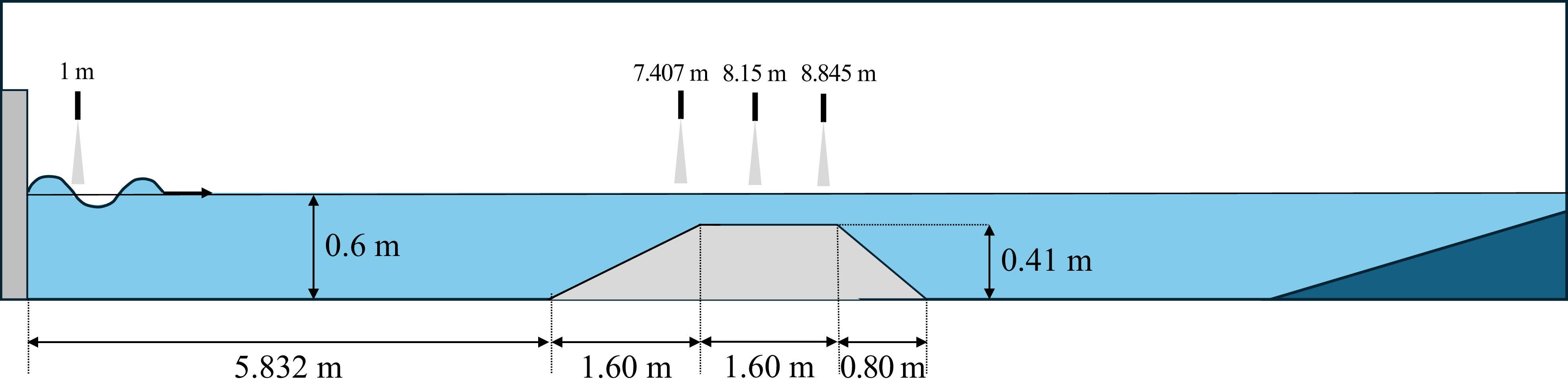
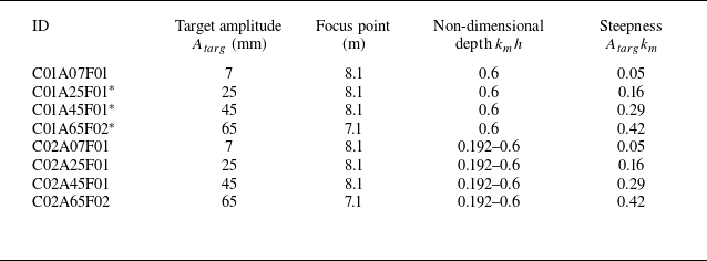
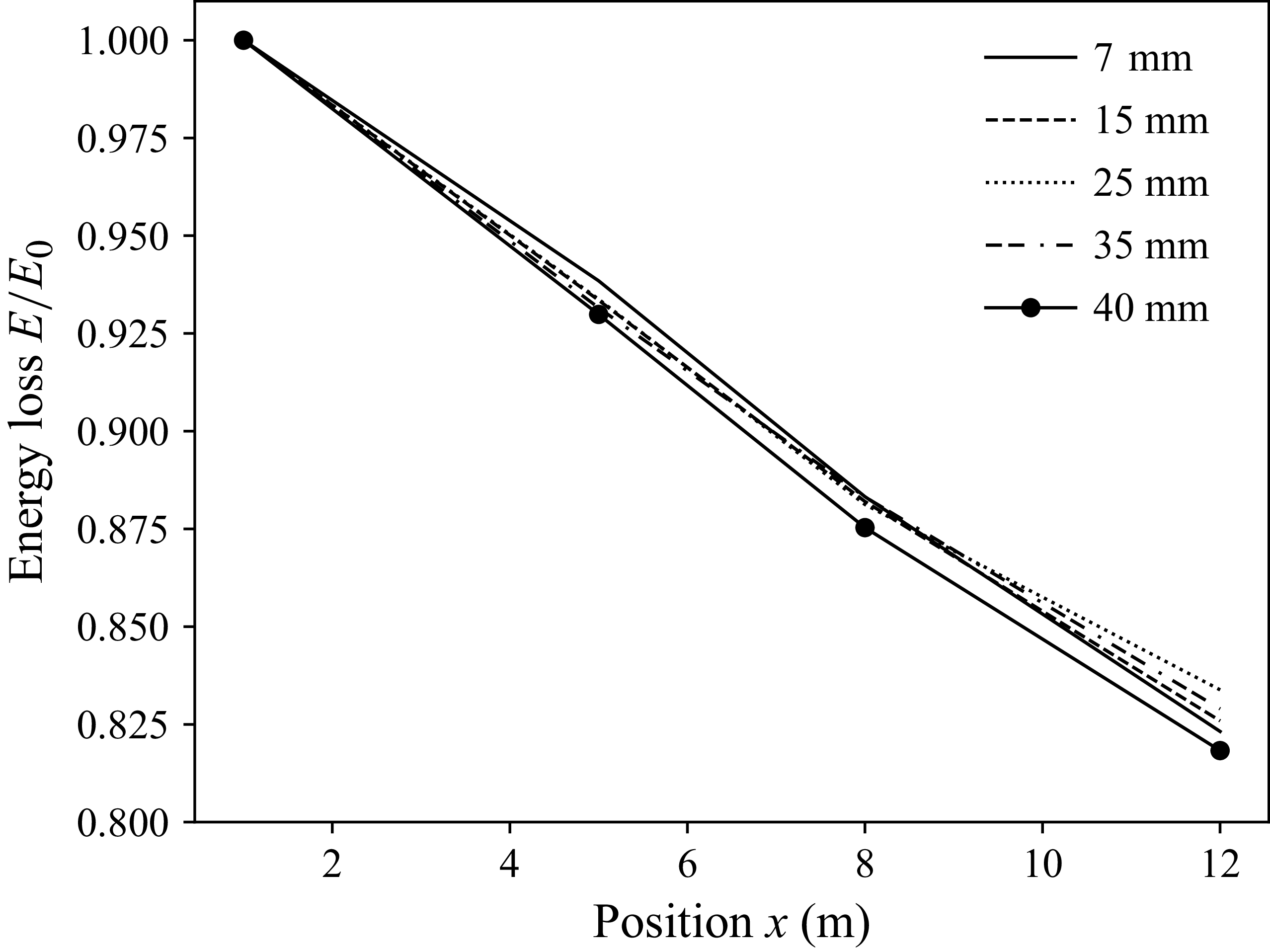


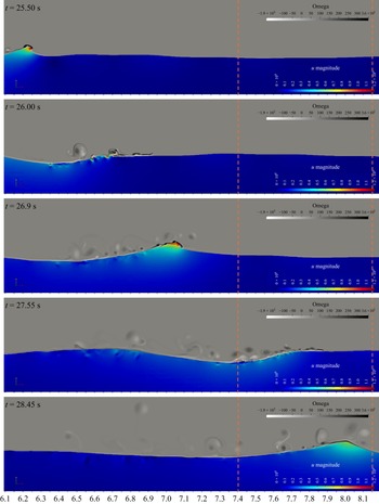

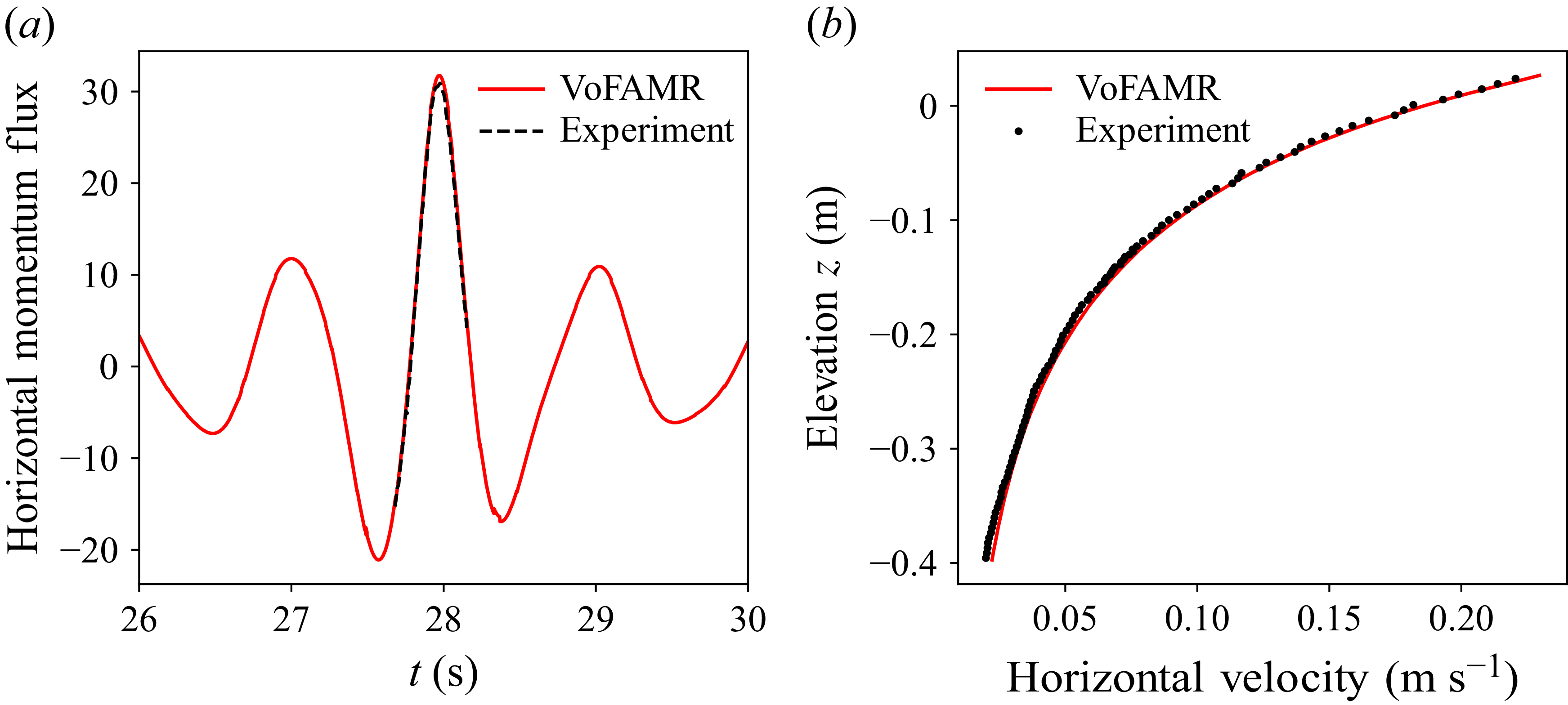
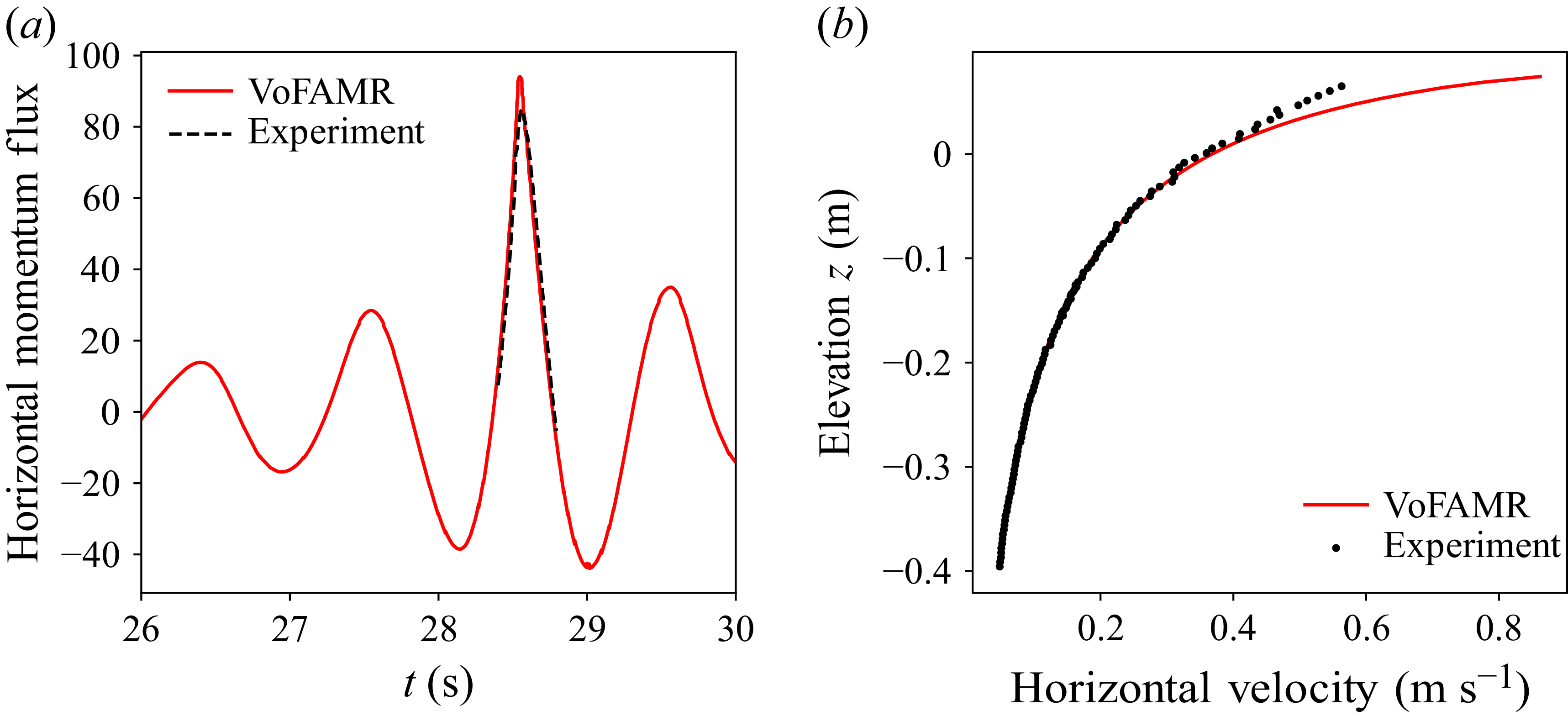


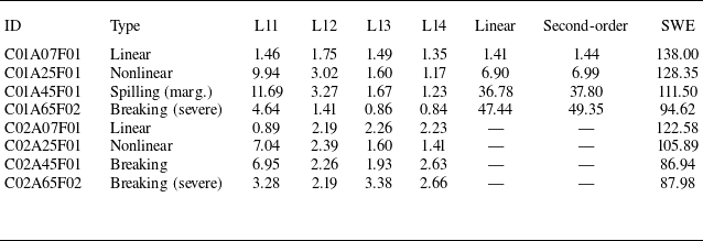


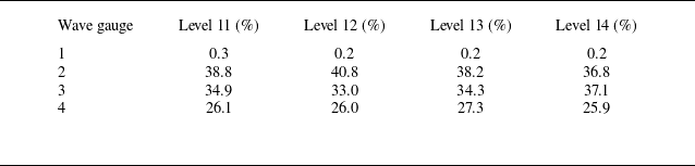

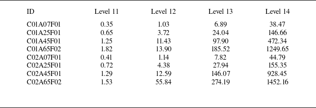

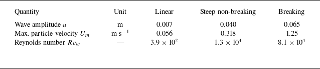
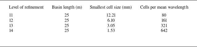
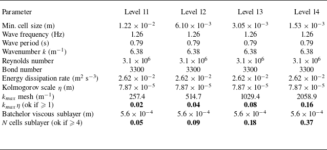
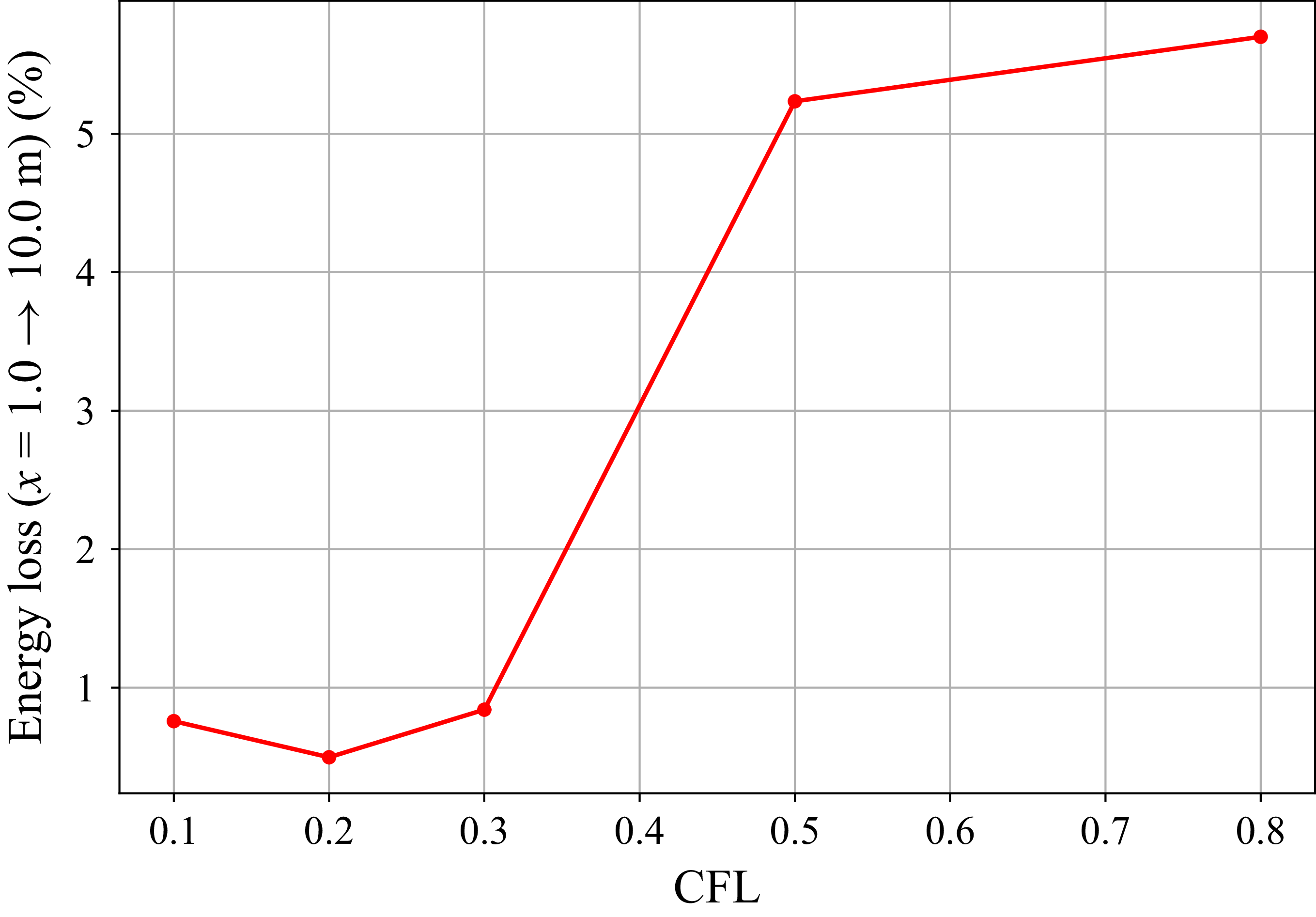


 Open access

