

I
Russia’s invasion of Ukraine in February 2022 triggered a surge in energy prices, increasing inflation in the euro area and other advanced countries. Inflation was already rising due to the post-Covid-19 recovery, driven by increased demand and supply chain bottlenecks. The Ukraine conflict exacerbated these pressures, particularly through war-induced energy price hikes.
Historically, the 1970s are often taken as a reference point to investigate the effects on inflation of abrupt energy supply shocks and associated policy responses. This decade marked the end of the strong economic growth experienced during the Bretton Woods era.Footnote 1 After the collapse of the gold exchange standard regime set up at the end of World War II, the world economy was hit by large increases in the price of oil triggered by two episodes: the Yom Kippur War in 1973 and the Iranian Revolution in 1979. Oil prices quadrupled in 1973–4, and more than doubled in 1979–80, fueling a sharp rise in inflation. As Goodfriend (Reference Goodfriend2007) noted regarding the US, monetary policy was in ‘disarray’Footnote 2 and failed to control inflation for nearly a decade (with the notable exception of Germany). The initial monetary response to the first oil shock was too weak, necessitating a stronger response to the second shock, which negatively affected economic growth.Footnote 3
However, the stance of monetary policy alone seems insufficient to fully explain the high and persistent levels of inflation, as well as the significant differences in inflation rates across advanced economies. In this article, we examine three institutional factors that distinguish the recent inflation episode from the 1970s, which most likely prevented the 2022 energy shock from leading to inflation as high and persistent as 50 years ago.
The first factor concerns the framework in which monetary policy operates. After the collapse of the fixed exchange rate regime and the gold peg in 1971, monetary policy lacked a clear framework. In this context, countries characterized by a higher level of central bank independence had significantly better inflation outcomes. A new conduct framework would only be established over the next two decades overall, initially moving toward announcing the future course of key nominal variables as intermediate targets (exchange rates, but more often monetary targets) as a way to influence inflation expectations. Then, as the demand for money became increasingly unstable due to financial innovation, it became evident that, although highly correlated in the long run, money and inflation were not sufficiently correlated in the short run, and monetary policy progressively shifted (since the 1990s) toward a strategy based on the commitment by independent and credible central banks to achieve well-identified quantitative inflation targets (Croce and Kahn Reference Croce and Kahn2000; Goodfriend Reference Goodfriend2007).
The second aspect relates to labor market bargaining processes characterized by high conflictuality and by wage-setting mechanisms disconnected from the dynamics of labor productivity, which fostered wage-price spirals via automatic wage indexation to prices. The third factor is fiscal policy, which often conflicted with price stability goals
In this article, we analyze these factor and quantitatively assess the role they had in sustaining inflation persistence in the 1970s. In Section II we describe the dynamics of inflation, GDP and the monetary policy responses (in terms of official rates) given in the 1970s to the oil shocks, comparing the experience of three selected countries (the United States, Germany and Italy). In Section III we review the literature on macroeconomic and monetary policy history, underlying the evolution of the framework under which monetary policy operated. In Section IV we argue why the aforementioned institutional factors explain the significant cross-countries heterogeneity in inflation performance during the 1970s, and provide supporting descriptive evidence. Section V provides a time-series econometric assessment: using a structural VAR model, we perform a counterfactual analysis focusing on Italy, Germany, the US and the UK, and identify the contribution of monetary policy, wage dynamics and fiscal policy to the stubborn inflation of the 1970s. Section VI concludes.
II
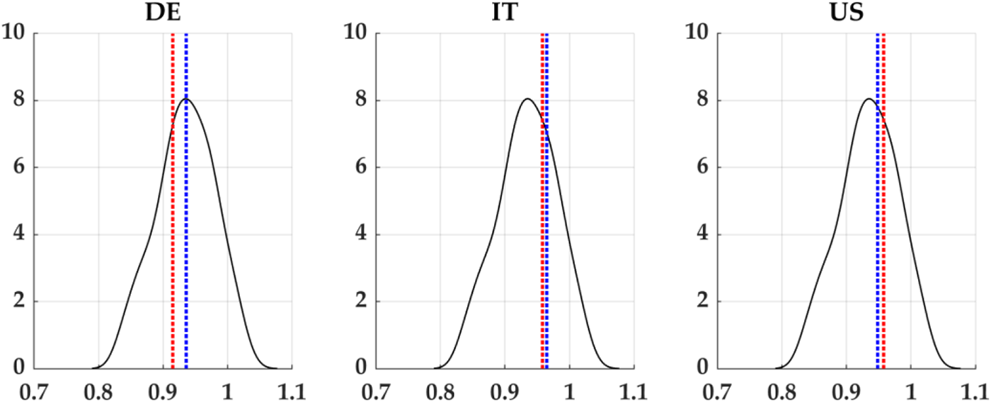
Following the 1973 and the 1979 shocks, oil prices first quadrupled, then more than doubled (Figure 1), fueling inflation across most advanced countries (Figure 2). A concerning feature of these price dynamics, beyond their speed and magnitude, was their persistence. Figure 3 shows the time-varying persistence of inflation, computed as the parameter of a univariate time-varying autoregressive model with stochastic volatility:Footnote 4 the black line is the distribution of persistence across seven member countries of the Organization for Economic Cooperation and Development (OECD) while dotted vertical lines represent country-specific inflation persistence in the 1973–7 (red line) and the 1978–82 (blue line) periods for the United States, Germany and Italy. Both Italy and the US exhibit a higher than average inflation persistence while in Germany, which behaved quite differently compared to the other countries considered, persistence was significantly lower both after the first and after the second shock. As shown in Figure 4, in Germany, inflation and persistence both declined after the 1973 shock. Persistence increased later, but only after inflation stabilized around 4 percent per year.Footnote 5 In Italy, inflation remained high between the two shocks, and after the second shock, inflation persistence gradually diminished, becoming more homogeneous across countries. After the second shock, the degree of persistency slowly diminished becoming more homogeneous across countries.
Spot Crude (WTI) Oil price level and growth, 1960–85 Source: FRED, Federal Reserve Bank of St. Louis.

Consumer inflation in selected countries, 1960–2022 Source: BIS Statistics Warehouse.

Inflation persistence in selected countries: 1973–7 versus 1978–82

Inflation persistence in selected countries, 1965–85

Official policy rates, our measure of monetary policy reaction,Footnote 6 were already rising before the first oil shock (less so in Italy), in line with inflation: however, the immediate post-shock response looks relatively small (Figure 5). Subsequently, the interest rate reduction was rapid: in the US the Federal funds rate rose after 1973 but then reached pre-shock levels as soon as late 1974 (supposedly because of concerns related to economic growth), just one year after the outbreak of the Yom Kippur War.Footnote 7 In Italy, the initial rise in the policy rate was quickly reabsorbed after five quarters. Inflation in Germany seems not to have been particularly affected by the oil shock, and monetary conditions were eased in late 1974.
Policy rates in selected countries, 1960–85

In both the US and Germany, a neutral monetary policy stance was reached before the second oil shock, followed by a restrictive stance thereafter. Italy followed this shift with some delay (Figure 6), helping to curb inflation, though with varying timing.Footnote 8
Monetary policy stance (ex-post real interest rate) Note: Ex-post real interest rates represent a simple and model-independent measure of the monetary policy stance: ECB (2010).

The US and Germany experienced a severe drop in aggregate demand and fell into a double-dip recession between 1981 and 1983 (Figure 7). In Italy, real GDP fell after the first shock when monetary policy did not respond aggressively, while growth only slowed down after the second shock when the policy response was tighter. These differentiated pictures do not help to shed light on the effectiveness of monetary policy and on the extent to which recessions were eased by the monetary policy reaction.Footnote 9 In the last section of the present work we’ll measure quantitatively this effects with a structural vector autoregressive (SVAR) analysis.
GDP, inflation and policy rates in selected countries, 1960–85

To summarize the three cases analyzed, they differ in key aspects. In the US, after the first shock, inflation gradually converged to pre-shock levels despite a weak initial monetary response, though a premature easing may have contributed to inflation persistence. The Volcker era followed and attacked inflation as the main enemy. In Germany, inflation increased ‘mildly’ after the first oil shock. Conversely, the second shock was associated with an increase in inflation that was dealt with by means of a sharp increase in the policy rates. Italy’s inflation, already on the rise before the first oil shock, jumped higher after 1973. The country was not able to curb inflation during the 1970s with a scant monetary policy reaction (limited by scarce operational autonomyFootnote 10) and struggled to bring inflation down in the 1980s.
Overall, a relatively accommodative monetary policy stance followed the first oil shock, with a stronger tightening after the second shock proving effective in combating inflation. However, both shocks had severe negative effects on growth. Germany saw better inflation control, especially after the first shock, when inflation peaked at 7 percent and quickly declined. In contrast, Italy’s inflation peaked at 20 percent and remained high, while US inflation showed significant persistence, reaching 13.5 percent in 1980.
Clarida, Galí and Gertler (Reference Clarida, Galí and Gertler2000) claim that there has been a significant change in how monetary policy was conducted before and after 1979, and that this regime shift proved finally to be effective in reducing inflation in the 1980s.Footnote 11 Sims and Zha (Reference Sims and Zha2006) identify such a regime shift too, but conclude that its impact was not large enough to account for the fall in inflation recorded in the 1980s. By highlighting the role of fiscal and income policies, this article aligns with the latter view, offering explanations as to why a change in the monetary policy regime, though crucial, was not enough on its own to account for inflation trends.
The reasons why monetary policy initially failed, and the path through which an anti-inflationary consolidated scheme of conduct was reached, are analyzed in the next section.
III
There are some analogies between the 2022 energy shock and the oil shocks in the 1970s. As in the past, advanced economies have been hit by an unexpected surge in energy prices driven by geopolitical tensions. As in the past, the negative supply shock drove inflation to two-digit levels in almost all advanced economies. However, there are fundamental differences that may explain why the impact of the current energy crisis could be less persistent than that of the 1970s (see Ha, Kose and Ohnsorge Reference Ha, Kose and Ohnsorge2022).Footnote 12 In this section we will discuss in depth the monetary policy landscape (both in terms of reaction function and credibility), while in the following we will extend to the other two institutional realms, fiscal policy rules and labor market characteristics.
Many works of macroeconomic and monetary policy history have examined the roots of the Great Inflation (GI). While most scholars agree that GI caused significant economic damages, they identified different mechanisms behind monetary policy’s ineffectiveness in fighting inflation.Footnote 13 Monetarists focus on loose monetary conditions and excess demand to explain inflation outcomes, while ‘Keynesians’ highlight the inflationary impact of supply shocks, assigning less importance to fiscal and monetary policies in driving negative inflationary results (e.g. Gordon Reference Gordon1977).
The supply shock hypothesis fits well with the sharp inflation increases triggered by the two oil shocks of the 1970s. As Bordo and Orphanides (Reference Bordo and Orphanides2013, p. 7) noted, ‘the Great Inflation would not have been characterized as such if it were not for the spikes in inflation experienced during the 1970s’ (see also Blinder and Rudd Reference Blinder, Rudd, Bordo and Orphanides2013). Nonetheless, at least for the US, this does not account for the upward trend of inflation from the mid 1960s, driven by persistent aggregate demand pressures.Footnote 14 During the 1960s, the so-called Keynesian economic consensus held sway, positing the inflation-employment trade-off described by the Phillips curve and promoting expansive fiscal and monetary policies. Policymakers accepted rising inflation as a necessary trade-off for fostering economic welfare.Footnote 15 Thus, GI stemmed from a combination of adverse supply shocks and policymakers’ decisions not to confront the inflationary consequences. One question raised is whether central banks tolerated inflation to support economic growth and employment (a view dubbed the ‘Berkeley story’ by Thomas Sargent; see De Long Reference De Long, Romer and Romer1997), or whether they lacked the independence to prioritize inflation control.Footnote 16
Possible mistakes in the measurement of economic relationships could also have played a role in determining policy failures. Cogley and Sargent (Reference Cogley, Sargent, Bernanke and Rogoff2001) consider the case of misinterpretation of the changing statistical relationships between inflation and unemployment; Taylor (Reference Taylor and Taylor1999) and Clarida, Galí and Gertler (Reference Clarida, Galí and Gertler2000) suggest that a policy rule responding to inflation and the output gap could have prevented the Great Inflation. Orphanides (Reference Orphanides2003) shows that policy decisions during the 1970s were actually consistent with a forward-looking rule, but overly expansionary due to overestimating potential output, and subsequently the output and unemployment gaps. The poisonous mix of activist policiesFootnote 17 and natural rate misperceptions explains, according to Orphanides and Williams (Reference Orphanides and Williams2005), inflation persistence and disanchoring expectations during the 1970s. In this decade many advanced countries’ central banks – although by no means all – attributed the rise in inflation to nonmonetary cost push forces that could only be addressed with incomes policies (Germany and Switzerland represented particular cases that adopted monetary targeting schemes).Footnote 18
Finally, the international context definitely played a role. The adherence to the Bretton Woods system with the peg of the US dollar to the price of gold had been an anchor for a low inflation policy. As Bordo and Eichengreen (Reference Bordo, Eichengreen, Bordo and Orphanides2013) show for the US, after 1965 international aspects were downplayed, as the Federal Reserve placed more emphasis on domestic considerations, in particular maintaining high employment. As a result, the US external position deteriorated: the pressure to pursue domestic policies, coupled with the progressive loosening of capital controls (associated with the aim of favoring international trade), put increasing strain on the dollar-centered monetary system (Eichengreen Reference Eichengreen2019). The US decision in 1971 to abandon the convertibility of the dollar to gold marked the end of this era. The temporary currency pegging agreement put in place among the largest advanced economies, the so-called ‘Smithsonian agreements’, soon collapsed by February 1973.
In the end, the 1970s witnessed the establishment of a permanent ‘fiat money’ international monetary system. This entailed the abandonment of the mechanism that guaranteed the monetary order, by anchoring the currencies to gold indirectly through the US dollar, the internationally prevailing foreign currency.Footnote 19
The period following the end of Bretton Woods was effectively described as a ‘leap in the dark’ (Eichengreen Reference Eichengreen2019): it represented the most important transition in modern history in terms of theoretical paradigm and practical conduct of monetary policy. This period eventually led to the widespread adoption of inflation-targeting practices (Leiderman and Svensson Reference Leiderman and Svensson1995), which gradually replaced efforts to steer inflation through exchange rates or monetary growth targets. This transition unfolded over two decades, with countries adopting inflation targeting at different times. Bordo, Bush and Thomas (Reference Bordo, Bush and Thomas2022), in their study of the UK, describe this process as initially ‘muddling through’ before progressing to ‘tunneling through’, as central banks incrementally moved toward a new theoretical and policy framework for monetary policy.
In the early post-Bretton Woods period, exchange rate management remained a common tool for monetary discipline, though its importance diminished over time. Large countries like the US and Japan chose to move toward floating exchange rate regimes. European countries preferred to arrange adjustable pegging mechanisms. The European Monetary System (the so-called ‘snake’), a currency band mechanism coordinated between European countries, persisted until 1992. Meanwhile, monetary targeting experiments proved effective in curbing inflation in Germany and Switzerland, but it became progressively acknowledged that their effectiveness in pursuing price stability relied on the assumption of a stable money demand function (Neumann Reference Neumann and Kuroda1997).
Over time, after the unfolding of inflation since 1973, central banks developed a paradigm shift in monetary policy, adopting forward-looking policy rules and targets. The rational expectations revolution, which posited that agents respond rationally to policy changes and cannot be systematically deceived, informed monetary policy strategy (Sargent and Wallace Reference Sargent and Wallace1975; Barro Reference Barro1976).Footnote 20 If not addressed promptly, de-anchored inflation expectations can lead to persistent inflation. Therefore, policymakers’ ability to credibly commit to low inflation became key to aligning inflation expectations with central banks’ inflation targets (Clarida, Galí and Gertler Reference Clarida, Galí and Gertler1998). Footnote 21
IV
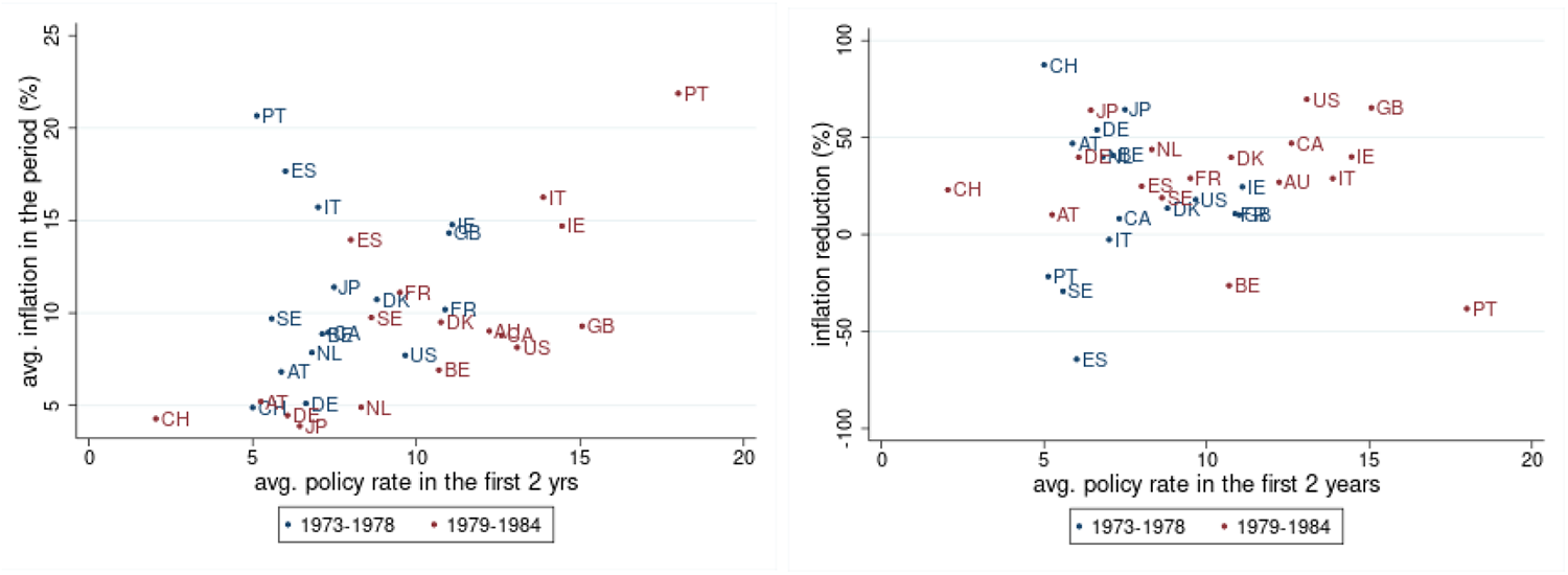
The cross-country heterogeneity in inflation performance detected in Section II can be generalized by examining a larger OECD sample. In Figure 8 we show the correlation between average policy rates in the first two years after each of the two oil shocks (horizontal axis) and two inflation outcomes, namely average inflation (left panel) and the percentage reduction in inflation (right panel) both recorded in the six years period after the two shocks. On average, a better inflation performance (lower average inflation or higher inflation reduction) does not appear to be systematically associated with the monetary policy response in terms of interest rates. In fact, particularly after the first shock, countries that initially maintained higher nominal interest rates (in line with higher inflation) generally experienced higher post-shock inflation and smaller subsequent reductions. After the second shock, amid increasingly restrictive monetary policies, we observe a mild association between policy rates and inflation reduction.
Average policy rates and inflation Note: Average policy rates are computed in the two years after the two oil shocks (x-axis); average inflation (left panel) and inflation reduction (right panel) are computed in the six years after the shocks. Inflation reduction is defined as the percentage difference in the average inflation levels between the first and the last two years of the period. Source: Our elaboration on BIS Statistics Warehouse, IMF/IFS and OECD.

This is merely a cross-country correlation and does not conclusively reflect the effectiveness of monetary policy. Nevertheless, it suggests that monetary conduct, as proxied by policy rates, does not fully explain cross-country differences in inflation, highlighting the need for further analysis of institutional and structural factors contributing to high inflation.
Insightfully, the governor of the Bank of Italy from 1979 to 1993, Carlo Azeglio Ciampi (Ciampi Reference Ciampi1981), argued that combating high and persistent inflation in Italy required the establishment of a ‘monetary constitution’, encompassing: (i) central bank independence; (ii) rules for sustainable and non-inflationary fiscal policy; (iii) labor market institutions. In this section, we discuss these three factors based on existing theoretical and empirical literature, and present some stylized facts on their correlation with inflation. As noted, the evidence presented consists of simple correlations, which cannot be interpreted as causal and are not conclusive.
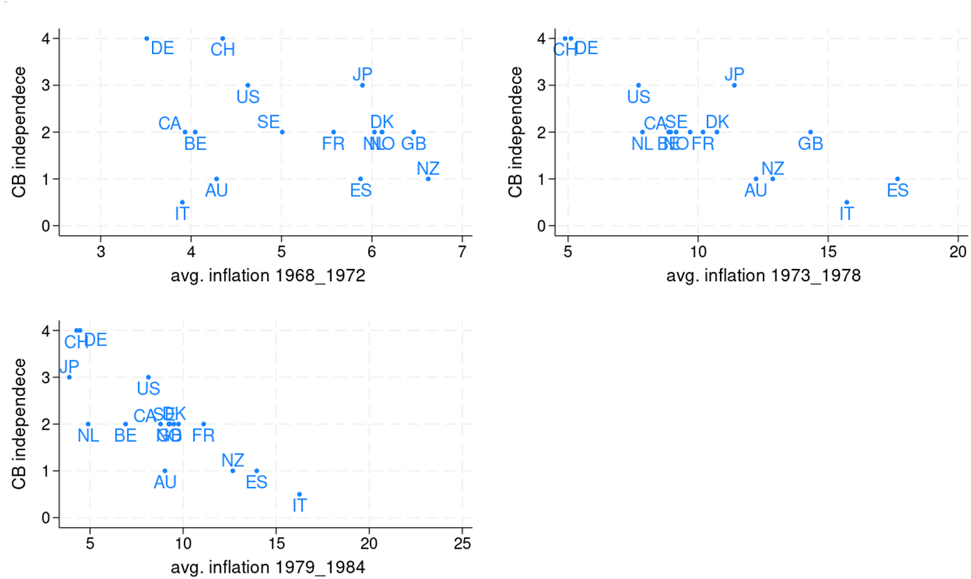
As discussed in the previous section, central bank independence was crucial in the development of a new monetary framework. In Figure 9, we plot the relationship between an index of central bank independence (from Alesina Reference Alesina1988Footnote 22) and average inflation before (upper left panel), after the first (upper right), and after the second oil shock (lower left). Central bank independence is strongly correlated with lower average inflation after both shocks. Notably, a negative association between independence and inflation emerges only from 1973, after the demise of the Bretton Woods monetary arrangements and the supply oil shocks, while these variables are uncorrelated beforehand.
Central bank degree of independence (y-axis) and average inflation (x-axis) Source: CBI index is from Alesina (Reference Alesina1988), average inflation is elaborated from BIS.

Regarding fiscal policy, expansionary policies were considered a major driver of inflation in the 1960s and 1970s. In Italy, for instance, public expenditure grew by approximately 11 percentage points of GDP during the 1970s, without a corresponding increase in taxation capacity (Salvati Reference Salvati, Lindberg and Maier1985). This was accompanied by the regulatory requirement for the central bank to purchase unsold public debt, at least until 1982. Central banks accumulated significant amounts of government debt (averaging 20 percent across advanced economies), which largely reflected the monetization of fiscal deficits (Eichengreen et al. Reference Eichengreen, El-Ganainy, Esteves and Mitchener2019). Bianchi and Melosi (Reference Bianchi and Melosi2022), making an explicit reference to the 1970s, argue that monetary tightening, in the presence of structural fiscal imbalances, is ineffective to curb medium and long-term inflation.
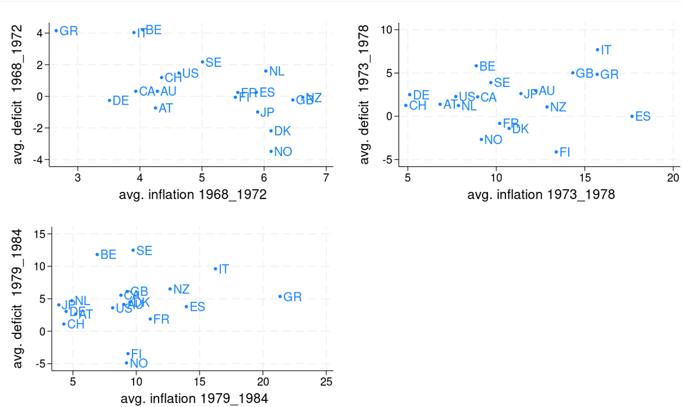
Looking at cross-country data, Figure 10 shows the correlation between the deficit-to-GDP ratio and inflation before and after the oil shocks (over a five-year period). While there is an overall positive association between the two variables after the shocks, the correlation is not clear-cut. For instance, Belgium had high deficits without above-average inflation, while countries like Spain and Finland experienced very high inflation despite having below-average deficits.Footnote 23
Average fiscal deficit to GDP (y-axis) and average inflation (x-axis) Source: Our elaboration on BIS Statistics Warehouse and IMF Historical Public Finance dataset (Mauro et al. Reference Mauro, Romeu, Binder and Zaman2013).

Finally, we examine labor market institutions, which can fuel second-round effects that may have been associated with cross-country differences in post-1973 inflation. We discuss three aspects, which are deeply intertwined: wage indexation, the degree of labor conflicts and the degree of wage-setting centralization.
First, the most straightforward and direct mechanism yielding nominal wage responsiveness to inflation is automatic wage indexation to price increases. In the Italian case, for example, the so-called ‘sliding-wage scale’, which implied a full adjustment of wages to price dynamics with a quarterly frequency, was regarded as one of the main culprits of inflation persistence in the 1970s and 1980s.Footnote 24
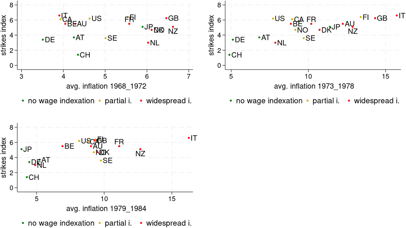
More generally, a high level of labor conflict, or ‘low cooperation’ in the labour market, has been identified as a source of inflationary pressures (Black Reference Black1982; McCallum Reference Mccallum1983). The rationale is that the high level of labor conflicts is expected to yield higher real wage rigidity to costs shocks.Footnote 25 Lorenzoni and Werning (Reference Lorenzoni and Werning2023) recently revived the case for conflict as the proximate cause of inflation. In Figure 11, we provide descriptive evidence on the cross-country association between labor conflicts, indexation and inflation. We plot the correlation between strike intensities on the y-axis (a proxy of conflictuality, as suggested by McCallum Reference Mccallum1983) and inflation on the x-axis, before and after the two oil shocks. The strike indexFootnote 26 is computed as an average over the 1950s and the 1960s, so it is predetermined with respect to the economic distress associated with the Great Inflation (which might have heightened labor conflicts). Furthermore, we classify countries according to the degree of wage indexation, that is classifying countries according to whether there is widespread indexation, partial or no indexation (associated to different colors in the graphs).Footnote 27 The scatter diagrams show that conflict and wage indexation are positively associated and are, in turn, both correlated to higher inflation after 1973.
Labor market conflicts (y-axis), wage indexation (colours) and average inflation (x-axis) Note: The strike index is the log of average annual working days lost per 1,000 non-agricultural employees, 1950–69. Source: for strike index, McCallum (Reference Mccallum1983); for wage indexation, Bruno and Sachs (Reference Bruno and Sachs1985).

A third element is the degree of centralization of wage setting at the national (or regional) level. Coupled with higher labor market cooperation, it was considered as another key labor market institutional aspect that played a structural role in the cross-country differential inflation patterns in the 1970s and 1980s. Bruno and Sachs (Reference Bruno and Sachs1985) and the Italian economist Tarantelli (Reference Tarantelli, Garonna, Mori and Tedeschi1992) claimed that labor markets in which wage setting was centralized and coordinated (which Tarantelli labeled neo-corporatist labor markets), widespread mostly in northern and continental Europe, fared better than decentralized labor market systems (such as those in the US, UK and ItalyFootnote 28), leading to a more favorable inflation–employment trade-off. The rationale goes as follows: centralized mechanisms, contrary to dispersed wage claims, determine a more efficient wage setting, allowing the internalization of the aggregate inflationary costs for workers. According to Tarantelli (Reference Tarantelli, Garonna, Mori and Tedeschi1992), a centralized wage-setting mechanism might curb inflation expectations through an ‘announcement effect’ in a similar fashion to monetary policy, although with smaller consequences in terms of output contractions. Such a scheme would require unions to be strong enough and willing to cooperate with both the government and the employers’ representatives, conceding on post-shock wage moderation in exchange for other outcomes (for instance, negotiating over labor income shares or welfare benefits).Footnote 29
In this respect, Hall (Reference Hall1994) exposes the case study of Germany, underlining that a cooperative and coordinated wage bargaining mechanism enhanced the effectiveness of central bank independence. Iversen (Reference Iversen1998) modeled the interaction between central bank independence and wage bargaining, showing that in intermediately centralized wage bargaining systems, restrictive monetary policies facilitate the solution of collective action problems by reducing the capacity for unions to externalize the costs of militancy. However, the benefits of wage bargaining centralization or coordination seems to be associated with the willingness of the unions to cooperate in a long-run timeframe. In this respect, Forteza (Reference Forteza1998) proves that non-inflationary equilibrium in wage bargaining rests on the assumption of ‘patient’ unions, i.e. having a sufficiently large discount factor of utility in future periods.
These arguments, that rest on unions to mitigate the coordination problem associated with wage inflation, may resonate in the opposite direction of the claim that nowadays lower workers’ bargaining power (proxied by unionization), compared to the 1970s, might be a sufficient reason to expect lower wage increases and therefore second-round effects (Boissay et al. Reference Boissay, De Fiore, Igan, Tejada and Rees2022; on the flattening of the Phillips curve related to the decline of workers’ bargaining power, see Lombardi, Riggi and Viviano Reference Lombardi, Riggi and Viviano2023). Empirically, in the 1970s a cross-country association between inflation and indexes of workers’ bargaining power does not emerge (Black Reference Black1982). This finding is plausibly influenced by two opposing effects: on the one hand, union power might have fostered higher wage claims; on the other side, in several countries higher union power fostered the capacity to build up more cooperative and farsighted labor market arrangements.
In a literature review, Flanagan (Reference Flanagan1999), maintains an overall empirical association between centralized bargaining systems and inflation in the 1970s and 1980s, but suggests caution in deriving clearcut policy implications, as these findings might be driven by several interdependent country-specific institutional features and time-specific conditions.
All in all, labor markets might play a significant role in inflation persistence to the extent that they untie wage dynamics from underlying productivity, chiefly, but not only, through automatic wage indexation to prices. The experience of the 1970s suggests that cooperative wage bargaining mechanisms, as far as they contributed to anchoring wage dynamics to underlying productivity, were helpful in containing inflation dynamics.
In the rest of this section we discuss how the institutional factors mentioned above have evolved since the 1970s across advanced economies. We acknowledge that these factors are multifaceted and assessing them synthetically and consistently over a large period is not straightforward. As far as we can, we rely on the available quantitative indexes that allow for consistent comparisons over time and across countries.
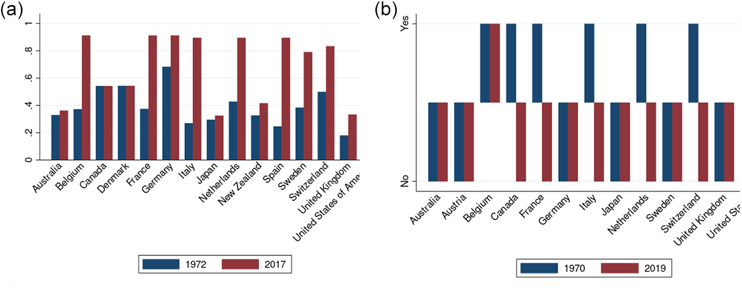
As is well known, central banks’ independence has increased over the decades in advanced economies with the aim to enhance anti-inflation credibility. This emerges also from a synthetic index in a new panel database provided by Romelli (Reference Romelli2022). The index is based on updating and enriching existing indexes of both political and economic independence. Notably, this work extends the country-specific time series up to 2017. In Figure 12, we show the indexes for 1972 and 2017 for several advanced economies. Almost all countries have seen a significant increase in central bank independence over time. That is driven to a large extent by the monetary integration of most European countries that share their monetary policy through the European Central Bank. However, even outside the Eurosystem, there is a clear positive trend in overall independence.
Institutional factors in OECD countries, then and now (a) Index of Central Bank Independence (b) Automatic wage indexation Source: (a) Romelli (Reference Romelli2022). The index builds on existing measurements of political and economic central bank independence, providing an expanded time-frame. It is ranged between 0 and 1. (b) OECD/AIAS ICTWSS database. Note: the variable takes value 1 (yes) if (most or many) collective agreements contain (semi-)automatic index or cost-of-living escalator; 0 (no) if use of index clauses is rare or forbidden.

As for the labour market, the degree of conflictuality, which was regarded as a driver of inflation persistence during the 1970s, is nowadays much less acute. Moreover, there is a widespread awareness of the unsustainability of automatic wage indexation mechanisms and their ineffectiveness as a tool to protect workers’ purchasing power in the longer term, at least as conceived in several countries in the 1970s. Such schemes are now relatively limited, as seen in results from the OECD/AIAS database (Visser Reference Visser2019), which uses a dummy variable to assess whether automatic wage indexation to consumer price clauses is significantly present in collective agreements (Figure 13). While these clauses were widespread in the early 1970s, they are now almost non-existent in advanced economies. The decline in wage indexation mitigates the risks of second-round effects materializing as in the past: a recent analysis has found that, before the 1990s, a large part of the inflationary effect of oil supply shocks in Europe was driven by second-round effects, fueled by wage and price setting behaviors (Battistini et al. Reference Battistini, Grapow, Hahn and Soudan2022).
Impulse response to oil price shock: Italy Note: The dashed line is the posterior median, while shaded bands correspond to the 68 per cent credible posterior region.

As for fiscal policies, we offer some brief remarks comparing the fiscal regimes of advanced economies now with those of 50 years ago. First, in the 1970s, many countries pursued expansionary fiscal policies that were not temporary measures tied to countercyclical considerations, but long-term oriented. These fiscal stances were allowed by larger possibilities to draw resources by monetary financing, a topic linked to the previously mentioned central bank independence. Second, such fiscal imbalances were mostly driven by current expenses rather than by public investments (Bordo, Bush and Thomas Reference Bordo, Bush and Thomas2022). The latter might have a less pronounced inflationary impact to the extent to which they foster an increase in potential output in the long run.Footnote 30 Overall, recent findings indicate a decrease in the inflationary impact of public deficits since the 1980s (International Monetary Fund 2023). This suggests that, under the current prevailing fiscal policy regimes, temporary and countercyclical expansionary fiscal policies, not being associated with expectations of long-term demand pressures, may have a smaller inflationary effect.
In the context of the European Union, countries signed the 2012 fiscal compact within the Treaty on Stability, Coordination and Governance in the Economic and Monetary Union, aimed at coordinating fiscal policies and ensuring their soundness. The effectiveness of this compact and the proposals for its reform have been and are a subject of debate and proposals of review. Tackling such a discussion is beyond the scope of this article. Nevertheless, it is worth noting that authoritative reform proposals, to the extent that they propose additional room for expansionary policies, typically allow it to pursue temporary countercyclical measures and/or in the form of larger public investments.Footnote 31
Overall, the picture of a more solid anti-inflationary institutional setting in the US emerges in the empirical analysis of Blanchard and Galí (Reference Blanchard, Galí, Galí and Gertler2009) and Blanchard and Riggi (Reference Blanchard and Riggi2013), who compare the impact of the oil shocks of the 1970s with those of the end of the 1990s and the early 2000s. The inflationary effects of oil price increases have diminished over time, largely due to three factors: the reduction in real wage rigidities; the increased credibility of monetary policy that lowered inflation expectations in response to oil shocks; and the reduced share of oil in consumption and production.
V
In this section, we conduct an econometric analysis aimed at measuring the impact of the oil shock and the relative contribution of the set of institutional factors and economic policies discussed in previous sections. To evaluate the macroeconomic effects of an oil shock, we estimate a Structural Vector Autoregression (SVAR) model that includes several variables that characterize the economy and the economic policies in place. Specifically, we build a medium-scale VAR specification at quarterly frequency, with seven variables: oil inflation, consumer inflation, GDP growth, nominal earning growth, exchange rate changes, policy rate, and the annual deficit over GDP.Footnote 32 The VAR is estimated using Bayesian methods with a quarterly sample running from 1960 to 1990 for three separate countries: Italy, Germany and the United States.
The VAR specification, with constant parameters, is the following:
 \begin{equation*}{y_t} = \mathop \sum \limits_{\ell = 1}^p {B_\ell } \cdot {y_{t - \ell }} + {u_t}, {u_t} \ {\textrm N}\left( {0,\Omega } \right).\end{equation*}
 To identify an exogenous oil shock we assume a simple triangular (Cholesky) decomposition of the covariance matrix ${\text{ }}\Omega $, where oil inflation is placed as the first variable. ${\text{ }}\Omega .$The corresponding SVAR representation of the model representing the orthogonal structural innovations ${\varepsilon _t}$ is:
 \begin{equation*}{{\text{A}}_0}{y_t} = \mathop \sum \limits_{\ell = 1}^p {A_\ell } \cdot {y_{t - \ell }} + {\varepsilon _t}.\end{equation*}
The main identifying assumption is that the oil inflation variable is the first variable, making structural innovations in the oil equation exogenous with respect to all other shocks. This identification approach follows Kilian (Reference Kilian2008) and Clark and Terry (Reference Clark and Terry2010).Footnote 33 Notably, the ordering of variables and the triangular identification scheme are agnostic about the response of macroecomic variables to the impact of the oil shock, allowing each variable to potentially react in any direction simultaneously.
Figure 13 plots the responses of the Italian economy to a one standard deviation shock in the rate of change of oil prices. The evidence suggests that an oil price shock triggers a large and persistent rise in inflation (lasting more than 20 quarters), along with a severe weakening in GDP dynamics in the first 10 quarters, before undertaking a gradual recovery, clearly resembling a strong and negative supply shock. The upward response of inflation is accompanied by a rise in earning inflation and a depreciation of the nominal exchange rate.Footnote 34 The responses depict a policy mix characterized by monetary tightening, suggested by a persistent increase in the policy rate, and a fiscal expansion, with the deficit-to-GDP ratio widening.
The same exercise for the US (Figure 14) reveals a similar pattern in the response of inflation, GDP and earning growth compared to Italy, although the response of the policy rate in the US shows a rise with a significant delay. The picture in Germany is markedly different (Figure 15): according to the VAR, while the oil shock induces a recession, it does not cause a persistent rise in consumer inflation, and earning inflation does not increase significantly. The interest rate reaction in Germany is also mild, most likely because the upward trend in interest rates had already begun before the oil crisis, in response to inflation and GDP overheating in the early 1970s.
Impulse response to oil price shock: US Note: The dashed line is the posterior median, while shaded bands correspond to the 68 percent credible posterior region.

Impulse response to oil price shock: Germany Note: The dashed line is the posterior median, while shaded bands correspond to the 68 per cent credible posterior region.

An alternative scheme relies on sign restrictions, which allow us to identify how variables respond to oil shocks upon impact. Using data for Italy and Germany, Figure 16 reports impulse response analyses with sign restrictions identifying the effects of an inflationary oil shock that contracts economic activity, depreciates the exchange rate and causes monetary policy to raise interest rates.Footnote 35 The results are very similar, both quantitatively and qualitatively, to those obtained under the benchmark Choleski specification.
Impulse response to oil price shock using sign restrictions: Italy and Germany Note: The dashed line is the posterior median, while shaded bands correspond to the 68 percent credible posterior region. The sign restrictions are detailed below.

Next, focusing on Italy we perform a counterfactual exercise, following Baumeister and Benati’s (Reference Baumeister and Benati2013) Zeroing Out strategy: we shut down the response of selected endogenous variables to the oil shock. This approach allows us to isolate the contribution of monetary policy, fiscal policy and earning dynamics to inflation persistence and GDP growth, conditioning on the large supply shock. In this exercise, we adopt the triangular identification scheme. Figure 17 shows the counterfactual response of some variables in Italy to the oil shock when the monetary policy response is zeroed-out: in this scenario, the GDP contraction would have been smaller and the recovery faster, but at the cost of much more persistent consumer and earnings inflation.
Zeroing out monetary policy: counterfactual response in Italy Note: The blue (dashed line) corresponds to the benchmark scenario, while the red (solid line) represents the counterfactual exercise where the response of the policy rate has been muted.

Figure 18 illustrates the counterfactual response to an oil shock if fiscal policy and earning inflation in Italy are zeroed out: the rise in consumer inflation would have been much less persistent, vanishing in a few years (less than 18 quarters). Similarly, the negative shock on GDP would have faded more quickly. Under these conditions, the policy rate could have been raised more moderately, reducing the extent of the monetary tightening that was implemented. In other words, fiscal policy and wage pressures to aggregate demand gave a crucial contribution to inflation persistence, making a huge monetary restriction necessary to control inflation. Absent these pressures, a much smaller policy response might have sufficed.Footnote 36
Zeroing out fiscal policy and earning inflation: counterfactual response in Italy Note: The blue (dashed line) corresponds to the benchmark scenario, while the red (solid line) represents the counterfactual exercise where the responses of earnings inflation and deficit/GDP have been zeroed out.

VI
This article presented a set of stylized facts related to the oil shocks that hit the world economy in the 1970s, triggering an inflation surge that proved highly persistent in some countries. By examining the cases of the US, Germany and Italy, we showed that the effects and the responses to the shocks were heterogeneous after the first shock in 1973 and more homogeneous after the second in 1979. Overall, the initial response of monetary policy is widely considered insufficient, failing to contain inflation in the 1970s. Consequently, a more severe monetary tightening was implemented following the second oil shock, contributing to economic slowdowns – or even recessions.
The initial ineffectiveness of monetary policy is closely tied to the end of the Bretton Woods era. The gold exchange standard, characterized by a fixed exchange rate regime and the currency peg to gold, collapsed in 1971 and resulted in the loss of a consolidated framework for monetary policy conduct. It took another two decades to establish a new framework centered on the commitment of independent and credible central banks to pursue explicit inflation targets.
In addition to the role played by monetary policy and by central bank independence, we showed that other institutional aspects played a pivotal role in explaining the diverse inflation outcomes across advanced economies. In particular, labor market characteristics – namely wage indexation and the low degree of cooperation in industrial relations – along with fiscal policy rules at odds with price stability, significantly contributed to inflation persistence. Using a structural VAR-based analysis we brought empirical evidence, in particular for Italy, on the contribution these factors gave to the sustained inflation experienced in the 1970s. A counterfactual exercise showed that inflation would have been considerably less persistent and the monetary policy response might have been milder, absent the pressure on price increases exerted by wage dynamics and fiscal policies.
Today, more credible and autonomous monetary policies, different mechanisms of wage indexation and negotiations, together with sustainable fiscal policies contribute to inflation not staying high for long.


 Open access