


1. Introduction
Magnetic reconnection is a phenomenon in which the topology of the magnetic field in a plasma is rearranged and magnetic energy is converted into kinetic or thermal energy (Yamada, Kulsrud & Ji Reference Yamada, Kulsrud and Ji2010; Ji et al. Reference Ji, Daughton, Jara-Almonte, Le, Stanier and Yoo2022). Reconnection has been widely observed and has broad applications in space plasma events, such as solar flares (Forbes Reference Forbes1991) and coronal mass ejections (Gosling, Birn & Hesse Reference Gosling, Birn and Hesse1995), the Earth’s and planetary magnetospheres (Chen et al. Reference Chen2008; Slavin et al. Reference Slavin2009; Le et al. Reference Le, Daughton, Chen and Egedal2017; Phan et al. Reference Phan2018; Hesse & Cassak Reference Hesse and Cassak2020), and in a wide variety of astrophysical and laboratory settings (Yamada et al. Reference Yamada, Levinton, Pomphrey, Budny, Manickam and Nagayama1994, Reference Yamada, Kulsrud and Ji2010; Uzdensky Reference Uzdensky2011; Hare et al. Reference Hare2018).
In the realm of collisionless reconnection, a persistent challenge has been to pinpoint the kinetic processes that facilitate rapid topological changes and energy conversion. Specifically, kinetic instabilities have been proposed to play an important role. These instabilities, through intense wave–particle interactions, may generate anomalous resistivity (Sagdeev Reference Sagdeev1967; Galeev & Sagdeev Reference Galeev and Sagdeev1983; Labelle & Treumann Reference Labelle and Treumann1988; Treumann Reference Treumann2014; Liu et al. Reference Liu, White, Francisquez, Milanese and Loureiro2024) and could determine the reconnection rate (Ji et al. Reference Ji, Yamada, Hsu and Kulsrud1998; Kulsrud Reference Kulsrud1998, Reference Kulsrud2014; Uzdensky Reference Uzdensky2003; Treumann Reference Treumann2014). Observational evidence (Carter et al. Reference Carter, Ji, Trintchouk, Yamada and Kulsrud2001; Deng & Matsumoto Reference Deng and Matsumoto2001; Farrell et al. Reference Farrell, Desch, Kaiser and Goetz2002; Matsumoto et al. Reference Matsumoto, Deng, Kojima and Anderson2003; Eastwood et al. Reference Eastwood, Phan, Bale and Tjulin2009; Laitinen et al. Reference Laitinen, Khotyaintsev, André, Vaivads and Rème2010; Graham et al. Reference Graham2017, Reference Graham2019; Khotyaintsev et al. Reference Khotyaintsev, Graham, Norgren and Vaivads2019; Chen et al. Reference Chen2020; Yoo et al. Reference Yoo2020; Wang et al. Reference Wang2022; Cozzani et al. Reference Cozzani, Khotyaintsev, Graham and André2023) and numerical simulations (Daughton Reference Daughton2003; Drake et al. Reference Drake, Swisdak, Cattell, Shay, Rogers and Zeiler2003; Daughton, Lapenta & Ricci Reference Daughton, Lapenta and Ricci2004; Roytershteyn et al. Reference Roytershteyn, Daughton, Karimabadi and Mozer2012; Fujimoto Reference Fujimoto2014; Jara-Almonte, Daughton & Ji Reference Jara-Almonte, Daughton and Ji2014; Le et al. Reference Le, Daughton, Ohia, Chen, Liu, Wang, Nystrom and Bird2018; Dokgo et al. Reference Dokgo, Hwang, Burch, Choi, Yoon, Sibeck and Graham2019; Le et al. Reference Le, Stanier, Daughton, Ng, Egedal, Nystrom and Bird2019; Ng et al. Reference Ng, Chen, Le, Stanier, Wang and Bessho2020a ; Wang et al. Reference Wang, Chen, Ng, Bessho and Hesse2021; Yi et al. Reference Yi, Pang, Song, Jin and Deng2023; Zhang et al. Reference Zhang2023) confirm the presence of turbulent phenomena and wave emissions in the vicinity of diffusion regions at reconnection sites, indicating that these instabilities are active players in reconnection dynamics. Moreover, they might affect the onset of reconnection itself (Ricci et al. Reference Ricci, Brackbill, Daughton and Lapenta2004; Alt & Kunz Reference Alt and Kunz2019; Winarto & Kunz Reference Winarto and Kunz2022).
Among the various potential kinetic modes, the ion-acoustic instability (IAI), driven by the relative drift between ions and electrons (or the electric current), has been proposed as a key factor in the dissipation of magnetic energy in collisionless plasmas (Coppi & Friedland Reference Coppi and Friedland1971; Smith & Priest Reference Smith and Priest1972; Coroniti & Eviatar Reference Coroniti and Eviatar1977; Sagdeev Reference Sagdeev1979) and appears to be a compelling explanation for numerous observations of ion-acoustic waves (IAWs) across different plasma settings. As far back as the 1970s, the Helios I and II missions have documented the presence of IAWs within heliocentric distances ranging from 0.3 to 1 AU (Gurnett & Anderson Reference Gurnett and Anderson1977; Gurnett & Frank Reference Gurnett and Frank1978), setting the stage for renewed interest in the role of these waves in the solar wind. More recently, advanced instrumentation from NASA’s Parker Solar Probe (PSP) (Fox et al. Reference Fox2015) and the European Space Agency’s Solar Orbiter (Müller et al. Reference Müller, Marsden, St. Cyr and Gilbert2012) has further highlighted the prominence of IAWs in the near-Sun environment. For example, the Solar Orbiter’s Time Domain Sampler receiver reveals that IAWs are a dominant wave mode close to the Sun (Graham et al. Reference Graham2021; Píša et al. Reference Píša2021), underscoring their importance for solar and heliospheric physics.
Observations of these waveforms may shed light on a longstanding question in solar physics: why proton temperatures in the solar wind decline much more slowly than predicted by simple adiabatic expansion, especially at distances beyond $20$
AU (Bridge et al. Reference Bridge, Belcher, Butler, Lazarus, Mavretic, Sullivan, Siscoe and Vasyliunas1977; Richardson & Smith Reference Richardson and Smith2003; Mozer et al. Reference Mozer, Agapitov, Kasper, Livi, Romeo and Vasko2023). This discrepancy implies the presence of additional heating mechanisms, possibly due to the turbulent nature of the solar wind (Tu & Marsch Reference Tu and Marsch1995; Bruno & Carbone Reference Bruno and Carbone2005). In particular, turbulence can drive localised magnetic reconnection events (Retinò et al. Reference Retinò, Sundkvist, Vaivads, Mozer, André and Owen2007; Servidio et al. Reference Servidio, Matthaeus, Shay, Cassak and Dmitruk2009, Reference Servidio, Dmitruk, Greco, Wan, Donato, Cassak, Shay, Carbone and Matthaeus2011; Osman et al. Reference Osman, Matthaeus, Gosling, Greco, Servidio, Hnat, Chapman and Phan2014; Loureiro & Boldyrev Reference Loureiro and Boldyrev2017) in the solar wind, with associated large currents. The existence of solar wind patches where ions are noticeably colder than electrons (Hellinger et al. Reference Hellinger, Trávníček, Štverák, Matteini and Velli2013; Štverák et al. Reference Štverák, Trávníček and Hellinger2015; Chen Reference Chen2016; Verscharen, Klein & Maruca Reference Verscharen, Klein and Maruca2019; Píša et al. Reference Píša2021) suggests that IAI can potentially be triggered in such events. Recent studies (Liu et al. Reference Liu, White, Francisquez, Milanese and Loureiro2024) and our own findings in this paper suggest that IAI can efficiently heat ions, providing a plausible explanation (among others) for the persistent, but not fully understood, ion heating in the solar wind over vast distances.
$20$
AU (Bridge et al. Reference Bridge, Belcher, Butler, Lazarus, Mavretic, Sullivan, Siscoe and Vasyliunas1977; Richardson & Smith Reference Richardson and Smith2003; Mozer et al. Reference Mozer, Agapitov, Kasper, Livi, Romeo and Vasko2023). This discrepancy implies the presence of additional heating mechanisms, possibly due to the turbulent nature of the solar wind (Tu & Marsch Reference Tu and Marsch1995; Bruno & Carbone Reference Bruno and Carbone2005). In particular, turbulence can drive localised magnetic reconnection events (Retinò et al. Reference Retinò, Sundkvist, Vaivads, Mozer, André and Owen2007; Servidio et al. Reference Servidio, Matthaeus, Shay, Cassak and Dmitruk2009, Reference Servidio, Dmitruk, Greco, Wan, Donato, Cassak, Shay, Carbone and Matthaeus2011; Osman et al. Reference Osman, Matthaeus, Gosling, Greco, Servidio, Hnat, Chapman and Phan2014; Loureiro & Boldyrev Reference Loureiro and Boldyrev2017) in the solar wind, with associated large currents. The existence of solar wind patches where ions are noticeably colder than electrons (Hellinger et al. Reference Hellinger, Trávníček, Štverák, Matteini and Velli2013; Štverák et al. Reference Štverák, Trávníček and Hellinger2015; Chen Reference Chen2016; Verscharen, Klein & Maruca Reference Verscharen, Klein and Maruca2019; Píša et al. Reference Píša2021) suggests that IAI can potentially be triggered in such events. Recent studies (Liu et al. Reference Liu, White, Francisquez, Milanese and Loureiro2024) and our own findings in this paper suggest that IAI can efficiently heat ions, providing a plausible explanation (among others) for the persistent, but not fully understood, ion heating in the solar wind over vast distances.
In this investigation, we focus specifically on the role of IAI in a simple, two-dimensional reconnecting configuration to determine whether it can provide a viable pathway for ion heating and wave generation within collisionless reconnection. Through a series of high-fidelity particle-in-cell numerical simulations, we find that this is indeed the case when the initial ion temperature is significantly lower than that of the electrons.
This paper is organised as follows. § 2 outlines the theoretical framework of IAI, highlighting its relevance to magnetic reconnection. § 3 describes the particle-in-cell simulation set-up and parameters. § 4 presents the results, including the reconnection rate (§ 4.1), conditions for IAI emergence (§ 4.2), evidence of IAW generation (§ 4.3) and the role of IAI in reconnection dynamics (§ 4.4). Finally, § 5 discusses the implications of these findings on ion heating in the solar wind and suggests directions for future research.
2. Theoretical framework
In this section, we revisit the IAI derivation by examining the wave mode solution parallel to the electron–ion drift. For non-relativistic systems, the Vlasov–Poisson equations are expressed as
 \begin{align} \frac {\partial f_{\alpha }}{\partial t} + \boldsymbol{v} \boldsymbol{\cdot }\boldsymbol{\nabla }f_{\alpha } & + \bigg (\!- \frac {q_{\alpha }}{m_{\alpha }} \boldsymbol{\nabla }\varphi \bigg ) \boldsymbol{\cdot }\frac {\partial f_{\alpha }}{\partial \boldsymbol{v}} = 0, \end{align}
 \begin{align} \boldsymbol{\nabla} ^2 \varphi &= -4\pi \sum _{\alpha } q_{\alpha } \int \text{d}^3 v\,f_{\alpha }, \end{align}
with $\alpha =i,e$
the particle species index. The combined and linearised equations for the
$\alpha =i,e$
the particle species index. The combined and linearised equations for the $1+1$
-dimensional
$1+1$
-dimensional $(x,v_x)$
case can be expressed in the form of a dielectric function
$(x,v_x)$
case can be expressed in the form of a dielectric function
 \begin{align} \epsilon (p, k) = 1 - \sum _{\alpha } \frac {\omega _{p\alpha }^2}{k^2} \frac {1}{n_{\alpha }} \int\, \text{d}v_x\,\frac {F^{\prime }_{\alpha } (v_x)}{v_x - ip/k}, \end{align}
where $\omega _{p\alpha }$
is the plasma frequency,
$\omega _{p\alpha }$
is the plasma frequency, $p \equiv -i\omega + \gamma$
and
$p \equiv -i\omega + \gamma$
and $F^{\prime }_{\alpha } (v_x)$
is the derivative of the one-dimensional (1-D) velocity distribution function with respect to
$F^{\prime }_{\alpha } (v_x)$
is the derivative of the one-dimensional (1-D) velocity distribution function with respect to $v_x$
. In the electrostatic scenario, the left-hand side of (2.3) is identically zero. By assuming both ion and electron species follow Maxwellian distributions, with electrons drifting at a speed
$v_x$
. In the electrostatic scenario, the left-hand side of (2.3) is identically zero. By assuming both ion and electron species follow Maxwellian distributions, with electrons drifting at a speed $U_d$
relative to the ions, (2.3) yields
$U_d$
relative to the ions, (2.3) yields
 \begin{align} 1 + \frac {1 + Z_p \big[({\omega - kU_d})/(\sqrt {2} k v_{\text{th},e})\big]}{k^2 \lambda _{De}^2} + \frac {1 + Z_p \big[{\omega }/(\sqrt {2} k v_{\text{th},i})\big]}{k^2 \lambda _{Di}^2} & \nonumber \\ + i \!\left \{ \frac {Z_{\varDelta } \big[({\omega - kU_d})/(\sqrt {2} k v_{\text{th},e})\big]}{k^2 \lambda _{De}^2} + \frac {Z_{\varDelta } \big[{\omega }/(\sqrt {2} k v_{\text{th},i})\big]}{k^2 \lambda _{Di}^2} \right \} &= 0, \end{align}
where $v_{\text{th},\alpha } = \sqrt {T_{\alpha }/m_{\alpha }}$
represents the thermal velocity,
$v_{\text{th},\alpha } = \sqrt {T_{\alpha }/m_{\alpha }}$
represents the thermal velocity, $\lambda _{D\alpha }$
the Debye length and we define
$\lambda _{D\alpha }$
the Debye length and we define
 \begin{align} Z_p (\zeta ) & \equiv - \text{erfi} (\zeta ) Z_{\varDelta } (\zeta ), \end{align}
 \begin{align} Z_{\varDelta } (\zeta ) & \equiv \sqrt {\pi } \zeta e^{-\zeta ^2}, \end{align}
and $\text{erfi} (\zeta )$
the imaginary error function. In the numerical simulations that follow, we find that both ions and electrons approximately follow (drifting) Maxwellian distributions within the diffusion region when IAI begins to be triggered, that is, when the peak outflow electron–ion drift starts to exceed the ion-acoustic threshold drift (see, e.g. figure 3). As such, the assumption of (drifting) Maxwellians employed in (2.4) is justified.
$\text{erfi} (\zeta )$
the imaginary error function. In the numerical simulations that follow, we find that both ions and electrons approximately follow (drifting) Maxwellian distributions within the diffusion region when IAI begins to be triggered, that is, when the peak outflow electron–ion drift starts to exceed the ion-acoustic threshold drift (see, e.g. figure 3). As such, the assumption of (drifting) Maxwellians employed in (2.4) is justified.
Equation (2.4) can be solved numerically to obtain the growth rates and spectrum of IAWs. Notably, IAI is only triggered under specific conditions. For $T_{i}/T_{e} \ll 1$
, a necessary criterion is that the electron–ion drift speed must be approximately or larger than the ion-sound speed
$T_{i}/T_{e} \ll 1$
, a necessary criterion is that the electron–ion drift speed must be approximately or larger than the ion-sound speed $c_s = \sqrt {(\gamma _e T_e + \gamma _i T_i)/m_i} \approx \sqrt {(T_e + 3 T_i)/m_i}$
,Footnote
1
where
$c_s = \sqrt {(\gamma _e T_e + \gamma _i T_i)/m_i} \approx \sqrt {(T_e + 3 T_i)/m_i}$
,Footnote
1
where $\gamma _{\alpha }$
is the adiabatic index of species
$\gamma _{\alpha }$
is the adiabatic index of species $\alpha$
, and we have assumed that electrons are isothermal (
$\alpha$
, and we have assumed that electrons are isothermal ( $\gamma _{e} = 1$
) and ions are adiabatic (
$\gamma _{e} = 1$
) and ions are adiabatic ( $\gamma _{i} = 3$
) (Biskamp Reference Biskamp2000).
$\gamma _{i} = 3$
) (Biskamp Reference Biskamp2000).
In the context of collisionless magnetic reconnection, one may expect IAI to be driven in both the out-of-plane and in-plane directions. The out-of-plane direction is influenced by the reconnection current and the associated reconnection electric field, while the in-plane direction is driven by the current and electric field resulting from decoupled ion and electron flows in the outflow direction. The former mechanism was briefly addressed by Liu et al. (Reference Liu, White, Francisquez, Milanese and Loureiro2024). The condition for the onset of out-of-plane IAI can be approximated as
 \begin{align} \frac {J_z/en}{c_s} \sim \frac {cB_0}{4\pi \delta en} \sqrt {\frac {m_i}{T_e}} = \sqrt {\frac {2}{\beta _e}} \frac {d_i}{\delta } \gt 1, \end{align}
where $J_z$
is the out-of-plane current density,
$J_z$
is the out-of-plane current density, $B_0$
is the upstream (reconnecting) magnetic field,
$B_0$
is the upstream (reconnecting) magnetic field, $\delta$
is the current sheet thickness,
$\delta$
is the current sheet thickness, $d_{i} = c/\omega _{pi} = c (m_i/4\pi n e^2)^{1/2}$
is the ion inertial length or ion skin-depth and
$d_{i} = c/\omega _{pi} = c (m_i/4\pi n e^2)^{1/2}$
is the ion inertial length or ion skin-depth and $\beta _e$
is the electron plasma beta based on the reconnecting field. This condition is easy to satisfy since
$\beta _e$
is the electron plasma beta based on the reconnecting field. This condition is easy to satisfy since $\delta$
is expected to be of the order of the electron skin-depth.
$\delta$
is expected to be of the order of the electron skin-depth.
Likewise, it is inevitable that the in-plane IAI will be triggered if $T_i/T_e \ll 1$
because the in-plane electron–ion drift should reach
$T_i/T_e \ll 1$
because the in-plane electron–ion drift should reach $U_{d,\text{in-plane}} \simeq v_{A,e} - v_{A,i}$
, giving
$U_{d,\text{in-plane}} \simeq v_{A,e} - v_{A,i}$
, giving
 \begin{align} \frac {U_{d,\text{in-plane}}}{c_s} \sim \frac {v_{A,e} - v_{A,i}}{c_s} \simeq \frac {v_{A,e}}{c_s} = \frac {B_0}{\sqrt {4\pi n_e m_e}} \sqrt {\frac {m_i}{T_e}} = \sqrt {\frac {m_i}{m_e}} \sqrt {\frac {2}{\beta _e}} \gg 1, \end{align}
where $v_{A,\alpha } = B_0/(4\pi n_{\alpha } m_{\alpha })^{1/2}$
is the Alfvén speed of species
$v_{A,\alpha } = B_0/(4\pi n_{\alpha } m_{\alpha })^{1/2}$
is the Alfvén speed of species $\alpha$
. This result is illustrated in figure 1, which presents numerical solutions of the growth rate for the fastest growing wave mode and the wavenumber at which this maximum growth rate occurs, calculated by solving (2.4) using the initial thermal velocities from the simulations that follow and assuming uniform number densities
$\alpha$
. This result is illustrated in figure 1, which presents numerical solutions of the growth rate for the fastest growing wave mode and the wavenumber at which this maximum growth rate occurs, calculated by solving (2.4) using the initial thermal velocities from the simulations that follow and assuming uniform number densities $n_i = n_e = n_b = 0.2 n_0$
(the approximate ion and electron density near the x-point around the time of peak reconnection rate in all simulations). The figure shows that there exists a range of drift speeds below the theoretical maximum of
$n_i = n_e = n_b = 0.2 n_0$
(the approximate ion and electron density near the x-point around the time of peak reconnection rate in all simulations). The figure shows that there exists a range of drift speeds below the theoretical maximum of $U_d = v_{A,e} - v_{A,i}$
(identified by the purple vertical lines in figure 1
Footnote
2
) for which the growth rate of the fastest growing mode is positive for all ion–electron temperature ratios considered. In the numerical simulations that follow, we find that the outflow electron–ion drift speed
$U_d = v_{A,e} - v_{A,i}$
(identified by the purple vertical lines in figure 1
Footnote
2
) for which the growth rate of the fastest growing mode is positive for all ion–electron temperature ratios considered. In the numerical simulations that follow, we find that the outflow electron–ion drift speed $|U_{d,\text{outflow}}| = |u_{x,e} - u_{xi}|$
reaches
$|U_{d,\text{outflow}}| = |u_{x,e} - u_{xi}|$
reaches $\approx v_{A,e}/2$
at the outflow ends of the diffusion region, a result that is roughly independent of temperature ratio (see figures 4 and 3), which, alongside figure 1, suggests that IAI can be strongly triggered for
$\approx v_{A,e}/2$
at the outflow ends of the diffusion region, a result that is roughly independent of temperature ratio (see figures 4 and 3), which, alongside figure 1, suggests that IAI can be strongly triggered for $T_{i0}/T_{e0} = 1/10$
and
$T_{i0}/T_{e0} = 1/10$
and $1/50$
, but not for
$1/50$
, but not for $T_{i0}/T_{e0} = 1$
.
$T_{i0}/T_{e0} = 1$
.
Due to computational constraints, this study considers only the two-dimensional case, with the out-of-plane and invariant direction aligned with $\hat {\boldsymbol{z}}$
, and focuses exclusively on the in-plane component of IAI.
$\hat {\boldsymbol{z}}$
, and focuses exclusively on the in-plane component of IAI.
Maximum growth rates ( $\gamma _{\text{max}}$
, in blue) and the corresponding wavenumbers (
$\gamma _{\text{max}}$
, in blue) and the corresponding wavenumbers ( $k_{\text{max}}$
, in orange) as functions of drift velocity (
$k_{\text{max}}$
, in orange) as functions of drift velocity ( $U_d$
) for
$U_d$
) for $T_{i0}/T_{e0} = 1$
(dotted lines),
$T_{i0}/T_{e0} = 1$
(dotted lines), $T_{i0}/T_{e0} = 1/10$
(dashed lines) and
$T_{i0}/T_{e0} = 1/10$
(dashed lines) and $T_{i0}/T_{e0} = 1/50$
(solid lines). These values are obtained from solving (2.4), using the thermal velocities initialised in the simulations and
$T_{i0}/T_{e0} = 1/50$
(solid lines). These values are obtained from solving (2.4), using the thermal velocities initialised in the simulations and $n_i = n_e = n_b = 0.2 n_0$
. Regions not accessible within the considered reconnection configuration along the outflow symmetry line are shaded in purple, with the purple lines representing the maximum expected electron–ion drift velocity (
$n_i = n_e = n_b = 0.2 n_0$
. Regions not accessible within the considered reconnection configuration along the outflow symmetry line are shaded in purple, with the purple lines representing the maximum expected electron–ion drift velocity ( $U_{d,\text{in-plane}} = v_{A,e} - v_{A,i}$
) at the ends of the diffusion region for each ion–electron temperature ratio. The increase in
$U_{d,\text{in-plane}} = v_{A,e} - v_{A,i}$
) at the ends of the diffusion region for each ion–electron temperature ratio. The increase in $k_{\text{max}}$
at
$k_{\text{max}}$
at $\gamma _{\text{max}} = 0$
as
$\gamma _{\text{max}} = 0$
as $T_{i0}/T_{e0}$
decreases beyond
$T_{i0}/T_{e0}$
decreases beyond $1/10$
is explained in Appendix A.
$1/10$
is explained in Appendix A.

3. Simulation set-up
The simulations reported in this work are conducted using the particle-in-cell (PIC) code osiris (Fonseca et al. Reference Fonseca2002; Hemker Reference Hemker2015). The initial conditions are set to a Harris sheet equilibrium (Harris Reference Harris1962), with the initial magnetic vector potential expressed as
 \begin{eqnarray} \boldsymbol{A} = \hat {\boldsymbol{z}} B_0 \lambda _{\text{B}} \ln \bigg [ \cosh \bigg ( \frac {y}{\lambda _{\text{B}}} \bigg ) \bigg ]. \end{eqnarray}
Here, $\lambda _{\text{B}}$
is the characteristic length scale of the magnetic field gradient (half-width of the current sheet). The initial density distribution is defined as
$\lambda _{\text{B}}$
is the characteristic length scale of the magnetic field gradient (half-width of the current sheet). The initial density distribution is defined as
 \begin{eqnarray} n_e = n_i = n_0 \text{sech}^2 \bigg ( \frac {y}{\lambda _{\text{B}}} \bigg ) + n_b, \end{eqnarray}
with $n_b = 0.2n_0$
the background number density.
$n_b = 0.2n_0$
the background number density.
The global Alfvén time is defined as $t_A = L_x/v_{A,i0}$
, where
$t_A = L_x/v_{A,i0}$
, where $L_x$
and
$L_x$
and $L_y$
are the lengths of the simulation box in the
$L_y$
are the lengths of the simulation box in the $x$
(outflow) and
$x$
(outflow) and $y$
(inflow) directions. The ion and electron out-of-plane current densities are specified by
$y$
(inflow) directions. The ion and electron out-of-plane current densities are specified by $J_{zi0}/J_{ze0} = T_{i0}/T_{e0}$
to establish Vlasov equilibrium (Schindler Reference Schindler2006), with
$J_{zi0}/J_{ze0} = T_{i0}/T_{e0}$
to establish Vlasov equilibrium (Schindler Reference Schindler2006), with $T_{i0}$
and
$T_{i0}$
and $T_{e0}$
uniform, and
$T_{e0}$
uniform, and $\boldsymbol{J}_0 = c(\boldsymbol{\nabla }\times \boldsymbol{B}_0/4\pi )$
. The force-balance condition is satisfied by setting
$\boldsymbol{J}_0 = c(\boldsymbol{\nabla }\times \boldsymbol{B}_0/4\pi )$
. The force-balance condition is satisfied by setting $n_0 (T_{i0} + T_{e0}) = B_0^2/8\pi$
. The relationship between the electron plasma and cyclotron frequencies is given by
$n_0 (T_{i0} + T_{e0}) = B_0^2/8\pi$
. The relationship between the electron plasma and cyclotron frequencies is given by $\omega _{pe} = 2\varOmega _{ce}$
, where
$\omega _{pe} = 2\varOmega _{ce}$
, where $\omega _{pe} = (4\pi n_0 e^2/m_e)^{1/2}$
and
$\omega _{pe} = (4\pi n_0 e^2/m_e)^{1/2}$
and $\varOmega _{ce} = |e|B_0/(m_e c)$
.
$\varOmega _{ce} = |e|B_0/(m_e c)$
.
The initial perturbation is similar to that described by Daughton et al. (Reference Daughton, Roytershteyn, Albright, Karimabadi, Yin and Bowers2009), with $\delta \boldsymbol{B} = \hat {\boldsymbol{z}} \times \boldsymbol{\nabla }\psi$
and
$\delta \boldsymbol{B} = \hat {\boldsymbol{z}} \times \boldsymbol{\nabla }\psi$
and $\psi = - \delta \psi \cos (2\pi x/L_x) \cos (\pi y/L_y)$
, where the perturbation amplitude is set to
$\psi = - \delta \psi \cos (2\pi x/L_x) \cos (\pi y/L_y)$
, where the perturbation amplitude is set to $\delta \psi /B_0 d_{i0} = 0.1$
. We use cubic particle interpolations and resolve the electron Debye length (
$\delta \psi /B_0 d_{i0} = 0.1$
. We use cubic particle interpolations and resolve the electron Debye length ( $\lambda _{De}$
) to prevent numerical heating. As a result, it was essential to adjust the resolution and time step parameters based on the ion–electron temperature ratio.
$\lambda _{De}$
) to prevent numerical heating. As a result, it was essential to adjust the resolution and time step parameters based on the ion–electron temperature ratio.
Key simulation parameters used in these runs are listed in tables 1 and 2.
Summary of simulation parameters.

Simulation-specific parameters.

4. Simulation results and wave activity in the diffusion region
In this section, we describe and analyse in detail the results of our numerical simulations. We begin with an overview of the reconnection dynamics observed across the simulations, emphasising the relatively minor impact of the temperature ratio on the reconnection rate. Despite this, significant wave activity is detected in the diffusion region, leading to pronounced ion heating. We argue in the following sections that this wave activity is driven by IAI, and characterise its onset and impact on reconnection dynamics.
4.1. Reconnection rate
Plotted in figure 2 is the normalised reconnection rate (computed as the difference in the magnetic vector potential’s rate of change at the X and O points, and temporally averaged over a moving window of ${\approx} 0.03\,t_A$
) for each value of the ion–electron temperature ratio that we have numerically simulated. As shown, we find that the onset of fast reconnection occurs earlier in time for colder ions; however, the peak reconnection rate is weakly dependent on the temperature ratio – varying by less than a factor of 2 across values of
${\approx} 0.03\,t_A$
) for each value of the ion–electron temperature ratio that we have numerically simulated. As shown, we find that the onset of fast reconnection occurs earlier in time for colder ions; however, the peak reconnection rate is weakly dependent on the temperature ratio – varying by less than a factor of 2 across values of $T_{i0}/T_{e0}$
ranging from
$T_{i0}/T_{e0}$
ranging from $1/50$
to
$1/50$
to $1$
– and is consistent with the established values in the literature (e.g. Birn et al. Reference Birn2001; Cassak, Liu & Shay Reference Cassak, Liu and Shay2017). Also evident from the plot is the highly oscillatory nature of the curves corresponding to low initial temperature ratios during the fast reconnection stage, in contrast with the
$1$
– and is consistent with the established values in the literature (e.g. Birn et al. Reference Birn2001; Cassak, Liu & Shay Reference Cassak, Liu and Shay2017). Also evident from the plot is the highly oscillatory nature of the curves corresponding to low initial temperature ratios during the fast reconnection stage, in contrast with the $T_{i0}/T_{e0}=1$
case. This behaviour hints at turbulent dynamics in the current sheet during those times which, as we will demonstrate later, is due to the destabilisation of ion-acoustic modes.
$T_{i0}/T_{e0}=1$
case. This behaviour hints at turbulent dynamics in the current sheet during those times which, as we will demonstrate later, is due to the destabilisation of ion-acoustic modes.
Time evolution of the temporally averaged reconnection rate for $T_{i0}/T_{e0} = 1/50$
(blue),
$T_{i0}/T_{e0} = 1/50$
(blue), $T_{i0}/T_{e0} = 1/10$
(orange) and
$T_{i0}/T_{e0} = 1/10$
(orange) and $T_{i0}/T_{e0} = 1$
(purple).
$T_{i0}/T_{e0} = 1$
(purple). $A_{zX}$
and
$A_{zX}$
and $A_{zO}$
are the out-of-plane magnetic vector potentials at the X and O points, respectively, and the semi-transparent curves are more exact values of the solid curves.
$A_{zO}$
are the out-of-plane magnetic vector potentials at the X and O points, respectively, and the semi-transparent curves are more exact values of the solid curves.

4.2. Onset of ion acoustic instability (IAI)
We find that the outflow electron–ion drift speed $|U_{d,\text{outflow}}|$
exceeds the IAI threshold drift in the diffusion region and near the separatrix for the cases
$|U_{d,\text{outflow}}|$
exceeds the IAI threshold drift in the diffusion region and near the separatrix for the cases $T_{i0}/T_{e0}=1/50$
and
$T_{i0}/T_{e0}=1/50$
and $1/10$
. This is shown in figure 3, which illustrates the evolution of the outflow electron–ion drift along the outflow symmetry line (
$1/10$
. This is shown in figure 3, which illustrates the evolution of the outflow electron–ion drift along the outflow symmetry line ( $y = 0$
) near the x-point for the different temperature ratios considered, compared with the corresponding IAI threshold drift speeds (dashed lines; at times when the peak drifts begin to exceed the thresholds), calculated with local ion-acoustic speeds
$y = 0$
) near the x-point for the different temperature ratios considered, compared with the corresponding IAI threshold drift speeds (dashed lines; at times when the peak drifts begin to exceed the thresholds), calculated with local ion-acoustic speeds $c_s = \sqrt {(T_{e,xx} + 3 T_{i,xx})/m_i}$
. This drift occurs within the ion diffusion region because ions decouple from the magnetic field lines on electron scales, allowing for both ion and electron outflow speeds to approach their respective Alfvén speeds (Shay & Drake Reference Shay and Drake1998; Liu et al. Reference Liu, Cassak, Li, Hesse, Lin and Genestreti2022).
$c_s = \sqrt {(T_{e,xx} + 3 T_{i,xx})/m_i}$
. This drift occurs within the ion diffusion region because ions decouple from the magnetic field lines on electron scales, allowing for both ion and electron outflow speeds to approach their respective Alfvén speeds (Shay & Drake Reference Shay and Drake1998; Liu et al. Reference Liu, Cassak, Li, Hesse, Lin and Genestreti2022).
Evolution of the outflow electron–ion drift ( $U_d = u_{x,e} - u_{x,i}$
), normalised to the initial electron thermal velocity
$U_d = u_{x,e} - u_{x,i}$
), normalised to the initial electron thermal velocity $u_{\text{th},e}$
, along the outflow symmetry line (
$u_{\text{th},e}$
, along the outflow symmetry line ( $y = 0$
) for (a)
$y = 0$
) for (a) $T_{i0}/T_{e0} = 1$
, (b)
$T_{i0}/T_{e0} = 1$
, (b) $T_{i0}/T_{e0} = 1/10$
and (c)
$T_{i0}/T_{e0} = 1/10$
and (c) $T_{i0}/T_{e0} = 1/50$
. The blue curves denote the times when the drifts begin to exceed the corresponding IAI thresholds (which, for
$T_{i0}/T_{e0} = 1/50$
. The blue curves denote the times when the drifts begin to exceed the corresponding IAI thresholds (which, for $T_{i0}/T_{e0} = 1$
, never occurs and thus no blue curve is shown in panel a), the purple curves refer to the approximate times of peak reconnection rates and the red curves represent later times when the drifts reach maximum values. Dashed lines show the corresponding IAI threshold drift speeds (at times when the peak drifts begin to exceed the thresholds), calculated with local ion-acoustic speeds
$T_{i0}/T_{e0} = 1$
, never occurs and thus no blue curve is shown in panel a), the purple curves refer to the approximate times of peak reconnection rates and the red curves represent later times when the drifts reach maximum values. Dashed lines show the corresponding IAI threshold drift speeds (at times when the peak drifts begin to exceed the thresholds), calculated with local ion-acoustic speeds $c_s = \sqrt {(T_{e,xx} + 3 T_{i,xx})/m_i}$
.
$c_s = \sqrt {(T_{e,xx} + 3 T_{i,xx})/m_i}$
.

The separation of electron and ion outflow velocities is illustrated in the phase-space distributions presented in figure 4 (see also figure 3 and the contours in figure 5), which shows ion and electron phase-space densities as functions of the particles’ proper velocity and position in the outflow direction ( $u_x$
and
$u_x$
and $x$
, respectively). Figure 4(a,b) also reveals nonlinear ion phase-space structures, which coincide with the emergence of waveforms in the diffusion region that, in the next subsection, we associate with IAWs.
$x$
, respectively). Figure 4(a,b) also reveals nonlinear ion phase-space structures, which coincide with the emergence of waveforms in the diffusion region that, in the next subsection, we associate with IAWs.
Notably, figure 4 demonstrates that the maximum ion proper velocities (which are approximately ion bulk velocities due to the relatively low ion temperatures), attained at the end-points of the current sheet, closely match the Alfvén speed at those locations ( $v_{A,i} \simeq 0.15 u_{\text{th,e}}$
), aligning with the established understanding of reconnection physics that the bulk plasma is accelerated to
$v_{A,i} \simeq 0.15 u_{\text{th,e}}$
), aligning with the established understanding of reconnection physics that the bulk plasma is accelerated to $v_{A,i}$
in the outflow direction. The maximum electron outflow velocity, which is
$v_{A,i}$
in the outflow direction. The maximum electron outflow velocity, which is ${\approx} 0.8 u_{\text{th,e}} \approx v_{A,e}/2$
(see figure 3), being much larger than that of the ions implies that there is a large in-plane current.Footnote
3
${\approx} 0.8 u_{\text{th,e}} \approx v_{A,e}/2$
(see figure 3), being much larger than that of the ions implies that there is a large in-plane current.Footnote
3
(a,b) Ion and (c,d) electron phase-space distributions in $u_x$
and
$u_x$
and $x$
along the outflow symmetry line (
$x$
along the outflow symmetry line ( $y = 0$
) near the x-point for (a,c)
$y = 0$
) near the x-point for (a,c) $T_{i0}/T_{e0} = 1/10$
and (b,d)
$T_{i0}/T_{e0} = 1/10$
and (b,d) $T_{i0}/T_{e0} = 1/50$
at the approximate times when IAI is strongly triggered.
$T_{i0}/T_{e0} = 1/50$
at the approximate times when IAI is strongly triggered.

Figure 3 shows that that the electron–ion drifts begin to exceed the corresponding IAI thresholds (see figure 1, which gives $U_{d,\text{IAI}}/c_s = U_d \ (\gamma _{\text{max}} = 0)/c_s \approx 7.19$
,
$U_{d,\text{IAI}}/c_s = U_d \ (\gamma _{\text{max}} = 0)/c_s \approx 7.19$
, $1.36$
and
$1.36$
and $0.68$
for
$0.68$
for $T_{i0}/T_{e0} = 1$
,
$T_{i0}/T_{e0} = 1$
, $1/10$
and
$1/10$
and $1/50$
) at
$1/50$
) at $t \approx 0.74\,t_A$
and
$t \approx 0.74\,t_A$
and $t \approx 0.59\,t_A$
for
$t \approx 0.59\,t_A$
for $T_{i0}/T_{e0} = 1/10$
and
$T_{i0}/T_{e0} = 1/10$
and $1/50$
, respectively. These approximate times correlate well with the emergence of waveforms in the diffusion region (see figure 6 for the
$1/50$
, respectively. These approximate times correlate well with the emergence of waveforms in the diffusion region (see figure 6 for the $T_{i0}/T_{e0} = 1/50$
case).
$T_{i0}/T_{e0} = 1/50$
case).
We further demonstrate the decoupling between electron and ion drifts in figure 5, which displays colourmaps of the outflow electron–ion drift velocity along with contours highlighting where this drift exceeds the associated IAI threshold drift. Additionally, it depicts the magnitude of the outflow electric field ( $E_x$
), whose wave-like structures we examine in detail in the next section.
$E_x$
), whose wave-like structures we examine in detail in the next section.
Colourmap displaying the $x$
-component of the electron–ion drift velocity normalised to the IAI threshold drifts, calculated with local ion-acoustic speeds
$x$
-component of the electron–ion drift velocity normalised to the IAI threshold drifts, calculated with local ion-acoustic speeds $c_s = \sqrt {(T_{e,xx} + 3 T_{i,xx})/m_i}$
(red-blue), overlaid with contours indicating the regions where
$c_s = \sqrt {(T_{e,xx} + 3 T_{i,xx})/m_i}$
(red-blue), overlaid with contours indicating the regions where $|u_{x,e} - u_{x,i}|/U_{d,\text{IAI}} \simeq 1$
(magenta) and the magnitude of the outflow electric field (
$|u_{x,e} - u_{x,i}|/U_{d,\text{IAI}} \simeq 1$
(magenta) and the magnitude of the outflow electric field ( $E_x$
, normalised to the reference value
$E_x$
, normalised to the reference value $E_0 = m_e c \omega _{pe}/e$
and in grey scale) shortly after the time of maximum reconnection rate (see figure 2). This is shown for the following cases: (a,d)
$E_0 = m_e c \omega _{pe}/e$
and in grey scale) shortly after the time of maximum reconnection rate (see figure 2). This is shown for the following cases: (a,d) $T_{i0}/T_{e0} = 1$
; (b,e)
$T_{i0}/T_{e0} = 1$
; (b,e) $T_{i0}/T_{e0} = 1/10$
and (c,f)
$T_{i0}/T_{e0} = 1/10$
and (c,f) $T_{i0}/T_{e0} = 1/50$
. Panels (d)–(f) zoom in on the diffusion region, as identified by the boxes in panels (a)–(c).
$T_{i0}/T_{e0} = 1/50$
. Panels (d)–(f) zoom in on the diffusion region, as identified by the boxes in panels (a)–(c).

4.3. Identification of IAWs
A salient feature in the contour plots of figure 5 is the appearance of wave-like structures in the diffusion region, particularly for the cases where $T_{i0}/T_{e0} = 1/10$
and
$T_{i0}/T_{e0} = 1/10$
and $1/50$
. These structures suggest the presence of underlying kinetic instabilities, likely associated with IAWs. To better understand the origin of this wave activity, we now focus on a detailed analysis of the diffusion region.
$1/50$
. These structures suggest the presence of underlying kinetic instabilities, likely associated with IAWs. To better understand the origin of this wave activity, we now focus on a detailed analysis of the diffusion region.
To isolate the waveforms specifically associated with the instability, we concentrate on the outflow electric field, $E_x$
. This approach helps to avoid interference from background electromagnetic field structures, as the baseline outflow electric field is much weaker than the observed fluctuations. As a result, any detected
$E_x$
. This approach helps to avoid interference from background electromagnetic field structures, as the baseline outflow electric field is much weaker than the observed fluctuations. As a result, any detected $E_x$
perturbations can be directly attributed to wave activity. Figure 5 highlights the regions where large-amplitude waveforms of the outflow electric field are concentrated, indicating that these waves are generated and confined in regions where the outflow electron–ion drift velocity significantly exceeds the IAI threshold drift. These observations, combined with the absence of significant wave activity in the
$E_x$
perturbations can be directly attributed to wave activity. Figure 5 highlights the regions where large-amplitude waveforms of the outflow electric field are concentrated, indicating that these waves are generated and confined in regions where the outflow electron–ion drift velocity significantly exceeds the IAI threshold drift. These observations, combined with the absence of significant wave activity in the $T_{i0}/T_{e0} = 1$
case, strongly suggest that the waveforms are generated by IAI, triggered by the large outflow current.
$T_{i0}/T_{e0} = 1$
case, strongly suggest that the waveforms are generated by IAI, triggered by the large outflow current.
The evolution of these waveforms for $T_{i0}/T_{e0} = 1/50$
is depicted in figure 6(a,b), showing the outflow electric field near the x-point along the outflow symmetry line (
$T_{i0}/T_{e0} = 1/50$
is depicted in figure 6(a,b), showing the outflow electric field near the x-point along the outflow symmetry line ( $y = 0$
) as a function of
$y = 0$
) as a function of $x$
and
$x$
and $t$
. By performing two-dimensional Fourier transforms, we obtain spectra of the outflow electric field near the x-point, shown in figure 6(c,d). These spectra are compared with the solutions to the linearised Vlasov–Poisson equation (2.4), first assuming zero ion drift (in the lab frame) to obtain
$t$
. By performing two-dimensional Fourier transforms, we obtain spectra of the outflow electric field near the x-point, shown in figure 6(c,d). These spectra are compared with the solutions to the linearised Vlasov–Poisson equation (2.4), first assuming zero ion drift (in the lab frame) to obtain $\omega _{\text{Vlasov}} (k)$
(shown as the blue dashed line) and then Doppler-shifted by the maximum ion outflow drift at the outflow ends of the current sheet (red dashed line; we find that
$\omega _{\text{Vlasov}} (k)$
(shown as the blue dashed line) and then Doppler-shifted by the maximum ion outflow drift at the outflow ends of the current sheet (red dashed line; we find that $u_{x,i}$
reaches
$u_{x,i}$
reaches $u_{x,i, \text{max}} \simeq 0.8 v_{A,i0}$
along the outflow symmetry line before IAI saturates and the current sheet becomes strongly nonlinear). The Doppler-shifted solution to the linearised Vlasov–Poisson equations is calculated as simply
$u_{x,i, \text{max}} \simeq 0.8 v_{A,i0}$
along the outflow symmetry line before IAI saturates and the current sheet becomes strongly nonlinear). The Doppler-shifted solution to the linearised Vlasov–Poisson equations is calculated as simply
 \begin{align} \omega _{\text{DS}} = \omega _{\text{Vlasov}} \pm k u_{x,i, \text{max}}, \end{align}
where the $\pm$
denotes a Doppler shift for positive ion drift (to the right of the x-point,
$\pm$
denotes a Doppler shift for positive ion drift (to the right of the x-point, $x \gt 0$
) and negative ion drift (to the left of the x-point,
$x \gt 0$
) and negative ion drift (to the left of the x-point, $x \lt 0$
), respectively.Footnote
4
$x \lt 0$
), respectively.Footnote
4
While these two solutions clearly bare on the numerical data, we also note that the spectra are far richer than the linear theory discussed previously would predict. One reason for this discrepancy could be that (2.4) and (4.1) ignore both the presence of background magnetic fields as well as electromagnetic effects. Strictly speaking, these limitations imply that our analytical calculations are only expected to be valid along the outflow symmetry line, in the immediate vicinity of the x-point (and apply only to longitudinal modes, i.e. modes such that $\boldsymbol{k} \parallel \boldsymbol{E}$
). An unsimplified linear analysis of this problem, fully accounting for the specific geometric configuration of reconnection, is analytically intractable; and so, we are unable to check whether indeed this is the source of discrepancy. However, we think it is more likely that figure 6 displays evidence for nonlinear effects, as discussed later.
$\boldsymbol{k} \parallel \boldsymbol{E}$
). An unsimplified linear analysis of this problem, fully accounting for the specific geometric configuration of reconnection, is analytically intractable; and so, we are unable to check whether indeed this is the source of discrepancy. However, we think it is more likely that figure 6 displays evidence for nonlinear effects, as discussed later.
(a,b) Outflow electric field component ( $E_x$
) near the x-point along the outflow symmetry line (
$E_x$
) near the x-point along the outflow symmetry line ( $y = 0$
) as a function of
$y = 0$
) as a function of $x$
and
$x$
and $t$
for
$t$
for $T_{i0}/T_{e0} = 1/50$
and (c,d) the squared two-dimensional spectrum
$T_{i0}/T_{e0} = 1/50$
and (c,d) the squared two-dimensional spectrum $|\tilde {E} (k_x; \omega )|^2$
of the (a,c)
$|\tilde {E} (k_x; \omega )|^2$
of the (a,c) $x \lt 0$
and (b,d)
$x \lt 0$
and (b,d) $x \gt 0$
halves of the data. The spectrum is overlaid with the parallel wave mode solution to the linearised Vlasov–Poisson equations ((2.4), in blue) for an electron–ion drift speed of
$x \gt 0$
halves of the data. The spectrum is overlaid with the parallel wave mode solution to the linearised Vlasov–Poisson equations ((2.4), in blue) for an electron–ion drift speed of $U_d = v_{A,e} - v_{A,i}$
, corresponding to an approximation of the maximum drift that can be reached in this system (though we note that
$U_d = v_{A,e} - v_{A,i}$
, corresponding to an approximation of the maximum drift that can be reached in this system (though we note that $\mathrm{Re} (\omega )$
is largely insensitive to this parameter). Additionally, (4.1) is shown for a positive maximum ion drift (to the right of the x-point,
$\mathrm{Re} (\omega )$
is largely insensitive to this parameter). Additionally, (4.1) is shown for a positive maximum ion drift (to the right of the x-point, $x \gt 0$
) and negative maximum ion drift (to the left of the x-point,
$x \gt 0$
) and negative maximum ion drift (to the left of the x-point, $x \lt 0$
).
$x \lt 0$
).

Beyond the alignment with the linear Vlasov–Poisson solution, the spectra in figure 6 also show lower frequency modes under the curves corresponding to (2.4). These modes emerge more clearly when performing one-dimensional transforms of the outflow electric field near the x-point, as seen in figure 7(b). Remarkably, the resulting one-dimensional spectrum $|\tilde {E}_x (k_x)|^2$
along the outflow symmetry line agrees closely with the Kadomtsev–Petviashvili (KP) spectrum (Kadomtsev & Petviashvili Reference Kadomtsev and Petviashvili1962; Petviashvili Reference Petviashvili1963; Liu et al. Reference Liu, White, Francisquez, Milanese and Loureiro2024) for values of
$|\tilde {E}_x (k_x)|^2$
along the outflow symmetry line agrees closely with the Kadomtsev–Petviashvili (KP) spectrum (Kadomtsev & Petviashvili Reference Kadomtsev and Petviashvili1962; Petviashvili Reference Petviashvili1963; Liu et al. Reference Liu, White, Francisquez, Milanese and Loureiro2024) for values of $k_x\lambda _{De}/2\pi \gt 0.1$
, suggesting that, in our simulations, saturation of IAI occurs through strong nonlinear ion effects (induced scattering) – and indeed, there is clear evidence for ion phase-space holes in figure 4, as also reported by Zhang et al. (Reference Zhang2023) – and through the quasilinear relaxation of electrons when the electron distribution develops a significant plateau (not shown in this paper, but confirmed via 1-D slices of the electron distribution during the saturation stages of IAI).
$k_x\lambda _{De}/2\pi \gt 0.1$
, suggesting that, in our simulations, saturation of IAI occurs through strong nonlinear ion effects (induced scattering) – and indeed, there is clear evidence for ion phase-space holes in figure 4, as also reported by Zhang et al. (Reference Zhang2023) – and through the quasilinear relaxation of electrons when the electron distribution develops a significant plateau (not shown in this paper, but confirmed via 1-D slices of the electron distribution during the saturation stages of IAI).
Also notable in figure 7 is the remarkable agreement between the peak at low values of $k_x$
with the wavenumber of the fastest-growing IAI mode for values of the drift velocity
$k_x$
with the wavenumber of the fastest-growing IAI mode for values of the drift velocity $U_d = v_{A,e} - v_{A,i}$
(corresponding to an approximation of the maximum drift that can be reached in this system), based on the data in figure 1, identified as the vertical black dashed lines. This suggests that in our simulations, IAWs are first generated at these low-
$U_d = v_{A,e} - v_{A,i}$
(corresponding to an approximation of the maximum drift that can be reached in this system), based on the data in figure 1, identified as the vertical black dashed lines. This suggests that in our simulations, IAWs are first generated at these low- $k$
when IAI is triggered and, through induced scattering off thermal ions, redistribute in
$k$
when IAI is triggered and, through induced scattering off thermal ions, redistribute in $k$
-space, thus populating the KP spectrum.
$k$
-space, thus populating the KP spectrum.
We conclude from the analysis of this section that the nonlinear wave activity that we observe in the current sheet is most likely induced by IAI. In the following sections, we analyse the effects of this instability on the reconnection process.
(a) Outflow electric field and (b) the wavenumber spectrum along the outflow symmetry line ( $y = 0$
) for
$y = 0$
) for $T_{i0}/T_{e0} = 1/50$
some time shortly after the peak reconnection rate, compared with the KP spectrum (dash-dotted curve) and the wavenumber of the fastest-growing IAI mode at drift
$T_{i0}/T_{e0} = 1/50$
some time shortly after the peak reconnection rate, compared with the KP spectrum (dash-dotted curve) and the wavenumber of the fastest-growing IAI mode at drift $U_d = v_{A,e} - v_{A,i}$
, based on the data in figure 1, indicated by the dashed lines.
$U_d = v_{A,e} - v_{A,i}$
, based on the data in figure 1, indicated by the dashed lines.

4.4. Effects of IAI on magnetic reconnection
This section examines the effects of IAI on collisionless magnetic reconnection, focusing first on the ion heating facilitated by IAI and subsequently on the anomalous contributions to the ion and electron momentum equations.
4.4.1. Ion heating
Our simulations reveal substantial ion heating in cold ion runs, particularly in the $xx$
component of the ion temperature tensor, as demonstrated in figures 8 and 9, which show the diagonal elements of the ion temperature tensor, normalised to
$xx$
component of the ion temperature tensor, as demonstrated in figures 8 and 9, which show the diagonal elements of the ion temperature tensor, normalised to $T_{i0}$
, over the entire simulation domain, and their evolution along the outflow symmetry line, respectively. Due to reconnection dynamics,
$T_{i0}$
, over the entire simulation domain, and their evolution along the outflow symmetry line, respectively. Due to reconnection dynamics, $T_{i,xx}$
undergoes an initial cooling to below
$T_{i,xx}$
undergoes an initial cooling to below $T_{i0}$
near the x-point (see Appendix B). Subsequently, when the initial ratio is
$T_{i0}$
near the x-point (see Appendix B). Subsequently, when the initial ratio is $T_{i0}/T_{e0} = 1/10$
and
$T_{i0}/T_{e0} = 1/10$
and $1/50$
(and thus, IAI is strongly triggered),
$1/50$
(and thus, IAI is strongly triggered), $T_{i,xx}$
rises to
$T_{i,xx}$
rises to ${ \approx} T_e/10$
throughout the current sheet (while the electrons remain essentially unheated, so
${ \approx} T_e/10$
throughout the current sheet (while the electrons remain essentially unheated, so $T_e \approx T_{e0}$
). In contrast, no comparable heating is observed in the equal-temperature run (
$T_e \approx T_{e0}$
). In contrast, no comparable heating is observed in the equal-temperature run ( $T_{i0}/T_{e0} = 1$
), where
$T_{i0}/T_{e0} = 1$
), where $T_{i,xx}$
remains below
$T_{i,xx}$
remains below $T_{i0}$
at the x-point.
$T_{i0}$
at the x-point.
Comparison of the logarithm (base 10) of the ion temperature tensor elements (a,d,g) $T_{xx}$
, (b,e,h)
$T_{xx}$
, (b,e,h) $T_{yy}$
and (c,f,i)
$T_{yy}$
and (c,f,i) $T_{zz}$
, normalised to the initial ion temperature
$T_{zz}$
, normalised to the initial ion temperature $T_{i0}$
, some time after the peak reconnection rate for (a,b,c)
$T_{i0}$
, some time after the peak reconnection rate for (a,b,c) $T_{i0}/T_{e0} = 1$
, (d,e,f)
$T_{i0}/T_{e0} = 1$
, (d,e,f) $1/10$
and (g,h,i)
$1/10$
and (g,h,i) $1/50$
.
$1/50$
.

Comparison of the ion temperature tensor elements (a,d,g,j) $T_{xx}$
, (b,e,h,k)
$T_{xx}$
, (b,e,h,k) $T_{yy}$
and (c,f,i,l)
$T_{yy}$
and (c,f,i,l) $T_{zz}$
, normalised to the initial electron temperature
$T_{zz}$
, normalised to the initial electron temperature $T_{e0}$
, along the outflow symmetry line (
$T_{e0}$
, along the outflow symmetry line ( $y = 0$
), near the x-point, at times (a–c) before and (d–l) after the peak reconnection rate for
$y = 0$
), near the x-point, at times (a–c) before and (d–l) after the peak reconnection rate for $T_{i0}/T_{e0} = 1$
(in purple),
$T_{i0}/T_{e0} = 1$
(in purple), $1/10$
(in orange) and
$1/10$
(in orange) and $1/50$
(in blue). The dashed lines in each panel indicate the initial temperature ratio corresponding to its colour.
$1/50$
(in blue). The dashed lines in each panel indicate the initial temperature ratio corresponding to its colour.

Although we have so far focused on the onset of in-plane IAI and the generation of IAWs in just the outflow direction, we similarly expect IAI to be triggered in the inflow direction, but more weakly so because the inflow electron–ion drift speeds $|U_{d,\text{inflow}}| = |u_{y,e} - u_{y,i}|$
are smaller than
$|U_{d,\text{inflow}}| = |u_{y,e} - u_{y,i}|$
are smaller than $|U_{d,\text{outflow}}|$
by approximately a factor of the reconnection rate
$|U_{d,\text{outflow}}|$
by approximately a factor of the reconnection rate $\mathcal{R}$
. Furthermore, we already expect some heating in
$\mathcal{R}$
. Furthermore, we already expect some heating in $T_{i,yy}$
during the onset of reconnection (see Appendix B), which elevates the threshold drift speed needed to trigger IAI. Still, we find that there are indeed regions in the vicinity of the current sheet where
$T_{i,yy}$
during the onset of reconnection (see Appendix B), which elevates the threshold drift speed needed to trigger IAI. Still, we find that there are indeed regions in the vicinity of the current sheet where $|U_{d,\text{inflow}}| \gt U_{d,\text{IAI}}$
(see Appendix C) which likely explains the added increases to
$|U_{d,\text{inflow}}| \gt U_{d,\text{IAI}}$
(see Appendix C) which likely explains the added increases to $T_{i,yy}$
after IAI is triggered near the x-point.
$T_{i,yy}$
after IAI is triggered near the x-point.
Finally, figures 8 and 9 likewise show that $T_{i,zz}$
reaches values comparable to
$T_{i,zz}$
reaches values comparable to $T_e$
. We do not, however, attribute this heating to IAI, but rather to the reconnection electric field
$T_e$
. We do not, however, attribute this heating to IAI, but rather to the reconnection electric field $E_z$
(see Appendix B). During the late stages of IAI, we might expect
$E_z$
(see Appendix B). During the late stages of IAI, we might expect $T_{i,zz}$
(along with the other diagonal elements of the ion temperature tensor) to additionally pick up small-scale fluctuations, due to the highly non-Maxwellian nature of the velocity distributions at these times (see figure 4), but IAI itself is not the primary mechanism for raising
$T_{i,zz}$
(along with the other diagonal elements of the ion temperature tensor) to additionally pick up small-scale fluctuations, due to the highly non-Maxwellian nature of the velocity distributions at these times (see figure 4), but IAI itself is not the primary mechanism for raising $T_{i,zz}$
.
$T_{i,zz}$
.
Our finding that $T_{i,xx}$
drops in the diffusion region while
$T_{i,xx}$
drops in the diffusion region while $T_{i,zz}$
rises up to
$T_{i,zz}$
rises up to ${\sim} T_e$
due to reconnection dynamics raises the somewhat surprising possibility that out-of-plane IAI might be less strongly triggered, if at all, than its in-plane counterpart. Fully three-dimensional simulations are however required to validate this speculation.
${\sim} T_e$
due to reconnection dynamics raises the somewhat surprising possibility that out-of-plane IAI might be less strongly triggered, if at all, than its in-plane counterpart. Fully three-dimensional simulations are however required to validate this speculation.
4.4.2. Anomalous contributions
The presence of small-scale fluctuations in the current sheet allows for a (standard) decomposition of the fields into mean and fluctuating parts, and the computation of so-called anomalous terms in the momentum equations,
 \begin{align} \boldsymbol{D}_{\alpha } \equiv - \frac {\langle \delta n_{\alpha } \delta \boldsymbol{E} \rangle }{\langle n_{\alpha } \rangle }, \end{align}
 \begin{align} \boldsymbol{T}_{\alpha } \equiv - \frac {\langle n_{\alpha } (\boldsymbol{u}_{\alpha } \times \boldsymbol{B}) \rangle }{\langle n_{\alpha } \rangle c} + \frac {\langle \boldsymbol{u}_{\alpha } \rangle \times \langle \boldsymbol{B} \rangle }{c}, \end{align}
 \begin{align} \boldsymbol{I}_{\alpha } \equiv \frac {m_{\alpha }}{q_{\alpha } \langle n_{\alpha } \rangle } \big [ \langle \boldsymbol{\nabla }\boldsymbol{\cdot }(\boldsymbol{u}_{\alpha } \boldsymbol{u}_{\alpha } n_{\alpha }) \rangle - \boldsymbol{\nabla }\boldsymbol{\cdot }(\langle \boldsymbol{u}_{\alpha } \rangle \langle \boldsymbol{u}_{\alpha } \rangle \langle n_{\alpha } \rangle ) \big ], \end{align}
 \begin{align} \boldsymbol{V}_{\alpha } \equiv \frac {m_{\alpha }}{q_{\alpha } \langle n_{\alpha } \rangle } \frac {\partial }{\partial t} \langle \delta n_{\alpha } \delta \boldsymbol{u}_{\alpha } \rangle , \end{align}
by performing two-dimensional spatial averaging in the plane of reconnection (see Appendix D for the derivation of the anomalous terms and a detailed description of the averaging procedure). Here, $\boldsymbol{D}_{\alpha }$
is the anomalous drag (or resistivity),
$\boldsymbol{D}_{\alpha }$
is the anomalous drag (or resistivity), $\boldsymbol{T}_{\alpha }$
is the anomalous viscosity (momentum transport),
$\boldsymbol{T}_{\alpha }$
is the anomalous viscosity (momentum transport), $\boldsymbol{I}_{\alpha }$
is the anomalous Reynolds stress and
$\boldsymbol{I}_{\alpha }$
is the anomalous Reynolds stress and $\boldsymbol{V}_{\alpha }$
is associated with fluctuating flows (Che, Drake & Swisdak Reference Che, Drake and Swisdak2011; Graham et al. Reference Graham2022).
$\boldsymbol{V}_{\alpha }$
is associated with fluctuating flows (Che, Drake & Swisdak Reference Che, Drake and Swisdak2011; Graham et al. Reference Graham2022).
Comparison of the anomalous contributions (4.2) to (4.5), normalised to $v_{A,i0} B_0 \mathcal{R}/c$
with
$v_{A,i0} B_0 \mathcal{R}/c$
with $\mathcal{R} = 0.2$
, obtained from simulations using the (a,b,c) ion and (d,e,f) electron momentum equations along the outflow symmetry line (
$\mathcal{R} = 0.2$
, obtained from simulations using the (a,b,c) ion and (d,e,f) electron momentum equations along the outflow symmetry line ( $y = 0$
) some time after the peak reconnection rate for (a,d)
$y = 0$
) some time after the peak reconnection rate for (a,d) $T_{i0}/T_{e0} = 1$
, (b,e)
$T_{i0}/T_{e0} = 1$
, (b,e) $1/10$
and (c,f)
$1/10$
and (c,f) $1/50$
. The maximum allowed
$1/50$
. The maximum allowed $k$
indicated at the lower right corner of panels (d)–(f) corresponds to the reciprocal of the length of the window size in which the Savitzky–Golay filter is implemented (see Appendix D).
$k$
indicated at the lower right corner of panels (d)–(f) corresponds to the reciprocal of the length of the window size in which the Savitzky–Golay filter is implemented (see Appendix D).

Figure 10 shows the anomalous contributions obtained from simulations by spatially averaging the momentum equation along the outflow symmetry line some time after the peak reconnection rate. We normalise the anomalous terms to $v_{A,i0} B_0 \mathcal{R}/c$
, where we have taken the (normalised) reconnection rate
$v_{A,i0} B_0 \mathcal{R}/c$
, where we have taken the (normalised) reconnection rate $\mathcal{R}$
to be approximately
$\mathcal{R}$
to be approximately $0.2$
(guided by the data in figure 2). As shown in these figures, we find that for systems with low initial ion–electron temperature ratios, anomalous Reynolds stress dominates the anomalous contributions to the ion momentum equation. Although the overall reconnection rate remains largely unaffected by IAI (see figure 2), the localised dynamics in the diffusion region demonstrate significant fluctuations in both the Reynolds stress (as seen in
$0.2$
(guided by the data in figure 2). As shown in these figures, we find that for systems with low initial ion–electron temperature ratios, anomalous Reynolds stress dominates the anomalous contributions to the ion momentum equation. Although the overall reconnection rate remains largely unaffected by IAI (see figure 2), the localised dynamics in the diffusion region demonstrate significant fluctuations in both the Reynolds stress (as seen in $I_{ix}$
spikes in figure 10) and the anomalous flow term
$I_{ix}$
spikes in figure 10) and the anomalous flow term $V_{ix}$
. These spikes suggest the emergence of small-scale shear flows and turbulence driven by IAI-induced density and flow fluctuations, which can potentially explain the fluctuations in the reconnection rate shown in figure 2 after the reconnection rate peaks and IAI is strongly triggered for
$V_{ix}$
. These spikes suggest the emergence of small-scale shear flows and turbulence driven by IAI-induced density and flow fluctuations, which can potentially explain the fluctuations in the reconnection rate shown in figure 2 after the reconnection rate peaks and IAI is strongly triggered for $T_{i0}/T_{e0} = 1/10$
and
$T_{i0}/T_{e0} = 1/10$
and $1/50$
.Footnote
5
In contrast, anomalous contributions to the electron momentum equation are negligible compared with
$1/50$
.Footnote
5
In contrast, anomalous contributions to the electron momentum equation are negligible compared with $v_{A,i0} B_0 \mathcal{R}/c$
. Importantly, when averaged over the diffusion region, all anomalous terms – both to the ion and electron momentum equations – are nearly zero, suggesting that IAI does not significantly affect coherent
$v_{A,i0} B_0 \mathcal{R}/c$
. Importantly, when averaged over the diffusion region, all anomalous terms – both to the ion and electron momentum equations – are nearly zero, suggesting that IAI does not significantly affect coherent $d_i$
-scale structures through these anomalous terms.
$d_i$
-scale structures through these anomalous terms.
Previous numerical studies have reported that IAI may produce significant anomalous resistivity (Watt, Horne & Freeman Reference Watt, Horne and Freeman2002; Petkaki et al. Reference Petkaki, Watt, Horne and Freeman2003, Reference Petkaki, Freeman, Kirk, Watt and Horne2006; Hellinger, Trávníček & Menietti Reference Hellinger, Trávníček and Menietti2004). However, these studies often begin with super-critical configurations that can artificially amplify wave energy, potentially explaining the discrepancy between earlier results and our findings, which seem to indicate that although IAI causes substantial ion heating, it does not contribute to large-scale anomalous effects, at least in the context of magnetic reconnection. This diverges from the conclusions of Rudakov & Korablev (Reference Rudakov and Korablev1966) and Bychenkov, Silin & Uryupin (Reference Bychenkov, Silin and Uryupin1988) because our system never reaches a hypothetical steady-state regime in which ion-acoustic turbulence drags enough momentum from the electrons to reduce the in-plane current. Rudakov & Korablev (Reference Rudakov and Korablev1966) and Bychenkov et al. (Reference Bychenkov, Silin and Uryupin1988) assumed that the electron–ion drift stabilises near the ion-sound speed once the instability saturates, which is only true if just the resonant electrons are taken into account. The bulk of the fast tail, which carries most of the current, remains non-resonant and is freely accelerated due to reconnection dynamics (e.g. magnetic tension forces, electron pressure gradient). Consequently, the anomalous resistivity in our simulations is much lower than the theoretical estimate – a result that aligns with recent analyses of IAI (Liu et al. Reference Liu, White, Francisquez, Milanese and Loureiro2024).
5. Conclusions
This study presents comprehensive numerical evidence for the excitation of the ion-acoustic instability (IAI) within the diffusion region of a reconnecting magnetic configuration, underscoring the important role of this kinetic instability in influencing reconnection dynamics in environments where the upstream ion–electron temperature ratio is significantly below unity.
In cases with low ion–electron temperature ratios, our results show that IAI induces significant ion heating, such that the ion temperature along the reconnection outflow rises to ${ \approx} T_e/10$
. However, we find that IAI has only a limited impact on the anomalous contributions to the momentum equations and the overall reconnection rate: in contrast to earlier studies reporting substantial anomalous resistivity (under super-critical conditions), our findings indicate that the anomalous effects of IAI on momentum transport are minimal. An implication of this result is that – unlike widely assumed in the literature – IAI cannot be relied upon to provide the anomalous resistivity necessary to enable a Petschek-like opening of the reconnection exhaust (Petschek Reference Petschek1964; Ugai & Tsuda Reference Ugai and Tsuda1977; Scholer & Roth Reference Scholer and Roth1987; Biskamp Reference Biskamp2000; Erkaev, Semenov & Jamitzky Reference Erkaev, Semenov and Jamitzky2000; Uzdensky Reference Uzdensky2003; Kulsrud Reference Kulsrud2014). Indeed, our simulations, while exhibiting high reconnection rates, do not display Petshek-like geometries.
${ \approx} T_e/10$
. However, we find that IAI has only a limited impact on the anomalous contributions to the momentum equations and the overall reconnection rate: in contrast to earlier studies reporting substantial anomalous resistivity (under super-critical conditions), our findings indicate that the anomalous effects of IAI on momentum transport are minimal. An implication of this result is that – unlike widely assumed in the literature – IAI cannot be relied upon to provide the anomalous resistivity necessary to enable a Petschek-like opening of the reconnection exhaust (Petschek Reference Petschek1964; Ugai & Tsuda Reference Ugai and Tsuda1977; Scholer & Roth Reference Scholer and Roth1987; Biskamp Reference Biskamp2000; Erkaev, Semenov & Jamitzky Reference Erkaev, Semenov and Jamitzky2000; Uzdensky Reference Uzdensky2003; Kulsrud Reference Kulsrud2014). Indeed, our simulations, while exhibiting high reconnection rates, do not display Petshek-like geometries.
We speculate that the dynamics investigated here would be largely unaffected if a more realistic mass ratio were used. First, as detailed by Liu et al. (Reference Liu, White, Francisquez, Milanese and Loureiro2024), the mass ratio does not seem to have a strong effect on the final $T_i/T_e$
. Second, according to (4.2), the anomalous resistivity due to ion-acoustic turbulence scales with the amplitude of the turbulent electric field, which itself scales with
$T_i/T_e$
. Second, according to (4.2), the anomalous resistivity due to ion-acoustic turbulence scales with the amplitude of the turbulent electric field, which itself scales with $(m_i/m_e)^{1/4}$
in quasilinear calculations (e.g. Liu et al. Reference Liu, White, Francisquez, Milanese and Loureiro2024). The implementation of a realistic mass ratio would then, at most,Footnote
6
result in a factor of
$(m_i/m_e)^{1/4}$
in quasilinear calculations (e.g. Liu et al. Reference Liu, White, Francisquez, Milanese and Loureiro2024). The implementation of a realistic mass ratio would then, at most,Footnote
6
result in a factor of ${\sim} 2$
increase in the amplitude of ion-acoustic fluctuations that we see in our simulations, implying that the anomalous resistivity would remain negligible.
${\sim} 2$
increase in the amplitude of ion-acoustic fluctuations that we see in our simulations, implying that the anomalous resistivity would remain negligible.
We further speculate that these results may have broader implications for ion heating in the solar wind, as it is understood that solar wind turbulence is pervaded by numerous reconnection sites (Retinò et al. Reference Retinò, Sundkvist, Vaivads, Mozer, André and Owen2007; Servidio et al. Reference Servidio, Matthaeus, Shay, Cassak and Dmitruk2009, Reference Servidio, Dmitruk, Greco, Wan, Donato, Cassak, Shay, Carbone and Matthaeus2011; Osman et al. Reference Osman, Matthaeus, Gosling, Greco, Servidio, Hnat, Chapman and Phan2014), and the partitioning of energy at these sites could be partially governed by instabilities like IAI. As discussed in § 1, spacecraft observations have consistently reported the existence of solar wind patches with low ion–electron temperature ratios and substantial but poorly understood ion heating across vast distances in the solar wind. One suggested explanation for such heating is that it may be due to IAI-mediated energy conversion in reconnection sites, spontaneously arising via turbulent dynamics. We argue in Appendix E that the standard description of turbulence at sub-ion scales in the solar wind allows for a significant range of scales where indeed one might expect IAI to be triggered.
While our focus in this analysis is primarily on waveform generation near the x-point due to large electron–ion drifts, it is important to note that similar drift-driven wave activity is also observed along and near the separatrix (somewhat visible in figure 5). The electron–ion drifts in these regions are similarly large, leading to the generation of waveforms and the further heating of ions. However, as reported in previous numerical studies, kinetic processes other than IAI likely contribute to the observed wave activity in those regions, such as two-stream or counter-streaming instabilities (Fujimoto Reference Fujimoto2014; Chen et al. Reference Chen, Fujimoto, Xiao and Ji2015; Hesse et al. Reference Hesse2018) and the Kelvin–Helmholtz instability (Divin et al. Reference Divin, Lapenta, Markidis, Newman and Goldman2012; Fermo, Drake & Swisdak Reference Fermo, Drake and Swisdak2012; Lapenta et al. Reference Lapenta, Markidis, Divin, Newman and Goldman2014). These additional instabilities near the separatrix play a complementary role in shaping the broader reconnection environment. Future studies could explore the interaction of these instabilities further to develop a more comprehensive understanding of the complex kinetic processes governing collisionless magnetic reconnection.
Acknowledgments
The authors extend their gratitude to Kyle G. Miller for his valuable insights on PIC simulations and to Muni Zhou for engaging discussions. The authors thank an anonymous referee for suggestions that significantly improved this paper. The authors also acknowledge the OSIRIS Consortium, comprising UCLA and Instituto Superior Técnico (IST) in Lisbon, Portugal, for providing access to the OSIRIS 4.0 framework.
Editor Dmitri Uzdensky thanks the referees for their advice in evaluating this article.
Funding
This research was partially funded by DOE awards DE-SC0022012 and DE‐FG02‐91ER54109. Additionally, this research utilized resources of the MIT-PSFC partition of the Engaging cluster at the MGHPCC facility, funded by DOE award No. DE-FG02-91ER54109 and the National Energy Research Scientific Computing Center, a DOE Office of Science User Facility, supported by the U.S. Department of Energy under Contract No. DE-AC02-05CH11231 using NERSC award FES-ERCAP0026577. This material is based upon work supported by the National Science Foundation Graduate Research Fellowship Program under Grant No. 2141064. Any opinions, findings, and conclusions or recommendations expressed in this material are those of the author(s) and do not necessarily reflect the views of the National Science Foundation.
Declaration of interests
The authors report no conflict of interest.
Data availability statement
The data that support the findings of this study are available from the corresponding author upon reasonable request.
Appendix A. Temperature dependence of the IAI wavenumber associated with a marginally stable system
In figure 1, we illustrate that the wavenumber associated with a marginally stable system ( $\gamma _{\text{max}} = 0$
) increases sharply as
$\gamma _{\text{max}} = 0$
) increases sharply as $T_{i0}/T_{e0}$
decreases below approximately
$T_{i0}/T_{e0}$
decreases below approximately $1/10$
. This behaviour arises in the regime where
$1/10$
. This behaviour arises in the regime where $U_d \ll v_{\text{th},e}$
and
$U_d \ll v_{\text{th},e}$
and $T_{i} \ll T_{e}$
. In that limit,
$T_{i} \ll T_{e}$
. In that limit, $c_s = \sqrt {(\gamma _e T_e + \gamma _i T_i)/m_i} \simeq \sqrt {T_e/m_i} \gg v_{\text{th},i}$
(
$c_s = \sqrt {(\gamma _e T_e + \gamma _i T_i)/m_i} \simeq \sqrt {T_e/m_i} \gg v_{\text{th},i}$
( $\gamma _e = 1$
for isothermal electrons). Thus, at the ion-acoustic resonance (
$\gamma _e = 1$
for isothermal electrons). Thus, at the ion-acoustic resonance ( $\omega \simeq kc_s$
), one obtains
$\omega \simeq kc_s$
), one obtains
 \begin{eqnarray} |\zeta _i| \equiv |\omega /(\sqrt {2}kv_{\text{th},i})| \gg 1 \end{eqnarray}
and
 \begin{eqnarray} |\zeta _e| \equiv |(\omega - \boldsymbol{k} \boldsymbol{\cdot }\boldsymbol{U}_d)/(\sqrt {2}kv_{\text{th},e})| \ll 1. \end{eqnarray}
Substituting these conditions into (2.4) then leads to (Fitzpatrick Reference Fitzpatrick2016)
 \begin{eqnarray} 2 (k \lambda _{De})^2 \simeq \frac {T_e}{T_i} \frac {1}{\zeta _i^2} - 2 - 2i\sqrt {\pi } \bigg ( \frac {T_e}{T_i} \zeta _i e^{-\zeta _i^2} + \zeta _e \bigg ) \end{eqnarray}
and approximately (Biskamp Reference Biskamp2000)
 \begin{eqnarray} [{\mathrm{Re}} (\omega )]^2 \simeq \frac {k^2 c_s^2}{1 + k^2 \lambda _{De}^2}, \end{eqnarray}
assuming that $\gamma \equiv \mathrm{Im} (\omega ) \ll {\mathrm{Re}} (\omega )$
.
$\gamma \equiv \mathrm{Im} (\omega ) \ll {\mathrm{Re}} (\omega )$
.
It has been shown (Fried & Gould Reference Fried and Gould1961) that the critical drift velocity for IAI is approximately $U_{d,\text{IAI}} \simeq 4\sqrt {2} v_{\text{th},i}$
when
$U_{d,\text{IAI}} \simeq 4\sqrt {2} v_{\text{th},i}$
when $T_i/T_e \lt 1/20$
, and is of order
$T_i/T_e \lt 1/20$
, and is of order $c_s$
for higher temperature ratios (e.g.
$c_s$
for higher temperature ratios (e.g. $1/20 \lesssim T_i/T_e \lesssim 1$
). Combining this with (A3) (upon ignoring the exponential term) and (A4) yields the final result
$1/20 \lesssim T_i/T_e \lesssim 1$
). Combining this with (A3) (upon ignoring the exponential term) and (A4) yields the final result
 \begin{eqnarray} k^2 (\gamma _{\text{max}} = 0) \lambda _{De}^2 \simeq \begin{cases} (32 T_i/T_e)^{-1} - 1, & T_i/T_e \lesssim 1/20, \\ 0, & 1/20 \lesssim T_i/T_e \lesssim 1. \end{cases} \end{eqnarray}
For $T_i/T_e = 1/50$
, (A5) gives
$T_i/T_e = 1/50$
, (A5) gives $k \approx 0.12\,[2\pi /\lambda _{De}]$
, which is in close agreement with the solution presented in figure 1 (
$k \approx 0.12\,[2\pi /\lambda _{De}]$
, which is in close agreement with the solution presented in figure 1 ( $k_{\text{max}} (\gamma _{\text{max}} = 0) \approx 0.09\,[2\pi /\lambda _{De}]$
). Equation (A5) makes it evident that
$k_{\text{max}} (\gamma _{\text{max}} = 0) \approx 0.09\,[2\pi /\lambda _{De}]$
). Equation (A5) makes it evident that $k(\gamma _{\text{max}} = 0)$
increases with decreasing
$k(\gamma _{\text{max}} = 0)$
increases with decreasing $T_i/T_e$
and also clarifies why
$T_i/T_e$
and also clarifies why $k_{\text{max}}$
at
$k_{\text{max}}$
at $\gamma _{\text{max}} = 0$
becomes (or remains) zero when
$\gamma _{\text{max}} = 0$
becomes (or remains) zero when $T_i/T_e$
increases beyond
$T_i/T_e$
increases beyond $1/10$
(see figure 1). It is interesting to note that (A5) does not involve the ion–electron mass ratio, implying that when IAI just begins to become unstable, the same behaviour of
$1/10$
(see figure 1). It is interesting to note that (A5) does not involve the ion–electron mass ratio, implying that when IAI just begins to become unstable, the same behaviour of $k_{\text{max}}$
would emerge even if a more realistic ratio (e.g.
$k_{\text{max}}$
would emerge even if a more realistic ratio (e.g. $m_i/m_e = 1836$
) were used.
$m_i/m_e = 1836$
) were used.
Appendix B. Diagonal ion temperature tensor elements at the x-point in the absence of IAI
Taking the second moment of the Vlasov equation yields the evolution of the pressure tensor (e.g. Ng et al. Reference Ng, Hakim, Wang and Bhattacharjee2020b )
 \begin{eqnarray} \frac {\partial \mathcal{P}_{lm}}{\partial t} + \frac {\partial \mathcal{Q}_{lmn}}{\partial x_n} = nqu_{[l}E_{m]} + \frac {q}{m} \epsilon _{[lnp} \mathcal{P}_{nm]} \frac {B_p}{c}, \end{eqnarray}
where the square brackets denote a sum over permutations of the indices (e.g. $u_{[l}E_{m]} = u_l E_m + u_m E_l$
),
$u_{[l}E_{m]} = u_l E_m + u_m E_l$
), $\mathcal{P}_{lm}$
and
$\mathcal{P}_{lm}$
and $\mathcal{Q}_{lmn}$
are the second and third moments of the distribution function,
$\mathcal{Q}_{lmn}$
are the second and third moments of the distribution function,
 \begin{eqnarray} \mathcal{P}_{lm} = m \int \text{d}^3 v\,v_l v_m f = P_{lm} + mnu_l u_m, \end{eqnarray}
 \begin{eqnarray} \mathcal{Q}_{lmn} = m \int \text{d}^3 v\,v_l v_m v_n f = q_{lmn} + u_{[l}\mathcal{P}_{mn]} - 2mnu_l u_m u_n, \end{eqnarray}
and $q_{lmn}$
is the heat flux tensor.
$q_{lmn}$
is the heat flux tensor.
The ion momentum equation is
 \begin{eqnarray} \boldsymbol{E}^{\prime } = \frac {m_i}{e n_i} \bigg [ \frac {\partial }{\partial t} (n_i \boldsymbol{u}_i) + \boldsymbol{\nabla }\boldsymbol{\cdot }(\boldsymbol{u}_i \boldsymbol{u}_i n_i) \bigg ] + \frac {1}{e n_i} \boldsymbol{\nabla }\boldsymbol{\cdot }\boldsymbol{P}_i, \end{eqnarray}
where $\boldsymbol{E}^\prime = \boldsymbol{E} + \boldsymbol{u}_i \times \boldsymbol{B}/c$
is the non-ideal electric field,
$\boldsymbol{E}^\prime = \boldsymbol{E} + \boldsymbol{u}_i \times \boldsymbol{B}/c$
is the non-ideal electric field, $\boldsymbol{P}_i$
is the ion pressure tensor and the resistivity is neglected for collisionless reconnection.
$\boldsymbol{P}_i$
is the ion pressure tensor and the resistivity is neglected for collisionless reconnection.
At the x-point, due to symmetry, it is approximately true that
 \begin{eqnarray} \partial _y u_{ix} \big |_{X} = \partial _x u_{iy} \big |_{X} = u_{ix,X} = u_{iy,X} = 0, \end{eqnarray}
 \begin{eqnarray} \boldsymbol{\nabla }u_{iz} |_{X} = \boldsymbol{B}_X = \boldsymbol{0}. \end{eqnarray}
Assuming steady-state ( $\partial _t = 0$
) and uniform density near the x-point, the
$\partial _t = 0$
) and uniform density near the x-point, the $xx$
,
$xx$
, $yy$
and
$yy$
and $zz$
components of (B1), the
$zz$
components of (B1), the $z$
component of (B3), and (B4a
) and (B4b
) give
$z$
component of (B3), and (B4a
) and (B4b
) give
 \begin{eqnarray} \partial _x q_{i,xxx} \big |_X + \partial _y q_{i,xxy} \big |_X + n_{i,X} T_{i,xx,X} \big ( 3 \partial _x u_{ix} \big |_X + \partial _y u_{iy} \big |_X \big ) = 0, \end{eqnarray}
 \begin{eqnarray} \partial _x q_{i,yyx} \big |_X + \partial _y q_{i,yyy} \big |_X + n_{i,X} T_{i,yy,X} \big ( \partial _x u_{ix} \big |_X + 3 \partial _y u_{iy} \big |_X \big ) = 0, \end{eqnarray}
 \begin{align} \partial _x q_{i,zzx} \big |_X + \partial _y q_{i,zzy} \big |_X & + n_{i,X} \big [ ( T_{i,zz,X} + m_i u_{iz,X}^2 ) \big ( \partial _x u_{ix} \big |_X + \partial _y u_{iy} \big |_X \big ) \big ] \nonumber \\ & + 2 u_{iz,X} \big ( \partial _x T_{i,xz} \big |_X + \partial _y T_{i,yz} \big |_X \big ) = 2e n_{i,X} E_{z,X} u_{iz,X}, \end{align}
 \begin{eqnarray} e E_{z,X} = \partial _x T_{i,xz} \big |_X + \partial _y T_{i,yz} \big |_X + m_i u_{iz,X} \big ( \partial _x u_{ix} \big |_X + \partial _y u_{iy} \big |_X \big ), \end{eqnarray}
which may be rearranged to read
 \begin{eqnarray} T_{i,xx,X} = - \frac {1}{n_{i,X}} \frac {\partial _x q_{i,xxx} \big |_X + \partial _y q_{i,xxy} \big |_X}{3 \partial _x u_{ix} \big |_X + \partial _y u_{iy} \big |_X}, \end{eqnarray}
 \begin{eqnarray} T_{i,yy,X} = - \frac {1}{n_{i,X}} \frac {\partial _x q_{i,yyx} \big |_X + \partial _y q_{i,yyy} \big |_X}{\partial _x u_{ix} \big |_X + 3 \partial _y u_{iy} \big |_X}, \end{eqnarray}
 \begin{eqnarray} T_{i,zz,X} = m_i u_{iz,X}^2 - \frac {1}{n_{i,X}} \frac {\partial _x q_{i,zzx} \big |_X + \partial _y q_{i,zzy} \big |_X}{\partial _x u_{ix} \big |_X + \partial _y u_{iy} \big |_X}. \end{eqnarray}
We note that at the x-point, ions experience the reconnection electric field
 \begin{eqnarray} E^\prime _{z,X} = E_{z,X} \approx - \frac {v_{A,i} B_0 \mathcal{R}}{c} \end{eqnarray}
for a duration $\Delta t \sim \delta /v_{\text{in}}$
, where
$\Delta t \sim \delta /v_{\text{in}}$
, where $\delta \sim d_i \sim d_{i0}$
is the thickness of the ion diffusion region,
$\delta \sim d_i \sim d_{i0}$
is the thickness of the ion diffusion region, $v_{\text{in}} \sim \mathcal{R} v_{A,i}$
is the inflow speed and
$v_{\text{in}} \sim \mathcal{R} v_{A,i}$
is the inflow speed and $\mathcal{R}$
is the reconnection rate. We may therefore estimate that at the x-point, the out-of-plane ion velocity increases by
$\mathcal{R}$
is the reconnection rate. We may therefore estimate that at the x-point, the out-of-plane ion velocity increases by
 \begin{eqnarray} u_{iz,X} - u_{iz0} \sim \frac {e}{m_i} E^\prime _{z,X} \Delta t \sim - v_{A,i}, \end{eqnarray}
where in our simulations, $u_{iz0}$
is specified by the choices
$u_{iz0}$
is specified by the choices $\omega _{pe}/\varOmega _{ce} = 2$
and
$\omega _{pe}/\varOmega _{ce} = 2$
and $\lambda _{\text{B}}/d_{i0} = 1$
, and the force-balance and Vlasov equilibrium conditions (see § 3). It is written as
$\lambda _{\text{B}}/d_{i0} = 1$
, and the force-balance and Vlasov equilibrium conditions (see § 3). It is written as
 \begin{eqnarray} u_{iz0} = - \frac {c}{2} \sqrt {\frac {m_e}{m_i}} \bigg ( \frac {T_{e0}}{T_{i0}} + 1 \bigg )^{-1}. \end{eqnarray}
Using (B6a ) to (B6c ), (B8) and (B9), and considering a zero heat flux leads to
 \begin{eqnarray} T_{i,xx,X} = T_{i,yy,X} = 0, \end{eqnarray}
 \begin{eqnarray} T_{i,zz,X} \sim \frac {2 (T_{e0} + 2 T_{i0})^2}{T_{e0} + T_{i0}}, \end{eqnarray}
where, in writing the right-hand relation of (B10b
), we have assumed a plasma $\beta$
of order unity (
$\beta$
of order unity ( $8\pi n (T_{i0} + T_{e0}) \sim B_0^2$
). It is evident in (B10b
) that for
$8\pi n (T_{i0} + T_{e0}) \sim B_0^2$
). It is evident in (B10b
) that for $T_{i0}/T_{e0} \ll 1$
,
$T_{i0}/T_{e0} \ll 1$
, $T_{i,zz,\text{max}} \sim 2 T_{e0} \sim T_{e0}$
, which explains that the out-of-plane heating we observe in figures 8 and 9 is due primarily to the reconnection electric field
$T_{i,zz,\text{max}} \sim 2 T_{e0} \sim T_{e0}$
, which explains that the out-of-plane heating we observe in figures 8 and 9 is due primarily to the reconnection electric field $E_z$
and implies that we expect
$E_z$
and implies that we expect $T_{i,zz}$
to reach
$T_{i,zz}$
to reach ${\sim} T_e$
even in the absence of IAI.
${\sim} T_e$
even in the absence of IAI.
The fact that (B1), (B4a
) and (B4b
) formally lead to the solution (B10a
) must be recognised as a failure of the fluid model (that is, of the zero heat-flux closure assumed in the derivation). Still, (B10a
) suggests that $T_{i,xx}$
must undergo a substantial drop from
$T_{i,xx}$
must undergo a substantial drop from $T_{i0}$
at the x-point – consistent with our simulations (see figures 8 and 9).
$T_{i0}$
at the x-point – consistent with our simulations (see figures 8 and 9).
However, the zero heat flux assumption also implies a drop in $T_{i,yy}$
below
$T_{i,yy}$
below $T_{i0}$
at the x-point, which sharply contradicts our simulation results showing appreciable
$T_{i0}$
at the x-point, which sharply contradicts our simulation results showing appreciable $T_{i,yy,X}/T_{i0}$
, even in runs where IAI does not occur. One reason for this discrepancy could be that such a closure might be more appropriate for
$T_{i,yy,X}/T_{i0}$
, even in runs where IAI does not occur. One reason for this discrepancy could be that such a closure might be more appropriate for $T_{i,xx}$
than for
$T_{i,xx}$
than for $T_{i,yy}$
because unlike
$T_{i,yy}$
because unlike $T_{i,xx}$
, ions entering the current sheet gain significant
$T_{i,xx}$
, ions entering the current sheet gain significant $T_{i,yy}$
in regions of large inflow velocity
$T_{i,yy}$
in regions of large inflow velocity $u_{iy}$
and could maintain that
$u_{iy}$
and could maintain that $T_{i,yy}$
upon arrival at the x-point. We can estimate this local
$T_{i,yy}$
upon arrival at the x-point. We can estimate this local $T_{i,yy}$
increase by examining the approximate
$T_{i,yy}$
increase by examining the approximate $yy$
temperature at the vertical edges of the current sheet (i.e. in the upstream direction), which might be of the same order of magnitude as
$yy$
temperature at the vertical edges of the current sheet (i.e. in the upstream direction), which might be of the same order of magnitude as $T_{i,yy,X}$
. Along the inflow symmetry line,
$T_{i,yy,X}$
. Along the inflow symmetry line, $x = 0$
, symmetry arguments similar to (B4a
) and (B4b
) can be made
$x = 0$
, symmetry arguments similar to (B4a
) and (B4b
) can be made
 \begin{align} \partial _y u_{ix} \big |_{x = 0} & = \partial _x u_{iy} \big |_{x = 0} = \partial _x u_{iz} \big |_{x = 0} \nonumber \\ & = u_{ix} (x = 0) = B_{y} (x = 0) = B_{z} (x = 0) = 0, \end{align}
which applied to the $yy$
and
$yy$
and $zz$
components of (B1) and (B3) yields the relations
$zz$
components of (B1) and (B3) yields the relations
 \begin{eqnarray} u_{iy} [ -2eE_y + 2 \partial _x T_{i,xy} + 3 \partial _y T_{i,yy} + m_i u_{iy} (\partial _x u_{ix} + 3 \partial _y u_{iy}) ] \nonumber \\ = 2 \varOmega _{ix} (T_{i,yz} + m_i u_{iy} u_{iz}) - T_{i,yy} (\partial _x u_{ix} + 3 \partial _y u_{iy}), \end{eqnarray}
 \begin{eqnarray} u_{iz} [-2eE_z + 2 \partial _x T_{i,xz} + 2 \partial _y T_{i,yz} + 2 m_i u_{iy} \partial _y u_{iz} + m_i u_{iz} (\partial _x u_{ix} + \partial _y u_{iy})] \nonumber \\ = - 2 \varOmega _{ix} (T_{i,yz} + m_i u_{iy} u_{iz}) - u_{iy} \partial _y T_{i,zz} \nonumber \\ - 2 T_{i,yz} \partial _y u_{iz} - T_{i,zz} (\partial _x u_{ix} + \partial _y u_{iy}), \end{eqnarray}
 \begin{eqnarray} \partial _x T_{i,xy} + \partial _y T_{i,yy} + m_i u_{iy} (\partial _x u_{ix} + 2 \partial _y u_{iy}) = eE_y + m_i \varOmega _{ix} u_{iz}, \end{eqnarray}
 \begin{eqnarray} \partial _x T_{i,xz} + \partial _y T_{i,yz} + m_i u_{iy} \partial _y u_{iz} + m_i u_{iz} (\partial _x u_{ix} + \partial _y u_{iy}) \nonumber \\ = e E_z - m_i \varOmega _{ix} u_{iy}, \end{eqnarray}
where $\varOmega _{ix} \equiv eB_x/(m_i c)$
and we have made the simplifying assumption that heat flux away from the x-point (but not at the x-point) is negligible, i.e.
$\varOmega _{ix} \equiv eB_x/(m_i c)$
and we have made the simplifying assumption that heat flux away from the x-point (but not at the x-point) is negligible, i.e. $\partial _n q_{lmn} = 0$
.
$\partial _n q_{lmn} = 0$
.
Since we are considering steady-state and uniform density, the continuity equation gives the incompressibility condition
 \begin{eqnarray} \boldsymbol{\nabla }\boldsymbol{\cdot }\boldsymbol{u}_i = 0, \end{eqnarray}
which combined with (B12a )–(B12d ) gives
 \begin{eqnarray} ( - 2 u_{iy}^{-1} \partial _y u_{iy} - \partial _y ) T_{i,yy} = (1 + \varOmega _{ix}^{-1} \partial _y u_{iz})^{-1} \partial _y T_{i,zz}, \end{eqnarray}
along $x = 0$
and away from the x-point. We assume that
$x = 0$
and away from the x-point. We assume that
 \begin{eqnarray} (u_{iz,X} - u_{iz,\delta })^{-1} \partial _y u_{iz} \big |_{\delta } \approx - u_{iy,\delta }^{-1} \partial _y u_{iy} \big |_{\delta } \approx d_{i0}^{-1} \gtrsim - T_{i,yy,\delta }^{-1} \partial _y T_{i,yy} \big |_{\delta } \gt 0, \end{eqnarray}
where quantities with $\delta$
in the subscript indicates values at
$\delta$
in the subscript indicates values at $x = 0$
and the
$x = 0$
and the $y$
-ends of the current sheet, and, in writing the second to last inequality, we have noted that
$y$
-ends of the current sheet, and, in writing the second to last inequality, we have noted that $T_{i,yy}$
might not undergo as drastic of a change from the inflow edges of the current sheet to the x-point compared with, e.g.
$T_{i,yy}$
might not undergo as drastic of a change from the inflow edges of the current sheet to the x-point compared with, e.g. $u_{iy}$
or
$u_{iy}$
or $u_{iz}$
since
$u_{iz}$
since $T_{i,yy,X}$
is not necessarily zero with the inclusion of non-zero heat flux. As mentioned above, we may approximately say
$T_{i,yy,X}$
is not necessarily zero with the inclusion of non-zero heat flux. As mentioned above, we may approximately say
 \begin{eqnarray} T_{i,yy,X} \sim T_{i,yy,\delta }. \end{eqnarray}
From (B6c ), we have
 \begin{eqnarray} \partial _y T_{i,zz} \big |_{\delta } \sim 2 m_i u_{iz,\delta } \partial _y u_{iz} \big |_{\delta }, \end{eqnarray}
which combined with (B14) and (B15), and the assumptions that $B_{x,\delta } \approx B_0$
and
$B_{x,\delta } \approx B_0$
and $u_{iz,\delta } \approx u_{iz0}$
, gives
$u_{iz,\delta } \approx u_{iz0}$
, gives
 \begin{eqnarray} 4/3 \lesssim T_{i,yy,\delta }/T_{e0} \lesssim 2, \end{eqnarray}
implying that we also expect substantial heating in $T_{i,yy}$
up to
$T_{i,yy}$
up to ${\sim} T_e$
in the vicinity of the x-point and in the absence of IAI. IAI triggered in the
${\sim} T_e$
in the vicinity of the x-point and in the absence of IAI. IAI triggered in the $y$
-direction near the x-point might be responsible for additional increases in
$y$
-direction near the x-point might be responsible for additional increases in $T_{i,yy}$
after reconnection onset (see Appendix C).
$T_{i,yy}$
after reconnection onset (see Appendix C).
Colourmap displaying the $y$
-component of the electron–ion drift velocity normalised to the IAI threshold drifts, calculated with local ion-acoustic speeds
$y$
-component of the electron–ion drift velocity normalised to the IAI threshold drifts, calculated with local ion-acoustic speeds $c_s = \sqrt {(T_{e,yy} + 3 T_{i,yy})/m_i}$
(red-blue), overlaid with contours indicating the regions where
$c_s = \sqrt {(T_{e,yy} + 3 T_{i,yy})/m_i}$
(red-blue), overlaid with contours indicating the regions where $|u_{y,e} - u_{y,i}|/U_{d,\text{IAI}} \simeq 1$
(magenta) and the magnitude of the inflow electric field (
$|u_{y,e} - u_{y,i}|/U_{d,\text{IAI}} \simeq 1$
(magenta) and the magnitude of the inflow electric field ( $E_y$
, normalised to the reference value
$E_y$
, normalised to the reference value $E_0 = m_e c \omega _{pe}/e$
and in grey scale), plotted at the same times as in figure 5. This is shown for (a,d)
$E_0 = m_e c \omega _{pe}/e$
and in grey scale), plotted at the same times as in figure 5. This is shown for (a,d) $T_{i0}/T_{e0} = 1$
, (b,e)
$T_{i0}/T_{e0} = 1$
, (b,e) $T_{i0}/T_{e0} = 1/10$
and (c,f)
$T_{i0}/T_{e0} = 1/10$
and (c,f) $T_{i0}/T_{e0} = 1/50$
. Panels (d)–(f) zoom in on the diffusion region, as identified by the boxes in panels (a)–(c).
$T_{i0}/T_{e0} = 1/50$
. Panels (d)–(f) zoom in on the diffusion region, as identified by the boxes in panels (a)–(c).

Appendix C. Inflow-driven IAI
Figure 11 illustrates the inflow electron–ion drift velocity and regions where this drift exceeds the IAI threshold drift, calculated with local ion-acoustic speeds $c_s = \sqrt {(T_{e,yy} + 3 T_{i,yy})/m_i}$
, now with
$c_s = \sqrt {(T_{e,yy} + 3 T_{i,yy})/m_i}$
, now with $T_{\alpha ,yy}$
instead of
$T_{\alpha ,yy}$
instead of $T_{\alpha ,xx}$
. Also shown is the magnitude of the inflow electric field (
$T_{\alpha ,xx}$
. Also shown is the magnitude of the inflow electric field ( $E_y$
) whose perturbations could be associated with inflow IAWs (although the overall structure of the electric field would mostly be influenced by perturbations due to the outflow IAI).
$E_y$
) whose perturbations could be associated with inflow IAWs (although the overall structure of the electric field would mostly be influenced by perturbations due to the outflow IAI).
We mentioned in § 4.4.1 that we expect the inflow IAI to be less strongly triggered than its outflow counterpart because inflow electron–ion drift speeds are smaller than outflow drift speeds (roughly by a factor of the reconnection rate $\mathcal{R}$
) and that the early heating in
$\mathcal{R}$
) and that the early heating in $T_{i,yy}$
(see Appendix B) raises the threshold to trigger IAI. Indeed, figure 11 shows that
$T_{i,yy}$
(see Appendix B) raises the threshold to trigger IAI. Indeed, figure 11 shows that $|U_{d,\text{inflow}}|$
is only of the order of the IAI threshold drift and in just the
$|U_{d,\text{inflow}}|$
is only of the order of the IAI threshold drift and in just the $T_{i0}/T_{e0} = 1/50$
run, whereas there are extensive regions along the outflow where
$T_{i0}/T_{e0} = 1/50$
run, whereas there are extensive regions along the outflow where $|U_{d,\text{outflow}}|$
significantly exceeds the threshold for both
$|U_{d,\text{outflow}}|$
significantly exceeds the threshold for both $T_{i0}/T_{e0} = 1/10$
and
$T_{i0}/T_{e0} = 1/10$
and $1/50$
. Nevertheless, the existence of regions where
$1/50$
. Nevertheless, the existence of regions where $|U_{d,\text{inflow}}| \gt U_{d,\text{IAI}}$
may imply that IAI plays a part in heating
$|U_{d,\text{inflow}}| \gt U_{d,\text{IAI}}$
may imply that IAI plays a part in heating $T_{i,yy}$
for cases with cold ions. Based on the data in figure 1, the typical wavenumber of the most unstable IAI mode for all ion–electron temperature ratios considered is
$T_{i,yy}$
for cases with cold ions. Based on the data in figure 1, the typical wavenumber of the most unstable IAI mode for all ion–electron temperature ratios considered is ${\sim} 0.05 \; [2\pi /\lambda _{De}] \approx 1 \; d_{e0}^{-1}$
. We find that regardless of
${\sim} 0.05 \; [2\pi /\lambda _{De}] \approx 1 \; d_{e0}^{-1}$
. We find that regardless of $T_{i0}/T_{e0}$
, the full-width at half-maximum (FWHM) of the current sheet reaches a minimum of
$T_{i0}/T_{e0}$
, the full-width at half-maximum (FWHM) of the current sheet reaches a minimum of ${\approx} 5 d_{e0}$
around the times of peak reconnection rate. This is sufficient to accommodate at least one IAW wavelength within the current sheet,Footnote
7
and it may then be reasonable to expect that IAI in the
${\approx} 5 d_{e0}$
around the times of peak reconnection rate. This is sufficient to accommodate at least one IAW wavelength within the current sheet,Footnote
7
and it may then be reasonable to expect that IAI in the $y$
-direction plays some complementary role in shaping the dynamics in the current sheet for the coldest ion run.
$y$
-direction plays some complementary role in shaping the dynamics in the current sheet for the coldest ion run.
Appendix D. Derivation of anomalous terms and numerical averaging procedure
We start from the momentum equation for species $\alpha$
,
$\alpha$
,
 \begin{eqnarray} m_{\alpha } \frac {\partial }{\partial t} (n_{\alpha } \boldsymbol{u}_{\alpha }) + m_{\alpha } \boldsymbol{\nabla }\boldsymbol{\cdot }(\boldsymbol{u}_{\alpha } \boldsymbol{u}_{\alpha } n_{\alpha }) = q_{\alpha } n_{\alpha } \bigg ( \boldsymbol{E} + \frac {\boldsymbol{u}_{\alpha } \times \boldsymbol{B}}{c} \bigg ) - \boldsymbol{\nabla }\boldsymbol{\cdot }\boldsymbol{P}_{\alpha }, \end{eqnarray}
where $\boldsymbol{P}_{\alpha }$
is the pressure tensor and we have neglected collisions. Let us formally decompose each field into quasi-stationary (mean, averaged) and fluctuating components, such that
$\boldsymbol{P}_{\alpha }$
is the pressure tensor and we have neglected collisions. Let us formally decompose each field into quasi-stationary (mean, averaged) and fluctuating components, such that $\mathcal{Q} = \langle \mathcal{Q} \rangle + \delta \mathcal{Q}$
. We then find
$\mathcal{Q} = \langle \mathcal{Q} \rangle + \delta \mathcal{Q}$
. We then find
 \begin{eqnarray} \frac {m_{\alpha }}{q_{\alpha } \langle n_{\alpha } \rangle } \bigg [ \frac {\partial }{\partial t} (\langle n_{\alpha } \rangle \langle \boldsymbol{u}_{\alpha } \rangle ) + \boldsymbol{\nabla }\boldsymbol{\cdot }(\langle \boldsymbol{u}_{\alpha } \rangle \langle \boldsymbol{u}_{\alpha } \rangle \langle n_{\alpha } \rangle ) \bigg ] + \boldsymbol{V}_{\alpha } + \boldsymbol{I}_{\alpha } \nonumber \\ = \langle \boldsymbol{E} \rangle - \boldsymbol{D}_{\alpha } + \frac {\langle \boldsymbol{u}_{\alpha } \rangle \times \langle \boldsymbol{B} \rangle }{c} - \boldsymbol{T}_{\alpha } - \frac {\langle \boldsymbol{\nabla }\boldsymbol{\cdot }\boldsymbol{P}_{\alpha } \rangle }{q_{\alpha } \langle n_{\alpha } \rangle }, \end{eqnarray}
where $\boldsymbol{D}_{\alpha }$
,
$\boldsymbol{D}_{\alpha }$
, $\boldsymbol{T}_{\alpha }$
,
$\boldsymbol{T}_{\alpha }$
, $\boldsymbol{I}_{\alpha }$
and
$\boldsymbol{I}_{\alpha }$
and $\boldsymbol{V}_{\alpha }$
are defined in (4.2)–(4.5).
$\boldsymbol{V}_{\alpha }$
are defined in (4.2)–(4.5).
Expressions (4.2)–(4.5) are plotted in figure 10 for all $T_{i0}/T_{e0}$
considered at times after the reconnection rate peaks. For obtaining the numerical values in figure 10,
$T_{i0}/T_{e0}$
considered at times after the reconnection rate peaks. For obtaining the numerical values in figure 10, $\langle \mathcal{Q} \rangle$
was set as a two-dimensional spatial average in the plane of reconnection, performed using a Savitzky–Golay filter, which improves data precision while maintaining overall signal trends (Savitzky & Golay Reference Savitzky and Golay1964). The selection of
$\langle \mathcal{Q} \rangle$
was set as a two-dimensional spatial average in the plane of reconnection, performed using a Savitzky–Golay filter, which improves data precision while maintaining overall signal trends (Savitzky & Golay Reference Savitzky and Golay1964). The selection of $k_{\text{max}}$
(reciprocal of the length of the filtering window size) was carefully chosen to low-pass filter wavenumbers associated with the fastest-growing IAI modes and to reduce numerical noise. The upper bound of
$k_{\text{max}}$
(reciprocal of the length of the filtering window size) was carefully chosen to low-pass filter wavenumbers associated with the fastest-growing IAI modes and to reduce numerical noise. The upper bound of $k_{\text{max}}$
was established based on the noise in the
$k_{\text{max}}$
was established based on the noise in the $T_{i0}/T_{e0} = 1$
simulation. Despite this filtering, some residual noise remains visible (see the
$T_{i0}/T_{e0} = 1$
simulation. Despite this filtering, some residual noise remains visible (see the $T_{i0}/T_{e0} = 1$
plots in figure 10), so it was necessary to select the smallest possible value for
$T_{i0}/T_{e0} = 1$
plots in figure 10), so it was necessary to select the smallest possible value for $k_{\text{max}}$
that would appropriately reduce this noise. Guided by the data in figure 1, which indicate that the wavenumbers of the fastest-growing IAI modes across all temperature ratios are
$k_{\text{max}}$
that would appropriately reduce this noise. Guided by the data in figure 1, which indicate that the wavenumbers of the fastest-growing IAI modes across all temperature ratios are ${\sim} 0.05\,[2\pi /\lambda _{De}] \approx 1\,[d_{e0}^{-1}]$
, we selected a
${\sim} 0.05\,[2\pi /\lambda _{De}] \approx 1\,[d_{e0}^{-1}]$
, we selected a $k_{\text{max}}$
smaller than this approximate wavenumber to ensure that all contributions from IAWs were filtered out.
$k_{\text{max}}$
smaller than this approximate wavenumber to ensure that all contributions from IAWs were filtered out.
Furthermore, our analysis shows that the initial ion–electron temperature ratio does not significantly affect the width of the current sheet. Across all simulations, the current sheet width (FWHM) at the time of peak reconnection rate remained consistent at ${\sim} 5 d_{e0}$
or
${\sim} 5 d_{e0}$
or $0.5 d_{i0}$
, allowing for the application of the same filtering technique for all temperature ratios with window sizes corresponding to
$0.5 d_{i0}$
, allowing for the application of the same filtering technique for all temperature ratios with window sizes corresponding to $k_{\text{max}}^{-1}$
.
$k_{\text{max}}^{-1}$
.
Appendix E. Possible connection to solar wind heating
To connect our results with conditions in the solar wind, we adopt a standard model of kinetic-Alfvén-wave (KAW) turbulence (Boldyrev & Perez Reference Boldyrev and Perez2012; Zhou, Liu & Loureiro Reference Zhou, Liu and Loureiro2023; Liu et al. Reference Liu, Silva, Milanese, Zhou, Mandell and Loureiro2025) to estimate how large the in-plane drift velocity due to turbulent reconnection events at sub-ion scales might become. We consider the range of scales $d_e \ll k_{\perp }^{-1} \ll \rho _i$
, with
$d_e \ll k_{\perp }^{-1} \ll \rho _i$
, with $\rho _i = v_{\text{th},i}/\varOmega _{ci}$
the ion Larmor radius, and invoke the usual scale-by-scale equipartition between density and magnetic perturbations. At transverse scale
$\rho _i = v_{\text{th},i}/\varOmega _{ci}$
the ion Larmor radius, and invoke the usual scale-by-scale equipartition between density and magnetic perturbations. At transverse scale $\lambda \sim k_{\perp }^{-1}$
, the electrostatic potential obeys
$\lambda \sim k_{\perp }^{-1}$
, the electrostatic potential obeys $\varphi _{\lambda } \sim \sqrt {T_{i0}/T_{e0}} (\rho _i v_{A,i}/c) \delta B_{\perp \lambda }$
(Liu et al. Reference Liu, Silva, Milanese, Zhou, Mandell and Loureiro2025), where
$\varphi _{\lambda } \sim \sqrt {T_{i0}/T_{e0}} (\rho _i v_{A,i}/c) \delta B_{\perp \lambda }$
(Liu et al. Reference Liu, Silva, Milanese, Zhou, Mandell and Loureiro2025), where $\delta B_{\perp \lambda }$
is the field-perpendicular (fluctuating) magnetic field. Including Boldyrev-type intermittency (Boldyrev & Perez Reference Boldyrev and Perez2012), the energy cascade rate (or eddy-turnover rate) for perpendicular fluctuations subject to nonlinear interactions is
$\delta B_{\perp \lambda }$
is the field-perpendicular (fluctuating) magnetic field. Including Boldyrev-type intermittency (Boldyrev & Perez Reference Boldyrev and Perez2012), the energy cascade rate (or eddy-turnover rate) for perpendicular fluctuations subject to nonlinear interactions is $\gamma _{nl} \sim 8\pi \varepsilon /(\delta B_{\perp \lambda }^2 p_{\lambda })$
, where
$\gamma _{nl} \sim 8\pi \varepsilon /(\delta B_{\perp \lambda }^2 p_{\lambda })$
, where $\varepsilon$
denotes the (constant) energy flux,
$\varepsilon$
denotes the (constant) energy flux, $p_{\lambda } = (\lambda /\lambda _0)^{3 - D} = \lambda /\lambda _0$
(Frisch Reference Frisch1995) is the volume-filling fraction of the two-dimensional structures lying in planes perpendicular to the background magnetic field and the characteristic size
$p_{\lambda } = (\lambda /\lambda _0)^{3 - D} = \lambda /\lambda _0$
(Frisch Reference Frisch1995) is the volume-filling fraction of the two-dimensional structures lying in planes perpendicular to the background magnetic field and the characteristic size $\lambda _0$
represents the largest scale of these highly intermittent, quasi-2-D, field-perpendicular structures.
$\lambda _0$
represents the largest scale of these highly intermittent, quasi-2-D, field-perpendicular structures.
The in-plane IAI due to reconnection between two turbulent eddies becomes unstable when
 \begin{eqnarray} \frac {U_{d,\text{in-plane},\lambda }}{c_s} \sim \frac {v_{A,e,\perp \lambda }}{c_s} \sim \frac {\delta B_{\perp \lambda }}{\sqrt {4\pi n_0 m_e}} \sqrt {\frac {m_i}{T_{e0}}} \gtrsim 1. \end{eqnarray}
Combining $\gamma _{nl} \sim (c/B_0) \varphi _{\lambda }/\lambda ^2$
with the above expressions, we obtain the range of scales where this can occur,
$\gamma _{nl} \sim (c/B_0) \varphi _{\lambda }/\lambda ^2$
with the above expressions, we obtain the range of scales where this can occur,
 \begin{eqnarray} \frac {\lambda }{d_i} \gtrsim \frac {1}{\sqrt {8}} \frac {m_e^{3/2}}{m_i^2} \frac {n_0 \beta _e^{1/2}}{\varepsilon \lambda _0} T_{e0}^{1/2} T_{i0}, \end{eqnarray}
where $\beta _e \equiv 8\pi n_0 T_{e0}/B_0^2$
is the electron plasma beta and
$\beta _e \equiv 8\pi n_0 T_{e0}/B_0^2$
is the electron plasma beta and $B_0$
denotes the constant background (guide) magnetic field strength. The condition for the in-plane IAI to be triggered at any scale (
$B_0$
denotes the constant background (guide) magnetic field strength. The condition for the in-plane IAI to be triggered at any scale ( $d_e \lt \lambda \lt d_i$
) then becomes
$d_e \lt \lambda \lt d_i$
) then becomes
 \begin{eqnarray} T_{e0}^{1/2} T_{i0} \lesssim \frac {m_i^{3/2}}{m_e} \frac {\sqrt {8} \varepsilon \lambda _0}{n_0 \beta _e^{1/2}}. \end{eqnarray}
Observations of the solar wind by the Ulysses spacecraft (Balogh et al. Reference Balogh, Southwood, Forsyth, Horbury, Smith and Tsurutani1995; Smith, Marsden & Page Reference Smith, Marsden and Page1995) suggest that the flux rate is $\varepsilon /(n_0 m_i) \sim 10^2$
J
$\varepsilon /(n_0 m_i) \sim 10^2$
J $\,$
kg
$\,$
kg $^{-1}$
s
$^{-1}$
s $^{-1}$
(Sorriso-Valvo et al. Reference Sorriso-Valvo, Marino, Carbone, Noullez, Lepreti, Veltri, Bruno, Bavassano and Pietropaolo2007), which, combined with established estimates of the solar wind electron plasma beta of
$^{-1}$
(Sorriso-Valvo et al. Reference Sorriso-Valvo, Marino, Carbone, Noullez, Lepreti, Veltri, Bruno, Bavassano and Pietropaolo2007), which, combined with established estimates of the solar wind electron plasma beta of $\beta _e \approx 1$
(Wilson III et al. Reference Wilson, Stevens, Kasper, Klein, Maruca, Bale, Bowen, Pulupa and Salem2018; Halekas et al. Reference Halekas2020) and approximating
$\beta _e \approx 1$
(Wilson III et al. Reference Wilson, Stevens, Kasper, Klein, Maruca, Bale, Bowen, Pulupa and Salem2018; Halekas et al. Reference Halekas2020) and approximating $\lambda _0$
as the outer (energy-injection) perpendicular scale of solar-wind turbulence of
$\lambda _0$
as the outer (energy-injection) perpendicular scale of solar-wind turbulence of $\lambda _C^{\perp } \sim 10^6$
km (Weygand et al. Reference Weygand, Matthaeus, Dasso, Kivelson, Kistler and Mouikis2009, Reference Weygand, Matthaeus, Dasso and Kivelson2011), results in the condition (E3) becoming
$\lambda _C^{\perp } \sim 10^6$
km (Weygand et al. Reference Weygand, Matthaeus, Dasso, Kivelson, Kistler and Mouikis2009, Reference Weygand, Matthaeus, Dasso and Kivelson2011), results in the condition (E3) becoming $(T_{i0}^2 T_{e0})^{1/3} \lesssim 10^2$
eV, well above typical solar-wind temperatures (Richardson & Smith Reference Richardson and Smith2003; Hellinger et al. Reference Hellinger, Trávníček, Štverák, Matteini and Velli2013; Štverák et al. Reference Štverák, Trávníček and Hellinger2015; Chen Reference Chen2016; Verscharen et al. Reference Verscharen, Klein and Maruca2019; Píša et al. Reference Píša2021).
$(T_{i0}^2 T_{e0})^{1/3} \lesssim 10^2$
eV, well above typical solar-wind temperatures (Richardson & Smith Reference Richardson and Smith2003; Hellinger et al. Reference Hellinger, Trávníček, Štverák, Matteini and Velli2013; Štverák et al. Reference Štverák, Trávníček and Hellinger2015; Chen Reference Chen2016; Verscharen et al. Reference Verscharen, Klein and Maruca2019; Píša et al. Reference Píša2021).
Essential to the validity of the previous calculation is to check if the reconnection rate is higher than the eddy turnover rate, or there would be no time for two eddies to reconnect before being sheared apart by the turbulence. Assuming that, at these scales, reconnection proceeds as described by the electron-only reconnection model of Liu et al. (Reference Liu, Silva, Milanese, Zhou, Mandell and Loureiro2025), the reconnection time is $\tau _{\text{rec},\lambda } \sim \sqrt {2}\, (T_{e0}/T_{i0} + 1)^{-1/2} (\lambda /\rho _i) (\lambda /v_{A,i,\perp \lambda })$
and, therefore,
$\tau _{\text{rec},\lambda } \sim \sqrt {2}\, (T_{e0}/T_{i0} + 1)^{-1/2} (\lambda /\rho _i) (\lambda /v_{A,i,\perp \lambda })$
and, therefore,
 \begin{eqnarray} \gamma _{nl} \tau _{\text{rec},\lambda } \sim \frac {\sqrt {2} T_{i0}/T_{e0}}{\sqrt {1 + T_{i0}/T_{e0}}}, \end{eqnarray}
which is small when the ion–electron temperature ratio $T_{i0}/T_{e0}$
is low, precisely the regime already required for the instability.
$T_{i0}/T_{e0}$
is low, precisely the regime already required for the instability.
An analogous estimate for the out-of-plane drift,
 \begin{eqnarray} \frac {U_{d,\text{out-of-plane},\lambda }}{c_s} \sim \frac {\delta J_{\lambda }/en_0}{c_s} \sim \frac {c}{4\pi } \frac {\delta B_{\perp \lambda }}{en_0 d_e} \sqrt {\frac {m_i}{T_{e0}}} \gtrsim 1, \end{eqnarray}
recovers exactly the same scale constraint, (E2), and global threshold, (E3). Hence, under solar-wind parameters, both in-plane and out-of-plane IAIs should be readily triggered once thin current sheets reconnect, although, as mentioned in § 4.4.1, we might expect the out-of-plane IAI to be less strongly triggered that its in-plane counterpart.
It is worth noting that the previous derivation assumes $|\delta B_{\perp }/B_0| \ll 1$
, whereas our study focuses on a configuration without a guide field. Although the impact of a finite guide field on in-plane (perpendicular) and out-of-plane (parallel) IAI remains unclear, preliminary simulations including a guide field on the order of the in-plane, far-asymptotic field continue to show similar wave activity in the diffusion region. Future work could investigate in detail how a guide field influences in-plane IAI in the context of reconnection and would be necessary to solidify the validity of the estimates made in this appendix.
$|\delta B_{\perp }/B_0| \ll 1$
, whereas our study focuses on a configuration without a guide field. Although the impact of a finite guide field on in-plane (perpendicular) and out-of-plane (parallel) IAI remains unclear, preliminary simulations including a guide field on the order of the in-plane, far-asymptotic field continue to show similar wave activity in the diffusion region. Future work could investigate in detail how a guide field influences in-plane IAI in the context of reconnection and would be necessary to solidify the validity of the estimates made in this appendix.


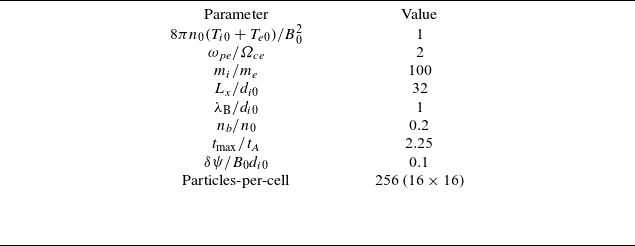
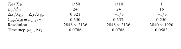


 Open access