


1. Introduction
Density-driven, predominantly horizontal flows in the form of gravity currents play a central role in a host of natural processes, as well as in numerous engineering applications (Simpson Reference Simpson1982). The interaction of such gravity currents with a dense bottom layer can give rise to rich and complex dynamics (Samothrakis & Cotel Reference Samothrakis and Cotel2006a,Reference Samothrakis and Cotelb; Monaghan Reference Monaghan2007; He et al. Reference He, Zhao, Lin, Hu, lv, Ho and Lin2017, Reference He, Zhao, Zhu and Hu2019; Ouillon et al. Reference Ouillon, Meiburg, Ouellette and Koseff2019a; Ouillon, Meiburg & Sutherland Reference Ouillon, Meiburg and Sutherland2019b; Tanimoto, Ouellette & Koseff Reference Tanimoto, Ouellette and Koseff2020). An interesting example in this regard concerns the sundowner winds near Santa Barbara, California, which propagate down the southern slope of the Santa Ynez Mountains. When they encounter the denser marine atmospheric boundary layer above the ocean, they can trigger internal gravity waves at the top of this layer (Smith, Hatchett & Kaplan Reference Smith, Hatchett and Kaplan2018; Carvalho Reference Carvalho2020). Similar processes may occur in estuaries when river outflows interact with a dense bottom layer near the seafloor, or in the context of effluents from desalination plants (Lattemann & Amy Reference Lattemann and Amy2013). For example, near the southern end of the Dead Sea such a dense bottom layer has been observed to form as a result of the very salty discharge from a desalination plant, and the question arises as to whether gravity currents might be able to remove or dilute this dense bottom layer.
The majority of the above studies have focused on situations in which a gravity current travelling down an inclined slope encounters a stably stratified interface. Depending on the slope angle, the relative densities of the gravity current and the ambient fluid layers, the interaction between the current and the interface can result in the formation of an intrusion and/or a dense underflow, and it can trigger the emergence of internal gravity waves. By contrast, the present investigation aims to shed light on how a gravity current can trigger interfacial waves and bores in the situation where the bottom boundary is horizontal, and how a dense bottom layer can be removed by means of a gravity current. Towards this end we focus on the model problem sketched in figure 1. We consider a two-dimensional (2-D) tank of length  $\hat {L}$ and height $\hat {H}$. Initially, the bottom of the entire tank is occupied by a shallow, dense fluid layer of depth $\hat {h}_L$ and density $\hat {\rho }_L$. Above this dense bottom layer, the left-hand section of length $\hat {L}_U$ and height $\hat {h}_U$ is filled entirely with fluid of intermediate density $\hat {\rho }_U$, while the right-hand section holds ambient light fluid of density $\hat {\rho }_0$. At time $\hat {t}=0$ we remove the gate that separates the light fluid from the intermediate density fluid, so that a right-propagating gravity current forms on top of the dense bottom layer. As the density interface is deformed by this advancing gravity current, it will give rise to interfacial perturbations whose propagation velocity may or may not exceed the front velocity of the gravity current, so that we expect different flow regimes to emerge as the ratio of these velocities varies. We remark that the present study focuses on full-depth lock release flows only, and that $\hat {L}_U$ was chosen sufficiently large so that its precise value does not have a strong effect on the results.
The initial set-up: above a dense layer of uniform thickness that covers the bottom of the entire tank, intermediate density fluid is placed in the left-hand compartment, while light fluid fills the right-hand compartment. At time  $t=0$ the gate separating the two compartments is removed, so that a gravity current forms that propagates to the right while interacting with the dense fluid layer.

We note that the situation sketched in figure 1 differs in several key aspects from the one in which all of the fluid initially to the left of the gate is of the same intermediate density, so that a dense bottom layer exists only to the right of the gate. This set-up has been explored in some detail, going back to the early experimental investigations by Holyer & Huppert (Reference Holyer and Huppert1980) and Britter & Simpson (Reference Britter and Simpson1981), and it can exhibit interesting symmetry properties. The so-called doubly symmetric configuration is obtained when the ambient layers have equal depths and the density of the fluid to the left of the gate is the average of the ambient densities. Even when the ambient fluid layers are unequal in depth, a certain dynamic symmetry holds as long as the density of the lock fluid corresponds to the depth-weighted mean density of the two ambient layers (Sutherland, Kyba & Flynn Reference Sutherland, Kyba and Flynn2004). When this condition is satisfied, the interface ahead of the intrusion remains flat, whereas otherwise a leading waveforms. The effect of small deviations from this symmetric configuration can be captured by a perturbation analysis (Sutherland et al. Reference Sutherland, Kyba and Flynn2004). Various aspects of this flow configuration, such as front velocity, velocity structure and wave excitation were further analysed by Cheong, Kuenen & Linden (Reference Cheong, Kuenen and Linden2006), Flynn & Linden (Reference Flynn and Linden2006), Lowe, Linden & Rottman (Reference Lowe, Linden and Rottman2002), Mehta, Sutherland & Kyba (Reference Mehta, Sutherland and Kyba2002) and Ooi, Constantinescu & Weber (Reference Ooi, Constantinescu and Weber2007), as well as by De Rooij, Linden & Dalziel (Reference De Rooij, Linden and Dalziel1999), who focused on the dynamics of a corresponding particle-laden flow. Khodkar, Nasr-Azadani & Meiburg (Reference Khodkar, Nasr-Azadani and Meiburg2016) proposed theoretical models for both the symmetric and non-symmetric variants of such flows, based on the conservation principles of mass and vorticity. This approach, which does not require closure assumptions for the pressure variable, reproduces the experimentally observed symmetry properties, and it yields good quantitative agreement regarding various properties of the evolving flow field. We remark that, by its very nature, the configuration sketched in figure 1 with a dense fluid layer also to the left of the gate cannot give rise to corresponding geometric or dynamical flow symmetries, since it does not produce a left-propagating countercurrent along the bottom wall. Hence it represents an interesting subject of exploration in its own right.
This paper is organized as follows. Section 2 describes the computational model, including the governing equations, initial and boundary conditions and the numerical approach. In § 3, we analyse the dynamic behaviour of the gravity current and the dense bottom fluid layer in detail, to demonstrate the existence of different flow regimes. Based on numerical observations, we develop a semiempirical model that is able to reproduce several of the flow features quantitatively. Subsequently, we propose a more comprehensive vorticity-based model that does not require any empirical closure assumptions. Furthermore, we analyse the conversion of potential to kinetic energy in some detail, along with the energy transfer among the different fluids. Finally, § 4 summarizes our findings and presents the main conclusions.
2. Computational model
2.1. Governing equations
We assume that all density variations are due to different concentrations of the same scalar, which we will refer to as ‘salinity’ in the following. After invoking the Boussinesq approximation, the dimensional governing equations for the conservation of mass, momentum and concentration take the form
 \begin{gather} \frac{\partial\hat{u}_j}{\partial\hat{x}_j}=0, \end{gather}
 \begin{gather}\frac{\partial\hat{u}_i}{\partial\hat{t}}+\hat{u}_j\frac{\partial\hat{u}_i}{\partial\hat{x}_j} ={-}\frac{1}{\hat{\rho}_0}\frac{\partial\hat{p}}{\partial\hat{x}_i} +\hat{\nu}\frac{\partial^2\hat{u}_i}{\partial\hat{x}_j\partial\hat{x}_j} +\frac{\hat{\rho}-\hat{\rho}_0}{\hat{\rho}_0}\hat{g}e^{g}_i, \end{gather}
 \begin{gather}\frac{\partial\hat{s}_U}{\partial\hat{t}}+\hat{u}_j\frac{\partial\hat{s}_U}{\partial\hat{x}_j} =\hat{\kappa}_s\frac{\partial^2\hat{s}_U}{\partial\hat{x}_j\partial\hat{x}_j}, \end{gather}
 \begin{gather} \frac{\partial\hat{s}_L}{\partial\hat{t}}+\hat{u}_j\frac{\partial\hat{s}_L}{\partial\hat{x}_j} =\hat{\kappa}_s\frac{\partial^2\hat{s}_L}{\partial\hat{x}_j\partial\hat{x}_j}. \end{gather}
Here  $\hat {u}$ denotes the fluid velocity, with the subscripts $i$,
$i$,  $j$ indicating the $x$- and $y$-direction, respectively. The upper boundary of the dense fluid layer is located at $y=0$. Here $\hat {t}$ represents time, $\hat {\rho }$ the local density, $\hat {\nu }$ the kinematic viscosity and $\hat {\kappa }_s$ the diffusivity of salt. The gravitational acceleration $\hat {g}$ points in the direction of the unit normal vector $e^{g}_{i}=(0,-1)$. The salinity values of the upper-layer lock fluid and the bottom layer are denoted by $\hat {s}_U$ and $\hat {s}_L$, respectively. By keeping track of these separately, we are able to obtain more detailed information on the Lagrangian motion of the different initial fluid regions, for example on the interface between the current and the dense layer, about their mixing behaviour, and regarding the exchange of energy between the gravity current and the dense layer fluids, with minimal additional computational expense.
We assume a linear density–salinity relationship with the expansion coefficient  $\beta$
 \begin{equation} \hat{\rho}=\hat{\rho}_0+\beta(\hat{s}_U+\hat{s}_L), \end{equation}
so that for the initial salinity values  $\hat {s}_{U,init}$ and $\hat {s}_{L,init}$ we obtain
 \begin{gather} \hat{\rho}_U=\hat{\rho}_0+\beta\hat{s}_{U,init}, \end{gather}
 \begin{gather}\hat{\rho}_L=\hat{\rho}_0+\beta\hat{s}_{L,init}. \end{gather}
We non-dimensionalize the governing equations by introducing characteristic scales of the form
 \begin{equation} x=\frac{2\hat{x}}{\hat{h}_U},\quad u=\frac{\hat{u}}{\hat{u}_b}, \quad t=\frac{2\hat{t}\hat{u}_b}{\hat{h}_U}, \quad p=\frac{\hat{p}}{\hat{\rho}_0\hat{u}^{2}_{b}}, \quad s_U=\frac{\hat{s}_U}{\hat{s}_{U,init}}, \quad s_L=\frac{\hat{s}_L}{\hat{s}_{L,init}}, \end{equation}
where  $\hat {u}_b = \sqrt {\hat {g}\hat {h}_U(\hat {\rho }_U-\hat {\rho }_0) / 2\hat {\rho }_0}$ indicates the buoyancy velocity. In this way, we arrive at the non-dimensional equations
 \begin{gather} \frac{\partial u_j}{\partial x_j}=0, \end{gather}
 \begin{gather}\frac{\partial u_i}{\partial t}+u_j\frac{\partial u_i}{\partial x_j} ={-}\frac{\partial p}{\partial x_i}+\frac{1}{Re} \frac{\partial^2 u_i}{\partial x_j\partial x_j}+(s_U+R_Ls_L)e^{g}_i, \end{gather}
 \begin{gather}\frac{\partial s_U}{\partial t}+u_j\frac{\partial s_U}{\partial x_j} =\frac{1}{Pe}\frac{\partial^2 s_U}{\partial x_j\partial x_j}, \end{gather}
 \begin{gather}\frac{\partial s_L}{\partial t}+u_j\frac{\partial s_L}{\partial x_j}=\frac{1}{Pe}\frac{\partial^2 s_L}{\partial x_j\partial x_j}. \end{gather}
As governing dimensionless parameters, we obtain the Reynolds number,  $Re$,
$Re$,
 \begin{equation} Re=\frac{\hat{u}_b\hat{h}_U}{2\hat{\nu}}, \end{equation}
the Péclet number,  $Pe$,
$Pe$,
 \begin{equation} Pe=\frac{\hat{u}_b\hat{h}_U}{2\hat{\kappa}_s}, \end{equation}
the density parameter,  $R_L$,
 \begin{equation} R_L=\frac{\hat{\rho}_L-\hat{\rho}_0}{\hat{\rho}_U-\hat{\rho}_0}, \end{equation}
where  $Re$ and $Pe$ are related by the Schmidt number $Sc$ as follows:
 \begin{equation} Sc = \frac{Pe}{Re} = \frac{\hat{\nu}}{\hat{\kappa}_s}. \end{equation}
In the following we set  $Sc=1$, based on observations by earlier authors who found that for similar flows the value of $Sc$ has a negligible effect, as long as it is at least unity (Necker et al. Reference Necker, Härtel, Kleiser and Meiburg2005). The evolving gravity current is thus fully characterized by $Re$,
$Re$,  $R_L$ and the dimensionless thickness $h_L$ of the bottom fluid layer. In the following, we will focus on the influence of $R_L$ and $h_L$, by discussing simulation results for sufficiently high Reynolds numbers so that the precise value of $Re$ is of minor importance.
2.2. Initial and boundary conditions
Unless otherwise noted, the tank extends over  $L=80$, with a lock length $L_U=10$. No-slip conditions are enforced along the bottom and sidewalls, while the upper boundary is modelled as a free surface by implementing a non-deformable slip wall. The salinity field is subject to no-flux conditions along all boundaries. Initially, the fluid is at rest everywhere. We will discuss results from a total of 13 simulations, whose parameters are listed in table 1.
Overview of the simulations conducted and the associated parameter values.

2.3. Numerical method
All simulations are conducted with our in-house incompressible Navier–Stokes solver PARTIES, which employs second-order central finite differences to discretize the viscous and diffusive terms, along with a second-order upwind scheme for the advection terms (Biegert, Vowinckel & Meiburg Reference Biegert, Vowinckel and Meiburg2017a; Biegert et al. Reference Biegert, Vowinckel, Ouillon and Meiburg2017b). Time integration is performed by means of a third-order low-storage Runge–Kutta method. The pressure-projection method is implemented, based on a direct fast Fourier transform solver for the resulting Poisson equation at each Runge–Kutta substep. Validation results presented by Nasr-Azadani & Meiburg (Reference Nasr-Azadani and Meiburg2011) and Nasr-Azadani, Hall & Meiburg (Reference Nasr-Azadani, Hall and Meiburg2013) indicate that the uniform mesh size  $l$ should satisfy
 \begin{equation} l<\frac{1}{\sqrt{Re Sc}}. \end{equation}
Accordingly, we employ  $l=0.01$ in all simulations. To demonstrate convergence of the numerical results, we simulated run 6 also for a finer grid with $l=0.005$. The interfacial shape is shown in figure 2 by means of the contour $s_L=0.5$ at $t=15$. Ahead of and behind the gravity current, the interfacial waveforms of the two simulations are in close agreement, which indicates that the results are converged. On the other hand, the chaotic, vortical nature of the flow near the interfacial region between the bottom layer and the gravity current prevents a similarly close agreement in this region, or a strict power-law convergence of the interfacial shapes. Nevertheless, moving average values for the interface locations in this region are very close.
The interfacial waveforms for run 6 for different grid spacings at  $t=15$, as obtained from the shape of the contour $s_L=0.5$. The close agreement between the two lines indicates that the simulations are converged.

2.4. Two-dimensional versus three-dimensional simulations
In order to assess the importance of three-dimensional (3-D) effects, we ran a 3-D simulation for the same parameters as run 6. The width of the computational domain in the spanwise  $z$-direction was $2.4$. Figure 3 compares the dimensionless density fields at various times for the 2-D case (panels (a), (c) and (e)) with the spanwise average for the 3-D simulation (panels (b), (d) and (f)). The flow at early times ( $t=5$) after the release is similar for the 2-D and 3-D simulations. During the later stages ( $t=20$ and 40), the Kelvin–Helmholtz vortices are more pronounced in the 2-D simulation than in three dimensions. However, such quantities as the front location and the terms in the energy equation, shown in figure 4, are essentially identical in two and three dimensions. Details regarding the front location and energy terms will be discussed in §§ 3.1 and 3.5, respectively. Hence we conclude that the addition of the third dimension in the simulations has only a weak effect on those key features that are the focus of the present investigation.
Dimensionless density fields for 2-D and 3-D simulations with  $R_L=2$ and $h_L=0.4$: panels (a), (c) and (e) show the 2-D results at $t=5$, 20 and 40; panels (b), (d) and (f) show the corresponding 3-D results at the same times. While the Kelvin–Helmholtz vortices are more pronounced in the 2-D simulation, the shapes of the undular bores are nearly identical in two and three dimensions.

Time history of the front location and energy budget terms for the 2-D and 3-D simulations with  $R_L=2$ and $h_L=0.4$: (a) front position of the gravity current $X_f$ and location of the wave $X_w$; (b) potential energy of the gravity current $E_{pU}$ and dense layer fluid $E_{pL}$. The 2-D and 3-D results show close agreement.

3. Results
3.1. Flow regimes
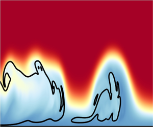
The density fields shown in figure 5 illustrate some of the flow patterns that can emerge for different values of the density parameter  $R_L$, if the lower layer thickness is held at a constant value $h_L=0.2$. For the densest bottom layer with $R_L=5$, we observe the formation of a small-amplitude undular bore at the interface between the upper and lower layers that propagates significantly faster than the gravity current front. The amplitudes of the wave crests that follow the bore front remain much smaller than the gravity current height throughout the simulation.
Dimensionless density fields for a constant lower layer thickness  $h_L=0.2$, and different values of the density ratio $R_L$: (a) run 4 with $R_L=5$; (b) run 3 with $R_L=2$; (c) run 2 with $R_L=1.43$. For smaller density contrasts the interfacial waves propagate more slowly, and they increase in amplitude. The black contour represents the value $s_U=0.1$.

For the intermediate density bottom layer with  $R_L=2$, the perturbation evolving along the interface between the lower and upper layers propagates significantly more slowly, although still faster than the gravity current front. Rather than an undular bore, we observe a train of distinct nonlinear individual waves whose amplitude is comparable to the gravity current height. The front velocity of the gravity current remains similar to that of the $R_L=5$ case, as shown in figure 6.
Position  $X_f$ of the gravity current front (dashed lines) and location $X_w$ of the leading interfacial wave (solid lines) for the flows shown in figure 5, as functions of time. The density ratio $R_L$ has a strong influence on the interfacial wave velocity, whereas its effect on the gravity current velocity is small.

Finally, for  $R_L=1.43$ the perturbation along the interface between the upper and lower fluid layers slows down even further, although the gravity current velocity remains essentially unchanged. A significant amount of gravity current fluid becomes entrained into the emerging large-amplitude interfacial wave, before this wave separates from the gravity current front and propagates a short distance ahead of it. Furthermore, we note that shear-generated Kelvin–Helmholtz waves evolve along the interfaces between the gravity current and the ambient, and the gravity current and the dense bottom layer.
Figure 6 shows the front locations of the gravity currents,  $X_f$, and of the bore or internal waves, $X_w$, as functions of time. Here, we define the gravity current front as the rightmost location in the flow field with $s_U>0.2$, which excludes the gravity current fluid entrained into the waves in runs 2 and 3 from being considered. The front of the bore or internal wave is evaluated as the foremost point above $y=0.1$ with $s_L=0.5$. The graph indicates that the bore or internal waves move with approximately constant velocity, while the gravity current velocity varies somewhat with time. Larger values of $R_L$ result in faster interfacial waves, but they do not alter the gravity current velocity appreciably.
Figure 7 shows the corresponding density fields for simulations with a constant density ratio  $R_L=1.43$ and different bottom layer thicknesses $h_L$. For the thickest lower layer with $h_L=0.6$ an undular bore forms at the interface. The relatively long waves following the bore exhibit comparatively small amplitudes. For the intermediate lower layer thickness of $h_L=0.4$, the waves propagate more slowly, their amplitude increases, and their wavelength is reduced. This trend is even more pronounced in the thinnest lower layer with $h_L=0.2$.
Dimensionless density fields for a constant density ratio  $R_L=1.43$, and different values of the layer thickness $h_L$: (a) run 8 with $h_L=0.6$; (b) run 5 with $h_L=0.4$; (c) run 2 with $h_L=0.2$. For thinner bottom layers the interfacial waves propagate more slowly, and they increase in amplitude. The black contour represents the value $s_U=0.1$.

In order to arrive at quantitative descriptions of these qualitatively different flow fields, we now proceed to analyse the dependence of the bore, internal wave and gravity current velocities on  $R_L$ and $h_L$.
3.2. Gravity current, undular bore and internal wave velocities
Several analytical models exist for predicting the front velocity of inviscid gravity currents propagating over a solid wall. In his classical analysis, Benjamin (Reference Benjamin1968) obtains the dimensionless front velocity as
 \begin{equation} U_{f,B}=\frac{\hat{U}_{f,B}}{\hat{u}_b}=\sqrt{\frac{2\alpha(1-\alpha)(2-\alpha)}{\sigma(1+\alpha)}}, \end{equation}
where  $\sigma =\hat {\rho }_0/\hat {\rho }_U$ and $\alpha =\hat {h}_{gc}/\hat {h}_U$, with $\hat {h}_{gc}$ denoting the gravity current height and $\hat {h}_U$ the initial height of the gravity current fluid in the lock. By focusing on the conservation of vorticity, Borden & Meiburg (Reference Borden and Meiburg2013a) derive a corresponding dimensionless result for Boussinesq currents in the form
 \begin{equation} U_{f,BM}=\frac{\hat{U}_{f,BM}}{\hat{u}_b}=2\sqrt{\alpha}(1-\alpha). \end{equation}
For a Boussinesq gravity current with height equal to half the upper fluid layer thickness, so that  $\sigma = 1$ and $\alpha =1/2$, both of these relationships predict a dimensionless front velocity of $1/\sqrt {2} \approx 0.71$. Figure 8(a) indicates that this value provides a reasonably good estimate of the computationally observed, fluctuating gravity current front velocities for runs 2, 3 and 4, which suggests that these gravity currents behave approximately as half-depth currents.
(a) The gravity current front velocity  $U_f$ for runs 2, 3 and 4 as a function of time. The dashed blue line represents the predicted velocity of $1/\sqrt {2}$ for half-depth currents. The average front velocity for all three gravity currents is close to this value, which suggests that the gravity currents behave approximately as half-depth currents. (b) The undular bore or leading internal wave velocity $U_w$ for runs 2, 3 and 4 as a function of time.

Figure 8(b) shows the velocity  $U_w$ of the bore or internal waves as a function of time, again for runs 2, 3 and 4. After an initial acceleration phase a quasisteady state emerges that is characterized by an approximately constant wave speed. In order to quantify this quasisteady bore or wave velocity, we refer to the circulation model of Borden & Meiburg (Reference Borden and Meiburg2013b), which predicts the propagation velocity of an inviscid bore advancing over a solid wall as
 \begin{equation} U_{w,BM}=\frac{\hat{U}_{w,BM}}{\hat{u}_b}=\sqrt{\frac{2R_Lh_L}{h_U}}\sqrt{\frac{2R^2(Rr-1)^2}{R-2Rr+1}}. \end{equation}
Here  $r=\hat {h}_L/(\hat {h}_L+\hat {h}_U)$ and $R=\hat {h}_{ep}/\hat {h}_L$, where $\hat {h}_{ep}$ denotes the lower layer thickness behind the bore. For the flows shown in figure 5, which have undular bores or internal waves, we do not have a constant lower fluid layer thickness behind the bore, so that we define an effective equilibrium layer thickness $\hat {h}_{ep}$ instead. This is accomplished by taking the average height of the wavy salinity contour $s_L=0.5$ between the first and the last peak, as indicated in figure 9 for runs 2, 3 and 4.
The waveforms of the bore and internal waves, as obtained from the shape of the contour  $s_L=0.5$: (a) run 4 with $R_L=5$ and $h_L=0.2$ at $t=59$; (b) run 3 with $R_L=2$ and $h_L=0.2$ at $t=73$; (c) run 2, with $R_L=1.43$ and $h_L=0.2$ at $t=80$. The dotted lines indicate the respective equilibrium heights $h_{ep}$, which are obtained by averaging the layer thickness between the first and last peak.

We remark that in the limit of small bore amplitudes,  $R=1$, the bore velocity obtained from (3.3) takes the form
 \begin{equation} U^{lim}_{w,BM}=\sqrt{\frac{2R_Lh_L}{h_U}}\sqrt{1-r}=\sqrt{\frac{2R_Lh_L}{H}}, \end{equation}
which recovers the dimensionless propagation velocity of linear shallow-water waves (Kundu & Cohen Reference Kundu and Cohen2001)
 \begin{equation} C_0=\frac{\hat{C}_0}{\hat{u}_b}=\sqrt{\frac{\hat{g}(\hat{\rho}_L-\hat{\rho}_0)\hat{h}_U\hat{h}_L}{\hat{\rho}_0\hat{H}\hat{u}^2_b}} =\sqrt{\frac{2h_LR_L}{H}}. \end{equation}
 Figure 10 compares the value of the front velocity  $U_w$ from the simulation with the value $U_{w,BM}$ predicted by the model of Borden & Meiburg (Reference Borden and Meiburg2013b), for all flows that exhibit a bore or a train of waves. We find that the propagation velocities observed in the simulations are close to, although generally approximately 5 %–10 % below the values predicted by the model, likely because the model neglects the effects of viscosity. It is interesting to note that the velocity of the train of large-amplitude, distinct internal waves in runs 2 and 3 is predicted quite well by treating this wave train as an equivalent bore whose height equals the average height of the wave train.
Comparison of the bore/internal wave propagation velocity  $U_w$ from the simulations with the value $U_{w,BM}$ predicted by the circulation-based model of Borden & Meiburg (Reference Borden and Meiburg2013b).

3.3. Effective bore height
The above results suggest that the gravity current behaves approximately as a half-depth current with  $h_{gc}=1$, and they indicate that the circulation-based model of Borden & Meiburg (Reference Borden and Meiburg2013b) yields a good estimate of the bore velocity as a function of the effective bore height $h_{ep}$. In order to obtain a closed, predictive model of the evolving flow field without any adjustable constants, we still require knowledge of this effective bore height as a function of $R_L$ and $h_L$. In order to obtain this relationship, we focus on the detailed formation process of the undular bore and the accompanying internal waves as shown in figure 11, for the representative flow of run 6. Upon removal of the gate, the evolving gravity current erodes some of the dense fluid at the bottom of the tank, which then accumulates ahead of the gravity current front. The front pushes this dense lower layer fluid towards the right-hand side, so that it forms a bore that propagates faster than the current front itself. As this bore separates from the gravity current front, a series of internal waves form in its wake.
Details of the undular bore formation process for run 6, with  $R_L=2$ and $h_L=0.4$. Shown is the dimensionless density field at various times, along with the $s_U=0.1$ contour. The gravity current erodes part of the bottom layer of dense fluid, which accumulates ahead of the current front and produces an undular bore that propagates more rapidly than the gravity current itself.

A prediction of the effective bore height  $h_{ep}$ as a function of $R_L$ and $h_L$ can be obtained from the simplified flow model sketched in figure 12. Towards this end, we hypothesize that the depth to which the current penetrates into the lower layer is dictated by the condition that the hydrostatic pressures $p_1=p_2$, which yields
 \begin{equation} h_1R_L+h_{gc}=h_{ep}R_L . \end{equation}
With the earlier observation that  $h_{gc} \approx 1$, we thus obtain
 \begin{equation} h_{ep}-h_1=\frac{1}{R_L} . \end{equation}
Simplified model for estimating the equilibrium depth  $h_{ep}$ of the dense fluid layer behind the bore, based on the assumptions that $h_{gc} \approx 1$ and that the hydrostatic pressures $p_1$ and $p_2$ are in balance.

The volumetric rate at which the gravity current erodes the dense fluid layer is  $U_f (h_{ep}-h_1) = U_f/R_L$, so that the mass balance for the elevated interfacial region between the gravity current front and the bore yields
 \begin{equation} \frac{U_f}{R_L} = U_w (h_{ep}-h_L). \end{equation}
Keeping in mind that  $h_{gc} \approx 1$, we have $U_f \approx 1/\sqrt {2}$. Along with (3.3), we substitute this into (3.8) to obtain
 \begin{equation} \frac{1}{4R^3_L}=\frac{h^2_{ep}(h_{ep}-h_L)^2[h_{ep}h_L-h_L(h_L+2)]^2}{h^2_L(h_L+2)[(h_{ep}+h_L)(h_L+2)-2h_{ep}h_L]}, \end{equation}
which predicts  $h_{ep}$ implicitly as a function of $R_L$ and $h_L$. Figure 13 indicates that the values of $h_{ep}$ predicted by (3.9) agree reasonably well with the values observed in the simulations, as reflected by the coefficient of determination (‘goodness of the fit’), $R^2=0.86$.
Comparison of the simulation values for the equilibrium layer height  $h_{ep}$ behind the bore, and the corresponding values predicted from (3.9).

3.3.1. Ratio of gravity current to linear wave velocity
Sutherland et al. (Reference Sutherland, Kyba and Flynn2004) draw attention to the important role played by the ratio of the gravity current front velocity to the propagation velocity of linear waves along the interface between the ambient and the lower layer fluids. Their experiments show that the small-amplitude linear waves observed forming for subcritical gravity currents transition to large-amplitude solitary waves when the gravity current propagates at supercritical speeds. We will now discuss the influence of this ratio for the present flow configuration.
Figure 14 shows the linear wave velocity  $C_0$ as a function of $\sqrt {h_LR_L/H}$, along with the velocity $U_{f,B}=1/\sqrt {2}$ of half-depth gravity currents predicted by Benjamin (Reference Benjamin1968) and Borden & Meiburg (Reference Borden and Meiburg2013a). The two velocities are equal for $\sqrt {h_LR_L/H}=1/2$. When $\sqrt {h_LR_L/H}>1/2$, small interfacial waves propagate away from the gravity current front, and a large-amplitude bore does not form. This holds for runs 4 and 6–10. For $\sqrt {h_LR_L/H} < 1/2$, on the other hand, small waves cannot outrun the gravity current. Hence a larger undular bore or a train of high-amplitude waves emerges whose propagation velocity $U_w$ exceeds that of linear waves, as can be seen for runs 2, 3, 5, 12 and 13.
Gravity current velocity  $U_f$ and bore velocity $U_w$ observed in the simulations, as functions of $\sqrt {h_LR_L/H}$. Also shown are the linear shallow-water wave velocity $C_0$ and the predicted half-depth gravity current front velocity $U_{f,B}=1/\sqrt {2}$. For $C_0 > 1/\sqrt {2}$ a small-amplitude bore forms that outruns the gravity current, whereas for $C_0 < 1/\sqrt {2}$ we observe large-amplitude waves that propagate at roughly the same velocity as the gravity current front.

3.3.2. Amplitude and wavelength of the undular bore waves
We take half of the average vertical distance between adjacent crests and troughs as the amplitude  $a$, and twice the average horizontal distance as the wavelength $\lambda$. Figure 15(a) shows that the amplitude $a$ decreases with larger $h_L$ and $R_L$. Figure 15(b) indicates that the wavelength $\lambda$ increases with larger $h_L$ and decreases with higher $R_L$.
The dependence of (a) the amplitude  $a$, and (b) the wavelength $\lambda$ of the undular bore waves, on $h_L$ and $R_L$.

3.4. Vorticity-based model
Above, we calculated  $h_{ep}$, $U_w$ and $U_f$ based on the computational observation that the gravity current behaves approximately as a half-depth current with $h_{gc} \approx 1$, and by using the empirical assumption of hydrostatic pressure balance $p_1=p_2$. In the following, we will employ the conservation of mass and vorticity to develop a more comprehensive, self-contained and closed model that does not require such empirical assumptions. The derivation of this model builds on the earlier work by Khodkar et al. (Reference Khodkar, Nasr-Azadani and Meiburg2016).
Figure 16 illustrates the flow field under consideration. After removal of the gate, the lock fluid forms a right-propagating gravity current of undetermined height  $\hat {h}_{gc}$ that propagates with velocity $\hat {U}_f$. Simultaneously, a left-propagating buoyant gravity current with density $\hat {\rho }_0$ and height $\hat {h}_u$ emerges along the top wall. Ahead of the gravity current, a bore of thickness $\hat {h}_{ep}$ propagates along the interface with velocity $\hat {U}_w$. Behind the bore front, the upper and lower layers have velocities $\hat {U}_{ub}$ and $\hat {U}_{lb}$, respectively. The flow is fully described by nine unknowns: $\hat {U}_f$, $\hat {U}_u$, $\hat {U}_w$, $\hat {U}_{ub}$, $\hat {U}_{lb}$, $\hat {h}_l$, $\hat {h}_u$, $\hat {h}_{gc}$ and $\hat {h}_{ep}$, as shown in figure 16.
Schematic of a gravity current interacting with the bottom fluid layer, for developing the vorticity-based model described in the text.

Within control volume  $DEFG$, and in the reference frame moving with the bore, mass conservation for the upper and lower layers, along with vorticity conservation along the interface give
 \begin{gather} \hat{U}_w\hat{h}_L=(\hat{U}_w-\hat{U}_{lb})\hat{h}_{ep}, \end{gather}
 \begin{gather}\hat{U}_w\hat{h}_U=(\hat{U}_w+\hat{U}_{ub})(\hat{H}-\hat{h}_{ep}), \end{gather}
 \begin{gather}\hat{g}'_L(\hat{h}_{ep}-\hat{h}_L)=\left(\hat{U}_w+\frac{\hat{U}_{ub}-\hat{U}_{lb}}{2}\right)(\hat{U}_{lb}+\hat{U}_{ub}), \end{gather}
where  $\hat {g}'_L=\hat {g}(\hat {\rho }_L-\hat {\rho }_0)/\hat {\rho }_0$.
In control volume  $CDGH$, in the reference frame moving with the intrusion, the two continuity equations for the upper and lower layers can be written as
 \begin{gather} (\hat{U}_f-\hat{U}_{lb})\hat{h}_{ep}=\hat{U}_f\hat{h}_l, \end{gather}
 \begin{gather}(\hat{U}_f+\hat{U}_{ub})(\hat{H}-\hat{h}_{ep})=(\hat{U}_f+\hat{U}_u)\hat{h}_u. \end{gather}
The vorticity conservation equations along the respective interfacial segments are
 \begin{gather} -(\hat{g}'_L-\hat{g}'_U)(\hat{h}_{ep}-\hat{h}_l)+ \frac{\hat{g}'_L-\hat{g}'_U}{\hat{g}'_L}\left(\hat{U}_f+\frac{\hat{U}_{ub}-\hat{U}_{lb}}{2}\right) (\hat{U}_{ub}+\hat{U}_{lb})={-}\frac{1}{2}\hat{U}^2_f, \end{gather}
 \begin{gather}\hat{g}'_U(\hat{H}-\hat{h}_{ep}-\hat{h}_u)+ \frac{\hat{g}'_U}{\hat{g}'_L}\left(\hat{U}_f+\frac{\hat{U}_{ub}-\hat{U}_{lb}}{2}\right) (\hat{U}_{ub}+\hat{U}_{lb})=\frac{1}{2}(\hat{U}_u+\hat{U}_f)^2, \end{gather}
where  $\hat {g}'_U = \hat {g}(\hat {\rho }_U - \hat {\rho }_0)/\hat {\rho }_0$. In addition, we have the geometrical constraint
 \begin{equation} \hat{h}_{gc} + \hat{h}_{u} + \hat{h}_{l} = \hat{H}. \end{equation}
 For control volume  $BCHI$, in the frame moving with the upper gravity current front, the vorticity conservation yields
 \begin{equation} \hat{g}'_U\hat{h}_u=\tfrac{1}{2}(\hat{U}_u+\hat{U}_f)^2. \end{equation}
After non-dimensionalization, we obtain the following system of eight coupled, nonlinear equations:
 \begin{gather} U_wh_L=(U_w-U_{lb})h_{ep}, \end{gather}
 \begin{gather}U_wh_U=(U_w+U_{ub})(H-h_{ep}), \end{gather}
 \begin{gather}R_L(h_{ep}-h_L)=\left(U_w+\frac{U_{ub}-U_{lb}}{2}\right)(U_{lb}+U_{ub}), \end{gather}
 \begin{gather}(U_f-U_{lb})h_{ep}=U_fh_l, \end{gather}
 \begin{gather}(U_f+U_{ub})(H-h_{ep})=(U_f+U_u)h_u, \end{gather}
 \begin{gather}(1-R_L)(h_{ep}-h_l)+\frac{R_L-1}{R_L}\left(U_f+\frac{U_{ub}-U_{lb}}{2}\right)(U_{ub}+U_{lb})={-}\frac{1}{2}U^2_f, \end{gather}
 \begin{gather}H-h_{ep}-h_u+\frac{1}{R_L}\left(U_f+\frac{U_{ub}-U_{lb}}{2}\right)(U_{ub}+U_{lb})=\frac{1}{2}(U_u+U_f)^2, \end{gather}
 \begin{gather}h_u=\tfrac{1}{2}(U_u+U_f)^2. \end{gather}
Note that we have already eliminated  $\hat {h}_{gc}$ by making use of the geometrical constraint. This system can be solved efficiently with the MATLAB function vpasolve.
Figure 17(a) shows values of the gravity current height  $h_{gc}$ predicted by the model, as a function of $R_L$ and $h_L$, along with the corresponding simulation results. Here the gravity current height for the simulation is obtained by time-averaging over $10 < t < 25$ the quantity
 \begin{equation} h_{gc}=\int^{h_U}_{h_U-H}s_U \, \textrm{d} y \end{equation}
at the gate location  $x=10$. The simulation results are generally within approximately $10\,\%$ of the vorticity model predictions. Especially for smaller values of $R_L$, the predicted and simulated intrusion heights are substantially larger than the value $h_{gc}=1$ that we had assumed for the earlier empirical model that resulted in (3.9), which highlights the limitations of that model. For $h_L>0.2$, the predicted intrusion thickness $h_{gc}$ varies only weakly with $h_L$.
The dependence of (a)  $h_{gc}$, (b) $h_{ep}$ and (c) $U_w$ on $R_L$ and $h_L$. The black and blue numbers indicate simulation results and values predicted by the model, respectively.

Figure 17(b) shows predictions by the vorticity model for the equilibrium height  $h_{ep}$, which is seen to vary approximately linearly with the height of the bottom fluid layer $h_L$. For $R_L<3$, $h_{ep}$ decreases rapidly as $R_L$ grows, which reflects the fact that denser bottom layers are less easily removed by gravity currents. The predictions by the vorticity models generally lie within approximately $10\,\%$ of the simulation data.
Vorticity model predictions for the bore velocity  $U_w$ are presented in figure 17(c). Just as we had seen for the other flow variables, the predictions are reasonably close to the corresponding simulation data, and they show that $U_w$ increases with $h_L$ and $R_L$, consistent with the shallow water wave speed given by (3.5).
3.5. Energy budget
In applications where a dense bottom layer is to be removed by means of employing a gravity current, the only source of energy that we have available for dislodging the dense fluid is the potential energy initially contained in the gravity current fluid. This energy then needs to be transferred to the dense bottom layer in order to dislodge it. Hence, it is of interest to study how efficiently the potential energy of the gravity current fluid is converted into potential and kinetic energy of the dense bottom fluid. Towards this end, we define the potential energy  $E_p$, kinetic energy $E_k$ and dissipated energy $E_d$ of the flow, respectively, as
 \begin{gather} E_p(t)=\int^{h_U}_{h_U-H}\int^L_0 (s_U+R_Ls_L)y \, \mathrm{d} x\, \mathrm{d} y, \end{gather}
 \begin{gather}E_k(t)=\int^{h_U}_{h_U-H}\int^L_0\tfrac{1}{2}(u^2+v^2) \, \mathrm{d} x\, \mathrm{d} y, \end{gather}
 \begin{gather}E_d(t)=\int^t_0\varepsilon(\tau) \, \mathrm{d}\tau . \end{gather}
Note that the potential energy is evaluated relative to a situation with ambient fluid everywhere, and relative to the initial lower boundary of the gravity current and ambient fluids at  $y=0$. Here $\varepsilon$ indicates the instantaneous viscous dissipation rate
 \begin{equation} \varepsilon(t) = \int^{h_U}_{h_U-H}\int^L_0 \frac{2}{Re}s_{ij}s_{ij} \, \mathrm{d} x\, \mathrm{d} y, \end{equation}
with  $s_{ij}$ denoting the rate-of-strain tensor
 \begin{equation} s_{ij} = \frac{1}{2}\left(\frac{\partial u_i}{\partial x_j}+\frac{\partial u_j}{\partial x_i}\right). \end{equation}
Since the fluid is at rest initially, the overall energy budget of the flow thus takes the form
 \begin{equation} E_{total}=E_p+E_k+E_d=\mathrm{const.}=E_{p,init} \end{equation}
where  $E_{p,init}$ represents the initial potential energy. In order to investigate the time-dependent exchange of potential and kinetic energy, and the energy transfer from the gravity current to the dense lower layer and to the ambient fluid, we consider their respective contributions to the overall energy budget
 \begin{gather} E_k=E_{kU}+E_{kL}+E_{k0}, \end{gather}
 \begin{gather}E_p=E_{pU}+E_{pL}, \end{gather}
 \begin{gather}E_d=E_{dU}+E_{dL}+E_{d0}, \end{gather}
 \begin{gather}\varepsilon=\varepsilon_U+\varepsilon_L+\varepsilon_0, \end{gather}
where the subscripts  $_U$,
$_U$,  $_L$ and $_0$ again refer to gravity current, dense fluid layer and ambient fluid, respectively. These contributions take the form
 \begin{gather} E_{kU}(t)=\int^{h_U}_{h_U-H}\int^L_0s_U\tfrac{1}{2}(u^2+v^2) \, \mathrm{d} x\,\mathrm{d} y, \end{gather}
 \begin{gather}E_{kL}(t)=\int^{h_U}_{h_U-H}\int^L_0s_L\tfrac{1}{2}(u^2+v^2) \, \mathrm{d} x\,\mathrm{d} y, \end{gather}
 \begin{gather}E_{k0}(t)=\int^{h_U}_{h_U-H}\int^L_0(1-s_U-s_L)\tfrac{1}{2}(u^2+v^2) \, \mathrm{d} x\,\mathrm{d} y, \end{gather}
 \begin{gather}E_{pU}(t)=\int^{h_U}_{h_U-H}\int^L_0s_Uy \, \mathrm{d} x\,\mathrm{d} y, \end{gather}
 \begin{gather}E_{pL}(t)=\int^{h_U}_{h_U-H}\int^L_0R_Ls_Ly \, \mathrm{d} x\,\mathrm{d} y, \end{gather}
 \begin{gather}\varepsilon_U(t)=\int^{h_U}_{h_U-H}\int^L_0s_U\frac{2}{Re}s_{ij}s_{ij} \, \mathrm{d} x\,\mathrm{d} y, \end{gather}
 \begin{gather}\varepsilon_L(t)=\int^{h_U}_{h_U-H}\int^L_0s_L\frac{2}{Re}s_{ij}s_{ij} \, \mathrm{d} x\,\mathrm{d} y, \end{gather}
 \begin{gather}\varepsilon_0(t)=\int^{h_U}_{h_U-H}\int^L_0(1-s_U-s_L)\frac{2}{Re}s_{ij}s_{ij} \, \mathrm{d} x\,\mathrm{d} y . \end{gather}
 As a representative example, figure 18 shows the time history of all energy components for run 2, cf. figure 5. Each component is normalized by the initial potential energy of the gravity current fluid  $E_{pU,init}$. The total energy $E_{total}$ is seen to vary by less than $2\,\%$ over the course of the simulation, which reflects the good energy conservation properties of the simulation code. Over the first 15 time units, $E_{pU}$ rapidly decreases by approximately $50\,\%$, as the intermediate density lock fluid collapses and forms the gravity current. This potential energy is converted in approximately equal parts to kinetic energy of the gravity current and ambient fluids. Since we evaluate the potential energy relative to $y=0$, its initial value for the dense fluid layer is negative. However, as the dense fluid is eroded by the gravity current and forms the high-amplitude interfacial wave seen in figure 5, its potential and kinetic energies gradually increase. All three dissipated energy components $E_{dU}$, $E_{d0}$ and $E_{dL}$ remain relatively small throughout the simulation.
Time history of the various energy budget components for run 2, with  $R_L=1.43$ and $h_L=0.2$. The potential energy given up by the gravity current fluid is converted in nearly equal parts to kinetic energy of the gravity current and ambient fluids, with smaller contributions going towards raising the potential energy of the dense fluid layer, and to dissipation.

Figure 19 shows the influence of the density ratio  $R_L$ on the evolution of the individual energy budget components of the dense fluid layer. When $R_L=1$, the bottom layer has the same density as the gravity current, so that it can easily be eroded and uplifted, thereby gaining potential energy. Initially, as $R_L$ increases the potential energy gain of the lower layer decreases, as it becomes harder to lift up the dense layer fluid. Beyond $R_L=1.43$, however, the uplifted fluid contains more potential energy for larger $R_L$ even though the wave amplitude continues to decrease, due to its higher density. The high-amplitude internal waves for small $R_L$ contain more kinetic energy than the low-amplitude waves for large $R_L$, so that $E_{kL}$ decreases with increasing $R_L$. The amount of energy dissipated by the lower layer does not show a strong dependence on $R_L$.
Time history of the dense layer energy budget components for runs 1, 2, 3 and 4 with  $R_L=1$, 1.43, 2 and 5 and $h_L=0.2$. While the potential energy of the dense layer grows more rapidly for larger $R_L$ (blue lines) (except $R_L=1$), its kinetic energy grows more slowly (black lines).

Figure 20 analyses the influence of the dense fluid layer thickness  $h_L$ on the energy conversion and transfer processes. Figure 20(a) shows the evolution of the energy components in the gravity current fluid. For larger $h_L$-values, the gravity current fluid sinks more deeply into the dense fluid layer, cf. figure 7, so that it loses its potential energy $E_{pU}$ more rapidly, while its kinetic energy $E_{kU}$ increases more slowly. Consistent with this slower kinetic energy increase for larger $h_L$, the dissipated energy $E_{dU}$ is smallest for the deepest dense fluid layer.
Time history of the various energy budget components in runs 2, 5 and 8 with  $h_L=0.2$, 0.4 and 0.6, and $R_L=1.43$, together with run 11 for $h_L=0$. (a) Gravity current fluid: since the gravity current fluid sinks more deeply into thicker bottom layers, it loses its potential energy more rapidly (blue lines), while its kinetic energy increases more slowly (black lines), so that its overall energy decreases for larger $h_L$ (magenta lines). (b) Dense layer fluid: as the gravity current fluid penetrates thicker bottom layers more deeply, the dense fluid is being lifted up more strongly, so that its potential energy increases more rapidly (blue lines), as does its kinetic energy (black lines).

The time history of the various energy components for the dense fluid layer as a function of  $h_L$ is shown in figure 20(b). As we saw above, the gravity current sinks more deeply into the dense layer when this is thicker. As a result, more of the dense fluid is being lifted up, so that the potential energy gain of the bottom fluid layer increases for larger $h_L$-values. While the internal waves have a smaller amplitude for larger $h_L$, their velocity is higher, so that the dense fluid layer acquires more kinetic energy. In summary, thicker dense fluid layers see a more rapid increase in their overall energy.
4. Conclusions
We have explored the removal of a dense fluid layer above a horizontal bottom wall by a lock-release gravity current, via 2-D Navier–Stokes simulations in the Boussinesq limit. As the two dominant dimensionless quantities governing this problem, we identify a thickness parameter for the dense bottom layer, and the density ratio given by the differences between the densities of the bottom layer, the gravity current and the ambient fluid. After releasing the lock fluid, we observe the formation of a quasisteady gravity current which displaces some of the dense bottom layer fluid, so that it accumulates ahead of the gravity current and forms an undular bore or a series of internal gravity waves. These propagate ahead of the current, along the interface between the dense fluid layer and the ambient fluid. Depending on the ratio of the gravity current front velocity and the linear shallow-water wave velocity of interfacial waves, we observe the existence of different flow regimes. If the linear wave velocity is larger than the gravity current velocity, the waves quickly move ahead of, and away from, the gravity current front, and their amplitude remains small. On the other hand, when the linear wave velocity is comparable to or smaller than the gravity current velocity, the waves steepen and a train of nonlinear internal waves form whose amplitude can be comparable to the thickness of the gravity current.
The simulations indicate that the gravity current behaves similarly to a half-depth current whose front velocity can be estimated from the models of Benjamin (Reference Benjamin1968) and Borden & Meiburg (Reference Borden and Meiburg2013a). In addition, the propagation velocity of the undular bore or the train of nonlinear waves can be obtained from the vorticity model of Borden & Meiburg (Reference Borden and Meiburg2013b), after defining an equilibrium layer thickness by averaging the interface height over the individual waves. With these approximations, and with the empirical assumption that the hydrostatic pressures at the bottom wall below the gravity current front and ahead of it are in balance, we can set up a semiempirical model for predicting the rate at which dense fluid is being eroded by the gravity current.
Furthermore, we develop a more sophisticated model that does not require the above empirical assumptions, based on the conservation principles for mass and vorticity. This model is able to predict such quantities as the gravity current height, the equilibrium layer thickness and the internal wave velocity as a function of the dimensionless parameters, generally to within approximately a  $10\,\%$ accuracy.
Finally, an energy budget analysis provides information on the rates at which potential energy is converted into kinetic energy and dissipated, and on the processes by which it is transferred from the gravity current fluid to the dense layer and the ambient fluids. Both the numerical simulations and the vorticity model indicate that the gravity current sinks more deeply into thicker bottom layers, which accelerates the transfer of energy from the gravity current to the dense fluid layer. In addition, for situations with equal bottom layer thicknesses, the energy of the denser bottom layer grows more rapidly.
Funding
Funding for this work was provided under NSF grant CBET-1936358. Computational resources for this work used the Extreme Science and Engineering Discovery Environment (XSEDE), which was supported by the National Science Foundation, USA, grant no. TG-CTS150053. R.Z. thanks The National Natural Science Foundation of China (11672267) and the China Scholarship Council for providing him with a scholarship to study at UCSB.
Declaration of interests
The authors report no conflict of interest.


 Open access