

1. Introduction
The last decade has seen the development of an increasing number of numerical models designed to simulate the geometry and physical characteristics of glaciers and ice sheets under a variety of environmental conditions and time-scales. Examples range from two-dimensional glacier models for interpreting field measurements, usually on fine grids (Waddington and Clarke, 1988; Jóhannesson and others, 1989; Abe-Ouchi, 1993), to vertically integrated plan-form models, developed for coupling with climate models to study continental glaciation during the ice ages (Fastook and Chapman, 1989; Verbitsky and Oglesby, 1992; MacAyeal, 1994; Marsiat, 1994). At the upper end are a number of rather complete three-dimensional models which include coupling between the flow and temperature fields and have been applied to investigate the present-day ice sheets of Antarctica and Greenland (Budd and Jenssen, 1989; Huybrechts, 1990; Calov, 1994; Fabre and others, 1995; Greve and Hutter, 1995). Typically, these models are time-dependent and are used to simulate the response of ice sheets and glaciers to climatic changes on time-scales comparable to their reaction time-scales.
All of these ice-sheet models are based on the same basic principles of conservation of mass, momentum and heat but often differ by the employed constitutive relation, the simplifications in the force balance, the treatment of the ice–bedrock and marine boundaries, and by the details of the numerical schemes employed. One of the activities organized within the European Science Foundation network of EISMINT (European Ice Sheet Modelling Initiative) was the intercomparison of current ice-sheet models to assess how well these models simulate basic geophysical variables such as ice thickness, velocity and temperature, and to identify the most accurate and efficient numerical techniques, which could then be copied, enhanced or developed to upgrade individual models.
One can distinguish three levels of ice-sheet model comparison. At the first level, boundary conditions should be fully described and as many modelled processes and parameters as possible should be fixed. In this way, the effect of numerical approximations on how individual models solve the ice continuity, flow and temperature equations can be assessed. This level is thus meant to check how accurate and efficient various numerical schemes are. Additionally, this level can be considered as a debugging tool for the model code itself. The design of such experiments should be simple enough to allow the results to be compared and checked against analytical solutions where available.
In the second level of model testing and intercomparison, boundary conditions and model set-up should still be fixed, but individual models should be run as they are formulated by including whatever processes that are considered important together with preferred values for model parameters. At this level, the result will be influenced by the level of sophistication of the individual model. The third level should be the comparison of models applied to a real ice sheet. This should be done with standard data sets for the bedrock and the climatic forcing. Examples could be the intercomparison of existing models for the whole of Antarctica or Greenland, or the application of these models to a smaller problem elsewhere.
Values of model constants specified in the intercomparison experiments

In this paper, we discuss the outcome of the EISMINT intercomparison venture at level one. Details are presented for testing models under fixed and moving-margin conditions, for both two-dimensional vertical-plane models and two- or three-dimensional horizontal plan-form models. The experiments consider vertically integrated isothermal ice flow and may include a temperature calculation, although not thermomechanical coupling. They test both steady-state and time-dependent behaviour. Most of the present-day codes for large-scale ice-sheet models were submitted to these experiments and their output compared. The aim here is not so much to discuss the individual results which were obtained during the intercomparison process but to present a compilation of the consensus results which emerged. In this way, a basic testing package is provided for ice-sheet models, which can serve as a benchmark against which future ice-sheet model codes can be compared.
2. The ice-sheet model
The type of ice-sheet model under consideration is a so-called time-dependent continuity model for grounded ice, which for simplicity deals with isothermal ice deformation only.
2.1. Ice flow
The basic equation solved in such a model is a continuity equation for ice thickness and is
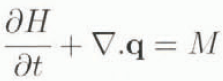
where H is ice thickness (m), q is the discharge (m2 a−1), M is the rate of surface accumulation or ablation (m a−1) and the divergence operator (∇.) can be either one- or two-dimensional.
In order to facilitate the comparison of results in these experiments, the constitutive relation is prescribed to be Glen’s flow law for the creep of polycrystalline ice (Glen, 1955; Paterson, 1994), hence
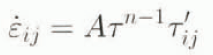
where [inline-equation] ij and τ′ ij are the components of the strain-rate and stress-deviator tensor, respectively, and [inline-equation] is the effective stress, defined as the square root of the second invariant of the stress-deviator tensor. n is the flow-law exponent and A is the rate factor, which was chosen for a temperature close to the melting point. All parameter values are defined in Table 1.
In these experiments, investigators are initially free to compute the stress and deformation fields in whatever way they deem most appropriate. However, all of the results discussed below were obtained under the standard simplifications appropriate to the shallow-ice approximation (Hutter, 1983; Morland, 1984). This means that the ice deforms only by shearing in horizontal planes and that longitudinal stress deviators are neglected in the force balance. In the case of a constant-flow parameter A, this yields the following well-known approximation for the discharge q:

where ρ is the ice density and g is the gravity.
2.2. Thermodynamics
For those models carrying out thermal calculations, the temperature distribution within the ice is calculated from the general thermodynamic equation governing the transfer of heat in a continuum:

where T is temperature (K or °C), t is the time (a), V is the three-dimensional velocity field (m a−1), F is internal heating resulting from dissipation expressed as a temperature change (Ka−1), and k and c p are thermal parameters. The degree of approximation in Equation (4) was left to the individual modeler, as were the details of the vertical discretization.
Two boundary conditions are required for Equation (4). At the upper ice-sheet surface, the mean annual air temperature (or T 0 = 273.15 K, when the air temperature is above the melting point) is used as a Dirichlet boundary condition. While at the ice–bedrock interlace, mixed boundary conditions are employed: if the ice is melting, then the pressure-melting point temperature is used as a Dirichlet boundary condition; however, if the basal ice is frozen, then the geothermal heat flux (G) is used as a Neumann boundary condition where
otherwise
and z is vertical coordinate. The pressure-melting
Numerical grid on which the benchmark calculations take place. The orientation of the axes and the numbering conventions are shown together with the steady-state ice-thickness distributions for the fixed-margin and moving-margin experiments. The cross-section for flowline models is between points (1,16) and (31,16).

point temperature T′ is given by the following relation:
where values for T 0 (triple-point temperature of ice) and β (Clausius–Clapeyron gradient) are also given in Table 1. It is understood that the ice temperature can never rise above the pressure-melting point as given by Equation (7).
It is furthermore required that all calculated ice temperatures are output as homologous temperatures, that is relative to the local pressure-melting point, in which case they are expressed in °C.
3. The experimental model set-up
Two series of experiments with idealized geometry are proposed. The numerical domain is the same in both experiments. It consists of a square grid of sides 1500 × 1500 km with a flat bed at zero elevation. The grid spacing is defined to be 50 km, leading to 31 × 31 = 961 regularly spaced points. This set-up applies to plan-form models. Flowline models calculate the cross-section from one side to the other. For ease of comparison, the righthanded coordinate system has its origin in the lower left corner. The numbering scheme has indices between (1,1) and (31,31) or between (1) and (31), where the point (1,1) coincides with the origin in plan-form models and (1) is at the lefthand side of the cross-section in flowline models. These conventions are shown in Figure 1.
As the emphasis is on testing ice physics and comparing numerical techniques, the models tested in this paper did not include basal sliding, and do not include such processes as firn densification, bedrock adjustment, thermomechanical coupling or thermal interaction with the underlying rock.
3.1. The fixed margin experiment
In this first experiment, the main feature is the artificial constraint of horizontal ice-sheet extent. The ice sheet fills the entire model grid, leading to a square shape. At the boundary points i = 1, i = 31 or j = 1, j = 31 Dirichlet conditions of H(x, y, t) = 0 are specified. These are also called VN boundary conditions after Vialov (1958) and Nye (1959). They imply a singularity at the margin because the margin has a non-zero ice discharge but (by definition) zero ice thickness. Although this does not pose a real problem in the numerical models examined here, it requires some precautions in the code to avoid the implied infinite ice velocity. In this paper, several diagnostic variables are also assigned a value of zero at the grid boundaries.
A similar constraint applies to flowline models, which consider a flow band of constant width and thus exclude horizontal flow convergence and divergence. This means that the results of flowline and plan-form models are not comparable but allows the flowline results to be compared against the analytical solution.
Climatic boundary conditions are a fixed accumulation rate over the entire grid and a surface temperature parameterized as a function of the distance to the divide. The latter parameterization ensures that the surface temperature will be independent of variations in surface elevation between models. The boundary conditions were chosen such that mixed wet and frozen conditions occur at the base, with the outer part at the pressure-melting point. These boundary conditions resemble Greenland conditions rather than Antarctic conditions so that

and

where M is expressed in m a−1 of ice equivalent. T surface in K, and d in km. In accordance with the square geometry, the distance to the summit is measured perpendicular to the coordinate axes, where x summit and y summit are both 730 km. The geothermal heat flux is constant and is taken as the standard value of 0.042 W m−2 (see Table 1).
3.2. The moving margin experiment
The second experiment includes ice ablation and aims at simulating the position of the free margin. The model setup resembles the one for the fixed-margin experiments, except for different climatic boundary conditions, i.e.
where

and

The mass-balance M is a function of the radial distance d (km) from the centre of the grid. R el is the distance at which the mass balance changes from positive to negative values and s is the slope of the mass-balance function. Their values were chosen to be respectively 450 km and 10−2 m a−1 km−1. The result is a steady-state ice-sheet configuration which is axisymmetric. This enables a comparison with flowline models, which should also consider axial symmetry. This can be conveniently implemented by including a divergence term in the continuity equation, with a flow-band width which increases linearly from 0 at the centre outwards to the margin. In the special case of a constant accumulation, the discharge is half of the one without flowline divergence.
3.3. Model runs
Experiments are performed to test both the steady-state and the time-dependent model behaviour. All simulations are over 200 000 years. The evolution to steady state from zero ice thickness occurs over a period of about 25 000 years for the ice-thickness distribution and up to 150 000 years for the temperature calculations. The latter relaxation time would become even longer when flow-temperature coupling is included. To test the time-dependent aspects of the model’s behaviour, sinusoidally varying climatic boundary conditions are imposed where


and

The periods used in these experiments are of Milankovitch time-scales and are, respectively, 20 000 and 40 000 years. The steady-state solution is specified as the initial condition. The model parameters are given in Table 1. They correspond to the standard values used in most models.
4. The eismint intercomparison results
We present a compilation of the intercomparison results, which was obtained after several rounds of data submission and subsequent correction and is therefore believed to be devoid of inadvertent programming errors. In the discussion, we shall not make a distinction between individual models but rather discuss categories of models. The main reason for this is that several of the models are very similar in design and, consequently, their results are grouped closely together. This makes individual results hard to differentiate graphically. In addition, a consensus emerged during the intercomparison as to which result should be considered as the ‘best’ solution under the given experimental set-up. This has stimulated many individual code changes and makes the identification of a specific result with a specific individual modeller no longer meaningful. Instead, we will concentrate on this consensus numerical result, which will be shown together with curves demonstrating the range within which the other solutions fell.
The definition of such a consensus result calls for some comment. In the present context, it is generally defined as the mean of all of the results from the same model group, which is self-consistent in all variables and comes closest to any known analytical solution. When an analytical solution is not available, we have simply reverted to taking an average but in this case also show the individual results. In all these calculations, clearly incorrect/unstable calculations and obvious outliers were removed.
In total, 15 ice-sheet models participated in the intercomparison tests. These models can be subdivided along several lines. The largest group of 11 models calculates ice flow on a horizontal plane and is henceforth called “3d” for simplicity. Of these 3d models, seven resolve the velocity field in the vertical and include a temperature calculation. The four remaining ones do not make calculations in the vertical. The other four models are flowline models (“2d”), of which two deal solely with ice flow and two include a thermal calculation. All models are of the finite-difference type, except for one isothermal 3d model which is based on the finite-element method, but which had exactly the same characteristics as a class of the finite-difference models defined further below.
The most striking difference between these models concerns the way the ice-mass fluxes are calculated. There are several ways to discretize the evolution equation for ice thickness, which can be written as a non-linear diffusion problem with a “diffusivity” equal to the scalar part of Equation (3) where

and

All of the finite-difference models discussed here adopt a staggered grid and consequently evaluate the mass flux q in between grid points. This is necessary because non-staggered grids are unstable as they fail to represent adequately the diffusion effects of ice flow at high wave numbers. In one-dimension, we have

where D i+½ can be constructed either directly at the midpoint using the properly centred mean ice thickness H i+½ and local surface gradient, or as the mean of two diffusivities defined on the neighbouring grid points i
Intercomparison results for the fixed-margin experiments in steady state: ice thickness, mass fluxes and velocities. Details of the different curves (2d, 3d, type I, type II) are given in the text. H(0) is the ice thickness at the divide. Displayed are mean values for each group.

and i + 1;

The first method is mass-conserving. The main disadvantage of type I schemes, however, is their generally poor stability properties, necessitating very small time steps when the time-stepping is explicit. This constraint can be overcome by making the time-stepping implicit, either on the linear pan only (evaluating diffusivities at the old time step) or by iterating on the non-linear diffusivities (e.g. Hindmarsh and Hutter, 1988; Hindmarsh and Payne, 1996). The extra work implied makes such a scheme more difficult to handle and there is no particular guarantee that the end effect will be more efficient.
The second method of constructing the mass fluxes (Oerlemans and Van der Veen, 1984) is stable for much larger time steps, explicit as well as implicit, but is not inherently mass-conserving. This will affect the accuracy of the scheme where horizontal gradients are large, for instance near the margin. We found that individual differences in the time-stepping scheme (i.e. the degree of implicitness and/or the order of accuracy) did not lead to differences significant enough to warrant a further subdivision. Participants were asked to use a time step
Summary of the intercomparison results for the fixed-margin experiment in steady state. Shown are mean values together with their standard deviation. Temperatures are relative to the pressure-melting point. # is the number of model results in each group

corresponding to an optimal trade-off between accuracy and speed.
The square domain and the uniform forcing of the fixed-margin experiment imply a four-fold symmetry, so that only half a cross-section needs to be shown for distance-dependent variables such as ice thickness, mass fluxes, velocities and basal temperatures (Fig. 1). This is also the case for the moving-margin experiment, which has axial symmetry unless the margin intersects the domain boundary and produces four-fold symmetry. Other results are shown as time series with values given every thousand years. These include the ice thickness and basal temperature at the central or summit point and several variables at a distance halfway between the domain’s centre and one of its edges. Under the grid conventions shown in Figure 1, this is the point (24,16) for plan-form models and point (24) for flowline models.
Plots of the more important variables in the intercomparison experiments are shown in Figures 2–7. In these graphs, the consensus solution is usually shown as a thick black line. The results are additionally summarized in the Tables 2–7, giving for each of the model categories mean values together with their standard deviation. Many of the results do not require extensive, comment and are purely included to document the benchmark.
Intercomparison results for the fixed-margin experiments in steady state: vertical profiles and temperatures. Details of the different curves (2d, 3d, type I, type II, Raymond, Robin) are given in the text. T(0) is the homologous basal temperature at the divide in °C below the pressure-melting point.

Intercomparison results for the fixed-margin experiments forced by sinusoidal changes in boundary conditions of periods 20 and 40 ka. R is the range of the response defined as the peak-to-peak amplitude of the last oscillation. Displayed are mean values per group.

4.1. Fixed-margin experiments
The major features of variables along the horizontal transect are presented in Figure 2 and Table 2. The most important distinction within the results can be made according to the spatial discretization scheme (type I or II). Between these two types, the thickness at the divide differs by about 2.5% and this difference becomes larger towards the margin. At the margin, the type II scheme produces a mass-conservation error of as much as 50% compared to type I. These differences are brought about by the alternative methods of flux calculation detailed above.
In this experiment, the ice thickness at the domain edge is set to zero. However, the diffusivity at the domain edge is poorly defined. This is because the ice discharge there has a finite value although the thickness is zero, which would make surface slopes infinite in the limit and diffusivities ill-defined. In practice, most modellers using a type II scheme have taken the diffusivity at the margin as zero. Clearly, the use of linear interpolation to obtain the flux between the margin and the first grid point inside the ice sheet is inherently inaccurate. The type I scheme does not require diffusivity to be defined at the margin and so has none of these problems. This effect is clear throughout Figure 2. However, the spread of the results within the same class of models is, on the other hand, very small (< 0.003%).
An exact analytical solution for ice thickness, mass flux and vertically averaged velocity is available in 2d (Nye–Vialov solution; Paterson, 1994, p. 243). The type I results, which are mass-conserving to the accuracy of the solution of the time-stepping scheme, are within 1% of this exact solution and thus provide an estimate of the truncation and round-off errors in these experiments. The truncation error is forced by the choice of the mesh interval. It could be made vanishingly small if the models were allowed to use a grid size that is small enough to capture the curvature of the analytical solution (e.g. Waddington, 1981). This applies especially to the final mesh interval at the margin, where almost half of the total change in elevation of the ice sheet surface takes place. The rather coarse grid of a 50 km resolution was chosen so that the three-dimensional models which include a temperature calculation could be run in reasonable times.
The vertically integrated velocities on grid points are a derived diagnostic quantity and differ between models according to the details of the interpolation procedure. The plots show their values defined as the flux divided by
Summary of the intercomparison results for the fixed-margin experiment forced by sinusoidal boundary conditions with a period of 20 ka. Shown are mean values together with their standard deviation. The range is taken as the peak-to-peak amplitude of the last oscillation. Temperatures (T) are relative to the pressure-melting point. # is the number of model results in each group

the ice thickness, both for 2d and 3d. The results for type I should be considered as the more accurate and differ increasingly from those of type II inwards the margin.
The horizontal velocity profile at the midpoint shown in Figure 2 is diagnostic and depends solely on local ice geometry; the difference between types I and II is also therefore evident. For the flow law prescribed in these experiments, the surface velocity must be equal to (n + 2) / (n + 1) = 5/4 of its vertically averaged value.
All models produce qualitatively similar temperature fields (Fig. 3) but there are quantitative differences. At the divide, basal temperatures differ by up to 2°C, with a standard deviation among the six models of 0.71°C. An independent analytical control on temperature is unfortunately not available. Analytical solutions have been derived for the divide by Robin (1955) and by Raymond (1983), but these are not applicable here because they either assume a constant vertical strain rate and, hence, a linear vertical velocity profile (Robin, 1955), or alternatively, a quadratic vertical velocity profile (Raymond, 1983). Neither is the case in our experiments (Fig. 3) and at the base both solutions differ from the modelled result by 5°−8°C. Only in the upper 25–30% do all three solutions show good agreement.
Nevertheless, there seems to be a reasonable consensus as to how the temperature fields should look and the range found for the vertical profiles is small compared to the temperature contrast between surface and bottom. The temperature inversion for the midpoint occurs in all models at about the same place. The causes of the observed variation between models are not entirely clear. The scatter in Figure 3 may be attributed to differences of the numerical techniques employed in solving the temperature-evolution equation. Factors playing a role here could be the scheme for the horizontal and vertical advection terms, the way dissipation is dealt with (layer heating or an additional flux added at the base) and the vertical resolution. Another explanation could be differences in the simulated ice-thickness and velocity fields. Although the temperature boundary conditions are constant (irrespective of simulated thickness), the diffusion, advection and dissipation terms in Equation (4) will all feel differences in thickness (the diffusion and dissipation terms) and velocity (the advection and dissipation terms). However, there is no clear distinction between the results according to the way the flux calculations are made, nor are there am differences in the vertical velocity profile at the divide (type I or II; Table 2; Fig. 3).
Summary of the interconiparison results for the fixed-margin experiment forced by sinusoidal boundary conditions with a period of 40 ka. Shown are mean values together with their standard deviation. The range is taken as the peak-to-peak amplitude of the last oscillation. Temperatures (T) are relative to the pressure-melting point. # is the number of model results in each group

Intercomparison result for the moving-margin experiments in steady state: ice thickness, mass fluxes and velocities. In these experiments, 2d and 3d do not need to be shown separately because of the assumed axial symmetry. H(0) is the ice thickness at the divide. Displayed are mean values per type.

The lime series (Fig. 4) show a smooth response in all of the output variables, which in many eases is almost sinusoidal. The divide results for ice thickness and basal temperature are plotted relative to the initial conditions. The range or peak-to-peak amplitude of the response (defined as the difference between maximum and minimum value for the last oscillation using a 1000 year resolution) does not vary much between the different model classes (Tables 3 and 4). We did not find phase shifts between the different results larger than the output resolution of 1000 years. A remarkable feature of the basal-temperature response at the divide is that it exhibits an oscillation centred around a temperature which is 2–2.5°C higher than the steady-state result. This is a consequence of the different response time-scales for heat advection and heat conduction and was nicely reproduced by all models.
Summary of the intercomparison results for the moving-margin experiment in steady state. Shown are mean values together with their standard deviation. Temperatures are relative to the pressure-melting point. # is the number of model results in each group

Intercomparison results for the moving-margin experiments in steady state: vertical profiles and temperatures. T(0) is the homologous basal temperature at the divide in °C below the pressure-melting point. Displayed are mean values per type.

4.2. Moving-margin experiments
These experiments tested how good the models were at finding margin positions and how they behaved under a steeper mass-balance gradient. The average results along the horizontal transect are shown in Figure 5 and further tabulated by category in Table 5. All models were able to locate correctly the position of the margin, which coincides (at the models’ resolution) with grid point 28 along the central cross-section, at a distance of 600 km from the summit. The exact position of the margin for an axisymmetric ice sheet can be found by integrating the mass-balance function analytically. This gives the exact ice-sheet span as 579.81 km.
Summary of the intercomparison results for the moving-margin experiment farced by sinusoidal boundary conditions with a period of 20 ka. Shown are mean values together with their standard deviation. The range is defined as the peak-to-peak amplitude of the last oscillation. Temperatures (T) are relative to the pressure-melting point. # is the number of model results in each group

Intercomparison results for the moving-margin experiments forced by sinusoidal changes in boundary conditions of periods 20 and 40 ka. R is the range of the response defined as the peak-to-peak amplitude of the last oscillation. Displayed are mean values per period of the forcing.

One can clearly distinguish the differing solutions for type I and type II schemes. However, the differences between them are generally smaller than for the fixed-margin experiment. The definition of diffusivity at the ice-sheet margin is now far clearer: both thickness and flux are zero and therefore so is diffusivity. This may lead to the closer agreement between types I and II. Placing the margin at its exact location, as done by one of the type I flowline models, leads to a central divide thickness which is about 1.5% lower.
Summary of the intercomparison results for the moving-margin experiment forced by sinusoidal boundary conditions with a period of 40 ka. Shown are mean values together with their standard deviation. The range is defined as the peak-to-peak amplitude of the last oscillation. Temperatures (T) are relative to the pressure-melting point. # is the number of model results in each group

The profiles of temperature and vertical velocity do not require much extra comment and are displayed in Figure 6 for reference. Time series of several key variables are displayed in Figure 7. As in the fixed-margin experiments, most variables display a smooth response which looks almost linear. The exception is the mass flux at the midpoint, which shows several maxima and minima over each cycle (even after averaging the individual results). Closer inspection reveals that these points correspond to times when the margin position is jumping from one grid point to the next. The margin migrated over a distance of 200 km (four grid points) in all models at roughly the same times (evident from the square shape of the corresponding curves).
Tables 6 and 7 indicate that the ranges of the flux oscillations at the midpoint are different for 2d and 3d models. The likely explanation is that in these experiments the ice sheet hits the boundaries of the numerical grid and is no longer axisymmetric. Hence, 2d and 3d models are not strictly comparable at these instances, although the shape and phases of the curves are hardly affected.
5. Conclusion
From the intercomparison results discussed in this paper, it can be concluded that a broad consensus has emerged as to how the basic geophysical fields should look under the EISMINT prescribed boundary conditions. In these experiments, the emphasis was on numerical aspects by excluding thermomechanical coupling and complicating feed-back with conditions at the upper and lower boundaries. Most importantly, a division can be made between two groups of model results based on the spatial discretization method used in approximating the ice-evolution equation. When compared to analytical solutions, the mass-conserving scheme performed better, although the difference between these groups may have been exaggerated in the fixed margin experiment.
The benchmark results presented here are of benefit to ice-sheet modellers for several important reasons. First, they provide a reference agreed upon by the present-day ice-sheet modelling community, which can be used to detect mistakes and inconsistencies in ice-sheet modelling codes developed in the future. Secondly, modellers can use them as a base for further experiments incorporating a higher degree of model sophistication and test the effects of adding new features. Thirdly, these results can be used as a basis for assessing different numerical algorithms.
The model set-up has deliberately been kept simple so as to test basic model behaviour. The fact that most models seem to agree and perform well under these simple set-ups is, of course, no guarantee that the results will not diverge more when more demanding tests are made of ice sheet models. Such tests should now be made, preferably on the basis of a real problem and with standardized data sets for the input parameters.
Acknowledgements
The authors gratefully acknowledge EISMINT and the European Science Foundation for their generous support to make the intercomparison meetings possible, and wish to thank the Department of Geography at the Free University of Brussels and the Alfred-Wegener-Institut (AWI) in Bremerhaven for their hospitality during these workshops. P. Huybrechts was on leave from the Belgian National Fund for Scientific Research (NFWO). This is AWI Contribution No. 958.


