


Introduction
Weeds often emerge in clumps or patches throughout a field, creating an opportunity for site-specific management in these localized regions, and reducing overall inputs in specific production systems (Cardina et al. Reference Cardina, Johnson and Sparrow1997; El Jgham et al. Reference El Jgham, Abdoun, El Khatir, Kacprzyk, Ezziyyani and Balas2023; Metcalfe et al. Reference Metcalfe, Milne, Coleman, Murdoch and Storkey2019; Rew and Cousens Reference Rew and Cousens2001; Sapkota et al. Reference Sapkota, Singh, Neely, Rajan and Bagavathiannan2020; Stafford and Miller Reference Stafford and Miller1993; Wiles et al. Reference Wiles, Wilkerson, Gold and Coble1992). Spray systems to detect emerged weeds on bare soil (i.e., green-on-brown) have been used for several decades in fallow systems (Felton and McCloy Reference Felton and McCloy1992; Haggar et al. Reference Haggar, Stent and Isaac1983). However, recent technological advancements have enabled the development of foliar application systems to discern between the crop plant and emerged weeds (i.e., green-on-green). Despite several years of research in developing targeted sprayers, limited processing capability, intermingling and occlusion of weeds and crops, and plasticity of weeds across environments create a challenging situation for highly accurate and efficient machine vision technology (Fernandez-Quintanilla et al. Reference Fernandez-Quintanilla, Peña-Barragán, Andújar, Dorado, Ribeiro and López-Granados2018; Franz et al. Reference Franz, Gebhardt and Unklesbay1991; Munier-Jolain et al. Reference Munier-Jolain, Collard, Busset, Guyot and Colbach2014). However, technologies such as Greeneye™ (Greeneye Technology, Lincoln, NE) and See & Spray™ (Deere & Company, Moline, IL, aka John Deere) are becoming more common, offering machine vision technologies that target-apply herbicides through simultaneous detection and action (Khait et al. Reference Khait, Orbach and Halevi2023; Padwick et al. Reference Padwick, Patzoldt, Cline, Denas and Tanna2023; Walter and Houis Reference Walter and Houis2024). The recent commercial development of targeted sprayer technologies provides an opportunity to reduce herbicide inputs through targeted applications, specifically to weeds, rather than broadcasting the herbicide over an entire field.
Weed control is vital in almost all cropping systems to sustain the increasing food and fiber demand across the globe. Herbicides are practical and economical for controlling weeds and have been used extensively since the 1960s (Gianessi and Reigner Reference Gianessi and Reigner2007). However, the overreliance on herbicides and lack of integrated tactics have driven widespread herbicide resistance (Heap Reference Heap2024; Norsworthy et al. Reference Norsworthy, Ward, Shaw, Llewellyn, Nichols, Webster, Bradley, Frisvold, Powles, Burgos, Witt and Barrett2012). If machine vision technologies are not optimized for maximum efficacy, these systems may accelerate herbicide resistance evolution by missing weeds at susceptible growth stages, resulting in larger-than-recommended sizes at later applications or low-dose exposure from partial coverage (Hearn Reference Hearn2009; Norsworthy et al. Reference Norsworthy, Ward, Shaw, Llewellyn, Nichols, Webster, Bradley, Frisvold, Powles, Burgos, Witt and Barrett2012; Villette et al. Reference Villette, Maillot, Guillemin and Douzals2021).
Field research is needed to evaluate commercial machine vision technologies in corn, cotton, and soybean fields to improve system efficiency and avoid unintended effects of targeted sprays. Existing research has reported comparable Palmer amaranth control from targeted and broadcast applications of herbicides to corn and soybean with the Greeneye and John Deere systems (Leise et al. Reference Leise, Singh, Cafaro La Menza, Knezevic and Jhala2025), with broadcast and targeted applications providing similar Palmer amaranth control of between 94% and 99%. Other research has demonstrated that targeted applications performed similarly to a broadcast application for control of Palmer amaranth, morningglory (Ipomoea spp.), purslane (Portulaca spp.), and broadleaf signalgrass [Urochloa platyphylla (Munro ex C. Wright) R.D. Webster] within a program approach (Avent et al. Reference Avent, Norsworthy, Patzoldt, Lazaro, Houston, Butts and Vazquez2024). However, both sources (Avent et al. [Reference Avent, Norsworthy, Patzoldt, Lazaro, Houston, Butts and Vazquez2024] and Leise et al. [Reference Leise, Singh, Cafaro La Menza, Knezevic and Jhala2025]) noted that a range of sensitivity settings are available for targeted applications with John Deere sprayers and could influence the results observed.
The John Deere sprayers use computer vision and deep learning to perform simultaneous detection and action (Fu et al. Reference Fu, Padwick, Ostrowski and Anderson2022; Padwick et al. Reference Padwick, Patzoldt, Cline, Denas and Tanna2023). The detection algorithm classifies individual pixels in images as either weeds, crops, or neither. Technically, the algorithm predicts the probability of being one of these classes using several observed variables called predictors. Such probabilities are then turned into an actual predicted class using decision thresholds (James et al. Reference James, Witten, Hastie and Tibshirani2021). With machine vision, the threshold to classify a weed could be adjusted and ultimately affect performance, which is mentioned in patents held by Blue River Technology (Fu et al. Reference Fu, Padwick, Ostrowski and Anderson2022; Padwick et al. Reference Padwick, Patzoldt, Cline, Denas and Tanna2023; Redden Reference Redden2023; Venkataraju et al. Reference Venkataraju, Arumugam, Stepan, Kiran and Peters2023). Once a weed is detected, the processors determine where the weed is and activate any nozzle body where droplets from the nozzle tip can contribute to the area deemed a weed based on the specific nozzle tips and position in three-dimensional space at the time of activation.
John Deere targeted sprayers provide a setting called spray sensitivity, which consists of five levels: lowest, low, medium, high, and highest. Spray sensitivity adjusts the decision threshold for detecting a weed (Lazaro et al. Reference Lazaro, Houston and Patzoldt2024; Patzoldt et al. Reference Patzoldt, Hager, Jacobs, Houston and Norsworthy2022), which could also be subject to change with software updates. Plant reflectance and architecture are considered predictors, providing a predicted probability (Fu et al. Reference Fu, Padwick, Ostrowski and Anderson2022; Padwick et al. Reference Padwick, Patzoldt, Cline, Denas and Tanna2023) that must then exceed the decision threshold to be classified as a weed (Redden Reference Redden2023). Therefore, different colors, species, sizes, and positions of weeds in crops could be more difficult to detect than others. Targeted applications are currently supported in fallow, soybean, corn, and cotton production, with different algorithms (i.e., models) for detecting weeds. The objective of these experiments was to determine the extent to which selected factors (spray sensitivity, weed size, weed position, weed species, and crop) influence the likelihood of treating weeds with targeted applications.
Materials and Methods
The experiment was conducted using a randomized complete block design with two factors and four replications. Factor A consisted of application timing: 14, 21, or 28 d after planting (DAP). Factor B included the application method: broadcast and three detection sensitivity settings: highest, medium, and lowest corresponding to internal algorithm threshold levels of 0.4, 0.7, and 0.9, respectively. Nontreated, preemergence-only, and hand-weeded controls were added for comparisons but are not included in this analysis. Each experiment was conducted in corn, cotton, and soybean fields across various sites in 2022 (Table 1). Corn experiments were conducted in Champaign, IL; West Lafayette, IN; and Greenville, MS. Cotton experiments were performed in Kinston, NC; Keiser, AR; and Greenville, MS. Soybean experiments were established in Champaign, IL; West Lafayette, IN; Greenville, MS; Keiser, AR; and Kinston, NC.
Site information of each crop and cultural practice.
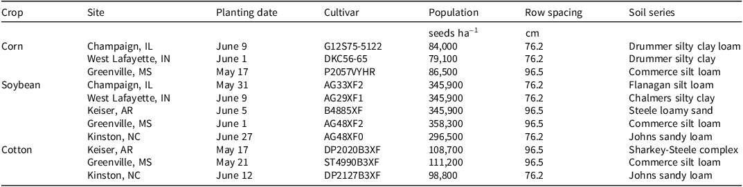
Each soybean and cotton experiment was planted with a glyphosate- and glufosinate-resistant cultivar at regionally recommended seeding rates in fields containing a natural population of weeds (Table 1). Corn hybrids were at least glyphosate-resistant and planted into natural weed populations at regionally recommended seeding rates. The corn experiments used labeled rates of S-metolachlor + atrazine + paraquat applied preemergence followed by (fb) atrazine + mesotrione + glyphosate + S-metolachlor applied postemergence (Table 2). The soybean herbicide program included S-metolachlor + metribuzin + paraquat applied preemergence fb glufosinate + S-metolachlor applied early postemergence fb glufosinate + acetochlor applied mid-postemergence. The cotton herbicide program was the same as the soybean program, with the exception being fluometuron rather than metribuzin was applied to cotton preemergence. Corn experiments did not have sequential postemergence applications, but soybean and cotton received mid-postemergence applications 14 d after early postemergence applications. All postemergence treatments also included a nonionic surfactant (Preference; Winfield United, Arden Hills, MN) at 0.25% (v/v). To indicate whether weeds were treated or not, postemergence-active herbicides included blue dye (Super Signal Blue; Precision Labs LLC, Kenosha, WI) at 0.25% (v/v). Cultural practices and soil information, including planting dates, soil series and textures, and row widths are listed in Table 1. All plots were 3.8 m wide and 29.5 m to 32.8 m long.
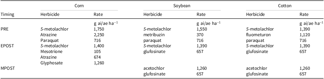
a Abbreviations: EPOST, early postemergence; MPOST, mid-postemergence; PRE, preemergence.
b Herbicide sources: Acetochlor, Warrant, Bayer Crop Science, St. Louis, MO; Atrazine, Atrazine 4L, Drexel Chemical Company, Memphis, TN; fluometuron, Cotoran 4L, ADAMA, Raleigh, NC; glufosinate, Noventa, BASF Corporation, Research Triangle Park, NC; glyphosate, Roudnup PowerMAX 3, Bayer Crop Science; mesotrione, Callisto, Syngenta Crop Protection, LLC, Greensboro, NC; metribuzin + S-metolachlor, Boundary 6.5 EC, Syngenta Crop Protection; S-metolachlor, Dual Magnum, Syngenta Crop Protection; paraquat, Gramoxone SL, Syngenta Crop Protection.
The sprayer used in the studies was previously described by Avent et al. (Reference Avent, Norsworthy, Patzoldt, Lazaro, Houston, Butts and Vazquez2024) as a dual-boom targeted sprayer engineered by Blue River Technology and was mounted to the front-end loader of a tractor. Ten nozzle bodies were spaced 38.1 cm apart. All herbicides were applied using the dual-boom system, which is capable of applying both broadcast and targeted applications in the same pass. At the preemergence application timing, broadcast treatments used PSLDMQ2003 nozzle tips (Deere & Company) calibrated to deliver 140 L ha−1 of water. Preemergence targeted herbicides were applied using SF4003 nozzles (Greenleaf Technologies, Covington, LA) calibrated to deliver 140 L ha−1 of water, and placed in a prototype cap that inclined the nozzle tip rearward at 30 degrees.
Postemergence treatments included the soil residual herbicides S-metolachlor or acetochlor applied through the broadcast boom with AIXR11002 nozzles (TeeJet Technologies, Glendale Heights, IL) calibrated to deliver 97 L ha−1 of water. In contrast, the foliar-active herbicides, glufosinate and mesotrione + atrazine + glyphosate, were sprayed through the targeted application boom. Glufosinate used in cotton and soybean experiments was applied with Deere & Company PS3DQ0004 nozzles all orientated toward the rearward position and calibrated to deliver 140 L ha−1 of water. Herbicides applied to corn, including mesotrione + atrazine + glyphosate, used Deere & Company PSLDMQ2003R4 nozzles all orientated to the rearward position and calibrated to deliver 140 L ha−1 of water.
Nozzles were selected based on droplet spectrum and characterization requirements for targeted applications (Gizotti de Moraes Reference Gizotti de Moraes2024). Broadcast treatments contained foliar-active and residual herbicides in the same tank and were applied using the same nozzles as the targeted herbicide applications, but in the standard configuration for broadcast applications (Supplementary Figure 1). For example, the PS3DQ0004 nozzles were alternated on the boom to create a twin-fan pattern, and the PSLDMQ2003 nozzles tips were orientated straight down. While the different nozzle orientations could affect spray particle coverage, the different orientations should not affect the ability to hit a weed (Ferguson et al. Reference Ferguson, Hewitt and O’Donnell2016).
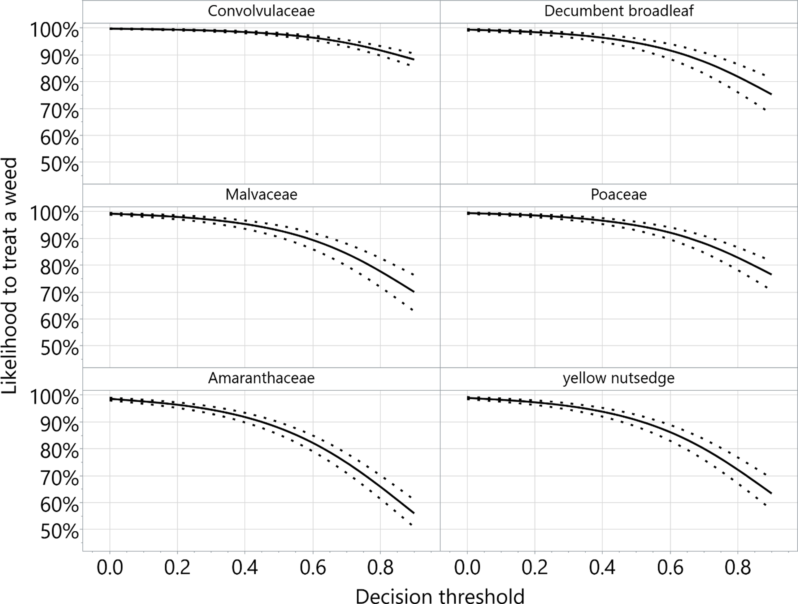
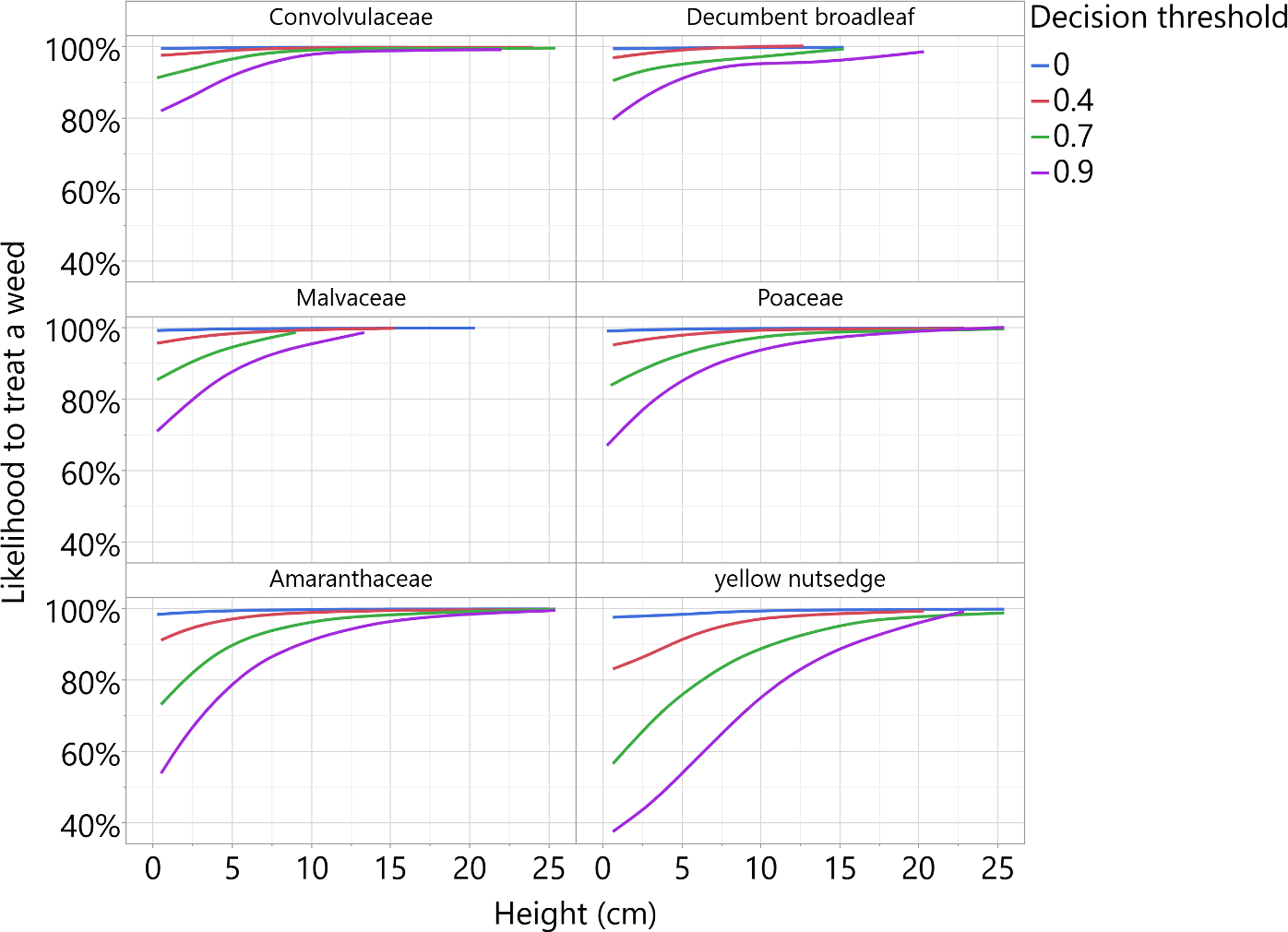
The effect of decision threshold on the likelihood of treating each weed class, averaged over the median height and width of each class, 2.4 plants m−2, and the categorical combination of between soybean rows. This figure should not be used to compare differences between weed classes due to differences between median weed height and width: Covolvulaceae, 3.8 cm and 5.1 cm; decumbent broadleaf, 1.3 cm and 1.3 cm; Malvaceae, 1.3 cm and 1.5 cm; Poaceae, 3.2 cm and 5.1 cm; Amaranthaceae, 1.9 cm and 2.5 cm; yellow nutsedge, 7.6 cm and 8.3 cm; respectively. Decision thresholds of 0.4, 0.7, and 0.9 correspond to the highest, medium, and lowest sensitivity settings in 2022, respectively. Broadcast applications are represented by 0. Average range odds ratio for decision threshold = 0.0192 (from broadcast to the lowest sensitivity). The solid lines represent the predicted likelihood to treat a weed, while the dotted lines represent the 95% confidence interval. Both lines were generated using the save columns function within the fit report of JMP Pro software (v. 18.0; SAS Institute, Cary, NC), with a smooth spline curve λ = 0.05.
Individual Plant Data
Before each postemergence herbicide application, weeds were marked with numbered wooden stakes in 3.3-m increments, traversing with the rows. Stakes were placed perpendicular to the direction of travel and at an angle to avoid blocking the camera view of each weed. Additionally, stake color (natural wood, orange, and red) was tested before application to ensure the stake did not trigger applications, and various sites used different colors. The goal was to mark at least 10 plants in the area; if 10 weeds did not occur within the first 3.3 m, an additional 3.3 m was marked. Areas of interest were only within the center furrow to avoid wheel tracks and could be as long as the entire plot (29.5 m to 32.8 m). Each weed was recorded for species, height, width, and position relative to the crop (in-row or between rows). The position of the weed was classified as “in-row” if the weed was within or beneath the crop canopy. Otherwise, it was denoted as “between rows.” The success of treating a weed was determined immediately after application by the presence or absence of blue dye on the plant: yes or no, respectively.
Data Preprocessing
A data column was created for each plot: the number of weeds was divided by the length of the area of interest to estimate weed density because some weeds could have been treated due to the presence of neighboring, larger weeds from multinozzle activation. Other predictors included crop (corn, cotton, or soybean), application timing, and sensitivity setting. In the results, the detection algorithm decision threshold will be referenced back to the 2022 sensitivity settings for clarity and consistency. A decision threshold set at zero was tested and confirmed that targeted applications would broadcast the entire area, so broadcast applications were zero for the decision threshold predictor. Lowest, medium, and highest sensitivity settings were set to the corresponding decision thresholds (0.9, 0.7, and 0.4, respectively). Continuous predictors included weed height, weed width, weed density, and decision threshold, while application timing, crop, weed aggregate class, and weed position relative to the crop were considered categorical predictors.
Across all sites and crops, 7,971 weeds were marked and recorded as treated or missed, but some species had too few observations to characterize the relationship or were never missed. The weeds with too few observations included common cocklebur (Xanthium strumarium L.), honeyvine swallowwort [Cynanchum laeve (Michx.) Pers.], Carolina horsenettle (Solanum carolinense L.), and sicklepod [Senna obtusifolia (L.) H.S. Irwin & Barneby]. All weeds >25.4 cm (height and width) were never missed or killed, so these observations were excluded. Weeds were aggregated into specific groups to preserve as many observations as possible (Table 3). All grasses were grouped into Poaceae. Three morningglory species were combined into Convolvulaceae. Palmer amaranth and waterhemp [Amaranthus tuberculatus (Moq.) J.D. Sauer] became Amaranthaceae. Yellow nutsedge (Cyperus esculentus L.) remained individually. Prickly sida (Sida spinosa L.) and velvetleaf (Abutilon theophrasti Medik) were combined to Malvaceae. Lastly, decumbent broadleaf weeds included carpetweed (Mollugo verticillata L.), curly dock (Rumex crispus L.), dandelion (Taraxacum officinale L.), horse purslane (Tranthema portulacastrum L.), and wild radish (Raphanus raphanistrum L.). A total of 21 different weeds were classified into six distinct groups. All other weeds were excluded from the analysis either because they did not occur in two or more experimental sites or they had never been missed. A total of 7,164 observations remained in the data set (Table 4).
Aggregate weeds and number, median height and width, and common name within each class after preprocessing the data set.a
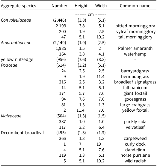
a Observations, heights, and widths in parenthesis correspond to the aggregate species.
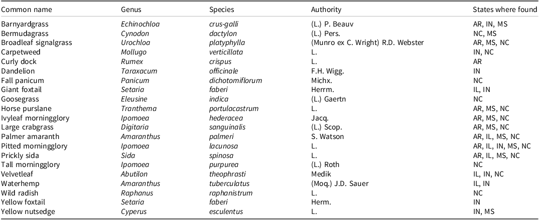
a Abbreviations: AR, Arkansas; IL, Illinois; IN, Indiana; MS, Mississippi; NC, North Carolina
b Names and authorities are from the WSSA composite list of weeds since not all names are present in the USDA plants database (https://wssa.net/weed/composite-list-of-weeds/)
Data Analysis
The analysis did not include the experimental site as a predictor to infer how targeted multinozzle applications performed across all locations. Additionally, application timing was not considered because this factor was implemented in the experimental design for whole-plot comparisons, and ultimately generated varying weed sizes and densities. Some weeds survived the early postemergence application and were present at mid-postemergence. These weeds were staked again for the sequential application, but injured weeds were not readily missed (visual observation). All other predictors were included in the analysis as one-way effects in the interest of parsimony. The response was a proportion of the weeds hit and is represented by ${p^h}$
, which ranges between 0 and 1. To link the proportion of treated weeds to the predictors, a logistic regression model (Eq. 1) was used,
${p^h}$
, which ranges between 0 and 1. To link the proportion of treated weeds to the predictors, a logistic regression model (Eq. 1) was used,
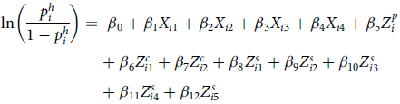 \begin{align}\ln \left( {{{p_i^h}}\over{{1 - p_i^h}}} \right) =& {\rm{\;}}{\beta _0} + {\beta _1}{X_{i1}} + {\beta _2}{X_{i2}} + {\beta _3}{X_{i3}} + {\beta _4}{X_{i4}} + {\beta _5}Z_i^p \\&+ {\beta _6}Z_{i1}^c + {\beta _7}Z_{i2}^c + {\beta _8}Z_{i1}^s + {\beta _9}Z_{i2}^s + {\beta _{10}}Z_{i3}^s \\&+ {\beta _{11}}Z_{i4}^s + {\beta _{12}}Z_{i5}^s\end{align}
where X i1, X i2, X i3, and X i4 is the ith observation of decision threshold, weed width, weed height, and weed density, respectively, with $i=1,\; \ldots, \;7,164$
. The variables
$i=1,\; \ldots, \;7,164$
. The variables $Z_i^p$
,
$Z_i^p$
, $Z_{ij}^c$
, and
$Z_{ij}^c$
, and $Z_{ij}^s$
are binary dummy variables corresponding to the categorical predictors of weed position, crop, and aggregated weed species, respectively. The variables are explained as follows:
$Z_{ij}^s$
are binary dummy variables corresponding to the categorical predictors of weed position, crop, and aggregated weed species, respectively. The variables are explained as follows:
- $Z_i^p=1$
if the weed position is in-row and 0 otherwise.
$Z_i^p=1$
if the weed position is in-row and 0 otherwise. -
$Z_{i1}^c=1$
if the crop is corn and 0 otherwise.
-
$Z_{i2}^c=1$
if the crop is cotton and 0 otherwise.
-
$Z_{i1}^s=1$
if the aggregated weed species is decumbent broadleaf and 0 otherwise.
-
$Z_{i2}^s=1$
if the aggregated weed species is Malvaceae and 0 otherwise.
-
$Z_{i3}^s=1$
if the aggregated weed species is Poaceae and 0 otherwise.
-
$Z_{i4}^s=1$
if the aggregated weed species is Amaranthaceae and 0 otherwise.
-
$Z_{i5}^s=1$
if the aggregated weed species is yellow nutsedge and 0 otherwise.


In Equation 1, ${\beta _j}$
is the coefficient of the jth predictor or dummy variable, which captures the average change in the log-odds to treat a weed (left-hand side of Equation 1) when the value of a predictor changes (James et al. Reference James, Witten, Hastie and Tibshirani2021; Menard Reference Menard2002). The estimation of the coefficients was calculated using the standard maximum likelihood estimation method.
${\beta _j}$
is the coefficient of the jth predictor or dummy variable, which captures the average change in the log-odds to treat a weed (left-hand side of Equation 1) when the value of a predictor changes (James et al. Reference James, Witten, Hastie and Tibshirani2021; Menard Reference Menard2002). The estimation of the coefficients was calculated using the standard maximum likelihood estimation method.
Likelihood ratio tests were used to measure the overall significance of the predictors (James et al. Reference James, Witten, Hastie and Tibshirani2021). A variable was deemed significant at α ≤ 0.05. Odds ratios with Wald tests were used for pairwise comparisons within the categorial predictors. Odds ratios are uncommon in weed science research (Menard Reference Menard2002). In layman’s terms, the odds of treating one scenario are compared to the odds of another scenario while holding all other predictors constant, and if the ratio has 95% confidence interval including 1, then the two scenarios are similar. A value of <1 indicates a reduction in the odds to treat a weed, while a value >1 indicates an increase. For continuous predictors, 95% confidence intervals were generated to visualize the estimated effects. The data analysis was performed using the fit model platform in JMP Pro software (v. 18.0; SAS Institute, Cary, NC) with a generalized regression personality.
Interpreting the Model
A range of responses are possible depending on the different predictors, and context is needed when stating a specific response in multivariate analyses. For clarity, predicted responses to aid in discussion will include specific scenarios that consider the other predictors and the median height and width of each species (Table 3). Equation 1 can be used in combination with the parameter estimates to calculate the likelihood of treating a weed (Supplementary Table 1). Figures were generated for each aggregate weed class using the median height and width of the specific weed class except when the figures use height or width as the independent variable. Additionally, the figures use the intercept for the categorical predictors, which are specific to between soybean rows.
Results and Discussion
Initial Observations
If weeds were always treated, there is no variance in the response, and the data do not provide a contribution to the analysis. Additionally, if there are too few observations, the parameter estimate is biased and may not accurately portray the relationship (Menard Reference Menard2002). Despite occurring in multiple sites, some weed species had to be excluded due to insufficient observational data, which caused biased estimates on the probability to treat weeds. Common cocklebur was never missed, with 52 observations. The other species that did not have enough data to determine the likelihood of treatment included honeyvine swallowwort, with three misses in 65 observations; Carolina horsenettle, with one miss in 41 observations; and sicklepod, with two misses in 27 observations. Unfortunately, there were insufficient observations for these species, resulting in biased parameter estimates and the need to be excluded.
Based on the likelihood ratio tests, the most significant predictor for treating a weed was the decision threshold (Table 5), with a likelihood ratio χ2 = 750.5. In order of importance, other significant predictors included aggregate weed species, weed width, weed position (in-row or between rows), and weed height. Weed density and the crop were not significant according to the likelihood ratio tests, and did not influence the likelihood of treating a weed. Decision threshold (sensitivity setting) is the most important predictor, which is unsurprising because this setting dictates that weeds are classified as such. The weed width also appears to drive the predictions more than height, which is likely due to the orientation of the cameras being angled downward and collinearity between weed height and width (r = 0.727). The decision to leave height and width in the model despite collinearity is due to the width being more relevant for the detection algorithm. However, height is more practical for operators who measure height, not width, before herbicide applications.
Likelihood ratio effect summary for the logistic regression of treated weeds.a

a Abbreviation: DF, degrees of freedom.
Differences among Aggregate Species, Weed Position, and Crop to Treat Weeds
Targeted applications (across sensitivity settings, median weed height and width, and density of 2.4 plants m−2) resulted in a treatment success of 99.6% to 84.4% for Convolvulaceae, 99.1% to 68.8% for decumbent broadleaf weeds, 98.9% to 62.9% for Malvaceae, 99.1% to 70.3% for Poaceae, 98.0% to 48.3% for Amaranthaceae, and 98.5% to 55.8% for yellow nutsedge (data not shown). On average, Convolvulaceae and decumbent broadleaf weeds were among the easiest to target (Table 6). These two aggregate classes would have a high groundcover percentage (Bryson and DeFelice Reference Bryson and DeFelice2009), presumably because they are easier to detect with downward-oriented cameras (Lazaro et al. Reference Lazaro, Houston and Patzoldt2024). Yellow nutsedge was more difficult to control than all other aggregate species when using comparable sensitivity settings, which is unsurprising due to the plant’s thin leaves and upright architecture (Bryson and DeFelice Reference Bryson and DeFelice2009), which suggests different machine settings would be required to increase the probability of treating this species. Alternatively, those who apply herbicides could consider broadcasting an effective foliar-active herbicide along with targeted applications to improve control of specific species such as yellow nutsedge.
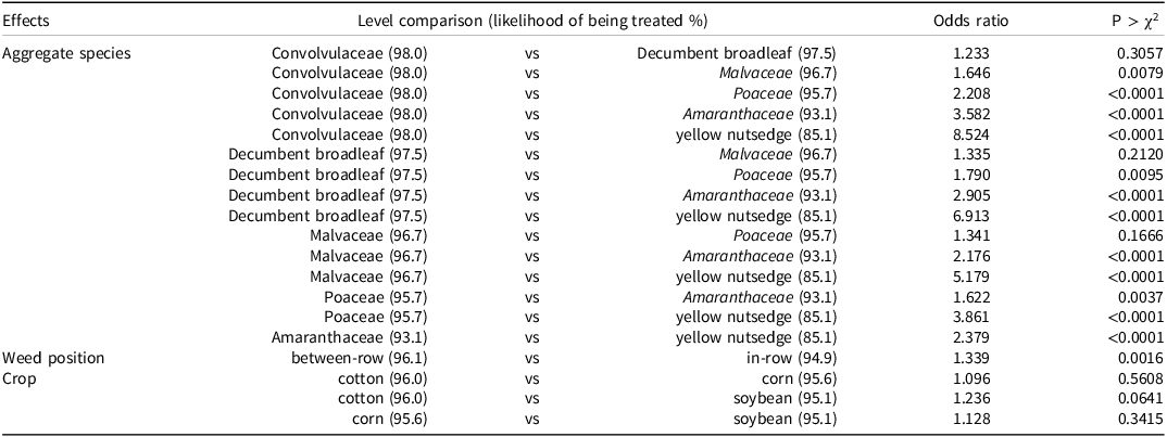
a Odds ratios are calculated from the ratio of the two levels: ${{\left( {{{{P_a}}}\over{{1 - {P_a}}}} \right)}}\over{{\left( {{{{P_b}}}\over{{1 - {P_b}}}} \right)}}$
where P a is the proportion of the treated weeds for one group and P b is the proportion of treated weeds for the comparison group. As an example, if P a = 0.9 and P b = 0.8, the odds ratio would be
${{\left( {{{{P_a}}}\over{{1 - {P_a}}}} \right)}}\over{{\left( {{{{P_b}}}\over{{1 - {P_b}}}} \right)}}$
where P a is the proportion of the treated weeds for one group and P b is the proportion of treated weeds for the comparison group. As an example, if P a = 0.9 and P b = 0.8, the odds ratio would be ${{{\left( {{{0.9}}\over{{1 - 0.9}}} \right)}}\over{{\left( {{{0.8}}\over{{1 - 0.8}}} \right)}}}=2.25$
. Likelihoods parenthetically presented represent the likelihood averaged over all other predictors.
${{{\left( {{{0.9}}\over{{1 - 0.9}}} \right)}}\over{{\left( {{{0.8}}\over{{1 - 0.8}}} \right)}}}=2.25$
. Likelihoods parenthetically presented represent the likelihood averaged over all other predictors.
b P > χ2 are Wald-based tests from the model estimates.
Some species may require special attention when considering settings to target-apply herbicides, such as those from the Amaranthus genus. There have been many reports that Palmer amaranth and waterhemp are developing herbicide resistance (Carvalho-Moore et al. Reference Carvalho-Moore, Norsworthy, González-Torralva, Hwang, Patel, Barber, Butts and McElroy2022; Evans et al. Reference Evans, Strom, Riechers, Davis, Tranel and Hager2019; Foster and Steckel Reference Foster and Steckel2022; Heap Reference Heap2024; Randell-Singleton et al. Reference Randell-Singleton, Hand, Vance, Wright-Smith and Culpepper2024). Other research has also demonstrated that young waterhemp and Palmer amaranth plants can grow up to 16.8 and 29 cm per week, respectively (Heneghan and Johnson Reference Heneghan and Johnson2017; Spaunhorst et al. Reference Spaunhorst, Devkota, Johnson, Smeda, Meyer and Norsworthy2018). Operators who use targeted applications cannot afford to miss small Amaranthus species, which could be uncontrollable within a week after application.
Regarding weed position, odds ratios indicated that weeds were more easily treated between rows (96.1%) versus within the crop rows (94.9%), averaged over all other predictors (Table 6). The higher success rate for treating weeds between rows was expected because weed occlusion by intermingling plant parts has already been reported by Franz et al. (Reference Franz, Gebhardt and Unklesbay1991) and herbicide coverage by Creech et al. (Reference Creech, Henry, Hewitt and Kruger2018). However, herbicides used in this research were applied while the machine traversed with the rows, rather than at an angle against the rows. The results could be more severe if herbicides are applied at an angle, which could more readily occlude weeds. Additionally, the lack of differences between the three crops evaluated in this study indicates that the different detection algorithms performed similarly.
Differences in Treating Weeds among Sensitivity Settings, Weed Size, and Weed Densit
To reiterate, the continuous decision thresholds of 0.4, 0.7, and 0.9 corresponded to the highest, medium, and lowest spray sensitivities in 2022, respectively. Broadcast applications were set at a threshold of zero, and applications at this setting confirmed uniform deposition across the area (100% area sprayed). Figure 1 uses the median height and width of each aggregate weed class to present a visualization of the decision threshold and is not intended to compare the different weed classes. On average, the range odds ratio (probability of a hit at 0 versus the probability of a hit at 0.9) is 0.0192 for the range of decision thresholds, indicating a decrease in the odds to treat a weed with decreasing sensitivity levels. Interestingly, the standard error for the likelihood to treat a weed also increased with the decision threshold from 0 to 0.9. The increase in the standard error demonstrates the uncertainty associated with changes in the sensitivity setting.
The fact that lower sensitivity settings (increasing decision thresholds) reduces the ability to treat weeds is concerning since producers will be inclined to reduce the area they spray both to reduce the amount of herbicides they use and thus save money, or to implement herbicide mitigation efforts outlined by the U.S. Environmental Protection Agency’s Herbicide Strategy (US EPA 2024). However, understanding these dynamics coupled with weed sizes can broaden the utility of targeted applications. If operators intend to mimic a broadcast treatment with targeted applications, the highest sensitivity setting (decision threshold 0.4) could maximize weed control success with targeted multinozzle applications. Alternatively, the low sensitivity setting (decision threshold 0.9) is not intended for typical applications. The low sensitivity setting makes the most sense when producers want to target only large weeds; examples include 1) when volunteer crops appear, 2) when dual-boom applications are used at a standard rate in the broadcast tank and the targeted tank contains a spiking dose, and 3) when multiple herbicides are applied, where one is broadcasted for small weeds and targeted herbicides are used to control larger weeds (e.g., glufosinate broadcast and 2,4-D targeted, or atrazine broadcast and mesotrione targeted). Future research should evaluate the efficacy and economics of these scenarios to aid in the utility of targeted sprayers.
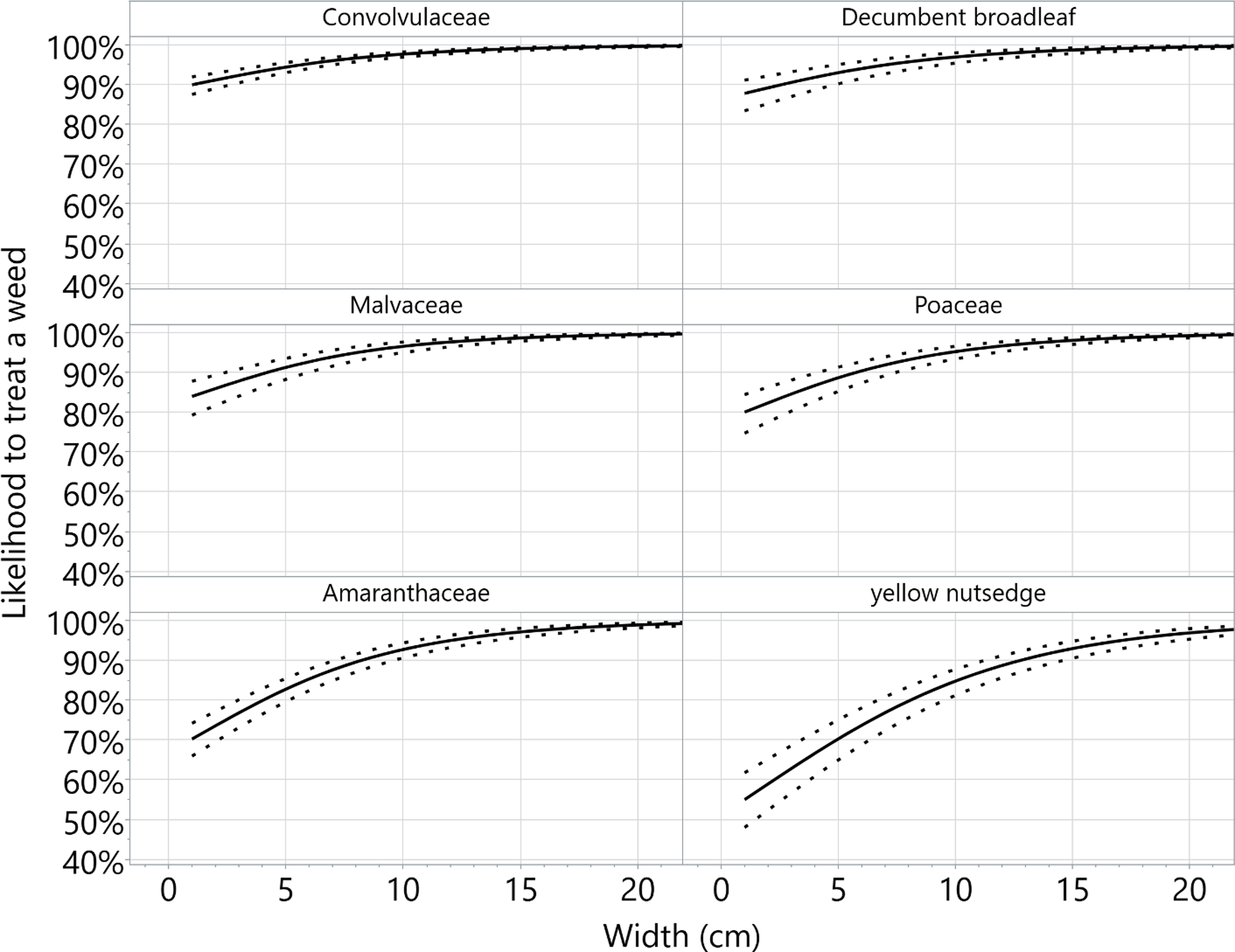
Both weed height and width positively influenced the ability to treat weeds with targeted applications (Figures 2 and 3). Averaged over all other predictors, both height and width had unit odds ratios (1 cm increments) of 1.07 and 1.15, respectively, meaning increases in either predictor result in increasing the odds to treat a weed. One of the primary limitations of a one-way analysis is not being able to ascertain the effects in combination with other main effects. However, when considering the Amaranthaceae aggregate class at an averaged medium spray sensitivity (decision threshold 0.7) and weed density of 2.4 plants m−2, the probability of treating a 2.5-cm plant (height and width) was 0.69 to 0.84 based on 95% confidence intervals. Increasing the same weed size to 5 cm resulted in likelihoods to treat from 0.75 to 0.87 based on 95% confidence. Additionally, since width appears to drive the likelihood of treating weeds over height (Table 5), scouting practices prior to targeted herbicide applications should consider weed width when providing recommendations on the selection of sensitivity settings to achieve a desired result. However, this information would be in addition to plant height, which is the primary consideration for herbicide product labels.
The effect of weed height (in centimeters) on the likelihood of treating a weed with targeted applications, at a 0.7 decision threshold (medium sensitivity) and the categorical combination of between soybean rows. Average unit odds ratio for width = 1.065. Solid lines represent the predicted likelihood to treat a weed, while the dotted lines represent the 95% confidence interval. Both lines were generated using the save columns function within the fit report of JMP Pro software (v. 18.0; SAS Institute, Cary, NC), with a smooth spline curve λ = 0.05.

The effect of weed width (in centimeters) on the likelihood of treating each weed class at a medium sensitivity setting (decision threshold 0.7) and the categorical combination of between soybean rows. Unit odds ratio for width = 1.150. Solid lines represent the predicted likelihood to treat a weed, while the dotted lines represent the 95% confidence interval. Both lines were generated using the save columns function within the fit report of JMP Pro software (v. 18.0; SAS Institute, Cary, NC), with a smooth spline curve λ = 0.05.
When considering the combination of sensitivity setting, weed size, and weed species, the herbicide being applied also requires consideration. For example, field applications of glufosinate formulations require a minimum of 7, 10, and 5 d between sequential applications to corn, cotton, and soybean, respectively (Anonymous 2023). In addition to the reapplication restriction, if producers are applying a sequential postemergence herbicide, the general recommendation is to apply 14 d later (Barber et al. Reference Barber, Scott, Wright-Smith, Jones, Norsworthy, Burgos and Bertucci2025). If weeds are missed while they are small, some could grow rapidly between sequential applications, and weeds larger than 8 cm would likely be poorly controlled (Priess et al. Reference Priess, Popp, Norsworthy, Mauromoustakos, Roberts and Butts2022). Therefore, when treating small weeds, operators should use a higher sensitivity setting (lower decision threshold) to maximize herbicide coverage and weed control, which provided 91.1% likelihood to treat Amaranthaceae weeds that were 2.5 cm tall and wide between soybean rows. The same scenario, but changed to a medium or lowest sensitivity setting, treated Amaranthaceae weeds 73.3% and 53.2% of the time, respectively.
Previous research has indicated that high weed densities could affect the ability of machine vision technologies to detect weeds among crops (El Jgham et al. Reference El Jgham, Abdoun, El Khatir, Kacprzyk, Ezziyyani and Balas2023; Franz et al. Reference Franz, Gebhardt and Unklesbay1991). However, based on the results from this analysis, density did not appear to affect the likelihood of treating weeds (Table 5; Figure 4). Even if some weeds were occluded, targeted, multinozzle applications appeared to compensate by treating adjacent, detected weeds. However, this experiment did not directly evaluate detection performance or quantify spray coverage across the swath of activated nozzles. Other research simulating nozzle density when treating turfgrass demonstrated that a lower nozzle density (i.e., wider nozzle spacings) generated a higher number of false hits, meaning areas where weeds were undetected were sprayed (Petelewicz et al. Reference Petelewicz, Zhou, Schiavon, MacDonald, Schumann and Boyd2024). In this research, targeted applications occurred through multinozzle activation with ≥100-degree nozzles (Gizotti de Moraes Reference Gizotti de Moraes2024), which likely inflated the likelihood of treating weeds through so-called false hits. Weeds may have been present and adjacent to detectable weeds, but they were not actually detected by the machine vision algorithm. Narrower nozzle angles or single nozzle–activating systems could increase the likelihood of missing weeds, and further research is needed to evaluate these concerns and quantify spray deposition at the edge of activated tapered nozzles.
Effect of weed density (plants per square meter) on the likelihood of treating yellow nutsedge between soybean rows. The figure also uses the medium sensitivity setting (decision threshold 0.7) and the median yellow nutsedge height and width at 7.6 cm and 8.3 cm, respectively. The unit odds ratio for weed density = 0.989 and was insignificant. The solid lines represent the predicted likelihood to treat a weed, while the dotted lines represent the 95% confidence interval. Both lines were generated using the save columns function within the fit report of JMP Pro software (v. 18.0; SAS Institute, Cary, NC), with a smooth spline curve λ = 0.05.

Overall, if an operator treats a field of weeds that are small or difficult to detect, spray sensitivities should be higher to maximize detection and targeted application success. Currently, the user interface displays a scale from lowest to highest spray sensitivity and does not provide any metric on the likelihood or actual weed size or the decision threshold (Anonymous 2024). An alternative solution could be to use data from these experiments and allow the operator to select a weed size (height or width), allowing the threshold to change to a setting that achieves >0.90 probability of treating a specific weed class. However, one limitation of this analysis is the inability to assess specific crop and weed interactions. Future research should explore the effects of certain weed species within individual crops. Another consideration is that model updates are and will be continuous in the future, which means performance results may vary among model releases. Lastly, this research investigating targeted applications was conducted with a specific technology. Other systems that utilize individually activated, even-fan nozzles may perform differently than the technology evaluated here due to differing machine vision algorithms, sprayer speeds, nozzle orientations, etc.
Practical Implications
The research described here highlights the ability of targeted applications of herbicides to treat problematic weed species. Small weeds will always be difficult to detect and treat regardless of the detection system since successful targeted applications depend on both the ability to detect and apply herbicides. Even broadcast applications of herbicides to eliminate small weeds can provide inadequate droplet coverage with some combinations of nozzle tips and carrier volumes (Hassen et al. Reference Hassen, Sidik and Sheriff2013). Regardless, continued advancements and improvements in targeted spray technology, such as camera resolution, boom stability, and detection algorithms, should improve the ability to manage small weeds. Our results also indicate that weed position (between or in-row) and the subsequent occlusion of weeds did influence the ability to spray weeds with targeted applications. These data highlight which aggregate species are problematic and allow targeted collection efforts to improve the training data set used to develop the detection algorithm (Figure 5). Additionally, the John Deere company has made updates to the system since 2022, and these results may underestimate current system performance.
The observed likelihood of treating each aggregate group of weeds given the weed height (in centimeters) and decision thresholds across observations. Decision thresholds of 0.4, 0.7, and 0.9 correspond to the highest, medium, and lowest spray sensitivities settings in 2022, respectively. Broadcast applications are represented by 0. The figure was generated using the graph builder platform with JMP Pro software (v. 18.0; SAS Institute, Cary, NC) with a smooth spline line with λ = 8.5.
Currently, producers or herbicide equipment operators do not know the decision threshold that corresponds to the spray sensitivity level options in the sprayer display. The corresponding decision thresholds are also subject to change based on performance or savings from internal testing in each year. More transparency is needed to allow operators to make an informed decision when selecting the sensitivity level for a targeted herbicide application. Otherwise, failures could occur more frequently, or additional applications may be needed to adequately control problematic weed species. However, the data we collected across all experimental sites could be used to optimize the applicator settings.
Supplementary material
To view supplementary material for this article, please visit https://doi.org/10.1017/wet.2025.36
Acknowledgments
We thank the many support staff personnel at the experiment stations where this research was conducted. We also thank the many fellow graduate students, interns, and research associates who invested long hours in carrying out this research. Without their help and support, these trials would have been infeasible.
Funding
Funding for this research, the agronomy testing machine, and technical support for the system were provided by Blue River Technology and Deere & Company.
Competing Interests
Authors William Patzoldt, Lauren Schwartz-Lazaro, and Michael Houston are employees of Blue River Technology. The other authors are employed by various universities and declare they have no conflicting interests.


 Open access