3.1. An illustrative example

Consider the following analytical model taken from Forrester, Sóbester & Keane (Reference Forrester, Sóbester and Keane2007) to generate HF and LF samples of the QoI $y$ for input $x\in [0,1]$:

(3.1)\begin{equation} \left.\begin{array}{c} y_{H}(x)=(\theta x-2)^2 \sin (2\theta x-4) \\ y_{L}(x)=y_{H}(x) + B(x-0.5)-C \end{array}\right\} . \end{equation}

In Forrester et al. (Reference Forrester, Sóbester and Keane2007), $\theta$ is taken to be fixed and equal to $6$, but here it is treated as an uncertain calibration parameter that is to be estimated during the construction of the MFM. Note that the notations of the general model (2.5) can be adopted for (3.1). For simulator $\hat {f}(x,t)$ and model discrepancy $\hat {\delta }(x)$ the covariance matrix in (2.8) is used with the exponentiated quadratic kernel (2.11). The following prior distributions are considered: $\lambda _f, \lambda _\delta \sim \mathcal {HC}(\alpha =5)$, $\ell _{f_x}, \ell _{f_t}, \ell _{\delta _x} \sim \varGamma (\alpha =1,\beta =5)$, $\varepsilon \sim \mathcal {N}(0,\sigma )$ with $\sigma \sim \mathcal {HC}(\alpha =5)$ and $\theta \sim \mathcal {U}[5.8,6.2]$. Here, $\mathcal {HC}, \varGamma, \mathcal {N}$ and $\mathcal {U}$ denote the half-Cauchy, gamma, Gaussian, and uniform distributions, respectively, see table 2. The HF training samples are taken at $x=\{0,0.4,0.6,1\}$, therefore, $n_H=4$ is fixed. To investigate the effect of $n_L$, three sets of LF samples of size $10, 15$ and $20$ are considered which are generated by Latin hypercube sampling from the admissible space $[0,1]\times [5.8,6.2]$ corresponding to $x$ and $t$ (uncalibrated instance of $\theta$), respectively.

Using the data, the HC-MFM (2.6) for problem (3.1) is constructed. The first row in figure 2 shows the predicted $y$ with the associated $95\,\%$ confidence interval (CI) along with the training data and reference true data generated with $\theta =6$. For all $n_L$, the predicted $y$ is closer to HF data than the LF data, however, for $n_L=15$ and $20$, the agreement between the mean of the predicted $y$ and the true data is significantly improved. A better validation can be made via the plots in the second row of figure 2, where the predicted $y$ and true values of $y_H$ at $50$ uniformly spaced test samples for $x\in [0,1]$ are plotted. Clearly, increasing the number of the LF samples while keeping $n_H=4$ fixed improves the predictions and reduces the uncertainty. In the third row of figure 2, the posterior densities of $\theta$ are presented. In all cases, a uniform (non-informative) prior distribution over $[5.8,6.2]$ was considered for $\theta$. Only for $n_L=20$, the resulting posterior density of $\theta$ is high near the true value $6$. Therefore, it is confirmed that, as explained by Goh et al. (Reference Goh, Bingham, Holloway, Grosskopf, Kuranz and Rutter2013), the main capability of the HC-MFM (2.6) is in making accurate predictions for $y$ and only if a sufficient number of training data are available, accurate distributions for the calibration parameters are also obtained. This is shown here by fixing $n_H$ and increasing $n_L$, which is favourable in practice. It is also noteworthy that if $\theta$ was known and hence treated as a fixed parameter, then even with $n_L=10$ very accurate predictions for $y$ could be already achieved (not shown here).

Figure 2.

(a–c) Predicted QoI $y$ by HC-MFM (2.6) along with the training and true data, (d–f) predicted $y$ vs true observations at $50$ test samples of $x\in [0,1]$ with error bars representing $95\,\%$ CI, (g–i) posterior probability density function (PDF) of $\theta$ based on $10^4$ MCMC samples. The $y_H$ and $y_L$ training data are generated from (3.1) using $B=C=10$. The training data include $4$ HF samples combined with (left column) $10$, (middle column) $15$ and (right column) $20$ LF samples. The true data are generated by (3.1) using $\theta =6$.

It also should be noted that the mean of the posterior distribution of $\sigma$, the noise standard deviation, is found to be negligible, as expected. This is in fact the case for all other examples in this section.

3.2. Turbulent channel flow

Turbulent channel flow is one of the most canonical wall-bounded turbulent flows. The flow develops between two parallel flat walls which are apart by the distance $2\delta$, and the flow is periodic in the streamwise and spanwise directions. Channel flow is fully defined by a Reynolds number, for instance the bulk Reynolds number $Re_b=U_b\delta /\nu$, where $U_b$ and $\nu$ specify the streamwise bulk velocity and kinematic viscosity, respectively. Among different possible QoIs, here we only focus on the friction velocity $\langle u_\tau \rangle$, as a function of Reynolds number. This quantity is defined as $\sqrt {\langle \tau _w \rangle /\rho }$, where $\tau _w$ and $\rho$ are the magnitude of the wall-shear stress and fluid density, respectively, and $\langle {\cdot } \rangle$ represents averaging over time and the periodic directions. Three fidelity levels are considered: DNS ($M_1$), wall-resolved LES (WRLES) ($M_2$) and a reduced-order algebraic model ($M_3$), where the fidelity reduces from the former to the latter. We use the DNS data of Iwamoto, Suzuki & Kasagi (Reference Iwamoto, Suzuki and Kasagi2002), Lee & Moser (Reference Lee and Moser2015) and Yamamoto & Tsuji (Reference Yamamoto and Tsuji2018).

The WRLES of channel flow have been performed at different Reynolds numbers without any explicit subgrid-scale model using OpenFOAM (Weller et al. Reference Weller, Tabor, Jasak and Fureby1998), which is an open-source finite-volume flow solver. Linear interpolation is used for the evaluation of face fluxes, and a second-order backward-differencing scheme is used for time integration. The pressure-implicit with splitting of operators (PISO) algorithm is used for pressure–velocity coupling. For further details on the simulation set-up, see Rezaeiravesh & Liefvendahl (Reference Rezaeiravesh and Liefvendahl2018). The results in that paper show that for a fixed resolution in the wall-normal direction, variation of the grid resolutions in the wall-parallel directions could significantly impact the accuracy of the flow QoIs. Therefore, in the context of the HC-MFM, the calibration parameters for WRLES are taken to be ${{\rm \Delta} x^+}$ and ${{\rm \Delta} z^+}$, which are the cell dimensions in the streamwise and spanwise directions, respectively, expressed in wall units (${{\rm \Delta} x^+}={\rm \Delta} x u^\circ _\tau /\nu$ where $u^\circ _\tau$ is the reference $u_\tau$ from DNS).

At the lowest fidelity, the following reduced-order algebraic model is considered which is derived by averaging the streamwise momentum equation for the channel flow in the periodic directions and time:

(3.2)\begin{equation} \langle u_\tau \rangle^2/U_b^2=\frac{1}{Re_b} \frac{\mbox{d}}{\mbox{d} \eta} \left( (1+\zeta(\eta)) \frac{\mbox{d}\langle u \rangle/U_b}{\mbox{d} \eta} \right) , \end{equation}

where $\eta$ is the distance from the wall normalized by the channel half-height $\delta$, and $\zeta (\eta )$ is the normalized eddy viscosity $\nu _t$, i.e. $\zeta (\eta )=\nu _t(\eta )/\nu$. Reynolds & Tiederman (Reference Reynolds and Tiederman1967) proposed the following closed form for $\zeta (\eta )$:

(3.3)\begin{align} \zeta(\eta) =\frac{1}{2} \left[1+\frac{{\kappa}^2 Re^2_\tau}{9}(1- (\eta-1)^2)^2 (1+2(\eta-1)^2)^2 \left(1-\exp\left(\frac{-\eta Re_\tau}{A^+}\right) \right)^2 \right]^{1/2} \!\!-\frac{1}{2} , \end{align}

where ${Re}_\tau =\langle u_\tau \rangle \delta /\nu$ is the friction-based Reynolds number, and $\kappa$ and $A^+$ are two modelling parameters. At any ${Re}_b$ (and given value of $\kappa$ and $A^+$), (3.2) is integrated over $\eta \in [0,1]$ and is iteratively solved using (3.3) to estimate $\langle u_\tau \rangle$. Expressing the channel flow example in the terminology of MFM (2.6), $\langle u_\tau \rangle /U_b$ is the QoI $y$, $x=Re_b$, $\boldsymbol {t}_3=(\kappa,A^+)$ and $\boldsymbol {t}_2=({{\rm \Delta} x^+},{{\rm \Delta} z^+})$. The training data set consists of the following databases. For DNS, $\langle u_\tau \rangle$ is taken from Iwamoto et al. (Reference Iwamoto, Suzuki and Kasagi2002), Lee & Moser (Reference Lee and Moser2015) and Yamamoto & Tsuji (Reference Yamamoto and Tsuji2018) at $Re_b=5020$, $6962$, $10\ 000$, $20\ 000$, $125\ 000$ and $200\ 400$. In total, $16$ WRLES $\langle u_\tau \rangle$ samples are obtained from a design of experiment based on the prior distributions ${{\rm \Delta} x^+}\sim \mathcal {U}[15,85]$ and ${{\rm \Delta} z^+}\sim \mathcal {U}[9.5,22]$ at ${Re}_b=5020,6962,10\ 000$, and $20\ 000$. Here, we do not consider the observational uncertainty in $\langle u_\tau \rangle$ which could, for instance, be due to finite time averaging in DNS and WRLES, but in general the HC-MFM could take such information into account. The reduced-order model (3.2) which is computationally cheap is run for $10$ values of ${Re}_b$ in range $[2000,200\ 200]$. For each ${Re}_b, 9$ joint samples of $(\kappa,A^+)$ are generated assuming $\kappa \sim \mathcal {U}[0.36,0.43]$ and $A^+\sim \mathcal {U}[26.5,29]$ (note that $\kappa$ is the von Kármán coefficient). For all the GPs in the MFM (2.6), the exponentiated quadratic covariance function (2.11) is used. The prior distribution of the hyperparameters are set as the following: $\lambda _f, \lambda _g \sim \mathcal {HC}(\alpha =5)$, $\lambda _{\delta } \sim \mathcal {HC}(\alpha =3)$, $\ell _{f_x}, \ell _{f_{t_3}},\ell _{g_x}, \ell _{g_{t_2}}, \ell _{\delta _x} \sim \varGamma (\alpha =1,\beta =5)$ and the noise standard deviation $\sigma \sim \mathcal {HC}(\alpha =5)$ (assumed to be the same for all fidelities).

Using the described training data in the HC-MFM (2.6) and running the MCMC chain for $7000$ samples, after an initial $2000$ samples discarded due to burn in, the model is constructed. This means extra MCMC samples are generated from which a sufficiently large number of initial samples is discarded to avoid any bias introduced by the initialization. According to figure 3(a), the predicted mean of $\langle u_\tau \rangle /U_b$ follows the trend of the DNS data. This approximately holds even at high Reynolds numbers, where there is a large systematic error in the algebraic model and no WRLES data are available. As expected, in this range due to scarcity of the DNS data, the uncertainty in the predictions is high. The plot in figure 3(b) shows the joint posterior distributions of the calibration parameters $\kappa, A^+, {{\rm \Delta} x^+}$ and ${{\rm \Delta} z^+}$ along with the histogram of each parameter. As mentioned above, the prior distributions of all of these parameters were assumed to be uniform and mutually independent. However, the resulting posterior densities for $\kappa$ and $A^+$ are not uniform and the samples of these parameters are correlated. More interestingly, the peak of the posterior density of $\kappa$ is close to the value of $0.4$ that is assumed to be universal across various flows and Reynolds numbers within the turbulence community. On the other hand, the distribution of $A^+$ does not show a clear maximum, which may indicate that the range of admissible values in the prior could be extended. Note that indeed the value of $A^+=25$ is associated with the van-Driest wall damping commonly used for eddy-viscosity models. In contrast, the posteriors of ${{\rm \Delta} x^+}$ and ${{\rm \Delta} z^+}$ are found to be still close to the prior uniform distributions and no correlation between their samples is observed. This may be at least partially be due to the fact that the number of the WRLES data is limited as they are obtained only at 4 Reynolds numbers. Nevertheless, over this range of the Reynolds number the posterior prediction of the QoI $\langle u_\tau \rangle$ is very accurate and has the lowest uncertainty, which seems to indicate that the significant dependence of the wall-shear stress on the WRLES resolution did not lead to a bias in the prediction by the HC-MFM. This may in fact be an important aspect for building future wall models.

Figure 3.

(a) Mean prediction of $\langle u_\tau \rangle /U_b$ and associated $95\,\%$ CI along with the training data and validation data from DNS of Iwamoto et al. (Reference Iwamoto, Suzuki and Kasagi2002), Lee & Moser (Reference Lee and Moser2015) and Yamamoto & Tsuji (Reference Yamamoto and Tsuji2018), (b) diagonal, posterior density of parameters $\kappa, A^+, {{\rm \Delta} x^+}$ and ${{\rm \Delta} z^+}$; off diagonal, contour lines of the joint posterior densities of these parameters. The value of the contour lines increases from the lightest to darkest colour.

3.3. Polars for the NACA0015 airfoil

In this section, the HC-MFM (2.6) is applied to a set of data for the lift and drag coefficients, $C_L$ and $C_D$, respectively, of a wing with a NACA0015 airfoil profile at Reynolds number $1.6\times 10^6$. The angle of attack (AoA) between the wing and the ambient flow is taken to be the design parameter $x$.

The data consist of the following sources with respective fidelities in brackets: wind-tunnel experiments by Bertagnolio (Reference Bertagnolio2008) ($M_1$), detached-eddy simulations (DES) ($M2$) and two-dimensional RANS ($M_3$) both by Gilling, Sørensen & Davidson (Reference Gilling, Sørensen and Davidson2009). The simulations of Gilling et al. (Reference Gilling, Sørensen and Davidson2009) were performed with a finite-volume code using a fourth-order central-difference scheme and a second-order accurate dual time-stepping algorithm to integrate the momentum equations. The PISO algorithm was used to enforce pressure–velocity coupling. In the study, the authors investigated the sensitivity of the DES results to the resolved turbulence intensity (TI) of the fluctuations imposed at the inlet boundary. The sensitivity was found to be particularly significant near the stall angle. Therefore, when constructing an MFM, the calibration parameter $t_2$ in fidelity $M_2$ is taken to be the TI.

For the covariance of the Gaussian processes $\hat {f}(x)$ and $\hat {g}(x,t_2)$ in HC-MFM (2.6), the exponentiated quadratic and Matern-5/2 kernel functions (2.11) and (2.12) are used, respectively. The following prior distributions are assumed for the hyperparameters: $\lambda _f , \lambda _g \sim \mathcal {HC}(\alpha =5)$, $\ell _{f_x}\sim \varGamma (\alpha =1,\beta =5)$, $\ell _{g_x},\ell _{g_{t_2}}\sim \varGamma (\alpha =1,\beta =3)$ and the noise standard deviation $\sigma \sim \mathcal {HC}(\alpha =5)$ (assumed to be the same for all fidelities). To make the model capable of capturing large-scale separation, the stall AoA, $x_{stall}$, is included as a new calibration parameter in the MFM. Our suggestion is to consider a piecewise kernel function for the covariance of $\hat {\delta }(x)$ where $x_{stall}$ is the merging point. If the kernel functions for the AoAs smaller and larger than $x_{stall}$ are denoted by $k_{\delta _1}({\cdot })$ and $k_{\delta _2}({\cdot })$, respectively, then the covariance function for $\hat {\delta }(x)$ may be constructed as

(3.4)\begin{equation} \varSigma_{\delta_{ij}} = \lambda_{\delta_1}^2 \varphi(x_i) k_{\delta_1}(\bar{d}_{\delta_{ij}}) \varphi(x_j) + \lambda_{\delta_2}^2 \varphi(x_i) k_{\delta_2}(\bar{d}_{\delta_{ij}}) \varphi(x_j), \end{equation}

where $\bar {d}_{\delta _{ij}}$ is defined similar to those in (2.9) and (2.10) but only in $x$, and $\varphi (x)$ is a function to smoothly merge the two covariance functions. In particular, we use the logistic function:

(3.5)\begin{equation} \varphi(x)=[1+\exp(-\alpha_{stall}(x-x_{stall}))]^{-1} , \end{equation}

where $\alpha _{stall}$ is a new hyperparameter. The kernel functions $k_{\delta _1}({\cdot })$ and $k_{\delta _2}({\cdot })$ are both modelled by the Matern-5/2 function (2.12). As the prior distributions, we assume $\lambda _{\delta _1}\sim \mathcal {HC}(\alpha =3)$, $\lambda _{\delta _2}\sim \mathcal {HC}(\alpha =5)$, $\ell _{\delta _1}\sim \varGamma (\alpha =1,\beta =5)$, $\ell _{\delta _2}\sim \varGamma (\alpha =1,\beta =0.5)$, $\alpha _{stall}\sim \mathcal {HC}(\alpha =2)$ and $x_{stall}\sim \mathcal {N}(14,0.2)$. The prior for the TI is also considered to be Gaussian: ${TI}\sim \mathcal {N}(0.5,0.15)$. These Gaussian priors are selected based on our prior knowledge about the approximate stall AoA and the discussion about the influence of TI in Gilling et al. (Reference Gilling, Sørensen and Davidson2009).

The admissible range of $x={AoA}$ is assumed to be $[0^\circ,20^\circ ]$ over which the experimental and RANS data (Bertagnolio Reference Bertagnolio2008; Gilling et al. Reference Gilling, Sørensen and Davidson2009) are available. The training HF data are taken to be a subset of size $7$ of the experimental data of Bertagnolio (Reference Bertagnolio2008). The rest of the experimental data are used to validate the predictions of the MFM. For the purpose of examining the capability of the MFM in a more challenging situation, the training HF samples are explicitly selected to exclude the range of AoAs where the stall happens. The DES data of Gilling et al. (Reference Gilling, Sørensen and Davidson2009) are available at $7$ ${AoA}\in [8^\circ,19^\circ ]$ and $5$ different values of TI. Employing these training data in the HC-MFM (2.6) and drawing $10^4$ MCMC samples after excluding an extra $5000$ initial samples for burn in, the predictions for $C_L$ and $C_D$ shown in figure 4(a,c) are obtained. The expected value of the predictions has a trend similar to that of the experimental validation data of Bertagnolio (Reference Bertagnolio2008) and is not diverging towards either the physically invalid RANS data or scattered DES data at ${AoA}\gtrsim 10^\circ$. A more elaborate comparison is made through scatter plot of the MFM predictions against the validation data in figure 4(b,d). For both $C_L$ and $C_D$, the agreement between the predicted mean values with the validation data at lower AoAs (before stall) is excellent and for most of the higher AoAs, even near and after the stall, is very good. Due to the scarcity of the HF training data and also systematic error in the RANS and DES data, the error bars at the predicted values can be relatively large, as more evident in the case of $C_D$ in figure 4(d).

Figure 4.

(a) Lift coefficient $C_L$ and (c) drag coefficient $C_D$ plotted against the AoA: the HC-MFM (2.6) is trained by the experimental data of Bertagnolio (Reference Bertagnolio2008) (yellow circles), as well as the DES (squares) and RANS (crosses) data by Gilling et al. (Reference Gilling, Sørensen and Davidson2009). The DES were performed with the resolved turbulence intensities ${TI}=0\,\%,0.1\,\%,0.5\,\%,1\,{\%}$ and $2\,{\%}$ at the inlet. The validation data (red triangles) are also taken from the experiments of Bertagnolio (Reference Bertagnolio2008). The mean prediction by the HC-MFM (2.6) is represented by the solid line along with associated $95\,{\%}$ CI (shaded area). Scatter plots of (b) $C_L$, (d) $C_D$ predictions by the HC-MFM (vertical axis) against the validation data (horizontal axis). The red straight line is diagonal and provided to evaluate the accuracy of the HC-MFM predictions: if the hollow markers which represent the mean posterior prediction by the HC-MFM at the AoAs where validation data are available for, are close to the diagonal line, then they are more accurate. Each mean prediction has an error bar which represents the associated $95 {\%}$ CI.

Figure 5 shows the posterior densities of different parameters appearing in the MFM constructed for $C_L$ and $C_D$. As expected, the distribution of the kernels’ hyperparameters varies between the two QoIs. But more importantly, the posterior distributions of $x_{stall}$ and calibrated TI are also dependent on the QoI. This clearly shows the suitability of the present class of MFMs in which calibration of the parameters of different fidelities is performed as a part of constructing the MFM for a given QoI. The alternative strategy, which is common in practice (e.g. for co-kriging models without calibration), is to calibrate the LF models against the HF data of one of the QoIs and then run the calibrated LF model to make realizations of all QoIs. However, given the present results, this strategy seems clearly less efficient and leads to inferior quality of prediction.

Figure 5.

Posterior PDFs of the calibration parameters and hyperparameters of the GPs appearing in the HC-MFM (2.6) for (a) $C_L$ and (b) $C_D$. Associated training data and predictions are shown in figure 4. In the plots of $\ell _g$, the blue and red histograms correspond to the AoA and TI, respectively. Note that the values of TI are in percentage.

As a general goal, an MFM constructs a surrogate for the QoIs in the space of the design/controlled parameters aiming for the surrogate outputs to be as close as possible to the HF data. In this regard, the MFMs facilitate applying different types of sample-based UQ techniques and optimization (see Smith Reference Smith2013). In connection with the present example, consider a UQ forward problem to estimate the stochastic moments of $C_L$ and $C_D$ due to the variation of the AoA. For instance, assume ${AoA}\sim \mathcal {N}(15,0.1)$ degrees. This results in the following estimations for the expectation and variance of $C_L$ and $C_D$ with the associated $95\,\%$ CIs: $\mathbb {E}_x[C_L]=1.1775 \pm 0.1037$, $\mathbb {V}_x[C_L]=2.6675 \times 10^{-5} \pm 4.5096\times 10^{-5}$, $\mathbb {E}_x[C_D]=5.6891\times 10^{-2} \pm 2.5722\times 10^{-2}$ and $\mathbb {V}_x[C_D]=1.0618 \times 10^{-5} \pm 9.5994\times 10^{-6}$. Note that, without the HC-MFM, and only based on the data of RANS or/and DES, such estimations would be at best inaccurate, but in general impossible to make.

3.4. Effect of geometrical uncertainties in the periodic hill flow

In this last flow case, we consider the turbulent flow over periodic hills with geometrical uncertainties at Reynolds number $5600$, see the sketch in figure 6. The outline in blue corresponds to the configuration studied in several prior works (hereafter, baseline geometry), for example by Fröhlich et al. (Reference Fröhlich, Mellen, Rodi, Temmerman and Leschziner2005) and more recently by Gao, Cheng & Samtaney (Reference Gao, Cheng and Samtaney2020). The latter reference can be consulted for a good overview of other previous efforts. The shape of the hill is defined by six segments of third-order polynomials, see e.g. Xiao et al. (Reference Xiao, Wi, Laizet and Duan2020) for the exact definition. In that work, a parameterization of the geometry was introduced by scaling the length of the hill. Particularly, the authors performed a series of DNS for $L_{x}/h = 3.858 \alpha + 5.142$, where $L_x$ is the length of the geometry, $h$ is the height of the hill and $\alpha$ is a parameter. The value $\alpha =1$ corresponds to the baseline geometry. The corresponding DNS data set for several values of $\alpha$ has been made public on Github, which was extended in 2021 with additional data introducing a new parameter $\gamma$:

(3.6)\begin{equation} L_{x}/h = 3.858 \alpha + 5.142 \gamma. \end{equation}

The effect of $\alpha$ and $\gamma$ on the geometry is illustrated in figure 6 with red and black curves, respectively. The purpose of the present example is to demonstrate how the HC-MFM can be used to economically assess the effect of uncertain parameters $\alpha$ and $\gamma$ on the flow QoIs. To that end we combine the DNS data discussed above from Xiao et al. (Reference Xiao, Wi, Laizet and Duan2020) with data from RANS simulations performed by us using ANSYS Fluent (2019). The data from the latter are made publicly available (archive available via the following doi:10.6084/m9.figshare.21440418).

Figure 6.

The geometry of the periodic hill simulations, illustrating the effect of parameters $\alpha$ and $\gamma$ using three sets of values for them.

For the DNS we use the data for $\alpha \in \{0.5, 1.0, 1.5\}$ and $\gamma \in \{0.4166, 1.0, 1.5834\}$. The same values are also used for the RANS, complemented by two additional samples for both $\alpha$ and $\gamma$ for which DNS results are not available. These are selected based on the Gauss–Legendre quadrature rule and are equal to $\alpha = \{0.702, 1.297\}$ and $\gamma = \{0.653, 1.347\}$. Therefore, there is a total of $5\times 5$ samples over the space of $\alpha$–$\gamma$ corresponding to which RANS simulations are performed. For the uncertainty propagation and sensitivity analysis, see below, we assume $\alpha$ and $\gamma$ to be independent, and $\alpha \sim \mathcal {U}[0.448,1.552]$ and $\gamma \sim \mathcal {U}[0.356,1.644]$.

The standard $k$–$\omega$ turbulence model is used in the RANS simulations, as defined in ANSYS Fluent (2019) based on the work of Wilcox (Reference Wilcox2006). The available low-Reynolds-number correction to the model was not used. The model depends on a number of parameters which are listed in ANSYS Fluent (2019, p. 61). It can be shown (see Wilcox Reference Wilcox2006, p. 134) that the parameters $\alpha _\infty, \beta ^*_\infty$, $\sigma$ and $\beta _i$ are coupled to the von Karmán coefficient $\kappa$ through the following equation:

(3.7)\begin{equation} \alpha_\infty = \beta_i/\beta_\infty^* - \sigma \kappa^2/\sqrt{\beta_\infty^*}. \end{equation}

To illustrate the automatic calibration capability of the HC-MFM, we assume $\kappa$ to be uncertain and perform simulations for five sample values of $\kappa \in \{ 0.348, 0.367, 0.4, 0.433, 0.452\}$, which follow the Gauss–Legendre quadrature rule. To prescribe the desired value of $\kappa$, we set $\alpha _\infty = 0.52, \sigma = 0.5$, $\beta _i = 0.0708$ (as suggested by Wilcox Reference Wilcox2006, p. 135), and manipulate $\beta _\infty ^*$ according to (3.7). Note that the considered training samples include the standard choice $\beta _\infty ^* = 0.09$, corresponding to $\kappa = 0.4$. Using five samples for each of $\alpha, \gamma$ and $\kappa$ and using a tensor-product rule, a total of 125 RANS simulations were performed for this study.

For RANS simulations, quadrilateral cells were used to discretize the computational domains, with the total grid size ranging from $\approx 150 \times 10^3$ to $\approx 500 \times 10^3$ cells, depending on the domain size as defined by $\alpha$ and $\gamma$. Since the selected turbulence model requires accurate resolution of the boundary layer, the selection of the mesh size was guided by the discretization in the corresponding DNS case (Xiao et al. Reference Xiao, Wi, Laizet and Duan2020). Specifically, we adopted the same number of cells in the streamwise and wall-normal directions as in the DNS, and applied size grading in the wall-normal direction to ensure low values of $y^+$. This means that in the streamwise direction the mesh may be unnecessarily fine for RANS, but since these simulations are two-dimensional and steady state, they are still negligibly cheap compared with the DNS.

Second-order numerical schemes were used to discretize the RANS equations in ANSYS Fluent (2019). Specifically, for the convective fluxes, a second-order upwind scheme was used, combined with linear interpolation for the diffusive fluxes. The coupled solver was used for pressure–velocity coupling, which did an excellent job at converging the simulations.

3.4.1. Creating ground truth and verifying the model

Using all nine DNS data sets available from Xiao et al. (Reference Xiao, Wi, Laizet and Duan2020), the response surface of the QoIs at the space of $\alpha$–$\gamma$ and associated PDF of the QoIs can be estimated. These will be used as the ground truth or reference to evaluate the performance of the HC-MFM in the following analyses. The interpolation from the DNS samples to an arbitrary mesh covering the whole admissible range of $\alpha$ and $\gamma$ can be done using polynomial-based methods such as PCE (used here) or Lagrange interpolation, as well as GPR. Based on the data available from Xiao et al. (Reference Xiao, Wi, Laizet and Duan2020) and the performed RANS simulations, different QoIs can be considered. Hereafter, to demonstrate the power of the method, we take the normalized height of the separation bubble, $H_{bubble}/h$ at the streamwise location $x/h=2.5$ as the QoI. Alternatively other locations $x/h$ as well as different flow quantities could be considered. The response surface of the QoI and associated PDF are illustrated in figure 7. Based on the pattern of the isolines, we can observe that the parameter $\alpha$ exhibits a stronger influence on the QoI than $\gamma$. This can be quantitatively confirmed via the values of the total Sobol indices (Sobol Reference Sobol2001) as reported in table 1. The resulting PDF has one peak showing the most probable observed value of $H_{bubble}/h$ at $x/h=2.5$ and a plateau approximately over $H_{bubble}/h=[0.46,0.53]$.

Figure 7.

(a) Isolines of the response surface and (b) PDF of $H_{bubble}/h$ at $x/h=2.5$ due to the variation of $\alpha$ and $\gamma$ using all of the nine DNS data of Xiao et al. (Reference Xiao, Wi, Laizet and Duan2020) (represented by the symbols in the left plot). These plots are considered as ground truth or reference for evaluating the performance of the MFM.

Table 1.

Estimated mean, standard deviation and total Sobol indices of the QoI $R=H_{bubble}/h$ at $x/h=2.5$ due to the uncertainty in $\alpha$ and $\gamma$. For the LF (RANS) data the uncertainty and sensitivity with respect to parameter $\kappa$ is also included. For the case-A and case-B data sets used for multifidelity modelling, see figure 9.

The reference posterior distribution of $\kappa$ as the RANS calibration parameter can now be inferred. To this end, the HC-MFM described in § 3.4.2 is constructed using nine DNS data sets of Xiao et al. (Reference Xiao, Wi, Laizet and Duan2020) and $125$ RANS simulations. The prior distribution of $\kappa$ is taken to be uniform over the range of $[0.3,0.5]$. This non-informative prior distribution removes any bias towards any particular value in the distribution of $\kappa$. Through a Bayesian inference via an MCMC method, the sample posterior distribution of $\kappa$ shown in figure 8(a) is obtained. Note that this calibration is in fact a pure UQ inverse problem, see e.g. Smith (Reference Smith2013), where all the RANS data are utilized to construct a surrogate for $\kappa$, and the DNS data are used as training data to infer the distribution of $\kappa$. The estimated mean and standard deviation of the posterior distribution of $\kappa$ are $0.47087$ and $0.05387$, respectively. As compared with the standard value $0.4$ being used in the literature, the estimated mean is somewhat larger. However, from a physical point of view, one would not expect an accurate value of $\kappa$ for this type of flow due to the separated nature and the relatively low Reynolds number.

Figure 8.

(a) The sample posterior PDF of $\kappa$ and (b) sample joint PDF of $H_{bubble}/h$ at $x/h=2.5$ obtained from the HC-MFM using all nine DNS data sets of Xiao et al. (Reference Xiao, Wi, Laizet and Duan2020) along with the $125$ RANS simulations performed in the present study. The RANS simulations are performed using five samples of $\kappa$ equal to $0.348$, $0.367$, $0.4$, $0.433$ and $0.452$. The marginal PDFs on the top and right axes are found using the kernel density estimation method.

Another advantage of using all the available RANS and DNS data in the HC-MFM is that the implementation (algorithm and coding) of the HC-MFM can be verified. As shown in figure 8(b), the prediction of the HC-MFM constructed by combining all DNS and RANS data sets completely agree with the predictions of the single-fidelity model based on only the DNS data. Note that the predicted marginal PDF of the QoI in the HC-MFM is the same as the reference PDF in figure 7.

3.4.2. Application of the HC-MFM

Adopting the general notation of § 2, the HC-MFM for the present example can be written as

(3.8)\begin{equation} \left.\begin{array}{ll@{}} y_{M_1}(\boldsymbol{x}_i) = {\hat{f}(\boldsymbol{x}_i,\theta_{2_i})} + {\hat{\delta}(\boldsymbol{x}_i)} + \varepsilon_{1_i} & i=1,2,\ldots,n_1 \\ y_{M_2}(\boldsymbol{x}_{i}) = {\hat{f}(\boldsymbol{x}_i,t_{2_i})}+ \varepsilon_{2_i} & i=1+n_1,2+n_1, \ldots , n_2+n_1 \end{array}\right\}, \end{equation}

where $M_1$ and $M_2$ denote DNS and RANS, respectively, the design parameters are $\boldsymbol {x}_i=(\alpha _i,\gamma _i)$ and, $t_{2}$ and $\theta _2$ refer to the simulated and calibrated instances of $\kappa$, respectively. The kernel of $\hat {f}(\boldsymbol {x},t_2)$ is taken to be the exponentiated quadratic function (2.11), while for $\hat {\delta }(\boldsymbol {x})$, the Matern-5/2 function (2.12) is employed. For the hyperparameters, the following prior distributions are considered: $\kappa \sim \mathcal {U}[0.3,0.5]$, $\lambda _f \sim \mathcal {HC}(\alpha =5)$, $\ell _{f_{\boldsymbol {x}}},\ell _{f_{t_2}}\sim \varGamma (\alpha =1,\beta =5)$, $\lambda _\delta \sim \mathcal {HC}(\alpha =1)$ and $\ell _{\delta _{\boldsymbol {x}}} \sim \varGamma (\alpha =1,\beta =1)$. In this example, the uncertainty in the DNS and RANS data is neglected. Despite this, when implementing the model in PyMC3 (Salvatier et al. Reference Salvatier, Wiecki and Fonnesbeck2016), the prior of the Gaussian noise standard deviation is set to be $\sigma \sim \mathcal {HC}(\alpha =5)$ (same for both fidelities). But, as expected, the mean and standard deviation of the posterior distribution of $\sigma$ are obtained to be approximately zero.

The hyperparameters will be inferred from the combined set of $n_1$ DNS and $n_2$ RANS data. In the analyses to follow, we use all the RANS simulations as LF data, therefore $n_2=125$. Two subsets of the DNS data of Xiao et al. (Reference Xiao, Wi, Laizet and Duan2020) with sizes $n_1=4$ and $5$ are taken to be the HF data. Combining these two HF data sets with the LF data, case-A and case-B data sets are obtained for multifidelity modelling. Figure 9 represents the samples of these two cases in the space of $\alpha$–$\gamma$ parameters.

Figure 9.

Schematic representation of the samples from $\alpha$ and $\gamma$ corresponding to the LF, $\times$, HF, $\Box$ and all available DNS data from Xiao et al. (Reference Xiao, Wi, Laizet and Duan2020), $\circ$. In the text, (a) and (b) are referred to as case-A and case-B, respectively. Note that, for both cases, there are five samples for $\kappa$ associated with each of the LF samples represented here.

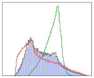
Before constructing the HC-MFM, it is important to look at the LF data. In figure 10, the PDF of the QoI due to the variation of $\alpha$ and $\gamma$ for different training samples of $\kappa$ is represented. The two expected yet important observations are that the PDF of the QoI is significantly influenced by the value of $\kappa$ used in the RANS simulations, and the fact that the PDFs are much different from the ground truth PDF shown in figure 7. The larger influence of $\kappa$ compared with $\alpha$ and $\gamma$ is also reflected in the associated Sobol indices (Sobol Reference Sobol2001), as reported in table 1. Note that the PDF of the QoI considering the simultaneous variation of $\alpha, \gamma$, and $\kappa$ is shown in figure 10(f).

Figure 10.

(a–e) The PDF of $H_{bubble}/h$ at $x/h=2.5$ due to the variation of $\alpha$ and $\gamma$ using the RANS data simulated with $\kappa$ equal to $0.348$, $0.367$, $0.400$, $0.433$, $0.452$, respectively. Note that $5\times 5$ samples are taken from the $\alpha$–$\gamma$ space at each of these constant-$\kappa$ simulations. The PDF in (f) is obtained using all the $5 \times 5 \times 5$ samples from $\alpha, \gamma$ and $\kappa$.

Figure 11.

(a,b) Isolines of the response surface and (c,d) PDF of $H_{bubble}/h$ at $x/h=2.5$ due to the variation of $\alpha$ and $\gamma$ using the HF data of (a,c) case-A and (b,d) case-B. The data are taken from the DNS of Xiao et al. (Reference Xiao, Wi, Laizet and Duan2020) and are specified by dots in (a,b).

The response surface and PDF of the QoI obtained from only the HF data of case-A and case-B are illustrated in figure 11. For case-A with $n_1=4$ HF data, the PDF of the QoI has a plateau which makes it clearly different from the reference PDF in figure 7. By adding only one more DNS data point and obtaining case-B, the response surface becomes more similar to the reference, however, the associated PDF is still single mode. The improved predictions through the application of the HC-MFM are shown in figure 12. Compared with the HF-data in figure 11, the PDFs of the QoI clearly exhibit a second peak for the values between $0.5$ and $0.6$. This peak has been introduced by adding the LF data, see figure 10(f), and this is, in fact, the task for the MFM to adjust the involved hyperparameters such that the fusion of the data at the two fidelities leads to a PDF similar to the reference. Clearly, for case-B with only five DNS data samples included, the PDF and response surface of the QoI are very close to the ground truth in figure 7 (nine DNS). This can also be confirmed by plotting the associated HC-MFM predictions against the reference data at all test points in the $\alpha$–$\gamma$ plane, see figure 13. The joint PDF of these two sets of data for both considered cases is narrow, specifically for case-B, and hence implies a low point-to-point deviation of the predictions from the reference values. It is also interesting to look at the posterior distribution of the RANS calibration parameter $\kappa$. It is not surprising that the resulting PDFs from the multifidelity data sets case-A and case-B are different in spite of having the same uniform prior distribution. Two important observations here are the following: first, in contrast to the previous examples in the present study, even with a small number of HF-data, i.e. case-A, a significantly informative PDF for the LF calibration parameter is obtained. Second, for case-B, the posterior distribution of $\kappa$ is very similar to the reference case where nine DNS data sets are used, see figure 8. Thus, depending on the case, the HC-MFM is capable of calibrating the model parameters in a fairly accurate way at the same time of constructing an accurate predictive model. This somewhat challenges the conclusion which could be drawn from the previous examples in the present study and also by Goh et al. (Reference Goh, Bingham, Holloway, Grosskopf, Kuranz and Rutter2013), where the priority of the HC-MFM is found to make accurate predictions for the QoI rather than providing accurate calibration of the fidelity-specific parameters.

Figure 12.

(a,b) Isolines of the response surface and (c,d) PDF of $H_{bubble}/h$ at $x/h=2.5$ due to the variation of $\alpha$ and $\gamma$ obtained from the HC-MFM with the data of (a,c) case-A and (b,d) case-B. In (c,d), the PDF resulting from the HC-MFM is compared with the PDFs of the ground truth (see figure 7), LF data (LFM, figure 10) and HF data (HFM, figure 11).

Figure 13.

(a,b) Joint and marginal PDFs of $H_{bubble}/h$ at $x/h=2.5$, and (c,d) associated sample posterior distribution of $\kappa$ for (a,c) case-A and (b,d) case-B data sets. In (a,b), the contours belong to the joint PDF with associated values specified in the colour bar.

To conclude the periodic hill example, we can quantify stochastic moments of the QoI as well as the Sobol sensitivity indices (Sobol Reference Sobol2001) due to the uncertainty in $\alpha$ and $\gamma$. These UQ measures are integral quantities over the admissible range of the parameters and can be computed using the reference data (all available DNS), LF, HF and MF data sets. Note that for the LF data, the uncertainty in $\kappa$ is also taken into account. Noting the parameters $\alpha, \gamma$ and $\kappa$ are uniformly distributed and independent from each other, the results summarized in table 1 are obtained using the generalized polynomial chaos expansion (Xiu & Karniadakis Reference Xiu and Karniadakis2002) for the reference and LF data sets, and the Monte Carlo method for the multifidelity cases. All the UQ analyses have been performed using UQit (Rezaeiravesh, Vinuesa & Schlatter Reference Rezaeiravesh, Vinuesa and Schlatter2021). In general, for all cases but the pure LF data, the prediction of the mean and standard deviation of the QoI are close to the reference. For the total Sobol indices, the closest estimates to the reference values is obtained from the HC-MFM applied to case-B, and on the second rank, case-A. Noting the improvement of the Sobol indices accuracy in each of the multifidelity cases compared with the estimates from the associated HF data, the effectiveness of the HC-MFM is once again confirmed. This is an important outcome considering the forward UQ problems and global sensitivity analyses are of most relevance in CFD applications.

3.5. Keeping the RANS parameter fixed

In all the examples in the present study, the fidelity-specific calibration parameters are involved in the multifidelity modelling and posterior distributions for them are learned during the construction of the MFM. But, the methodology behind the HC-MFM described in § 2 is general and flexible to be directly applicable to the cases where the fidelity-specific parameters are kept fixed. To demonstrate this, let us apply the HC-MFM to the example of the periodic hill and use the RANS data at constant values of $\kappa$, the RANS modelling parameter in (3.7). We use the case-B data sets shown in figure 9 which means having $5$ and $25$ samples for the DNS and RANS simulations, respectively, in the $\alpha$–$\gamma$ space. The validation of the PDF of the QoI, $H_{bubble}/h$ at $x/h=2.5$, of the HC-MFM for two values of $\kappa$ is represented in figure 14. Adopting $\kappa =0.433$ ($\beta _\infty ^*=0.084$) shows a clear improvement in the predictions compared with the standard value $\kappa =0.4$ ($\beta _\infty ^*=0.09$). This observation is consistent with the posterior PDF of $\kappa$ in figure 13, where the mode of the distribution is higher than $0.4$. From this test, not only the validity of the HC-MFM for fixed values of the fidelity-specific parameters is confirmed, but also the fact that such accuracy-controlling parameters should be actively part of the data generation and hence the construction of HC-MFM is emphasized.

Figure 14.

Joint and marginal PDFs of $H_{bubble}/h$ at $x/h=2.5$ for case-B data sets using fixed values of $\kappa$ equal to (a) $0.4$ and (b) $0.433$. Note that the PDF of the QoI due to the variation of $\alpha$ and $\gamma$ corresponding to these $\kappa$ values is plotted in figure 10(c,d), respectively.

Another important point is that the good predictive accuracy in figure 14 is obtained despite the poor correlation between the DNS and RANS data. This is because of accurate construction of the model discrepancy term in (3.8) and also accurate estimation of various hyperparameters. It is also noteworthy that the present example is comparable to what is performed by Voet et al. (Reference Voet, Ahlfeld, Gaymann, Laizet and Montomoli2021) using $7$ DNS and $30$ RANS data sets using different multifidelity modelling approaches while fixing the value of the coefficients in the RANS closure model. However, a direct comparison between the two studies is not possible since, in the study by Voet et al. (Reference Voet, Ahlfeld, Gaymann, Laizet and Montomoli2021), the plots of the MFM predictions vs reference values of the QoI as in figure 14 were not provided.

3.6. Impact of replacing the MCMC by a point-estimator

In all the examples presented in this study, the HC-MFM is constructed using the MCMC method to draw samples from the posterior distribution of the hyperparameters and calibration parameters, i.e. $\boldsymbol {\beta }$ and $\boldsymbol {\theta }$, respectively, in the Bayes formula (2.13). Similarly, to predict the sample distribution of the QoI, direct samples from these posterior distributions are used in the HC-MFM. As an alternative to these sample-based methods within the Bayesian framework, point estimators such as maximum a posteriori probability (MAP) and maximum likelihood estimators (MLE) can be adopted. The point-estimated values are considered to be the representatives of the corresponding distribution. Note that the use of the uniform priors in (2.13) makes the MAP estimations identical to the MLE. Our investigations showed that using point estimators instead of the MCMC method, could deteriorate the accuracy of the HC-MFM predictions, independent from how the LF and HF data are combined.

For instance, according to figure 15, the PDF of the QoIs predicted by the HC-MFM using the MAP estimator is significantly worse than what is given by the MCMC method as shown in figure 13. This is an important message of the present study noting that all previous multifidelity studies in the literature relevant to the fluid flows have been based on using the point estimators, see e.g. Voet et al. (Reference Voet, Ahlfeld, Gaymann, Laizet and Montomoli2021) where the MLE is adopted.

Figure 15.

Joint and marginal PDFs of $H_{bubble}/h$ at $x/h=2.5$ for (a) case-A and (b) case-B data sets. Here, a MAP estimator is used to construct the HC-MFM, in contrast to figure 13 and the rest of the examples in the present study which are obtained using an MCMC method.

The reason for this observation is that, to obtain the best fit for the GP-based models, here the HC-MFM, for a given set of data, the global optimum of the parameters appearing in the model should be found. This, in general, is not an easy task considering the optimization problem can be non-convex with many local optima (Rasmussen & Williams Reference Rasmussen and Williams2005; Gramacy Reference Gramacy2020). Depending on the problem, the point estimators such as MAP and MLE may or may not be successful in finding the global optimum. In contrast, a thorough exploration of the admissible space of the parameters via MCMC samples can rectify the issue. More concrete examples and discussion in this regard can be pursued in an extension of the present study.