


1. Introduction
The hyporheic zone comprises the saturated regions of the sediment bed, where the water in the pore space interacts with the stream flow via a bidirectional exchange of momentum, mass and energy (e.g. Boano et al. Reference Boano, Harvey, Marion, Packman, Revelli, Ridolfi and Wörman2014; Woessner Reference Woessner, Richard Hauer and Lamberti2017). Steep biogeochemical gradients in the hyporheic zone create a unique habitat for a rich community of benthic and interstitial organisms (Brunke & Gonser Reference Brunke and Gonser1997; Krause et al. Reference Krause2017). Among the latter are many micro-organisms, which form biofilms on solid surfaces and rely on a steady supply with specific nutrients and dissolved substances, while they also depend on the removal of the end products of their metabolism (e.g. Battin et al. Reference Battin, Besemer, Bengtsson, Romani and Packmann2016). This microbial activity is decisive for the health of the aquatic ecosystem, it maintains different nutrient cycles and can even mitigate anthropogenic eutrophication of the water body (e.g. Harvey et al. Reference Harvey, Böhlke, Voytek, Scott and Tobias2013). Accordingly, mass transport processes across the sediment--water interface are of interdisciplinary interest (e.g. Krause et al. Reference Krause, Hannah, Fleckenstein, Heppell, Kaeser, Pickup, Pinay, Robertson and Wood2011; Ward Reference Ward2016). Depending on the forcing mechanism, these transport processes can occur on different spatial scales, which can typically range up to tens of metres (Boano et al. Reference Boano, Harvey, Marion, Packman, Revelli, Ridolfi and Wörman2014). In contrast to that, hyporheic transport processes can also occur on the critically smaller length scale of individual sediment grains, where primarily hydrodynamic forces tend to drive the flow (Boano et al. Reference Boano, Harvey, Marion, Packman, Revelli, Ridolfi and Wörman2014). The transport processes on the grain-scale have high impact, as they appear over large areas and act within the region shortly below the sediment--water interface, where the ecologically most critical biota are found (Marion et al. Reference Heidi2014). Therefore, the present study focuses on grain-scale hyporheic scalar transport and aims to advance the mechanistic understanding of the processes involved.
The studies of Richardson & Parr (Reference Richardson and Parr1988), Nagaoka & Ohgaki (Reference Nagaoka and Ohgaki1990) and Lai, Lo & Lin (Reference Lai, Lo and Lin1994) were among the first systematic investigations of mass transfer across the interface between a plane sediment bed and an overlying flow. Laboratory flume experiments were conducted to determine effective diffusivity coefficients, which were used to summarise the effects of turbulent transport, dispersive transport and molecular diffusion in the scope of a gradient-based transport model. Subsequent studies performed meta-analyses and combined different data sets to refine the prediction of an effective diffusivity, whereas different sets of input parameters were used.
O’Connor & Harvey (Reference O’Connor and Harvey2008) concluded that the ratio between the effective diffusivity and the tortuosity-adapted molecular diffusivity can be approximated by the product of the roughness Reynolds number and a permeability Péclet number (with an exponent near unity). The value of this product allows the definition of four partially overlapping ranges, which are associated with transport conditions dominated by molecular diffusion, shear-induced flow, advective pumping or penetrating turbulence, respectively. After a correction of biases in the underlying data, Grant, Stewardson & Marusic (Reference Grant, Stewardson and Marusic2012) applied a procedure based on multiple linear regression to isolate a small set of parameters with a high predictive power for the effective diffusivity. A resulting model uses the porosity, the permeability Reynolds number and a Reynolds number based on the bed depth as dimensionless input parameters, which appear with different exponents. In contrast to O’Connor & Harvey (Reference O’Connor and Harvey2008), the roughness length remains unconsidered, which is explained by a strong correlation with other parameters. Voermans, Ghisalberti & Ivey (Reference Voermans, Ghisalberti and Ivey2018) combined insight from their own measurements (Voermans, Ghisalberti & Ivey Reference Voermans, Ghisalberti and Ivey2017) with data points from various other experimental studies (e.g. Richardson & Parr Reference Richardson and Parr1988; Nagaoka & Ohgaki Reference Nagaoka and Ohgaki1990; Packman, Salehin & Zaramella Reference Packman, Salehin and Zaramella2004; Chandler et al. Reference Chandler, Guymer, Pearson and van Egmond2016). On that basis, they proposed a model for the mass transport across the sediment--water interface, which predicts the ratio of effective diffusivity and molecular diffusivity only in dependency of the permeability Reynolds number and the Schmidt number. With a progressively higher permeability Reynolds number, the model describes a transition from the diffusion-dominated regime to the dispersion-dominated regime and from there to a regime dominated by turbulent scalar transport. From the observed scaling behaviour at the transition from the dispersion-dominated regime to the turbulent regime, Voermans et al. (Reference Voermans, Ghisalberti and Ivey2018) deduced that turbulent motion at the interface disrupts dispersive scalar transport. A hypothetical explanation is found in the reduction of the spatial variations in the passive scalar field due to turbulent mixing. Voermans et al. (Reference Voermans, Ghisalberti and Ivey2018) remarked that the permeability Reynolds number is correlated with the roughness Reynolds number, which also indicates the roughness regime. In agreement with this remark, Chen, Fytanidis & Garcia (Reference Chen, Fytanidis and Garcia2024) concluded that the roughness Reynolds number is the preferred input parameter to determine the interfacial effective diffusivity.
Besides the effort invested in effective diffusivity models, several studies also documented qualitative phenomena associated with hyporheic scalar transport. Packman et al. (Reference Packman, Salehin and Zaramella2004) conducted experiments in a laboratory flume for both flat beds and beds with a dune-shaped surface topography. Injected dye allowed a visualisation of the scalar transport. Also in flat-bed sediments, advective flow paths in the bed-normal direction were observed. Though the concept of advective pumping had been described by Elliott & Brooks (Reference Elliott and Brooks1997) for beds with a macroscopic topography, Packman et al. (Reference Packman, Salehin and Zaramella2004) hypothesised that grain-scale irregularities induce pressure head variations, which are sufficient to cause upwelling or downwelling fluid motion. In deeper regions of the sediment bed, dye was sometimes found to follow preferred flow paths, while a pulsating motion suggested an influence from the turbulent flow above the bed. Shen, Yuan & Phanikumar (Reference Shen, Yuan and Phanikumar2020) emphasised the impact of bed roughness on the exchange processes across the interface, while keeping $Re_K$
constant. In the scope of a grain-resolved direct numerical simulation (DNS), they compared synthesised macroscopically flat beds with randomly and regularly arranged spheres at the interface against each other. The random arrangement of spheres at the interface was shown to introduce larger roughness length scales, which cause larger-scale pressure fluctuations at the interface. The resulting flow paths reach deeper into the sediment layer and increase the contribution of dispersive fluxes to the transport of mass and momentum. Thus, the irregular texture of the sediment bed surface also influences the time that an average fluid parcel resides within the sediment bed, as documented by Shen, Yuan & Phanikumar (Reference Shen, Yuan and Phanikumar2022).
$Re_K$
constant. In the scope of a grain-resolved direct numerical simulation (DNS), they compared synthesised macroscopically flat beds with randomly and regularly arranged spheres at the interface against each other. The random arrangement of spheres at the interface was shown to introduce larger roughness length scales, which cause larger-scale pressure fluctuations at the interface. The resulting flow paths reach deeper into the sediment layer and increase the contribution of dispersive fluxes to the transport of mass and momentum. Thus, the irregular texture of the sediment bed surface also influences the time that an average fluid parcel resides within the sediment bed, as documented by Shen, Yuan & Phanikumar (Reference Shen, Yuan and Phanikumar2022).
The above overview emphasises the strong scientific interest in hyporheic scalar transport. Many studies focus on the effective scalar diffusivity and the dominant processes at the interface, whereas different models for the prediction of the interfacial effective diffusivity utilise different input parameters. In recent years, pore-resolved numerical studies have granted valuable insight into the complex and strongly three-dimensional flow field inside the sediment bed, which allowed further conclusions concerning hyporheic scalar transport processes. To our knowledge, however, no pore-resolved single-domain simulations with a wider parameter space have been conducted, which actually solve the advection--diffusion equation for a passive scalar in the context of turbulent flow over a random sphere pack. Building on v.Wenczowski & Manhart (Reference v.Wenczowski and Manhart2024), the present study closes this gap, whereas particular focus is put on the following research questions. (i) Which parameters affect the near-interface scalar transport? (ii) Which scalar transport mechanisms are dominant in different regions? (iii) How do these transport mechanisms interact with each other?
Section 2 contains the underlying equations as well as their formulation within the double-averaging analysis framework. The applied methods and the parameter space with a systematic variation of $Re_\tau$
and
$Re_\tau$
and $Re_K$
are introduced in § 3. In § 4, we present the main results, which are then discussed in § 5. Section 6 concludes the study.
$Re_K$
are introduced in § 3. In § 4, we present the main results, which are then discussed in § 5. Section 6 concludes the study.
2. Theory
The following § 2.1 contains the underlying equations. The double-averaging analysis framework is introduced in § 2.2, which allows us to discuss the double-averaged scalar transport equation in § 2.3. In § 2.4, budget equations for temporal scalar fluctuations and spatial scalar variations are formulated, which will help us later to investigate the interaction between processes.
2.1. Governing equations
Using DNS, we solve the incompressible Navier–Stokes equations for a Newtonian fluid with a kinematic viscosity $\nu$
and a density
$\nu$
and a density $\rho$
. The Einstein summation notation allows us to formulate the conservation of momentum and mass as given by (2.1) and (2.2):
$\rho$
. The Einstein summation notation allows us to formulate the conservation of momentum and mass as given by (2.1) and (2.2):
 \begin{equation} \frac {\partial u_i}{\partial x_i} = 0, \end{equation}
 \begin{equation} \frac {\partial u_i}{\partial t} + u_j \, \frac {\partial u_i}{\partial x_j} = - \frac {1}{\rho } \frac {\partial p}{\partial x_i} + \nu \frac { \partial ^2 u_i }{ \partial x_j \partial x_j } + g_i. \end{equation}
The coordinate $x_1 \equiv x$
represents the streamwise direction,
$x_1 \equiv x$
represents the streamwise direction, $x_2 \equiv y$
represents the spanwise direction and the coordinate
$x_2 \equiv y$
represents the spanwise direction and the coordinate $x_3 \equiv z$
specifies a vertical position above the sediment bed. The corresponding flow velocities are
$x_3 \equiv z$
specifies a vertical position above the sediment bed. The corresponding flow velocities are $u_1 \equiv u$
,
$u_1 \equiv u$
, $u_2 \equiv v$
and
$u_2 \equiv v$
and $u_3 \equiv w$
, respectively. Furthermore,
$u_3 \equiv w$
, respectively. Furthermore, $p$
represents the pressure and
$p$
represents the pressure and $g_i$
is a volume force acting on the fluid. The computed flow field is used in the solution of the advection--diffusion equation for a passive scalar, which reads
$g_i$
is a volume force acting on the fluid. The computed flow field is used in the solution of the advection--diffusion equation for a passive scalar, which reads
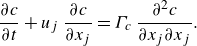 \begin{equation} \frac {\partial c}{\partial t} + u_j \: \frac {\partial c}{\partial x_j} = \Gamma _c \: \frac {\partial ^2 c}{\partial x_j \partial x_j}. \end{equation}
In (2.3) the variable $c$
represents the scalar concentration and
$c$
represents the scalar concentration and $\Gamma _c$
is the corresponding scalar diffusion coefficient. As we consider a Schmidt number of
$\Gamma _c$
is the corresponding scalar diffusion coefficient. As we consider a Schmidt number of $Sc = \nu / \Gamma _c = 1$
, the Batchelor length scale is similar to the Kolmogorov length scale. Under steady conditions, the dimensionless form of (2.3) reduces to
$Sc = \nu / \Gamma _c = 1$
, the Batchelor length scale is similar to the Kolmogorov length scale. Under steady conditions, the dimensionless form of (2.3) reduces to
 \begin{equation} \hat {u}_j \: \frac {\partial \hat {c}}{\partial \hat {x}_j} = \frac {1}{\textit{Pe}} \, \frac {\partial ^2 \hat {c}}{\partial \hat {x}_j \partial \hat {x}_j} . \end{equation}
In (2.4), $\textit{Pe} = Re \, Sc$
represents the dimensionless Péclet number, which describes the ratio between the diffusive and the advective term. If one wished to interpret the passive scalar
$\textit{Pe} = Re \, Sc$
represents the dimensionless Péclet number, which describes the ratio between the diffusive and the advective term. If one wished to interpret the passive scalar $c$
as a temperature (without buoyancy effects),
$c$
as a temperature (without buoyancy effects), $\Gamma _c$
would correspond to the thermal diffusivity and the Schmidt number
$\Gamma _c$
would correspond to the thermal diffusivity and the Schmidt number $Sc$
would be replaced by the Prandtl number
$Sc$
would be replaced by the Prandtl number $Pr$
.
$Pr$
.
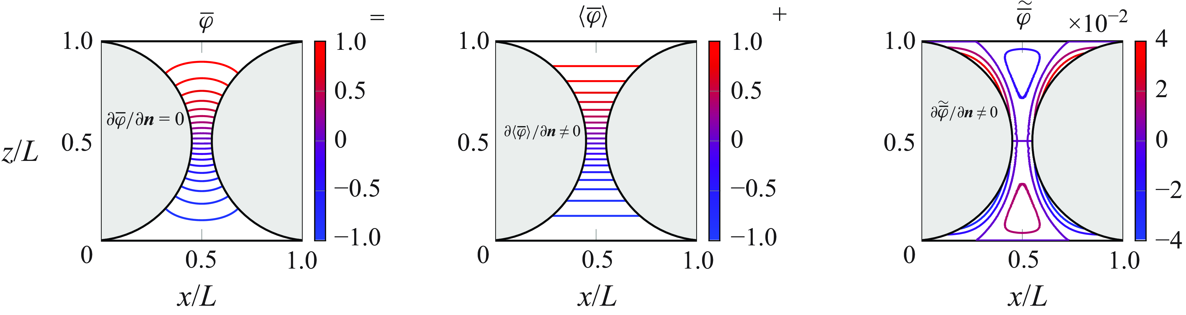
Diffusion problem with decomposition of the solution into intrinsic horizontal averages and spatial variations. In contrast to the actual solution, both the intrinsic averages and the spatial variations violate the zero-flux (adiabatic) Neumann boundary conditions.
2.2. Analysis framework
Double averaging in time and space provides a useful analysis framework for hyporheic scalar transport (e.g. Giménez-Curto & Lera Reference Giménez-Curto and Lera1996; Nikora et al. Reference Nikora, Goring, McEwan and Griffiths2001; Mignot, Barthelemy & Hurther Reference Mignot, Barthelemy and Hurther2009). In a first step, the arbitrary quantity $\varphi$
undergoes a Reynolds decomposition. The ensemble average in time is denoted as
$\varphi$
undergoes a Reynolds decomposition. The ensemble average in time is denoted as $\overline {\varphi }$
, while
$\overline {\varphi }$
, while $\varphi '$
represents a temporal fluctuation of the quantity, such that
$\varphi '$
represents a temporal fluctuation of the quantity, such that
 \begin{equation} \varphi {( \boldsymbol{x},t)} = \overline {\varphi }{(\boldsymbol{x})} + \varphi ^\prime {(\boldsymbol{x},t)} \;, \qquad \text{where} \qquad \overline {\varphi }{(\boldsymbol{x})} = \frac {1}{T} \int _{0}^{T} \varphi {(\boldsymbol{x},t)} \: {\rm d}t .\end{equation}
In the following, $\overline {\varphi }$
is further decomposed with respect to its spatial distribution. The intrinsic average within a horizontal plane is written as
$\overline {\varphi }$
is further decomposed with respect to its spatial distribution. The intrinsic average within a horizontal plane is written as $\left \langle \overline {\varphi } \right \rangle$
. Deviations from the in-plane average represent spatial variations and are marked by a tilde, such that
$\left \langle \overline {\varphi } \right \rangle$
. Deviations from the in-plane average represent spatial variations and are marked by a tilde, such that
 \begin{equation} \overline {\varphi }{(\boldsymbol{x})} = \langle \overline {\varphi } \rangle {(z)} + \widetilde {\overline {\varphi }}{(\boldsymbol{x})} \;, \qquad \text{where} \qquad \langle \overline {\varphi } \rangle {(z)} = \frac {1}{A_{f}} \iint _{A_f} \overline {\varphi }{(\boldsymbol{x})} \: {\rm d}x \: {\rm d}y. \end{equation}
The intrinsic average $\left \langle \overline { \varphi } \right \rangle$
is defined by (2.6) and results from averaging over the fluid-filled area
$\left \langle \overline { \varphi } \right \rangle$
is defined by (2.6) and results from averaging over the fluid-filled area $A_f$
of the averaging plane at height
$A_f$
of the averaging plane at height $z$
. In contrast, the superficial average
$z$
. In contrast, the superficial average $\left \langle \overline { \varphi } \right \rangle ^s$
represents a spatial mean value with respect to the complete area
$\left \langle \overline { \varphi } \right \rangle ^s$
represents a spatial mean value with respect to the complete area $A_0$
of the averaging plane, such that both quantities are connected via the in-plane porosity
$A_0$
of the averaging plane, such that both quantities are connected via the in-plane porosity $\theta {(z)}$
, i.e.
$\theta {(z)}$
, i.e.
 \begin{equation} \left \langle \overline {\varphi } \right \rangle ^s{(z)} = \theta {(z)} \: \left \langle \overline {\varphi } \right \rangle {(z)}, \quad \text{with} \quad \theta {(z)} = {A_{f}(z)} / {A_0}. \end{equation}
Below the crests of the topmost spheres of the sphere pack, the fluid-filled area $A_f$
in the averaging plane is interrupted by solid-occupied areas. In general, however, the physical boundary conditions on the fluid--solid interface are neither fulfilled by
$A_f$
in the averaging plane is interrupted by solid-occupied areas. In general, however, the physical boundary conditions on the fluid--solid interface are neither fulfilled by $ \langle \overline {\varphi } \rangle$
nor by
$ \langle \overline {\varphi } \rangle$
nor by $ \widetilde {\overline {\varphi }}$
, individually. As a consequence, horizontal averaging and spatial derivatives do not simply commute and special rules apply (e.g. Giménez-Curto & Lera Reference Giménez-Curto and Lera1996), which gives
$ \widetilde {\overline {\varphi }}$
, individually. As a consequence, horizontal averaging and spatial derivatives do not simply commute and special rules apply (e.g. Giménez-Curto & Lera Reference Giménez-Curto and Lera1996), which gives
 \begin{eqnarray} \displaystyle \left \langle \nabla \overline {\varphi } \right \rangle = \left (\def\negativespace{} \begin{matrix} \displaystyle \left \langle \frac {\partial \overline {\varphi }}{\partial x} \right \rangle \\[3ex] \displaystyle \left \langle \frac {\partial \overline {\varphi }}{\partial y} \right \rangle \\[3ex] \displaystyle \left \langle \frac {\partial \overline {\varphi }}{\partial z} \right \rangle \end{matrix} \def\negativespace{} \right ) = \left (\def\negativespace{} \begin{matrix} \displaystyle \frac {1}{A_f} \oint _s \: \overline {\varphi } \: \frac {n_x}{\sqrt {n_x^2 + n_y^2}} \: {\rm d}s \\[3ex] \displaystyle \frac {1}{A_f} \oint _s \: \overline {\varphi } \: \frac {n_y}{\sqrt {n_x^2 + n_y^2}} \:{\rm d}s \\[4ex] \displaystyle \frac {1}{\theta } \frac {\partial \theta \left \langle \overline {\varphi } \right \rangle }{\partial z} + \frac {1}{A_f} \oint _s \:\overline {\varphi } \: \frac {n_z}{\sqrt {n_x^2 + n_y^2}} \:{\rm d}s \end{matrix}\def\negativespace{} \right ) \triangleq \left ( \begin{matrix} \displaystyle \text{BT}_1( \overline {\varphi } ) \\[4ex] \displaystyle \text{BT}_2( \overline {\varphi } ) \\[3ex] \displaystyle \frac {1}{\theta } \frac {\partial \theta \left \langle \overline {\varphi } \right \rangle }{\partial z} +\text{BT}_3( \overline {\varphi } ) \end{matrix} \def\negativespace{}\right )\def\negativespace{}. \nonumber\\[-12pt]\end{eqnarray}
In (2.8) the curve $s$
represents the intersection of the averaging plane with the fluid--solid interface. The unit normal vector
$s$
represents the intersection of the averaging plane with the fluid--solid interface. The unit normal vector $\boldsymbol{n} = (n_x, n_y, n_z)^T$
at the solid--fluid interface points out of the fluid-filled volume. We will refer to the curve integrals as boundary terms, abbreviated by
$\boldsymbol{n} = (n_x, n_y, n_z)^T$
at the solid--fluid interface points out of the fluid-filled volume. We will refer to the curve integrals as boundary terms, abbreviated by $\text{BT}_i(\overline {\varphi })$
. By that, we emphasise that the terms are necessary to take into account for the physical boundary conditions, which are met by
$\text{BT}_i(\overline {\varphi })$
. By that, we emphasise that the terms are necessary to take into account for the physical boundary conditions, which are met by $\overline {\varphi }$
and
$\overline {\varphi }$
and $\varphi ^\prime$
, but not by
$\varphi ^\prime$
, but not by $\langle \overline {\varphi } \rangle$
and
$\langle \overline {\varphi } \rangle$
and $\widetilde {\overline {\varphi }}$
. This issue is illustrated by figure 1 for the solution of a two-dimensional diffusion problem with adiabatic boundary conditions on curved boundaries, which enforce that
$\widetilde {\overline {\varphi }}$
. This issue is illustrated by figure 1 for the solution of a two-dimensional diffusion problem with adiabatic boundary conditions on curved boundaries, which enforce that $\partial \overline {\varphi } / \partial \boldsymbol{n} = 0$
. While the field
$\partial \overline {\varphi } / \partial \boldsymbol{n} = 0$
. While the field $\overline {\varphi }$
fulfills this condition, both
$\overline {\varphi }$
fulfills this condition, both $\langle \overline {\varphi } \rangle$
and
$\langle \overline {\varphi } \rangle$
and $\widetilde {\overline {\varphi }}$
have non-zero wall-normal gradients, which would cause unphysical wall-normal diffusive fluxes of these quantities. These unphysical fluxes have opposite signs and compensate each other.
$\widetilde {\overline {\varphi }}$
have non-zero wall-normal gradients, which would cause unphysical wall-normal diffusive fluxes of these quantities. These unphysical fluxes have opposite signs and compensate each other.
2.3. Scalar transport processes
In view of the application, we derive the equations under the assumption that no-slip conditions apply on the surface of the sediment grains. Furthermore, we assume that no net flux in the bed-normal direction exists, i.e. $\left \langle \overline {w} \right \rangle = 0$
. The surface of the sediment grains is defined to be impermeable to (diffusive) scalar fluxes, which resembles adiabatic conditions. Therefore, the superficially averaged scalar flux
$\left \langle \overline {w} \right \rangle = 0$
. The surface of the sediment grains is defined to be impermeable to (diffusive) scalar fluxes, which resembles adiabatic conditions. Therefore, the superficially averaged scalar flux $\langle \overline {J} \rangle ^s_{\textit{tot}}$
across all horizontal planes must be constant, while contributions from different scalar transport processes can be distinguished:
$\langle \overline {J} \rangle ^s_{\textit{tot}}$
across all horizontal planes must be constant, while contributions from different scalar transport processes can be distinguished:
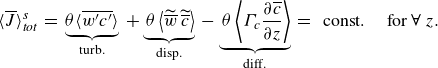 \begin{equation} \langle \overline {J} \rangle ^s_{\textit{tot}} \, = \; \underbrace { \theta \langle \overline {w^\prime c^\prime } \rangle }_{\text{turb.}} \; + \underbrace { \; \theta \left \langle \widetilde {\overline {w}} \: \widetilde {\overline {c}} \right \rangle }_{\text{disp.}} \; - \underbrace { \; \theta \left \langle \Gamma _c \frac {\partial \overline {c}}{\partial z} \right \rangle }_{\text{diff.}} \; = \; \text{ const. } \quad \text{for}\ \forall \ z .\end{equation}
The terms on the right-hand side of (2.9) represent fluxes from turbulent scalar transport, dispersive scalar transport and scalar transport due to molecular diffusion. These transport processes rely on fundamentally different mechanisms: Turbulent transport results from temporally correlated fluctuations of the bed-normal velocity and the scalar concentration. In contrast, the dispersive transport depends on spatially correlated in-plane variations of the mean velocity and the mean scalar concentration. Finally, the diffusive flux term is induced by gradients of the concentration field in the bed-normal direction.
2.4. Budget equations
As both temporal fluctuations and spatial variations of the scalar concentration field play an important role for scalar transport (see (2.9)), we consider the budget equations for both quantities:
 @@
@@
 @@
@@
A comparison of (2.10) and (2.11) shows similar patterns in the formulation of both budgets, which contain a production term, a dissipation term, as well as terms for advective, turbulent and diffusive transport. The production part of the budgets is further subdivided: the term in the dashed box leads to a positive production of $\langle \overline {c'c'} \rangle$
or
$\langle \overline {c'c'} \rangle$
or $\langle \widetilde {\overline {c}} \, \widetilde {\overline {c}} \rangle$
, if turbulent or dispersive scalar transport, respectively, acts against the gradient of the double-averaged scalar concentration field. Accordingly, we will refer to these terms as turbulent or dispersive gradient production, respectively. The terms in the solid boxes appear with opposite signs in the budget equations and, therefore, represents a transfer mechanism between temporal fluctuations and spatial variations. Temporal scalar fluctuations
$\langle \widetilde {\overline {c}} \, \widetilde {\overline {c}} \rangle$
, if turbulent or dispersive scalar transport, respectively, acts against the gradient of the double-averaged scalar concentration field. Accordingly, we will refer to these terms as turbulent or dispersive gradient production, respectively. The terms in the solid boxes appear with opposite signs in the budget equations and, therefore, represents a transfer mechanism between temporal fluctuations and spatial variations. Temporal scalar fluctuations $\langle \overline {c'c'} \rangle$
are generated at the expense of spatial scalar variations
$\langle \overline {c'c'} \rangle$
are generated at the expense of spatial scalar variations $\langle \widetilde {\overline {c}} \, \widetilde {\overline {c}} \rangle$
, if turbulent scalar transport takes place against the gradient of the scalar variation, thus homogenizing the in-plane scalar field. In smooth-wall channel flow,
$\langle \widetilde {\overline {c}} \, \widetilde {\overline {c}} \rangle$
, if turbulent scalar transport takes place against the gradient of the scalar variation, thus homogenizing the in-plane scalar field. In smooth-wall channel flow, $\widetilde {\overline {c}}$
has zero value, such that only the presence of a characteristic geometry renders the production mechanism relevant. Therefore, the mechanism is referred to as form-induced production of temporal scalar fluctuations. Besides the already discussed terms, (2.11) contains a boundary term. This term arises as both
$\widetilde {\overline {c}}$
has zero value, such that only the presence of a characteristic geometry renders the production mechanism relevant. Therefore, the mechanism is referred to as form-induced production of temporal scalar fluctuations. Besides the already discussed terms, (2.11) contains a boundary term. This term arises as both $\langle \overline {c} \rangle$
and
$\langle \overline {c} \rangle$
and $\widetilde {\overline {c}}$
violate the boundary condition by inducing non-zero diffusive fluxes of opposite signs across the zero-flux boundary. Formally, the boundary term represents a redistribution of
$\widetilde {\overline {c}}$
violate the boundary condition by inducing non-zero diffusive fluxes of opposite signs across the zero-flux boundary. Formally, the boundary term represents a redistribution of $\, \overline {c} \, \overline {c} \,$
between
$\, \overline {c} \, \overline {c} \,$
between $\langle \overline {c} \rangle \langle \overline {c} \rangle$
and
$\langle \overline {c} \rangle \langle \overline {c} \rangle$
and $\langle \widetilde {\overline {c}} \, \widetilde {\overline {c}} \rangle$
by means of these fluxes across the boundary. The role of the boundary term is highlighted by the diffusion problem in figure 1, in which the Neumann boundary condition on the inclined walls acts as the only source of spatial variations under zero-velocity conditions.
$\langle \widetilde {\overline {c}} \, \widetilde {\overline {c}} \rangle$
by means of these fluxes across the boundary. The role of the boundary term is highlighted by the diffusion problem in figure 1, in which the Neumann boundary condition on the inclined walls acts as the only source of spatial variations under zero-velocity conditions.
3. Methods
The case configuration is described in § 3.1 and the representation of the porous medium in § 3.2. The parameter space is introduced in § 3.3, before we discuss the interface definition in § 3.4. Section 3.5 focuses on the numerical methods, and a convergence study follows in § 3.6. Some aspects of this section are described in greater detail in v.Wenczowski & Manhart (Reference v.Wenczowski and Manhart2024), where we validated the flow field.
3.1. Case configuration
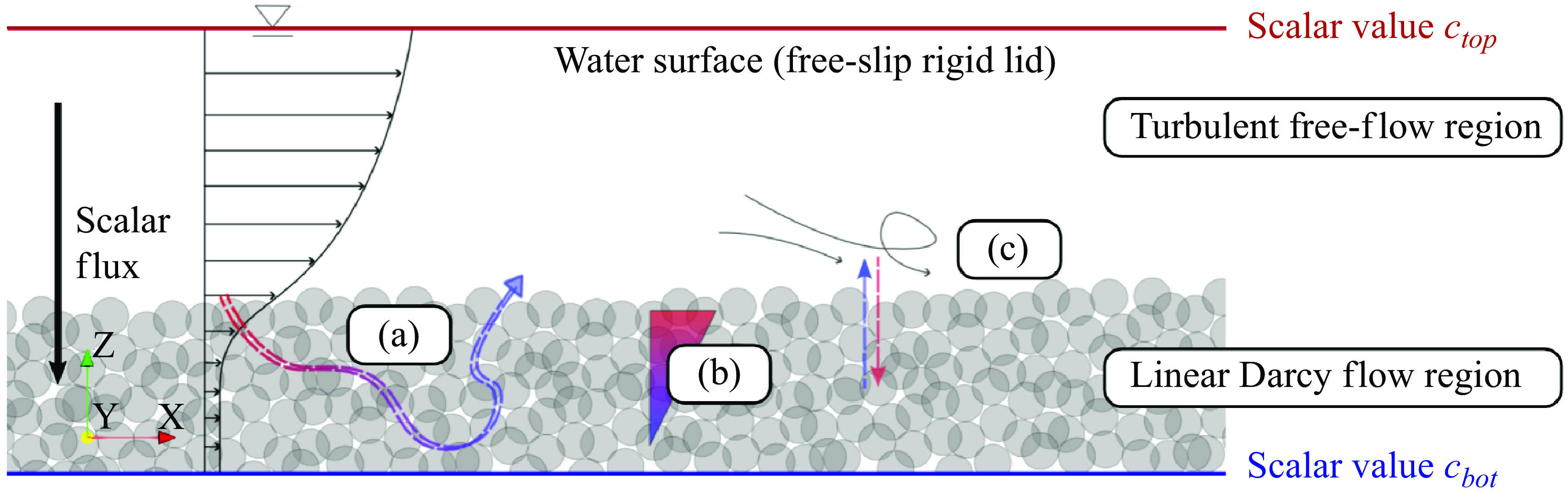
In the scope of a single-domain DNS, we investigate turbulent open-channel flow over a mono-disperse random sphere pack. This configuration resembles the flow in a gravel-bed river, as the sphere pack imitates the sediment bed and individual spheres act as sediment grains. As sketched in figure 2, the top boundary of the domain is a rigid lid with a free-slip boundary condition, which approximates the free water surface. A constant volume force in the streamwise direction, i.e. $g_x \gt 0$
, acts on the fluid and drives the flow. The domain has periodic domain boundary conditions in the streamwise
$g_x \gt 0$
, acts on the fluid and drives the flow. The domain has periodic domain boundary conditions in the streamwise $x$
-direction and lateral
$x$
-direction and lateral $y$
-direction. The simulation statistics are gathered in a statistically stationary state, where the boundary layer is fully developed and the boundary layer thickness
$y$
-direction. The simulation statistics are gathered in a statistically stationary state, where the boundary layer is fully developed and the boundary layer thickness $\delta$
equals the flow depth
$\delta$
equals the flow depth $h$
. During the flow simulation, the spheres with diameter
$h$
. During the flow simulation, the spheres with diameter $D$
remain in fixed positions and no-slip boundary conditions apply on the sphere surfaces. The bottom boundary of the domain cuts through the sphere pack. A free-slip condition reduces the influence of the bottom domain boundary, as it ensures that streamwise momentum is only absorbed by the spheres and not by the domain boundary. Dirichlet boundary conditions prescribe fixed scalar concentration values
$D$
remain in fixed positions and no-slip boundary conditions apply on the sphere surfaces. The bottom boundary of the domain cuts through the sphere pack. A free-slip condition reduces the influence of the bottom domain boundary, as it ensures that streamwise momentum is only absorbed by the spheres and not by the domain boundary. Dirichlet boundary conditions prescribe fixed scalar concentration values $c_{\textit{bot}}$
and
$c_{\textit{bot}}$
and $c_{\textit{top}}$
at the bottom and top domain boundary, respectively. The concentration difference
$c_{\textit{top}}$
at the bottom and top domain boundary, respectively. The concentration difference $\Delta c = c_{\textit{top}} - c_{\textit{bot}}$
induces a scalar flux in the bed-normal direction. The surfaces of the spheres are impermeable to scalar fluxes, which is equivalent to adiabatic conditions in heat transport. In the absence of any scalar sinks or sources, the superficially double-averaged scalar flux is constant at all vertical positions
$\Delta c = c_{\textit{top}} - c_{\textit{bot}}$
induces a scalar flux in the bed-normal direction. The surfaces of the spheres are impermeable to scalar fluxes, which is equivalent to adiabatic conditions in heat transport. In the absence of any scalar sinks or sources, the superficially double-averaged scalar flux is constant at all vertical positions $z$
within the domain (see (2.9)).
$z$
within the domain (see (2.9)).
Sketch of case configuration. The bed-normal scalar flux is induced by fixed scalar values at the bottom and top of the domain. Dispersive transport due to mean flow paths through the sediment (a), diffusive transport due to scalar concentration gradients (b) and turbulent transport due to turbulent fluid motion (c) contribute to the scalar flux.
3.2. Representation of the porous medium
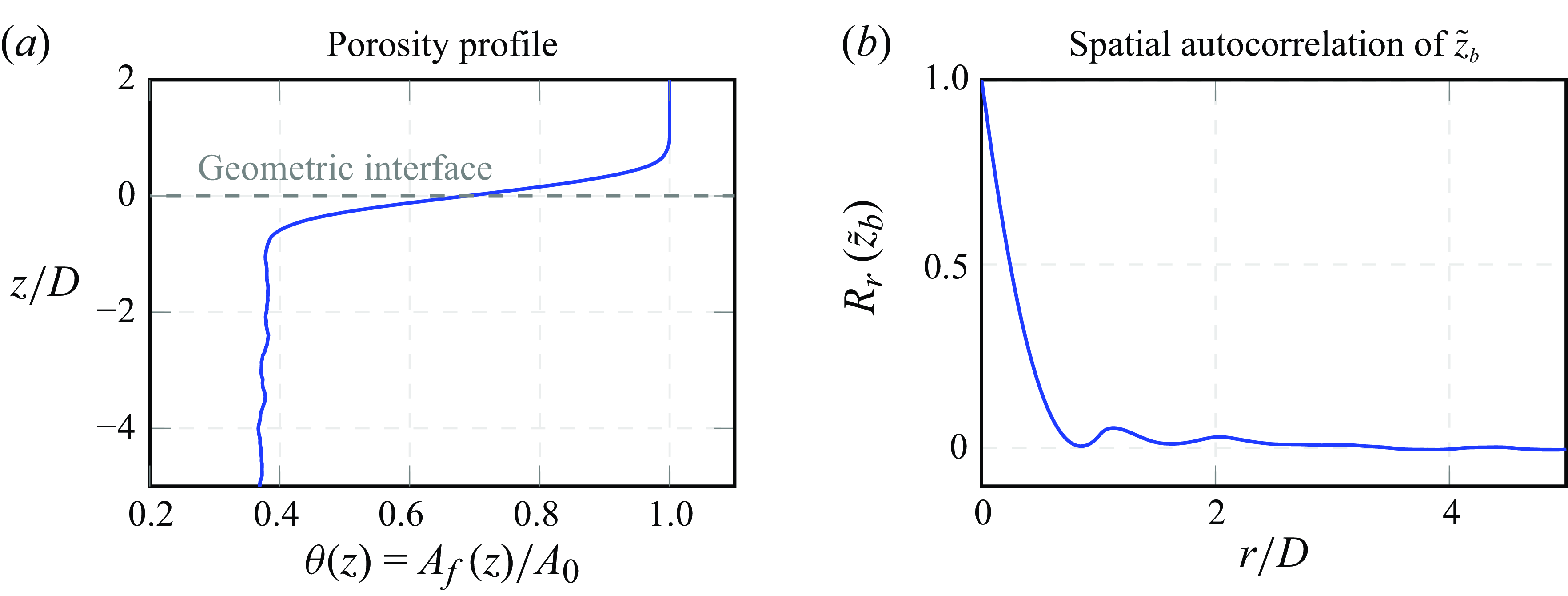
In preparation for the flow simulations, mono-disperse random sphere packs of different extents were generated, as described in v.Wenczowski & Manhart (Reference v.Wenczowski and Manhart2024). The generated sphere packs have a level mean bed surface, as we do not consider bed forms like, e.g. riffles or dunes. The in-plane porosity profile $\theta (z)$
of a sphere pack with a base area of
$\theta (z)$
of a sphere pack with a base area of $A_0 = 64D \times 32D$
is shown in figure 3(a). Like Voermans et al. (Reference Voermans, Ghisalberti and Ivey2017), we use the inflection point
$A_0 = 64D \times 32D$
is shown in figure 3(a). Like Voermans et al. (Reference Voermans, Ghisalberti and Ivey2017), we use the inflection point $\partial ^2 \theta / \partial z^2 = 0$
of the porosity profile as a geometrically defined interface position. The distance between the geometrically determined interface and the top boundary of the domain defines the nominal flow depth
$\partial ^2 \theta / \partial z^2 = 0$
of the porosity profile as a geometrically defined interface position. The distance between the geometrically determined interface and the top boundary of the domain defines the nominal flow depth $h$
of the case. For all simulated cases, the sediment bed has a depth of
$h$
of the case. For all simulated cases, the sediment bed has a depth of $5 \, D$
. At each location, the bed elevation
$5 \, D$
. At each location, the bed elevation $z_b(x,y)$
is defined as the topmost point, where a vertical line at this location would intersect a sphere surface. The derived variable
$z_b(x,y)$
is defined as the topmost point, where a vertical line at this location would intersect a sphere surface. The derived variable $\tilde {z}_b$
represents the spatial variation of the bed elevation field around its mean value. Figure 3(b) shows the spatial autocorrelation of the bed elevation
$\tilde {z}_b$
represents the spatial variation of the bed elevation field around its mean value. Figure 3(b) shows the spatial autocorrelation of the bed elevation $\tilde {z}_b$
. A rapid decay of the spatial autocorrelation function over the distance
$\tilde {z}_b$
. A rapid decay of the spatial autocorrelation function over the distance $r$
confirms that no repeating large-scale patterns prevail in the bed surface.
$r$
confirms that no repeating large-scale patterns prevail in the bed surface.
Properties of a sediment bed with $A_0 = 64D \times 32D$
. (a) In-plane porosity profile with the geometric interface
$A_0 = 64D \times 32D$
. (a) In-plane porosity profile with the geometric interface $z=0$
defined by
$z=0$
defined by $\partial ^2 \theta / \partial z^2 = 0$
. (b) Spatial autocorrelation of the bed elevation fluctuation
$\partial ^2 \theta / \partial z^2 = 0$
. (b) Spatial autocorrelation of the bed elevation fluctuation $\tilde {z}_b$
over the horizontal shift
$\tilde {z}_b$
over the horizontal shift $r$
.
$r$
.
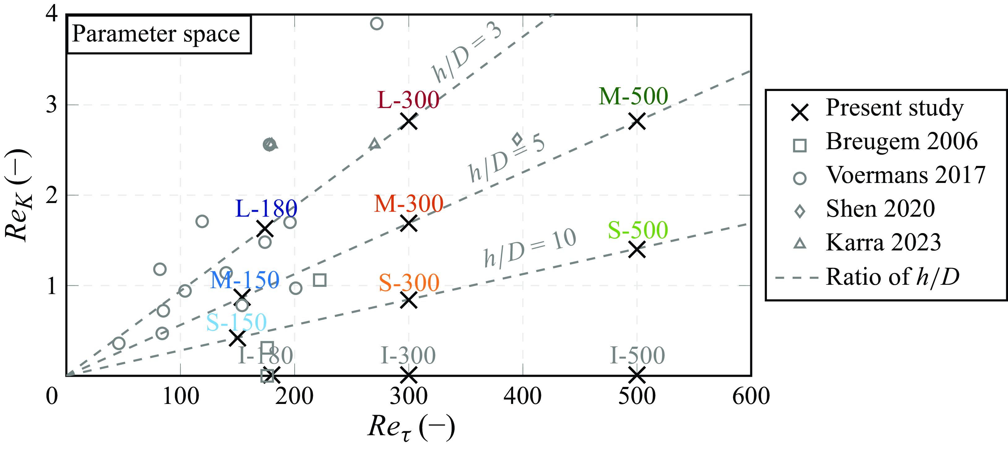
3.3. Parameter space
The parameter space of the present study is described in terms of the friction Reynolds number $Re_\tau$
and permeability Reynolds number
$Re_\tau$
and permeability Reynolds number $Re_K$
. The friction Reynolds number
$Re_K$
. The friction Reynolds number $Re_\tau = u_\tau h / \nu$
characterises the unconfined flow above the sediment layer, where similarities to smooth-wall open-channel flow prevail. The available computing power limited the Reynolds number to
$Re_\tau = u_\tau h / \nu$
characterises the unconfined flow above the sediment layer, where similarities to smooth-wall open-channel flow prevail. The available computing power limited the Reynolds number to $Re_\tau \lt 500$
. The permeability Reynolds number
$Re_\tau \lt 500$
. The permeability Reynolds number $Re_K = u_\tau \sqrt {K} / \nu$
uses the square root of the permeability as an effective length scale of the pore space (Breugem, Boersma & Uittenbogaard Reference Breugem, Boersma and Uittenbogaard2006). By putting
$Re_K = u_\tau \sqrt {K} / \nu$
uses the square root of the permeability as an effective length scale of the pore space (Breugem, Boersma & Uittenbogaard Reference Breugem, Boersma and Uittenbogaard2006). By putting $\sqrt {K}$
in relation to the viscous length scale
$\sqrt {K}$
in relation to the viscous length scale $\delta _\tau = \nu / u_\tau$
,
$\delta _\tau = \nu / u_\tau$
, $Re_K$
gives an indication whether the smallest-scale turbulent motion can penetrate the pore space or not. Therefore,
$Re_K$
gives an indication whether the smallest-scale turbulent motion can penetrate the pore space or not. Therefore, $Re_K \ll 1$
and
$Re_K \ll 1$
and $Re_K \gg 1$
represent effectively impermeable and highly permeable regimes, respectively. Values of
$Re_K \gg 1$
represent effectively impermeable and highly permeable regimes, respectively. Values of $Re_K \approx 1 - 2$
mark the transition between both extremes (Voermans et al. Reference Voermans, Ghisalberti and Ivey2017). The cases are characterised by different ratios of the flow depth to the sphere diameter, i.e.
$Re_K \approx 1 - 2$
mark the transition between both extremes (Voermans et al. Reference Voermans, Ghisalberti and Ivey2017). The cases are characterised by different ratios of the flow depth to the sphere diameter, i.e. $h/D$
, which allows different combinations of
$h/D$
, which allows different combinations of $Re_\tau$
and
$Re_\tau$
and $Re_K$
, as shown in figure 4. Besides the Reynolds numbers, table 1 summarises further nominal parameters of the simulated flow cases. We use the term nominal parameters to indicate that those parameters refer to the a priori geometrically defined flow depth
$Re_K$
, as shown in figure 4. Besides the Reynolds numbers, table 1 summarises further nominal parameters of the simulated flow cases. We use the term nominal parameters to indicate that those parameters refer to the a priori geometrically defined flow depth $h$
and the friction velocity
$h$
and the friction velocity $u_\tau = \sqrt {g_x h}$
.
$u_\tau = \sqrt {g_x h}$
.
Simulated cases as sampling points within a dimensionless parameter space, including reference points from literature. The grey dashed lines represent fixed ratios between the flow depth $h$
and the sphere diameter
$h$
and the sphere diameter $D$
. The reference points refer to Breugem et al. (Reference Breugem, Boersma and Uittenbogaard2006), Voermans et al. (Reference Voermans, Ghisalberti and Ivey2017), Shen et al. (Reference Shen, Yuan and Phanikumar2020) and Karra et al. (Reference Karra, Apte, He and Scheibe2023). Figure adapted from v.Wenczowski & Manhart (Reference v.Wenczowski and Manhart2024).
$D$
. The reference points refer to Breugem et al. (Reference Breugem, Boersma and Uittenbogaard2006), Voermans et al. (Reference Voermans, Ghisalberti and Ivey2017), Shen et al. (Reference Shen, Yuan and Phanikumar2020) and Karra et al. (Reference Karra, Apte, He and Scheibe2023). Figure adapted from v.Wenczowski & Manhart (Reference v.Wenczowski and Manhart2024).
While the transport of gases in air is described by $Sc = O(1)$
, the transport of dissolved substances in water is usually characterised by critically higher Schmidt numbers of
$Sc = O(1)$
, the transport of dissolved substances in water is usually characterised by critically higher Schmidt numbers of $Sc = O(10^3)$
. Still, we consider a unitary Schmidt number ideal for the present study, as it will allow us to observe both diffusion- and advection-dominated hyporheic regimes within the range of
$Sc = O(10^3)$
. Still, we consider a unitary Schmidt number ideal for the present study, as it will allow us to observe both diffusion- and advection-dominated hyporheic regimes within the range of $Re_K \in [0.4, 2.8]$
. From a practical perspective, the choice of
$Re_K \in [0.4, 2.8]$
. From a practical perspective, the choice of $Sc=1$
allows us to keep control of the required grid resolution, while the comparatively short diffusive time scale reduces the amount of simulated time until a steady state is reached.
$Sc=1$
allows us to keep control of the required grid resolution, while the comparatively short diffusive time scale reduces the amount of simulated time until a steady state is reached.
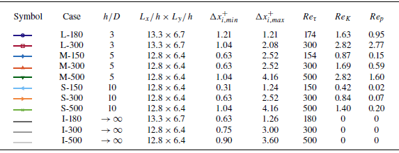
Overview of nominal case parameters. The variable $h$
represents the flow depth above the geometrically defined interface,
$h$
represents the flow depth above the geometrically defined interface, $D$
is the sphere diameter,
$D$
is the sphere diameter, $L$
is the extent of the domain,
$L$
is the extent of the domain, $\Delta x_{i,min}^+$
describes the side length of the smallest cubic cells near the interface and
$\Delta x_{i,min}^+$
describes the side length of the smallest cubic cells near the interface and $\Delta x_{i,max}^+$
the side length of the largest cells in the free-flow region. The friction, permeability and particle Reynolds numbers are defined as
$\Delta x_{i,max}^+$
the side length of the largest cells in the free-flow region. The friction, permeability and particle Reynolds numbers are defined as $Re_\tau = u_\tau h / \nu$
,
$Re_\tau = u_\tau h / \nu$
, $Re_K = u_\tau \sqrt {K} / \nu$
,
$Re_K = u_\tau \sqrt {K} / \nu$
, $Re_p = \langle \overline {u} \rangle ^s D / \nu$
, respectively, where
$Re_p = \langle \overline {u} \rangle ^s D / \nu$
, respectively, where $u_\tau = \sqrt {g_x h}$
is the friction velocity,
$u_\tau = \sqrt {g_x h}$
is the friction velocity, $K$
the permeability and
$K$
the permeability and $\nu$
the kinematic viscosity.
$\nu$
the kinematic viscosity.
3.4. Interface position
The geometrically defined interface is determined from the porosity profile of the sphere pack, such that this interface is available during the configuration phase of the simulations, while it lacks flow-dynamical motivation. To discuss the scalar transport across the interface between a porous medium and a free turbulent flow and to find similarities, a flow-dynamically meaningful interface definition is required, which can be obtained a posteriori from the simulation results. As described in v.Wenczowski & Manhart (Reference v.Wenczowski and Manhart2024) in greater detail, we computed the superficially double-averaged drag distribution $f_{(p+\nu )}^s$
on the porous medium via the relation
$f_{(p+\nu )}^s$
on the porous medium via the relation
 \begin{equation} f_{(p+\nu )}^s = \frac {\partial }{\partial z} \left ( - \theta \left \langle \nu \frac {\partial \, \overline {u}}{\partial z} \right \rangle + \theta \left \langle \widetilde {\overline {u}} \, \widetilde {\overline {w}} \right \rangle + \theta \langle \overline {u^\prime w^\prime } \rangle \right ) - \theta \, g_x . \end{equation}
The expression in (3.1) results from the double-averaged Navier–Stokes equation (e.g. Nikora et al. Reference Nikora, Goring, McEwan and Griffiths2001), while we summarise both viscous and pressure drag in $f_{(p+\nu )}^s$
. The obtained drag distribution exhibits a characteristic peak near the sediment–water interface, which can be associated with the absorption of incoming momentum from the free-flow region. Inspired by the idea of Thom (Reference Thom1971) and Jackson (Reference Jackson1981), we apply a curve fitting approach to characterise the free-flow momentum absorption peak by few parameters and to distinguish it from the Darcy drag, which is exerted by the porous media flow independently of the free flow above. In our fitting function, a Gaussian normal distribution is used to parametrise the free-flow momentum absorption peak, while a complementary error function ensures that the Darcy drag is only accounted for below the interface. Both terms of our fitting function
$f_{(p+\nu )}^s$
. The obtained drag distribution exhibits a characteristic peak near the sediment–water interface, which can be associated with the absorption of incoming momentum from the free-flow region. Inspired by the idea of Thom (Reference Thom1971) and Jackson (Reference Jackson1981), we apply a curve fitting approach to characterise the free-flow momentum absorption peak by few parameters and to distinguish it from the Darcy drag, which is exerted by the porous media flow independently of the free flow above. In our fitting function, a Gaussian normal distribution is used to parametrise the free-flow momentum absorption peak, while a complementary error function ensures that the Darcy drag is only accounted for below the interface. Both terms of our fitting function $f ( z, \mu _z, \sigma _z )$
share the mean position
$f ( z, \mu _z, \sigma _z )$
share the mean position $\mu _z$
and spread
$\mu _z$
and spread $\sigma _z$
as fitting parameters, such that
$\sigma _z$
as fitting parameters, such that
 \begin{equation} f \left ( z, \mu _z, \sigma _z \right ) = \underbrace { (u_\tau ^\mu )^2 \cdot \left ( \frac {1}{\sigma _z \sqrt {2\pi }} \: e^{ { -\frac {1}{2} \left ( \frac {z-\mu _z}{\sigma _z} \right )^2 } } \right ) }_{\text{Free-flow momentum absorption}} \; + \; \underbrace { \theta _{por} \, g_x \cdot \left ( \frac {1}{2} \text{erfc} \left ( \frac {z-\mu _z}{\sqrt {2} \sigma _z} \right ) \right ) }_{\text{Darcy drag absorption}} . \end{equation}
With $(u_\tau ^\mu )^2 = g_x (h - \mu _z)$
, the formulation of the first term in (3.2) ensures that all momentum introduced by the source term
$(u_\tau ^\mu )^2 = g_x (h - \mu _z)$
, the formulation of the first term in (3.2) ensures that all momentum introduced by the source term $g_x$
between the free surface and the mean position
$g_x$
between the free surface and the mean position $\mu _z$
is absorbed. Accordingly,
$\mu _z$
is absorbed. Accordingly, $u_\tau ^\mu$
is the consistent friction velocity for the interface-adapted flow depth
$u_\tau ^\mu$
is the consistent friction velocity for the interface-adapted flow depth $h^\mu = (h - \mu _z)$
. The second term in (3.2) represents the absorbed Darcy drag, which is computed from an equilibrium with the volume forces acting on the fluid in the pore space of the porous medium, which has a bulk porosity of value
$h^\mu = (h - \mu _z)$
. The second term in (3.2) represents the absorbed Darcy drag, which is computed from an equilibrium with the volume forces acting on the fluid in the pore space of the porous medium, which has a bulk porosity of value $\theta _{por} = 0.385$
.
$\theta _{por} = 0.385$
.
For each simulated case, a nonlinear least-square fit of $f ( z, \mu _z, \sigma _z )$
to the actual drag distribution
$f ( z, \mu _z, \sigma _z )$
to the actual drag distribution $f_{(p+\nu )}^s$
yields case-specific values for the fitting parameters
$f_{(p+\nu )}^s$
yields case-specific values for the fitting parameters $\mu _z$
and
$\mu _z$
and $\sigma _z$
, which are listed in table 2. Figure 5 shows that the fitted function achieves a good approximation of the drag distribution. The obtained parameter
$\sigma _z$
, which are listed in table 2. Figure 5 shows that the fitted function achieves a good approximation of the drag distribution. The obtained parameter $\mu _z$
represents the centroid of the free-flow momentum absorption peak, and is thus interpreted as the mean interface position. The spread
$\mu _z$
represents the centroid of the free-flow momentum absorption peak, and is thus interpreted as the mean interface position. The spread $\sigma _z$
of the drag peak was used as a proxy for an interfacial length scale.
$\sigma _z$
of the drag peak was used as a proxy for an interfacial length scale.
Parameters of the drag-based interface as well as interface-adapted flow depth and Reynolds numbers. The parameters $\mu _z$
and
$\mu _z$
and $\sigma _z$
specify a mean interface position and an interfacial length scale, respectively. The interface-adapted flow depth is defined as
$\sigma _z$
specify a mean interface position and an interfacial length scale, respectively. The interface-adapted flow depth is defined as $h^\mu = h - \mu _z$
, where
$h^\mu = h - \mu _z$
, where $h$
is the nominal flow depth. The interface-adapted Reynolds numbers are defined as
$h$
is the nominal flow depth. The interface-adapted Reynolds numbers are defined as $Re_\tau ^\mu = u_\tau ^\mu h^\mu / \nu$
and
$Re_\tau ^\mu = u_\tau ^\mu h^\mu / \nu$
and $Re_K = u_\tau ^\mu \sqrt {K} / \nu$
, respectively, where
$Re_K = u_\tau ^\mu \sqrt {K} / \nu$
, respectively, where $u_\tau ^\mu = \sqrt {g_x \, h^\mu }$
is the interface-adapted friction velocity. The Darcy–Weisbach friction factor
$u_\tau ^\mu = \sqrt {g_x \, h^\mu }$
is the interface-adapted friction velocity. The Darcy–Weisbach friction factor $\lambda$
and the equivalent sand roughness
$\lambda$
and the equivalent sand roughness $k_s$
were determined as described in v.Wenczowski & Manhart (Reference v.Wenczowski and Manhart2024). The variable
$k_s$
were determined as described in v.Wenczowski & Manhart (Reference v.Wenczowski and Manhart2024). The variable $D$
represents the sphere diameter.
$D$
represents the sphere diameter.

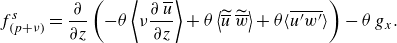
Distribution of the superficially double-averaged drag on the sediment bed. The coloured curves with symbols represent the drag-distribution obtained from the simulation (see (3.1)), while the dashed black lines represent the approximation by the fitting function using the case-specific fitting parameters $\mu _z$
and
$\mu _z$
and $\sigma _z$
(see (3.2)). Each of the three plots summarises simulation cases with an equal
$\sigma _z$
(see (3.2)). Each of the three plots summarises simulation cases with an equal $h/D$
ratio. The sphere diameter
$h/D$
ratio. The sphere diameter $D$
and the shear velocity
$D$
and the shear velocity $u_\tau$
are used for normalisation. Figure adapted from v.Wenczowski & Manhart (Reference v.Wenczowski and Manhart2024).
$u_\tau$
are used for normalisation. Figure adapted from v.Wenczowski & Manhart (Reference v.Wenczowski and Manhart2024).
While the nominal parameters of the simulation cases in table 1 refer to the geometrically defined interface, table 2 provides the interface-adapted flow depths and Reynolds numbers. For the computation of the interface-adapted Reynolds numbers, a consistent friction velocity is used, which is obtained as $u_\tau ^\mu = \sqrt {g_x h^\mu }$
. Whereas the Reynolds numbers of cases with smooth impermeable walls do not change, it is worthwhile to note that
$u_\tau ^\mu = \sqrt {g_x h^\mu }$
. Whereas the Reynolds numbers of cases with smooth impermeable walls do not change, it is worthwhile to note that $Re_\tau ^\mu \lt Re_\tau$
and
$Re_\tau ^\mu \lt Re_\tau$
and $Re_K^\mu \lt Re_K$
for cases with rough and permeable surfaces.
$Re_K^\mu \lt Re_K$
for cases with rough and permeable surfaces.
In the following, the vertical position is either specified in terms of $z/D$
or
$z/D$
or $z/h$
, where
$z/h$
, where $z$
refers to the geometrically defined interface. Alternatively to
$z$
refers to the geometrically defined interface. Alternatively to $z/h$
, we use the interface-adapted coordinate
$z/h$
, we use the interface-adapted coordinate $\zeta = (z - \mu _z) / (h - \mu _z)$
for orientation in the free-flow region, where
$\zeta = (z - \mu _z) / (h - \mu _z)$
for orientation in the free-flow region, where $\zeta = 0$
coincides with the drag-based interface and
$\zeta = 0$
coincides with the drag-based interface and $\zeta = 1$
with the free-slip water surface.
$\zeta = 1$
with the free-slip water surface.
In v.Wenczowski & Manhart (Reference v.Wenczowski and Manhart2024), we demonstrated that the flow-dynamically motivated drag-based interface and the adapted parameters allow us to unravel several similarities in the flow field, which we could not see clearly within the framework of the geometric interface. Particularly in advection-dominated regions, it appears unlikely to find potential similarities in the scalar field if there are no similarities in the flow field, such that we resort to the drag-based interface whenever we aim to investigate similarities. While we will employ the drag-based interface framework in parts where similarities are addressed, other paragraphs can be presented more conveniently with respect to the geometric interface.
3.5. Numerical methods
To resolve all temporal and spatial scales both in the free-flow region and in the pores of the sphere pack, we follow a single-domain DNS approach, which avoids model assumptions. The simulations were conducted by means of our MPI-parallel in-house code MGLET (Manhart, Tremblay & Friedrich Reference Manhart, Tremblay, Friedrich, Jenssen, Andersson, Ecer, Satofuka, Kvamsdal, Pettersen, Periaux and Fox2001; Manhart Reference Manhart2004; Sakai et al. Reference Sakai, Mendez, Strandenes, Ohlerich, Pasichnyk, Allalen and Manhart2019), which solves the incompressible Navier–Stokes equations using an energy-conserving central second-order finite-volume method. MGLET resorts to an explicit third-order low-storage Runge–Kutta method (Williamson Reference Williamson1980) for the time integration. Local grid refinement was applied to ensure that the Kolmogorov and Batchelor scales are resolved within the complete domain. The highest spatial resolution is required near the surface of the sediment bed, where we use cubic cells with a side length of $\Delta x_i^+ \lesssim 1$
(see table 1). Within the porous medium, a resolution of 48 cells per sphere diameter was found to yield a good resolution of the pore space (v.Wenczowski & Manhart Reference v.Wenczowski and Manhart2024). The geometry of the sphere pack is represented by an immersed boundary method. The no-slip Dirichlet condition on the sphere surfaces is enforced by a ghost-cell approach, which reaches second-order spatial accuracy for the velocity field, while mass conservation is ensured (Peller et al. Reference Peller, Duc, Tremblay and Manhart2006; Peller Reference Peller2010). The zero-flux Neumann boundary condition for the scalar reaches first-order spatial accuracy at the immersed boundary. By its construction, the implementation ensures strict conservation of the scalar within the complex geometry, such that we tolerate the reduced order in comparison to the velocity field. Commonly used spatial discretisation methods fail to resolve the infinitesimally narrow fluid gap at the contact points between spheres (Finn & Apte Reference Finn and Apte2013; Unglehrt & Manhart Reference Unglehrt and Manhart2022). To achieve a convergence against a defined geometry, we insert small fillet bridges, which seal regions where the sphere surfaces are extremely close to each other (v.Wenczowski & Manhart Reference v.Wenczowski and Manhart2024). We acknowledge that the contact points influence the mixing processes on the microscale (e.g. Heyman et al. Reference Heyman, Lester, Turuban, Méheust and Le Borgne2020), but, as errors cannot be completely avoided, it appears preferable to commit a quantifiable error, which is independent of the grid resolution.
$\Delta x_i^+ \lesssim 1$
(see table 1). Within the porous medium, a resolution of 48 cells per sphere diameter was found to yield a good resolution of the pore space (v.Wenczowski & Manhart Reference v.Wenczowski and Manhart2024). The geometry of the sphere pack is represented by an immersed boundary method. The no-slip Dirichlet condition on the sphere surfaces is enforced by a ghost-cell approach, which reaches second-order spatial accuracy for the velocity field, while mass conservation is ensured (Peller et al. Reference Peller, Duc, Tremblay and Manhart2006; Peller Reference Peller2010). The zero-flux Neumann boundary condition for the scalar reaches first-order spatial accuracy at the immersed boundary. By its construction, the implementation ensures strict conservation of the scalar within the complex geometry, such that we tolerate the reduced order in comparison to the velocity field. Commonly used spatial discretisation methods fail to resolve the infinitesimally narrow fluid gap at the contact points between spheres (Finn & Apte Reference Finn and Apte2013; Unglehrt & Manhart Reference Unglehrt and Manhart2022). To achieve a convergence against a defined geometry, we insert small fillet bridges, which seal regions where the sphere surfaces are extremely close to each other (v.Wenczowski & Manhart Reference v.Wenczowski and Manhart2024). We acknowledge that the contact points influence the mixing processes on the microscale (e.g. Heyman et al. Reference Heyman, Lester, Turuban, Méheust and Le Borgne2020), but, as errors cannot be completely avoided, it appears preferable to commit a quantifiable error, which is independent of the grid resolution.
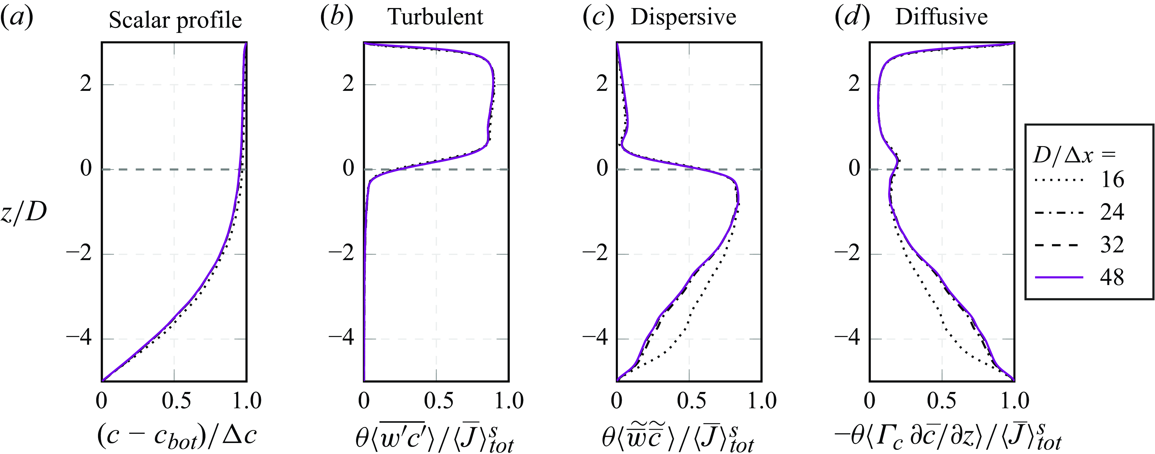
3.6. Convergence study
A case-specific grid study of the turbulent velocity field is documented in v.Wenczowski & Manhart (Reference v.Wenczowski and Manhart2024). This allows us to focus on the grid convergence of scalar profiles and the scalar transport processes, whereas turbulent and dispersive transport implicitly reflect the influence of the velocity field. The grid study is carried out on case L-180, which is the computationally cheapest simulation. Spatial resolutions with 16, 24, 32 and 48 cells per sphere diameter $D$
are compared. Figure 6 shows that the grid dependence is largest in deeper sediment layers, where insufficiently resolved configurations tend to underpredict diffusive scalar transport, while overpredicting the relative importance of dispersive transport.
$D$
are compared. Figure 6 shows that the grid dependence is largest in deeper sediment layers, where insufficiently resolved configurations tend to underpredict diffusive scalar transport, while overpredicting the relative importance of dispersive transport.
Grid study for case L-180. The scalar concentration profile (a) and the relative contributions of different transport processes to the total scalar flux (b–d) are evaluated for different grids with cubic cells of side length $\Delta x$
. The side length
$\Delta x$
. The side length $\Delta x$
is normalised by the sphere diameter
$\Delta x$
is normalised by the sphere diameter $D$
. A resolution of
$D$
. A resolution of $D/\Delta x=48$
corresponds to
$D/\Delta x=48$
corresponds to $\Delta x_i^+=1.21$
.
$\Delta x_i^+=1.21$
.
Statistical convergence study for case L-180. Besides the scalar concentration profile (a), relative contributions of different transport processes to the total scalar flux (b–d) are evaluated after different statistical sampling time spans $T_s$
. The sampling time span is normalised by the friction velocity
$T_s$
. The sampling time span is normalised by the friction velocity $u_\tau$
and the flow depth
$u_\tau$
and the flow depth $h$
.
$h$
.
In the flow case under consideration, the molecular scalar diffusion in the sediment bed is characterised by the largest time scale, which makes it the ‘slowest’ among all physical processes involved. Accordingly, the scalar field also requires more simulated time to reach a statistically stationary state than the velocity field. Due to that, the sampling of quantities related to scalar transport was only initiated a while after the sampling of velocity data had started. As a result, the scalar statistics were gathered over $T_s u_b / L_x \gt 10$
, which corresponds to
$T_s u_b / L_x \gt 10$
, which corresponds to $T_s u_\tau / h \gt 13$
. Thus, the scalar sampling time period
$T_s u_\tau / h \gt 13$
. Thus, the scalar sampling time period $T_s$
is about half as long as the sampling period
$T_s$
is about half as long as the sampling period $T$
of the velocity field (v.Wenczowski & Manhart Reference v.Wenczowski and Manhart2024). Using case L-180 as an example, the statistical convergence study in figure 7 shows a fast statistical convergence in the near-interface region, where turbulent motion on smaller length scales and shorter time scales is expected. In comparison, absolute statistical convergence in the free-flow region requires longer statistical sampling periods, whereas the time span
$T$
of the velocity field (v.Wenczowski & Manhart Reference v.Wenczowski and Manhart2024). Using case L-180 as an example, the statistical convergence study in figure 7 shows a fast statistical convergence in the near-interface region, where turbulent motion on smaller length scales and shorter time scales is expected. In comparison, absolute statistical convergence in the free-flow region requires longer statistical sampling periods, whereas the time span $T_s$
appears to be just sufficient for the convergence of second-order statistics.
$T_s$
appears to be just sufficient for the convergence of second-order statistics.
4. Results
The following § 4.1 provides an overview of the scalar concentration profiles under different normalisation. Similarities in the free-flow region scalar concentration profile (§ 4.2) can be traced back to a similarity in the effective diffusivity, as shown in § 4.3. Section 4.4 presents the dominant processes within different regions. Local hotspots of different transport processes are identified in § 4.5. Finally, § 4.6 focuses on the near-interface interaction between dispersive and turbulent transport.
4.1. Double-averaged scalar concentration profiles
The three plots in figure 8 show the intrinsically double-averaged scalar concentration $\langle \overline {c} \rangle$
under different normalisations. In figure 8(a) the concentration profile is normalised by the concentration difference
$\langle \overline {c} \rangle$
under different normalisations. In figure 8(a) the concentration profile is normalised by the concentration difference $\Delta c = c_{\textit{top}} - c_{\textit{bot}}$
. Accordingly, the obtained curves show a zero value at the bottom boundary and increase monotonically, until they reach a value of unity at the top domain boundary. The vertical coordinate
$\Delta c = c_{\textit{top}} - c_{\textit{bot}}$
. Accordingly, the obtained curves show a zero value at the bottom boundary and increase monotonically, until they reach a value of unity at the top domain boundary. The vertical coordinate $z$
is normalised by the sphere diameter
$z$
is normalised by the sphere diameter $D$
. Whilst all domains have the same depth of
$D$
. Whilst all domains have the same depth of $5 \, D$
, the top domain boundary is found at different heights in terms of
$5 \, D$
, the top domain boundary is found at different heights in terms of $z/D$
. The gradient of the double-averaged concentration profile differs drastically between the free-flow region and the sediment bed. In the free-flow region a small gradient
$z/D$
. The gradient of the double-averaged concentration profile differs drastically between the free-flow region and the sediment bed. In the free-flow region a small gradient $\partial \langle \overline {c} \rangle / \partial z$
suffices to maintain the bed-normal scalar flux, which hints at a high effective conductivity in this region. Within the sediment bed, a critically steeper concentration gradient indicates that the vertical scalar flux encounters a high resistance. For cases with low
$\partial \langle \overline {c} \rangle / \partial z$
suffices to maintain the bed-normal scalar flux, which hints at a high effective conductivity in this region. Within the sediment bed, a critically steeper concentration gradient indicates that the vertical scalar flux encounters a high resistance. For cases with low $Re_K$
, the profiles are approximately linear in the region of
$Re_K$
, the profiles are approximately linear in the region of $z/D \lt 0$
, whereas increasing values of
$z/D \lt 0$
, whereas increasing values of $Re_K$
lead to a progressively stronger curvature in the profiles below the interface, which points at a variation of the effective conductivity over the depth of the sediment bed. In figure 8(b) the vertical coordinate
$Re_K$
lead to a progressively stronger curvature in the profiles below the interface, which points at a variation of the effective conductivity over the depth of the sediment bed. In figure 8(b) the vertical coordinate $z$
is normalised by the flow depth
$z$
is normalised by the flow depth $h$
, which allows us to include the cases with smooth and impermeably bottom boundaries. Under normalisation with
$h$
, which allows us to include the cases with smooth and impermeably bottom boundaries. Under normalisation with $\Delta c$
, the concentration profiles deviate considerably from each other, as the scalar concentration at the geometrically defined interface at
$\Delta c$
, the concentration profiles deviate considerably from each other, as the scalar concentration at the geometrically defined interface at $z/D=0$
differs between the cases. This observation motivates the normalisation applied in figure 8(c), where the concentration at
$z/D=0$
differs between the cases. This observation motivates the normalisation applied in figure 8(c), where the concentration at $z=0$
acts as a reference. Under this normalisation, the profiles in the free-flow region have a similar shape, though they still do not collapse.
$z=0$
acts as a reference. Under this normalisation, the profiles in the free-flow region have a similar shape, though they still do not collapse.
Double-averaged scalar concentration profiles under different normalisations. (a) Scalar concentration normalised by the concentration difference between the bottom and top of the domain, i.e. $\Delta c = c_{\textit{top}} - c_{\textit{bot}}$
, and coordinate
$\Delta c = c_{\textit{top}} - c_{\textit{bot}}$
, and coordinate $z$
normalised by the sphere diameter
$z$
normalised by the sphere diameter $D$
, such that the top domain boundary is found at
$D$
, such that the top domain boundary is found at $z/D=3$
,
$z/D=3$
, $z/D=5$
or
$z/D=5$
or $z/D=10$
for L, M and S cases, respectively. (b) Normalisation of concentration profile like (a), but
$z/D=10$
for L, M and S cases, respectively. (b) Normalisation of concentration profile like (a), but $z$
normalised by the flow depth
$z$
normalised by the flow depth $h$
. Accordingly, the bottom domain boundary is found at
$h$
. Accordingly, the bottom domain boundary is found at $z/h = -1.67$
,
$z/h = -1.67$
, $z/h = -1$
or
$z/h = -1$
or $z/h = -0.5$
for L, M and S cases, respectively. (c) Concentration profile normalised by
$z/h = -0.5$
for L, M and S cases, respectively. (c) Concentration profile normalised by $c_{\textit{top}} - \langle \overline {c} \rangle _{(z=0)}$
, whereas the double-averaged concentration at
$c_{\textit{top}} - \langle \overline {c} \rangle _{(z=0)}$
, whereas the double-averaged concentration at $z=0$
is a reference. The coordinate
$z=0$
is a reference. The coordinate $z$
is normalised by
$z$
is normalised by $h$
.
$h$
.

4.2. Similarities in the free-flow region
To explore similarities in the free-flow scalar concentration profiles among all simulated cases, we resort to the dimensionless quantity $\langle { \overline {c} }\rangle ^+$
, which is defined as
$\langle { \overline {c} }\rangle ^+$
, which is defined as
 \begin{equation} \left \langle { \overline {c} }\right \rangle ^+ = \frac { \left \langle { \overline {c} }\right \rangle }{ c_\tau } , \quad \quad \text{with} \quad c_\tau = \frac { \langle \overline {J} \rangle ^s_{\textit{tot}} }{ u_\tau ^\mu } \quad \text{and} \quad u_\tau ^\mu = \sqrt { g_x h^\mu } . \end{equation}
The variable $c_\tau$
in (4.1) represents the friction scalar concentration (in analogy to the friction temperature), which is computed from the superficially double-averaged total scalar flux
$c_\tau$
in (4.1) represents the friction scalar concentration (in analogy to the friction temperature), which is computed from the superficially double-averaged total scalar flux $\langle \overline {J} \rangle _{\textit{tot}}^s$
in the bed-normal direction and the friction velocity
$\langle \overline {J} \rangle _{\textit{tot}}^s$
in the bed-normal direction and the friction velocity $u_\tau ^\mu$
. The friction velocity is obtained via a balance between the driving volume force and the wall friction, which includes the interface-adapted flow depth
$u_\tau ^\mu$
. The friction velocity is obtained via a balance between the driving volume force and the wall friction, which includes the interface-adapted flow depth $h^\mu$
(see (4.1)). In figure 9 the scalar concentration profiles are shown in a defect form, which exploits the prescribed fixed concentration value
$h^\mu$
(see (4.1)). In figure 9 the scalar concentration profiles are shown in a defect form, which exploits the prescribed fixed concentration value $c_{\textit{top}}$
at the clearly defined top domain boundary. The distance above the sediment is given relative to the flow depth under consideration of the interface position at
$c_{\textit{top}}$
at the clearly defined top domain boundary. The distance above the sediment is given relative to the flow depth under consideration of the interface position at $z = \mu _z$
. Above a certain distance from the bed surface, the dimensionless scalar defect profiles for cases with similar
$z = \mu _z$
. Above a certain distance from the bed surface, the dimensionless scalar defect profiles for cases with similar $Re_\tau$
collapse well, indicating an outer-layer similarity of the scalar field.
$Re_\tau$
collapse well, indicating an outer-layer similarity of the scalar field.
Defect representation of the dimensionless double-averaged concentration field. The concentration $c_{\textit{top}}$
is prescribed at the top domain boundary. The dimensionless vertical coordinate
$c_{\textit{top}}$
is prescribed at the top domain boundary. The dimensionless vertical coordinate $\zeta$
accounts for the drag-based interface position
$\zeta$
accounts for the drag-based interface position $\mu _z$
.
$\mu _z$
.
4.3. Effective diffusivity
The observed similarity under consideration of the total scalar flux also hints at a similarity of the effective scalar diffusivity among cases with similar $Re_\tau$
. Therefore, figure 10 provides profiles of the effective diffusivity, which is set in relation to the molecular diffusivity of the scalar. This ratio of
$Re_\tau$
. Therefore, figure 10 provides profiles of the effective diffusivity, which is set in relation to the molecular diffusivity of the scalar. This ratio of $\Gamma _{\textit{eff}} / \Gamma _c$
can be interpreted as a local Sherwood number for a differentially thin slice at a certain
$\Gamma _{\textit{eff}} / \Gamma _c$
can be interpreted as a local Sherwood number for a differentially thin slice at a certain $z$
position. Near the sediment--water interface, the profiles appear to group roughly according to the nominal permeability Reynolds numbers, as high values of
$z$
position. Near the sediment--water interface, the profiles appear to group roughly according to the nominal permeability Reynolds numbers, as high values of $Re_K$
are correlated with higher values of
$Re_K$
are correlated with higher values of $\Gamma _{\textit{eff}} / \Gamma _c$
. In the free-flow region the expected grouping according to
$\Gamma _{\textit{eff}} / \Gamma _c$
. In the free-flow region the expected grouping according to $Re_\tau$
is recognisable, whilst differences become most visible in the peak values around
$Re_\tau$
is recognisable, whilst differences become most visible in the peak values around $\zeta \approx 0.5$
.
$\zeta \approx 0.5$
.
Effective scalar diffusivity profile in the free-flow region. The effective diffusivity $\Gamma _{\textit{eff}}$
is normalised by the molecular diffusivity
$\Gamma _{\textit{eff}}$
is normalised by the molecular diffusivity $\Gamma _{\text{c}}$
. The dimensionless vertical coordinate
$\Gamma _{\text{c}}$
. The dimensionless vertical coordinate $\zeta$
accounts for the drag-based interface position
$\zeta$
accounts for the drag-based interface position $\mu _z$
.
$\mu _z$
.

To investigate the scaling behaviour in detail, figure 11(a) shows the effective diffusivity at the drag-based interface as a multiple of the molecular scalar diffusivity. The values are plotted over the interface-adapted permeability Reynolds number $Re_K^\mu$
. In addition, the dashed reference line represents the values predicted by the model of Voermans et al. (Reference Voermans, Ghisalberti and Ivey2018). The model provides separate expressions for the dispersive regime (
$Re_K^\mu$
. In addition, the dashed reference line represents the values predicted by the model of Voermans et al. (Reference Voermans, Ghisalberti and Ivey2018). The model provides separate expressions for the dispersive regime ( $Re_K \lt 1$
) and the turbulent regime (
$Re_K \lt 1$
) and the turbulent regime ( $Re_K \gt 1$
), which we evaluate for
$Re_K \gt 1$
), which we evaluate for $Sc = 1$
. Whereas the model prediction captures the macroscopic trend reasonably well, it underpredicts the numerically obtained effective diffusivity for low
$Sc = 1$
. Whereas the model prediction captures the macroscopic trend reasonably well, it underpredicts the numerically obtained effective diffusivity for low $Re_K$
. According to the model of Voermans et al. (Reference Voermans, Ghisalberti and Ivey2018), the diffusive regime with
$Re_K$
. According to the model of Voermans et al. (Reference Voermans, Ghisalberti and Ivey2018), the diffusive regime with $\Gamma _{\textit{eff}} / \Gamma _c = 1$
is only reached for
$\Gamma _{\textit{eff}} / \Gamma _c = 1$
is only reached for $Re_K \lt 0.02$
. In contrast to that, our data points suggest that
$Re_K \lt 0.02$
. In contrast to that, our data points suggest that $\Gamma _{\textit{eff}} / \Gamma _c \approx 1$
is already observed for case S-150. As discussed later in § 5, this observation can be linked to different Schmidt numbers. Figure 11(b) shows the scaling behaviour of the effective diffusivity in the centre of the free-flow region, i.e. at
$\Gamma _{\textit{eff}} / \Gamma _c \approx 1$
is already observed for case S-150. As discussed later in § 5, this observation can be linked to different Schmidt numbers. Figure 11(b) shows the scaling behaviour of the effective diffusivity in the centre of the free-flow region, i.e. at $\zeta = 0.5$
. The value of
$\zeta = 0.5$
. The value of $\Gamma _{\textit{eff}} / \Gamma _c$
increases linearly with respect to the interface-adapted friction Reynolds number
$\Gamma _{\textit{eff}} / \Gamma _c$
increases linearly with respect to the interface-adapted friction Reynolds number $Re_\tau ^\mu = u_\tau ^\mu h^\mu / \nu$
. From that, one can deduce that
$Re_\tau ^\mu = u_\tau ^\mu h^\mu / \nu$
. From that, one can deduce that ${\Gamma _{\textit{eff}}(\eta =0.5) } \approx 0.1 \, u_\tau ^\mu \, h^\mu$
, which means that the effective diffusivity in the free-flow region scales with the same interface-adapted velocity and length scales as the velocity field (v.Wenczowski & Manhart Reference v.Wenczowski and Manhart2024).
${\Gamma _{\textit{eff}}(\eta =0.5) } \approx 0.1 \, u_\tau ^\mu \, h^\mu$
, which means that the effective diffusivity in the free-flow region scales with the same interface-adapted velocity and length scales as the velocity field (v.Wenczowski & Manhart Reference v.Wenczowski and Manhart2024).
Scaling of the effective diffusivity $\Gamma _{\textit{eff}}$
at the drag-based interface at
$\Gamma _{\textit{eff}}$
at the drag-based interface at $\zeta = 0$
, i.e.
$\zeta = 0$
, i.e. $z=\mu _z$
, and in the centre of the free-flow region, i.e.
$z=\mu _z$
, and in the centre of the free-flow region, i.e. $\zeta = 0.5$
. The effective diffusivity is normalised by the molecular scalar diffusivity
$\zeta = 0.5$
. The effective diffusivity is normalised by the molecular scalar diffusivity $\Gamma _c$
. The adapted Reynolds numbers
$\Gamma _c$
. The adapted Reynolds numbers $Re_\tau ^\mu$
and
$Re_\tau ^\mu$
and $Re_K^\mu$
account for the drag-based interface. In (a) the relation according to Voermans et al. (Reference Voermans, Ghisalberti and Ivey2018) is given as a reference (dashed line). This relation includes a transition from a ‘dispersive’ to a ‘turbulent’ regime at
$Re_K^\mu$
account for the drag-based interface. In (a) the relation according to Voermans et al. (Reference Voermans, Ghisalberti and Ivey2018) is given as a reference (dashed line). This relation includes a transition from a ‘dispersive’ to a ‘turbulent’ regime at $Re_K \approx 1$
, which is marked in grey.
$Re_K \approx 1$
, which is marked in grey.
For modelling, the turbulent Schmidt number $Sc_t = \nu _t / \Gamma _t$
is a relevant parameter, as it represents the ratio between turbulent effective viscosity
$Sc_t = \nu _t / \Gamma _t$
is a relevant parameter, as it represents the ratio between turbulent effective viscosity $\nu _t = \langle \overline {u' w'} \rangle / \langle \partial \overline {u} / \partial z \rangle$
and the turbulent effective diffusivity
$\nu _t = \langle \overline {u' w'} \rangle / \langle \partial \overline {u} / \partial z \rangle$
and the turbulent effective diffusivity $\Gamma _t = \langle \overline {c' w'} \rangle / \langle \partial \overline {c} / \partial z \rangle$
. As shown in figure 12, the turbulent Schmidt number has a nearly constant value of slightly less than unity over large parts of the free-flow region, which agrees with previous studies (e.g. Schwertfirm & Manhart Reference Schwertfirm and Manhart2007; Pirozzoli, Bernardini & Orlandi Reference Pirozzoli, Bernardini and Orlandi2016). However,
$\Gamma _t = \langle \overline {c' w'} \rangle / \langle \partial \overline {c} / \partial z \rangle$
. As shown in figure 12, the turbulent Schmidt number has a nearly constant value of slightly less than unity over large parts of the free-flow region, which agrees with previous studies (e.g. Schwertfirm & Manhart Reference Schwertfirm and Manhart2007; Pirozzoli, Bernardini & Orlandi Reference Pirozzoli, Bernardini and Orlandi2016). However, $Sc_t$
deviates considerably from unity in regions influenced by the boundary conditions that are of different types for the scalar and the velocity field. In the region directly below the crests of the topmost spheres, i.e. near
$Sc_t$
deviates considerably from unity in regions influenced by the boundary conditions that are of different types for the scalar and the velocity field. In the region directly below the crests of the topmost spheres, i.e. near $0.5 \lt z/D \lt 1.0$
, the turbulent Schmidt number decreases. For the cases with high
$0.5 \lt z/D \lt 1.0$
, the turbulent Schmidt number decreases. For the cases with high $Re_K$
, it drops as low as
$Re_K$
, it drops as low as $Sc_{t, min} \approx 0.55$
, which qualitatively agrees with the findings of Chandesris et al. (Reference Chandesris, D’Hueppe, Mathieu, Jamet and Goyeau2013), who considered a critically more porous bed with
$Sc_{t, min} \approx 0.55$
, which qualitatively agrees with the findings of Chandesris et al. (Reference Chandesris, D’Hueppe, Mathieu, Jamet and Goyeau2013), who considered a critically more porous bed with $\theta = 0.875$
.
$\theta = 0.875$
.
Turbulent Schmidt number $Sc_t$
within the free-flow region. The dimensionless vertical coordinate
$Sc_t$
within the free-flow region. The dimensionless vertical coordinate $\zeta$
accounts for the drag-based interface position
$\zeta$
accounts for the drag-based interface position $\mu _z$
.
$\mu _z$
.
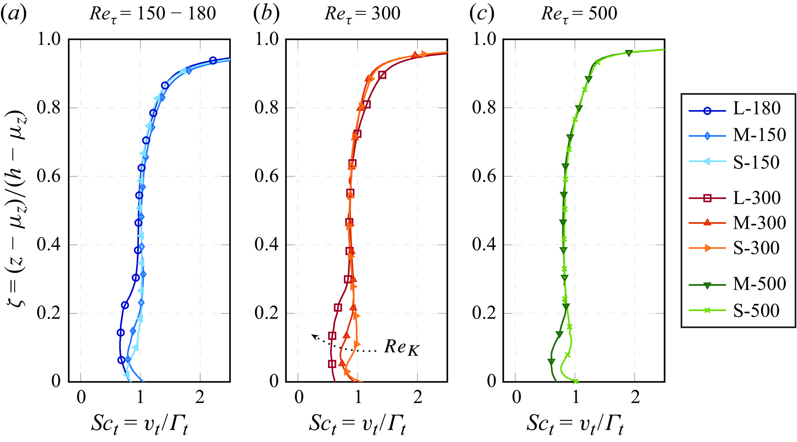
Relative contribution of different scalar transport processes to the total superficially averaged scalar flux $\langle \overline {J} \rangle ^s_{\textit{tot}}$
in the bed-normal direction. The dotted lines indicate the geometrically defined interface at
$\langle \overline {J} \rangle ^s_{\textit{tot}}$
in the bed-normal direction. The dotted lines indicate the geometrically defined interface at $z=0$
, whereas the dashed lines mark the drag-based interface position
$z=0$
, whereas the dashed lines mark the drag-based interface position $z = \mu _z$
for each case.
$z = \mu _z$
for each case.
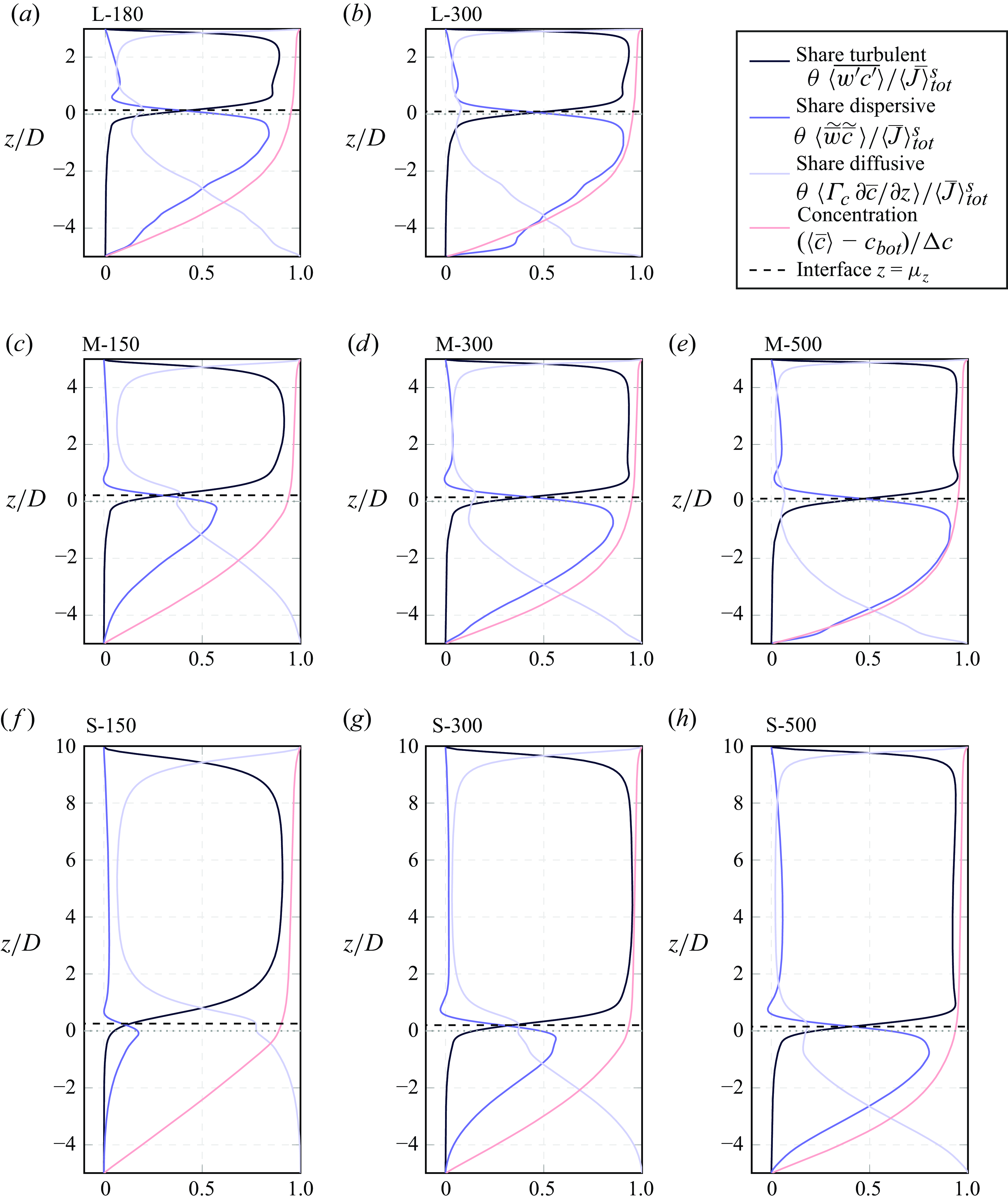
4.4. Scalar transport processes
The previous section has shown that the effective diffusivity of the scalar exceeds the molecular diffusivity by far, which implies that other non-Fickian transport processes contribute greatly to the total scalar flux $\langle \overline {J} \rangle _{\textit{tot}}$
. For each case separately, the plots in figure 13 show the relative contributions of turbulent, dispersive and diffusive transport to the total bed-normal scalar flux as a function of
$\langle \overline {J} \rangle _{\textit{tot}}$
. For each case separately, the plots in figure 13 show the relative contributions of turbulent, dispersive and diffusive transport to the total bed-normal scalar flux as a function of $z$
. At the free-slip top boundary of the domain, a thin layer exists where only diffusive scalar transport takes place in the absence of surface-normal fluid motion. Away from this diffusion-dominated layer, turbulent transport is dominant throughout the free-flow region. Around the position of
$z$
. At the free-slip top boundary of the domain, a thin layer exists where only diffusive scalar transport takes place in the absence of surface-normal fluid motion. Away from this diffusion-dominated layer, turbulent transport is dominant throughout the free-flow region. Around the position of $z \approx 0$
, however, the influence of turbulent transport declines drastically with decreasing
$z \approx 0$
, however, the influence of turbulent transport declines drastically with decreasing $z$
, while diffusive and dispersive quickly gain relevance. For the simulated cases with unity Schmidt number, the permeability Reynolds number seems to determine whether diffusive or dispersive transport is dominant. Only for case S-150 with
$z$
, while diffusive and dispersive quickly gain relevance. For the simulated cases with unity Schmidt number, the permeability Reynolds number seems to determine whether diffusive or dispersive transport is dominant. Only for case S-150 with $Re_K \approx 0.4$
, diffusive transport dominates over dispersive transport within the complete sediment bed. For
$Re_K \approx 0.4$
, diffusive transport dominates over dispersive transport within the complete sediment bed. For $Re_K \approx 0.8$
(e.g. cases M-150 and S-300), the contributions of both processes are approximately equal within the region directly below the sediment bed surface. With increasing
$Re_K \approx 0.8$
(e.g. cases M-150 and S-300), the contributions of both processes are approximately equal within the region directly below the sediment bed surface. With increasing $Re_K$
, dispersive transport finally dominates in the layer shortly below the sediment surface. Deeper inside the sediment bed, the contribution of dispersive transport fades out to the benefit of diffusive transport. Finally, diffusive transport is once again exclusively responsible for the scalar flux across the bottom domain boundary.
$Re_K$
, dispersive transport finally dominates in the layer shortly below the sediment surface. Deeper inside the sediment bed, the contribution of dispersive transport fades out to the benefit of diffusive transport. Finally, diffusive transport is once again exclusively responsible for the scalar flux across the bottom domain boundary.
The plots in figure 13 visualise that the decline of turbulent scalar transport and the increase in dispersive transport with decreasing $z$
happen within a relatively narrow region near the interface. Within this narrow region, the bed-normal scalar transport due to molecular diffusion reaches a local maximum, hinting at the presence of higher vertical concentration gradients. The elevation
$z$
happen within a relatively narrow region near the interface. Within this narrow region, the bed-normal scalar transport due to molecular diffusion reaches a local maximum, hinting at the presence of higher vertical concentration gradients. The elevation $z_{(\textit{turb=disp})}$
, at which the contributions of turbulent and dispersive transport are equally large, coincides fairly well with the position of the drag-based interface, which is found at
$z_{(\textit{turb=disp})}$
, at which the contributions of turbulent and dispersive transport are equally large, coincides fairly well with the position of the drag-based interface, which is found at $z = \mu _z$
. As shown by figure 14, both
$z = \mu _z$
. As shown by figure 14, both $z_{(\textit{turb=disp})}$
and
$z_{(\textit{turb=disp})}$
and $\mu _z$
decrease with increasing
$\mu _z$
decrease with increasing $Re_K$
, such that both approach the position of the geometrically defined interface. The grey dashed line is the same in both plots and provides a reference.
$Re_K$
, such that both approach the position of the geometrically defined interface. The grey dashed line is the same in both plots and provides a reference.
Transition between turbulent and dispersive transport at the interface. The position $z_{(\textit{turb=disp})}$
marks where the dispersive scalar flux equals the turbulent flux, i.e.
$z_{(\textit{turb=disp})}$
marks where the dispersive scalar flux equals the turbulent flux, i.e. $\langle J \rangle ^s_{\textit{disp}} = \langle J \rangle ^s_{\textit{turb}}$
, and is plotted over
$\langle J \rangle ^s_{\textit{disp}} = \langle J \rangle ^s_{\textit{turb}}$
, and is plotted over $Re_K$
. Similarly, the position
$Re_K$
. Similarly, the position $\mu _z$
of the drag-based interface is plotted over
$\mu _z$
of the drag-based interface is plotted over $Re_K$
. The dashed line marks a common trend.
$Re_K$
. The dashed line marks a common trend.
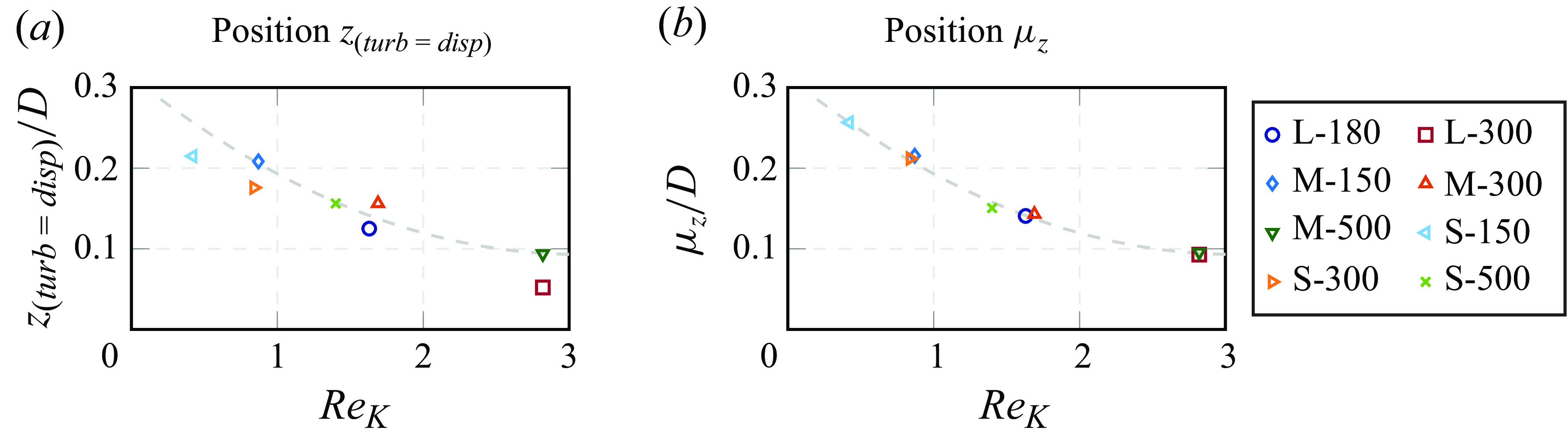
Figure 15 focuses on the near-interface region and compares all simulated cases. The grouping of curves corroborates the concept of Voermans et al. (Reference Voermans, Ghisalberti and Ivey2018), according to which $Re_K$
determines the dominant scalar transport processes. With increasing
$Re_K$
determines the dominant scalar transport processes. With increasing $Re_K$
, turbulent scalar transport can affect progressively deeper regions of the sediment bed. Deeper below the interface, however, the contribution of turbulent scalar transport tails out. This observation is contrasted by the dispersive transport, which gains maximal influence in the near-interface region and only decreases gradually in deeper regions. At the largest
$Re_K$
, turbulent scalar transport can affect progressively deeper regions of the sediment bed. Deeper below the interface, however, the contribution of turbulent scalar transport tails out. This observation is contrasted by the dispersive transport, which gains maximal influence in the near-interface region and only decreases gradually in deeper regions. At the largest $Re_K$
of our parameter space, nearly the complete scalar transport at
$Re_K$
of our parameter space, nearly the complete scalar transport at $z/D \approx -1$
is leveraged by dispersive transport. As the contributions of dispersive and turbulent transport increase at the interface, the relative share of transport due to molecular diffusion decreases at progressively higher
$z/D \approx -1$
is leveraged by dispersive transport. As the contributions of dispersive and turbulent transport increase at the interface, the relative share of transport due to molecular diffusion decreases at progressively higher $Re_K$
.
$Re_K$
.
Influence of the permeability Reynolds number $Re_K$
on the relative contributions of different scalar transport processes to the total scalar flux
$Re_K$
on the relative contributions of different scalar transport processes to the total scalar flux $\langle J \rangle ^s_{\textit{tot}}$
in the bed-normal direction. The curves group according to
$\langle J \rangle ^s_{\textit{tot}}$
in the bed-normal direction. The curves group according to $Re_K$
. The vertical coordinate
$Re_K$
. The vertical coordinate $z$
is normalised by the sphere diameter
$z$
is normalised by the sphere diameter $D$
. Note that the normalisation of a flux by
$D$
. Note that the normalisation of a flux by $\langle J \rangle ^s_{\textit{tot}}$
corresponds to a normalisation by
$\langle J \rangle ^s_{\textit{tot}}$
corresponds to a normalisation by $(u_\tau^\mu c_\tau )$
.
$(u_\tau^\mu c_\tau )$
.
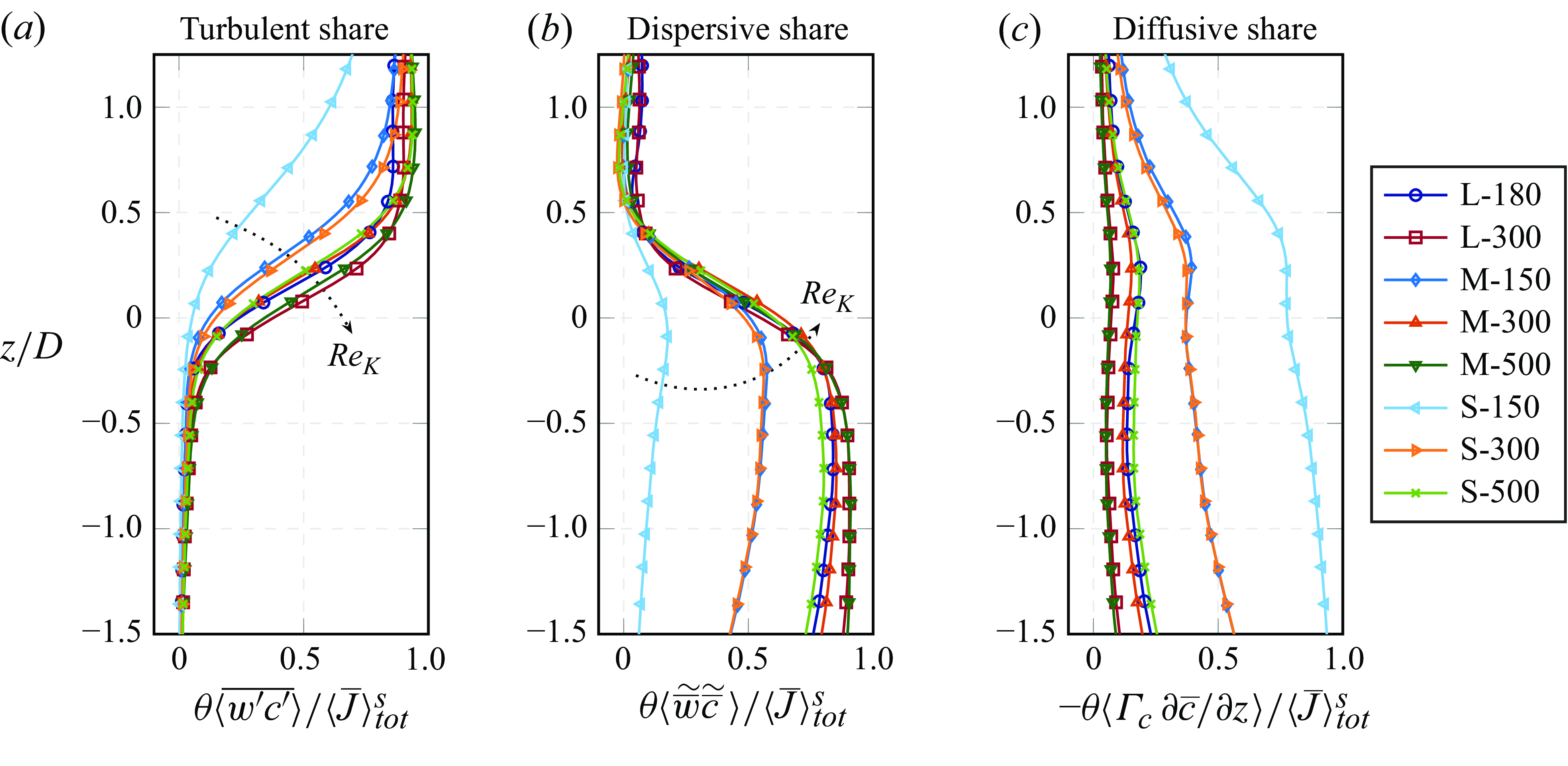
Process-specific effective diffusivity profiles for turbulent and dispersive scalar transport in the near-interface region. The effective diffusivity is normalised by the molecular diffusivity and the vertical coordinate $z$
by the sphere diameter
$z$
by the sphere diameter $D$
. The profiles tend to group according to
$D$
. The profiles tend to group according to $Re_K$
.
$Re_K$
.

In figure 15 the impact of different processes was evaluated in terms of their relative contribution to the total scalar flux. This representation may yield the impression that the sub-interface dispersive scalar transport is as effective as the turbulent transport in the free-flow region. Figure 16 corrects this impression by providing the process-specific effective diffusivities, which result from a comparison to the diffusive scalar transport. Above the sediment bed, the scalar field is well mixed, such that hardly any vertical concentration gradient is present, and the turbulent scalar transport achieves a higher effective diffusivity. In contrast, dispersive transport acts below the interface, where comparatively strong vertical scalar concentration gradients prevail, which exposes a lower effective diffusivity associated with the process. The near-interface turbulent effective diffusivity profiles collapse well for cases with similar $Re_K$
. In comparison, differences between the dispersive effective diffusivity profiles are larger. A possible reason could be that specific geometrical properties of the generated sediment beds have more impact on the dispersive transport.
$Re_K$
. In comparison, differences between the dispersive effective diffusivity profiles are larger. A possible reason could be that specific geometrical properties of the generated sediment beds have more impact on the dispersive transport.
Correlations between the bed-normal velocity $w$
and the scalar concentration
$w$
and the scalar concentration $c$
. Correlated spatial variations (a) are responsible for dispersive scalar transport. Correlated temporal fluctuations (b) are required for turbulent scalar transport. Each point represents a sample taken at a random position within the plane
$c$
. Correlated spatial variations (a) are responsible for dispersive scalar transport. Correlated temporal fluctuations (b) are required for turbulent scalar transport. Each point represents a sample taken at a random position within the plane $z=0$
of case M-500. The red colour indicates a positive contribution and the blue colour a negative contribution to the scalar transport.
$z=0$
of case M-500. The red colour indicates a positive contribution and the blue colour a negative contribution to the scalar transport.

4.5. Distribution of scalar transport processes in space
Dispersive transport requires a correlation between the spatial variations of the time averaged bed-normal velocity field and the scalar concentration field, whereas turbulent scalar transport requires a correlation of the temporal fluctuations of the two fields. The scatter plots in figure 17 visualise the quality of these correlations at the position $z=0$
of case M-500. Regions of downwelling time-averaged fluid motion through the interface are characterised by
$z=0$
of case M-500. Regions of downwelling time-averaged fluid motion through the interface are characterised by $\widetilde { \overline {w}} \lt 0$
. The samples in the third and fourth quadrant of figure 17(a) show that
$\widetilde { \overline {w}} \lt 0$
. The samples in the third and fourth quadrant of figure 17(a) show that $\widetilde { \overline {c}}$
is close to zero under these conditions, with only a slight tendency towards positive values. This suggests that downwelling motion at the geometrically defined interface transports fluid with a nearly uniform scalar concentration from the well-mixed free-flow region into the sediment bed. In contrast, the scalar concentration in the upwelling flow (
$\widetilde { \overline {c}}$
is close to zero under these conditions, with only a slight tendency towards positive values. This suggests that downwelling motion at the geometrically defined interface transports fluid with a nearly uniform scalar concentration from the well-mixed free-flow region into the sediment bed. In contrast, the scalar concentration in the upwelling flow ( $\widetilde { \overline {w}} \gt 0$
) varies over a much wider range. The scalar concentration in the free-flow region seems to impose an upper limit for positive
$\widetilde { \overline {w}} \gt 0$
) varies over a much wider range. The scalar concentration in the free-flow region seems to impose an upper limit for positive $\widetilde { \overline {c}}$
(see first quadrant). In some upwelling regions, however,
$\widetilde { \overline {c}}$
(see first quadrant). In some upwelling regions, however, $\widetilde { \overline {c}}$
has negative values of high amplitude, as shown by the circles in the second quadrant. At these sampled locations, fluid with scalar concentrations closer to
$\widetilde { \overline {c}}$
has negative values of high amplitude, as shown by the circles in the second quadrant. At these sampled locations, fluid with scalar concentrations closer to $c_{\textit{bot}}$
is transported upwards through the interface. A reason could be that individual nearly vertical flow paths exist that cross regions of high vertical concentration gradients and advect fluid from deeper layers upwards. For turbulent transport resulting from temporal fluctuations, however, similar observations cannot be made. As shown in figure 17(b), the negative correlation between
$c_{\textit{bot}}$
is transported upwards through the interface. A reason could be that individual nearly vertical flow paths exist that cross regions of high vertical concentration gradients and advect fluid from deeper layers upwards. For turbulent transport resulting from temporal fluctuations, however, similar observations cannot be made. As shown in figure 17(b), the negative correlation between $w^\prime$
and
$w^\prime$
and $c^\prime$
becomes mainly visible from a few points in the second and fourth quadrant. These observations suggest that dispersive and turbulent transport behave differently, which we will investigate further by analysing their distribution in space.
$c^\prime$
becomes mainly visible from a few points in the second and fourth quadrant. These observations suggest that dispersive and turbulent transport behave differently, which we will investigate further by analysing their distribution in space.
Local contributions to the turbulent, dispersive and diffusive scalar transport within an arbitrarily chosen $x$
--
$x$
-- $z$
-plane of simulation case M-500. The values are normalised by the absolute value of the superficially averaged total scalar flux
$z$
-plane of simulation case M-500. The values are normalised by the absolute value of the superficially averaged total scalar flux $\langle J \rangle ^s_{\textit{tot}}$
. Coordinates in the
$\langle J \rangle ^s_{\textit{tot}}$
. Coordinates in the $x$
- and
$x$
- and $z$
-direction are given in
$z$
-direction are given in $x/D$
and
$x/D$
and $z/D$
, respectively, where
$z/D$
, respectively, where $D$
is the sphere diameter.
$D$
is the sphere diameter.
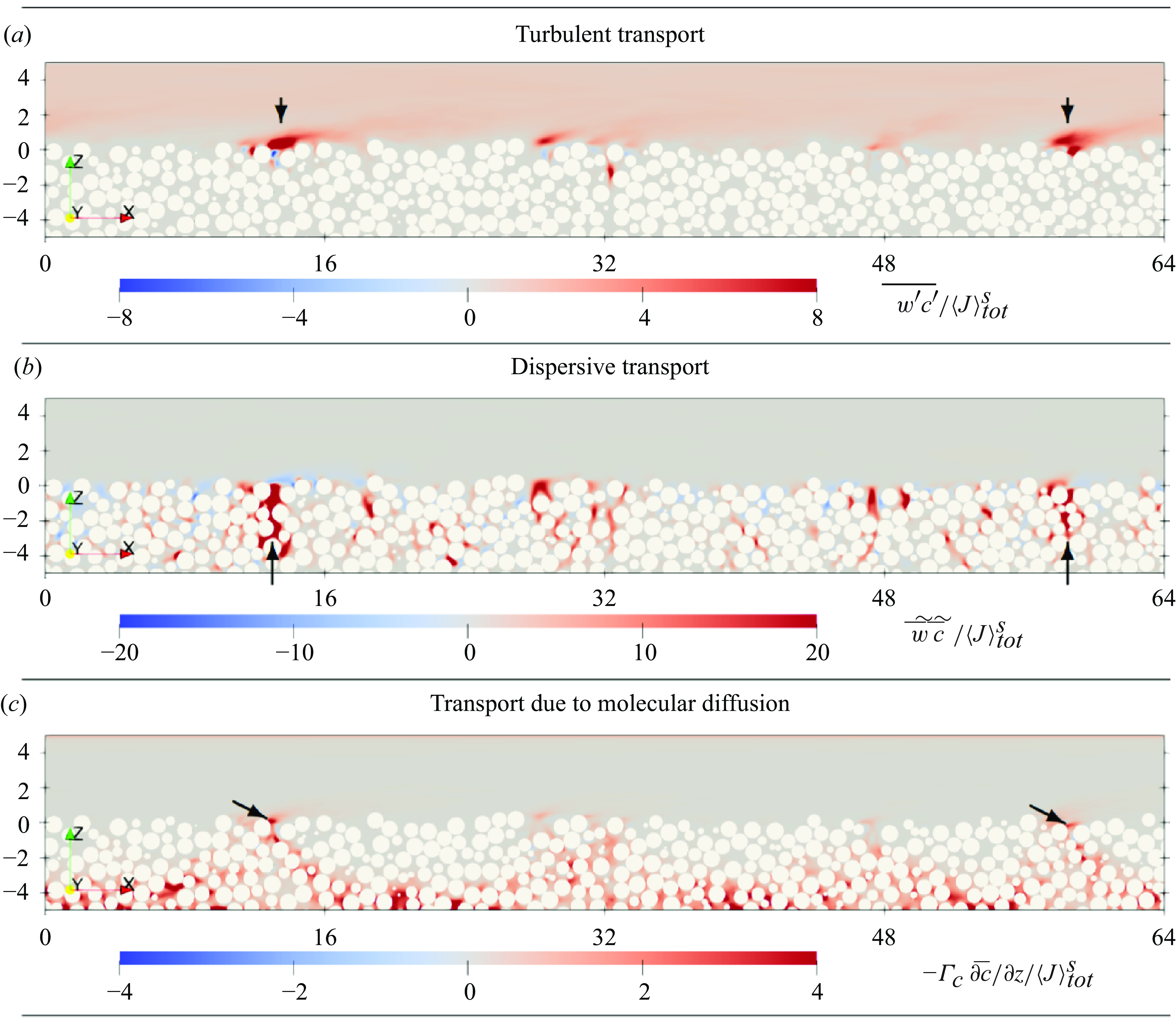
Figure 18 shows the local contributions to turbulent, dispersive and diffusive transport within an arbitrarily chosen vertical slice through case M-500. Above $z/D \approx 2$
, the turbulent scalar transport seems to occur nearly uniformly distributed in space, which suggests that this region is well mixed. Only at a few individual spots, turbulenttransport takes place within the pore space below the bed surface. In contrast, several local hotspots of increased bed-normal turbulent scalar transport are found directly above the sediment--water interface, e.g. at
$z/D \approx 2$
, the turbulent scalar transport seems to occur nearly uniformly distributed in space, which suggests that this region is well mixed. Only at a few individual spots, turbulenttransport takes place within the pore space below the bed surface. In contrast, several local hotspots of increased bed-normal turbulent scalar transport are found directly above the sediment--water interface, e.g. at $x/D \approx 14$
or
$x/D \approx 14$
or $x/D \approx 58$
in figure 18(a). The observations made in the arbitrarily chosen slice suggest that hotspots of turbulent scalar transport above the interface occur where upwelling fluid motion contributes strongly to enhanced dispersive transport below the sediment--water interface. In figure 18(b), two such locations are marked by arrows. In their appearance, these locations resemble chimneys, which release the scalar quantity. Continuing in this analogy, the transition from dispersive to turbulent transport near the interface represents the outlet of the sub-interface chimney, from which the released scalar is immediately advected downstream within the free-flow field. Due to this downstream advection, a strong vertical concentration gradient prevails at the chimney outlet, which fosters the local diffusive scalar transport. In figure 18(c), two such near-interface locations with local maxima of diffusive transport are marked by arrows.
$x/D \approx 58$
in figure 18(a). The observations made in the arbitrarily chosen slice suggest that hotspots of turbulent scalar transport above the interface occur where upwelling fluid motion contributes strongly to enhanced dispersive transport below the sediment--water interface. In figure 18(b), two such locations are marked by arrows. In their appearance, these locations resemble chimneys, which release the scalar quantity. Continuing in this analogy, the transition from dispersive to turbulent transport near the interface represents the outlet of the sub-interface chimney, from which the released scalar is immediately advected downstream within the free-flow field. Due to this downstream advection, a strong vertical concentration gradient prevails at the chimney outlet, which fosters the local diffusive scalar transport. In figure 18(c), two such near-interface locations with local maxima of diffusive transport are marked by arrows.
The insight from the local contributions to turbulent, dispersive and diffusive transport facilitates the interpretation of the double-averaged flux values, previously presented in figure 13. Accordingly, the sharp near-interface transition between dispersive and turbulent transport coincides with the outlets of the sub-interface chimneys. The enhanced diffusive transport at the chimney outlets explains the local maximum in the share of the diffusive scalar transport, which accompanies the transition between dispersive and turbulent transport. The abrupt transition at the chimney outlets also implies that there is hardly any spatial overlap between dispersive and turbulent scalar transport hotspots. Rather, one process replaces the other such that the local vertical scalar flux is continued across the interface.
4.6. Interaction at the interface
The previous sections have shown that different scalar transport processes are active in the near-interface region. In the following, we aim to describe their interaction both qualitatively and quantitatively. For the qualitative investigation, we consider the arbitrarily chosen vertical slice through case M-500, for which different quantities are provided in figure 19. Figure 19(a) shows the time-averaged scalar concentration field. Even with a strongly nonlinear colour map, hardly any concentration differences become visible in the well-mixed free-flow region. Strong scalar concentration gradients, however, prevail within the sediment bed. It is remarkable that isoconcentration surfaces in this region are not even approximately parallel to the surface of the sediment bed, but have a strong relief. For cases with lower $Re_K$
, this relief is not as strong, yet still present (not shown). Figure 19(b) shows a realisation of the instantaneous scalar concentration field. The strongly nonlinear colour map emphasises concentration differences in the free-flow region. In particular near the chimney outlets, the interaction between turbulent fluid motion and the scalar concentration field becomes visible and suggests enhanced turbulent mixing at these locations. One such location is marked by dashed boxed in figure 19(b). As formally shown by (2.10) and (2.11) in § 2.4, the form-induced production mechanism creates temporal scalar fluctuations, while reducing the spatial variance in the scalar field. Figure 19(c) corroborates that the marked location acts as one hotspot of form-induced production, while further hotspots are found around the chimneys at
$Re_K$
, this relief is not as strong, yet still present (not shown). Figure 19(b) shows a realisation of the instantaneous scalar concentration field. The strongly nonlinear colour map emphasises concentration differences in the free-flow region. In particular near the chimney outlets, the interaction between turbulent fluid motion and the scalar concentration field becomes visible and suggests enhanced turbulent mixing at these locations. One such location is marked by dashed boxed in figure 19(b). As formally shown by (2.10) and (2.11) in § 2.4, the form-induced production mechanism creates temporal scalar fluctuations, while reducing the spatial variance in the scalar field. Figure 19(c) corroborates that the marked location acts as one hotspot of form-induced production, while further hotspots are found around the chimneys at $x/D \approx 14$
or
$x/D \approx 14$
or $x/D \approx 58$
(not shown). The visualisation by volume rendering uses a logarithmic colour map, as regions of high form-induced production appear strongly localised. Most hotspots of form-induced production are found between the spheres in the topmost layer of the sediment bed. Below that, the local observation suggests that only a few spots of high form-induced production intensity occur primarily in larger pores, which are likely to provide good conditions for turbulent mixing. Apart from those local hotspots, hardly any form-induced production can be detected in large parts of the porous medium.
$x/D \approx 58$
(not shown). The visualisation by volume rendering uses a logarithmic colour map, as regions of high form-induced production appear strongly localised. Most hotspots of form-induced production are found between the spheres in the topmost layer of the sediment bed. Below that, the local observation suggests that only a few spots of high form-induced production intensity occur primarily in larger pores, which are likely to provide good conditions for turbulent mixing. Apart from those local hotspots, hardly any form-induced production can be detected in large parts of the porous medium.
Form-induced production of temporal scalar fluctuations. The mean scalar concentration field (a) and an instantaneous scalar concentration field (b) are shown within an arbitrarily chosen $x$
-
$x$
- $z$
-plane of simulation case M-500. The form-induced production (c) appears strongly localised with spots of strong intensity near the chimneys, of which one is marked by the dashed box. Coordinates in
$z$
-plane of simulation case M-500. The form-induced production (c) appears strongly localised with spots of strong intensity near the chimneys, of which one is marked by the dashed box. Coordinates in $x$
- and
$x$
- and $z$
-direction are given in
$z$
-direction are given in $x/D$
and
$x/D$
and $z/D$
, respectively, where
$z/D$
, respectively, where $D$
is the sphere diameter.
$D$
is the sphere diameter.
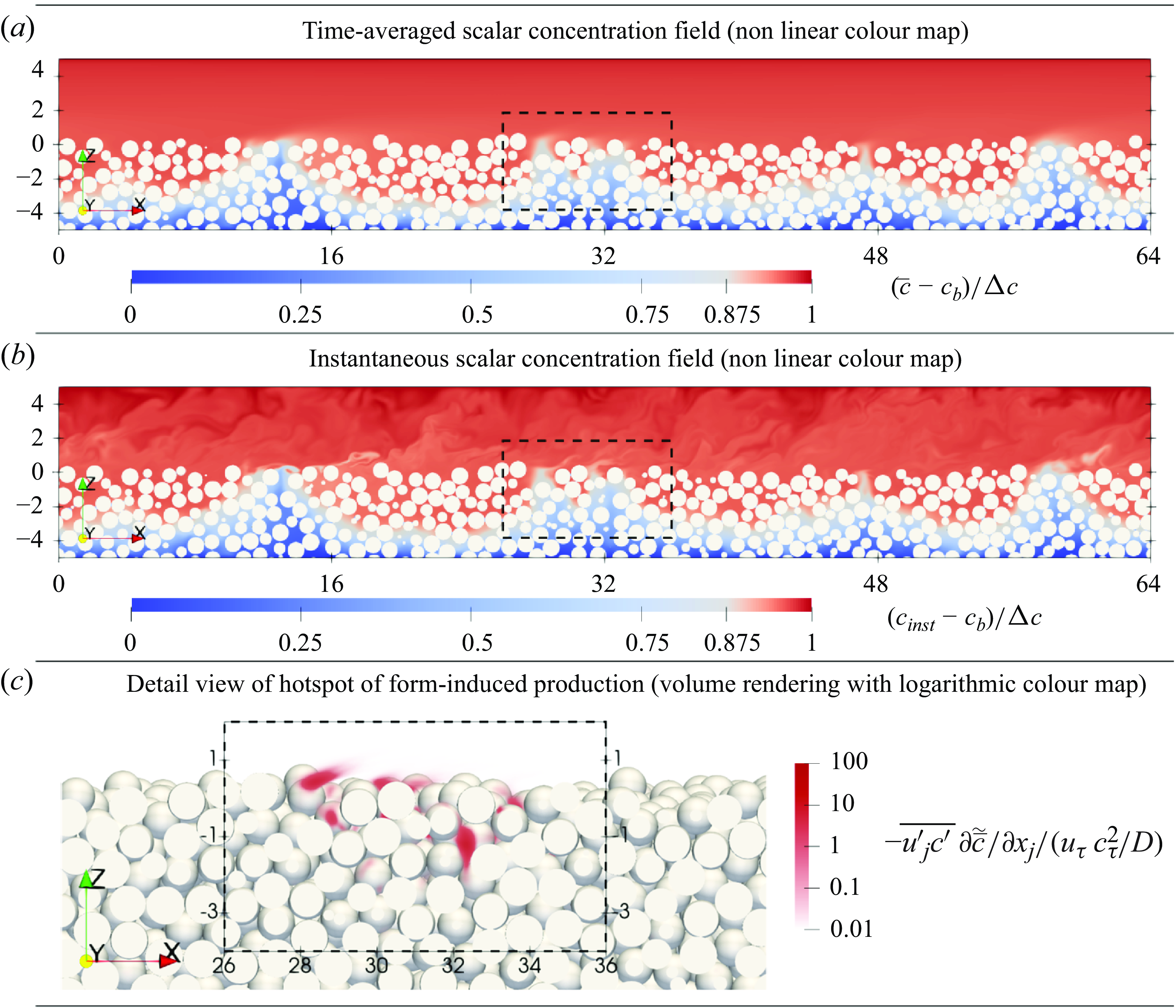
To assess the impact and the scaling behaviour of form-induced production, we evaluate double-averaged profiles. Figure 20(a) shows the profiles of form-induced production intensity, using the sphere diameter, the friction velocity and the friction scalar concentration value for a normalisation with interface-related scales. Except for S-150, all cases exhibit a form-induced production peak, which is found at $z/D \approx 0.5$
for lower
$z/D \approx 0.5$
for lower $Re_K$
and moves towards
$Re_K$
and moves towards $z/D \approx 0.2$
with increasing
$z/D \approx 0.2$
with increasing $Re_K$
. Under the given normalisation, the amplitude of the peak increases with
$Re_K$
. Under the given normalisation, the amplitude of the peak increases with $Re_K$
, causing the curves to group roughly accordingly. Below the peak, the form-induced production declines with increasing depth, whereas the tailing behaviour is similarly determined by
$Re_K$
, causing the curves to group roughly accordingly. Below the peak, the form-induced production declines with increasing depth, whereas the tailing behaviour is similarly determined by $Re_K$
. For cases with high
$Re_K$
. For cases with high $Re_K$
, the form-induced production introduces temporal scalar fluctuation even at greater depth. Most notably for case L-300, the profile is not fully smooth but exhibits characteristic features. This agrees with the observation that the form-induced production does not occur uniformly in space, but rather concentrates in certain locations. To put the influence of the form-induced production in relation, figure 20(b) shows the gradient production of scalar fluctuations. For all cases with
$Re_K$
, the form-induced production introduces temporal scalar fluctuation even at greater depth. Most notably for case L-300, the profile is not fully smooth but exhibits characteristic features. This agrees with the observation that the form-induced production does not occur uniformly in space, but rather concentrates in certain locations. To put the influence of the form-induced production in relation, figure 20(b) shows the gradient production of scalar fluctuations. For all cases with $Re_K \gt 1$
, the peak of the form-induced production is considerably larger than the peak value of the gradient production. A further difference to the form-induced production is that gradient production hardly affects the region
$Re_K \gt 1$
, the peak of the form-induced production is considerably larger than the peak value of the gradient production. A further difference to the form-induced production is that gradient production hardly affects the region $z/D \lt 0$
, whereas it does have influence in the free-flow region.
$z/D \lt 0$
, whereas it does have influence in the free-flow region.
Production mechanisms of temporal scalar fluctuations: profiles of form-induced production (a) and gradient production (b) in direct comparison. For normalisation, the friction velocity $u_\tau$
, the friction scalar concentration
$u_\tau$
, the friction scalar concentration $c_\tau = \langle \overline {J} \rangle _{\textit{tot}} / u_\tau$
and the sphere diameter
$c_\tau = \langle \overline {J} \rangle _{\textit{tot}} / u_\tau$
and the sphere diameter $D$
are used.
$D$
are used.

5. Discussion
The defect representation of the double-averaged concentration profiles reveals an outer-layer similarity among cases with similar $Re_\tau$
(figure 9). This similarity shows up under the normalisation
$Re_\tau$
(figure 9). This similarity shows up under the normalisation $\langle \overline {c} \rangle ^+ = { \langle \overline {c} \rangle \, u_\tau ^\mu } \, / \, { \langle \overline {J} \rangle ^s_{\textit{tot}} }$
, in which the flux compensates for different conditions in the bed and the friction velocity acts as a velocity scale. The similarity under consideration of the flux implies that the ratio between effective and molecular diffusivity, i.e.
$\langle \overline {c} \rangle ^+ = { \langle \overline {c} \rangle \, u_\tau ^\mu } \, / \, { \langle \overline {J} \rangle ^s_{\textit{tot}} }$
, in which the flux compensates for different conditions in the bed and the friction velocity acts as a velocity scale. The similarity under consideration of the flux implies that the ratio between effective and molecular diffusivity, i.e. $\Gamma _{\textit{eff}} / \Gamma _c$
, at a certain vertical position is determined by
$\Gamma _{\textit{eff}} / \Gamma _c$
, at a certain vertical position is determined by $Re_\tau$
or, even more accurately, by the interface-adapted Reynolds number
$Re_\tau$
or, even more accurately, by the interface-adapted Reynolds number $Re_\tau ^\mu$
(figure 11). The observations that
$Re_\tau ^\mu$
(figure 11). The observations that $\Gamma _{\textit{eff}}$
scales with
$\Gamma _{\textit{eff}}$
scales with $u_\tau ^\mu \, h^\mu$
and that the turbulent Schmidt number is near unity over large parts of the flow depth agree well with the findings of Pirozzoli et al. (Reference Pirozzoli, Bernardini and Orlandi2016) for smooth-wall channel flow. It has been observed in v.Wenczowski & Manhart (Reference v.Wenczowski and Manhart2024) that also the outer-layer velocity profiles and turbulent fields show similarities at similar
$u_\tau ^\mu \, h^\mu$
and that the turbulent Schmidt number is near unity over large parts of the flow depth agree well with the findings of Pirozzoli et al. (Reference Pirozzoli, Bernardini and Orlandi2016) for smooth-wall channel flow. It has been observed in v.Wenczowski & Manhart (Reference v.Wenczowski and Manhart2024) that also the outer-layer velocity profiles and turbulent fields show similarities at similar $Re_\tau$
, if the drag-based interface position is used. In our view, those similarities are tightly linked to the observed similarity of the concentration profiles in the outer layer, which is dominated by turbulent transport.
$Re_\tau$
, if the drag-based interface position is used. In our view, those similarities are tightly linked to the observed similarity of the concentration profiles in the outer layer, which is dominated by turbulent transport.
While the free-flow region is dominated by turbulent transport, different scalar transport regimes can be distinguished at the sediment--water interface. According to Voermans et al. (Reference Voermans, Ghisalberti and Ivey2018), the transition from the diffusive to the dispersive regime takes place at $Re_K \approx 0.02$
. For case S-150, which is characterised by
$Re_K \approx 0.02$
. For case S-150, which is characterised by $Re_K \approx 0.4$
, however, we already observe that molecular diffusion dominates the near-interface scalar transport (figure 15). This discrepancy may be explained by the role of the Schmidt number
$Re_K \approx 0.4$
, however, we already observe that molecular diffusion dominates the near-interface scalar transport (figure 15). This discrepancy may be explained by the role of the Schmidt number $Sc = \nu / \Gamma$
, which was set to unity in the present study. To avoid jumps in the predicted effective diffusivity between the diffusive regime (
$Sc = \nu / \Gamma$
, which was set to unity in the present study. To avoid jumps in the predicted effective diffusivity between the diffusive regime ( $D_{\textit{eff}} / \Gamma = 1$
for
$D_{\textit{eff}} / \Gamma = 1$
for $Re_K \lt 0.02$
) and the dispersive regime (
$Re_K \lt 0.02$
) and the dispersive regime ( $D_{\textit{eff}} / \Gamma = 1.6 \, Re_K^2 \, Sc$
for
$D_{\textit{eff}} / \Gamma = 1.6 \, Re_K^2 \, Sc$
for $Re_K \gt 0.02$
), however, Voermans et al. (Reference Voermans, Ghisalberti and Ivey2018) implicitly assumed that
$Re_K \gt 0.02$
), however, Voermans et al. (Reference Voermans, Ghisalberti and Ivey2018) implicitly assumed that $Sc = O(10^3)$
, which is realistic for dissolved substances in water. To close the comparability gap, we refer to the Péclet number, which allows us to judge if a process is dominated by advection (
$Sc = O(10^3)$
, which is realistic for dissolved substances in water. To close the comparability gap, we refer to the Péclet number, which allows us to judge if a process is dominated by advection ( $\textit{Pe} \gg 1$
) or diffusion (
$\textit{Pe} \gg 1$
) or diffusion ( $\textit{Pe} \ll 1$
). For
$\textit{Pe} \ll 1$
). For $Sc = 1$
and
$Sc = 1$
and $\sqrt {K}$
as the characteristic length scale, we obtain a permeability Péclet number
$\sqrt {K}$
as the characteristic length scale, we obtain a permeability Péclet number $\textit{Pe}_K = Sc \, Re_K = 1$
already for
$\textit{Pe}_K = Sc \, Re_K = 1$
already for $Re_K = 1$
. In fact, cases M-150 and S-300 show nearly equal shares of diffusive and dispersive transport at the interface (figure 13). For
$Re_K = 1$
. In fact, cases M-150 and S-300 show nearly equal shares of diffusive and dispersive transport at the interface (figure 13). For $Sc = O(10^3)$
, critically lower values of
$Sc = O(10^3)$
, critically lower values of $Re_K$
suffice to reach
$Re_K$
suffice to reach $\textit{Pe}_K = O(1)$
. This suggests that the permeability Péclet number
$\textit{Pe}_K = O(1)$
. This suggests that the permeability Péclet number $\textit{Pe}_K$
is a more robust parameter to predict the transition between the diffusive and the dispersive regime, which avoids implicit assumptions concerning the Schmidt number. In fact, O’Connor & Harvey (Reference O’Connor and Harvey2008) considered
$\textit{Pe}_K$
is a more robust parameter to predict the transition between the diffusive and the dispersive regime, which avoids implicit assumptions concerning the Schmidt number. In fact, O’Connor & Harvey (Reference O’Connor and Harvey2008) considered $\textit{Pe}_K$
in their categorisation of the interfacial transport regime.
$\textit{Pe}_K$
in their categorisation of the interfacial transport regime.
In the near-interface region, dispersive transport declines rapidly and turbulent transport increases rapidly, if one moves upward in the positive $z$
direction. As a result, one transport process replaces the other over a vertical distance of only approximately one sphere diameter. Thus, if one wishes to determine which process dominates the scalar transport across the sediment--water interface, the actual definition of the interface becomes relevant. Voermans et al. (Reference Voermans, Ghisalberti and Ivey2018) referred to a geometrical interface definition based on the inflection point of the porosity profile. For progressively higher
$z$
direction. As a result, one transport process replaces the other over a vertical distance of only approximately one sphere diameter. Thus, if one wishes to determine which process dominates the scalar transport across the sediment--water interface, the actual definition of the interface becomes relevant. Voermans et al. (Reference Voermans, Ghisalberti and Ivey2018) referred to a geometrical interface definition based on the inflection point of the porosity profile. For progressively higher $Re_K$
, our data shows that turbulent transport becomes responsible for larger shares of the scalar transport across this geometrically defined interface, which supports the notion of a transition from the dispersive to the turbulent regime around
$Re_K$
, our data shows that turbulent transport becomes responsible for larger shares of the scalar transport across this geometrically defined interface, which supports the notion of a transition from the dispersive to the turbulent regime around $Re_K \approx 1 - 2$
(figure 15). In v.Wenczowski & Manhart (Reference v.Wenczowski and Manhart2024), we had deduced the interface position from the drag distribution on the porous medium. The present study indicates that the transition between dispersive and turbulent transport follows approximately the position of the drag-based interface (figure 14). Accordingly, no obvious transition between the dispersive and the turbulent regime can be observed at the drag-based interface. Once
$Re_K \approx 1 - 2$
(figure 15). In v.Wenczowski & Manhart (Reference v.Wenczowski and Manhart2024), we had deduced the interface position from the drag distribution on the porous medium. The present study indicates that the transition between dispersive and turbulent transport follows approximately the position of the drag-based interface (figure 14). Accordingly, no obvious transition between the dispersive and the turbulent regime can be observed at the drag-based interface. Once $\textit{Pe}_K$
is large enough such that the transition from the diffusive to the dispersive regime has taken place, the relevant question according to our data is not whether the interface region is dominated by turbulent or dispersive transport, but rather at which depth the dispersive transport takes over. Our data suggest that this depth is linked to how deep the streamwise momentum of the free flow entrains into the sediment bed.
$\textit{Pe}_K$
is large enough such that the transition from the diffusive to the dispersive regime has taken place, the relevant question according to our data is not whether the interface region is dominated by turbulent or dispersive transport, but rather at which depth the dispersive transport takes over. Our data suggest that this depth is linked to how deep the streamwise momentum of the free flow entrains into the sediment bed.
To investigate the interaction between the dispersive and the turbulent scalar transport in the interface region, we referred to the form-induced production mechanism, which produces temporal scalar fluctuations $\langle \overline {c^\prime c^\prime } \rangle$
, while it reduces spatial in-plane variations in the scalar field
$\langle \overline {c^\prime c^\prime } \rangle$
, while it reduces spatial in-plane variations in the scalar field $\langle \widetilde {\overline {c}} \, \widetilde {\overline {c}} \rangle$
. For the turbulent kinetic energy, a similar form-induced production mechanism is known, which produces temporal velocity fluctuations
$\langle \widetilde {\overline {c}} \, \widetilde {\overline {c}} \rangle$
. For the turbulent kinetic energy, a similar form-induced production mechanism is known, which produces temporal velocity fluctuations $\langle \overline {u^\prime _i u^\prime _i} \rangle$
at the expense of spatial variations in the velocity field
$\langle \overline {u^\prime _i u^\prime _i} \rangle$
at the expense of spatial variations in the velocity field $\langle \widetilde {\overline {u}}_i \, \widetilde {\overline {u}}_i \rangle$
. For the turbulent kinetic energy, however, form-induced production plays a minor role in comparison to shear production for
$\langle \widetilde {\overline {u}}_i \, \widetilde {\overline {u}}_i \rangle$
. For the turbulent kinetic energy, however, form-induced production plays a minor role in comparison to shear production for $Re_K \lt 3$
(e.g. Fang et al. Reference Fang, Han, He and Dey2018; Shen et al. Reference Shen, Yuan and Phanikumar2020). That is in strong contrast to the scalar form-induced production, which already acts as the primary source of scalar fluctuations for cases with
$Re_K \lt 3$
(e.g. Fang et al. Reference Fang, Han, He and Dey2018; Shen et al. Reference Shen, Yuan and Phanikumar2020). That is in strong contrast to the scalar form-induced production, which already acts as the primary source of scalar fluctuations for cases with $Re_K \gt 1$
(figure 20). The critically different role of form-induced production is likely linked to the different boundary conditions on the sphere surface: For the velocity field, the Dirichlet-type no-slip boundary condition prescribes
$Re_K \gt 1$
(figure 20). The critically different role of form-induced production is likely linked to the different boundary conditions on the sphere surface: For the velocity field, the Dirichlet-type no-slip boundary condition prescribes $u_i = 0$
on the sphere surfaces, such that velocity variations can only occur on the length scale
$u_i = 0$
on the sphere surfaces, such that velocity variations can only occur on the length scale $\sqrt {K}$
of the pore space. For the scalar field, however, the zero-flux (adiabatic) Neumann-type boundary condition on the sphere surface allows the development of spatial variations of
$\sqrt {K}$
of the pore space. For the scalar field, however, the zero-flux (adiabatic) Neumann-type boundary condition on the sphere surface allows the development of spatial variations of $\overline {c}$
on larger length scales (figure 19
a). Particularly in regions with upwelling fluid motion, fluid with scalar concentrations typical of deeper regions can reach the interface. These upwelling regions resemble chimneys and seem to contribute greatly to the dispersive scalar transport (figure 17). The upper end of these chimneys is reached near the surface of the sediment bed, where turbulent fluid motion mixes the scalar field in the bed-parallel direction.
$\overline {c}$
on larger length scales (figure 19
a). Particularly in regions with upwelling fluid motion, fluid with scalar concentrations typical of deeper regions can reach the interface. These upwelling regions resemble chimneys and seem to contribute greatly to the dispersive scalar transport (figure 17). The upper end of these chimneys is reached near the surface of the sediment bed, where turbulent fluid motion mixes the scalar field in the bed-parallel direction.
All before-mentioned aspects underline that the form-induced production, i.e. the transfer of spatial variations into temporal fluctuations of the scalar field due to turbulent transport acting against local in-plane scalar gradients, plays a critical role for the transition between dispersive and turbulent scalar transport, as hypothesised by Voermans et al. (Reference Voermans, Ghisalberti and Ivey2018). This allows us to connect different observations: with increasing $Re_K$
, turbulent fluid motion entrains deeper into the pore space (see, e.g. Voermans et al. Reference Voermans, Ghisalberti and Ivey2017; v.Wenczowski & Manhart Reference v.Wenczowski and Manhart2024), form-induced production peaks at a lower position (figure 20) and the transition between dispersive and turbulent scalar transport also happens deeper below the crests of the sediment bed (figure 14). Furthermore, the form-induced production mechanism explains why the transition between turbulent and dispersive transport occurs within a thin layer of approximately one sphere diameter (figure 13). By enhancing the temporal fluctuations in the near-interface scalar field, form-induced production creates favourable conditions for the turbulent scalar transport, which coincides with a turbulent Schmidt number of
$Re_K$
, turbulent fluid motion entrains deeper into the pore space (see, e.g. Voermans et al. Reference Voermans, Ghisalberti and Ivey2017; v.Wenczowski & Manhart Reference v.Wenczowski and Manhart2024), form-induced production peaks at a lower position (figure 20) and the transition between dispersive and turbulent scalar transport also happens deeper below the crests of the sediment bed (figure 14). Furthermore, the form-induced production mechanism explains why the transition between turbulent and dispersive transport occurs within a thin layer of approximately one sphere diameter (figure 13). By enhancing the temporal fluctuations in the near-interface scalar field, form-induced production creates favourable conditions for the turbulent scalar transport, which coincides with a turbulent Schmidt number of $Sc_t \lt 1$
at the interface (figure 12).
$Sc_t \lt 1$
at the interface (figure 12).
6. Conclusion
We conducted pore-resolved DNS of turbulent flow over mono-disperse random sphere packs. The flow simulation was coupled with the solution of the advection--diffusion equation for a passive scalar at a Schmidt number of $Sc = 1$
. Fixed scalar concentration values at the bottom and top of the flow domain were prescribed to induce a bed-normal scalar flux, whereas the sphere surfaces were impermeable to scalar fluxes. After a careful convergence study, eight cases were analysed and act as sampling points arranged within a parameter space spanned by friction Reynolds numbers
$Sc = 1$
. Fixed scalar concentration values at the bottom and top of the flow domain were prescribed to induce a bed-normal scalar flux, whereas the sphere surfaces were impermeable to scalar fluxes. After a careful convergence study, eight cases were analysed and act as sampling points arranged within a parameter space spanned by friction Reynolds numbers $Re_\tau \in [150, 500]$
and permeability Reynolds numbers
$Re_\tau \in [150, 500]$
and permeability Reynolds numbers $Re_K \in [0.4, 2.8]$
. The ratios between flow depth and sphere diameter are
$Re_K \in [0.4, 2.8]$
. The ratios between flow depth and sphere diameter are $h/D \in \{ 3, 5, 10 \}$
and the dimensionless roughness heights lie within
$h/D \in \{ 3, 5, 10 \}$
and the dimensionless roughness heights lie within $k_s^+ \in [20,200]$
, indicating either transitionally or fully rough conditions.
$k_s^+ \in [20,200]$
, indicating either transitionally or fully rough conditions.
The free-flow region is dominated by turbulent scalar transport. The effective scalar diffusivity in this region scales with the friction velocity and the flow depth. Also, the dimensionless scalar concentration defect profiles collapse in the outer layer for cases with similar $Re_\tau$
, as the quantity
$Re_\tau$
, as the quantity $(c_{\textit{top}} - \langle \overline {c} \rangle )^+$
implicitly accounts for the double-averaged scalar flux. Near the interface, the influence of turbulent scalar transport declines rapidly, whereas the impact of dispersive scalar transport increases. The position where both transport processes contribute equally to the total bed-normal scalar flux is found near the point where the sediment bed absorbs most momentum from the free-flow region, i.e. the drag-based interface position described in v.Wenczowski & Manhart (Reference v.Wenczowski and Manhart2024). The normalised effective diffusivity at the drag-based interface scales reasonably well with the square of
$(c_{\textit{top}} - \langle \overline {c} \rangle )^+$
implicitly accounts for the double-averaged scalar flux. Near the interface, the influence of turbulent scalar transport declines rapidly, whereas the impact of dispersive scalar transport increases. The position where both transport processes contribute equally to the total bed-normal scalar flux is found near the point where the sediment bed absorbs most momentum from the free-flow region, i.e. the drag-based interface position described in v.Wenczowski & Manhart (Reference v.Wenczowski and Manhart2024). The normalised effective diffusivity at the drag-based interface scales reasonably well with the square of $Re_K$
, which supports the model of Voermans et al. (Reference Voermans, Ghisalberti and Ivey2018) for the prediction of this parameter. At a constant Schmidt number
$Re_K$
, which supports the model of Voermans et al. (Reference Voermans, Ghisalberti and Ivey2018) for the prediction of this parameter. At a constant Schmidt number $Sc = 1$
,
$Sc = 1$
, $Re_K$
also determines the relative contributions of different scalar transport processes and, thus, the near-interface effective diffusivity profiles associated with individual processes. We argue, however, that the permeability Péclet number
$Re_K$
also determines the relative contributions of different scalar transport processes and, thus, the near-interface effective diffusivity profiles associated with individual processes. We argue, however, that the permeability Péclet number $\textit{Pe}_K$
is better suited to predict whether diffusive or dispersive transport is dominant, such that
$\textit{Pe}_K$
is better suited to predict whether diffusive or dispersive transport is dominant, such that $\textit{Pe}_K$
can also help to compare studies with different Schmidt numbers. With increasing depth below the surface of the sediment bed, the influence of dispersive transport declines, such that molecular diffusion is exclusively responsible for the vertical scalar flux. A steep gradient in the double-averaged scalar concentration indicates that the deeper region of the sediment bed poses a high resistance to the scalar flux.
$\textit{Pe}_K$
can also help to compare studies with different Schmidt numbers. With increasing depth below the surface of the sediment bed, the influence of dispersive transport declines, such that molecular diffusion is exclusively responsible for the vertical scalar flux. A steep gradient in the double-averaged scalar concentration indicates that the deeper region of the sediment bed poses a high resistance to the scalar flux.
Even in the absence of a macroscopic bed topography, locally upwelling or downwelling time-averaged fluid motion results from grain-scale irregularities in the sediment bed surface. Downwelling flow through the interface transports fluid with a nearly homogeneous scalar concentration downwards from the well-mixed turbulent free-flow region. In contrast, upwelling motion can transport fluid with strongly varying scalar concentration through the interface. This is possible as mean flow paths within the sediment bed cross layers with strong scalar gradients. Locations where strong upwelling motion advects the scalar field from deeper regions to the interface resemble chimneys and appear to have a major contribution to the dispersive scalar transport. At the same time, the occurrence of those chimneys is linked to strong spatial variations in the scalar concentration field below the sediment bed surface.
Form-induced production of temporal scalar fluctuations takes place when turbulent scalar transport acts against scalar gradients resulting from in-plane concentration variations. As a result, temporal scalar fluctuations are introduced, while spatial variations in the scalar concentration field are removed. Thus, the form-induced production mechanism weakens the basis for dispersive scalar transport, while it creates favourable conditions for turbulent scalar transport. With increasing $Re_K$
, turbulent motion can entrain into the sediment bed more easily, such that a near-interface form-induced production peak increases, while also progressively deeper regions are affected. Accordingly, the role of form-induced production explains why the transition between dispersive and turbulent scalar transport happens at progressively lower positions with increasing
$Re_K$
, turbulent motion can entrain into the sediment bed more easily, such that a near-interface form-induced production peak increases, while also progressively deeper regions are affected. Accordingly, the role of form-induced production explains why the transition between dispersive and turbulent scalar transport happens at progressively lower positions with increasing $Re_K$
. Furthermore, form-induced production explains the sharp transition between turbulent and dispersive transport processes at the interface.
$Re_K$
. Furthermore, form-induced production explains the sharp transition between turbulent and dispersive transport processes at the interface.
While we emphasised the role of the form-induced production mechanism, the discussion of the complete budgets for temporal scalar fluctuations and spatial scalar variations would have exceeded the scope of the present paper. Nonetheless, the evaluation of those budgets is likely to advance the understanding of the temporal and spatial variability of hyporheic scalar fields, which is of high importance for the organisms in this ecologically relevant region.
Supplementary materials
Supplementary materials are available at https://doi.org/10.1017/jfm.2025.408.
Acknowledgements
We gratefully acknowledge the correspondence with Joey Voermans and Marco Ghisalberti, as well as discussions with Yoshiyuki Sakai, Lukas Unglehrt and Rainer Helmig. In particular, we would like to mention the contribution of Alexander McCluskey who unfortunately passed away too early.
Funding
The authors gratefully acknowledge the financial support of the DFG under grant no. MA2062/15-1. Computing time was granted by the Leibniz Supercomputing Centre on SuperMUC-NG (project ‘pn68vo’).
Declaration of interests
The authors report no conflict of interest.
Author contributions
Simulations and post processing were performed by S. v.Wenczowski. Both authors contributed to reaching conclusions and writing the paper.


 Open access