2.1. Wall-driven flow

In the case of time-varying WDF, we seek odd functions $U(y,t)=-U(-y,t)$, which is a natural choice because the boundary conditions satisfy this behaviour. In Cartesian coordinates, this implies that we solve the heat equation using a sine basis. We achieve this by seeking solutions of the form

(2.6)\begin{equation} U(y,t)=f_w(y,t)+\frac{Re}{6}\frac{{\rm d} g_w}{{\rm d} t}(y^3-y)+g_w(t)y. \end{equation}

Inserting this expression into (2.2)–(2.4) results in an equation for $f_w$,

(2.7)\begin{equation} \frac{\partial f_w}{\partial t}+\frac{Re}{6}\frac{{\rm d} ^2g_w}{{\rm d} t^2}(y^3-y)=\frac{1}{Re}\frac{\partial^2 f_w}{\partial y^2}, \end{equation}

with boundary conditions

(2.8)\begin{equation} f_w(y={\pm} 1,t)=0 \end{equation}

and initial condition

(2.9)\begin{equation} f_w(y,0)=h_o-\frac{Re}{6}\left. \frac{{\rm d} g_w}{{\rm d} t}\right|_{t=0}(y^3-y)-g_w(0)y. \end{equation}

Through this linear superposition of solutions, $f_w$ is now in a suitable form to be represented as

(2.10)\begin{equation} f_w(y,t)=\sum_{n=1}^\infty \hat{f}_{w,n}(t)\sin(n{\rm \pi} y). \end{equation}

Notably, by including the additional terms in (2.6) both the boundary condition for $f_w$, the initial condition for $f_w$ and all terms in (2.7) go to zero at the boundary, just like the sine basis. Had we omitted $(Re/6)({\rm d} g_w/ {\rm d} t)(y^3-y)$ in (2.6), (2.7) would contain $y$, which has different boundary conditions at $y=1$ and $y=-1$. Thus, if we were to recreate $y$ with a periodic function there would be a discontinuity at the boundary, resulting in Gibbs phenomena (Graham & Rawlings Reference Graham and Rawlings2013). In Appendix A we elaborate on this alternative approach and show that the error is larger than using (2.6).

Next, we find the coefficients $\hat {f}_{w,n}(t)$ of the sine expansion. By combining (2.10) with (2.7) and taking the inner product with $\sin (m{\rm \pi} y)$, we obtain

(2.11) \begin{equation} \frac{{\rm d} \hat{f}_{w,m}}{{\rm d} t}={-}\frac{2 Re ({-}1)^m}{({\rm \pi} m)^3}\frac{{\rm d}^2g_w}{{\rm d} t^2}-a_m\hat{f}_{w,m}, \end{equation}

where $a_m=({\rm \pi} m)^2/Re$. Solving for this equation, we arrive at

(2.12) \begin{equation} \hat{f}_{w,m}= {\rm e}^{{-}a_mt}\left( -\frac{2 Re ({-}1)^m}{({\rm \pi} m)^3} \int_0^t {\rm e}^{a_mt'} \left. \frac{{\rm d} ^2g_w}{{\rm d} t^2}\right|_{t=t'} {\rm d} t' +C_{1,m} \right), \end{equation}

where $C_{1,m}$ can be determined by taking the inner product of the initial condition ((2.9)) with $\sin (m{\rm \pi} y)$,

(2.13)\begin{equation} C_{1,m}={-}\frac{2 Re ({-}1)^m}{({\rm \pi} m)^3}\left. \frac{{\rm d} g_w}{{\rm d} t}\right|_{t=0}+\int_{{-}1}^1(h_o-g_w(0)y)\sin(m{\rm \pi} y) \,{{\rm d} y}. \end{equation}

If the initial condition is the simple shear profile and $g_{w}(0)=1$, then $C_{1,m}=0$. Finally, substituting $\hat {f}_{w,n}$ into (2.6), we find the laminar flow solution

(2.14)\begin{align} U(y,t)&= \sum_{n=1}^\infty {\rm e}^{{-}a_nt} \left[-\frac{2 Re ({-}1)^n}{({\rm \pi} n)^3} \left( \int_0^t {\rm e}^{a_nt'}\left.\frac{{\rm d} ^2g_w}{{\rm d} t^2} \right|_{t=t'} {\rm d} t'+\left. \frac{{\rm d} g_w}{{\rm d} t} \right|_{t=0}\right) +C_{1,n}\right]\sin(n{\rm \pi} y) \nonumber\\ &\quad +\frac{Re}{6} \frac{{\rm d} g_w}{{\rm d} t}(y^3-y)+g_w(t) y. \end{align}

For many $g_w(t)$ profiles of interest, the integral in (2.14) may be evaluated directly. In Appendix A we provide some specific profiles of interest (see table 1 in Appendix A) and we validate the solution against other known laminar solutions. Here, we intend to study the effect of acceleration and deceleration on stability characteristics. Hence, the two profiles we concentrate on are exponentially decaying acceleration and deceleration from simple shear. These profiles are given by

(2.15)\begin{equation} g_w(t)=1-{\rm e}^{-\kappa t} \end{equation}

for acceleration and

(2.16)\begin{equation} g_w(t)={\rm e}^{-\kappa t} \end{equation}

for deceleration. In both cases, we set the characteristic velocity for the Reynolds number as the maximum wall velocity over an infinite time horizon. We further discuss the nuances of this choice of non-dimensionalization in § 2.3.

The analytical laminar solution derived here, in combination with the derivation in the subsequent section enables us to consider arbitrary in-plane wall motion and pressure gradients. Thus, the approach we take with the prescribed exponentially decaying acceleration and deceleration can be applied to any in-plane flow, opening the possibility of investigating a wide range of unsteady flows. In particular, we hope this approach will inspire further investigation into aperiodic flows, which have largely been ignored compared with periodic flows. We choose to focus on the exponentially decaying acceleration and deceleration since it is one of the simplest forms of acceleration and deceleration that is bounded. Had we constantly accelerated or decelerated the wall, the flow would grow unbounded. Furthermore, constant deceleration would eventually turn into acceleration in the opposite direction.

This form of acceleration and deceleration is also of practical interest. This type of flow can be experienced in the start-up and shutdown of internal flows, including pipe flow (Greenblatt & Moss Reference Greenblatt and Moss2004) and flow around moving bodies, such as accelerating and decelerating airfoils (Sengupta et al. Reference Sengupta, Lim, Sajjan, Ganesh and Soria2007). Also, unsteady separation bubbles can impose rapid acceleration or deceleration on the flow near the body, for example, during dynamic stall. McCroskey (Reference McCroskey1981) directly compares the vortex structures of an impulsively started plate to vortex structures during dynamic stall. Furthermore, exponentially decaying acceleration and deceleration are relevant problems when a controller is used to target a set point. If the system is first order then exponential decay occurs when we apply a step change to the system (Seborg et al. Reference Seborg, Mellichamp, Edgar and Doyle2010). Additionally, exponentially decaying acceleration and deceleration are a reasonable proxy for the type of profile exhibited by an overdamped proportional-integral-derivative controller.

Use of an analytical solution, as opposed to a numerical simulation, also offers many advantages. First, our analytical solution depends upon both $Re$ and $\kappa$, so we would have to perform a numerical simulation any time we changed these parameters. This would be far slower than evaluating the analytical solution, especially if we considered a flow with even more non-dimensional parameters. Second, at sufficiently high Reynolds numbers the numerical simulations could become unstable and trigger turbulence due to transient growth prevalent in these flows, which we will further discuss in § 3. Third, even if the solution does not diverge, numerical errors will accumulate in time, while we would not see these errors in our analytical laminar solution (instead, errors in the analytical solution will stem from truncating the summation). This last point is especially important since the stability analysis requires both first and second derivative information on the laminar profile. Finally, just knowing the form of the analytical solution is useful. For example, we can use (2.14) to prescribe wall motion that achieves desired laminar profiles. Perhaps, this fact could be utilized to achieve the fastest transition between flow profiles or to find a transition that minimizes the transient growth of perturbations. Regardless, knowledge of the analytical solution can be a powerful tool in understanding and controlling flows.

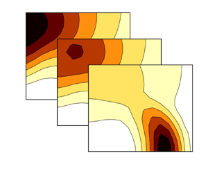
Figure 2 shows the accelerating laminar profiles at $Re=\{10,500\}$ and $\kappa =\{0.01,0.1\}$. Similarly, figure 3 shows the deceleration laminar profiles for the same parameters. At low Reynolds numbers $Re$ and low values of $\kappa$ the flow closely resembles simple shear at different shear rates (i.e. $U=g_w(t)y$), whereas with increased $Re$ and $\kappa$ the profiles become more curved. This curvature stems from a delay in the transfer of momentum from the wall to the middle of the channel. At higher $Re$ this transfer is slower and at higher $\kappa$ the rate of change of velocity at the wall increases. At the largest values of $Re$ and $\kappa$ the difference between acceleration and deceleration is exemplified. In this case, we observe that the accelerating profile maintains a positive gradient throughout the domain, while the decelerating profile shows a negative gradient near the wall. In § 3 we investigate the influence of these profiles on the stability of the flow.

Figure 2.

Laminar accelerating WDF. The Reynolds number and acceleration parameter for each flow are noted in the figure. The solution is shown at times $t=[0,2,5,10,20,40,60,80,100]$.

Figure 3.

Laminar decelerating WDF. The Reynolds number and deceleration parameter for each flow are noted in the figure. The solution is shown at times $t=[0,2,5,10,20,40,60,80,100]$.

2.2. Pressure-driven flow

We follow a similar approach to find the laminar flow solution for time-varying pressure gradients. In the case of PDF, we expect the solution to be even $U(y,t)=U(-y,t)$. In Cartesian coordinates, this suggests a solution of the heat equation using a cosine basis. We thus seek solutions of the form

(2.17)\begin{equation} U(y,t)=f_p(y,t)+ \frac{Re}{2} g_p(t)(y^2-1) + g_e(t). \end{equation}

Inserting this expression into (2.2)–(2.4) results in an equation for $f_p$ of the form

(2.18)\begin{equation} \frac{\partial f_p}{ \partial t}+\frac{Re}{2}\frac{{\rm d} g_p}{{\rm d} t}(y^2-1)+\frac{{\rm d} g_e}{{\rm d} t}=\frac{1}{Re}\frac{\partial^2 f_p}{\partial y^2}, \end{equation}

with boundary conditions

(2.19)\begin{equation} f_p(y={\pm} 1,t)=0 \end{equation}

and initial condition

(2.20)\begin{equation} f_p(y,0)=h_e-\frac{Re}{2}g_p(0)(y^2-1)-g_e(0). \end{equation}

To solve (2.18), we represent $f_p$ as

(2.21)\begin{equation} f_p(y,t)=\sum_{n=0}^\infty \hat{f}_{p,n}(t)\cos\left[\left(n+\frac{1}{2}\right){\rm \pi} y\right]. \end{equation}

The boundary conditions associated with all terms in (2.18) and (2.20) are satisfied by our cosine basis. To solve for the coefficients $\hat {f}_{p,n}(t)$, we repeat the procedure used for WDF. First, we combine (2.21) with (2.18) and take the inner product of the result with $\cos ((m+1/2){\rm \pi} y)$ leading to

(2.22)\begin{equation} \frac{{\rm d} \hat{f}_{p,m}}{{\rm d} t}=\frac{16 Re ({-}1)^m}{(2 {\rm \pi}m+{\rm \pi})^3}\frac{{\rm d} g_p}{{\rm d} t}- \frac{4 ({-}1)^m}{2 {\rm \pi}m+{\rm \pi}} \frac{{\rm d} g_e}{{\rm d} t}-b_m\hat{f}_{p,m}, \end{equation}

with $b_m=(2 {\rm \pi}m+{\rm \pi} )^2/(4Re)$. Solving (2.22) produces

(2.23)\begin{align}\hat{f}_{p,m}= {\rm e}^{{-}b_mt} \left[\frac{16 Re ({-}1)^m}{(2 {\rm \pi}m+{\rm \pi})^3} \int_0^t {\rm e}^{b_mt'}\left.\frac{{\rm d} g_p}{{\rm d} t}\right|_{t=t'} {\rm d} t'-\frac{4 ({-}1)^m}{2 {\rm \pi}m+{\rm \pi}} \int_0^t {\rm e}^{b_mt'}\left.\frac{{\rm d} g_e}{{\rm d} t}\right|_{t=t'} {\rm d} t' +C_{2,m} \right]. \end{align}

Then, to solve for the constant $C_{2,m}$, we take the inner product of the initial condition ((2.20)) with $\cos ((m+1/2){\rm \pi} y)$ to obtain

(2.24)\begin{equation} C_{2,m}=\int_{{-}1}^1\left[h_e-\frac{Re}{2}g_p(0)(y^2-1)-g_e(0)\right] \cos\left[\left(m+\frac{1}{2}\right){\rm \pi} y\right] {{\rm d} y}. \end{equation}

If the initial profile is parabolic and there is no wall motion, then $C_2$=0. Finally, by inserting $\hat {f}_{p,n}$ into (2.17), we find the laminar profile

(2.25)\begin{align} &U(y,t)\nonumber\\ &\quad =\sum_{n=0}^\infty {\rm e}^{{-}b_nt} \!\left[\frac{16 Re ({-}1)^n}{(2 {\rm \pi}n+{\rm \pi})^3} \int_0^t {\rm e}^{b_nt'}\left.\!\frac{{\rm d} g_p}{{\rm d} t}\right|_{t=t'} {\rm d} t'-\frac{4 ({-}1)^n}{2 {\rm \pi}n+{\rm \pi}} \int_0^t {\rm e}^{b_nt'}\left.\frac{{\rm d} g_e}{{\rm d} t}\right|_{t=t'\!} {\rm d} t' +C_{2,n} \!\right] \nonumber\\ &\qquad \cos\left[\left(n+\frac{1}{2}\right){\rm \pi} y\right]+\frac{Re}{2}g_p(t)(y^2-1) + g_e(t). \end{align}

In Appendix A we provide analytical expressions for the integral in (2.25) for representative flows (see table 1 in Appendix A) and we validate the solution against Womersley flow.

As with the WDF, we study the effect of acceleration and deceleration in the pressure-driven case (here we let $g_e(t)=0$). A natural first choice for examining the impact of acceleration and deceleration might be to set the pressure gradient to the same profiles used for the wall velocities (i.e. $g_p(t)=1-{\rm e}^{-\kappa t}$ and $g_p(t)={\rm e}^{-\kappa t}$). In the case of PDF, we non-dimensionalize the velocity by the maximum centreline velocity. However, the pressure gradient required to satisfy this non-dimensionalization is $g_p=-2/Re$ either at $t=0$ or as $t\rightarrow \infty$. This means that $g_p(t)=1-{\rm e}^{-\kappa t}$ and $g_p(t)={\rm e}^{-\kappa t}$ do not properly satisfy the correct profiles, and multiplying these quantities by $-2/Re$ would result in a different pressure gradient profile for different Reynolds numbers.

Instead of prescribing the same pressure gradient across all cases, we enforce an exponentially decaying accelerating or decelerating flow rate according to

(2.26)\begin{equation} Q(t)=\tfrac{2}{3}(1-{\rm e}^{-\kappa t}) \end{equation}

and

(2.27)\begin{equation} Q(t)=\tfrac{2}{3}({\rm e}^{-\kappa t}), \end{equation}

respectively. These flow rates correspond to a unit centreline streamwise velocity for a parabolic profile. Note that flow rate and mean velocity are synonymous here. As with wall motion, we delve into the details of this non-dimensionalization in § 2.3.

Prescribing a flow rate requires a corresponding pressure gradient to achieve this flow rate. We first show that accounting for all continuous flow rates requires pressure gradients that can undergo a step change at $t=0$, after which we compute the pressure gradients $g_p$ and use it to approximate $U$. We calculate the flow rate by integrating (2.25) in the wall-normal direction and dividing by twice the channel height to result in

(2.28)\begin{equation} Q(t)=\sum_{n=0}^\infty {\rm e}^{{-}b_nt} \left[ \frac{32 Re }{(2{\rm \pi} n+{\rm \pi})^4} \int_0^t {\rm e}^{b_nt'}\left.\frac{{\rm d} g_p}{{\rm d} t}\right|_{t=t'} {\rm d} t' +\frac{2 ({-}1)^n C_{2,n}}{2{\rm \pi} n+{\rm \pi}}\right] -\frac{Re}{3} g_p(t). \end{equation}

Evaluating (2.28) at $t=0$ and simplifying the resulting expression leads to

(2.29)\begin{equation} Q(0)=\sum_{n=0}^\infty \frac{2 ({-}1)^n}{2{\rm \pi} n+{\rm \pi}} \int_{{-}1}^1 h_e(y)\cos\left[\left(n+\frac{1}{2}\right){\rm \pi} y\right]{{\rm d} y}, \end{equation}

which shows that the initial flow rate only depends on the initial velocity profile, as expected. Taking the derivative of (2.28), we get after simplifications

(2.30)\begin{equation} \frac{{\rm d} Q}{{\rm d} t}={-}\sum_{n=0}^\infty \frac{8}{(2{\rm \pi} n+{\rm \pi})^2}\, {\rm e}^{{-}b_nt} \int_0^t {\rm e}^{b_nt'}\frac{{\rm d} g_p(t')}{{\rm d} t} \, {\rm d} t'. \end{equation}

From this expression, we note that a jump discontinuity is required for $g_p$ as $t\rightarrow 0$. If $g_p$ were a continuous function, (2.30) would indicate that $\lim _{t\rightarrow 0}\, {\rm d} Q/ {\rm d} t=0$. However, our desired flow rate results in $\lim _{t\rightarrow 0} \, {\rm d} Q/ {\rm d} t=\pm 2k/3$. Thus, satisfying this derivative constraint necessitates a step change in the pressure gradient at $t=0$ that can be formulated by

(2.31)\begin{equation} g_p(t)=H(t)\hat{g}_0+\hat{g}_p(t), \end{equation}

with $H(t)$ as the Heaviside function, $\hat {g}_0$ as a constant and $\hat {g}_p$ as a continuous temporal function. Furthermore, we may use ${\rm d} Q/ {\rm d} t$ to compute the constant $\hat {g}_0$ by taking the derivative of (2.31) and combining it with 2.30 to produce

(2.32)\begin{equation} \lim_{t \rightarrow 0} \frac{{\rm d} Q}{{\rm d} t}={-}\hat{g}_0. \end{equation}

The above expression indicates that only flow rates with $\lim _{t\rightarrow 0}\,{\rm d} Q/ {\rm d} t=0$ can be constructed with a continuous pressure gradient.

Now that we know the form that the pressure gradient must take, we can numerically solve for $g_p(t)$ to satisfy the flow rates given by (2.26) and (2.27). In short, we use the trapezoidal rule on all the integrals and then solve for $g_p(t)$. We include a detailed description of this procedure in Appendix D. In figure 4 we present examples of the numerically computed pressure gradients and the flow rates of the velocity profiles computed using these gradients at $Re=500$ and $\kappa =0.1$. Both pressure gradient profiles start with a constant pressure gradient for achieving zero flow (in the case of acceleration) or a parabolic profile (in the case of deceleration). At start-up, there is a step change in the pressure gradient that subsequently grows or decays toward the pressure gradient needed to maintain the long-time solution. The excellent match of the prescribed flow rates and the computed flow rates in figures 4(c) and 4(d) validate the computed pressure gradients.

Figure 4.

Plots (a) and (b) are the pressure gradient for flow rates of $Q_t=(2/3)(1-{\rm e}^{-\kappa t})$ and $Q_t=(2/3)\,{\rm e}^{-\kappa t}$ at $Re=500$ and $\kappa =0.1$ (the grey dashed line is the expected long-time value). Plots (c) and (d) are the flow rates $Q_p$ computed from applying the pressure gradients in (a) and (b).

In figure 5 we display the laminar flow solutions with the numerically computed pressure gradient for accelerating cases at $Re=\{10,500\}$ and 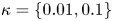$\kappa =\{0.01,0.1\}$; in figure 6 we show the laminar profiles for decelerating cases with the same parameters. For the accelerating cases, increasing $Re$ and $\kappa$ produces transient dynamics that are more plug like. For the decelerating cases, the gradient is diminished near the wall compared with the accelerating cases, and at sufficiently high $Re$ and $\kappa$, the profile exhibits backflow to maintain the appropriate flow rate. Similar to the decelerating WDF, we show in § 3 that this profile leads to destabilization.

Figure 5.

Laminar accelerating PDF. The Reynolds number and acceleration parameter for each flow are denoted in the figure. The solution is shown at times $t=[0,2,5,10,20,40,60,80,100]$.

Figure 6.

Laminar decelerating PDF. The Reynolds number and deceleration parameter for each flow are denoted in the figure. The solution is shown at times $t=[0,2,5,10,20,40,60,80,100]$.

Finally, we emphasize that the solutions provided in (2.14) and (2.25) are applicable for odd and even functions, respectively. Owing to linear superposition, any function may be represented by simply adding the two solutions together. Thus, the solutions presented in §§ 2.1 and 2.2 are valid for arbitrary streamwise wall motion and pressure gradients and can accommodate arbitrary wall-normal varying initial conditions.

2.3. Comments on non-dimensionalization

Before investigating the stability of these flows, we discuss the non-dimensionalization of the problem set-up. Thus far, the equations presented do not depend on the characteristic velocity $U_b$. The choice of $U_b$ depends on the selection of the boundary conditions, or pressure gradient, and should be selected to eliminate one of the dimensional parameters driving the flow. To illustrate this point, let us consider the case of accelerating and decelerating wall motion. In dimensional form we may write the velocity at the wall as

(2.33)\begin{equation} g^*_w(t)=u^*_i\,{\rm e}^{-\kappa^*t^*}+u^*_f(1-{\rm e}^{-\kappa^*t^*}), \end{equation}

which, after non-dimensionalization, becomes

(2.34)\begin{equation} g_w(t)=u_i\,{\rm e}^{-\kappa t}+u_f(1-{\rm e}^{-\kappa t}), \end{equation}

with non-dimensional scaling of $u_i=u^*_i/U_b$, $u_f=u^*_f/U_b$ and $\kappa =\kappa ^*h/U_b$. As such, the most natural choice for non-dimensionalization is to select a characteristic velocity that forces $u_i=1$, $u_f=1$ or $\kappa =1$. We consider flows that start from rest ($u_i=0$) or end at rest ($u_f=0$), so we choose the other velocity as our characteristic velocity $U_b$ and vary the non-dimensional exponential decay parameter $\kappa$. Notably, this decay parameter is inversely proportional to the characteristic time scale, for example, the half-life $t_{1/2}=\ln (2)/\kappa$. This suggests that, as we vary $Re$ and $\kappa$, we vary two time scales: the time scale over which the fluid in the middle of the channel reacts to wall motion due to viscosity and the time scale over which the wall motion reaches the final velocity. While it may also be possible to consider the viscous time scale, we adopt the advective scale due to the fast motion imposed during the acceleration and deceleration process. The laminar flow depends on both non-dimensional parameters $Re$ and $\kappa$, so we must vary both when investigating stability.

In contrast to the WDF, the selection of the characteristic velocity in the pressure-driven case is less obvious. The pressure gradient drives a flow with a characteristic velocity, but it is difficult to determine this characteristic velocity before prescribing the pressure gradient. To address this issue, we instead use the flow rate to determine the characteristic velocity. Additionally, by prescribing an accelerating or decelerating flow rate, we are directly accelerating or decelerating the mean velocity, whereas accelerating or decelerating the pressure gradient has an unclear effect on the mean velocity.

As with wall motion, we non-dimensionalize around either the long-time or the initial profile, which in the case of the accelerating or decelerating profile corresponds to a parabolic profile. This results in the dimensional flow rate equation

(2.35)\begin{equation} Q^*=\frac{1}{2h}\int_{{-}h}^h\frac{U(y=0)}{h^2}(h^2-y^{*2})\,{{\rm d} y}^*. \end{equation}

After evaluating the integral and using the non-dimensionalization of $Q=Q^*/U_b$, (2.35) simplifies to

(2.36)\begin{equation} Q=\frac{2U(y=0)}{3U_b}. \end{equation}

We may then set the characteristic velocity as either the final or initial centreline velocity ($U(y=0)=U_b$), which is satisfied when the flow rate is $Q=2/3$. Thus, we satisfy this non-dimensionalization for the exponentially decaying acceleration and deceleration cases when either $Q_\infty$ or $Q_0$ equal 2/3 in $Q(t)=Q_\infty (1-{\rm e}^{-\kappa t})+Q_0\,{\rm e}^{-\kappa t}$. As we investigate accelerating from rest and decelerating to rest in this work, we only need to sweep over the non-dimensional exponential decay parameter $\kappa$.

3.1. Maximum linear amplification

Non-normal linear operators can support large levels of transient growth, even though the operator's eigenvalues indicate asymptotic stability (all eigenvalues have negative real parts). We hence investigate this transient behaviour by computing the maximum possible amplification of initial energy density

(3.19)\begin{equation} G(t;\alpha,\beta,t_0,Re,\kappa)=\max_{\boldsymbol{q}(t_0)\neq 0} \frac{\|\boldsymbol{q}(t)\|^2_E}{\|\boldsymbol{q}(t_0)\|^2_E}= \max_{\boldsymbol{q}(t_0)\neq 0} \frac{\|{\boldsymbol{\mathsf{A}}}(t)\boldsymbol{q}(t_0)\|^2_E}{\|\boldsymbol{q}(t_0)\|^2_E}, \end{equation}

where $\|\cdot \|_E$ is the energy norm, the details of which we address below. We refer to the quantity $G(t)$ as amplification or growth. In the above expression, we emphasize that this amplification depends upon the wavenumbers of the perturbation, $\alpha$ and $\beta$, the time horizon $[t_0, t]$ over which the perturbation is observed and the parameters of the base flow $Re$ and $\kappa$. For brevity, we omit this explicit parameter dependence in what follows. The transient amplification is taken as the maximum relative increase (or gain) in perturbation energy that can be experienced by any initial perturbation $\boldsymbol {q}(t_0)$ over a given time frame $[t_0,t].$ Notably, a temporal series of $G(t)$ need not arise from the same perturbation $\boldsymbol {q}(t_0)$, but stem from a range of initial perturbations. Consequently, the curve $G(t)$ can be thought of as an envelope bounding the energy amplification of all initial conditions.

A common approach to solving for $G(t)$ is based on the adjoint method (Andersson, Berggren & Henningson Reference Andersson, Berggren and Henningson1999). However, when the matrix describing the linearized equations of motion is rather small, it becomes computationally tractable to compute ${\boldsymbol{\mathsf{A}}}(t)$ directly. With ${\boldsymbol{\mathsf{A}}}(t)$ explicitly available, we can capitalize on the fact that (3.19) closely resembles the spectral norm of ${\boldsymbol{\mathsf{A}}}(t)$, which only requires a singular value decomposition. However, as noted above, the energy norm, not the $L_2$ norm is used in (3.19). For this reason, we must recast this problem as an equivalent $L_2$-norm problem to proceed.

We define the energy norm according to

(3.20)\begin{equation} \|\boldsymbol{q}\|_E^2=\int_{{-}1}^1 (|D\hat{v}|^2+k^2|\hat{v}|^2+|\hat{\omega}_y|^2)\,{{\rm d} y}. \end{equation}

As shown in Gustavsson (Reference Gustavsson1986), dividing this quantity by $2k^2$ and integrating over all wavenumbers produces the kinetic energy of $\boldsymbol {u}'$. As we consider the relative energy amplification for perturbations at a specific set of wavenumbers, this normalization and integration approach is not necessary for the computation of the growth $G(t)$ (i.e. the normalization constant cancels out in (3.19)). In Appendix B we show how this energy norm can be recast into an equivalent $L_2$ norm by defining a matrix $\boldsymbol {V}$ such that $\|\boldsymbol {q}\|^2_E=\|\boldsymbol {V}\boldsymbol {q}\|^2$. We then compute the maximum amplification as

(3.21)\begin{equation} G(t)=\max_{\boldsymbol{q}(t_0)\neq 0} \frac{\|\boldsymbol{V}{\boldsymbol{\mathsf{A}}}(t)\boldsymbol{q}(t_0) \|^2}{\|\boldsymbol{V}\boldsymbol{q}(t_0)\|^2}=\max_{\boldsymbol{x}(t_0)\neq 0} \frac{\|\boldsymbol{V}{\boldsymbol{\mathsf{A}}}(t)\boldsymbol{V}^{{-}1} \boldsymbol{x}(t_0)\|^2}{\|\boldsymbol{x}(t_0)\|^2}= \|\boldsymbol{V}{\boldsymbol{\mathsf{A}}}(t)\boldsymbol{V}^{{-}1}\|^2, \end{equation}

where $\boldsymbol {x}=\boldsymbol {V}\boldsymbol {q}$ and the spectral norm of the matrix corresponds to the largest singular value.

In what follows, we compute $G(t)$ by approximating $\boldsymbol {V}$ and ${\boldsymbol{\mathsf{A}}}(t)$ on a grid of $M=64$ Chebyshev collocation points using a time step of $\Delta t=0.01$ for both WDF and PDF. We again approximate the base flow with $100$ basis functions as in § 2. To illustrate how the amplification varies over time, we consider accelerating and decelerating WDF and PDF at $Re=500$ and $\kappa =0.1$ in figures 7 and 8. Note that these laminar profiles were shown in figures 2, 3, 5 and 6.

Figure 7.

Amplification $G(t)$ for perturbations applied at different times $t_0$ to accelerating (‘Acc’), decelerating (‘Dec’) and constant WDF at $Re=500$ and $\kappa =0.1$. Amplification shown for (a) $[\alpha,\beta ]=[1.2,0]$ and (b) 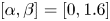$[\alpha,\beta ]=[0,1.6]$. Perturbations at times $t_0=[0,10,20,40,60,80,100]$ are shown.

Figure 8.

Amplification $G(t)$ for perturbations applied at different times $t_0$ to accelerating (‘Acc’), decelerating (‘Dec’) and constant PDF at $Re=500$ and $\kappa =0.1$. Amplification shown for (a) $[\alpha,\beta ]=[2,0]$ and (b) $[\alpha,\beta ]=[0,1.8]$. Perturbations at times $t_0=[0,10,20,40,60,80,100]$ are visualized.

In figure 7 we plot the amplification $G(t)$ with different parameters for constant, accelerating and decelerating WDF considering strictly streamwise perturbations (figure 7a) and strictly spanwise perturbations (figure 7b). Most notably, streamwise perturbations subjected to the decelerating base flow result in orders of magnitude larger growth than any perturbation of the constant or accelerating flows, both of which only show small growth at early times. Additionally, the largest amplification in the decelerating cases comes from perturbing the flow at early times, but not at $t_0=0$. In contrast, the accelerating case exhibits the largest growth for perturbations at later times, when the flow behaves more like a steady flow with a constant profile.

When only spanwise perturbations are considered (figure 7b) the constant profile exhibits the largest amplification of all cases. The accelerating and decelerating cases gradually transition between the amplification of the constant profile and the amplification in the case of no flow, as the time of the initial perturbation $t_0$ varies. Naturally, the accelerating case transitions from lower amplification to higher amplification, and the decelerating case transitions from higher amplification to lower amplification, as $t_0$ increases. This suggests that the shapes of the accelerating and decelerating base flows are less important to the growth of spanwise perturbations.

In figure 8 we show the maximum amplification for constant, accelerating and decelerating PDF. Once again figure 8(a) illustrates that streamwise perturbations about the decelerating base flow exhibit orders of magnitude larger amplification than the other cases, and streamwise perturbations in the constant and accelerating flows experience little growth. In figure 8(b) we again see that spanwise perturbations exhibit the largest amplification for the constant profile, and the accelerating and decelerating cases gradually move between the constant profile and the case of no flow.

Both results for WDF and PDF indicate that perturbations about decelerating laminar base flows may exhibit orders of magnitude greater amplification than perturbations about accelerating or constant laminar profiles. This amplification about decelerating flows occurs predominantly for perturbations with streamwise variations. In contrast, spanwise perturbations lead to the largest energy amplification in constant and accelerating flows.

3.2. Maximum growth for accelerating and decelerating flows

In the previous section we computed $G(t)$ at specific values of $Re, \alpha, \beta$ and $\kappa$. Here, we perform a detailed examination of the maximum growth when sweeping over these parameters for perturbations to the laminar flows at the beginning of the acceleration or deceleration phase at $t_0=0$. Although perturbations at later $t_0$ can exhibit larger growth, the mechanisms of growth at $t_0=0$ and at the optimal $t_0$ tend to be similar in this work. In § 3.5 we further investigate the effect of optimizing over $t_0$ to illustrate this point. In figure 9 we present the maximum growth $G_{max}=\max _{\alpha,\beta,t} G(t)$ over a set of $Re$ and $\kappa$ for accelerating and decelerating WDF and PDF. As a point of reference, we normalize the growth by the maximum value $G_0$ obtained from the constant WDF or PDF case. Both accelerating WDF and PDF exhibit less growth than the constant laminar flow. The growth relative to the constant laminar profile is lowest at the lowest value of $\kappa$ and moderately low Reynolds number $Re$. As $\kappa$ and $Re$ increase, the growth appears to level out at around a tenth of the constant flow.

Figure 9.

Maximum growth normalized by the maximum growth of perturbations in the constant flow varied over different $Re$ and $\kappa$: (a) for accelerating WDF, (b) for decelerating WDF, (c) for accelerating PDF and (d) for decelerating PDF.

In contrast to the accelerating laminar cases, the decelerating laminar cases exhibit far larger amplification of perturbations than the constant laminar case. For WDF at $Re=800$, we see $10^4$ times larger amplification over the constant profile. Upon further increasing $\kappa$ and $Re$, the relative amplification continues to grow. Decelerating PDF also exhibits this large amplification at high $Re$ and $\kappa$.

The two competing factors are the rate $\kappa$ at which the walls move and the rate at which the flow can react to this motion, i.e. $1/Re$. At large values of $\kappa$, the wall motion is fast and the laminar profile is sensitive to changes in $Re$ while insensitive to changes in $\kappa$. At the other extreme of small $\kappa$, the laminar flows change so slowly that the growth of perturbations behaves similarly to the growth of perturbations in the constant laminar case or the no-flow case.

We focus on this range of $Re$ and $\kappa$ values because these values show where a transition in growth is exhibited in the decelerating cases. As $\kappa$ continues to increase, the results converge toward impulsive wall motion (i.e. Stokes’ first problem). Similarly, if we continue to increase the Reynolds number, we will find that, at moderate $\kappa$ values, there is a consistent scaling in the maximum amplification as the Reynolds number changes. Figure 10 shows how $G_{max}$ varies with $Re$ at $\kappa =0.1$ for constant, accelerating and decelerating WDF and PDF. We also show the $Re^2$ scaling discussed in Reddy & Henningson (Reference Reddy and Henningson1993) as ‘Const Fit’ (using the same values) and the best exponential fit for the decelerating cases at $Re>400\vphantom{10^{\frac{1}{2}}}$ as ‘Dec Fit’ ($G_{max}=0.0015\times 10^{0.012Re}$ for WDF and $G_{max}=0.0199\times 10^{0.009Re}$ for PDF). Both the constant and accelerating cases exhibit similar trends over all Reynolds numbers $Re$, while the decelerating case exhibits two distinct behaviours. At low $Re$, the decelerating case shows the same $Re^2$ scaling as the constant case, and at high $Re$ the decelerating case shows a $10^{Re}$ scaling. As mentioned in § 1, this behaviour was also observed in oscillatory flows shown in Xu et al. (Reference Xu, Song and Avila2021). However, the optimal perturbations in their work did not exhibit a shift wavenumber as $Re$ increased, which, as we will show, is not the case for these decelerating flows. For low values of $Re,$ viscous forces quickly modify the flow in response to the wall velocity, and the growth behaves similarly to a constant flow. When the Reynolds number is high, the flow reacts more slowly to the wall motion, allowing the laminar base flow to exhibit high curvature, leading to the $10^{Re}$ scaling. However, unlike the decelerating case, the accelerating case only exhibits the $Re^2$ scaling. Thus, we must further examine the shape of the perturbations to explain this difference in scaling.

Figure 10.

Plots of $G_{max}$ as a function of $Re$ for accelerating flow (‘Acc’), decelerating flow (‘Dec’) and constant flow (‘Const’) at fixed $\kappa =0.1$ for (a) WDF and (b) PDF. The fitting lines are described in the text.

To better understand the cause for decreased amplification in the accelerating case and increased amplification in the decelerating case, we consider the wavenumbers at which the amplification occurs. Figure 11 shows the maximum amplification $\max _tG(t)$ at multiple values of $Re$, $\kappa$, $\alpha$ and $\beta$ for accelerating WDF. Analogously, figure 12 shows the same results for decelerating WDF. Each figure is normalized by the maximum amplification over all wavenumbers, which is indicated near the top right corner of each plot.

Figure 11.

Maximum amplification of perturbations $\max _tG(t)$ for accelerating WDF at different wavenumbers and acceleration rates (denoted in the figure).

Figure 12.

Maximum amplification of perturbations $\max _tG(t)$ for decelerating WDF at different wavenumbers and deceleration rates (denoted in the figure).

For accelerating WDF, the most amplified perturbations are ones that vary in the spanwise direction at $[\alpha,\beta ]\approx [0,1.6]$. Likewise, the constant laminar profile exhibits maximal amplification for perturbations that vary in the spanwise direction at the same spanwise wavenumber (Reddy & Henningson Reference Reddy and Henningson1993). Referring back to (3.11), we see that for $\alpha =0$, $\mathscr {L}_{os}$ and $\mathscr {L}_{sq}$ no longer depend on the laminar base flow. Thus, the influence of the laminar profile only enters through the derivative of the laminar profile in the coupling term $\mathscr {L}_c$. This observation likely explains the weaker dependence on shape exhibited in the amplification shown in figures 7(b) and 8(b).

Perturbations in decelerating laminar flows exhibit a much different dependency on the wavenumbers as $Re$ and $\kappa$ vary. At a low rate of deceleration $\kappa$, the largest maximum amplification arises from spanwise perturbations. Upon increasing $\kappa,$ the largest maximum amplification moves towards perturbations with streamwise variations. A similar trend holds for the Reynolds number, such that for $Re=500$ and $\kappa =1$, the maximum amplification is due to a streamwise varying perturbation with wavenumbers $[\alpha,\beta ]\approx [1.2,0]$. Referring back to (3.11), we notice that, for $\beta =0$, the operator $\mathscr {L}_{c}$ vanishes, hence decoupling $\hat {v}$ and $\hat {\omega }_y$. Furthermore, spanwise wavenumbers cause $\mathscr {L}_{os}$ and $\mathscr {L}_{sq}$ to both depend on the laminar profile. This indicates that the high levels of amplification to perturbations in the decelerating profiles are directly due to the influence of the velocity and second derivative of the velocity for the decelerating laminar flow, and not due to the interactions between wall-normal velocity and vorticity, as is the case for accelerating and constant profiles.

Next, we investigate the wavenumbers that lead to the largest amplification for accelerating and decelerating PDFs. In figures 13 and 14, we show the maximum amplification for accelerating and decelerating PDFs, respectively. For accelerating flow, there is no growth, or very small growth, at low $\kappa$. As $\kappa$ and $Re$ increase, the maximum amplification increases, and the maximum amplification localizes to spanwise wavenumbers. The maximum amplification occurs at a streamwise wavenumber of $\beta \approx 1.8$, while the constant laminar flow exhibits maximum amplification at a wavenumber of $\beta \approx 2.04$ (Trefethen et al. Reference Trefethen, Trefethen, Reddy and Driscoll1993).

Figure 13.

Maximum amplification of perturbations $\max _tG(t)$ for accelerating PDF at different wavenumbers and acceleration rates (denoted in the figure).

Figure 14.

Maximum amplification of perturbations $\max _tG(t)$ for decelerating PDF at different wavenumbers and deceleration rates (denoted in the figure).

In the case of decelerating flow, we again see a gradual shift from spanwise dominant to streamwise dominant perturbations. At low values of $\kappa$ and $Re$, the maximum amplification is centred at $[\alpha,\beta ]\approx [0,2.1]$, similar to the constant profile. On the other extreme, i.e. high values of $\kappa$ and $Re$, the maximum amplification is centred on streamwise perturbations with a wavenumber of $[\alpha,\beta ] \approx [2.2,0]$. As $\kappa$ and $Re$ increase, the maximum amplification shifts between these two types of perturbations. Moreover, if the Reynolds number is too low, the maximum amplification will never drift towards streamwise perturbations, and at higher values of $Re,$ the range of $\kappa$ over which this transition occurs becomes much smaller. This transition is reflected in figure 9 where the maximum growth is plotted vs $Re$ and $\kappa.$

3.3. Structure of optimal perturbations

In the previous sections we explored how the accelerating laminar flow displays maximum amplification for spanwise perturbations, while the decelerating laminar flow shows maximum amplification for streamwise perturbations. These results indicate the shape of the maximally amplified perturbation in the periodic ccordinate directions, but not in the wall-normal direction. In this section we investigate the structure of the specific perturbations that develop to $\max _t G(t)$. We first outline the calculation of the optimal perturbation and then follow the amplification of that perturbation through time, along with its spatial profile.

For calculating the optimal perturbation, recall that the amplification at some time $t'$ is the energy gain of a perturbation that leads to the largest energy growth over all unit-norm initial perturbations $\boldsymbol {q}_0$. We compute this quantity by performing the singular value decomposition

(3.22)\begin{equation} \boldsymbol{V}{\boldsymbol{\mathsf{A}}}(t')\boldsymbol{V}^{{-}1}={\boldsymbol{\mathsf{U}}}_S\varSigma {\boldsymbol{\mathsf{V}}}_S^T, \end{equation}

where ${\boldsymbol{\mathsf{U}}}_S$ contains the left singular vectors, ${\boldsymbol{\mathsf{V}}}_S$ contains the right singular vectors and $\varSigma$ contains the singular values, ordered by size $\sigma _1\geq \sigma _2 \geq \cdots \geq \sigma _N,$ along its diagonal. The maximum amplification is then given by $\sigma _1^2$, and if we consider only the growth along this leading direction we obtain

(3.23)\begin{equation} \boldsymbol{V}{\boldsymbol{\mathsf{A}}}(t')\boldsymbol{V}^{{-}1}\boldsymbol{v}_{S,1}=\sigma_1 \boldsymbol{u}_{S,1}, \end{equation}

where $\boldsymbol {u}_{S,1}$ and $\boldsymbol {v}_{S,1}$ are the principal left and right singular vectors, respectively. The right singular vector $\boldsymbol {v}_{S,1}$ is transformed via the mapping $\boldsymbol {V}{\boldsymbol{\mathsf{A}}}(t')\boldsymbol {V}^{-1}$ onto $\boldsymbol {u}_{S,1}$ and stretched by a factor of $\sigma _1$. Owing to this relationship, we conclude that the initial perturbation leading to the maximum amplification at some time $t'$ is given by $\boldsymbol {v}_{S,1}$. We can subsequently evolve this perturbation in time according to the linearized equations of motion

(3.24)\begin{equation} \boldsymbol{v}(t)=\boldsymbol{V}{\boldsymbol{\mathsf{A}}}(t) \boldsymbol{V}^{{-}1}\boldsymbol{v}_{S,1}, \end{equation}

and, given $\Vert\boldsymbol {v}_{S,1}\Vert^{2}=1$, we can evaluate the perturbation energy as $G_p(t)=\|\boldsymbol {v}(t)\|^2$. In what follows, we compute the perturbation $\boldsymbol {v}_{S,1}$ from time $t'$ at which $G(t)$ is maximized ($t'=\text {argmax}_t G(t)$). We then display the evolution of the energy and the profile of $\boldsymbol {v}(t)$ through time. It is important to realize that the amplification that maximizes $G(t')$ at some time $t'$ need not necessarily maximize $G(t)$ for any other time.

3.3.1. Optimal perturbations in WDFs

First, we consider the accelerating and decelerating WDF cases. In figure 15(a) we show the energy of the optimal perturbation over time for accelerating WDF at $Re=500$ and $\kappa =0.1$. For this flow, we compute the optimal perturbation that reaches the maximum amplification at $t'=118$. At short times, the energy of the optimal perturbation falls below the envelope of $G(t)$, and at long times the energy of the optimal perturbation matches $G(t)$. This indicates that other perturbations lead to larger growth at shorter times, but the energy of these perturbations will not reach the long-time energy achieved by the optimal perturbation. In figure 15(b) we show the evolution of the perturbation at the times indicated in figure 15(a). We visualize the perturbation with contours of the streamfunction. The perturbation takes the form of streamwise vortices that initially decay in magnitude, but subsequently grow as the flow accelerates towards the simple shear profile. The shape of this perturbation closely resembles that of the optimal perturbation in constant WDF and grows via a ‘vortex-tilting’ mechanism (Butler & Farrell Reference Butler and Farrell1992). Unlike constant WDF, the perturbation in the accelerating flow exhibits an initial drop in energy due to the transient period in which the accelerating profile develops towards the simple shear profile.

Figure 15.

(a) Energy of the optimal perturbation and the envelope of growth for accelerating WDF ($Re=500$, $\kappa =0.1$). (b) Streamfunction of the perturbation as it evolves in time.

The dynamics of the perturbation in the decelerating case behave much differently from the constant WDF. Figure 16(a) shows the energy of the optimal perturbation for decelerating WDF and the largest real part of the eigenvalue of the time-varying linear operator $\lambda _{max}$ at $Re=500$ and $\kappa =0.1$. In this case, we compute the optimal perturbation that reaches its maximum amplitude at $t'=132$. Similar to the accelerating case, the energy of the perturbation falls below $G(t)$ at early times but matches $G(t)$ at long times. Unlike the accelerating case, the perturbation in the decelerating case exhibits initial growth, followed by decay, before growing again to reach much larger energy values. Notably, the second peak in the growth begins when the instantaneous eigenvalue becomes positive and decays when the eigenvalue becomes negative.

Figure 16.

(a) Energy of the optimal perturbation, the envelope of growth and the instantaneous eigenvalue for decelerating WDF ($Re=500$, $\kappa =0.1$). (b) Thin lines are the streamfunction of the perturbation as it evolves in time. The filled contour plot visualizes the production ((3.25)) normalized by the maximum absolute value (red indicates positive values and blue indicates negative values). The thick black line is the reference laminar profile ($U$), with a dot at the inflection point.

Along with the energy of the optimal perturbation, in figure 16(b) we show the evolution of the optimal perturbation for decelerating WDF. We also plot the laminar profile and the spatial energy production

(3.25)\begin{equation} P={-}u'v'\frac{\partial U}{\partial y}, \end{equation}

to identify the cause of energy growth. Note that this term lies in the production term of the energy equation (Serrin Reference Serrin1959; Conrad & Criminale Reference Conrad and Criminale1965)

(3.26)\begin{equation} \frac{{\rm d} E}{{\rm d} t}=\frac{{\rm d} }{{\rm d} t}\int_V \frac{\boldsymbol{u}'\boldsymbol{\cdot}\boldsymbol{u}'}{2}\, {\rm d} V={-}\int_V \frac{1}{Re} \nabla^2 \boldsymbol{u}' : \nabla^2 \boldsymbol{u}'\, {\rm d} V-\int_V \boldsymbol{u}'\boldsymbol{\cdot}\boldsymbol{\nabla} \boldsymbol{U} \boldsymbol{\cdot} \boldsymbol{u}'\, {\rm d} V. \end{equation}

In the inviscid case, for a $y$-dependent streamwise baseflow, this equation simplifies to

(3.27)\begin{equation} \frac{{\rm d} E}{{\rm d} t}=\int_V -u'v'\frac{{\rm d} U}{{\rm d} y}\, {\rm d} V=\int_V \frac{\partial \psi}{\partial y}\frac{\partial \psi}{\partial x}\frac{{\rm d} U}{{\rm d} y}\, {\rm d} V=\int_V - \left. \frac{{\rm d} y}{{\rm d} x}\right|_\psi \frac{{\rm d} U}{{\rm d} y}\, {\rm d} V, \end{equation}

where $\psi$ represents the streamfunction. Thus, energy increases when the term under the integral is negative or when the streamlines align opposite to the gradient of the laminar flow. This mechanism of growth is referred to as the Orr mechanism or the down-gradient Reynolds stress mechanism in Butler & Farrell (Reference Butler and Farrell1992).

At $t=0$ the streamfunction of the initial perturbation opposes the laminar shear, causing the initial gain in energy. The streamlines are advected by the laminar profile causing them to rotate and break up at $t=2$ and $t=5$. Over this time window, the energy grows. Then, at $t=10$ the streamlines become vertical and eventually align with the laminar shear at $t=15$ causing the energy to decrease. Finally, the streamlines once again advect and align opposite to the laminar shear, over much of the domain, causing the energy to increase. After $t\approx 50$, there is little change in the shape of the perturbation, which we show at $t=70$.

Throughout this time series, the energy production follows the anti-aligned streamlines supporting the claim that the Orr mechanism is responsible for this energy growth. In Morón, Feldmann & Avila (Reference Morón, Feldmann and Avila2022) the production was also shown to coincide with the inflection point for pulsatile flows. For WDF, the inflection point always remains in the centre of the channel. At early times, the location of the inflection point does not match energy production, but, at later times, energy is produced at the inflection point. It remains unclear if the inflection point plays an important role in our understanding of the stability of this problem. One approach to further investigate the significance of the inflection point could be to use a master-slave model that eliminates this inflection point, as was performed in Morón & Avila (Reference Morón and Avila2024).

Next, we show why this Orr mechanism leads to minimal growth in accelerating and constant WDFs. figure 17 shows the energy and evolution of the optimal perturbation for constant WDF at the same wavenumbers as in the decelerating case and for $t'=7.25$. The perturbation in constant WDF reaches a similar amplification to the first peak in the decelerating case, but then rapidly dies off. Figure 17(b) shows the evolution of this perturbation. The initial perturbation closely resembles the perturbation in the decelerating case, and it follows a similar evolution up to $t=7$ wherein the streamlines initially oppose the laminar shear before aligning vertically. However, in contrast to the decelerating case, the constant laminar profile rotates the streamlines and retains this alignment with the laminar shear causing the energy of the perturbation to drop drastically, as shown at $t=10$ and $t=13$.

Figure 17.

(a) Energy of the optimal perturbation and the envelope of growth for constant WDF ($Re=500$). (b) Thin lines are the streamfunction of the perturbation as it evolves in time. The filled contour plot visualizes the production ((3.25)) normalized by the maximum absolute value (red is positive and blue is negative).

We emphasize the key difference in the evolution of the decelerating flow and the accelerating or constant flow is this long-time alignment of the streamfunction. Streamwise perturbations in decelerating flows exhibit large growth because the streamfunction aligns opposite to the laminar shear. Streamwise perturbations in accelerating or constant flows exhibit small growth because the streamfunction aligns with the laminar shear. Thus, a key conclusion of our results is that there is a range of critical Reynolds numbers and deceleration rates where the optimal perturbations switch from spanwise to streamwise perturbations for decelerating flows. This transition occurs when growth due to vortex tilting is outpaced by growth due to the Orr mechanism. Once the Orr mechanism dominates, the maximum amplification scales exponentially with the Reynolds number resulting in massive amplification not experienced in accelerating or constant flows.

3.3.2. Optimal perturbations in PDFs

Next, we turn toward the accelerating and decelerating PDF cases. Figure 18(a) shows the energy of the optimal perturbation for accelerating PDF at $Re=500$ and $\kappa =0.1$. Here, the optimal perturbation reaches the maximum amplitude at $t'=78$. Qualitatively, an accelerating PDF shows the same characteristics as an accelerating WDF. The energy of the perturbation initially drops and then increases as the flow accelerates, and the perturbations again take the form of streamwise vortices. Figure 18(b) shows the evolution of the perturbation at the times indicated in figure 18(a). Again, the shape of this perturbation comes in the form of streamwise vortices, which agrees with the constant PDF case in Butler & Farrell (Reference Butler and Farrell1992).

Figure 18.

(a) Energy of the optimal perturbation and the envelope of growth for accelerating PDF ($Re=500$, $\kappa =0.1$). (b) Streamfunction of the perturbation as it evolves in time.

Lastly, we consider the case of decelerating PDF. In figure 19(a) we show the energy of the optimal perturbation that maximizes $G(t')$ at $t'=61$. Unlike the previous cases, even at short times the energy of the perturbation closely follows the envelope over all perturbations $G(t)$. The decelerating PDF does not exhibit a drop in energy, as seen in the decelerating WDF, because $\lambda _{max}$ becomes positive sooner. figure 19(b) shows the evolution of the optimal perturbation corresponding to the points in figure 19(a). Again, we show the laminar profile for reference. Similar to the decelerating WDF case, the initial profile opposes the laminar shear leading to growth. As this perturbation evolves, it is advected downstream and the streamfunction orients vertically, which momentarily damps growth. Then, the perturbation again aligns opposite to the laminar shear and stops moving as the base profile tends towards no flow. For constant PDF, the streamwise perturbations damp out rapidly (Butler & Farrell Reference Butler and Farrell1992), but here the time-varying nature of the base flow allows the perturbation to align opposite to the flow and experience extended periods of growth. Again, we see that the energy is produced at the locations of anti-alignment with the laminar shear. Unlike the WDF case, this production tends to stay near the wall-normal location of the inflection points, similar to Morón et al. (Reference Morón, Feldmann and Avila2022).

Figure 19.

(a) Energy of the optimal perturbation, the envelope of growth and the instantaneous eigenvalue for decelerating PDF ($Re=500$, $\kappa =0.1$). (b) Thin lines are the streamfunction of the perturbation as it evolves in time. The filled contour plot visualizes the production ((3.25)) normalized by the maximum absolute value (red indicates positive, blue indicates negative values). The thick black line is the reference laminar profile ($U$), with a dot at the inflection point.

3.4. Nonlinear evolution of perturbations

Thus far, we have shown the evolution of perturbations through the linearized equations of motion. In this section we investigate the evolution of optimal perturbations in DNS and the role of these optimal perturbations when perturbing the flow with random noise. We perform DNS of decelerating WDF and PDF at $Re=500$ and $\kappa =0.1$ Our DNS uses a Fourier–Chebyshev pseudo-spectral code implemented in Python (Linot, Zeng & Graham Reference Linot, Zeng and Graham2023a,Reference Linot, Zeng and Grahamb), which is based on the Channelflow code developed by Gibson (Reference Gibson2012), Gibson et al. (Reference Gibson2021). We use the Spalart-Moser Runge–Kutta (SMRK2) scheme (Spalart, Moser & Rogers Reference Spalart, Moser and Rogers1991) to integrate solutions forward in time. This is a multistage scheme that treats the linear term implicitly and the nonlinear term explicitly. The SMRK2 scheme only requires one flow field at one instant in time, which we require to satisfy the decelerating boundary condition at every time step. In the case of PDF we directly impose the exponentially decaying flow rate, not the numerical estimate of the pressure gradient shown in figure 4. For more details on the implementation of the DNS, we refer the reader to Linot et al. (Reference Linot, Zeng and Graham2023b) and Gibson (Reference Gibson2012).

First, we validate the results of the DNS by showing that it maintains the analytical laminar profiles. Here, we perform simulations with a time step of $\Delta t=0.01$ on a grid size of $[N_x,N_y,N_z]=[2,81,2]$ and a domain of $[L_x,L_y,L_z]=[1,2,1]$ with no noise. As the laminar flow only varies in the wall-normal direction, the choice of $N_x=2$ and $N_z=2$ was chosen to speed up the computation. Using more grid points in these directions does not influence the results. Figure 20 compares the laminar solutions derived in § 2 to the DNS, showing that the DNS and the laminar solution are in excellent agreement.

Figure 20.

Analytical and DNS solutions for laminar (a) WDF and (b) PDF at $Re=500$ and $\kappa =0.1$.

Next, we consider the effect of applying the optimal perturbations to both of these flows. In both cases, the optimal perturbations are predominantly streamwise structures. Due to this two dimensionality, we perform the DNS on a grid of size $[N_x,N_y,N_z]=[32,81,2]$ and a domain size of $[L_x,L_y,L_z]=[2{\rm \pi} /\alpha _{opt},2,1]$ with a time step of $\Delta t=0.01$. Simulating on more grid points in the spanwise direction does not change the results, since the initial perturbation does not vary in this direction. We initialize both DNS with an initial condition $\boldsymbol {u}=\boldsymbol {U}+\boldsymbol {u}'$, where we reduce the magnitude of the optimal perturbations shown in figures 16(a) and 19(a), such that $\boldsymbol {u}'=10^{-3}\boldsymbol {u}_p'$. With this initialization the energy ratio of the perturbation is $\|\boldsymbol {u}'\|_E^2/\|\boldsymbol {U}\|_E^2= {O}(10^{-7})$ in both cases. Figure 21 displays, for WDF, the energy of the perturbation from the DNS, and the shape of the perturbation as it evolves in time. The energy in the DNS matches the linearized solution extremely well until $t\approx 125$, at which point the energy of the DNS starts to drop more rapidly. At $t=125$, the energy ratio of the perturbation is $\|\boldsymbol {u}'\|_E^2/\|\boldsymbol {U}\|_E^2\approx 0.11$ due to the reduced energy in the laminar profile and the growth of the perturbation. The sizeable portion of energy contribution from the perturbation suggests that the assumption of linearity at this point likely breaks down. In figure 21(b) we show the evolution of the perturbation through time. Until $t\approx 75$, we see excellent agreement between the optimal perturbation computed via the linearized equations and the DNS. As mentioned, after this time the relative size of the perturbation becomes sufficiently large, and nonlinear effects distort the field, as shown in the final snapshot at $t=125$.

Figure 21.

(a) Energy of the optimal perturbation for decelerating WDF ($Re=500$, $\kappa =0.1$) determined by the linearized equations of motion $G_p$ and by the DNS $G_{DNS}$. (b) Streamfunction of the perturbation as it evolves in time (black is from the linearized equations and red is from the DNS).

In figure 22 we show the optimal perturbation in a DNS of PDF. Again, the energy of the DNS agrees well with the energy of the solution in the linearized equations at early times and begins to deviate around $t=50$. At the peak of $t=60$, the energy ratio of the perturbation is $\|\boldsymbol {u}'\|_E^2/\|\boldsymbol {U}\|_E^2\approx 0.03$. Figure 22(b) shows the evolution of the perturbation through time. Here, the perturbation in the DNS remains similar to the evolution in the linearized equations, even when the energy starts to differ at $t=60$.

Figure 22.

(a) Energy of the optimal perturbation for decelerating PDF ($Re=500$, $\kappa =0.1$) determined by the linearized equations of motion $G_p$ and by the DNS $G_{DNS}$. (b) Streamfunction of the perturbation as it evolves in time (black indicates the linearized equations and red is from the DNS).

We have established that the optimal perturbation exhibits large growth even in a DNS. As a next step, we investigate the relevance of this growth in the presence of random perturbations. We perform DNS on a grid of size $[N_x,N_y,N_z]=[32,81,32]$ and a domain size of $[L_x,L_y,L_z]=[2{\rm \pi} /\alpha _{opt},2,2 {\rm \pi}/\beta _{opt}]$ with a time step of $\Delta t=0.01$. Here, we chose $\beta _{opt}$ as the strictly spanwise perturbation that causes the largest amplification for $\kappa =0.1$ and $Re=500$. This choice of domain size allows the largest growing spanwise and streamwise perturbations to grow simultaneously. We then perturb this flow with Gaussian noise at every grid point such that $\boldsymbol {u}'\sim \mathcal {N}(0,\varepsilon ^2)$, where $\varepsilon =10^{-7}$. Even though this noise is initially not incompressible, the DNS enforces incompressibility after the first time step.

In figure 23(a) we show the energy of the optimal perturbation, the randomly perturbed field and the projection of the random perturbation onto the optimal perturbation for WDF at $Re=500$ and $\kappa =0.1$. The random perturbation exhibits a decay in energy until $t\approx 50$, followed by a growth in energy that peaks when the energy of the optimal perturbation peaks. At early times, this energy decay occurs because most modes decay, despite the energy associated with the optimal perturbation growing. It is not until later in the evolution of this noise that the optimal perturbation can grow sufficiently large to increase the energy of the random perturbation. The projection of the random perturbation onto the optimal perturbation shows that despite the drop in energy of the overall perturbation, the part associated with the optimal perturbation exhibits the expected growth. The slight mismatch between the projection and the energy of the optimal perturbation is conjectured to come from interactions between the modes, as they do not remain orthogonal during their temporal evolution. We also show the evolution of the random perturbation in figure 23(b). The random perturbation differs substantially from the optimal perturbation at early times, but begins to tilt against the laminar shear at $t\approx 25$, before exhibiting close agreement with the optimal perturbation at $t\geq 45$. We compute the streamlines for the random perturbation assuming the flow is two dimensional at $z=0$. Choosing a different $z$ location would influence the field at early times, but the random field becomes a streamwise perturbation, like the optimal perturbation, at later times.

Figure 23.

(a) Energy of the optimal perturbation for decelerating WDF ($Re=500$, $\kappa =0.1$) determined by the linearized equations of motion $G_p$ and energy of a random perturbation in a DNS $G_{DNS}$, along with the energy of the random perturbation projected onto the optimal perturbation $G_{Proj}$. (b) Streamfunction of the perturbation as it evolves in time (black is from the linearized equations and red is from the DNS).

Figure 24 shows the same results for PDF at $Re=500$ and $\kappa =0.1$. The energy of the random perturbation decreases until $t\approx 16$ before increasing and peaking at the same time as the optimal perturbation. Due to the faster time scale over which growth happens in this case, the projection of the random perturbation onto the optimal perturbation matches the energy of the optimal perturbation even at early times. Furthermore, the streamlines of the random perturbation agree with those of the optimal perturbation at $t\geq 25$. These figures show that, despite exhibiting far less growth, the random perturbation evolves into the optimal perturbation.

Figure 24.

(a) Energy of the optimal perturbation for decelerating PDF ($Re=500$, $\kappa =0.1$) determined by the linearized equations of motion $G_p$ and energy of a random perturbation in a DNS $G_{DNS}$, along with the energy of the random perturbation projected onto the optimal perturbation $G_{Proj}$. (b) Streamfunction of the perturbation as it evolves in time (black is from the linearized equations and red is from the DNS).

3.5. Optimal perturbation timing

Up to this point we have predominantly considered perturbations applied at the first instant of acceleration or deceleration. However, as noted in figures 7 and 8, perturbations can grow larger when applied at later times. In this section we investigate this behaviour by sweeping over the time $t_0$ when we apply the perturbation. Figure 25 shows the maximum amplification $G_{{max},t_0}=\max _{\alpha,\beta,t,t_0} G(t)$ and the time at which the perturbation is applied at various $Re$ and $\kappa$ for decelerating WDF and PDF. Similar to the results in figure 9, there is a massive increase in the amplification as $Re$ and $\kappa$ increase. For WDF, this increase in amplification now appears at lower values of both $Re$ and $\kappa$, in comparison to the $t_0=0$ case. Figures 25(c) and 25(d) show that this increase coincides with a substantial delay in the application of the perturbation. At low $\kappa$, this delay is largest, and decreases and converges as $\kappa$ increases. When $\kappa$ is small, the time scale associated with wall motion dominates; when $\kappa$ is large, the viscous time scale dominates.

Figure 25.

Panels (a) and (b) show the maximum growth normalized by the maximum growth of perturbations in the constant flow at various $Re$ and $\kappa$ for decelerating WDF and decelerating PDF. Panels (c) and (d) show the optimal perturbation timing at various $Re$ and $\kappa$ for decelerating WDF and decelerating PDF.

In figure 26 we show the optimal wavenumbers at which $G_{{max},t_0}$ is achieved. Qualitatively, these results agree with the results at $t_0=0$. At low $\kappa$ and $Re$, the optimal perturbations are spanwise with $\beta \approx 1.6$ for WDF and $\beta \approx 2.2$ for PDF. At high $Re$, the optimal perturbations are streamwise with $\alpha \approx 0.8$, at low $\kappa$, and $\alpha \approx 1.4$, at high $\kappa$, for WDF. In PDF the optimal perturbations are at $\alpha \approx 1.6$, at low $\kappa$, and $\alpha \approx 2.1$, at high $\kappa$. Again, this highlights that branch switching occurs at sufficiently high $Re$ and $\kappa$.

Figure 26.

Panels (a) and (b) show the optimal perturbation streamwise wavenumber at various $Re$ and $\kappa$ for decelerating WDF and decelerating PDF. Panels (c) and (d) show the optimal perturbation spanwise wavenumber at $Re$ and $\kappa$ for decelerating WDF and decelerating PDF.

Next, we investigate the shape of the optimal perturbations at the optimal timing and inform the results with linear stability analysis using the quasi-steady state approximation. Figure 27(a) shows the energy of the optimal perturbation, the real part of the largest instantaneous eigenvalue and the energy of evolving different eigenvectors forward in time for WDF at $Re=500$ and $\kappa =0.1$. Figure 27(b) shows the evolution of the optimal perturbation and the eigenvectors of the instantaneous linear operator at various times for WDF. This figure highlights three important times in the evolution of the optimal perturbation. First, the initial phase of the optimal perturbation occurs around when the maximum eigenvalue of the instantaneous linear operator becomes positive. Second, when the maximum eigenvalue peaks, the shape of the optimal perturbation and the instantaneous eigenvector closely resemble one another. Third, when the maximum eigenvalue drops below zero, the energy of the optimal perturbation begins to decrease.

Figure 27.

(a) Evolution of the optimal perturbation and of eigenvectors of the instantaneous linear operator for decelerating WDF ($Re=500$, $\kappa =0.1$) determined by the linearized equations of motion and the largest eigenvalue of the instantaneous linear operator. (b) Streamfunction of the perturbation as it evolves in time, and the streamfunction of the eigenvector of the instantaneous linear operator at that time.

Due to this close relationship between the optimal perturbation and the quasi-steady state approximation, we now consider the influence of perturbing the flow with the instantaneous eigenvectors. At the initial perturbation time $t=20$, the optimal perturbation and the instantaneous eigenvector are much different. In particular, the instantaneous eigenvector exhibits a much lower streamwise wavenumber, resulting in a larger structure. When we perturb with this eigenvector $G_{v20}$, we see minimal growth. At the peak of the maximum eigenvalue, the optimal perturbation and the instantaneous eigenvector closely match one another. However, if we perturb with the eigenvector at the peak $G_{v45}$, it results in orders of magnitude less growth. Also, if we perturb with this eigenvector at $t=20$, it too results in far less growth. Although the instantaneous stability of the flow plays an important role in the evolution of the optimal perturbation, the instantaneous eigenvectors do not sufficiently align with the optimal perturbation needed to experience the maximum growth in energy. The optimal perturbation exhibits larger energy than the instantaneous eigenvectors because it can exhibit significant levels of transient growth before matching the shape of the eigenvector at the peak of the maximum eigenvalue. Past this point, the shape of the eigenvector remains nearly constant, so the optimal perturbation too maintains this shape. This also indicates that the quasi-steady state approximation is reasonable over this time interval, as the eigenvector does not change substantially. Lastly, we show the energy of the eigenvector once the eigenvalue becomes negative $G_{v130}$, which experiences minimal growth, as expected.

In figure 28 we show the same results as in figure 27 for PDF at $Re=500$ and $\kappa =0.1$. The optimal perturbation timing occurs when the maximum eigenvalue turns positive. The optimal perturbation starts with streamlines that are much more anti-aligned with the flow than the instantaneous eigenvector at this time. Then, the optimal perturbation grows and aligns with the instantaneous eigenvector at the peak of the maximum eigenvalue. This growth continues until the maximum eigenvalue drops below zero. As with WDF, the initial growth of the optimal perturbation plays an important role that is missed when only considering the instantaneous eigenvectors. In both WDF and PDF, as $Re$ increases (at a sufficiently high $\kappa$), the peak of the maximum eigenvalue increases to larger times, thus leading to longer times over which this initial growth increases the energy of the perturbation.

Figure 28.

(a) Evolution of the optimal perturbation and of eigenvectors of the instantaneous linear operator for decelerating PDF ($Re=500$, $\kappa =0.1$) determined by the linearized equations of motion and the largest eigenvalue of the instantaneous linear operator. (b) Streamfunction of the perturbation as it evolves in time, and the streamfunction of the eigenvector of the instantaneous linear operator at that time.

Finally, we end by showing that $G_{{max},t_0}$ can be accurately approximated by integrating the instantaneous eigenvalue curve. Morón et al. (Reference Morón, Feldmann and Avila2022) showed for pulsatile flows with specific waveforms that $G_{{max},t_0}$ can be well approximated by

(3.28)\begin{equation} G_{LSA}={\rm e}^{2\lambda_i}, \end{equation}

where

(3.29)\begin{equation} \lambda_i=\int_{t_0}^{t_0+\Delta t_u} \lambda_{max}(t) \, {\rm d} t. \end{equation}

Here, $\Delta t_u$ stands for the time window where $\lambda _{max}>0$. Note that Morón et al. (Reference Morón, Feldmann and Avila2022) include a time period $T$ that cancels out; this is not relevant to our case as our flow is not pulsatile. In figure 29 we show how $G_{{max},t_0}$ and $G_{LSA}$ change as we increase $Re$ at $\kappa =0.1$. Similar to $t_0=0$ (figure 10), the scaling of $G_{{max},t_0}$ changes from $Re^2$ to $10^{Re}$ as $Re$ increases. For WDF, this transition occurs at $Re \approx 250$, which is far lower than the $t_0=0$ case, where it takes place at $Re \approx 400$. For PDF, transition arises near the same point, because the optimal perturbation timing is closer to zero. Additionally, figure 29 shows that $G_{LSA}$ is a good proxy for the optimal energy growth. It shows the correct scaling at high $Re,$ even though it slightly underestimates the growth.

Figure 29.

Plots of $G_{{max},t_0}$ and $G_{LSA}$ as a function of $Re$ for a decelerating flow at fixed $\kappa =0.1$ (‘Dec’) and $G_{{max},t_0}$ for constant flow (‘Const’) for (a) WDF and (b) PDF. The fitting lines are described in the text.