





1. Introduction
The magnetic fields permeating the universe (Carilli & Taylor Reference Carilli and Taylor2002; Govoni & Feretti Reference Govoni and Feretti2004; Brandenburg & Subramanian Reference Brandenburg and Subramanian2005; Kulsrud & Zweibel Reference Kulsrud and Zweibel2008; Brandenburg & Ntormousi Reference Brandenburg and Ntormousi2023) profoundly affect the development of astrophysical systems from stellar to cosmological scales. They play important roles in the dynamics of astrophysical plasmas, through, e.g. setting the transport properties of the medium, such as the viscosity (Kunz, Schekochihin & Stone Reference Kunz, Schekochihin and Stone2014; Zhuravleva et al. Reference Zhuravleva, Churazov, Schekochihin, Allen, Vikhlinin and Werner2019) and heat conductivity (Komarov et al. Reference Komarov, Churazov, Kunz and Schekochihin2016, Reference Komarov, Schekochihin, Churazov and Spitkovsky2018; Roberg-Clark et al. Reference Roberg-Clark, Drake, Reynolds and Swisdak2016, Reference Roberg-Clark, Drake, Reynolds and Swisdak2018), and by providing channels for bulk plasma heating and particle energisation (Matthews, Bell & Blundell Reference Matthews, Bell and Blundell2020; Amano et al. Reference Amano, Matsumoto, Bohdan, Kobzar, Matsukiyo, Oka, Niemiec, Pohl and Hoshino2022; Guo et al. Reference Guo, Liu, Zenitani and Hoshino2024; Sironi, Uzdensky & Giannios Reference Sironi, Uzdensky and Giannios2025). While the origin of cosmic magnetic fields remains an open question, growing observational evidence based on Faraday rotation (Bonafede et al. Reference Bonafede, Feretti, Murgia, Govoni, Giovannini, Dallacasa, Dolag and Taylor2010), synchrotron emission (Feretti et al. Reference Feretti, Giovannini, Govoni and Murgia2012) and Zeeman splitting (Crutcher Reference Crutcher2012) indicates dynamically important magnetic fields in galaxies and galaxy clusters. This observational evidence is consistent with these fields being created and sustained through dynamo action. This inherently three-dimensional (3-D) process that naturally arises in turbulent plasma environments is believed to have exponentially amplified seed magnetic fields to equipartition levels, where the magnetic energy content is comparable to the kinetic energy of the turbulent flows, on time scales shorter than the Hubble time.
More than a century after Joseph Larmor proposed the dynamo phenomenon to explain the solar magnetic field (Larmor Reference Larmor1919), the role of a dynamo in producing stellar and planetary magnetic fields is well established through a magnetohydrodynamic (MHD) modelling of these strongly collisional systems (Schubert & Soderlund Reference Schubert and Soderlund2011; Tobias Reference Tobias2021; Käpylä et al. Reference Käpylä, Browning, Brun, Guerrero and Warnecke2023). The mean free path of Coulomb collisions in galaxies and the intracluster medium (ICM) of galaxy clusters, however, is typically larger than the relevant turbulent length-scales. Thus, the large-scale properties of these weakly collisional environments are governed by kinetic microphysics instead of Coulomb collisions. Even though a large body of research into the turbulent dynamo in such systems is based on MHD modelling (Schekochihin et al. Reference Schekochihin, Cowley, Taylor, Maron and McWilliams2004; Porter, Jones & Ryu Reference Porter, Jones and Ryu2015; Vazza et al. Reference Vazza, Brunetti, Brüggen and Bonafede2017; Korpi-Lagg et al. Reference Korpi-Lagg, Mac Low and Gent2024), it has become clear that addressing the question with tools beyond MHD would be desirable (Rincon Reference Rincon2019). However, the multi-scale and inherently 3-D nature of a turbulent dynamo, which is difficult enough to model with MHD, now becomes an outstanding computational challenge.
A fully kinetic treatment of systems beyond unity mass-ratio of the plasma particle species remains computationally prohibitively expensive. Hybrid (kinetic ion, fluid electron) modelling established the importance of a rich microphysics (Rincon et al. Reference Rincon, Califano, Schekochihin and Valentini2016; St-Onge & Kunz Reference St-Onge and Kunz2018), where instabilities play a key role not only in setting the macroscopic transport properties of the plasma, but also breaking adiabatic invariance, which would otherwise strictly inhibit dynamo action (Helander, Strumik & Schekochihin Reference Helander, Strumik and Schekochihin2016).Footnote
1
This is an important aspect, since the intra-cluster medium is extremely well magnetised, with typical Larmor radii being of planetary size, compared with the megaparsec scale system size. Another issue is that most of the proposed seed generation mechanisms, such as the Biermann battery (Biermann Reference Biermann1950) at the ionisation fronts of the early universe (Subramanian, Narasimha & Chitre Reference Subramanian, Narasimha and Chitre1994), yield tiny magnetic fields (typically ${\sim} 10^{-24} \,\textrm {T}$
) (Durrive & Langer Reference Durrive and Langer2015; Subramanian Reference Subramanian2016; Langer & Durrive Reference Langer and Durrive2018). These fields are unable to magnetise the plasma, in which case, the dynamo is significantly less efficient due to a kinetic damping of the magnetic field (Pusztai et al. Reference Pusztai, Juno, Brandenburg, TenBarge, Hakim, Francisquez and Sundström2020).
${\sim} 10^{-24} \,\textrm {T}$
) (Durrive & Langer Reference Durrive and Langer2015; Subramanian Reference Subramanian2016; Langer & Durrive Reference Langer and Durrive2018). These fields are unable to magnetise the plasma, in which case, the dynamo is significantly less efficient due to a kinetic damping of the magnetic field (Pusztai et al. Reference Pusztai, Juno, Brandenburg, TenBarge, Hakim, Francisquez and Sundström2020).
Recent fully kinetic studies in pair-plasmas offer a new paradigm where the electron Weibel instability (Weibel Reference Weibel1959), driven by pressure anisotropies naturally developing in collisionless turbulent plasmas, provides the seed for the dynamo (Pucci et al. Reference Pucci, Viviani, Valentini, Lapenta, Matthaeus and Servidio2021; Sironi, Comisso & Golant Reference Sironi, Comisso and Golant2023; Zhou et al. Reference Zhou, Zhdankin, Kunz, Loureiro and Uzdensky2023). This instability saturates as the electrons start to get magnetised at the scale of the instability,Footnote
2
corresponding to sizable seed fields ( ${\sim} 10^{-14} \,\textrm {T}$
for typical ICM turbulence parameters). Numerical simulations that connect the Weibel seed generation and the dynamo processes are important to establish that fields at large scales, i.e. the outer scales of the turbulence, can also be generated from the Weibel seeds in a self-consistent manner, especially in the light of recent work by Liu, Zhou & Loureiro (Reference Liu, Zhou and Loureiro2025) pointing out that such an inverse cascade could be suppressed by the firehose instability. In addition, moving beyond pair-plasmas is desirable to explore the impact of the scale separations induced by the ion–electron mass-ratio.
${\sim} 10^{-14} \,\textrm {T}$
for typical ICM turbulence parameters). Numerical simulations that connect the Weibel seed generation and the dynamo processes are important to establish that fields at large scales, i.e. the outer scales of the turbulence, can also be generated from the Weibel seeds in a self-consistent manner, especially in the light of recent work by Liu, Zhou & Loureiro (Reference Liu, Zhou and Loureiro2025) pointing out that such an inverse cascade could be suppressed by the firehose instability. In addition, moving beyond pair-plasmas is desirable to explore the impact of the scale separations induced by the ion–electron mass-ratio.
In this paper, we use the 10-moment solver of Gkeyll Footnote 3 (Wang et al. Reference Wang, Hakim, Bhattacharjee and Germaschewski2015, Reference Wang, Hakim, Ng, Dong and Germaschewski2020) to perform 3-D simulations of forced turbulence at a mass-ratio where ion and electron processes are significantly decoupled, which incorporate both the electron Weibel instability and the dynamo phases of magnetic field generation. The 10-moment solver of Gkeyll evolves the full pressure tensor, thereby retaining relevant pressure anisotropy driven instabilities of high-beta plasmas, including the Weibel instability in the non-magnetised case. In addition, being implicit permits stepping over unimportant spatiotemporal scales, such as the Debye scale, allowing a larger flexibility in exploring various plasma parameter regimes. When the electron pressure isotropisation by the heat flux closure is weak, our simulation results are qualitatively similar to previous kinetic simulations in pair plasmas, apart from electrons and ions playing separate roles here. When the electron pressure is more strongly driven towards isotropy, the results align better with expectations from magnetohydrodynamics.
The article is organised as follows: After describing the numerical model in § 2.1, and defining effective Reynolds numbers in the absence of explicit viscosity and resistivity in § 2.2, we describe the simulation settings in § 2.3 and briefly comment on Weibel instabilities in our context in § 2.4. The results of our baseline case are presented in § 3.1, then we discuss a scan of electron pressure isotropisation in § 3.2. Finally, we summarise and discuss our results in § 4. We provide additional details on the Weibel instability in the 10-moment fluid model in Appendix A and discuss the evolution of pressure anisotropy in our simulations in Appendix B.
2. Methods
2.1. The 10-moment collisionless fluid system
Our simulations use the 10-moment collisionless fluid model of the Gkeyll continuum plasma physics solver framework. The 10-moment model employed here uses the following set of non-relativistic moment equations:
 \begin{align} \frac {\partial n}{\partial t} + \frac {\partial }{\partial x_j} (n u_j) &= 0,\\[-10pt]\nonumber \end{align}
 \begin{align} m n \frac {\partial u_j}{\partial t} + m n u_k \frac {\partial u_j}{\partial x_k} + \frac {\partial p_{jk}}{\partial x_k} &= n q [ E_j + \epsilon _{jkl} u_k B_l ],\\[-10pt]\nonumber \end{align}
 \begin{align} \frac {\partial p_{jk}}{\partial t} + \frac {\partial }{\partial x_l} (p_{jk} u_l) + p_{jl} \frac {\partial u_k}{\partial x_l} + p_{kl} \frac {\partial u_j}{\partial x_l} + \frac {\partial q_{jkl}}{\partial x_l} &= \frac {q}{m} [ \epsilon _{jlm} p_{lk} B_m + \epsilon _{klm} p_{lj} B_m ], \end{align}
where we have suppressed the species index $\alpha$
, corresponding to mass and charge
$\alpha$
, corresponding to mass and charge $m_\alpha$
and
$m_\alpha$
and $q_\alpha$
, but otherwise
$q_\alpha$
, but otherwise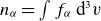 $n_\alpha =\int f_\alpha\, \text{d}^3v$
is the density, where
$n_\alpha =\int f_\alpha\, \text{d}^3v$
is the density, where $f_\alpha (\boldsymbol{x},\boldsymbol{v},t)$
is the particle distribution function, and the fluid flow velocity vector, pressure tensor and heat flux tensor components are defined by
$f_\alpha (\boldsymbol{x},\boldsymbol{v},t)$
is the particle distribution function, and the fluid flow velocity vector, pressure tensor and heat flux tensor components are defined by $u_{j,\alpha }=n_\alpha ^{-1} \int v_j f_\alpha\, \text{d}^3v$
,
$u_{j,\alpha }=n_\alpha ^{-1} \int v_j f_\alpha\, \text{d}^3v$
, $p_{jk,\alpha }=m_\alpha \int (v_j-u_j)(v_k-u_k) f_\alpha\,\text{d}^3v$
and
$p_{jk,\alpha }=m_\alpha \int (v_j-u_j)(v_k-u_k) f_\alpha\,\text{d}^3v$
and $q_{jkl,\alpha }=m_\alpha \int (v_j-u_j)(v_k-u_k)(v_l-u_l) f_\alpha\, \text{d}^3v$
, respectively. Furthermore,
$q_{jkl,\alpha }=m_\alpha \int (v_j-u_j)(v_k-u_k)(v_l-u_l) f_\alpha\, \text{d}^3v$
, respectively. Furthermore, $E_j$
and
$E_j$
and $B_j$
denote the electric and magnetic field components, which are evolved according to Maxwell’s equations,
$B_j$
denote the electric and magnetic field components, which are evolved according to Maxwell’s equations, $\partial _t \boldsymbol{B}=-\boldsymbol{\nabla }\times \boldsymbol{E}$
and
$\partial _t \boldsymbol{B}=-\boldsymbol{\nabla }\times \boldsymbol{E}$
and $\partial _t \boldsymbol{E}=c^2\boldsymbol{\nabla }\times \boldsymbol{B}-\epsilon _0^{-1}\sum _\alpha q_\alpha n_\alpha \boldsymbol{u}_\alpha$
. The solver uses a locally implicit scheme for the source terms, while solving the homogeneous portion of the equations by the wave propagation method (LeVeque Reference LeVeque1997). This approach allows certain unimportant scales to be under-resolved without leading to numerical difficulties. In particular, our simulations strongly under-resolve the Debye scale, which would not be possible in most particle-in-cell kinetic codes. This provides us greater flexibility in the plasma parameter regimes considered.
$\partial _t \boldsymbol{E}=c^2\boldsymbol{\nabla }\times \boldsymbol{B}-\epsilon _0^{-1}\sum _\alpha q_\alpha n_\alpha \boldsymbol{u}_\alpha$
. The solver uses a locally implicit scheme for the source terms, while solving the homogeneous portion of the equations by the wave propagation method (LeVeque Reference LeVeque1997). This approach allows certain unimportant scales to be under-resolved without leading to numerical difficulties. In particular, our simulations strongly under-resolve the Debye scale, which would not be possible in most particle-in-cell kinetic codes. This provides us greater flexibility in the plasma parameter regimes considered.
Importantly, the full pressure tensor is evolved for each species, which allows some pressure anisotropy driven instabilities (Gary Reference Gary1993) to be retained, such as the firehose instability (Walters et al. Reference Walters, Klein, Lichko, Juno and TenBarge2024) and, with particular relevance to the current work, the Weibel instability. Previous work by Kuldinow & Hara (Reference Kuldinow and Hara2025) employing the 10-moment system with a zero heat flux closure ( $q_{jkl}=0$
) demonstrated that the model can predict electron Weibel instability growth rates in the long wavelength and the strongly driven limits, and accurately reproduces the high wavenumber cutoff, as well as the nonlinear saturation level, of the instability.
$q_{jkl}=0$
) demonstrated that the model can predict electron Weibel instability growth rates in the long wavelength and the strongly driven limits, and accurately reproduces the high wavenumber cutoff, as well as the nonlinear saturation level, of the instability.
Here, we use a closure that drives the system towards an isotropic pressure (Wang et al. Reference Wang, Hakim, Bhattacharjee and Germaschewski2015)
 \begin{equation} \frac {\partial q_{jkl,\alpha }}{\partial x_l} = k_{0,\alpha } \frac {v_{\text{th},\alpha }}{\sqrt {2}} (p_{jk,\alpha } - p_\alpha \delta _{jk}), \end{equation}
where $p_\alpha =\delta _{lm}p_{lm,\alpha }/3$
is the scalar pressure and
$p_\alpha =\delta _{lm}p_{lm,\alpha }/3$
is the scalar pressure and $v_{\text{th},\alpha }=\sqrt {2 p_\alpha /(n_\alpha m_\alpha )}$
is the thermal speed. The parameters
$v_{\text{th},\alpha }=\sqrt {2 p_\alpha /(n_\alpha m_\alpha )}$
is the thermal speed. The parameters $k_{0,\alpha }$
adjust the strength of the isotropisation for each species. This isotropisation closure is not derived to capture a specific kinetic process (in contrast to, e.g. the Hammett–Perkins closure (Hammett & Perkins Reference Hammett and Perkins1990) for Landau damping) and the parameters
$k_{0,\alpha }$
adjust the strength of the isotropisation for each species. This isotropisation closure is not derived to capture a specific kinetic process (in contrast to, e.g. the Hammett–Perkins closure (Hammett & Perkins Reference Hammett and Perkins1990) for Landau damping) and the parameters $k_{0,\alpha }$
should therefore be regarded as free. However, by studying the parameters’ effect in a controlled manner, they can be used to approximate selected aspects of kinetic physics. In particular, as discussed in § 2.2, they regulate the damping of flows and magnetic fields in the unmagnetised limit, allowing one to emulate effective kinetic dissipation. In addition, as we show in Appendix A, the closure parameter can also be tuned to reproduce key characteristics of the electron Weibel instability. While other closures for the heat flux are available in Gkeyll, such as non-local (Ng et al. Reference Ng, Hakim, Bhattacharjee, Stanier and Daughton2017) or gradient-based (Ng et al. Reference Ng, Hakim, Wang and Bhattacharjee2020), we choose the local relaxation closure for its explicit connection to dissipation and our ability to determine effective Reynolds numbers from the choice of the closure parameter.
$k_{0,\alpha }$
should therefore be regarded as free. However, by studying the parameters’ effect in a controlled manner, they can be used to approximate selected aspects of kinetic physics. In particular, as discussed in § 2.2, they regulate the damping of flows and magnetic fields in the unmagnetised limit, allowing one to emulate effective kinetic dissipation. In addition, as we show in Appendix A, the closure parameter can also be tuned to reproduce key characteristics of the electron Weibel instability. While other closures for the heat flux are available in Gkeyll, such as non-local (Ng et al. Reference Ng, Hakim, Bhattacharjee, Stanier and Daughton2017) or gradient-based (Ng et al. Reference Ng, Hakim, Wang and Bhattacharjee2020), we choose the local relaxation closure for its explicit connection to dissipation and our ability to determine effective Reynolds numbers from the choice of the closure parameter.
2.2. Effect of closure parameters and effective Reynolds numbers
Unlike in resistive-MHD, where the concepts of dynamo theory have mostly been developed, in the 10-moment system, or a collisionless kinetic system for that matter, there is no explicit kinematic viscosity $\nu$
and magnetic diffusivity
$\nu$
and magnetic diffusivity $\eta$
. In addition, the corresponding damping rates of flow and magnetic perturbations can, in general, have different wavenumber (
$\eta$
. In addition, the corresponding damping rates of flow and magnetic perturbations can, in general, have different wavenumber ( $k$
) dependence to the
$k$
) dependence to the $\propto k^2$
diffusive behaviour. Thus, the usual definitions of the fluid and magnetic Reynolds numbers,
$\propto k^2$
diffusive behaviour. Thus, the usual definitions of the fluid and magnetic Reynolds numbers, $\textrm{Re}=u_0 L/\nu$
and
$\textrm{Re}=u_0 L/\nu$
and $\textrm{Rm}=u_0 L/\eta$
, respectively, are less trivial to evaluate,Footnote
4
and they have different implications concerning the scale separation between the outer scale and the fluctuation cutoff scales.
$\textrm{Rm}=u_0 L/\eta$
, respectively, are less trivial to evaluate,Footnote
4
and they have different implications concerning the scale separation between the outer scale and the fluctuation cutoff scales.
To put our results in context, it is nevertheless useful to quantify the magnetic and fluid damping in terms of analogous dimensionless quantities, comparing inverse time scales of processes creating and dissipating magnetic and fluid kinetic energy on the outer scale $L$
. The fluid Reynolds number compares inertial processes
$L$
. The fluid Reynolds number compares inertial processes ${\sim} u_0/L$
with (viscous) flow damping
${\sim} u_0/L$
with (viscous) flow damping ${\sim} \nu /L^2$
, while the magnetic Reynolds number compares field line stretching by the flow
${\sim} \nu /L^2$
, while the magnetic Reynolds number compares field line stretching by the flow ${\sim} u_0/L$
with resistive dissipation of magnetic fields
${\sim} u_0/L$
with resistive dissipation of magnetic fields ${\sim} \eta /L^2$
. Thus, a plausible generalisation of these quantities is
${\sim} \eta /L^2$
. Thus, a plausible generalisation of these quantities is
 \begin{equation} \textrm{Re} = \frac {u_0/L}{\left .\gamma _U^-\right |_{k_0}} \qquad \text{and} \qquad \textrm{Rm} = \frac {u_0/L}{\left .\gamma _B^-\right |_{k_0}}, \end{equation}
where $\left .\gamma _U^-\right |_{k_0}$
and
$\left .\gamma _U^-\right |_{k_0}$
and $\left .\gamma _B^-\right |_{k_0}$
are the damping rates of the mass flow and the magnetic field, respectively, taken at the wavenumber corresponding to the box scale
$\left .\gamma _B^-\right |_{k_0}$
are the damping rates of the mass flow and the magnetic field, respectively, taken at the wavenumber corresponding to the box scale $k=k_0\equiv 2\pi /L$
.
$k=k_0\equiv 2\pi /L$
.
In the following, we will show that in the 10-moment system employing the heat flux closure given in (2.4), the damping of the mass flow is governed by the ion closure parameter $k_{0,i}$
and the magnetic field damping by the electron closure parameter
$k_{0,i}$
and the magnetic field damping by the electron closure parameter $k_{0,e}$
. Specifically, the damping rate of the mass flow scales approximately as
$k_{0,e}$
. Specifically, the damping rate of the mass flow scales approximately as $\gamma _U^-\propto k^2/k_{0,i}$
, that is, with the same
$\gamma _U^-\propto k^2/k_{0,i}$
, that is, with the same $k$
-dependence as the diffusive flow damping in a viscous fluid. However, the damping rate of the magnetic field scales approximately as
$k$
-dependence as the diffusive flow damping in a viscous fluid. However, the damping rate of the magnetic field scales approximately as $\gamma _B^-\propto k^4/k_{0,e}$
, which is consistent with a hyperdiffusive damping. As we shall see, such separation of the electron and ion physics requires the mass ratio to be sufficiently large.
$\gamma _B^-\propto k^4/k_{0,e}$
, which is consistent with a hyperdiffusive damping. As we shall see, such separation of the electron and ion physics requires the mass ratio to be sufficiently large.
To establish how the damping of the mass flows and magnetic fields depend on the closure parameters, we have performed one-dimensional simulations initialised with sinusoidally varying, divergence-free perturbations of the respective quantities. The self-consistent exponential decay of these perturbations was used to fit flow and magnetic decay rates, $\gamma _U^-$
and
$\gamma _U^-$
and $\gamma _B^-$
. In particular, for the mass flow decay studies, the only non-vanishing component of the (equal) ion and electron flows are initially
$\gamma _B^-$
. In particular, for the mass flow decay studies, the only non-vanishing component of the (equal) ion and electron flows are initially $u_{\alpha z} = u_{\alpha z 0} \sin (k x)$
. For the magnetic decay studies, only the electrons have a non-zero initial velocity of the same form with a flow amplitude
$u_{\alpha z} = u_{\alpha z 0} \sin (k x)$
. For the magnetic decay studies, only the electrons have a non-zero initial velocity of the same form with a flow amplitude $u_{ez0}=B_{y0}k/(e\mu _0 n_e)$
, corresponding to a magnetic field perturbation
$u_{ez0}=B_{y0}k/(e\mu _0 n_e)$
, corresponding to a magnetic field perturbation $B_y = B_{y0} \cos (k x)$
. These simulations use the same linear box size as our dynamo simulations (namely,
$B_y = B_{y0} \cos (k x)$
. These simulations use the same linear box size as our dynamo simulations (namely, $L$
that defines
$L$
that defines $k_0=2\pi /L$
used for normalisation), while employing ten times higher resolution for improved accuracy.
$k_0=2\pi /L$
used for normalisation), while employing ten times higher resolution for improved accuracy.
Dependence of damping rates on closure parameters (circle markers, main figure) and wavenumber (diamond markers, inset figure). In both of these scans, star markers correspond to the baseline case. Dashed lines indicate fitted relevant power-law behaviour. (a) Mass flow damping rate as a function of $k_{0,i}/k_0$
and
$k_{0,i}/k_0$
and $k/k_0$
. (b) Magnetic field damping rate as a function of
$k/k_0$
. (b) Magnetic field damping rate as a function of $k_{0,e}/k_0$
and
$k_{0,e}/k_0$
and $k/k_0$
.
$k/k_0$
.

Figure 1 illustrates the numerically obtained dependencies of the damping rates in the vicinity of our baseline parameters (to be detailed in § 2.3). Over certain ranges, both $\gamma _U^-$
and
$\gamma _U^-$
and $\gamma _B^-$
are approximately inversely proportional to their respective closure parameter:
$\gamma _B^-$
are approximately inversely proportional to their respective closure parameter: $\gamma _U^-\propto k_{0,i}^{-1}$
and
$\gamma _U^-\propto k_{0,i}^{-1}$
and $\gamma _B^-\propto k_{0,e}^{-1}$
. For the flow damping, this dependence can be understood by a linearised analysis, with the assumptions that in the momentum equation, the
$\gamma _B^-\propto k_{0,e}^{-1}$
. For the flow damping, this dependence can be understood by a linearised analysis, with the assumptions that in the momentum equation, the $m_in_i\partial _t u_{iz}$
and
$m_in_i\partial _t u_{iz}$
and $\partial _x p_{ixz}$
terms nearly balance, while in the relevant
$\partial _x p_{ixz}$
terms nearly balance, while in the relevant $xz$
component of the pressure tensor equation, the generation of this off-diagonal pressure component by the term
$xz$
component of the pressure tensor equation, the generation of this off-diagonal pressure component by the term $p_{ixx}\partial _x u_{iz}$
is nearly compensated by its destruction by the isotropising closure term
$p_{ixx}\partial _x u_{iz}$
is nearly compensated by its destruction by the isotropising closure term $\propto v_{\textrm{th},i}k_{0,i}p_{ixz}$
. This behaviour yields a dependence of the damping rate
$\propto v_{\textrm{th},i}k_{0,i}p_{ixz}$
. This behaviour yields a dependence of the damping rate $\gamma _U^-\propto v_{\textrm {th},i} k^2/k_{0,i}$
, consistent with the scalings found in simulations around the baseline point. A somewhat more involved calculation of the magnetic damping rate, where Maxwell’s equations are also invoked in addition to the fluid ones, yields a similar regime
$\gamma _U^-\propto v_{\textrm {th},i} k^2/k_{0,i}$
, consistent with the scalings found in simulations around the baseline point. A somewhat more involved calculation of the magnetic damping rate, where Maxwell’s equations are also invoked in addition to the fluid ones, yields a similar regime $\gamma _B^-\propto v_{\textrm {th},e} k^4 \delta _e^2/k_{0,e}$
, where
$\gamma _B^-\propto v_{\textrm {th},e} k^4 \delta _e^2/k_{0,e}$
, where $\delta _\alpha =c/\omega _{p\alpha }$
denotes the inertial length and
$\delta _\alpha =c/\omega _{p\alpha }$
denotes the inertial length and $\omega _{p\alpha }=\sqrt {n_\alpha q_\alpha ^2/(\epsilon _0 m_\alpha )}$
the plasma frequency of species
$\omega _{p\alpha }=\sqrt {n_\alpha q_\alpha ^2/(\epsilon _0 m_\alpha )}$
the plasma frequency of species $\alpha$
. We note that this differs from the exact kinetic damping of magnetic fields (Mikhailovskii Reference Mikhailovskii1980; Pusztai et al. Reference Pusztai, Juno, Brandenburg, TenBarge, Hakim, Francisquez and Sundström2020), that is, of the form
$\alpha$
. We note that this differs from the exact kinetic damping of magnetic fields (Mikhailovskii Reference Mikhailovskii1980; Pusztai et al. Reference Pusztai, Juno, Brandenburg, TenBarge, Hakim, Francisquez and Sundström2020), that is, of the form $\gamma _B^-\propto v_{\textrm {th},e} k^3 \delta _e^2$
; thus, our closure introduces an extra
$\gamma _B^-\propto v_{\textrm {th},e} k^3 \delta _e^2$
; thus, our closure introduces an extra $k/k_{0,e}$
factor.
$k/k_{0,e}$
factor.
Clearly, the $1/k_{0,\alpha }$
scaling cannot hold for arbitrarily low values of the closure coefficients
$1/k_{0,\alpha }$
scaling cannot hold for arbitrarily low values of the closure coefficients $k_{0,\alpha }$
, because at low values, the damping rates saturate at a finite value. This behaviour can be seen for
$k_{0,\alpha }$
, because at low values, the damping rates saturate at a finite value. This behaviour can be seen for $\gamma _B^-$
in figure 1(b). In fact, box-scale magnetic perturbations at our baseline parameters are in the transition region to this saturation (while higher
$\gamma _B^-$
in figure 1(b). In fact, box-scale magnetic perturbations at our baseline parameters are in the transition region to this saturation (while higher $k$
values are typically in the
$k$
values are typically in the $\gamma _B^-\propto k_{0,e}^{-1}$
regime). However, increasing
$\gamma _B^-\propto k_{0,e}^{-1}$
regime). However, increasing $k_{0,e}$
brings our simulations away from this saturation, providing a reduced magnetic damping, which is essential for the interpretation of the dynamo results. Concerning flow damping, we observe the damping rate to level off also at high values of
$k_{0,e}$
brings our simulations away from this saturation, providing a reduced magnetic damping, which is essential for the interpretation of the dynamo results. Concerning flow damping, we observe the damping rate to level off also at high values of $k_{0,i}$
, and our baseline case is in this vicinity. It is of no concern though, as we do not perform scans in the ion closure parameter.
$k_{0,i}$
, and our baseline case is in this vicinity. It is of no concern though, as we do not perform scans in the ion closure parameter.
Mass-ratio dependence of the damping rate scaling exponents, defined through the power law relations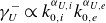 $\gamma _U^-\propto k_{0,i}^{\alpha _{U,i}}k_{0,e}^{\alpha _{U,e}}$
,
$\gamma _U^-\propto k_{0,i}^{\alpha _{U,i}}k_{0,e}^{\alpha _{U,e}}$
,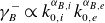 $\gamma _B^-\propto k_{0,i}^{\alpha _{B,i}}k_{0,e}^{\alpha _{B,e}}$
.
$\gamma _B^-\propto k_{0,i}^{\alpha _{B,i}}k_{0,e}^{\alpha _{B,e}}$
.

The effect of the mass ratio on the scaling of the damping rates is illustrated in figure 2 in terms of the exponents defined by
 \begin{equation} \gamma _U^-\propto k_{0,i}^{\alpha _{U,i}}k_{0,e}^{\alpha _{U,e}}k^{\alpha _{U,k}}, \qquad {} \gamma _B^-\propto k_{0,i}^{\alpha _{B,i}}k_{0,e}^{\alpha _{B,e}}k^{\alpha _{B,k}}. \end{equation}
We consider a starting point with parameters $k = k_0$
and
$k = k_0$
and $k_{0,i} = 13.6 k_0$
, as in our baseline case, and set
$k_{0,i} = 13.6 k_0$
, as in our baseline case, and set $k_{0,e} = 13.6 k_0$
to ensure consistency at unit mass ratio. The quantities
$k_{0,e} = 13.6 k_0$
to ensure consistency at unit mass ratio. The quantities $k_{0,i}$
,
$k_{0,i}$
, $k_{0,e}$
and
$k_{0,e}$
and $k$
are then perturbed about their baseline values in magnetic-field and mass-flow damping tests to determine the above-mentioned exponents. In all simulations, the electron mass is held fixed while the ion mass is varied.
$k$
are then perturbed about their baseline values in magnetic-field and mass-flow damping tests to determine the above-mentioned exponents. In all simulations, the electron mass is held fixed while the ion mass is varied.
The exponents characterising the $k$
dependence remain nearly constant over the entire mass-ratio scan, with
$k$
dependence remain nearly constant over the entire mass-ratio scan, with $\alpha _{U,k}\approx 2$
and
$\alpha _{U,k}\approx 2$
and $\alpha _{B,k}\approx 4$
, exhibiting maximum deviations of only
$\alpha _{B,k}\approx 4$
, exhibiting maximum deviations of only $1.2\,\,\%$
and
$1.2\,\,\%$
and $0.05\,\%$
, respectively. As these variations are negligible, the corresponding exponents are omitted from the figure. At unit mass ratio, the effects of ion (or, in this case, positron) and electron closures on the damping of a given quantity are identical, as expected. As the mass ratio increases,
$0.05\,\%$
, respectively. As these variations are negligible, the corresponding exponents are omitted from the figure. At unit mass ratio, the effects of ion (or, in this case, positron) and electron closures on the damping of a given quantity are identical, as expected. As the mass ratio increases, $\alpha _{U,i}$
and
$\alpha _{U,i}$
and $\alpha _{B,e}$
approach
$\alpha _{B,e}$
approach $-1$
, while
$-1$
, while $\alpha _{U,e}$
and
$\alpha _{U,e}$
and $\alpha _{B,i}$
approach
$\alpha _{B,i}$
approach $0$
. In other words, at sufficiently large mass ratio, magnetic-field damping depends solely on
$0$
. In other words, at sufficiently large mass ratio, magnetic-field damping depends solely on $k_{0,e}$
, whereas mass-flow damping depends solely on
$k_{0,e}$
, whereas mass-flow damping depends solely on $k_{0,i}$
, with cross-dependencies becoming negligible. This decoupling between electron and ion closures is already well converged at the mass ratio used in this study,
$k_{0,i}$
, with cross-dependencies becoming negligible. This decoupling between electron and ion closures is already well converged at the mass ratio used in this study, $m_i/m_e = 100$
. Finally, we note that over the mass-ratio range considered here, the sums
$m_i/m_e = 100$
. Finally, we note that over the mass-ratio range considered here, the sums $\alpha _{B,i} + \alpha _{U,i}$
and
$\alpha _{B,i} + \alpha _{U,i}$
and $\alpha _{B,e} + \alpha _{U,e}$
remain close to
$\alpha _{B,e} + \alpha _{U,e}$
remain close to $-1$
, with maximum deviations of
$-1$
, with maximum deviations of $1.9\,\%$
and
$1.9\,\%$
and $0.8\,\%$
, respectively.
$0.8\,\%$
, respectively.
Since the $k_{0,\alpha }\rightarrow 0$
limit of the 10-moment system is not singular, at sufficiently low values of the closure parameters
$k_{0,\alpha }\rightarrow 0$
limit of the 10-moment system is not singular, at sufficiently low values of the closure parameters $k_{0,\alpha }$
, these scalings must be broken and the damping rates saturate towards constant values. As seen in figure 1(b), we are in the vicinity of such a saturation concerning
$k_{0,\alpha }$
, these scalings must be broken and the damping rates saturate towards constant values. As seen in figure 1(b), we are in the vicinity of such a saturation concerning $\gamma _B^-(k_{0,e})$
at our baseline parameters; however, the scan in
$\gamma _B^-(k_{0,e})$
at our baseline parameters; however, the scan in $k_{0,e}$
we will perform moves deeper into the
$k_{0,e}$
we will perform moves deeper into the $\gamma _B^-\propto k_{0,e}^{-1}$
regime. Concerning the mass flows, we work in the
$\gamma _B^-\propto k_{0,e}^{-1}$
regime. Concerning the mass flows, we work in the $\gamma _U^-\propto k^2/k_{0,i}$
regime and we keep
$\gamma _U^-\propto k^2/k_{0,i}$
regime and we keep $k_{0,i}$
fixed.
$k_{0,i}$
fixed.
2.3. Simulation settings
To be relevant to the fast turbulent dynamo in collisionless astrophysical media, our simulations must have sustained three-dimensional flows. In reality, the flows are the result of gravitational collapse in the presence of dark matter, while our simulations include forced flows of non-gravitating baryonic matter in the plasma state. To produce a fast dynamo at a relatively low value of the critical magnetic Reynolds number, we drive our flows towards a simulation box-scale ( $L$
) Galloway–Proctor (GP) model flow (Galloway & Proctor Reference Galloway and Proctor1992). More specifically, both the electrons and ions are accelerated by the same spatio-temporally varying acceleration
$L$
) Galloway–Proctor (GP) model flow (Galloway & Proctor Reference Galloway and Proctor1992). More specifically, both the electrons and ions are accelerated by the same spatio-temporally varying acceleration $\boldsymbol{a}_\alpha (\boldsymbol{x},t)=C_f \boldsymbol{U}_{\textrm{GP}}(\boldsymbol{x},t)/t_{\text{str},i}$
, which is proportional to the GP flow,
$\boldsymbol{a}_\alpha (\boldsymbol{x},t)=C_f \boldsymbol{U}_{\textrm{GP}}(\boldsymbol{x},t)/t_{\text{str},i}$
, which is proportional to the GP flow,
 \begin{equation} \boldsymbol{U}_{\textrm {GP}}(\boldsymbol{x},t) = u_0 \left [ \begin{matrix} A \sin (k_0 z+\sin \omega t)+C \cos (k_0 y+\cos \omega t) \\[3pt] A \cos (k_0 z+\sin \omega t) \\[3pt] C \sin (k_0 y+\cos \omega t) \end{matrix} \right ], \end{equation}
where $t_{\text{str},i}=L/v_{\text{th},i}$
is the ion streaming time,
$t_{\text{str},i}=L/v_{\text{th},i}$
is the ion streaming time, $u_0$
is the nominal flow speed,
$u_0$
is the nominal flow speed, $k_0=2\pi /L$
is the lowest wavenumber fitting the simulation box, the constants
$k_0=2\pi /L$
is the lowest wavenumber fitting the simulation box, the constants $A$
and
$A$
and $C$
determining the stirring geometry are chosen to be unity here, while the constant
$C$
determining the stirring geometry are chosen to be unity here, while the constant $C_f$
sets the drive strength. In our baseline case, the representative flow speed is sub-sonic
$C_f$
sets the drive strength. In our baseline case, the representative flow speed is sub-sonic $u_0=0.35 c_s$
, with the sound speed
$u_0=0.35 c_s$
, with the sound speed $c_s=\sqrt {T_e/m_i}$
, which defines the outer turnover time
$c_s=\sqrt {T_e/m_i}$
, which defines the outer turnover time $t_{\text{turn}}=L/u_0$
. As this is expected to be the characteristic time scale of dynamo growth, we use
$t_{\text{turn}}=L/u_0$
. As this is expected to be the characteristic time scale of dynamo growth, we use $t_{\text{turn}}$
for time normalisation with the nominal flow speed
$t_{\text{turn}}$
for time normalisation with the nominal flow speed $u_0$
, while noting that the root mean square flow speed varies over time and is in general different from
$u_0$
, while noting that the root mean square flow speed varies over time and is in general different from $u_0$
. We also set the stirring frequency of the flow to
$u_0$
. We also set the stirring frequency of the flow to $\omega =2\pi /t_{\text{turn}}$
.
$\omega =2\pi /t_{\text{turn}}$
.
The simulations use a mass ratio of $m_i/m_e=100$
, and our baseline driving strength of
$m_i/m_e=100$
, and our baseline driving strength of $C_f=2$
and
$C_f=2$
and $k_{0,i}=13.6 k_0$
are chosen such that the flows remain subsonic throughout the simulation. As a reference, this value of
$k_{0,i}=13.6 k_0$
are chosen such that the flows remain subsonic throughout the simulation. As a reference, this value of $k_{0,i}$
corresponds to
$k_{0,i}$
corresponds to $\textrm{Re}= 0.535$
, while
$\textrm{Re}= 0.535$
, while $k_{0,e}=1 k_0$
corresponds to
$k_{0,e}=1 k_0$
corresponds to $\textrm{Rm}= 307$
, according to numerical damping rate tests like those presented in § 2.2, yielding a large magnetic Prandtl number
$\textrm{Rm}= 307$
, according to numerical damping rate tests like those presented in § 2.2, yielding a large magnetic Prandtl number $\textrm{Pm}= \textrm{Rm}/\textrm{Re}=574$
, which is relevant for the ICM. Due to numerical limitations on achievable scale separations, our approach to the
$\textrm{Pm}= \textrm{Rm}/\textrm{Re}=574$
, which is relevant for the ICM. Due to numerical limitations on achievable scale separations, our approach to the $\textrm{Pm}\gg 1$
limit sacrifices the fluid cascade and modelling the system at the viscous cutoff scale. This limitation results in smooth, large-scale flows with a rapidly decaying velocity spectrum, i.e. a form of turbulence that lacks an extended inertial range due to strong damping at small scales. Despite the absence of an extended inertial range, such flows can still sustain dynamo amplification through coherent stretching (Schekochihin et al. Reference Schekochihin, Cowley, Taylor, Maron and McWilliams2004). Moreover, it is worth emphasising that the dissipation in a collisionless system is not expected to be fixed: it evolves as the plasma becomes increasingly magnetised and is further modified by kinetic instabilities.
$\textrm{Pm}\gg 1$
limit sacrifices the fluid cascade and modelling the system at the viscous cutoff scale. This limitation results in smooth, large-scale flows with a rapidly decaying velocity spectrum, i.e. a form of turbulence that lacks an extended inertial range due to strong damping at small scales. Despite the absence of an extended inertial range, such flows can still sustain dynamo amplification through coherent stretching (Schekochihin et al. Reference Schekochihin, Cowley, Taylor, Maron and McWilliams2004). Moreover, it is worth emphasising that the dissipation in a collisionless system is not expected to be fixed: it evolves as the plasma becomes increasingly magnetised and is further modified by kinetic instabilities.
Unlike particle-in-cell simulations, the continuum solvers of Gkeyll are essentially noise-free, thus we need to prescribe magnetic perturbations from which the Weibel instability can grow. Note that due to the rapid growth of this instability, the fact that we need such a seed magnetic field is not an issue, as in astrophysical settings, the instability would produce macroscopic field strengths from arbitrarily small fluctuations on time scales shorter than those of the dynamo growth. Thus, as an initial condition, we prescribe a magnetic field of the form
 \begin{equation} B_{i}(t=0)=B_0 \sum _{j\ne i,n} b_{ij,n}\cos [n k_0 (x_j+L\phi _{ij,n})], \end{equation}
with random relative amplitudes $b_{ij,n}$
and phases
$b_{ij,n}$
and phases $\phi _{ij,n}$
, both uniform on the unit interval, and a characteristic magnetic field strength
$\phi _{ij,n}$
, both uniform on the unit interval, and a characteristic magnetic field strength $B_0$
. Here, we only seed the four lowest mode numbers
$B_0$
. Here, we only seed the four lowest mode numbers $n$
. For our initial nominal field
$n$
. For our initial nominal field $B=B_0$
, the thermal electron Larmor radius
$B=B_0$
, the thermal electron Larmor radius $\rho _e=v_{\text{th},e} m_e/(e B)$
is
$\rho _e=v_{\text{th},e} m_e/(e B)$
is $\rho _e=4.4 L$
, thus the system is non-magnetised. The system is non-relativistic, since
$\rho _e=4.4 L$
, thus the system is non-magnetised. The system is non-relativistic, since $v_{\text{th},e}/c=0.0625$
.
$v_{\text{th},e}/c=0.0625$
.
A current consistent with this field, $\boldsymbol{j}=\mu _0^{-1}\boldsymbol{\nabla }\times \boldsymbol{B}$
, fully carried by the electrons, is also prescribed. In addition, there is an initial flow velocity, equal for the electrons and the ions, given by (2.7) for
$\boldsymbol{j}=\mu _0^{-1}\boldsymbol{\nabla }\times \boldsymbol{B}$
, fully carried by the electrons, is also prescribed. In addition, there is an initial flow velocity, equal for the electrons and the ions, given by (2.7) for $t=0$
. The initial ratio of the box-integrated magnetic energy and kinetic energy in the flows is
$t=0$
. The initial ratio of the box-integrated magnetic energy and kinetic energy in the flows is $3.7\times 10^{-6}$
. Our baseline box size is
$3.7\times 10^{-6}$
. Our baseline box size is $L=70 \delta _i$
in each direction. With a spatial resolution of
$L=70 \delta _i$
in each direction. With a spatial resolution of $N=140$
in each direction, such that the linear size of the finite volume is
$N=140$
in each direction, such that the linear size of the finite volume is $\varDelta x=L/140$
, the ion inertial length is barely resolved
$\varDelta x=L/140$
, the ion inertial length is barely resolved $\delta _i=2\varDelta x$
, while the electron inertial length is under-resolved
$\delta _i=2\varDelta x$
, while the electron inertial length is under-resolved $\delta _e=0.2\varDelta x$
, along with the Debye length
$\delta _e=0.2\varDelta x$
, along with the Debye length $\lambda _D\equiv \sqrt {\epsilon _0 T_e/(n_e e^2)}\approx 0.009\varDelta x$
. These scales are not a concern since the Debye scale is not playing an important role in the physics of the system, and the characteristic scales of the electron Weibel instability are significantly larger than
$\lambda _D\equiv \sqrt {\epsilon _0 T_e/(n_e e^2)}\approx 0.009\varDelta x$
. These scales are not a concern since the Debye scale is not playing an important role in the physics of the system, and the characteristic scales of the electron Weibel instability are significantly larger than $\delta _e$
due to the weak pressure anisotropy that develops in the system.
$\delta _e$
due to the weak pressure anisotropy that develops in the system.
We finally note that our simulations are performed in SI units with physical parameters comparable to those of Pusztai et al. (Reference Pusztai, Juno, Brandenburg, TenBarge, Hakim, Francisquez and Sundström2020). Namely, all physical constants have their actual value, except the ion mass that is $m_i=100 m_e$
; both species have initially the same scalar temperature
$m_i=100 m_e$
; both species have initially the same scalar temperature $T_e=T_i=1\,\textrm {keV}$
, the electron density is
$T_e=T_i=1\,\textrm {keV}$
, the electron density is $n_e=2.3 \times 10^{28} \,\textrm {m}^{-3}$
, along with
$n_e=2.3 \times 10^{28} \,\textrm {m}^{-3}$
, along with $k_0=2.58 \times 10^5\,\textrm {m}^{-1}$
. Furthermore,
$k_0=2.58 \times 10^5\,\textrm {m}^{-1}$
. Furthermore, $B_0=1\,\textrm {T}$
. As the system has the scale invariance of a collisionless kinetic system, the fact that the plasma parameters (particularly the density) are not representative of the ICM is of no concern; we will present our results with practical normalisations.
$B_0=1\,\textrm {T}$
. As the system has the scale invariance of a collisionless kinetic system, the fact that the plasma parameters (particularly the density) are not representative of the ICM is of no concern; we will present our results with practical normalisations.
2.4. Electron Weibel instability in non-magnetised collisionless plasma turbulence
The Weibel instability is a non-magnetised kinetic plasma instability that arises in the presence of an anisotropic velocity distribution. Transverse perturbations in the magnetic field deflect particles in a way that produces currents reinforcing the perturbation. As a result, it tends to generate filamentary current and magnetic field structures, and acts to restore pressure isotropy. It plays important roles in astrophysical and laboratory plasmas (e.g. collisionless shocks, gamma-ray bursts, laser-plasma experiments) by generating sizable magnetic fields in initially non-magnetised or weakly magnetised environments, thereby qualitatively affecting particle dynamics. The instability has both electron and ion variants, and additionally arises in pair-plasmas.
A large body of the Weibel literature is concerned with interpenetrating (often supersonic and relativistic) flow scenarios, due to its relevance for collisionless astrophysical shocks (Medvedev & Loeb Reference Medvedev and Loeb1999; Medvedev, Silva & Kamionkowski Reference Medvedev, Silva and Kamionkowski2006; Spitkovsky Reference Spitkovsky2007; Kato & Takabe Reference Kato and Takabe2008), such as supernova remnants, and laser-plasma experiments (Schoeffler et al. Reference Schoeffler, Loureiro, Fonseca and Silva2014; Huntington et al. Reference Huntington2015). Pressure anisotropies appearing in such scenarios are typically substantial. However, as demonstrated by Zhou et al. (Reference Zhou, Zhdankin, Kunz, Loureiro and Uzdensky2022), the Weibel instability also naturally occurs in non-magnetised collisionless plasma turbulence, since phase mixing in sheared flows creates pressure anisotropy $\varDelta _\alpha$
. For subsonic turbulence, as relevant for our topic, this anisotropy is small (see Appendix B for representative values from our simulations).
$\varDelta _\alpha$
. For subsonic turbulence, as relevant for our topic, this anisotropy is small (see Appendix B for representative values from our simulations).
The intuitive and conventional definition $\varDelta _\alpha =p_{\|\alpha }/p_{\perp \alpha }-1$
implicitly assumes a pressure tensor with diagonal components
$\varDelta _\alpha =p_{\|\alpha }/p_{\perp \alpha }-1$
implicitly assumes a pressure tensor with diagonal components $\{p_{\|\alpha }, p_{\perp \alpha },p_{\perp \alpha }\}$
; this definition will need to be revised, since the pressure tensor in a non-magnetised system is non-gyrotropic and has, in general, three distinct eigenvalues. Thus, following Zhou et al. (Reference Zhou, Zhdankin, Kunz, Loureiro and Uzdensky2022), we use the definition
$\{p_{\|\alpha }, p_{\perp \alpha },p_{\perp \alpha }\}$
; this definition will need to be revised, since the pressure tensor in a non-magnetised system is non-gyrotropic and has, in general, three distinct eigenvalues. Thus, following Zhou et al. (Reference Zhou, Zhdankin, Kunz, Loureiro and Uzdensky2022), we use the definition $\varDelta _\alpha =\sqrt {\langle (p_{\textrm{max},\alpha }/p_{\textrm {min}, \alpha} )^2\rangle }-1$
, where
$\varDelta _\alpha =\sqrt {\langle (p_{\textrm{max},\alpha }/p_{\textrm {min}, \alpha} )^2\rangle }-1$
, where $p_{\textrm {max},\alpha}$
is the highest eigenvalue of the pressure tensor,
$p_{\textrm {max},\alpha}$
is the highest eigenvalue of the pressure tensor, $p_{\textrm {min},\alpha}$
is the average of the two lower eigenvalues and the angle bracket denotes the spatial (box) average.
$p_{\textrm {min},\alpha}$
is the average of the two lower eigenvalues and the angle bracket denotes the spatial (box) average.
Since the pressure anisotropies of ions and electrons that develop in the sheared flow tend to be comparable, the electron Weibel instability will dominate the magnetic field growth as it has higher growth rates than the ion mode. Specifically, in terms of the above-mentioned anisotropy measure that is positive by construction, the fastest growing electron Weibel mode has a characteristic wavenumber $k\sim \varDelta _e^{1/2}/\delta _e$
and a growth rate of
$k\sim \varDelta _e^{1/2}/\delta _e$
and a growth rate of $\gamma _B \sim \varDelta _e^{3/2}\omega _{pe}v_{\text{th},e}/c$
. For
$\gamma _B \sim \varDelta _e^{3/2}\omega _{pe}v_{\text{th},e}/c$
. For $\varDelta _e \ll 1$
, the characteristic wavenumber is shifted to scales larger than the electron inertial length.
$\varDelta _e \ll 1$
, the characteristic wavenumber is shifted to scales larger than the electron inertial length.
3. Results
3.1. Baseline case
First, we consider results for our baseline case with parameters given in § 2.3, to establish the qualitative features of a representative simulation, before we consider the effect of the electron closure parameter and the box size in the following subsections.
The total magnetic field energy evolution is clearly separated into three phases, as shown in figure 3(a) (solid black line, $E_B$
). The first, very short phase,
$E_B$
). The first, very short phase, $t/t_{\text{turn}} \lt 0.1$
, characterised by a very rapid magnetic field growth, is dominated by the electron Weibel instability. This phase is followed by a nearly exponential growth with a growth rate comparable to the outer turnover time, approximately
$t/t_{\text{turn}} \lt 0.1$
, characterised by a very rapid magnetic field growth, is dominated by the electron Weibel instability. This phase is followed by a nearly exponential growth with a growth rate comparable to the outer turnover time, approximately $\gamma _B t_{\text{turn}} = 0.76$
, as indicated by the dotted line, which abruptly saturates around
$\gamma _B t_{\text{turn}} = 0.76$
, as indicated by the dotted line, which abruptly saturates around $t/t_{\text{turn}} = 3.4$
. As the magnetic energy approaches the kinetic energy in the flow
$t/t_{\text{turn}} = 3.4$
. As the magnetic energy approaches the kinetic energy in the flow $E_U$
(dashed black line), the magnetic field brakes the flow and the flow energy drops, until eventually, the two forms of energy establish near equipartition. It is noteworthy that the dynamo growth rate appears to increase towards the end of the growth phase even though the flow energy slowly decreases in time. This behaviour could be caused by the increasing magnetisation of the plasma leading to a reduced kinetic magnetic field damping.
$E_U$
(dashed black line), the magnetic field brakes the flow and the flow energy drops, until eventually, the two forms of energy establish near equipartition. It is noteworthy that the dynamo growth rate appears to increase towards the end of the growth phase even though the flow energy slowly decreases in time. This behaviour could be caused by the increasing magnetisation of the plasma leading to a reduced kinetic magnetic field damping.
The qualitative behaviour is quite similar to that observed in kinetic simulations of pair-plasma dynamos by Zhou et al. (Reference Zhou, Zhdankin, Kunz, Loureiro and Uzdensky2023), such as the case shown in their figure 1(a). In addition to observing the same main phases of the magnetic field evolution, we also find that, in spite of the steady forcing of the flow, the flow energy decreases after a time comparable with $t_{\text{turn}}$
, before it finds its long time quasi-equilibrium value. However, in the results here, as a consequence of driving a flow towards the GP model flow instead of a random flow drive, the contribution of the
$t_{\text{turn}}$
, before it finds its long time quasi-equilibrium value. However, in the results here, as a consequence of driving a flow towards the GP model flow instead of a random flow drive, the contribution of the $x$
-component of the flow to the kinetic energy is larger than that of the other directions, as seen by comparing the red dashed curve (
$x$
-component of the flow to the kinetic energy is larger than that of the other directions, as seen by comparing the red dashed curve ( $x$
-component) to the blue and green curves (
$x$
-component) to the blue and green curves ( $y$
- and
$y$
- and $z$
-components).
$z$
-components).
The time evolution of the magnetic energy wavenumber spectra is shown in figure 3(b). After $t=0$
, where the magnetic field is seeded only up to
$t=0$
, where the magnetic field is seeded only up to $k/k_0=4$
, the first time point shown is already after the Weibel phase and its high-
$k/k_0=4$
, the first time point shown is already after the Weibel phase and its high- $k$
range is dominated by a peak corresponding to magnetic energy created by the Weibel instability. The spectral peak then moves towards lower
$k$
range is dominated by a peak corresponding to magnetic energy created by the Weibel instability. The spectral peak then moves towards lower $k$
, until the magnetic energy at the lowest wave number (
$k$
, until the magnetic energy at the lowest wave number ( $k=k_0$
) takes over. Eventually, most of the spectrum becomes power-law-like, comparable to
$k=k_0$
) takes over. Eventually, most of the spectrum becomes power-law-like, comparable to $k^{-5.5}$
(as indicated by the dotted line), while the lowermost
$k^{-5.5}$
(as indicated by the dotted line), while the lowermost $k$
range, up to around
$k$
range, up to around $4k_0$
, exhibits a less steep spectrum, approximately
$4k_0$
, exhibits a less steep spectrum, approximately $k^{-1.6}$
.
$k^{-1.6}$
.
Magnetic field generation in the simulation with the baseline parameters. (a) Time evolution of the box-integrated magnetic energy $E_B$
(solid black curve) and kinetic energy in the flows
$E_B$
(solid black curve) and kinetic energy in the flows $E_U$
(dashed black), normalised to the initial value of
$E_U$
(dashed black), normalised to the initial value of $E_U$
. With similar line styles, contributions from the
$E_U$
. With similar line styles, contributions from the $\{x, y, z\}$
components of
$\{x, y, z\}$
components of $\boldsymbol{U}$
and
$\boldsymbol{U}$
and $\boldsymbol{B}$
are shown in red, blue and green, respectively. The dotted line corresponds to an exponential growth of the magnetic field with a growth rate of
$\boldsymbol{B}$
are shown in red, blue and green, respectively. The dotted line corresponds to an exponential growth of the magnetic field with a growth rate of $\gamma _B t_{\text{turn}} = 0.76$
. (b) Wavenumber spectra of the magnetic field energy. The wavenumber
$\gamma _B t_{\text{turn}} = 0.76$
. (b) Wavenumber spectra of the magnetic field energy. The wavenumber $k$
is normalised to
$k$
is normalised to $k_0$
and the spectrum is normalised to its value at
$k_0$
and the spectrum is normalised to its value at $k=k_0$
for
$k=k_0$
for $t=0$
. For reference, the dotted line indicates a power law
$t=0$
. For reference, the dotted line indicates a power law $k^{-5.5}$
.
$k^{-5.5}$
.

Time evolution during the Weibel instability phase. (a) Dimensionless quantities: pressure anisotropy of electrons (blue, $\varDelta _e$
) and ions (red,
$\varDelta _e$
) and ions (red, $\varDelta _i$
), normalised magnetic field energy (green,
$\varDelta _i$
), normalised magnetic field energy (green, $\beta _e^{-1}$
), and instantaneous magnetic field growth rate (purple,
$\beta _e^{-1}$
), and instantaneous magnetic field growth rate (purple, $\gamma _B/\omega _{pe}$
). (b) Instantaneous magnetic growth rate spectra (
$\gamma _B/\omega _{pe}$
). (b) Instantaneous magnetic growth rate spectra ( $\gamma _Bt_{\text{turn}}$
) for several time instances (colour coded from blue to yellow for increasing time) across the time period of the fastest field growth, bound by the dotted vertical lines of panel (a). The black curve corresponds to the time of fastest global magnetic field growth, indicated by the solid vertical line in panel (a). The dotted horizontal and the dashed vertical line correspond to
$\gamma _Bt_{\text{turn}}$
) for several time instances (colour coded from blue to yellow for increasing time) across the time period of the fastest field growth, bound by the dotted vertical lines of panel (a). The black curve corresponds to the time of fastest global magnetic field growth, indicated by the solid vertical line in panel (a). The dotted horizontal and the dashed vertical line correspond to $\gamma _B=\varDelta _e^{3/2}\omega _{pe}v_{\text{th},e}/c$
and
$\gamma _B=\varDelta _e^{3/2}\omega _{pe}v_{\text{th},e}/c$
and $k=\varDelta _e^{1/2}/\delta _e$
, respectively.
$k=\varDelta _e^{1/2}/\delta _e$
, respectively.

The dynamics of the system during the short Weibel period is illustrated in figure 4(a), which contains similar information to figure 2 of Zhou et al. (Reference Zhou, Zhdankin, Kunz, Loureiro and Uzdensky2022). The magnetic energy, now quantified via $\beta _e^{-1}$
(green curve) undergoes a very rapid growth phase approximately bounded by the dotted vertical lines, with the instantaneous growth rate of the magnetic field (
$\beta _e^{-1}$
(green curve) undergoes a very rapid growth phase approximately bounded by the dotted vertical lines, with the instantaneous growth rate of the magnetic field ( $\gamma _B$
, purple) peaking just before
$\gamma _B$
, purple) peaking just before $t/t_{\text{turn}}=0.04$
, marked by the solid line. Initially, the pressure anisotropies of both species are growing in accordance with the sheared flow that is present in the system already from
$t/t_{\text{turn}}=0.04$
, marked by the solid line. Initially, the pressure anisotropies of both species are growing in accordance with the sheared flow that is present in the system already from $t=0$
. When the growth rate peaks, the instability becomes strong enough that it starts to back-react on its drive, the electron pressure anisotropy (
$t=0$
. When the growth rate peaks, the instability becomes strong enough that it starts to back-react on its drive, the electron pressure anisotropy ( $\varDelta _e$
, blue). Here,
$\varDelta _e$
, blue). Here, $\varDelta _e$
declines somewhat to eventually stabilise at a lower level. Meanwhile, the steady growth of the ion pressure anisotropy (
$\varDelta _e$
declines somewhat to eventually stabilise at a lower level. Meanwhile, the steady growth of the ion pressure anisotropy ( $\varDelta _i$
, red) remains unaffected by the instability, providing one piece of evidence that the instability is indeed driven by
$\varDelta _i$
, red) remains unaffected by the instability, providing one piece of evidence that the instability is indeed driven by $\varDelta _e$
. More details on the long-time evolution of the system in terms of electron pressure anisotropy and normalised pressure are provided in Appendix B.
$\varDelta _e$
. More details on the long-time evolution of the system in terms of electron pressure anisotropy and normalised pressure are provided in Appendix B.
The wavenumber-resolved instantaneous growth rates of the magnetic field are shown for a range of time points in figure 4(b). At the approximate time of fastest global magnetic energy growth, corresponding to the thick black line, the peak of the growth rate spectrum is located in the vicinity of $k=\varDelta _e^{1/2}/\delta _e$
and takes a value comparable to
$k=\varDelta _e^{1/2}/\delta _e$
and takes a value comparable to $\gamma _B=\varDelta _e^{3/2}\omega _{pe}v_{\text{th},e}/c$
, indicated by the dashed vertical and the dotted horizontal lines, respectively. These are the theoretical scalings from Zhou et al. (Reference Zhou, Zhdankin, Kunz, Loureiro and Uzdensky2023), without their specific order unity prefactors. The purpose of these is just to illustrate that the magnetic field growth is consistent with being produced by the electron Weibel instability. An accurate numerical comparison would require theory for a system similar to our simulated scenario, but even then, differences due to our simulation being fluid are expected.
$\gamma _B=\varDelta _e^{3/2}\omega _{pe}v_{\text{th},e}/c$
, indicated by the dashed vertical and the dotted horizontal lines, respectively. These are the theoretical scalings from Zhou et al. (Reference Zhou, Zhdankin, Kunz, Loureiro and Uzdensky2023), without their specific order unity prefactors. The purpose of these is just to illustrate that the magnetic field growth is consistent with being produced by the electron Weibel instability. An accurate numerical comparison would require theory for a system similar to our simulated scenario, but even then, differences due to our simulation being fluid are expected.
Magnitude of the magnetic field in 2-D cuts of the simulation domain, taken (a) and (d) at the time of the fastest magnetic growth during the Weibel phase, $t/t_{\text{turn}}=0.038$
, (b) and (e) in the middle of the dynamo growth phase,
$t/t_{\text{turn}}=0.038$
, (b) and (e) in the middle of the dynamo growth phase, $t/t_{\text{turn}}=2.0$
, and (c) and (f) in the saturated phase,
$t/t_{\text{turn}}=2.0$
, and (c) and (f) in the saturated phase, $t/t_{\text{turn}}=10.0$
. Panels (a–c) are cuts at
$t/t_{\text{turn}}=10.0$
. Panels (a–c) are cuts at $x=L/2$
, while panels (d–f) are cuts at
$x=L/2$
, while panels (d–f) are cuts at $y=L/2$
(the latter are morphologically similar to constant
$y=L/2$
(the latter are morphologically similar to constant $z$
cuts, not shown). The normalising ‘equipartition’ magnetic field
$z$
cuts, not shown). The normalising ‘equipartition’ magnetic field $B_{\textrm {eq}}$
is defined such that
$B_{\textrm {eq}}$
is defined such that $B_{\textrm {eq}}^2/(2\mu _0)$
equals the box-averaged kinetic energy density in the bulk flows at
$B_{\textrm {eq}}^2/(2\mu _0)$
equals the box-averaged kinetic energy density in the bulk flows at $t=0$
.
$t=0$
.

The morphology of the magnetic field strength is shown in figure 5 for the three phases of the magnetic field evolution. The left panels, taken at the time of fastest magnetic growth in the Weibel phase, show characteristic Weibel filamentation coincident with the regions of strongest shear in the GP flow structure (stream plotted with white arrows). Recall from (2.7) that the flow is independent of $x$
, and it forms two circulations in the
$x$
, and it forms two circulations in the $y$
–
$y$
– $z$
plane around the elliptic fixed points located at
$z$
plane around the elliptic fixed points located at $\{z,y\}\approx \{0.25,0.84\}$
and
$\{z,y\}\approx \{0.25,0.84\}$
and $\{z,y\}\approx \{0.75,0.34\}$
. In these nearly circular regions, the magnetic field remains relatively low, with some structure around the boundary of the circulations, as shown in figure 5(a). The strongest magnetic energy growth is instead observed in the vicinity of the hyperbolic fixed points located around
$\{z,y\}\approx \{0.75,0.34\}$
. In these nearly circular regions, the magnetic field remains relatively low, with some structure around the boundary of the circulations, as shown in figure 5(a). The strongest magnetic energy growth is instead observed in the vicinity of the hyperbolic fixed points located around $\{z,y\}\approx \{0.25,0.34\}$
and
$\{z,y\}\approx \{0.25,0.34\}$
and $\{z,y\}\approx \{0.75,0.84\}$
. It is in fact in these regions where the shear strain of the flow is strongest.Footnote
5
In this
$\{z,y\}\approx \{0.75,0.84\}$
. It is in fact in these regions where the shear strain of the flow is strongest.Footnote
5
In this $z$
–
$z$
– $y$
plane, the magnetic filaments are aligned parallel to the unstable separatrix. In the
$y$
plane, the magnetic filaments are aligned parallel to the unstable separatrix. In the $z$
-
$z$
- $x$
plane, figure 5(d), the same filaments, which form planar structures in three dimensions, are elongated along the
$x$
plane, figure 5(d), the same filaments, which form planar structures in three dimensions, are elongated along the $x$
direction, best seen around
$x$
direction, best seen around $z=0.25$
, which is close to one of the highly strained regions. In the rest of the plane, the striations are elongated mostly in the
$z=0.25$
, which is close to one of the highly strained regions. In the rest of the plane, the striations are elongated mostly in the $z$
direction; they have longer wavelengths and are caused by the sheared flows in the
$z$
direction; they have longer wavelengths and are caused by the sheared flows in the $x$
-direction.
$x$
-direction.
In the dynamo growth phase, shown in figure 5(b) and 5(e), the localised fine scale striations corresponding to the electron Weibel instability disappear and no clear directionality is left in the $z$
–
$z$
– $y$
plane. The characteristic scale of the fluctuations is clearly larger than that of the Weibel striations. Due to the special form of the flow forcing, the fluctuations are not completely isotropic even in the
$y$
plane. The characteristic scale of the fluctuations is clearly larger than that of the Weibel striations. Due to the special form of the flow forcing, the fluctuations are not completely isotropic even in the $z$
–
$z$
– $y$
plane, rather some structure appears to be aligned with the coordinate axes. This preferential alignment in the
$y$
plane, rather some structure appears to be aligned with the coordinate axes. This preferential alignment in the $z$
–
$z$
– $y$
plane is not apparent in the saturated state, shown in figures 5(c) and 5(f). However, there is an alignment with the special direction
$y$
plane is not apparent in the saturated state, shown in figures 5(c) and 5(f). However, there is an alignment with the special direction $x$
, which, being a symmetry direction of the forcing, consistently supports the strongest flows (as also seen by comparing the corresponding flow energies: the red dashed curve to the blue and green ones in figure 3
a).
$x$
, which, being a symmetry direction of the forcing, consistently supports the strongest flows (as also seen by comparing the corresponding flow energies: the red dashed curve to the blue and green ones in figure 3
a).
3.2. Increased electron pressure isotropisation
We will now consider the effect of increasing electron pressure isotropisation from its baseline value $k_{0,e}/k_0=1$
. Information similar to that in figure 3, but for
$k_{0,e}/k_0=1$
. Information similar to that in figure 3, but for $k_{0,e}/k_0=\{2,\,4,\,8,\,32\}$
, is shown in figure 6. As the strength of the isotropisation is increased, and thus the drive of the Weibel instability is reduced, we observe a diminishing Weibel growth phase. Up to the
$k_{0,e}/k_0=\{2,\,4,\,8,\,32\}$
, is shown in figure 6. As the strength of the isotropisation is increased, and thus the drive of the Weibel instability is reduced, we observe a diminishing Weibel growth phase. Up to the $k_{0,e}/k_0=4$
case, we still observe a magnetic growth rate that increases in time during the otherwise nearly exponential dynamo growth phase, but it is not present in the higher
$k_{0,e}/k_0=4$
case, we still observe a magnetic growth rate that increases in time during the otherwise nearly exponential dynamo growth phase, but it is not present in the higher $k_{0,e}$
cases. Perhaps more importantly, the representative growth rate increases with increasing
$k_{0,e}$
cases. Perhaps more importantly, the representative growth rate increases with increasing $k_{0,e}$
, as indicated by the dotted lines and
$k_{0,e}$
, as indicated by the dotted lines and $\gamma _Bt_{\text{turn}}$
values in the figure. This behaviour is consistent with the magnetic damping decreasing as
$\gamma _Bt_{\text{turn}}$
values in the figure. This behaviour is consistent with the magnetic damping decreasing as $1/k_{0,e}$
. To draw an analogy with the dynamo in resistive magnetohydrodynamics, we may think of the reduced magnetic damping as an increased magnetic Reynolds number. A fast dynamo produces an increasing and eventually saturated growth rate with increasing magnetic Reynolds number, which is qualitatively consistent with the increasing
$1/k_{0,e}$
. To draw an analogy with the dynamo in resistive magnetohydrodynamics, we may think of the reduced magnetic damping as an increased magnetic Reynolds number. A fast dynamo produces an increasing and eventually saturated growth rate with increasing magnetic Reynolds number, which is qualitatively consistent with the increasing $\gamma _B$
we observe for increasing
$\gamma _B$
we observe for increasing $k_{0,e}$
.
$k_{0,e}$
.
Magnetic field generation in simulations using $k_{0,e}/k_0=\{2,\,4,\,8,\,32\}$
, shown in different rows. Left column: time evolution of the box-integrated magnetic energy
$k_{0,e}/k_0=\{2,\,4,\,8,\,32\}$
, shown in different rows. Left column: time evolution of the box-integrated magnetic energy $E_B$
(solid black curve) and kinetic energy in the flows
$E_B$
(solid black curve) and kinetic energy in the flows $E_U$
(dashed black), normalised to the initial value of
$E_U$
(dashed black), normalised to the initial value of $E_U$
. With similar line styles, contributions from the
$E_U$
. With similar line styles, contributions from the $\{x, y, z\}$
components of
$\{x, y, z\}$
components of $\boldsymbol{U}$
and
$\boldsymbol{U}$
and $\boldsymbol{B}$
are shown in red, blue and green, respectively. Exponential magnetic growth is indicated by dotted lines with growth rates provided in the figure. Right column: wave number spectra of the magnetic field energy. The wave number
$\boldsymbol{B}$
are shown in red, blue and green, respectively. Exponential magnetic growth is indicated by dotted lines with growth rates provided in the figure. Right column: wave number spectra of the magnetic field energy. The wave number $k$
is normalised to
$k$
is normalised to $k_0$
and the spectra are normalised to its value at
$k_0$
and the spectra are normalised to its value at $k=k_0$
for
$k=k_0$
for $t=0$
. Dotted lines indicate power laws for reference.
$t=0$
. Dotted lines indicate power laws for reference.

Similar to the $k_{0,e}/k_0=1$
case, when the magnetic field energy reaches dynamically significant levels, it back-reacts on the flow, leading to a temporary reduction of the flow energy. Eventually, the flow energy grows back to nearly its initial value, and the two forms of energy reach near equipartition. Again, due to the type of flow we drive, the
$k_{0,e}/k_0=1$
case, when the magnetic field energy reaches dynamically significant levels, it back-reacts on the flow, leading to a temporary reduction of the flow energy. Eventually, the flow energy grows back to nearly its initial value, and the two forms of energy reach near equipartition. Again, due to the type of flow we drive, the $x$
component of both the flow and the magnetic energy provide the largest contribution to the respective energies (red lines).
$x$
component of both the flow and the magnetic energy provide the largest contribution to the respective energies (red lines).
The diminishing Weibel phase with increasing $k_{0,e}$
is also reflected in the magnetic energy spectra, where the pronounced Weibel peak seen for
$k_{0,e}$
is also reflected in the magnetic energy spectra, where the pronounced Weibel peak seen for $k_{0,e}/k_0=1$
is not clearly present anymore. The magnetic spectra develop similarly strong dependence on
$k_{0,e}/k_0=1$
is not clearly present anymore. The magnetic spectra develop similarly strong dependence on $k$
as the
$k$
as the $k_{0,e}/k_0=1$
case, and no clear trend is observed in terms of the spectral shape as
$k_{0,e}/k_0=1$
case, and no clear trend is observed in terms of the spectral shape as $k_{0,e}$
is increased. The spectra appear to exhibit two changes in slope (most clearly seen in the
$k_{0,e}$
is increased. The spectra appear to exhibit two changes in slope (most clearly seen in the $k_{0,e}/k_0=8$
case), with the intermediate range displaying the steepest spectral index. However, given the limited spatial-scale separation and available statistics, this feature should be interpreted with caution.
$k_{0,e}/k_0=8$
case), with the intermediate range displaying the steepest spectral index. However, given the limited spatial-scale separation and available statistics, this feature should be interpreted with caution.
As $k_{0,e}$
is increased, the growth rate and characteristic wavenumber of the electron Weibel instability is reduced, as shown in Appendix A. At some point, the spatio-temporal scales of the electron Weibel instability would become comparable to that of the ion Weibel instability, which is a scenario not anticipated based on current physical understanding.
$k_{0,e}$
is increased, the growth rate and characteristic wavenumber of the electron Weibel instability is reduced, as shown in Appendix A. At some point, the spatio-temporal scales of the electron Weibel instability would become comparable to that of the ion Weibel instability, which is a scenario not anticipated based on current physical understanding.
Finally, we note that our simulations capture the evolution from electron Weibel field generation to a saturated dynamo. The absence of an otherwise expected ion Weibel phase is primarily due to the limited domain size, which does not allow for sufficiently large and coherent regions of flow and ion pressure anisotropy required to trigger the ion-scale instability. We also recall that the characteristic scale of the ion instability depends on the magnitude of the ion pressure anisotropy, which in turn is affected by the relatively strong ion closure used in our simulations. We therefore interpret the absence of an ion Weibel phase mainly as a limitation of scale separation.
4. Summary and discussion
Recent progress in understanding magnetic-field generation in large, weakly collisional astrophysical systems has demonstrated the need to capture physics beyond magnetohydrodynamics. At the same time, fully kinetic investigations remain severely constrained in both parameter coverage and dynamic range due to the extreme numerical demands of this inherently three-dimensional, multiscale problem. Here, we leverage the capabilities of the 10-moment collisionless fluid solver of Gkeyll to provide an alternative approach to the problem, with physics fidelity and computational complexity between the mentioned extremes. The model allows us to perform simulations, at modest numerical expense, that bridge the spatiotemporal scales between seed generation by the electron Weibel instability and a subsequent, saturating dynamo process, at a mass ratio well above unity and a non-relativistic temperature.
The results are qualitatively similar to previous fully kinetic simulations performed in a pair-plasma. The process starts with a distinct phase dominated by Weibel magnetic field growth, destabilised by electron pressure anisotropy that, in turn, is generated by phase mixing of sheared flows. The phase is followed by dynamo growth of the magnetic energy on outer-turnover time scales, saturating at dynamically significant levels, in equipartition with the kinetic energy in the bulk flow. However, unlike pair-plasmas, the role of the two particle species is clearly separated: the first sign of this is that the electron Weibel instability only regulates the electron pressure anisotropy upon saturation, while it leaves the ion anisotropy unaffected. More generally, as shown in § 2.2, the scale-dependent damping of the mass flow is determined by the ion heat flux as the mass flow is dominantly carried by the ions, while the magnetic field damping is governed by the electron heat flux as the currents are mostly carried by electrons.
This study focuses on the early, electron-driven phase of magnetogenesis and the simulation design is not suited to capture a subsequent ion Weibel phase, which is nevertheless expected to occur. Exploring the self-consistent evolution of both electron and ion Weibel instabilities in such shear-flow-induced anisotropy scenarios is an important but computationally demanding task left for future work. Importantly, these results should not be interpreted as implying that magnetogenesis is controlled solely by electron-scale physics; ion-scale processes are expected to play an essential role.
In the 10-moment model, the heat fluxes are not self-consistent, rather they are provided by a closure model. In particular, we use the pressure isotropisation closure, with one free parameter per species, $k_{0,\alpha }$
. These free parameters then control the damping of flows and magnetic fields. The flow damping caused by this heat flux model is found to be diffusive (
$k_{0,\alpha }$
. These free parameters then control the damping of flows and magnetic fields. The flow damping caused by this heat flux model is found to be diffusive ( $\propto k^2$
), in analogy with viscous damping, and the magnetic field damping is superdiffusive (
$\propto k^2$
), in analogy with viscous damping, and the magnetic field damping is superdiffusive ( $\propto k^4$
). By adjusting
$\propto k^4$
). By adjusting $k_{0,e}$
and
$k_{0,e}$
and $k_{0,i}$
, we can explore various effective magnetic and fluid Reynolds numbers. We target
$k_{0,i}$
, we can explore various effective magnetic and fluid Reynolds numbers. We target $\textrm{Pm}\gg 1$
, to be relevant to intracluster media, using
$\textrm{Pm}\gg 1$
, to be relevant to intracluster media, using $\textrm{Re}\lt 1$
and
$\textrm{Re}\lt 1$
and $\textrm{Rm}\gg 1$
.
$\textrm{Rm}\gg 1$
.
Increasing the electron isotropisation strength $k_{0,e}$
and thereby the effective
$k_{0,e}$
and thereby the effective $\textrm{Rm}$
value (as the magnetic field damping is inversely proportional to
$\textrm{Rm}$
value (as the magnetic field damping is inversely proportional to $k_{0,e}$
), we observe increasing dynamo growth rates, similar to fast dynamos in resistive MHD. In addition, the simulations become more MHD-like as
$k_{0,e}$
), we observe increasing dynamo growth rates, similar to fast dynamos in resistive MHD. In addition, the simulations become more MHD-like as $k_{0,e}$
is increased, in the sense that the pressure remains nearly isotropic and, as a consequence, the Weibel phase diminishes in length.
$k_{0,e}$
is increased, in the sense that the pressure remains nearly isotropic and, as a consequence, the Weibel phase diminishes in length.
Adopting the 10-moment modelling approach opens up several avenues for further investigation. Here, we started to explore the effect of the free parameters of the heat flux closures; however, these may instead be chosen such as to optimally account for some aspects of the physics, such as accurately capturing the wavenumber spectrum or the saturation level of the Weibel instability. Improving the heat flux closure model through e.g. theoretical (Hammett & Perkins Reference Hammett and Perkins1990) or data driven approaches (Barbour et al. Reference Barbour, Dorland, Abel and Landreman2025; Huang, Dong & Wang Reference Huang, Dong and Wang2025; Ingelsten et al. Reference Ingelsten, McGrae-Menge, Alves and Pusztai2025) would allow a more accurate representation of some physical process deemed to be of central importance. It is worth noting though that magnetogenesis provides a particularly challenging setting for closure construction. The applicability of any fixed closure is inherently limited, as the plasma undergoes a transition from unmagnetised to magnetised states, during which kinetic effects (e.g. phase mixing and heat transport) change qualitatively. Constructing closures that remain accurate across these regimes is a challenging open problem.
The reduced computational cost compared with the kinetic approach enables a dedicated study of mass-ratio effects, providing an essential input for extrapolating these results to the physical mass ratio of an electron–proton plasma. The accuracy and the possibilities to capture various kinetic effects can be enhanced by representing various particle populations (e.g. hot and cold) as separate species, with only a limited increase in computational complexity. The larger numerical flexibility is also beneficial for improving the realism of the turbulence driver, by e.g. modelling gravitational collapse with a dark matter component that is only gravitationally coupled to the plasma.
Acknowledgements
The authors are grateful to Muni Zhou for a fruitful discussion, as well as Sarah Newton and Tünde Fülöp for constructive comments on the manuscript. The computations were enabled by resources provided by the National Academic Infrastructure for Supercomputing in Sweden (NAISS), partially funded by the Swedish Research Council through grant agreement No. 2022-06725. The authors also acknowledge the Texas Advanced Computing Center (TACC) at The University of Texas at Austin for providing computational resources that have contributed to the research results reported within this paper.
Editor Alex Schekochihin thanks the referees for their advice in evaluating this article.
Funding
The work was supported by the Swedish Research Council (Dnr. 2021-03943) and the Knut and Alice Wallenberg foundation. J.J., A.H., J.M.T. and the development of Gkeyll were partly funded by the NSF-CSSI program, Award No. 2209471. J.J. and A.H. were also supported by the U.S. Department of Energy under Contract No. DE-AC02-09CH1146 via LDRD grants. J. M.T. was also supported by NASA grant 80NSSC23K0099.
Declaration of interests
The authors report no conflict of interest.
Appendix A. Weibel instability in the 10-moment system
Here, we provide a reference point for how the Weibel instability is captured in the 10-moment model implemented in Gkeyll. Previous work by Kuldinow & Hara (Reference Kuldinow and Hara2025) demonstrated that the 10-moment system retains the Weibel instability. In that study, a zero heat flux closure was employed, for which the resulting dispersion relation is
 \begin{align} 1-\frac {k^2c^2}{\omega ^2}-\sum _\alpha \frac {\omega _{p\alpha }^2}{\omega ^2}\left [1+\frac {T_{\alpha \perp }}{2T_{\alpha \|}}\frac {1}{\zeta _\alpha ^2-1/2}\right ]=0. \end{align}
This expression, consistent with that of Sarrat, Del Sarto & Ghizzo (Reference Sarrat, Del Sarto and Ghizzo2016), assumes bi-Maxwellian distributions for each species $\alpha$
, where
$\alpha$
, where $T_{\alpha \|}$
and
$T_{\alpha \|}$
and $T_{\alpha \perp }$
denote the temperatures parallel and perpendicular to the wavevector
$T_{\alpha \perp }$
denote the temperatures parallel and perpendicular to the wavevector $k$
, respectively. Here,
$k$
, respectively. Here, $\zeta _\alpha = \omega /(k v_{\textrm{th},\alpha })$
.
$\zeta _\alpha = \omega /(k v_{\textrm{th},\alpha })$
.
For comparison, the corresponding kinetic dispersion relation is
 \begin{equation} 1-\frac {k^2c^2}{\omega ^2}-\sum _\alpha \frac {\omega _{p\alpha }^2}{\omega ^2}\left [1+\frac {T_{\alpha \perp }}{2T_{\alpha \|}}Z'(\zeta _\alpha )\right ]=0, \end{equation}
where $Z'(\zeta _\alpha ) = -2[1+\zeta _\alpha Z(\zeta _\alpha )]$
is the derivative of the plasma dispersion function
$Z'(\zeta _\alpha ) = -2[1+\zeta _\alpha Z(\zeta _\alpha )]$
is the derivative of the plasma dispersion function $Z(\zeta _\alpha )$
. The difference between the two expressions scales as
$Z(\zeta _\alpha )$
. The difference between the two expressions scales as ${\sim}\zeta _\alpha ^{-4}$
, so the 10-moment result is expected to be accurate in the limit of large
${\sim}\zeta _\alpha ^{-4}$
, so the 10-moment result is expected to be accurate in the limit of large $|\zeta _\alpha |$
, i.e. for sufficiently large growth rates and long wavelengths. While the zero heat flux closure accurately captures the range of unstable wavenumbers, it overestimates the linear growth rate, particularly when the instability is weakly driven (i.e. when the initial pressure anisotropy is small). The nonlinear saturation amplitude, however, is reproduced reasonably well.
$|\zeta _\alpha |$
, i.e. for sufficiently large growth rates and long wavelengths. While the zero heat flux closure accurately captures the range of unstable wavenumbers, it overestimates the linear growth rate, particularly when the instability is weakly driven (i.e. when the initial pressure anisotropy is small). The nonlinear saturation amplitude, however, is reproduced reasonably well.
In our current context, where the pressure anisotropy is generated by sub-sonic sheared flows, the anisotropy remains small; therefore, the zero heat flux closure is expected to be inaccurate. Motivated by this, we explore whether the heat flux closure parameter can be tuned to better reproduce selected properties of the instability.
To facilitate comparison with previous work, we adopt the set-up used in the supplementary material of Zhou et al. (Reference Zhou, Zhdankin, Kunz, Loureiro and Uzdensky2022). Specifically, we consider a pair-plasma subject to a box-scale acceleration of the form $a_y = a_0 \sin (k_0 x)$
in a two-dimensional simulation. The acceleration amplitude is parametrised as
$a_y = a_0 \sin (k_0 x)$
in a two-dimensional simulation. The acceleration amplitude is parametrised as $a_0 = S_0 \pi ^2 \theta _e c^2 / L$
, where
$a_0 = S_0 \pi ^2 \theta _e c^2 / L$
, where $\theta _e = T_e / (m_e c^2)$
. We use their baseline parameters
$\theta _e = T_e / (m_e c^2)$
. We use their baseline parameters $\theta _e = 1/16$
,
$\theta _e = 1/16$
, $S_0 = 0.2$
and
$S_0 = 0.2$
and $L/d_e = 128$
.
$L/d_e = 128$
.
Because our simulations lack particle noise, we initialise the magnetic field using (2.8) (excluding terms that depend on $z$
), seeding the 128 lowest wavenumbers with an amplitude
$z$
), seeding the 128 lowest wavenumbers with an amplitude $B_0$
such that
$B_0$
such that $\beta _e^{-1} = 1.41 \times 10^{-6}$
initially. The closure parameter is taken to be identical for both species, so we report only the electron value
$\beta _e^{-1} = 1.41 \times 10^{-6}$
initially. The closure parameter is taken to be identical for both species, so we report only the electron value $k_{0,e}$
.
$k_{0,e}$
.
(a) Time evolution of pressure anisotropy, $\varDelta _e$
(green), squared Mach number
$\varDelta _e$
(green), squared Mach number $M_e^2=\langle u_e^2 / v_{\textrm {th},e}^2 \rangle$
(orange), normalised magnetic energy
$M_e^2=\langle u_e^2 / v_{\textrm {th},e}^2 \rangle$
(orange), normalised magnetic energy $\beta _e^{-1}$
(blue) and instantaneous growth rate
$\beta _e^{-1}$
(blue) and instantaneous growth rate $\gamma _B/\omega _{pe}$
(magenta), shown on a logarithmic scale. (b)
$\gamma _B/\omega _{pe}$
(magenta), shown on a logarithmic scale. (b) $M_e$
and
$M_e$
and $\varDelta _e$
on a linear scale. (c) Time evolution of the wavenumber spectrum. The time of fastest magnetic energy growth is indicated by the vertical dashed line in panel (a), corresponding to the black curve in panel (c).
$\varDelta _e$
on a linear scale. (c) Time evolution of the wavenumber spectrum. The time of fastest magnetic energy growth is indicated by the vertical dashed line in panel (a), corresponding to the black curve in panel (c).

Figure 7 shows the evolution of plasma parameters and the magnetic field spectrum for a representative case with $k_{0,e}/k_0 = 1.3$
. Note that, in this appendix only, we adopt the definition
$k_{0,e}/k_0 = 1.3$
. Note that, in this appendix only, we adopt the definition $v_{\textrm {th},e} = \sqrt {T_e / m_e}$
to facilitate comparison with Zhou et al. (Reference Zhou, Zhdankin, Kunz, Loureiro and Uzdensky2022). The time evolution of
$v_{\textrm {th},e} = \sqrt {T_e / m_e}$
to facilitate comparison with Zhou et al. (Reference Zhou, Zhdankin, Kunz, Loureiro and Uzdensky2022). The time evolution of $M_e$
,
$M_e$
, $\varDelta _e$
and
$\varDelta _e$
and $\gamma _B$
is in good qualitative agreement with figure S3 of Zhou et al. (Reference Zhou, Zhdankin, Kunz, Loureiro and Uzdensky2022). The initial decay of
$\gamma _B$
is in good qualitative agreement with figure S3 of Zhou et al. (Reference Zhou, Zhdankin, Kunz, Loureiro and Uzdensky2022). The initial decay of $\beta _e$
observed in our simulations is a consequence of the absence of a particle noise floor.
$\beta _e$
observed in our simulations is a consequence of the absence of a particle noise floor.
The time evolution of the wavenumber spectrum of the magnetic field, shown in figure 7(c), shows a peculiar behaviour: before the growth rate reaches its maximum (corresponding to the black curve), wave growth is dominated by the most unstable wavenumber, slightly above $k/k_0=10$
. Afterwards, when the saturation starts, additional distinct peaks at higher
$k/k_0=10$
. Afterwards, when the saturation starts, additional distinct peaks at higher $k$
start to grow significantly faster than the growth of the most unstable mode (compare the spacing of the curves). These are odd harmonics of the most unstable mode and reflect that the magnetic field perturbation begins to approach a more square-wave like from, separated by narrow current sheets. This is consistent with the kinetic saturation behaviour studied by Mart’yanov, Kocharovsky & Kocharovsky (Reference Mart’yanov, Kocharovsky and Kocharovsky2008).
$k$
start to grow significantly faster than the growth of the most unstable mode (compare the spacing of the curves). These are odd harmonics of the most unstable mode and reflect that the magnetic field perturbation begins to approach a more square-wave like from, separated by narrow current sheets. This is consistent with the kinetic saturation behaviour studied by Mart’yanov, Kocharovsky & Kocharovsky (Reference Mart’yanov, Kocharovsky and Kocharovsky2008).
We characterise the instability using three quantities: (i) the maximum instantaneous growth rate, $\gamma _{B,\textrm {max}}$
, measured at the time indicated by the dashed vertical line in figure 7(a); (ii) the characteristic wavenumber,
$\gamma _{B,\textrm {max}}$
, measured at the time indicated by the dashed vertical line in figure 7(a); (ii) the characteristic wavenumber, $k_{E_B,\textrm {max}}$
, defined as the wavenumber at which the magnetic energy spectrum peaks at the same time (i.e. the peak of the black curve in figure 7(c)); and (iii) the maximum pressure anisotropy,
$k_{E_B,\textrm {max}}$
, defined as the wavenumber at which the magnetic energy spectrum peaks at the same time (i.e. the peak of the black curve in figure 7(c)); and (iii) the maximum pressure anisotropy, $\varDelta _{e,\textrm {max}}$
, attained during the growth phase (between the dotted lines in figure 7(b)). All three quantities decrease as the closure parameter
$\varDelta _{e,\textrm {max}}$
, attained during the growth phase (between the dotted lines in figure 7(b)). All three quantities decrease as the closure parameter $k_{0,e}$
is increased.
$k_{0,e}$
is increased.
Dependence of key Weibel instability characteristics on the heat flux closure parameter. Marker labels indicate values of $k_{0,e}/k_0$
ranging from
$k_{0,e}/k_0$
ranging from $0$
to
$0$
to $4$
. Shaded regions show estimates from the kinetic results presented in supplementary figure S5 of Zhou et al. (Reference Zhou, Zhdankin, Kunz, Loureiro and Uzdensky2022). (a)
$4$
. Shaded regions show estimates from the kinetic results presented in supplementary figure S5 of Zhou et al. (Reference Zhou, Zhdankin, Kunz, Loureiro and Uzdensky2022). (a) $\varDelta _{e,\textrm {max}}$
and
$\varDelta _{e,\textrm {max}}$
and $k_{E_B,\textrm {max}}$
; (b)
$k_{E_B,\textrm {max}}$
; (b) $\varDelta _{e,\textrm {max}}$
and
$\varDelta _{e,\textrm {max}}$
and $\gamma _{B,\textrm {max}}$
.
$\gamma _{B,\textrm {max}}$
.

Figure 8 shows how these characteristics vary as $k_{0,e}/k_0$
is increased from
$k_{0,e}/k_0$
is increased from $0$
to
$0$
to $4$
. We find that
$4$
. We find that $\varDelta _{e,\textrm {max}}$
and
$\varDelta _{e,\textrm {max}}$
and $k_{E_B,\textrm {max}}$
can be simultaneously matched to the kinetic estimates (green shaded regions) for
$k_{E_B,\textrm {max}}$
can be simultaneously matched to the kinetic estimates (green shaded regions) for $k_{0,e}/k_0 \approx 1.3$
, which is the value used in figure 7. Matching the growth rate instead requires a larger value,
$k_{0,e}/k_0 \approx 1.3$
, which is the value used in figure 7. Matching the growth rate instead requires a larger value, $k_{0,e}/k_0 \approx 3$
.
$k_{0,e}/k_0 \approx 3$
.
In the context of magnetogenesis, the former two quantities are arguably more relevant, as they determine the pressure anisotropy and the characteristic magnetic coherence scale, which together provide initial conditions for the dynamo. By contrast, the Weibel growth rate is typically much faster than dynamo time scales, so even a factor ${\sim} 2$
discrepancy is unlikely to significantly affect the system’s evolution. We therefore conclude that choosing moderately small values of
${\sim} 2$
discrepancy is unlikely to significantly affect the system’s evolution. We therefore conclude that choosing moderately small values of $k_{0,e}$
allows the 10-moment model to qualitatively reproduce key features of the kinetic system.
$k_{0,e}$
allows the 10-moment model to qualitatively reproduce key features of the kinetic system.
Appendix B. Evolution of pressure anisotropy and normalised pressure
High-beta systems where pressure anisotropy driven instabilities are active are often analysed in terms of their distribution in $p_{\perp ,e}/p_{\|,e}$
–
$p_{\perp ,e}/p_{\|,e}$
– $\beta _{e,\|}$
space. The distribution may then be effectively limited by stability boundaries (Bale et al. Reference Bale, Kasper, Howes, Quataert, Salem and Sundkvist2009). Such figures are often referred to as Brazil plots due to the characteristic shape of the instability-limited distributions. We show such distributions in figure 9 at three representative time points in the Weibel, the kinematic and the saturated phase (the same time points as in figure 5). The vertical lines indicate magnetic field values for which
$\beta _{e,\|}$
space. The distribution may then be effectively limited by stability boundaries (Bale et al. Reference Bale, Kasper, Howes, Quataert, Salem and Sundkvist2009). Such figures are often referred to as Brazil plots due to the characteristic shape of the instability-limited distributions. We show such distributions in figure 9 at three representative time points in the Weibel, the kinematic and the saturated phase (the same time points as in figure 5). The vertical lines indicate magnetic field values for which $\beta _{e,\|}$
is calculated with the initial
$\beta _{e,\|}$
is calculated with the initial $p_{e,\|}$
. Note that now we show the pressure with components parallel and perpendicular to the magnetic field, even though electrons never get very strongly magnetised. Accordingly,
$p_{e,\|}$
. Note that now we show the pressure with components parallel and perpendicular to the magnetic field, even though electrons never get very strongly magnetised. Accordingly, $p_{e,\perp }$
is the average of the generally unequal pressure components perpendicular to the local field direction.
$p_{e,\perp }$
is the average of the generally unequal pressure components perpendicular to the local field direction.
Normalised probability distributions of $p_{\perp ,e}/p_{\|,e}$
and
$p_{\perp ,e}/p_{\|,e}$
and $\beta _{e,\|}$
at three representative time points. Left panels, time of fastest Weibel growth (
$\beta _{e,\|}$
at three representative time points. Left panels, time of fastest Weibel growth ( $t/t_{\text{turn}}=0.038$
and
$t/t_{\text{turn}}=0.038$
and $t/t_{\text{turn}}=0.021$
top and bottom, respectively); middle panels,
$t/t_{\text{turn}}=0.021$
top and bottom, respectively); middle panels, $t/t_{\text{turn}}=2.0$
(kinematic dynamo phase); right panels,
$t/t_{\text{turn}}=2.0$
(kinematic dynamo phase); right panels, $t/t_{\text{turn}}=10.0$
(saturated dynamo phase). The electron closure parameter is changed from its baseline value
$t/t_{\text{turn}}=10.0$
(saturated dynamo phase). The electron closure parameter is changed from its baseline value $k_{0,e}=1 k_0$
(upper panels) to a negligible value
$k_{0,e}=1 k_0$
(upper panels) to a negligible value $(2\pi )^{-1}10^{-6} k_0$
(lower panels; note the slightly different y-axis scales). Vertical dotted lines indicate specific magnetic field strength values in terms of
$(2\pi )^{-1}10^{-6} k_0$
(lower panels; note the slightly different y-axis scales). Vertical dotted lines indicate specific magnetic field strength values in terms of $\beta _{e,\|}$
.
$\beta _{e,\|}$
.

In the first time point shown (left panels), thermal electrons are just becoming magnetised at the box scale, indicated by the $\rho _e=L$
vertical line. Note that well into the dynamo growth phase, shown by the middle panels, most of the electrons are still far from being magnetised at the spatial scale where the peak of the magnetic spectrum corresponding to the Weibel instability was located (marked by the
$\rho _e=L$
vertical line. Note that well into the dynamo growth phase, shown by the middle panels, most of the electrons are still far from being magnetised at the spatial scale where the peak of the magnetic spectrum corresponding to the Weibel instability was located (marked by the $\rho _e=k_{\text{Weibel}}^{-1}$
vertical line). That is, the saturation of the Weibel instability is not caused by the electrons becoming magnetised at the characteristic Weibel instability scales. Due to the small pressure anisotropies achieved here, the Weibel saturation mechanism is in its Alfvén current regime according to the classification introduced by Kato (Reference Kato2005). This limit yields lower saturation field amplitudes, corresponding to
$\rho _e=k_{\text{Weibel}}^{-1}$
vertical line). That is, the saturation of the Weibel instability is not caused by the electrons becoming magnetised at the characteristic Weibel instability scales. Due to the small pressure anisotropies achieved here, the Weibel saturation mechanism is in its Alfvén current regime according to the classification introduced by Kato (Reference Kato2005). This limit yields lower saturation field amplitudes, corresponding to $\beta _{e,\|}\approx 1.3\times 10^{3}$
in our simulation, in good agreement with what we observe at the highest
$\beta _{e,\|}\approx 1.3\times 10^{3}$
in our simulation, in good agreement with what we observe at the highest $B$
regions upon saturation.
$B$
regions upon saturation.
Since the time evolution of the average ion thermal speed is weak compared with the variation of the magnetic field strength, figure 9 also provides an indication of the evolution of ion magnetisation. The vertical dotted lines in the upper part of the panels ( $\rho _i=L$
) mark the approximate time at which the ions become marginally magnetised on the simulation box scale. Because ions primarily carry the mass flow, it is the flow scale – comparable to the box size – that is the relevant scale for their magnetisation. Thus, already at
$\rho _i=L$
) mark the approximate time at which the ions become marginally magnetised on the simulation box scale. Because ions primarily carry the mass flow, it is the flow scale – comparable to the box size – that is the relevant scale for their magnetisation. Thus, already at $t/t_{\text{turn}} = 2.0$
(middle panels), the ions may be considered magnetised.Footnote
6
However, even at saturation, the magnetic field is not strong enough to strongly magnetise the ions. Moreover, within the simulation domain, there are always regions where the magnetic field vanishes, as well as regions of strong field curvature. Accordingly, our use of the term magnetisation does not imply complete gyrotropy or conservation of adiabatic invariants.
$t/t_{\text{turn}} = 2.0$
(middle panels), the ions may be considered magnetised.Footnote
6
However, even at saturation, the magnetic field is not strong enough to strongly magnetise the ions. Moreover, within the simulation domain, there are always regions where the magnetic field vanishes, as well as regions of strong field curvature. Accordingly, our use of the term magnetisation does not imply complete gyrotropy or conservation of adiabatic invariants.
At the final time step (right panels), we observe that the $\beta _e$
distribution is effectively limited by equipartition between the energy of the magnetic field and the bulk flows (the latter being calculated at its initial value, which remains representative in the saturated phase).
$\beta _e$
distribution is effectively limited by equipartition between the energy of the magnetic field and the bulk flows (the latter being calculated at its initial value, which remains representative in the saturated phase).
Notably, as seen by comparing the upper and lower panels, the pressure anisotropies achieved are significantly affected by the closure parameter $k_{0,e}$
, somewhat unsurprisingly since the closure drives the system towards isotropic pressure. Without such regularisation (lower panels), non-negligible pressure anisotropies can develop during the Weibel instability phase, as the instability has not started to saturate yet; see figure 9(d). During the dynamo growth phase, some fraction of the plasma develops even higher anisotropies, especially at lower beta values and in the
$k_{0,e}$
, somewhat unsurprisingly since the closure drives the system towards isotropic pressure. Without such regularisation (lower panels), non-negligible pressure anisotropies can develop during the Weibel instability phase, as the instability has not started to saturate yet; see figure 9(d). During the dynamo growth phase, some fraction of the plasma develops even higher anisotropies, especially at lower beta values and in the $p_{e,\perp }/p_{e,\|} \gt 1$
direction; see figure 9(e). This is consistent with nearly adiabatic electron behaviour, where approximate magnetic moment conservation correlates
$p_{e,\perp }/p_{e,\|} \gt 1$
direction; see figure 9(e). This is consistent with nearly adiabatic electron behaviour, where approximate magnetic moment conservation correlates $p_{e,\perp }$
with the overall increase in magnetic field strength. The anisotropy decreases towards higher
$p_{e,\perp }$
with the overall increase in magnetic field strength. The anisotropy decreases towards higher $\beta _{e,\|}$
values, reminiscent of typical Brazil plots. However, here the significant anisotropy values appear at unusually high (i.e. greater than order-unity)
$\beta _{e,\|}$
values, reminiscent of typical Brazil plots. However, here the significant anisotropy values appear at unusually high (i.e. greater than order-unity) $\beta _{e,\|}$
. This behaviour indicates that, in this phase of the simulation, the effective pitch-angle scattering rate caused by pressure anisotropy driven high-beta instabilities is not sufficiently high to pin the anisotropy to stability limits. This behaviour is consistent with observations in dynamo simulations performed for pair plasmas kinetically by Zhou et al. (Reference Zhou, Zhdankin, Kunz, Loureiro and Uzdensky2023), and also similar to the kinetic ion dynamics in hybrid simulations of St-Onge & Kunz (Reference St-Onge and Kunz2018).
$\beta _{e,\|}$
. This behaviour indicates that, in this phase of the simulation, the effective pitch-angle scattering rate caused by pressure anisotropy driven high-beta instabilities is not sufficiently high to pin the anisotropy to stability limits. This behaviour is consistent with observations in dynamo simulations performed for pair plasmas kinetically by Zhou et al. (Reference Zhou, Zhdankin, Kunz, Loureiro and Uzdensky2023), and also similar to the kinetic ion dynamics in hybrid simulations of St-Onge & Kunz (Reference St-Onge and Kunz2018).
In the saturated phase (right panels), the pressure anisotropy is significantly reduced compared with the growth phase, for both $k_{0,e}$
values. This behaviour indicates an effective pitch angle scattering, even though most of the electrons are magnetised by the large-scale magnetic fields. The scattering may be due to instabilities, as well as a magnetic field line geometry exhibiting sharp turns acting as scattering centres (Rosin et al. Reference Rosin, Schekochihin, Rincon and Cowley2011; Walters et al. Reference Walters, Klein, Lichko, Juno and TenBarge2024).
$k_{0,e}$
values. This behaviour indicates an effective pitch angle scattering, even though most of the electrons are magnetised by the large-scale magnetic fields. The scattering may be due to instabilities, as well as a magnetic field line geometry exhibiting sharp turns acting as scattering centres (Rosin et al. Reference Rosin, Schekochihin, Rincon and Cowley2011; Walters et al. Reference Walters, Klein, Lichko, Juno and TenBarge2024).
Time evolution of the electron (blue) and ion (red) pressure anisotropies for (a) $k_{0,e}/k_0 = 1$
and (b)
$k_{0,e}/k_0 = 1$
and (b) $k_{0,e}/k_0=(2\pi )^{-1}10^{-6}\approx 0$
. For reference, curves proportional to
$k_{0,e}/k_0=(2\pi )^{-1}10^{-6}\approx 0$
. For reference, curves proportional to $u_i/v_{\textrm {th},i}$
are also shown with dotted lines.
$u_i/v_{\textrm {th},i}$
are also shown with dotted lines.

The evolution of the pressure anisotropies during the Weibel phase was presented in figure 4. It is also instructive to consider the long-time evolution of these quantities, which is shown in figure 10(a) for our baseline parameters, in particular, $k_{0,e}/k_0 = 1$
and
$k_{0,e}/k_0 = 1$
and $k_{0,i}/k_0 = 13.6$
. For ions, the observed pressure anisotropy is well described by the same balance used to explain the
$k_{0,i}/k_0 = 13.6$
. For ions, the observed pressure anisotropy is well described by the same balance used to explain the $k_{0,i}$
dependence of
$k_{0,i}$
dependence of $\gamma _U^{-}$
in § 2.2, namely, a competition between production by flow shear and removal by the isotropisation closure. This competition leads to the scaling
$\gamma _U^{-}$
in § 2.2, namely, a competition between production by flow shear and removal by the isotropisation closure. This competition leads to the scaling $\varDelta _i \sim k_0 u_i/(k_{0,i} v_{\textrm {th},i})$
, where
$\varDelta _i \sim k_0 u_i/(k_{0,i} v_{\textrm {th},i})$
, where $u_i$
and
$u_i$
and $v_{\textrm {th},i}$
are representative values (e.g. root-mean-square box-averaged quantities). This scaling is supported by the simulation data, as seen from the close agreement between this estimate (black dotted curve) and the measured
$v_{\textrm {th},i}$
are representative values (e.g. root-mean-square box-averaged quantities). This scaling is supported by the simulation data, as seen from the close agreement between this estimate (black dotted curve) and the measured $\varDelta _i$
(solid red curve).
$\varDelta _i$
(solid red curve).
In contrast, no analogous curve is shown for electrons, as $\varDelta _e$
is not well described by the same balance. One reason is that the phase-mixing-like production mechanism assumes that the species is not strongly magnetised; indeed, even for ions, the agreement deteriorates in the saturated phase, when they become more magnetised. In addition, we employ a weaker isotropisation for electrons, so that other processes contribute to the relaxation of pressure anisotropy. Even in the idealised setting of § 2.2, our baseline parameters lie outside the clean
$\varDelta _e$
is not well described by the same balance. One reason is that the phase-mixing-like production mechanism assumes that the species is not strongly magnetised; indeed, even for ions, the agreement deteriorates in the saturated phase, when they become more magnetised. In addition, we employ a weaker isotropisation for electrons, so that other processes contribute to the relaxation of pressure anisotropy. Even in the idealised setting of § 2.2, our baseline parameters lie outside the clean $\gamma _B^{-} \propto 1/k_{0,e}$
regime.
$\gamma _B^{-} \propto 1/k_{0,e}$
regime.
In the more complex dynamo simulations, additional processes, such as small-scale magnetic structures, can further reduce $\varDelta _e$
. This behaviour is illustrated by the case where
$\varDelta _e$
. This behaviour is illustrated by the case where $k_{0,e}$
is essentially zero, while
$k_{0,e}$
is essentially zero, while $\varDelta _e$
remains regulated, as shown in figure 10(b) (corresponding to the case in the lower panels of figure 9). Since electrons are well magnetised on the box scale relevant for the dynamo, pressure anisotropy can in principle be generated by their nearly adiabatic behaviour, which, if exact, would lead to an unbounded increase of
$\varDelta _e$
remains regulated, as shown in figure 10(b) (corresponding to the case in the lower panels of figure 9). Since electrons are well magnetised on the box scale relevant for the dynamo, pressure anisotropy can in principle be generated by their nearly adiabatic behaviour, which, if exact, would lead to an unbounded increase of $\varDelta _e$
. Instead, once the Weibel phase is over,
$\varDelta _e$
. Instead, once the Weibel phase is over, $\varDelta _e$
remains approximately constant during the growth phase of the dynamo and is further reduced in the saturated phase. While this regulation is likely associated with scattering off sharp spatial variations in the magnetic field, a detailed analysis of the underlying mechanisms is left for future work.
$\varDelta _e$
remains approximately constant during the growth phase of the dynamo and is further reduced in the saturated phase. While this regulation is likely associated with scattering off sharp spatial variations in the magnetic field, a detailed analysis of the underlying mechanisms is left for future work.


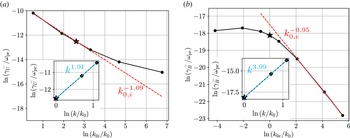


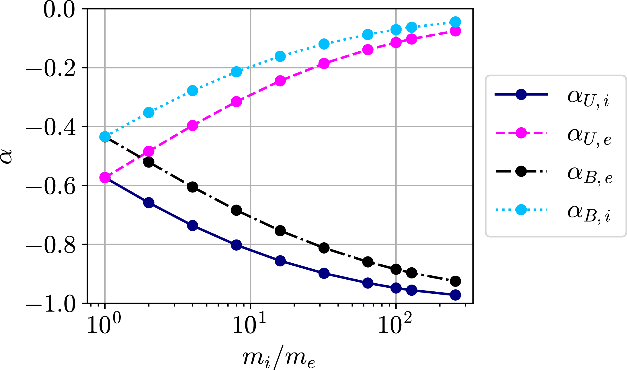


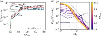


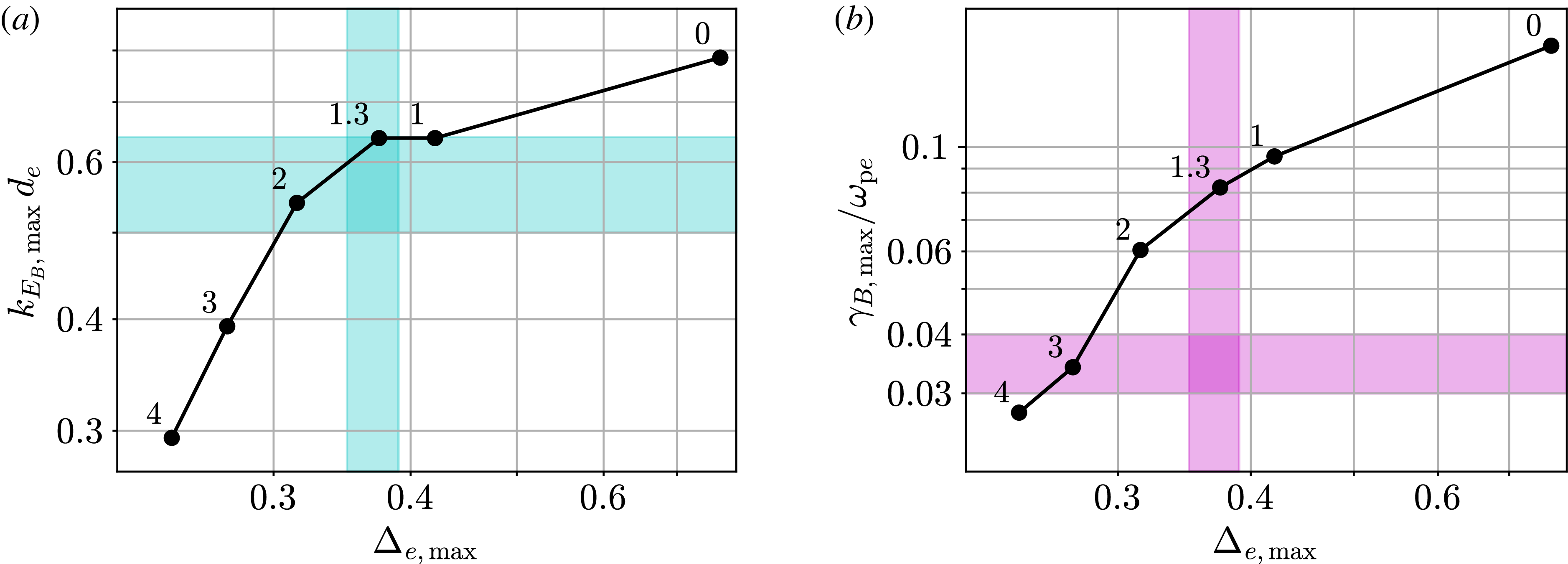


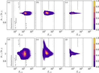


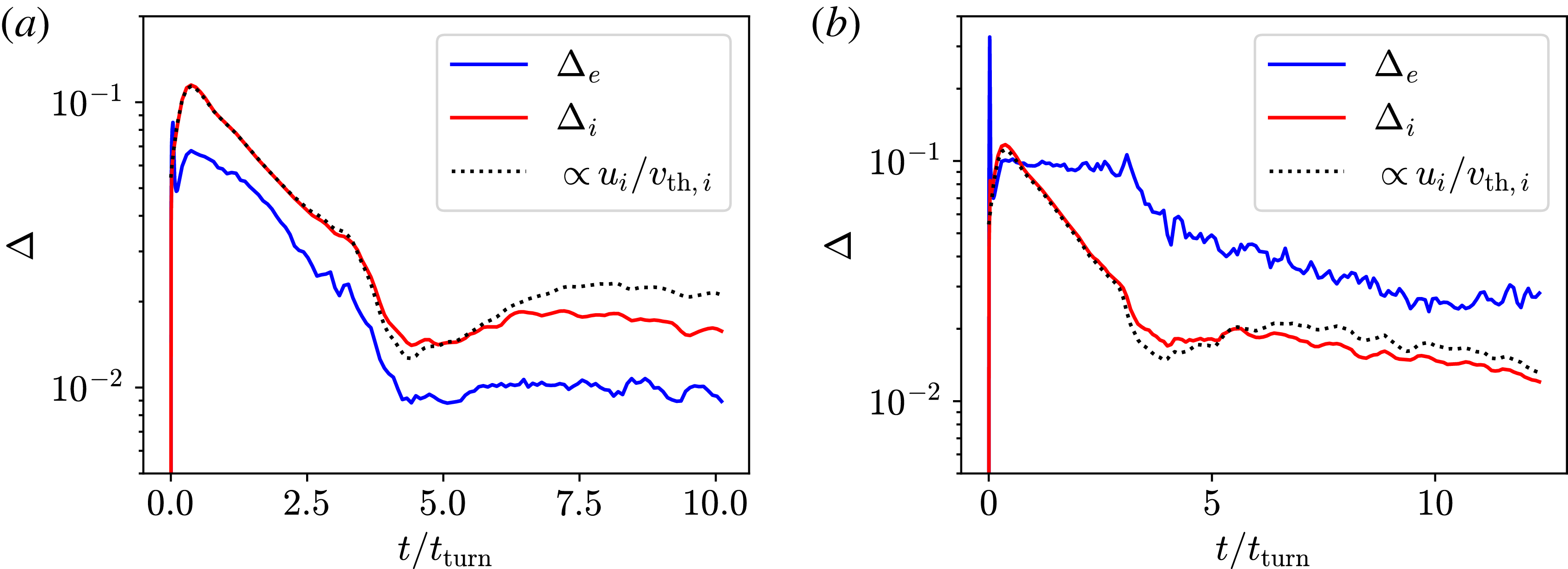


 Open access

